Mr

Ya

b

a

ARR2A

KQADIMS

1

vtso[Ipai

shbhca

t

h0

Electric Power Systems Research 144 (2017) 233–242

Contents lists available at ScienceDirect

Electric Power Systems Research

j o ur na l ho mepage: www.elsev ier .com/ locate /epsr

odeling power networks using dynamic phasors in the dq0eference frame

oash Levrona,∗, Juri Belikovb

The Andrew and Erna Viterbi Faculty of Electrical Engineering, Technion—Israel Institute of Technology, Haifa 3200003, IsraelFaculty of Mechanical Engineering, Technion—Israel Institute of Technology, Haifa 3200003, Israel

r t i c l e i n f o

rticle history:eceived 26 July 2016eceived in revised form0 November 2016ccepted 28 November 2016

eywords:uasi staticverage signalsynamic phasors

nter-area oscillationsulti-machine

tability

a b s t r a c t

The dynamic behavior of large power systems has been traditionally studied by means of time-varyingphasors, under the assumption that the system is quasi-static. However, with increasing integration of fastrenewable and distributed sources into power grids, this assumption is becoming increasingly inaccurate.In this paper, we present a dynamic model of general transmission and distribution networks that usesdynamic phasors in the dq0 reference frame. The model is formulated in the frequency domain, and isbased on the network frequency dependent admittance matrix. We also present a simplified version ofthis model that is obtained by a first-order Taylor approximation of the dynamic equations. The proposedmodels extend the quasi-static model to higher frequencies, while employing dq0 signals that are staticat steady-state, and therefore combine the advantages of high bandwidth and a well-defined operatingpoint. The models are verified numerically using the 9-, 30-, and 118-bus test-case networks. Simulationsshow that frequency responses of all models coincide at low frequencies and diverge at high frequencies.In addition, responses of the dq0 model in the time domain and in the abc reference frame are very closeto those of the transient model.

© 2016 Elsevier B.V. All rights reserved.

. Introduction

Dynamic processes occurring in large electric power systems are modeled at varying levels of abstraction [1,2]. In simple static models,oltages and currents are assumed to be sinusoidal, and are represented by phasors. The network is typically described in this case byhe power flow equations. On the other extreme, transient models describe the system using nonlinear differential equations, which areolved numerically in the time domain [3–8]. A third type of model, based on time-varying phasors, is called the average-value, dynamicr quasi-static model [2]. This model is sufficiently accurate as long as phasors are slowly changing in comparison to the system frequency9,10]. A key advantage of the quasi-static model is that it enables long numeric step times, and hence can accelerate the simulation process.n addition, since the quasi-static model employs phasors instead of sinusoidal AC signals, the system operating point is well-defined, aroperty which considerably simplifies stability studies. Due to these properties, quasi-static models have been used extensively in thenalysis of dynamic interactions that occur in time frames of seconds to minutes, and have historically enabled studies of machines stability,nter-area oscillation, and slow dynamic phenomena [1–3,11].

In recent years, with the emergence of small distributed generators and fast power electronics based devices, the assumption of quasi-tatic phasors is becoming increasingly inaccurate. Due to these emerging technologies, voltage and current signals can contain higharmonic components, and can exhibit fast amplitude and phase variations [9]. These developments have led to a new class of modelsased on dynamic phasors. The concept of dynamic phasors has emerged from averaging techniques employed in power electronics, andas been extended to three-phase systems [12]. Dynamic phasors generalize the idea of quasi-static phasors, and represent voltage andurrent signals by Fourier series expansions in which the harmonic components are evaluated over a moving time window [13]. This

pproach offers the benefits of a phasor based analysis, high accuracy, and fast simulations [14,15].

Due to these properties, dynamic phasors have been used in the analysis of synchronous and induction machines [12,16], HVDC sys-ems [14,17,18], FACTS devices [10], sub-synchronous resonance [19,20], asymmetric systems [12,21], and asymmetric faults [16,22]. For

∗ Corresponding author.E-mail addresses: yoashl@ee.technion.ac.il (Y. Levron), juri.belikov@ttu.ee (J. Belikov).

ttp://dx.doi.org/10.1016/j.epsr.2016.11.024378-7796/© 2016 Elsevier B.V. All rights reserved.

234 Y. Levron, J. Belikov / Electric Power Systems Research 144 (2017) 233–242

idtidtcesv

tdTmoetm

ts

2

w

wtqt

Udt

T

Fig. 1. A unit in the network, showing signals in the abc reference frame.

nstance, a dynamic phasor model of a line commutated HVDC converter is presented in [14]. The model represents the low-frequencyynamics of the converter, and has lower computational requirements than a conventional transient model. A dynamic phasor represen-ation of an unbalanced radial distribution system is presented in [21], where various components including a photovoltaic source and annduction machine are modeled, and dynamic interaction of these components is shown. A simulator based on dynamic phasors has beeneveloped in [15,23], which uses differential switched-algebraic state-reset equations to describe the system components. The simulationool combines advantages of transient stability and electro-magnetic simulation programs, and is demonstrated on the IEEE 39 bus test-ase network. Work [24] extends the dynamic phasor concept to multi-generator, multi-frequency systems. The theory presented in [24]nables study of electric power systems without assuming a single frequency. The proposed approach is validated on a twin-generatorystem, and can be extended to larger networks. In addition, dynamic phasors are utilized in state estimation [25–29], in systems witharying frequencies [30], and also in microgrids [31].

These recent works are mainly focused on modeling specific generators and loads, and do not provide a complete model of largeransmission networks. To bridge this gap, this paper presents a dynamic model of general transmission and distribution networks usingynamic phasors in the dq0 reference frame, and shows how this model can be implemented in practice using time-domain state equations.he first model presented in this work is formulated in the frequency domain, and is based on the network frequency dependent admittanceatrix. Since a direct numeric implementation of this model is challenging in general, we present a simplified version of it called the first-

rder dq0 model, which is obtained by a first-order Taylor approximation of the dynamic equations. The proposed frequency-domain modelxtends the quasi-static model to higher frequencies, while employing dq0 signals that are static at steady-state, and therefore combineshe advantages of high bandwidth and a well-defined operating point. The standard quasi-static model follows as a special case from the

odel at low frequencies.The paper continues as follows. Section 2 recalls basic concepts of dynamic phasors and explains how to formulate quasi-static models in

erms of dq0 quantities. Section 3 presents the proposed dq0 model. The first-order dq0 model is presented in Section 4. Section 5 providesimple illustrative examples, followed by various numerical results provided in Section 6. Concluding remarks are drawn in Section 7.

. Dynamic phasors in the dq0 reference frame

For systems in steady-state, the dq0 transformation maps sinusoidal signals to constant quantities. This transformation is compatibleith standard electric machine models, and with emerging models of renewable and distributed generators [10,15,32,33].

Assume a general power network containing N three-phase units, with voltages and currents as presented in Fig. 1.The dq0 transformation (as defined in [26]) is given by

⎡⎢⎣

xd(t)

xq(t)

x0(t)

⎤⎥⎦ = 2

3

⎡⎢⎢⎢⎢⎢⎣

cos(ωst) cos(

ωst − 2�

3

)cos

(ωst + 2�

3

)

− sin(ωst) − sin(

ωst − 2�

3

)− sin

(ωst + 2�

3

)

12

12

12

⎤⎥⎥⎥⎥⎥⎦

⎡⎢⎣

xa(t)

xb(t)

xc(t)

⎤⎥⎦ , (1)

here ωs is the nominal system frequency, and x is replaced with either a voltage (vn) or a current (in) signal. A prominent feature ofhe dq0 transformation is that for balanced and static systems, the direct and quadrature components xd, xq are constants, and x0 = 0. In auasi-static system xa, xb, xc are nearly sinusoidal, with slowly varying amplitudes and phases. In this case, the system can be modeled inerms of time-varying phasors, which are defined in terms of the dq0 components as

Vn(t) = 1√2

(vd

n(t) + jvqn(t)

), In(t) = 1√

2

(idn(t) + jiqn(t)

). (2)

nder the quasi-static approximation these dq components are identical to the xy components, as described in [34]. The following analysisefines the standard quasi-static model and power flow equations in terms of dq0 signals. Quasi-static networks are usually described byhe admittance matrix Ybus. Define the vectors:

Vd(t) =[vd

1(t), . . ., vdN(t)

]T, Id(t) =

[id1(t), . . ., idN(t)

]T, Vq(t) =

[vq

1(t), . . ., vqN(t)

]T, Iq(t) =

[iq1(t), . . ., iqN(t)

]T,

V0(t) =[v0

1(t), . . ., v0N(t)

]T, I0(t) =

[i01(t), . . ., i0N(t)

]T. (3)

hen the complex voltage and current phasors relate by

Id(t) + jIq(t) = Ybus(

Vd(t) + jVq(t))

(4)

a

T

It

et

3

vs

T

a

P

Sp

A

S

Y. Levron, J. Belikov / Electric Power Systems Research 144 (2017) 233–242 235

nd the real and imaginary parts of this equations are

Id(t) = Re{

Ybus}

Vd(t) − Im{

Ybus}

Vq(t), Iq(t) = Im{

Ybus}

Vd(t) + Re{

Ybus}

Vq(t). (5)

hese equations constitute a quasi-static model. Equivalently, quasi-static networks are also described by the power flow equations [33]

Pn(t) = |Vn(t)|N∑

k=1

|ynk||Vk(t)| cos(

∠ynk + ık − ın

), Qn(t) = −|Vn(t)|

N∑k=1

|ynk||Vk(t)| sin(

∠ynk + ık − ın

). (6)

n which the constants ynk are elements of the network admittance matrix Ybus, and powers, amplitudes and phases are formulated inerms of dq0 signals as

Pn(t) = Re{

Vn(t)In(t)∗} = 12

(vd

n(t)idn(t) + vqn(t)iqn(t)

), Qn(t) = Im

{Vn(t)In(t)∗} = 1

2

(vq

n(t)idn(t) − vdn(t)iqn(t)

),

∣∣Vn(t)∣∣ = 1√

2

√(vd

n(t))2 +

(vq

n(t))2

, ın(t) = ∠Vn(t) = atan2(vq

n(t), vdn(t)

). (7)

If the system is not quasi-static, the phasors above can be generalized by dynamic phasors. These can be defined by a Fourier seriesxpansion, as in [16]. However, to simplify notations, we have chosen in this paper to define dynamic phasors with respect to the Fourierransform as⎡

⎢⎣Vd

n (ω)

Vqn (ω)

V0n (ω)

⎤⎥⎦ =

∫ ∞

−∞

⎡⎢⎣

vdn(t)

vqn(t)

v0n(t)

⎤⎥⎦ e−jωtdt,

⎡⎢⎣

Idn(ω)

Iqn(ω)

I0n(ω)

⎤⎥⎦ =

∫ ∞

−∞

⎡⎢⎣

idn(t)

iqn(t)

i0n(t)

⎤⎥⎦ e−jωtdt. (8)

. Large network dynamics in the dq0 reference frame

The power flow equations and the equivalent dq0 model in (5), (6) are only valid under the quasi-static approximation, assuming slowariations in amplitudes and phases [34]. The following theorem extends the quasi-static model to higher frequencies, and describes theystem dynamics for general dq0 signals.

heorem 1. In symmetric power networks, a dynamic model based on dq0 dynamic phasors can be described as⎡⎢⎣

Id(ω)

Iq(ω)

I0(ω)

⎤⎥⎦ =

⎡⎣ U(ω) jR(ω) 0

−jR(ω) U(ω) 0

0 0 Ybus(ω)

⎤⎦

⎡⎢⎣

Vd(ω)

Vq(ω)

V0(ω)

⎤⎥⎦ . (9)

The following definitions are used in (9):

U(ω):=12

(Ybus(ω + ωs) + Ybus(ω − ωs)

), R(ω):=1

2

(Ybus(ω + ωs) − Ybus(ω − ωs)

), (10)

nd

Vd(ω) =[Vd

1 (ω), . . ., VdN(ω)

]T, Id(ω) =

[Id1(ω), . . ., Id

N(ω)]T

, Vq(ω) =[Vq

1 (ω), . . ., VqN(ω)

]T, Iq(ω) =

[Iq1(ω), . . ., Iq

N(ω)]T

,

V0(ω) =[V0

1 (ω), . . ., V0N(ω)

]T, I0(ω) =

[I01(ω), . . ., I0

N(ω)]T

. (11)

roof. Following the definition of the dq0 transformation in (1), voltages and currents can be expressed as sums of three elements

Va(t) = Vd(t) cos(ωst) − Vq(t) sin(ωst) + V0(t), Ia(t) = Id(t) cos(ωst) − Iq(t) sin(ωst) + I0(t). (12)

imilar expressions apply to phases b, c with a proper phase-shift of ±2�/3. Transformation to the frequency domain using the modulationroperty yields

Va(ω) = 12

(Vd(ω − ωs) + Vd(ω + ωs) + jVq(ω − ωs) − jVq(ω + ωs)

)+ V0(ω),

Ia(ω) = 12

(Id(ω − ωs) + Id(ω + ωs) + jIq(ω − ωs) − jIq(ω + ωs)

)+ I0(ω). (13)

ccording to definition[Ia1(ω) · · · Ia

N(ω)]T = Ybus(ω)

[Va

1 (ω) · · · VaN(ω)

]T. (14)

ubstituting (14) in (13) yields

Id(ω − ωs) + Id(ω + ωs) + jIq(ω − ωs) − jIq(ω + ωs) + 2I0(ω)

= Ybus(ω)(

Vd(ω − ωs) + Vd(ω + ωs) + jVq(ω − ωs) − jVq(ω + ωs) + 2V0(ω))

. (15)

2

U

w

t

C

q

4

fida

wq

Id

S

w

36 Y. Levron, J. Belikov / Electric Power Systems Research 144 (2017) 233–242

sing relation (10), equation (15) can be rewritten as

Id(ω − ωs) + Id(ω + ωs) + jIq(ω − ωs) − jIq(ω + ωs) + 2I0(ω) = 2Ybus(ω)V0(ω) + U(ω − ωs)Vd(ω − ωs) + jR(ω − ωs)Vq(ω − ωs)

+ U(ω + ωs)Vd(ω + ωs) + jR(ω + ωs)Vq(ω + ωs) + j(−jR(ω − ωs)Vd(ω − ωs) + U(ω − ωs)Vq(ω − ωs)) − j(−jR(ω + ωs)Vd(ω + ωs)

+ U(ω + ωs)Vq(ω + ωs)), (16)

hich after comparison of coefficients results in (9). �

Note that Theorem 1 holds for symmetric networks, in which the matrix Ybus(ω) equally applies to each of the three phases. However,he generators and loads connected to the network are not necessarily linear or symmetric.

The following corollary relates the proposed dq0 model to the standard quasi-static model.

orollary 1. When Ybus(ω + ωs) = Ybus and Ybus(ω − ωs) = (Ybus)∗, equation (9) reduces to the quasi-static expressions in (5).

This corollary states that if the general Ybus(ω + ωs) can be approximated by a constant matrix when ω → 0, then the dynamic model isuasi-static.

. The first-order dq0 model

Since the full dq0 model in (9) is, in general, hard to implement numerically, this section presents a simplified version of it called therst-order dq0 model, which is obtained by a first-order Taylor approximation of the dynamic equations. In this case it is assumed that theq0 signals are bandlimited, and have significant energy only at low frequencies. This enables representation of the admittance matrix by

Taylor series around ω = 0 as

Ybus(ω + ωs) ≈M∑

k=0

ωk

k!∂Ybus(ω + ωs)

∂ωk|ω=0,

Ybus(ω − ωs) ≈M∑

k=0

ωk

k!∂Ybus(ω − ωs)

∂ωk|ω=0, =

M∑k=0

(jω)k jk

k!

(∂Ybus(ω + ωs)

∂ωk

)∗|ω=0,

Ybus(ω) ≈M∑

k=0

ωk

k!∂Ybus(ω)

∂ωk|ω=0,

(17)

here in the expression for Ybus(ω − ωs) we have utilized Ybus(ω) = (Ybus(−ω))∗

and employed nested functions derivatives. The standarduasi-static approximation is obtained by a zero-order Taylor series with M = 0 such that

Ybus(ω + ωs) ≈ Ybus(ωs), Ybus(ω − ωs) ≈(

Ybus(ωs))∗

. (18)

f these expressions are substituted into the original model (9), then the model reduces to the quasi-static equations in (5). A more accurateynamic model is obtained by the first-order Taylor series approximation (M = 1) as

Ybus(ω + ωs) ≈ Ybus(ωs) + jωF, Ybus(ω − ωs) ≈ (Ybus(ωs))∗ + jωF∗, Ybus(ω) ≈ Ybus(0) + jωF0, F = −j

∂Ybus(ω + ωs)∂ω

|ω=0,

F0 = −j∂Ybus(ω)

∂ω|ω=0. (19)

ubstitution of these expressions in (9) yields

⎡⎢⎣

Id(ω)

Iq(ω)

I0(ω)

⎤⎥⎦ = (M2 + M1jω)

⎡⎢⎣

Vd(ω)

Vq(ω)

V0(ω)

⎤⎥⎦ (20)

ith

M1 =

⎡⎣ Re{F} −Im{F} 0

Im{F} Re{F} 0

0 0 F0

⎤⎦ , M2 =

⎡⎢⎣

Re{

Ybus(ωs)}

−Im{

Ybus(ωs)}

0

Im{

Ybus(ωs)}

Re{

Ybus(ωs)}

0

0 0 Ybus(0)

⎤⎥⎦ . (21)

This model can be implemented in practice using a linear state-space model

dx

dt= Ax + Bu

y = Cx + Du,

(22)

Y. Levron, J. Belikov / Electric Power Systems Research 144 (2017) 233–242 237

Fig. 2. Example 1: a network with a single inductor.

wra

C

F

Tr

I

T

5

I

N

Aa[

w

Fig. 3. Example 2: long transmission line feeding a matched load.

here u = (Vd(t), Vq(t), V0(t))T, y = (Id(t), Iq(t), I0(t))

T. The matrices A, B, C, D are chosen such that at low frequencies the frequency

esponse of the state-space model (22) is equal to (20). The general frequency response is given by y(ω) = (C(jωI − A)−1B + D)u(ω), and ispproximated at ω → 0 by

y(ω) ≈(

C(−A−1

(I + jωA−1

))B + D

)u(ω)

=(−CA−1B + D − jωCA−2B

)u(ω).

(23)

omparison of (23) and (20) provides

−CA−2B = M1, −CA−1B + D = M2. (24)

rom (24), C, D can be computed for any full-rank matrices A, B as

C = −M1B−1A2, D = M2 − M1B−1AB. (25)

he matrices A, B can be arbitrarily chosen. It is typically beneficial to select A, B such that D = 0, to obtain zero gain at ω → ∞. This criterionesults in

D = M2 − M1B−1AB ⇒ A = BM−11 M2B−1. (26)

n general, if the matrix M1 is not full-rank, then A can be computed by solving a standard least-squares minimization problem

A = BPB−1, P = arg minX

‖M1X − M2‖22. (27)

he matrix B can be arbitrarily chosen, for instance B = I.

. Dynamic dq0 models: simple examples

The simple network in Fig. 2 demonstrates the difference between the quasi-static model and the full dq0 model.In this example, the quasi-static model (5) provides

Vd(ω) = −ωsLIq(ω), Vq(ω) = ωsLId(ω). (28)

n comparison, the dq0 model can be computed by (9), and results in

Vd(ω) = jωLId(ω) − ωsLIq(ω), Vq(ω) = ωsLId(ω) + jωLIq(ω), V0(ω) = jωLI0(ω). (29)

ote that when ω → 0 the quasi-static and the dq0 models are equivalent.Another example (Fig. 3) is the long transmission line. In this example the dq0 dynamic phasors are shown to relate through time delays.

ssume a long power line of length l. The line is lossless, with inductance Lx and capacitance Cx per unit length. It feeds a matched load withn impedance equal to the characteristic impedance Zc =

√Lx/Cx. The resulting load current is delayed in respect to the source voltage

33] as

iabc2 (t) = 1

Zcvabc

1 (t − d), (30)

here the time delay is given by d = l√

LxCx.

238 Y. Levron, J. Belikov / Electric Power Systems Research 144 (2017) 233–242

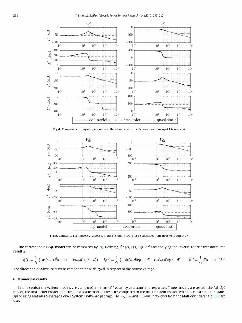
Fig. 4. Comparison of frequency responses in the 9-bus network for dq quantities from input 1 to output 4.

r

T

6

msu

Fig. 5. Comparison of frequency responses in the 118-bus network for dq quantities from input 76 to output 77.

The corresponding dq0 model can be computed by (9). Defining Ybus(ω) = (1/Zc)e−jωd and applying the inverse Fourier transform, theesult is

id2(t) = 1Zc

(cos(ωsd)vd

1(t − d) + sin(ωsd)vq1(t − d)

), iq2(t) = 1

Zc

(− sin(ωsd)vd

1(t − d) + cos(ωsd)vq1(t − d)

), i02(t) = 1

Zcv0

1(t − d). (31)

he direct and quadrature current components are delayed in respect to the source voltage.

. Numerical results

In this section the various models are compared in terms of frequency and transient responses. Three models are tested: the full dq0

odel, the first-order model, and the quasi-static model. These are compared to the full transient model, which is constructed in state-

pace using Matlab’s Simscape Power Systems software package. The 9-, 30-, and 118-bus networks from the MatPower database [35] aresed.

Y. Levron, J. Belikov / Electric Power Systems Research 144 (2017) 233–242 239

Fig. 6. Comparison of the first 100 largest Hankel singular values of the dq0 model and the first-order model in the 118-bus network.

1ticafe

tfi

pmm(

at

prhsc

Fig. 7. Comparison of step-responses in the 9-bus system. The inputs (bottom plot) are steps in phases a, b, c at bus 1. The output is the current of phase a at bus 4.

An array of Bode plots representing the dq0, first-order, and quasi-static models is graphically illustrated in Figs. 4 and 5 for 9- and18-bus networks. The plots depict the magnitude (in dB) and phase (in degrees) for several input/output pairs. The step input is appliedo a generator located at bus 1 and the output is measured at bus 4 for the case of 9-bus network. Similarly, for 118-bus network the stepnput is applied to a generator located at bus 76 and the output is measured at bus 77. The figures show that the frequency responsesoincide at low frequencies (ω → 0) and diverge at high frequencies. Specifically, the quasi-static model is represented by a constant gain,nd has a constant gain and phase at all frequencies. The first-order model response coincides with the dq0 model response over a widerrequency range and deviates only at high frequencies. These figures illustrate the main result presented in Theorem 1 that dq0 modelxtends both quasi-static and first-order models by taking high-frequency dynamic phenomena into account.

Fig. 6 compares the largest singular values of the dq0 model and the first-order model for the 118-bus network. It can be seen thathe most energetic (largest) values are similar, meaning that the majority of energy is preserved. This in turn verifies the quality of therst-order model.

Figs. 7–11 compare the transient response of the various models for the 9-, 30- and 118-bus networks. All inputs and outputs are threehase signals. The transient model is simulated directly in the abc reference frame. The dq0 model, quasi-static model, and the first-orderodel are represented in the dq0 reference frame, so input and output signals are converted accordingly using (1). To this end, the dq0odel is represented in the state-space form using implementation available in [36]. The first-order model is implemented using equations

22)–(27).Figs. 7 and 8 provide simulation results for the case of 9-bus network. In Fig. 7 the step input signals (shifted in time for each of the phases)

re applied to the generator 1 at bus 1 and the outputs are measured at bus 4. In Fig. 8 a more complicated scenario is considered. Beforehe transient, the inputs are balanced three phase sinusoidal signals ua

1 = sin(2�50t) at bus 1. Then, the transient is triggered by shorting

hase a to ground, i.e., ua1 = 0. Note that uc,d

1 = sin(2�50t ± 2�/3). The output is the current of phase a measured at bus 4. The simulationesults confirm the above frequency domain analysis presented in Fig. 4 and the fact that the quasi-static model becomes inaccurate atigh frequencies. The similar settings were used to obtain simulation results for the 30- and 118-bus networks (see Figs. 9–11). The figures

how that transient responses of the dq0 models are similar to those of the transient models. The quasi-static model is implemented byonstant gains, and is inaccurate, except for balanced sinusoidal inputs. The first-order model is moderately accurate.

240 Y. Levron, J. Belikov / Electric Power Systems Research 144 (2017) 233–242

Fig. 8. Comparison of transients in the 9-bus system. Before the transient, the inputs are balanced three phase sinusoidal signals at bus 1. The transient is triggered byshorting phase a to ground. The output is the current of phase a at bus 4.

Fig. 9. Comparison of step responses in the 30-bus network. The inputs are steps at t = 0 in phases a, b, c. (a) input at bus 1, output at bus 2, (b) input at bus 5, output at bus7, (c) input at bus 8, output at bus 28, (d) input at bus 11, output at bus 9.

Table 1Errors in transient responses.

Fig. 7 Fig. 8(a) Fig. 10 Fig. 11(a)

MSEdq0 0.9595 × 10−8 0.9572 × 10−9 0.6557 × 10−8 0.9340 × 10−7

fo 0.0035 3.4425 × 10−5 4.6116 × 10−5 4.9407 × 10−4

qs 0.1929 0.0020 0.0039 0.0170

ISEdq0 0.7922 × 10−8 0.9706 × 10−9 0.3570 × 10−8 0.8491 × 10−7

fo 0.0035 3.4446 × 10−5 1.1498 × 10−5 1.2363 × 10−4

qs 0.1913 0.0020 9.6554 × 10−4 0.0042

Y. Levron, J. Belikov / Electric Power Systems Research 144 (2017) 233–242 241

Fig. 10. Comparison of step-responses in the 118-bus system. The inputs (bottom plot) are steps in phases a, b, c of bus 76. The output is the current of phase a at bus 77.

Fs

is

7

tgdamid

ig. 11. Comparison of transients in the 118-bus system. Before the transient, the inputs are balanced three phase sinusoidal signals at bus 76. The transient is triggered byhorting phase a to ground. The output is the current of phase a at bus 77.

Errors in the models transient responses are presented in Table 1, where two typical metrics, the mean squared error (MSE) and thentegral squared error (ISE), are used. The errors are calculated in comparison to the transient model, which serves as a reference. It can beeen that the magnitudes of errors for the dq0 model are significantly lower than those of first-order and quasi-static models.

. Conclusion

Dynamic behavior and stability of large-scale power systems have been traditionally studied by means of time-varying phasors, underhe assumption that the system is quasi-static. However, with increasing integration of fast renewable and distributed sources into powerrids, this assumption is becoming increasingly inaccurate. This paper uses dynamic phasors in the dq0 reference frame to describe theynamics of large transmission and distribution networks. The proposed models do not employ the assumption of quasi-static phasors,

nd therefore remain accurate over a wide range of frequencies. The full dq0 model is based on the frequency dependent admittanceatrix, and is approximated using the Taylor series expansion to generate models of lower complexity: the classic quasi-static model

s obtained by a zero-order approximation, while the more accurate first-order model is obtained by a first-order approximation. Theeveloped models combine two properties of interest. On one hand, they provide the advantages of the dq0 reference frame. Specifically,

2

thpcma

A

R

[[

[

[[

[

[[[

[

[

[[

[[

[

[

[

[

[[

[

[[[[

[

42 Y. Levron, J. Belikov / Electric Power Systems Research 144 (2017) 233–242

he models employ nonrotating dq0 signals that are static at steady-state, and thus enable a well-defined operating point. On the otherand, the proposed models improve the accuracy of the quasi-static model at high frequencies, enabling representation of fast dynamichenomena in networks that include small distributed generators and fast power electronics based devices. In particular, these propertiesan contribute to accurate and low complexity stability analysis in such networks. Simulations show that the frequency responses of allodels coincide at low frequencies and diverge at high frequencies. In addition, responses of the dq0 model in the time domain and in the

bc reference frame are very close to those of the transient model.

cknowledgment

The work was partly supported by Grand Technion Energy Program (GTEP) and a Technion fellowship.

eferences

[1] Y. Liu, K. Sun, Y. Liu, A measurement-based power system model for dynamic response estimation and instability warning, Electr. Power Syst. Res. 124 (2015) 1–9.[2] L. Miller, L. Cibulka, M. Brown, A.V. Meier, Electric distribution system models for renewable integration: Status and research gaps analysis, Tech. rep., California

Energy Commission, CA, USA, 2013.[3] P.M. Anderson, A.A. Fouad, Power System Control and Stability, John Wiley & Sons, 2008.[4] C. Dufour, J. Mahseredjian, J. Bélanger, A combined state-space nodal method for the simulation of power system transients, IEEE Trans. Power Del. 26 (2) (2011)

928–935.[5] U.N. Gnanarathna, A.M. Gole, R.P. Jayasinghe, Efficient modeling of modular multilevel HVDC converters (MMC) on electromagnetic transient simulation programs,

IEEE Trans. Power Del. 26 (1) (2011) 316–324.[6] R. Majumder, Some aspects of stability in microgrids, IEEE Trans. Power Syst. 28 (3) (2013) 3243–3252.[7] T. Nishikawa, A.E. Motter, Comparative analysis of existing models for power-grid synchronization, New J. Phys. 17 (1) (2015).[8] R. Zárate-Mi nano, T.V. Cutsem, F. Milano, J.A. Conejo, Securing transient stability using time-domain simulations within an optimal power flow, IEEE Trans. Power

Syst. 25 (1) (2010) 243–253.[9] M. Ilic, J. Zaborszky, Quasistationary phasor concepts, in: Dynamics and Control of Large Electric Power Systems, Wiley, New York, 2000, pp. 9–60.10] P.C. Stefanov, A.M. Stankovic, Modeling of UPFC operation under unbalanced conditions with dynamic phasors, IEEE Trans. Power Syst. 17 (2) (2002) 395–403.11] R. Yousefian, S. Kamalasadan, A Lyapunov function based optimal hybrid power system controller for improved transient stability, Electr. Power Syst. Res. 137 (2016)

6–15.12] A.M. Stankovic, S.R. Sanders, T. Aydin, Dynamic phasors in modeling and analysis of unbalanced polyphase A machines, IEEE Trans. Energy Convers. 17 (1) (2002)

107–113.13] S. Almer, U. Jonsson, Dynamic phasor analysis of periodic systems, IEEE Trans. Autom. Control 54 (8) (2009) 2007–2012.14] M. Daryabak, S. Filizadeh, J. Jatskevich, A. Davoudi, M. Saeedifard, V.K. Sood, J.A. Martinez, D. Aliprantis, J. Cano, A. Mehrizi-Sani, Modeling of LCC-HVDC systems using

dynamic phasors, IEEE Trans. Power Del. 29 (4) (2014) 1989–1998.15] T. Demiray, G. Andersson, L. Busarello, Evaluation study for the simulation of power system transients using dynamic phasor models, in: Transmission and Distribution

Conf. and Expo, Bogotá, Colombia, 2008, pp. 1–6.16] A.M. Stankovic, T. Aydin, Analysis of asymmetrical faults in power systems using dynamic phasors, IEEE Trans. Power Syst. 15 (3) (2000) 1062–1068.17] C. Liu, A. Bose, P. Tian, Modeling and analysis of HVDC converter by three-phase dynamic phasor, IEEE Trans. Power Del. 29 (1) (2014) 3–12.18] H. Zhu, Z. Cai, H. Liu, Q. Qi, Y. Ni, Hybrid-model transient stability simulation using dynamic phasors based HVDC system model, Electr. Power Syst. Res. 76 (6-7) (2006)

582–591.19] M.C. Chudasama, A.M. Kulkarni, Dynamic phasor analysis of SSR mitigation schemes based on passive phase imbalance, IEEE Trans. Power Syst. 26 (3) (2011)

1668–1676.20] P. Mattavelli, A.M. Stankovic, G.C. Verghese, SSR analysis with dynamic phasor model of thyristor-controlled series capacitor, IEEE Trans. Power Syst. 14 (1) (1999)

200–208.21] Z. Miao, L. Piyasinghe, J. Khazaei, L. Fan, Dynamic phasor-based modeling of unbalanced radial distribution systems, IEEE Trans. Power Syst. 30 (6) (2015) 3102–3109.22] S. Chandrasekar, R. Gokaraju, Dynamic phasor modeling of type 3 DFIG wind generators (including SSCI phenomenon) for short-circuit calculations, IEEE Trans. Power

Del. 30 (2) (2015) 887–897.23] T.H. Demiray, Simulation of power system dynamics using dynamic phasor models. Ph.D. thesis, TU Wien, 2008.24] T. Yang, S. Bozhko, G. Asher, Multi-generator system modelling based on dynamic phasor concept, in: European Conf. on Power Electronics and Applications, Lille,

France, 2013, pp. 1–10.25] T. Bi, H. Liu, Q. Feng, C. Qian, Y. Liu, Dynamic phasor model-based synchrophasor estimation algorithm for M-class PMU, IEEE Trans. Power Del. 30 (3) (2015)

1162–1171.26] D.-G. Lee, S.-H. Kang, S.-R. Nam, Modified dynamic phasor estimation algorithm for the transient signals of distributed generators, IEEE Trans. Smart Grids 4 (1) (2013)

419–424.27] R.K. Mai, L. Fu, Z.Y. Dong, K.P. Wong, Z.Q. Bo, H.B. Xu, Dynamic phasor and frequency estimators considering decaying DC components, IEEE Trans. Power Syst. 27 (2)

(2012) 671–681.28] R.K. Mai, L. Fu, Z.Y. Dong, B. Kirby, Z.Q. Bo, An adaptive dynamic phasor estimator considering DC offset for PMU applications, IEEE Trans. Power Del. 26 (3) (2011)

1744–1754.29] J. Ren, M. Kezunovic, An adaptive phasor estimator for power system waveforms containing transients, IEEE Trans. Power Del. 27 (2) (2012) 735–745.30] T. Yang, S. Bozhko, J.M. Le-Peuvedic, G. Asher, C.I. Hill, Dynamic phasor modeling of multi-generator variable frequency electrical power systems, IEEE Trans. Power

Syst. 31 (1) (2016) 563–571.31] X. Guo, Z. Lu, B. Wang, X. Sun, L. Wang, J.M. Guerrero, Dynamic phasors-based modeling and stability analysis of droop-controlled inverters for microgrid applications,

IEEE Trans. Smart Grids 5 (6) (2014) 2980–2987.32] A.E. Fitzgerald, C. Kingsley, S.D. Umans, Electric Machinery, 6th ed., McGraw-Hill, New York, 2003.33] J.J. Grainger, W.D. Stevenson, Power System Analysis, McGraw-Hill, New York, 1994.

34] T.V. Cutsem, C. Vournas, Voltage Stability of Electric Power Systems, Kluwer Academic Publishers, Norwell, MA, 1998.35] R.D. Zimmerman, C.E. Murillo-Sánchez, R.J. Thomas, MATPOWER: steady-state operations planning and analysis tools for power systems research and education, IEEE

Trans. Power Syst. 26 (1) (2011) 12–19.36] Y. Levron, J. Belikov, Toolbox for modeling and analysis of power networks in the dq0 reference frame, MATLAB Central File Exchange, 2016 http://www.mathworks.

com/matlabcentral/fileexchange/58702 (retrieved 15.08.16).