TAIL RISK RESEARCH PROGRAM

Election Predictions as Martingales: An ArbitrageApproach

Nassim Nicholas TalebTandon School of Engineering, New York University 3rd Version, October 2017

Forthcoming, Quantitative Finance

I. INTRODUCTION

A standard result in quantitative finance is that when thevolatility of the underlying security increases, arbitrage pres-sures push the corresponding binary option to trade closerto 50%, and become less variable over the remaining timeto expiration. Counterintuitively, the higher the uncertainty ofthe underlying security, the lower the volatility of the binaryoption. This effect should hold in all domains where a binaryprice is produced – yet we observe severe violations of theseprinciples in many areas where binary forecasts are made, inparticular those concerning the U.S. presidential election of2016. We observe stark errors among political scientists andforecasters, for instance with 1) assessors giving the candidateD. Trump between 0.1% and 3% chances of success , 2) jumpsin the revisions of forecasts from 48% to 15%, both madewhile invoking uncertainty.

Conventionally, the quality of election forecasting has beenassessed statically by De Finetti’s method, which consistsin minimizing the Brier score, a metric of divergence fromthe final outcome (the standard for tracking the accuracyof probability assessors across domains, from elections toweather). No intertemporal evaluations of changes in estimatesappear to have been imposed outside the quantitative financepractice and literature. Yet De Finetti’s own principle is thata probability should be treated like a two-way "choice" price,which is thus violated by conventional practice.

0.42

0.44

0.46

0.48

0.5

0.04 0.06 0.08 0.10 0.12s

0.2

0.3

0.4

0.5

Estimator

Fig. 1. Election arbitrage "estimation" (i.e., valuation) at different expectedproportional votes Y ∈ [0, 1], with s the expected volatility of Y betweenpresent and election results. We can see that under higher uncertainty, theestimation of the result gets closer to 0.5, and becomes insensitive to estimatedelectoral margin.

Bt0 ∈ [0,1]

Y ∈ [L,H]

X ∈ (-∞,∞)

B= ℙ(XT > l)

B= ℙ(YT > S(l))

Y=S(X)

Fig. 2. X is an open non observable random variable (a shadow variable ofsorts) on R, Y , its mapping into "votes" or "electoral votes" via a sigmoidalfunction S(.), which maps one-to-one, and the binary as the expected valueof either using the proper corresponding distribution.

In this paper we take a dynamic, continuous-time approachbased on the principles of quantitative finance and argue thata probabilistic estimate of an election outcome by a given"assessor" needs be treated like a tradable price, that is,as a binary option value subjected to arbitrage boundaries(particularly since binary options are actually used in bettingmarkets). Future revised estimates need to be compatiblewith martingale pricing, otherwise intertemporal arbitrage iscreated, by "buying" and "selling" from the assessor.

A mathematical complication arises as we move to continu-ous time and apply the standard martingale approach: namelythat as a probability forecast, the underlying security livesin [0, 1]. Our approach is to create a dual (or "shadow")martingale process Y , in an interval [L,H] from an arith-metic Brownian motion, X in (−∞,∞) and price electionsaccordingly. The dual process Y can for example representthe numerical votes needed for success. A complication isthat, because of the transformation from X to Y , if Y is amartingale, X cannot be a martingale (and vice-versa).

The process for Y allows us to build an arbitrage relation-ship between the volatility of a probability estimate and thatof the underlying variable, e.g. the vote number. Thus we areable to show that when there is a high uncertainty about thefinal outcome, 1) indeed, the arbitrage value of the forecast(as a binary option) gets closer to 50% and 2) the estimateshould not undergo large changes even if polls or other bases

N. N. Taleb 1

arX

iv:1

703.

0635

1v3

[q-

fin.

PR]

15

Nov

201

7

TAIL RISK RESEARCH PROGRAM

show significant variations.1

The pricing links are between 1) the binary option value(that is, the forecast probability), 2) the estimation of Y and3) the volatility of the estimation of Y over the remaining timeto expiration (see Figures 1 and 2 ).

A. Main results

For convenience, we start with our notation.Notation:Y0 the observed estimated proportion of votes ex-

pressed in [0, 1] at time t0. These can be eitherpopular or electoral votes, so long as one treatsthem with consistency.

T period when the irrevocable final election out-come YT is revealed, or expiration.

t0 present evaluation period, hence T−t0 is the timeuntil the final election, expressed in years.

s annualized volatility of Y , or uncertainty attend-ing outcomes for Y in the remaining time untilexpiration. We assume s is constant without anyloss of generality –but it could be time dependent.

B(.) "forecast probability", or estimated continuous-time arbitrage evaluation of the election results,establishing arbitrage bounds between B(.), Y0and the volatility s.

Main results:

B(Y0, σ, t0, T ) =1

2erfc

(l − erf−1(2Y0 − 1)eσ

2(T−t0)√e2σ2(T−t0) − 1

),

(1)where

σ ≈

√log(2πs2e2erf−1(2Y0−1)2 + 1

)√

2√T − t0

, (2)

l is the threshold needed (defaults to .5), and erfc(.) is thestandard complementary error function, 1-erf(.), with erf(z) =2√π

∫ z0e−t

2

dt.We find it appropriate here to answer the usual comment

by statisticians and people operating outside of mathematicalfinance: "why not simply use a Beta-style distribution forY ?". The answer is that 1) the main purpose of the paper isestablishing (arbitrage-free) time consistency in binary fore-casts, and 2) we are not aware of a continuous time stochasticprocess that accommodates a beta distribution or a similarlybounded conventional one.

B. Organization

The remaining parts of the paper are organized as follows.First, we show the process for Y and the needed transfor-mations from a specific Brownian motion. Second, we derive

1A central property of our model is that it prevents B(.) from varying morethan the estimated Y : in a two candidate contest, it will be capped (floored)at Y if lower (higher) than .5. In practice, we can observe probabilities ofwinning of 98% vs. 02% from a narrower spread of estimated votes of 47%vs. 53%; our approach prevents, under high uncertainty, the probabilities fromdiverging away from the estimated votes. But it remains conservative enoughto not give a higher proportion.

the arbitrage relationship used to obtain equation (1). Finally,we discuss De Finetti’s approach and show how a martingalevaluation relates to minimizing the conventional standard inthe forecasting industry, namely the Brier Score.

A comment on absence of closed form solutions for σ: Wenote that for Y we lack a closed form solution for the integralreflecting the total variation:

∫ Tt0

σ√πe−erf−1(2ys−1)2ds, though

the corresponding one for X is computable. Accordingly, wehave relied on propagation of uncertainty methods to obtain aclosed form solution for the probability density of Y , thoughnot explicitly its moments as the logistic normal integral doesnot lend itself to simple expansions [1].

Time slice distributions for X and Y : The time slicedistribution is the probability density function of Y fromtime t, that is the one-period representation, starting at twith y0 = 1

2 + 12erf(x0). Inversely, for X given y0, the

corresponding x0, X may be found to be normally distributedfor the period T − t0 with

E(X,T ) = X0eσ2(T−t0),

V(X,T ) =e2σ

2(T−t0) − 1

2

and a kurtosis of 3. By probability transformation we obtainϕ, the corresponding distribution of Y with initial value y0 isgiven by

(3)

ϕ(y; y0, T ) =1√

e2σ2(t−t0) − 1exp

{erf−1(2y − 1)2

− 1

2

(coth

(σ2t)− 1) (

erf−1(2y − 1)

− erf−1(2y0 − 1)eσ2(t−t0)

)2}and we have E(Yt) = Y0.

As to the variance, E(Y 2), as mentioned above, does notlend itself to a closed-form solution derived from ϕ(.), norfrom the stochastic integral; but it can be easily estimatedfrom the closed form distribution of X using methods ofpropagation of uncertainty for the first two moments (the deltamethod).

Since the variance of a function f of a finite momentrandom variable X can be approximated as V (f(X)) =f ′ (E(X))

2V (X):

∂S−1(y)

∂y

∣∣∣∣y=Y0

s2 ≈ e2σ2(T−t0) − 1

2

s ≈

√e−2erf−1(2Y0−1)2

(e2σ2(T−t0) − 1

)2π

. (4)

Likewise for calculations in the opposite direction, we find

σ ≈

√log(2πs2e2erf−1(2Y0−1)2 + 1

)√

2√T − t0

,

which is (2) in the presentation of the main result.Note that expansions including higher moments do not

bring a material increase in precision – although s is highly

N. N. Taleb 2

TAIL RISK RESEARCH PROGRAM

ELECTION

DAY

538

Rigorous

updating

20 40 60 80 100

0.5

0.6

0.7

0.8

0.9

1.0

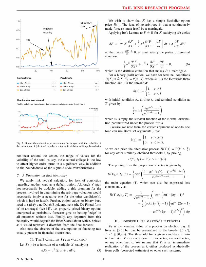
Fig. 3. Shows the estimation process cannot be in sync with the volatility ofthe estimation of (electoral or other) votes as it violates arbitrage boundaries

nonlinear around the center, the range of values for thevolatility of the total or, say, the electoral college is too lowto affect higher order terms in a significant way, in additionto the boundedness of the sigmoid-style transformations.

C. A Discussion on Risk NeutralityWe apply risk neutral valuation, for lack of conviction

regarding another way, as a default option. Although Y maynot necessarily be tradable, adding a risk premium for theprocess involved in determining the arbitrage valuation wouldnecessarily imply a negative one for the other candidate(s),which is hard to justify. Further, option values or binary bets,need to satisfy a no Dutch Book argument (the De Finetti formof no-arbitrage) (see [4]), i.e. properly priced binary optionsinterpreted as probability forecasts give no betting "edge" inall outcomes without loss. Finally, any departure from riskneutrality would degrade the Brier Score (about which, below)as it would represent a diversion from the final forecast.

Also note the absence of the assumptions of financing rateusually present in financial discussions.

II. THE BACHELIER-STYLE VALUATION

Let F (.) be a function of a variable X satisfying

dXt = σ2Xtdt+ σ dWt. (5)

We wish to show that X has a simple Bachelier optionprice B(.). The idea of no arbitrage is that a continuouslymade forecast must itself be a martingale.

Applying Itô’s Lemma to F , B for X satisfying (5) yields

dF =

[σ2X

∂F

∂X+

1

2σ2 ∂

2F

∂X2+∂F

∂t

]dt+ σ

∂F

∂XdW

so that, since ∂F∂t , 0, F must satisfy the partial differential

equation

1

2σ2 ∂

2F

∂X2+ σ2X

∂F

∂X+∂F

∂t= 0, (6)

which is the driftless condition that makes B a martingale.For a binary (call) option, we have for terminal conditions

B(X, t) , F, FT = θ(x− l), where θ(.) is the Heaviside thetafunction and l is the threshold:

θ(x) :=

{1, x ≥ l0, x < l

with initial condition x0 at time t0 and terminal condition atT given by:

1

2erfc

(x0e

σ2t − l√e2σ2t − 1

)which is, simply, the survival function of the Normal distribu-tion parametrized under the process for X .

Likewise we note from the earlier argument of one-to one(one can use Borel set arguments ) that

θ(y) :=

{1, y ≥ S(l)

0, y < S(l),

so we can price the alternative process B(Y, t) = P(Y > 12 )

(or any other similarly obtained threshold l, by pricing

B(Y0, t0) = P(x > S−1(l)).

The pricing from the proportion of votes is given by:

B(Y0, σ, t0, T ) =1

2erfc

(l − erf−1(2Y0 − 1)eσ

2(T−t0)√e2σ2(T−t0) − 1

),

the main equation (1), which can also be expressed lessconveniently as

B(Y, σ, t0, T ) =1√

e2σ2t − 1

∫ 1

l

exp

(erf−1(2y − 1)2

− 1

2

(coth

(σ2t)− 1) (

erf−1(2y − 1)

− erf−1(2y0 − 1)eσ2t)2)

dy

III. BOUNDED DUAL MARTINGALE PROCESS

YT is the terminal value of a process on election day. Itlives in [0, 1] but can be generalized to the broader [L,H],L,H ∈ [0,∞). The threshold for a given candidate to winis fixed at l. Y can correspond to raw votes, electoral votes,or any other metric. We assume that Yt is an intermediaterealization of the process at t, either produced syntheticallyfrom polls (corrected estimates) or other such systems.

N. N. Taleb 3

TAIL RISK RESEARCH PROGRAM

X

Y

200 400 600 800 1000t

-1.5

-1.0

-0.5

0.5

X,Y

Fig. 4. Process and Dual Process

Next, we create, for an unbounded arithmetic stochasticprocess, a bounded "dual" stochastic process using a sigmoidaltransformation. It can be helpful to map processes such as abounded electoral process to a Brownian motion, or to map abounded payoff to an unbounded one, see Figure 2.

Proposition 1. Under sigmoidal style transformations S :x 7→ y,R→ [0, 1] of the form a) 1

2 + 12erf(x), or b) 1

1+exp(−x) ,if X is a martingale, Y is only a martingale for Y0 = 1

2 , andif Y is a martingale, X is only a martingale for X0 = 0 .

Proof. The proof is sketched as follows. From Itô’s lemma, thedrift term for dXt becomes 1) σ2X(t), or 2) 1

2σ2Tanh

(X(t)2

),

where σ denotes the volatility, respectively with transforma-tions of the forms a) of Xt and b) of Xt under a martingale for

Y . The drift for dYt becomes: 1) σ2e−erf−1(2Y −1)2erf−1(2Y−1)√

π

or 2) 12σ

2Y (Y − 1)(2Y − 1) under a martingale for X .

We therefore select the case of Y being a martingale andpresent the details of the transformation a). The properties ofthe process have been developed by Carr [2]. Let X be thearithmetic Brownian motion (5), with X-dependent drift andconstant scale σ:

dXt = σ2Xtdt+ σdWt, 0 < t < T < +∞.

We note that this has similarities with the Ornstein-Uhlenbeck process normally written dXt = θ(µ − Xt)dt +σdW , except that we have µ = 0 and violate the rules by usinga negative mean reversion coefficient, rather more adequatelydescribed as "mean repelling", θ = −σ2.

We map from X ∈ (−∞,∞) to its dual process Y asfollows. With S : R→ [0, 1], Y = S(x),

S(x) =1

2+

1

2erf(x)

the dual process (by unique transformation since S is one toone, becomes, for y , S(x), using Ito’s lemma (since S(.) istwice differentiable and ∂S/∂t = 0):

dS =

(1

2σ2 ∂

2S

∂x2+Xσ2 ∂S

∂x

)dt+ σ

∂S

∂xdW

which with zero drift can be written as a process

dYt = s(Y )dWt,

for all t > τ,E(Yt|Yτ ) = Yτ . and scale

s(Y ) =σ√πe−erf−1(2y−1)2

which as we can see in Figure 5, s(y) can be approximatedby the quadratic function y(1− y) times a constant.

ⅇ-erf-1 (-1+2 y)2

π8π2

3

y (1 - y)

0.2 0.4 0.6 0.8 1.0Yt

0.05

0.10

0.15

0.20

0.25

s

Fig. 5. The instantaneous volatility of Y as a function of the level of Yfor two different methods of transformations of X , which appear to not besubstantially different. We compare to the quadratic form y − y2 scaledby a constant 1

3

√8π

2

. The volatility declines as we move away from 12

and collapses at the edges, thus maintaining Y in (0, 1). For simplicity weassumed σ = t = 1.

We can recover equation (5) by inverting, namely S−1(y) =erf−1(2y − 1), and again applying Itô’s Lemma. As a conse-quence of gauge invariance option prices are identical whetherpriced on X or Y , even if one process has a drift whilethe other is a martingale. In other words, one may applyone’s estimation to the electoral threshold, or to the morecomplicated X with the same results. And, to summarize ourmethod, pricing an option on X is familiar, as it is exactly aBachelier-style option price.

IV. RELATION TO DE FINETTI’S PROBABILITY ASSESSOR

This section provides a brief background for the con-ventional approach to probability assessment. De Finetti [3]has shown that the "assessment" of the "probability" of therealization of a random variable in {0, 1} requires a nonlinearloss function – which makes his definition of probabilisticassessment differ from that of the P/L of a trader engaging inbinary bets.

Assume that a betting agent in an n-repeated two periodmodel, t0 and t1, produces a strategy S of bets b0,i ∈ [0, 1]indexed by i = 1, 2, . . . , n, with the realization of the binaryr.v. 1t1,i. If we take the absolute variation of his P/L over nbets, it will be

L1(S) =1

n

n∑i=1

|1t1,i − bt0,i| .

For example, assume that E(1t1) = 12 . Betting on the

probability, here 12 , produces a loss of 1

2 in expectation, whichis the same as betting either 0 or 1 – hence not favoring theagent to bet on the exact probability.

If we work with the same random variable and non-time-varying probabilities, the L1 metric would be appropriate:

N. N. Taleb 4

TAIL RISK RESEARCH PROGRAM

L1(S) =1

n

∣∣∣∣∣1t1,i −n∑i=1

bt0,i

∣∣∣∣∣ .De Finetti proposed a "Brier score" type function, a

quadratic loss function in L2:

L2(S) =1

n

n∑i=1

(1t1,i − bt0,i)2,

the minimum of which is reached for bt0,i = E(1t1).In our world of continuous time derivative valuation, where,

in place of a two period lattice model, we are interested, for thesame final outcome at t1, in the stochastic process bt, t0 ≥ t ≥t1, the arbitrage "value" of a bet on a binary outcome needs tomatch the expectation, hence, again, we map to the Brier score– by an arbitrage argument. Although there is no quadraticloss function involved, the fact that the bet is a function ofa martingale, which is required to be itself a martingale, i.e.that the conditional expectation remains invariant to time, doesnot allow an arbitrage to take place. A "high" price can be"shorted" by the arbitrageur, a "low" price can be "bought",and so on repeatedly. The consistency between bets at period tand other periods t+ ∆t enforces the probabilistic discipline.In other words, someone can "buy" from the forecaster then"sell" back to him, generating a positive expected "return" ifthe forecaster is out of line with martingale valuation.

As to the current practice by forecasters, although someelection forecasters appear to be aware of the need to minimizetheir Brier Score, the idea that the revisions of estimatesshould also be subjected to martingale valuation is not wellestablished.

V. CONCLUSION AND COMMENTS

As can be seen in Figure 1, a binary option reveals moreabout uncertainty than about the true estimation, a result wellknown to traders, see [5].

In the presence of more than 2 candidates, the process canbe generalized with the following heuristic approximation.Establish the stochastic process for Y1,t, and just as Y1,t isa process in [0, 1], Y2,t is a process ∈ (Y1,t, 1], with Y3,t theresidual 1−Y2,t−Y1,t, and more generally Yn−1,t ∈ (Yn2,t, 1]and Yn,t is the residual Yn = 1−

∑n−1i=1 Yi,t. For n candidates,

the nth is the residual.

VI. ACKNOWLEDGEMENTS

The author thanks Dhruv Madeka and Raphael Douady fordetailed and extensive discussions of the paper as well asthorough auditing of the proofs across the various iterations,and, worse, the numerous changes of notation. Peter Carrhelped with discussions on the properties of a bounded martin-gale and the transformations. I thank David Shimko,AndrewLesniewski, and Andrew Papanicolaou for comments. I thankArthur Breitman for guidance with the literature for numeri-cal approximations of the various logistic-normal integrals. Ithank participants of the Tandon School of Engineering andBloomberg Quantitative Finance Seminars. I also thank BrunoDupire,MikeLawler, theEditors-In-Chief, and various friendly

people on social media. DhruvMadeka fromBloomberg, whileworking on a similar problem, independently came up withthe same relationships between the volatility of an estimateand its bounds and the same arbitrage bounds. All errors aremine.

Dhruv Madeka from Bloomberg, while working on a similarproblem, independently came up with the same relationshipsbetween the volatility of an estimate and its bounds and thesame arbitrage bounds. All errors are mine.

REFERENCES

[1] D. Pirjol, “The logistic-normal integral and its generalizations,” Journalof Computational and Applied Mathematics, vol. 237, no. 1, pp. 460–469,2013.

[2] P. Carr, Private conversation on bounded Brownian motion, NYU TandonSchool of Engineering, 2017.

[3] B. De Finetti, Philosophical Lectures on Probability: collected, edited,and annotated by Alberto Mura. Springer Science & Business Media,2008, vol. 340.

[4] D. A. Freedman, Notes on the Dutch Book Argument, LectureNotes, Department of Statistics, University of Berkley at Berkley,https://www.stat.berkeley.edu/ census/sample.pdf, 2003.

[5] N. N. Taleb, Dynamic Hedging: Managing Vanilla and Exotic Options.John Wiley & Sons (Wiley Series in Financial Engineering), 1997.

N. N. Taleb 5