Election Forensics: Vote Counts and Benford’s Lawmebane/pm06.pdf · Abstract Election Forensics:...
50
Election Forensics: Vote Counts and Benford’s Law * Walter R. Mebane, Jr. † July 18, 2006 * Prepared for presentation at the 2006 Summer Meeting of the Political Methodology Society, UC-Davis, July 20–22. Previous versions of parts of this paper were presented at the 2006 Annual Meeting of the Midwest Political Science Association and at seminars at Washington University and the University of Michigan. Thanks to Daniel Dauplaise for sparking my interest in Benford’s Law, and to Charlie Gibbons for assistance. I thank David Dill, Martha Mahoney and Luis Guti´ errez for supplying data and explaining various issues. Thanks to Jasjeet Sekhon and Jonathan Wand for helpful comments. † Professor, Department of Government, Cornell University, 217 White Hall, Ithaca, NY 14853–7901 (Phone: 607-255-2868; Fax: 607-255-4530; E-mail: [email protected]).
-
Upload
truongduong -
Category
Documents
-
view
224 -
download
3
Transcript of Election Forensics: Vote Counts and Benford’s Lawmebane/pm06.pdf · Abstract Election Forensics:...

Election Forensics: Vote Counts and Benford’s Law∗
Walter R. Mebane, Jr.†
July 18, 2006
∗Prepared for presentation at the 2006 Summer Meeting of the Political Methodology Society,UC-Davis, July 20–22. Previous versions of parts of this paper were presented at the 2006 AnnualMeeting of the Midwest Political Science Association and at seminars at Washington University andthe University of Michigan. Thanks to Daniel Dauplaise for sparking my interest in Benford’s Law,and to Charlie Gibbons for assistance. I thank David Dill, Martha Mahoney and Luis Gutierrezfor supplying data and explaining various issues. Thanks to Jasjeet Sekhon and Jonathan Wandfor helpful comments.
†Professor, Department of Government, Cornell University, 217 White Hall, Ithaca, NY 14853–7901(Phone: 607-255-2868; Fax: 607-255-4530; E-mail: [email protected]).

Abstract
Election Forensics: Vote Counts and Benford’s Law
How can we be sure that the declared election winner actually got the most votes? Was the
election stolen? This paper considers a statistical method based on the pattern of digits in vote
counts (the second-digit Benford’s Law, or 2BL) that may be useful for detecting fraud or other
anomalies. The method seems to be useful for vote counts at the precinct level but not for counts
at the level of individual voting machines, at least not when the way voters are assigned to
machines induces a pattern I call “roughly equal division with leftovers” (REDWL). I
demonstrate two mechanisms that can cause precinct vote counts in general to satisfy 2BL. I use
simulations to illustrate that the 2BL test can be very sensitive when vote counts are subjected to
various kinds of manipulation. I use data from the 2004 election in Florida and the 2006 election
in Mexico to illustrate use of the 2BL tests.
Fraudulent elections and disputes about election outcomes are nothing new. Gumbel (2005)
reviews the sorry history of deceit and electoral manipulation in America, going back to the dawn
of the republic. Throughout the world, in old and new democracies alike, allegations of vote fraud
frequently occur (Lehoucq 2003). One new element is voting technologies that make some familiar
methods for physically verifying the accuracy of vote totals impossible to use. The advent of
electronic voting machines means that often now there are no paper ballots to be recounted. To
steal an election it is no longer necessary to toss boxes of ballots in the river, stuff the boxes with
thousands of phony ballots, or hire vagrants to cast repeated illicit votes. All that may be needed
nowadays is access to an input port and a few lines of computer code. To detect such
manipulations is a difficult and urgent problem. In terms of legitimacy it is not clear whether the
worse problem is that erroneous election outcomes may occur or that many may not believe that
correct outcomes are valid.
In this paper I study a statistical method intended to help detect election fraud. Other
methods, using regression-based techniques for outlier detection, have previously been proposed
to help detect election anomalies (e.g. Wand, Shotts, Sekhon, Mebane, Herron, and Brady 2001;
Mebane, Sekhon, and Wand 2001; Mebane and Sekhon 2004). The method described here is
distinctive in that it does not require that we have covariates to which we may reasonably assume
the votes are related across political jurisdictions. The method is based on tests of the
distribution of the digits in reported vote counts, so all that is needed are the vote counts
themselves. Being based on so little information, the method cannot in itself diagnose whether an
anomaly it may flag is a consequence of fraud or of some other kind of irregularity. But, as I
show, some patterns of fraud will cause the method to trigger. So the method is best understood
as an indicator for places where investigations that use other kinds of information—for instance,
audits of election administration records and manual ballot recounts—might best be targeted.
Part of the potential practical relevance of the digit-testing method is that situations in which
little more than the vote counts are available may arise frequently in connection with actual
election controversies. I study the application of the method to both precinct-level and voting
machine-level vote tabulations. At the precinct level the method may be expected to be
remarkably sensitive to many patterns of distortion in the vote totals, but due to a prevalent
feature of the way voting machines (or voting booths) are often deployed, the digit-testing method
1

is probably not useful for screening the totals recorded for individual machines or individual
ballot boxes. Changing the way voters are assigned to machines might eliminate this limitation.
The digit-test method is based on the expectation that the second digits of vote counts should
satisfy Benford’s Law (Hill 1995). Benford’s Law specifies that the ten possible second digits
should not occur with equal frequency. A fundamental question is why we should expect
Benford’s Law to apply to vote count data. Even though some have proposed to use the
second-digit Benford’s Law distribution to test for fraudulent votes (e.g., Pericchi and Torres
2004), prominent election monitors have strongly disputed such proposals (Carter Center 2005). I
suggest that a close focus on the act of casting each vote suggests a statistical model that very
often produces counts with second digits that have the distribution specified by Benford’s Law.
As important, to match observed vote count data, the counts the model generates do not have
first digits that satisfy Benford’s Law. What we often have in vote count data is not precisely
Benford’s Law but a process that strongly resembles the Benford’s Law distribution in the second
digits it produces. For lack of a better designation I will use the acronym 2BL to refer to this
second-digit Benford’s Law-like distribution.
A behavioral focus on the individualized uncertainty in each person’s voting decision that
follows the lines of familiar behavioral models may be inappropriate when thinking about vote
counts for the purpose of trying to decide whether the counts are fraudulent. Indeed, leaving
aside questions of vote fraud, to the extent that the familiar kinds of behavioral models cannot in
general produce vote counts with second digits that follow the 2BL distribution—and, in general,
they cannot—the fact that vote counts do often satisfy 2BL is evidence that the familiar
behavioral models do not describe the votes people actually cast.
Even if 2BL typically describes vote count data, it does not follow that deviations from 2BL
indicate election fraud. I present the results of some simulation exercises that suggest a test based
on the 2BL distribution can detect many kinds of fraud. The 2BL test is sensitive to some kinds
of manipulation of vote counts but not to others. In some cases it is very sensitive.
I apply the 2BL test to data from electronic early voting and election day votes in three
Florida counties (Broward, Miami-Dade and Pasco) in the 2004 general election,1 and to data
1See Gronke, Bishin, Stevens, and Galanes-Rosenbaum (2005) for a discussion of early voting in Florida duringthe 2004 election.
2

from the 2006 Mexican national election. The Florida data include voting machine event log files
that have labels identifying the precinct or ballot style and the voting machine for every ballot
cast.2 The Mexican data include vote counts resolved to the individual “casilla” (i.e., voting
booth or ballot box).
Benford’s Law and Vote Counts
Benford’s Law specifies that in a collection of numbers the different digits should not occur with
equal frequency. That is, each of the nine possible first significant digits (1, 2, . . . , 9) should not
each occur one-ninth of the time, each of the ten possible second significant digits (0, 1, . . . , 9)
should not each occur one-tenth of the time, and so forth. Instead, according to Benford’s Law
the first and second significant digits should occur with the frequencies shown in Table 1. Tests
against Benford’s Law have been promoted for use to detect fraud in forensic financial accounting
(Durtschi, Hillison, and Pacini 2004). In the realm of vote count data the relevance of Benford’s
Law has been controversial. Pericchi and Torres (2004) use tests of the second digits of vote
counts against the Benford’s Law distribution to raise the prospect of fraud in the Venzuelan
recall referendum of August 15, 2004. This charge is specifically denied in the Carter Center
report (Carter Center 2005, 132–133), based on technical analysis reported in Brady (2005) and
Taylor (2005).
*** Table 1 about here ***
Why should Benford’s Law apply to vote count data? A fundamental result is that Benford’s
Law does not in general hold for data that are simply random (Raimi 1976; Hill 1995). This
property is one basis for its proposed use in financial fraud detection. If someone uses numbers
taken directly from a table of random numbers to fill out faked financial records, the digits will
occur with equal frequency. The positive case for using Benford’s Law with financial data relies
on the supposedly complicated origins of financial data:
“[D]ata sets follow Benford’s Law when the elements result from random variables
taken from divergent sources that have been multiplied, divided, or raised to integer
powers. This helps explain why certain sets of accounting numbers often appear to
2It is not possible to match an individual vote record (an individual ballot image) with a particular votingtransaction.
3

closely follow a Benford distribution. Accounting numbers are often the result of a
mathematical process. A simple example might be an account receivable which is a
number of items sold (which comes from one distribution) multiplied by the price per
item (coming from another distribution).” (Durtschi et al. 2004, 20–21)
The complexity rationale runs afoul of the way behavioral political scientists usually think
about voting. Students of voting behavior have developed a repertoire of models built on the idea
that each individual’s vote choice is essentially a coin flip (i.e., a stochastic choice), with the
election outcome being simply the result of adding all the coin flips together. For different people
the probabilities of the various outcomes are different, and for some elections the coin many have
more sides than two. But the overall vote counts are seen as merely the sum of all the different
coin flip outcomes. Such a sum of random coin flips lacks the kind of complexity needed to
produce the Benford’s Law pattern in the vote counts’ digits. Taking voter turnout decisions into
account does not essentially change the basic coin flip idea. In this case, to produce the coin flip
probabilities the probability that each person votes is multiplied by the conditional probability
that the person makes a particular choice among the candidates or ballot initiative options.
One can see this standard behavioral perspective at work in the analysis used to support the
conclusions reached about the Venezuelan referendum by the Carter Center. This is most explicit
in the analysis reported by Taylor (2005). Taylor writes, “we use the multinomial model (4) of a
‘fair election’ and find that its significant digit distribution is virtually identical to the observed
distribution, which is different than Benford’s Law” (Taylor 2005, 22). Taylor also generates data
using a Poisson model. As a general matter these two models are essentially the same—as Taylor
(2005, 9) observes, the multinomial arises upon conditioning on the total of a set of Poissons.
Neither has the complexity needed to produce digits that follow Benford’s Law.
The kind of complexity that can produce counts with digits that follow Benford’s Law refers
to processes that are statistical mixtures (e.g., Janvresse and de la Rue (2004)), which means that
random portions of the data come from different statistical distributions. There are some limits
that apply to the extent of the mixing, however. If the number of distinct distributions is large,
then the result is likely to be well approximated by some simple random process that does not
satisfy Benford’s Law. So if we are to believe that in general Benford’s Law should be expected to
4

describe the digits in vote counts, we need to have a behaviorally realistic process that involves
mixing among a small number of distributions.
Another important issue concerns whether Benford’s Law should be expected to apply to all
the digits in reported vote counts. In particular, for precinct-level data there are good reasons to
doubt that the first digits of vote counts will satisfy Benford’s Law. Brady (2005) develops a
version of this argument. The basic point is that often precincts are designed to include roughly
the same number of voters. If a candidate has roughly the same level of support in all the
precincts, which means the candidate’s share of the votes is roughly the same in all the precincts,
then the vote counts will have the same first digit in all of the precincts. Imagine a situation
where all precincts contain about 1,000 voters each, and a candidate has the support of roughly
fifty percent of the voters in every precinct. Then most of the precinct vote totals for the
candidate will begin with the digits ‘4’ or ’5.’ This result will hold no matter how mixed the
processes may be that get the candidate to roughly fifty percent support in each precinct. For
Benford’s Law to be satisfied for the first digits of vote counts clearly depends on the occurrence
of a fortuitous distribution of precinct sizes and in the alignment of precinct sizes with each
candidate’s support. It is difficult to see how there might be some connection to generally
occurring political processes. So we may turn to the second significant digits of the vote counts,
for which at least there is no similar knock down contrary argument.
Benford’s Law Test Example
For an example that illustrates these ideas, consider an application to votes recorded in the 2004
general election in Miami-Dade County, Florida. I examine the votes cast for the Republican and
Democratic candidates for president (George W. Bush and John F. Kerry) and for U.S. Senator
(Mel Martinez and Betty Castor). I also examine the votes Yes or No for eight state consitutional
amendments that appeared on the ballot in Florida in 2004. These amendments are described in
Table 2. As can be seen from the statewide vote counts shown in Table 2, all eight amendments
passed, and most passed by a wide margin. Only the vote regarding Amendment 4 was somewhat
close.
*** Table 2 about here ***
Because we are examining the results for tests for several different votes, we should adjust the
5

test level we apply to hypothesis tests to take into account the false discovery rate (FDR)
(Benjamini and Hochberg 1995; Benjamini and Yekutieli 2005). I use the form of the FDR that
assumes independence across tests. Benjamini and Hochberg (1995) define this FDR as follows.
Let t = 1, . . . , T , T = 20, index the votes for a candidate or for or against an Amendment, and let
the significance probability of the test statistic for each vote be denoted St. Sort the values St
from all T types of votes from smallest to largest. Let S(t) denote these ordered values, with S(1)
being the smallest. For a chosen test level α (e.g., α = .05), let d be the smallest value such that
S(d+1) > (d + 1)α/T . This number d is the number of tests rejected by the FDR criterion. If
assumptions hypothesized to define the tests hold, then we should observe d = 0.
Using the precinct-level counts for votes cast on election day, Table 3 reports Pearson
chi-squared statistics for two kinds of tests. First is whether the distributions of the first digits of
the precinct vote counts for the major party candidates for president and for U.S. Senator and for
the eight constitutional amendments on election day 2004 in Miami-Dade match the distribution
specified by Benford’s Law. Second is whether the first digits occur equally often. For Benford’s
Law tests of the first or second significant digits, let qBki denote the expected relative frequency
with which the k-th significant digit is i. For k = 1, the qB1i values are the values shown in the
first line of Table 1. Let dki be the number of times the k-th digit is i among the J precincts
being considered, and set d1 =∑9
i=1 d1i. The statistic for a first-digit Benford’s Law (1BL) test is
X2B1
=
9∑
i=1
(d1i − d1qB1i)2
d1qB1i
.
For the test that first digits occur equally frequently, the test statistic is
X2E1
=
9∑
i=1
(d1i − d1/9)2
d1/9.
Assuming independence across precincts, these statistics may be compared to the χ2-distribution
with 8 degrees of freedom.3 That distribution has a critical value of 15.5 for a .05-level test, and
the critical value using α = .05 for each test but taking the FDR with T = 20 into account is 23.8.
Because all of the statistics reported in Table 3 greatly exceed that value, the hypothesis that the
3The consequences of dependence are unclear. In other contexts such dependence may tend to produce samplestatistics that are either excessively large or excessively small relative to the nominal χ
2-distribution.
6

first significant digits follow a 1BL distribution may be handily rejected, as may be the hypothesis
that the nine values (1–9) occur equally often.
*** Table 3 about here ***
In contrast, consider Table 4, the first two columns of which reports Pearson chi-squared
statistics for tests of the distribution of the precinct vote counts’ second significant digits. For
k = 2, the qB2i values are the values shown in the second line of Table 1, and d2 =∑9
i=0 d2i. The
statistic for a second-digit Benford’s Law (2BL) test is
X2B2
=9∑
i=0
(d2i − d2qB2i)2
d2qB2i
.
For the test that second digits occur equally frequently (2EL), the test statistic is
X2E2
=
9∑
i=0
(d2i − d2/10)2
d2/10.
These statistics may be compared to the χ2-distribution with 9 degrees of freedom (χ29), which
has a critical value of 16.9 for a .05-level test. Using α = .05 for each test but taking into account
the FDR with T = 20, the critical value is 25.5 (using α = .10 the critical value is 23.6). The
results give little reason to doubt that a 2BL distribution applies. Two of the twenty statistics are
larger than 16.9, but no statistic is larger than 25.5. The largest X 2B2
value in the first column of
Table 4 is 17.9. The results give some reason to doubt that 2EL describes the vote counts. The
largest X2E2
value in the second column of Table 4 is 25.3.
*** Table 4 about here ***
The remaining columns of Table 4 show that what works for precincts need not work for
voting machines. The middle columns report the results of applying the tests to the vote counts
on the election day voting machines. Noting that some voting machines recorded votes from more
than one precinct, the last two columns show results from applying the tests to vote counts for
each unique precinct-machine combination. Both forms of the analysis firmly reject the idea that
2BL describes the vote counts on election day voting machines in Miami-Dade.
7

Generating Counts that Satisfy the Second-digit Benford’s Law
Is there a family of processes that are behaviorally plausible and that are capable of producing
precinct-level vote counts that satisfy 2BL but not 1BL? Can we explain why such a process
would produce precinct counts that satisfy 2BL but not machine counts that do so? In this
section I consider the first question. In the next section I take up the question of machine counts.
There are at least two behaviorally plausible mechanisms that generate counts that satisfy
2BL but not 1BL. Both mechanisms feature mixtures of a small number of component
distributions. Use of the 2BL test to detect election fraud or other vote count anomalies might be
based on the idea that precinct-level vote counts observed in actual elections typically reflect the
combined action of versions of these mechanisms.
The first mechanism has voters who make choices that are subject to small frequencies of
mistakes. The frequency of making mistakes varies across precincts but is constant in each
precinct. There are three types of voters: voters who intend to favor the referent alternative,
voters who intend to oppose the alternative and voters who intend to choose at random among
alternatives. All precincts have the same number of voters, but the proportion of voters of each
type varies across precincts according to a function of a uniform distribution.
The second mechanism features precincts whose sizes vary according to a function of a uniform
distribution across precincts. There are three types of voters. The propensity of the voters of each
type to choose the referent alternative is arbitrary but constant across precincts. The proportion
of voters of each type varies across precincts according to a function of normal distributions.
Here is an R (R Development Core Team 2003) function that implements an example of the
first mechanism. The function generates counts for nprecincts simulated precincts, each
containing size voters.
mechA <- function(size, nprecincts=500, mf=1/3, lgp=1, hgp=1, lb=4, ha=4) {
lgb <- exp(lgp)/(exp(lgp)+exp(hgp)+1);
hgb <- exp(hgp)/(exp(lgp)+exp(hgp)+1);
mgb <- 1/(exp(lgp)+exp(hgp)+1);
sapply(1:nprecincts, function(x){
p3 <- c( rbeta(1,1/2,lb), mf, rbeta(1,ha,1/2) );
q <- runif(1,0,1);
pf <- c(q*lgb, mgb, (1-q)*hgb );
sum(size * p3 * pf/sum(pf))
8
})
}
For each simulated precinct, the vector p3 contains three numbers. The first element of p3, drawn
from the beta distribution B(1/2, lb), represents the proportion of voters who intend not to vote
for the referent alternative but nevertheless do so. The third element of p3, drawn from the beta
distribution B(ha, 1/2), represents the proportion of voters who intend to vote for the referent
alternative who in fact do so. The extent to which p3[1] > 0 and p3[3] < 1 reflects the extent to
which voters of the respective type make consequential mistakes. The second element of p3,
which is constant and set by the argument mf, indicates the proportion of voters who are choosing
at random who select the referent alternative. The default value mf = 1/3 might reflect the
situation where there are two alternatives—say to vote either Yes or No on a constitutional
amendment—and each voter of the at-random type has an equal chance of either selecting one of
those or not selecting either one. The vector pf determines the proportion of the voters in each
precinct who are of each type. The expected proportions are set by the arguments lgp and hgp
through a logistic function, but the proportion realized in each precinct depends on the uniformly
distributed variable q, q ∼ U [0, 1]. With the default values lgp = hgp = 1, the expected
proportions of voters of each types are approximately pf/sum(pf) = (0.366, 0.269, 0.366).
The following R function implements an example of the second mechanism. Again the
function generates counts for nprecincts simulated precincts, but now the size parameter does
not correspond to the number of voters in each precinct.
mechB <- function(size, nprecincts=500, mf=1/3, onen=1, twon=1, onev=1, twov=1) {
sapply(1:nprecincts, function(x){
p3 <- c(0,mf,1);
onex <- rnorm(1, onen, onev);
twox <- rnorm(1, twon, twov);
pf <- c( exp(onex), 1, exp(twox) )/(exp(onex)+exp(twox)+1);
q <- runif(1,0,1);
c(q * size * sum(p3 * pf))
})
}
The three numbers in the vector p3 again represent the proportion of the voters of each type who
vote for the referent alternative, but now these values are constant across precincts. In the
current example the values correspond to no votes for the alternative from voters of the first type,
9
all the votes for the alternative from voters of the third type, and mf of the middle type votes for
the alternative. The vector pf again determines the proportion of the voters in each precinct who
are of each type. Now these proportions vary across precincts through a logistic function with
arguments determined by a pair of random normal variables. A uniformly distributed variable q,
q ∼ U [0, 1] determines the number of voters in each precinct, through the construction q * size,
so the expected precinct size is size/2.. With the default values onen = twon = 1, the expected
proportions of voters of each types are approximately pf = (0.422, 0.155, 0.422).
The interpretations of the processes the two mechanisms specify are not completely
orthogonal. In particular, the three types of voters featured in the second mechanism might be
considered to be produced by assigning all of the first mechanism’s first or third types who vote
for the alternative to the second mechanism’s third type, and assigning all of the first
mechanism’s first or third types who do not vote for the alternative to the second mechanism’s
first type. The essential difference between the mechanisms is that precinct sizes are constant in
the first mechanism but they vary in the second mechanism. So in some respects the second
mechanism might be considered a generalization of the first. Notice, however, that if the variation
in q is eliminated in the second mechanism—e.g., by setting q = 1/2—then the resulting function
no longer produces counts that satisfy 2BL.
The two mechanisms are supposed to represent the results of processes that happen at the
instant each vote is cast. Of course, timing is not specified in either mechanism, so this
supposition is a matter of interpretation. There may be a latency between the time the voter acts
to cast a vote and the time the vote is effectively recorded. Voters who decide not to cast a vote
for any of the alternatives presented for a particular office or ballot initiative may be deemed to
have acted at the time of their final opportunity to cast a vote. The decision and choice processes
that are usually the focus of behaviorally minded studies of voting are to be considered as
determining the numbers of voters who are of each type in the various precincts. That is
size ∗ pf/sum(pf) in mechA and q ∗ size ∗ pf in mechB. In this way the two mechanisms are
compatible with a very wide range of models of and ideas about voter behavior. The mechanisms
constrain such models very little, if at all, except that each mechanism requires in its own way
substantial variation across precincts.
These two mechanisms produce counts that satisfy 2BL for a wide range of parameter values
10
and precinct size specifications. Tables 5 and 6 show the results of a small Monte Carlo
simulation exercise using function machA. The parameter denoted Size in the table refers to the
size argument, which is the number of voters in each precinct. In these simulations I set
lb = 500 and ha = 500, which represent very small voter error rates: the expected values for p3[1]
and p3[3] are p3[1] = 0.000999 and p3[3] = 0.999. I set mf = 1/2. For the simulations of Table 5 I
set lgp = 3, hgp = 2, and for Table 6 I set lgp = 2.5, hgp = 1. In each Monte Carlo replication
there are 1000 simulated precincts.
*** Tables 5 and 6 about here ***
In most cases in Table 5, the simulated vote counts satisfy 2BL. The only exceptions are for
Size values in the range from 1,400 to 1,800. In Table 6 the simulated vote counts satisfy 2BL for
all the indicated Size values, from 500 up to 10,000. In both tables one can see that the second
digits of the simulated counts very often deviate significantly from 2EL. While not reported in the
tables, it is noteworthy that counts simulated using mechA never satisfy 1BL.
Simulations using function mechB also produce counts that satisfy 2BL for a wide range of
parameter values and size specifications. Indeed, if the normal distribution variance terms onev
and twov are sufficiently large, the function almost always produces 2BL counts. The indicated
default values onev = twov = 1 are sufficiently large to produce this effect. Counts simulated
using mechB never satisfy 1BL.
Second-digit Benford’s Law and Voting Machine Vote Counts
The mechanisms that generate 2BL counts at the precinct level do not do so at the level of voting
machines because the way voters are often assigned to machines makes the counts on the different
machines used for a precinct very similar for most of the machines but slightly or very greatly
different for a few of them. The mechanism that produces this effect might be thought of using
the phrase “roughly equal division with leftovers” (REDWL).
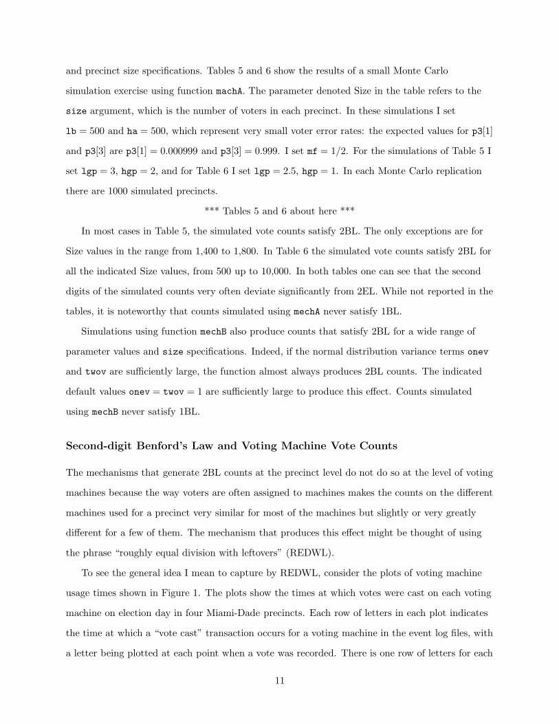
To see the general idea I mean to capture by REDWL, consider the plots of voting machine
usage times shown in Figure 1. The plots show the times at which votes were cast on each voting
machine on election day in four Miami-Dade precincts. Each row of letters in each plot indicates
the time at which a “vote cast” transaction occurs for a voting machine in the event log files, with
a letter being plotted at each point when a vote was recorded. There is one row of letters for each
11

voting machine used in each precinct. Times are shown using a 24-hour clock and resolved to the
second. In precinct 109, most of the machines were used throughout the day, but the machine
labeled “e” was not used after 10am, and the machine labeled “k” was used much less often in the
afternoon than in the morning. A reasonable guess is that the machine was pulled from service at
that time. In precinct 233, the machine labeled “c” was not used after 8am, and the machine
labeled “f” was not used before 2pm. In precinct 322, the machine labeled “b” was used only
between 11:30am and 2:30pm. In precinct 326, the machines labeled “g” and “m” were used only
after 1pm, and the machine labeled “p” was used heavily only after 6pm.
*** Figure 1 about here ***
These and other plots of machine usage times I have examined suggest the machines might be
separated into two categories, namely machines that are fully occupied pretty much throughout
election day versus the rest. The set of machines that are not fully occupied throughout the day
might be further subdivided into a set that is used heavily during some periods but only
sporadically at other times, and a set that is not use at all throughout much of election day. In
any case, REDWL reflects the idea that most of the votes in a precinct are recorded on a subset
of the machines, with the votes being roughly equally distributed among those machines, while
the remaining votes are scattered among the rest of the machines. A minimal indicator that
REDWL is a concern is that the total number of votes cast on some machines is similar among
the machines and noticeably higher (or lower) than the number cast on the rest of the machines.
A simple modification of one of the mechanisms previously seen to generate precinct-level 2BL
counts illustrates how the REDWL mechanism tends to produce voting machine counts that do
not satisfy 2BL, even when the process that is taking place in the precinct as a whole does
produce 2BL counts. Consider the following augmented version of mechA:
mechAm <- function(size, nprecincts=500, mf=1/3, lgp=1, hgp=1, lb=4, ha=4) {
lgb <- exp(lgp)/(exp(lgp)+exp(hgp)+1);
hgb <- exp(hgp)/(exp(lgp)+exp(hgp)+1);
mgb <- 1/(exp(lgp)+exp(hgp)+1);
pb <- ceiling(size/250);
sapply(1:nprecincts, function(x){
p3 <- c( rbeta(1,1/2,lb), mf, rbeta(1,ha,1/2) );
q <- runif(1,0,1);
pf <- c(q*lgb, mgb, (1-q)*hgb );
sumv <- sum(size * p3 * pf/sum(pf))
12

# allocate votes to the pb machines
mbeta <- rbeta(pb, 20,20*pb);
mbmean <- 1/(pb+1);
mtrunc <- ifelse(mbeta < mbmean, mbeta, mbmean);
sumv * mtrunc/sum(mtrunc);
})
}
The sumv values are precinct counts generated exactly as in mechA. The votes for the alternative
in each precinct are divided among pb machines, where pb is determined as a function of the size
of each precinct. There is roughly one machine for every 250 voters. In each precinct, pb random
(Beta-distributed) values mbeta are generated, where the expected value of mbeta is
mbmean = 1/(1 + pb). Values of mbeta greater than mbmean are set equal to the mean value, while
values of mbeta smaller than mbmean are left unchanged. Each precinct’s votes for the alternative
are assigned to voting machines in proportion to this vector of truncated values.
Running a small Monte Carlo simulation exercise using function machAm with the same
parameters that were used to compute the simulations reported in Table 6 shows that the
REDWL mechanism in most cases destroys the 2BL property of the simulated counts. Results of
this simulation are reported in Table 7. In contrast to the results in Table 6, the results in Table
7 show departures from 2BL for most precinct sizes. The only exceptions are for Size values
size = 500 and size = 700. Running the simulation with different numbers of voting machines
per voter does not materially change the results. Similar results are also obtained if the largest
machine counts are not constrained to be exactly the same. For instance, we get similar results if
instead of defining
mtrunc <- ifelse(mbeta < mbmean, mbeta, mbmean);
we use
mtrunc <- ifelse(mbeta < mbmean, mbeta, runif(pb,.95*mbmean,mbmean));
In this case the top machine proportions do not all have the value mbmean but instead vary
uniformly on the interval [.95 ∗ mbmean, mbmean].
*** Table 7 about here ***
I conclude from such demonstrations that while under normal circumstances we might expect
vote counts from precincts to satisfy 2BL, we should not expect vote counts from voting machines
13

to do so, if several voting machines are typically used in each precinct and if the total number of
votes cast on each machine exhibits signs of the REDWL mechanism.
Can the Second-digit Benford’s Law Detect Election Fraud?
Do relatively large X2B2
values for precinct-level vote counts suggest the counts have been
fraudulently manipulated? The simulations reported in Tables 5 and 6 suggest that an electorally
intelligible and benign process can produce counts that often satisfy the 2BL. Suppose we take a
process that we know usually produces such counts and perturb it in ways that mimic some ways
vote fraud may occur. Does the 2BL test signal that there has been a distortion? If so, we might
conclude that the relatively large X2B2
values suggest that maybe there has been fraud. Because
significant perturbations may occur in the absence of fraud, such a result can do no more than
suggest the possibility of fraud. But if the 2BL test does not catch perturbations that we inject
into otherwise pristine data, then of course the test is not useful for detecting vote fraud. In this
case clean precinct-level results should not give us any comfort.
I present illustrative simulations regarding 12 kinds of manipulations of vote counts. The
simulations use a rubric of votes being switched from one candidate to the another, although the
vote-switching perspective is not necessary for the results to be meaningful. In cases where a
candidate is simulated as gaining votes, the added votes might in some cases be considered not to
come from another candidate but simply to be introduced independent of anything that is
happening to other candidates’ votes. Such a reinterpretation may be especially appropriate in
relation to the simulations that use what I refer to as “repeaters,” because in those cases the
number of votes being added does not depend on the number of votes the other candidates are
receiving. In cases where a candidate is simulated as losing votes, the added votes might be
considered as simply disappearing. This might correspond to situations where there are
intentionally or accidentally spoiled or lost ballots.
Table 8 gives an overview of the simulated manipulations. The simulations all feature two
candidates in a simulated election where the expected outcome is a tie. Votes may be added to or
subtracted from a candidate, with consequently the same number of votes being subtracted from
or given to the other candidate. The vote shifts may occur in all precincts, only in those precincts
where the first affected candidate receives more votes than expected or only in those precincts
14

where the first affected candidate receives fewer votes than expected. The votes the first affected
candidate receives (or loses) may be either a proportion of the votes the other candidate would
otherwise have received or a proportion of the total number of voters in the precinct. These latter
cases are the ones I describe as having “repeaters.”
*** Table 8 about here ***
My conception of repeaters harks back to the classic manipulation Gumbel (2005) describes as
having been perfected by several American city political machines in the late nineteenth and early
twentieth centuries. Repeaters in the nineteenth century’s Tammany Hall were the primary
referents of the familiar phrase, “vote early and often.” As Gumbel writes, “The repeaters carried
changes of clothing, including several sets of coats and hats, so they could plausibly come forward
a second or third or fourth time in the guise of an entirely new person.... Many of the repeaters
sported full beards at the beginning of the day, only to end it clean-shaven” (Gumbel 2005, 74).
Nowadays repeaters might simply be a few lines of computer code.
The simulations are based on the first mechanism that produces 2BL counts. The following R
function gives the simulations’ typical form.
mechA2p <- function(size, nprecincts=500, mf=1/3, lgp=1, hgp=1, lb=4, ha=4, fa=0) {
mp <- meanAp(lgp=lgp, hgp=hgp, mf=mf, lb=lb, ha=ha);
lgb <- exp(lgp)/(exp(lgp)+exp(hgp)+1);
hgb <- exp(hgp)/(exp(lgp)+exp(hgp)+1);
mgb <- 1/(exp(lgp)+exp(hgp)+1);
sapply(1:nprecincts, function(x){
p3mat <- matrix(c(rbeta(1,1/2,lb), mf, rbeta(1,ha,1/2),
rbeta(1,ha,1/2), mf, rbeta(1,1/2,lb)),
2, 3, byrow=TRUE );
p3mat <- apply(p3mat,2,function(v){ ifelse(sum(v)>c(1,1), v/sum(v), v) });
p3 <- c( rbeta(1,1/2,lb), mf, rbeta(1,ha,1/2) );
q <- runif(1,0,1);
pf <- c(q*lgb, mgb, (1-q)*hgb );
y <- c(size*p3mat %*% pf/sum(pf));
chg <- ifelse(y[1] > size*mp, fa*y[2], 0);
y <- y + c(chg,-chg);
ifelse(y < 0, 0, y);
})
}
For each simulated precinct the function computes vote counts for two candidates, the votes for
each having the attributes of counts produced by mechA. A function meanAp computes the
15

proportion of the votes the first candidate is expected to receive, and the resulting expectation is
assigned to mp. The line
chg <- ifelse(y[1] > size*mp, fa*y[2], 0);
defines a change value for each precinct that equals a proportion fa times the votes received by
the second candidate if the first candidate’s vote count is greater than the expected count
size*mp, and otherwise the change value equals zero. In the case where the vote shifts occur in
all precincts, the expectation is ignored and the change value is defined by
chg <- fa*y[2];
The value fa*y[2] corresponds to the proportional vote switch scenario. For the repeater
scenario that value is replaced with fa*size. To define a simulated election that would be
expected to be a tie (i.e., very close) in the absence of any manipulations, I set the parameter
values size = 2500, lgp = 2, hgp = 2, mf = 1/3, lb = 4 and ha = 4.
The first set of results, reported in Table 9, shows what happens when votes are
proportionally added to the first candidate in all precincts. I present results for, respectively, 500,
1,000 and 2,000 simulated precincts. The fraction of votes shifted ranges from zero (no
manipulation) to a substantial fa = .15. In this scenario the 2BL test does not detect that votes
have been added to the first candidate. The 2BL test starts to signal the losses being suffered by
the second candidate only when they are fairly substantial and the number of precincts is large.
With 2,000 precincts and a switched fraction of seven percent or smaller, the average of X 2B2
is
smaller than the critical value for χ29 for a test at level α = .05, which is 16.9. But X2
B2is
expected to exceed that critical value if fa ≥ .08.
*** Table 9 about here ***
Table 10 shows that having the proportional additions occur only in precincts where the first
candidate’s support is either particularly strong or particularly weak makes the vote switching
much more susceptible to detection by the 2BL test. With 2,000 precincts, the 2BL test tends to
be triggered by the first candidate’s vote counts when as few as three percent of the votes are
being switched. With 500 precincts the 2BL test tends to be triggered when six or seven percent
of the votes are being switched. Tests of the second candidate’s vote counts are substantially less
16

sensitive when the votes are being taken from that candidate in precincts where the other
candidate is strong, and somewhat less sensitive when the votes are being taken in precincts
where the other candidate is weak.
*** Table 10 about here ***
Table 11 shows that the 2BL detectability of repeater additions in all precincts is similar to
the detectability of proportional additions. But in Table 12 it is apparent that repeater additions
that occur in the first candidate’s areas of either relative strength or relative weakness are more
readily detected than the corresponding proportional additions are. With 2,000 precincts,
switching as little as two percent of the vote in the affected precincts tends to produce X 2B2
values
for the first candidate’s vote counts that are greater than the α = .05 critical value for χ29. Tests
of the second candidate’s vote counts are somewhat less sensitive.
*** Tables 11 and 12 about here ***
Table 13 shows that proportional substractions in all precincts are if anything slightly less
detectable than the corresponding proportional additions are. Even with 2,000 precincts, such
subtractions do not tend to produce large X2B2
values for either candidate. As Table 14 shows,
however, having the proportional subtractions occur only in precincts where the first candidate’s
support is either particularly strong or particularly weak makes the vote switching much more
susceptible to detection. With 2,000 precincts, the 2BL test triggers with as little as a two
percent subtraction from the counts in the first candidate’s strongest precincts.
*** Tables 13 and 14 about here ***
Tables 15 and 16 show that the 2BL detectability of repeater substractions is comparable to
that of repeater additions. Indeed, Table 16 shows that with 2,000 precincts a repeater
subtraction amounting to one percent of the voters is detectable by a 2BL test of the first
candidate’s vote counts, if the first candidate’s strongest precincts are the ones affected.
Detectability is only slightly less when the manipulations are directed at the first candidate’s
weakest precincts.
*** Tables 15 and 16 about here ***
On the whole the simulations suggest that the 2BL test can be highly sensitive to additions or
subtractions from candidates’ precinct-level vote totals. Sensitivity in the considered scenario of
an extremely close election is generally weaker when manipulations equally affect all precincts.
17

For such pervasive changes in vote counts, the 2BL test is sometimes not at all sensitive given the
number of precincts considered here. But when manipulations are concentrated in either one
candidate’s strongest or weakest precincts, the 2BL test can produce significant results when even
very small shares of the vote are switched. In some instances, with 2,000 precincts, changes are
detectable when they are as small as one or two percent of either the votes the other candidate
received or the number of voters in each precinct. The 2BL test can in this sense sometimes—not
always—detect changes in vote counts that are just large enough to change the outcome of a very
close election.
More Data from Florida 2004
Data from the 2004 election in other Florida counties repeat the patterns found for Miami-Dade.
Table 17 provides an overview of the kind of data to be considered. The table shows the number
of precincts in Miami-Dade, Broward and Pasco counties. In 2004, Miami-Dade, Broward and
Pasco counties all used Election Systems & Software “iVotronic” electronic voting machines (see
Electronic Frontier Foundation (2004)). On election day, some voting machines were used to
record votes from more than one precinct. This occurred in cases where more than one precinct
shared a polling place. Most voting occurred on election day, November 2, 2004, but votes were
also cast during a 15-day early voting period (October 18 through November 1, 2004). Table 17
also shows the number of early voting sites used in each county (earlyvoting.org 2004;
Miami-Dade County 2004; Browning 2004). In Broward and Pasco, voters from all precincts could
vote at any early voting site. In Miami-Dade, voters from each precinct could vote only at
selected early voting locations. At early voting sites in Miami-Dade, each voting machine was
used for voters from multiple precincts. The voting data for the early voting period do not
directly indicate the voter’s precinct but instead indicate which of several ballot styles the voter
used. Table 17 shows the number of styles used during early voting for each county. The event log
files do not contain any indication of the physical location where each voting machine was used
during the early voting period. I use Personal Electronic Ballot (PEB)4 codes recorded in the
event log files to group machines together, the idea being that machines for which the same PEB
4For a description of how PEBs are used in Election Systems & Software “iVotronic” voting machines, see (Elec-tronic Frontier Foundation 2004).
18

was used must have been located at the same early voting site.
*** Table 17 about here ***
A concern with early voting is that not every voting machine was used every day during the
early voting period. I use the event log files to identify the dates during the early voting period
when each voting machine was used. I group machines together only if they were used on all the
same days. The “site-days” entries in Table 17 show the number of unique combinations of the
PEB-based location groupings with these date goupings in Broward and Pasco, and the
“style-site-days” entry shows the number of unique combinations of the PEB-based location and
ballot style groupings with the date goupings in Miami-Dade. These serve as the “precincts” for
the early voting vote counts. The “site-day-machines” and “s-s-d-machines” (for
“site-style-day-machines”) entries show the number of unique combinations of the site-days or
style-site-days groupings with voting machines.
Applying the 2BL test to other vote count data from the 2004 election in Florida mostly
suggests that 2BL applies to the data, but a few results raise questions. Table 18 reports results
based on data from early voting in Miami-Dade. Applying the FDR to the twenty tests for
site-style-days, the results look fine if we use a single-test level of α = .05, since no X 2B2
value is
greater than 25.46, but the results are problematic if α = .10: X 2B2
for the Amendment 7 Yes
votes is 24.6, which is greater than 23.6. The election day precinct results for Broward, shown in
Table 19, are similar. They are fine using the FDR with α = .05 but problematic using α = .10:
two of the Amendment vote counts have X2B2
> 23.6. The Broward early voting results for counts
at the level of ballot styles are fine if the FDR is used. The largest X 2B2
value among these early
voting tests is X2B2
= 21.4, for the votes for Kerry. The election day results for Pasco, shown in
Table 20, have one value of X2B2
large enough to reject the hypothesis that 2BL applies even using
the FDR among the twenty tests with α = .05. This is the value X 2B2
= 29.5, which occurs for the
Amendment 7 Yes votes. Considered on their own and using the FDR for twenty tests, the early
voting machine-precinct results for Pasco are fine.
*** Tables 18, 19 and 20 about here ***
The results for voting machines in Tables 18, 19 and 20 further illustrate that the 2BL
property mostly does not apply to the vote counts on machines in these Florida counties. The
case that comes closest to being an exception is the machine results for early voting in Broward.
19
Many of those X2B2
values are unproblematically small, but three are larger than the χ29 critical
value for a single test at level α = .05, and two are large even when we use the FDR. For the
Amendment 8 Yes votes we have X2B2
= 27.9, which is larger than the critical value for the FDR
for twenty tests with α = .05, and for the Amendment 7 Yes votes we have X 2B2
= 44.0, which is
very large by any standard.
The value X2B2
= 29.5 that occurs for the election day precinct data from Pasco is large
enough to count as a rejection of the 2BL hypothesis even using the FDR among all 60 of the
election day tests, pooling across the three counties: the quantile of χ29 corresponding to a tail
probability of .05/60 is 28.35. Pooling over all 120 of the election day precinct and early voting
site-style-day, style and machine-precinct tests, the value X 2B2
= 29.5 is not problematic according
to the FDR with α = .05, since the quantile of χ29 corresponding to a tail probability of .05/120 is
30.13. But using α = .10 we again have a problem even when pooling over all 120 tests, because
using the FDR we again arrive at the χ29 quantile of 28.35.
Data from Mexico 2006
The 2006 election in Mexico has proven to be highly controversial. A very close outcome between
the top two finishers in the presidential election led to calls from Democratic Revolution Party
(PRD) candidate Andres Manuel Lopez Obrador for a manual recount of all 41 million ballots.
The declared winner, National Action Party (PAN) candidate Felipe Calderon, officially has
15,000,284 votes while Lopez Obrador has 14,756,350. As of the time of this writing Calderon has
declared willingness to support a recount if that is ordered by the Federal Electoral Tribunal
(TRIFE), but expresses doubt that the results would change or that a recount of all the ballots is
in any case necessary (Associated Press 2006b,a). Other parties receiving votes in the election
include the Institutional Revolutionary Party (PRI), the Social-Democratic and Rural Alternative
Party (ASDC) and the New Alliance Party (NA). In the presidential voting these parties received,
respectively, 9,301,441 (22.3 percent), 1,127,963 (2.7 percent) and 401,804 (1.0 percent) votes.
Here I present 2BL test results for votes at two levels of aggregation, “secciones,” which
correspond to precincts, and “casillas,” which correspond to voting machines.5 The Mexican
5I downloaded official vote count data from the website of the Instituto Federal Electoral (IFE),http://www.ife.org.mx/, on July 13, 2006.
20

election used paper ballots, so these “machines” in fact correspond to the boxes into which voters
placed their ballots. Typically there are multiple casillas for each seccion. In each seccion voters
are assigned to casillas based on each voter’s name, not haphazardly as often occurs in elections
in the United States. Inspecting the total numbers of ballots cast at each casilla shows patterns
that suggest the REDWL mechanism should be a concern. Hence the 2BL test is likely to be
appropriate for seccion-level vote counts but not for casilla-level counts.
Table 21 shows seccion-level 2BL test results. The first row of the table reports results
considering all the secciones from across the whole country as one set. The X 2B2
statistics are
larger than the χ29 critical value for test level α = .05 for four of the five parties. For ASDC the
statistic is larger than the critical value for test level α = .1. The remaining rows of the table
show results separately for the secciones in each of Mexico’s 32 states. In this case, taking into
account the FDR for 32 separate tests gives an adjusted critical value of 26.7 for level α = .05 and
a value of 24.9 for level α = .1. The FDR for all 160 separate tests gives critical values of 30.9 and
29.1 respectively for levels α = .05 and α = .1. For each party there are X 2B2
statistics larger than
these FDR-adjusted critical values. For the two largest parties areas in Mexico city (the state
Mexico) are particularly problematic, but a few other areas also show high values for X 2B2
.
Notably, for all but the smallest party (NA), most of the X 2B2
values are smaller than even the
single-test critical values.
*** Table 21 about here ***
Table 22 shows that an analysis at the casilla level conveys a very different impression. Now
most of the X2B2
values are large. The difference between the 2BL tests for the casilla and seccion
vote counts mirrors the difference observed in the Florida counties between the voting machine
and precinct vote counts. In both cases the REDWL mechanism is the most likely explanation for
why the lower level of aggregation produces systematically worse results. The worse casilla results
therefore probably do not signal more widespread or more serious problems than the seccion-level
results do.
*** Table 22 about here ***
The 2BL test results for secciones certainly suggest there are problems with the 2006
presidential vote counts in many Mexican states, although probably not in most of them. More
refined analysis is needed to reach sharper conclusions, but the general impression is that more
21
intensive investigation of the election results is in order. That might include doing a manual
recount of many—perhaps all—of the individual ballots. A cost efficient method may be to begin
by recounting a random sample of the ballots—all the ballots in a sample of secciones—where the
probability that a seccion is selected for recounting is greater in places where the 2BL test results
are worse. For such an exercise it may be reasonable to conduct 2BL tests for secciones collected
into sets that correspond to the legislative districts they are part of, with sampling for purposes of
initial recounting done at the level of districts. Perhaps a two-stage sampling plan could be used,
with districts selected at the first stage (weighted by the 2BL test results) and secciones within
each district selected at the second stage. If such an initial sampling did identify problems with
the vote tabulations, then the case for a comprehensive manual recount would become extremely
strong.
Discussion
Tests based on the second-digit Benford’s Law show strong promise to become a standard tool for
detecting fraudulent election results. The 2BL test cannot detect all kinds of fraud, and significant
2BL test results may occur even when vote counts are in no way fraudulent. But one should
perhaps not expect too much from a test that has only the vote counts themselves to work with.
An important apparent limitation of the 2BL test is that it seems not to be suitable for
checking voting machine level counts, at least not when the way voters are assigned to machines
brings the REDWL mechanism into play. An idea worth investigation is whether strict random
assignment of voters to machines can avoid the REDWL mechanism, so that 2BL tests would be
informative at the level of individual voting machine counts. The few simulations I have
conducted so far suggest that such an approach might be effective.
Data Note
David Dill supplied ballot and event log files recovered from electronic voting machines in
Broward, Miami-Dade and Pasco counties. The files were originally obtained by Martha
Mahoney. The ballot files indicate the choices made for each office by each voter and include
labels identifying for each ballot the voting machine and the precinct (for election day ballots) or
ballot style (for early voting ballots). The event log files show the time (resolved to the second) at
22
which various transactions occurred on each machine, including the time at which each vote was
recorded. It is not possible to match vote choices in the ballot files to voting events in the event
log files.
Early voting polling site locations for many of the Miami-Dade machines was taken from a file
supplied by Martha Mahoney (file “ev.xls,” received by me on August 16, 2005) that was
obtained using open records requests funded by the Verified Voting Foundation. Of the 670
machines that recorded votes during early voting in Miami-Dade, 88 are not included in that file.
Two files supplied by Martha Mahoney also were used to determine which Miami-Dade machines
were operating with audio capability enabled. These are the “ev.xls” file and a file “Election.xls”
(received by me on August 16, 2005) for the machines used on election day.
The data comprise files for electronic early voting and electronic polling place votes but do not
include information about paper absentee votes.
23

References
Associated Press. 2006a. “Disputed Election Leaves Mexico Adrift.” Associated Press. July 15.
Associated Press. 2006b. “Lopez Obrador Widens Election Fraud Claims.” Associated Press. July
13.
Benjamini, Yoav and Yosef Hochberg. 1995. “Controlling the False Discovery Rate: A Practical
and Powerful Approach to Multiple Testing.” Journal of the Royal Statistical Society, Series B
57 (1): 289–300.
Benjamini, Yoav and Daniel Yekutieli. 2005. “False Discovery Rate-Adjusted Multiple Confidence
Intervals for Selected Parameters.” Journal of the American Statistical Association 100 (Mar.):
71–81.
Brady, Henry E. 2005. “Comments on Benford s Law and the Venezuelan Election.” MS dated
January 19, 2005.
Browning, Kurt S. 2004. “Vote Notes.” Quarterly Publication of the Pasco County Supervisor of
Elections.
Carter Center. 2005. “Observing the Venezuela Presidential Recall Referendum: Comprehensive
Report.”.
Durtschi, Cindy, William Hillison, and Carl Pacini. 2004. “The Effective Use of Benford’s Law to
Assist in Detecting Fraud in Accounting Data.” Journal of Forensic Accounting 5: 17–34.
earlyvoting.org. 2004. “Early Voting for Broward Voters in the November 2, 2004 General Election.”
URL http://earlyvoting.org/earlyvoting14sites.pdf (accessed January 20, 2006).
Electronic Frontier Foundation. 2004. “Electronic Voting Machine Information Sheet:
Election Systems & Software iVotronic.” URL http://www.eff.org/Activism/E-
voting/20040818 ess ivotronic v0.8.pdf (accessed March 27, 2006).
Gronke, Paul, Benjamin Bishin, Daniel Stevens, and Eva Galanes-Rosenbaum. 2005. “Early Voting
in Florida, 2004.” Paper prepared for the Annual Meeting of the American Political Science
Association, Washington, DC, September 1, 2005.
24
Gumbel, Andrew. 2005. Steal This Vote. New York: Nation Books.
Hill, Theodore P. 1995. “A Statistical Derivation of the Significant-digit Law.” Statistical Science
10: 354–363.
Janvresse, Elise and Thierry de la Rue. 2004. “From Uniform Distributions to Benford’s Law.”
Journal of Applied Probability 41: 1203–1210.
Lehoucq, Fabrice. 2003. “Electoral Fraud: Causes, Types, and Consequences.” Annual Review of
Political Science 6 (June): 233–256.
Mebane, Walter R., Jr. and Jasjeet S. Sekhon. 2004. “Robust Estimation and Outlier Detection
for Overdispersed Multinomial Models of Count Data.” American Journal of Political Science
48 (Apr.): 392–411.
Mebane, Walter R., Jr., Jasjeet S. Sekhon, and Jonathan Wand. 2001. “Detection of Multinomial
Voting Irregularities.” 2001 Proceedings of the American Statistical Association. Social Statistics
Section [CD-ROM].
Miami-Dade County. 2004. “New, Expanded Hours Announced for Early Voting in Hialeah as
Miami-Dade County Sets New Early Voting Record.” News release, October 21, 2004.
Pericchi, Luis Raul and David Torres. 2004. “La Ley de Newcomb-Benford y sus aplicaciones
al Referendum Revocatorio en Venezuela.” Reporte Tecnico no-definitivo 2a. version: Octubre
01,2004.
R Development Core Team. 2003. R: A Language and Environment for Statistical Computing . R
Foundation for Statistical Computing. Vienna, Austria. ISBN 3-900051-00-3.
URL http://www.R-project.org
Raimi, Ralph A. 1976. “The First Digit Problem.” American Mathematical Monthly 83 (7): 521–
538.
Taylor, Jonathan. 2005. “Too Many Ties? An Empirical Analysis of the Venezuelan Referendum
Counts.” MS dated November 7, 2005.
25

Wand, Jonathan, Kenneth Shotts, Jasjeet S. Sekhon, Walter R. Mebane, Jr., Michael Herron, and
Henry E. Brady. 2001. “The Butterfly Did It: The Aberrant Vote for Buchanan in Palm Beach
County, Florida.” American Political Science Review 95 (Dec.): 793–810.
26

Table 1: Frequency of Digits according to Benford’s Law
digit 0 1 2 3 4 5 6 7 8 9first — .301 .176 .124 .097 .079 .067 .058 .051 .046second .120 .114 .109 .104 .100 .097 .093 .090 .088 .085
Table 2: Florida Constitutional Amendments on the Ballot in 2004
Yes NoAm. 1 Parental Notification of a Minor’s Termination of Pregnancy 4,639,635 2,534,910Am. 2 Constitutional Amendments Proposed by Initiative 4,574,361 2,109,013Am. 3 The Medical Liability Claimant’s Compensation Amendment 4,583,164 2,622,143Am. 4 Authorizes Miami-Dade and Broward County Voters to Ap-
prove Slot Machines in Parimutuel Facilities3,631,261 3,512,181
Am. 5 Florida Minimum Wage Amendment 5,198,514 2,097,151Am. 6 Repeal of High Speed Rail Amendment 4,519,423 2,573,280Am. 7 Patients’ Right to Know About Adverse Medical Incidents 5,849,125 1,358,183Am. 8 Public Protection from Repeated Medical Malpractice 5,121,841 2,083,864
Note: Yes and No vote counts show statewide results.
27

Table 3: Miami-Dade Election Day First-digit Benford’s Law Tests
item Benf. equal item Benf. equal
Bush 29.3 292.5 Am. 4 Yes 144.8 367.0Kerry 39.9 287.0 Am. 4 No 119.6 605.6Martinez 35.6 273.8 Am. 5 Yes 115.4 122.2Castor 22.0 304.7 Am. 5 No 27.6 623.4Am. 1 Yes 86.2 290.5 Am. 6 Yes 98.8 395.0Am. 1 No 80.5 636.2 Am. 6 No 84.0 532.9Am. 2 Yes 95.6 362.5 Am. 7 Yes 130.3 112.7Am. 2 No 60.0 722.7 Am. 7 No 49.9 582.8Am. 3 Yes 60.5 401.3 Am. 8 Yes 123.0 210.6Am. 3 No 51.5 496.5 Am. 8 No 102.6 831.1
Note: n = 757 precincts. Each statistic is the Pearson chi-squared statistic, with eight degrees offreedom.
28
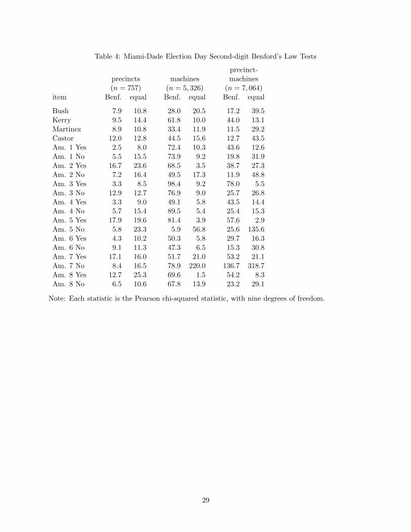
Table 4: Miami-Dade Election Day Second-digit Benford’s Law Tests
precinct-precincts machines machines(n = 757) (n = 5, 326) (n = 7, 064)
item Benf. equal Benf. equal Benf. equal
Bush 7.9 10.8 28.0 20.5 17.2 39.5Kerry 9.5 14.4 61.8 10.0 44.0 13.1Martinez 8.9 10.8 33.4 11.9 11.5 29.2Castor 12.0 12.8 44.5 15.6 12.7 43.5Am. 1 Yes 2.5 8.0 72.4 10.3 43.6 12.6Am. 1 No 5.5 15.5 73.9 9.2 19.8 31.9Am. 2 Yes 16.7 23.6 68.5 3.5 38.7 27.3Am. 2 No 7.2 16.4 49.5 17.3 11.9 48.8Am. 3 Yes 3.3 8.5 98.4 9.2 78.0 5.5Am. 3 No 12.9 12.7 76.9 9.0 25.7 26.8Am. 4 Yes 3.3 9.0 49.1 5.8 43.5 14.4Am. 4 No 5.7 15.4 89.5 5.4 25.4 15.3Am. 5 Yes 17.9 19.6 81.4 3.9 57.6 2.9Am. 5 No 5.8 23.3 5.9 56.8 25.6 135.6Am. 6 Yes 4.3 10.2 50.3 5.8 29.7 16.3Am. 6 No 9.1 11.3 47.3 6.5 15.3 30.8Am. 7 Yes 17.1 16.0 51.7 21.0 53.2 21.1Am. 7 No 8.4 16.5 78.9 220.0 136.7 318.7Am. 8 Yes 12.7 25.3 69.6 1.5 54.2 8.3Am. 8 No 6.5 10.6 67.8 13.9 23.2 29.1
Note: Each statistic is the Pearson chi-squared statistic, with nine degrees of freedom.
29
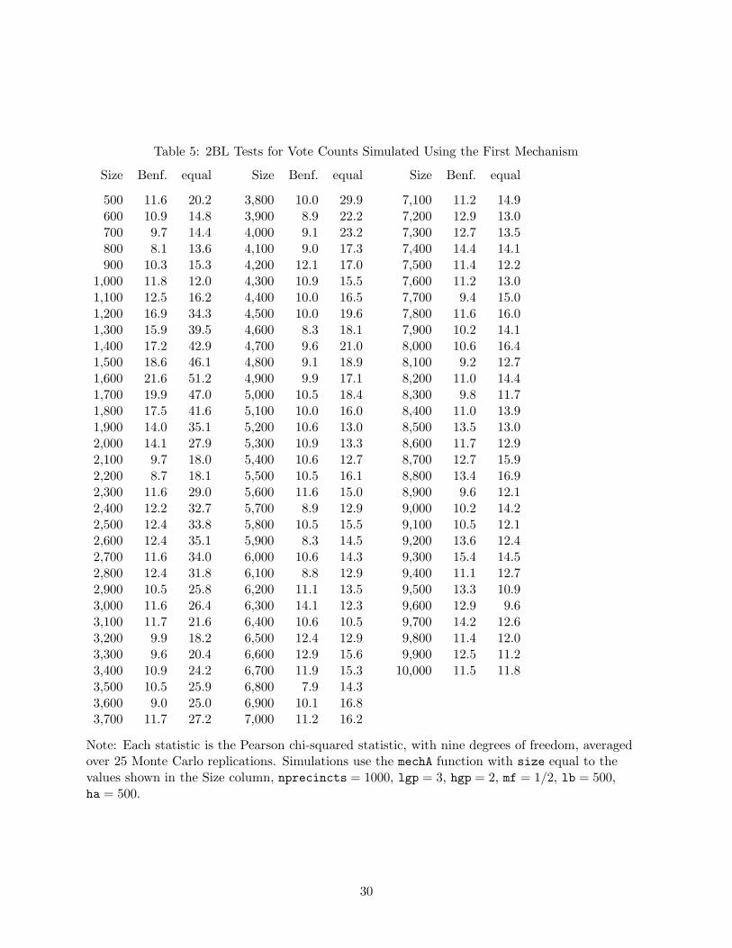
Table 5: 2BL Tests for Vote Counts Simulated Using the First Mechanism
Size Benf. equal Size Benf. equal Size Benf. equal
500 11.6 20.2 3,800 10.0 29.9 7,100 11.2 14.9600 10.9 14.8 3,900 8.9 22.2 7,200 12.9 13.0700 9.7 14.4 4,000 9.1 23.2 7,300 12.7 13.5800 8.1 13.6 4,100 9.0 17.3 7,400 14.4 14.1900 10.3 15.3 4,200 12.1 17.0 7,500 11.4 12.2
1,000 11.8 12.0 4,300 10.9 15.5 7,600 11.2 13.01,100 12.5 16.2 4,400 10.0 16.5 7,700 9.4 15.01,200 16.9 34.3 4,500 10.0 19.6 7,800 11.6 16.01,300 15.9 39.5 4,600 8.3 18.1 7,900 10.2 14.11,400 17.2 42.9 4,700 9.6 21.0 8,000 10.6 16.41,500 18.6 46.1 4,800 9.1 18.9 8,100 9.2 12.71,600 21.6 51.2 4,900 9.9 17.1 8,200 11.0 14.41,700 19.9 47.0 5,000 10.5 18.4 8,300 9.8 11.71,800 17.5 41.6 5,100 10.0 16.0 8,400 11.0 13.91,900 14.0 35.1 5,200 10.6 13.0 8,500 13.5 13.02,000 14.1 27.9 5,300 10.9 13.3 8,600 11.7 12.92,100 9.7 18.0 5,400 10.6 12.7 8,700 12.7 15.92,200 8.7 18.1 5,500 10.5 16.1 8,800 13.4 16.92,300 11.6 29.0 5,600 11.6 15.0 8,900 9.6 12.12,400 12.2 32.7 5,700 8.9 12.9 9,000 10.2 14.22,500 12.4 33.8 5,800 10.5 15.5 9,100 10.5 12.12,600 12.4 35.1 5,900 8.3 14.5 9,200 13.6 12.42,700 11.6 34.0 6,000 10.6 14.3 9,300 15.4 14.52,800 12.4 31.8 6,100 8.8 12.9 9,400 11.1 12.72,900 10.5 25.8 6,200 11.1 13.5 9,500 13.3 10.93,000 11.6 26.4 6,300 14.1 12.3 9,600 12.9 9.63,100 11.7 21.6 6,400 10.6 10.5 9,700 14.2 12.63,200 9.9 18.2 6,500 12.4 12.9 9,800 11.4 12.03,300 9.6 20.4 6,600 12.9 15.6 9,900 12.5 11.23,400 10.9 24.2 6,700 11.9 15.3 10,000 11.5 11.83,500 10.5 25.9 6,800 7.9 14.33,600 9.0 25.0 6,900 10.1 16.83,700 11.7 27.2 7,000 11.2 16.2
Note: Each statistic is the Pearson chi-squared statistic, with nine degrees of freedom, averagedover 25 Monte Carlo replications. Simulations use the mechA function with size equal to thevalues shown in the Size column, nprecincts = 1000, lgp = 3, hgp = 2, mf = 1/2, lb = 500,ha = 500.
30

Table 6: 2BL Tests for Vote Counts Simulated Using the First Mechanism
Size Benf. equal Size Benf. equal Size Benf. equal
500 10.3 22.5 3,800 11.3 18.7 7,100 8.3 15.7600 9.5 18.1 3,900 9.2 17.7 7,200 9.1 17.1700 10.0 15.7 4,000 12.2 19.6 7,300 8.9 19.6800 9.0 19.6 4,100 10.5 20.0 7,400 9.3 18.0900 10.0 13.2 4,200 10.4 19.5 7,500 7.8 18.1
1,000 9.7 15.7 4,300 9.1 18.4 7,600 7.9 18.11,100 10.4 13.4 4,400 10.2 16.1 7,700 9.1 22.01,200 12.0 15.9 4,500 12.3 17.5 7,800 10.9 21.11,300 12.3 27.2 4,600 9.9 14.4 7,900 8.7 17.61,400 13.4 35.2 4,700 11.2 20.0 8,000 9.0 17.71,500 13.8 35.5 4,800 9.6 20.9 8,100 11.4 17.41,600 13.9 38.6 4,900 8.6 21.7 8,200 9.1 16.91,700 15.4 42.8 5,000 8.8 22.6 8,300 10.4 14.81,800 14.0 38.2 5,100 9.1 25.2 8,400 9.1 16.21,900 13.6 37.0 5,200 9.7 23.1 8,500 9.1 14.82,000 12.4 34.4 5,300 10.5 27.0 8,600 9.5 17.52,100 10.7 27.2 5,400 9.2 24.1 8,700 9.6 13.82,200 9.3 21.9 5,500 10.1 20.9 8,800 9.9 14.92,300 8.1 18.6 5,600 10.9 17.2 8,900 9.3 14.92,400 10.5 24.0 5,700 9.8 15.8 9,000 9.2 14.12,500 11.2 27.7 5,800 9.2 16.6 9,100 10.2 14.72,600 9.4 30.0 5,900 9.6 15.2 9,200 11.0 13.92,700 12.3 31.7 6,000 9.2 15.4 9,300 10.0 15.22,800 12.4 29.3 6,100 8.3 16.9 9,400 10.2 13.92,900 12.9 29.6 6,200 9.2 17.3 9,500 8.1 14.33,000 13.3 26.8 6,300 8.9 16.0 9,600 10.8 20.33,100 11.6 23.3 6,400 9.9 14.4 9,700 9.7 15.53,200 13.0 23.4 6,500 10.8 16.6 9,800 10.1 16.43,300 12.3 16.7 6,600 11.1 17.3 9,900 9.5 16.03,400 11.4 15.2 6,700 8.8 15.3 10,000 10.2 18.23,500 12.4 11.7 6,800 8.8 17.33,600 12.7 16.9 6,900 10.0 14.73,700 9.9 18.7 7,000 8.7 15.6
Note: Each statistic is the Pearson chi-squared statistic, with nine degrees of freedom, averagedover 25 Monte Carlo replications. Simulations use the mechA function with size equal to thevalues shown in the Size column, nprecincts = 1000, lgp = 2.5, hgp = 1, mf = 1/2, lb = 500,ha = 500.
31

Table 7: 2BL Tests for Vote Counts Simulated Using the First Mechanism
Size Benf. equal Size Benf. equal Size Benf. equal
500 9.9 44.3 3,800 65.2 379.9 7,100 105.9 673.0600 22.0 80.4 3,900 53.5 345.3 7,200 106.8 668.5700 14.5 64.7 4,000 52.8 323.8 7,300 131.0 752.0800 27.8 113.1 4,100 79.7 430.9 7,400 119.3 699.6900 18.6 89.8 4,200 63.6 368.2 7,500 100.2 627.2
1,000 19.1 96.3 4,300 68.4 434.8 7,600 120.5 721.11,100 25.8 114.8 4,400 58.9 394.3 7,700 105.8 662.51,200 23.8 115.2 4,500 59.6 391.9 7,800 110.7 673.11,300 26.5 139.5 4,600 64.5 435.7 7,900 120.4 740.91,400 24.4 130.8 4,700 72.1 435.0 8,000 117.3 725.11,500 27.3 140.2 4,800 73.4 469.0 8,100 130.4 785.31,600 28.1 145.5 4,900 78.3 484.4 8,200 111.7 723.81,700 30.7 162.5 5,000 77.0 467.7 8,300 133.7 822.01,800 33.7 178.5 5,100 82.3 507.2 8,400 103.9 734.51,900 29.0 185.2 5,200 73.3 482.5 8,500 120.7 752.42,000 29.1 179.9 5,300 72.5 483.5 8,600 148.0 862.62,100 39.4 214.9 5,400 78.9 499.5 8,700 141.6 794.82,200 36.6 212.4 5,500 89.1 506.1 8,800 120.9 825.72,300 29.9 212.1 5,600 74.1 526.2 8,900 111.1 768.22,400 35.2 211.4 5,700 80.9 531.7 9,000 124.3 771.42,500 39.0 231.6 5,800 97.6 589.0 9,100 134.0 821.42,600 40.8 250.5 5,900 107.5 589.0 9,200 113.2 798.42,700 44.5 261.5 6,000 102.5 574.1 9,300 124.9 810.22,800 49.5 272.9 6,100 82.5 533.2 9,400 124.5 840.22,900 48.1 289.6 6,200 95.6 577.3 9,500 121.3 814.73,000 46.1 271.6 6,300 83.3 557.9 9,600 174.0 994.53,100 41.1 275.2 6,400 106.6 588.3 9,700 123.8 851.13,200 45.8 290.8 6,500 89.5 542.8 9,800 145.1 933.23,300 48.3 302.2 6,600 81.4 548.8 9,900 151.9 923.83,400 44.3 295.4 6,700 91.8 612.3 10,000 136.3 895.23,500 62.1 330.4 6,800 102.3 653.23,600 64.4 357.3 6,900 100.7 646.73,700 54.6 325.5 7,000 95.8 631.3
Note: Each statistic is the Pearson chi-squared statistic, with nine degrees of freedom, averagedover 25 Monte Carlo replications. Simulations use the mechAm function with size equal to thevalues shown in the Size column, nprecincts = 1000, lgp = 2.5, hgp = 1, mf = 1/2, lb = 500,ha = 500.
32
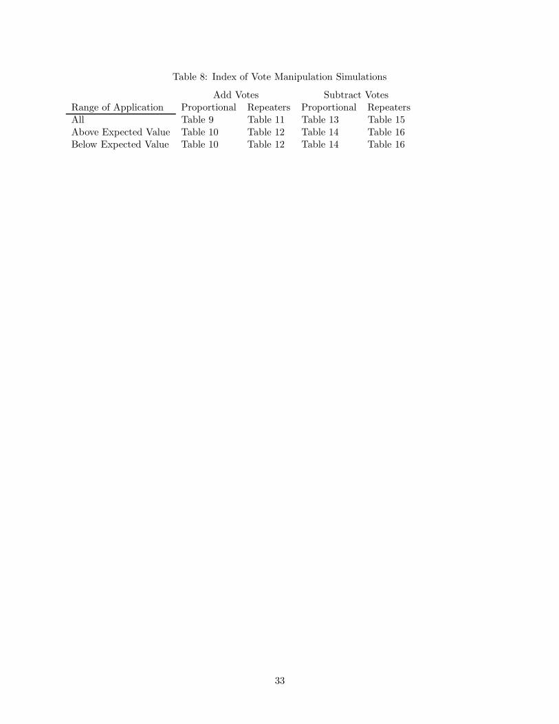
Table 8: Index of Vote Manipulation Simulations
Add Votes Subtract VotesRange of Application Proportional Repeaters Proportional RepeatersAll Table 9 Table 11 Table 13 Table 15Above Expected Value Table 10 Table 12 Table 14 Table 16Below Expected Value Table 10 Table 12 Table 14 Table 16
33
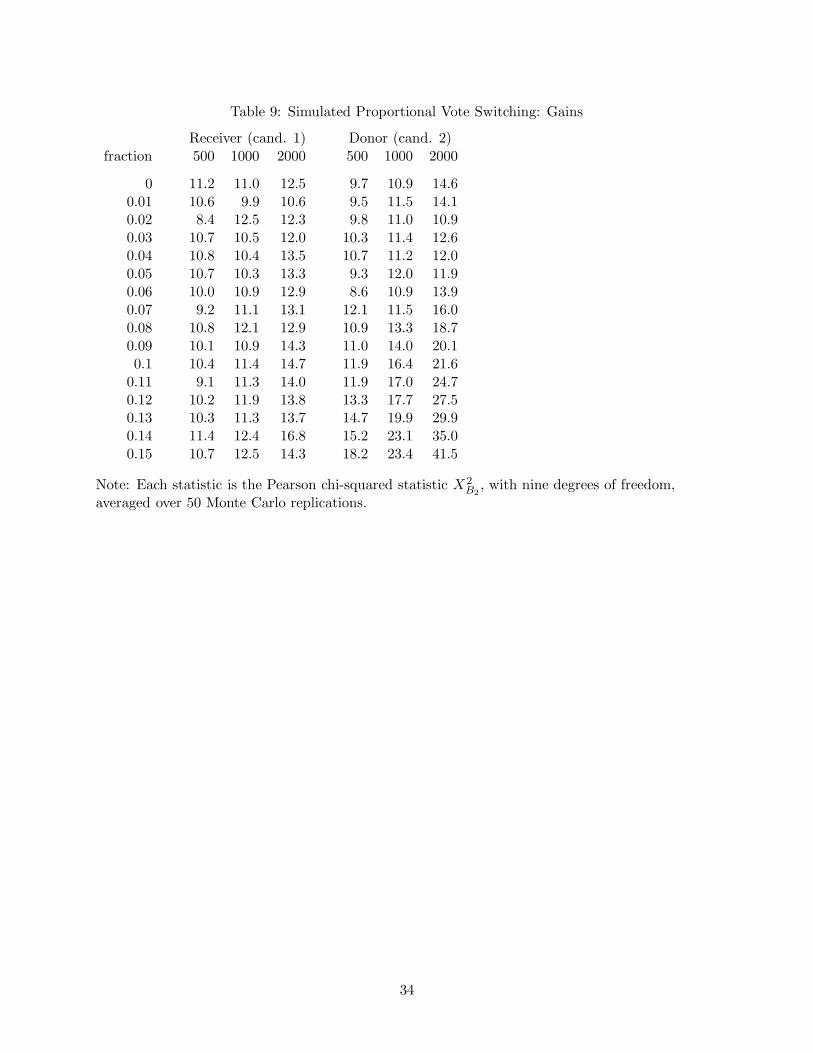
Table 9: Simulated Proportional Vote Switching: Gains
Receiver (cand. 1) Donor (cand. 2)fraction 500 1000 2000 500 1000 2000
0 11.2 11.0 12.5 9.7 10.9 14.60.01 10.6 9.9 10.6 9.5 11.5 14.10.02 8.4 12.5 12.3 9.8 11.0 10.90.03 10.7 10.5 12.0 10.3 11.4 12.60.04 10.8 10.4 13.5 10.7 11.2 12.00.05 10.7 10.3 13.3 9.3 12.0 11.90.06 10.0 10.9 12.9 8.6 10.9 13.90.07 9.2 11.1 13.1 12.1 11.5 16.00.08 10.8 12.1 12.9 10.9 13.3 18.70.09 10.1 10.9 14.3 11.0 14.0 20.10.1 10.4 11.4 14.7 11.9 16.4 21.6
0.11 9.1 11.3 14.0 11.9 17.0 24.70.12 10.2 11.9 13.8 13.3 17.7 27.50.13 10.3 11.3 13.7 14.7 19.9 29.90.14 11.4 12.4 16.8 15.2 23.1 35.00.15 10.7 12.5 14.3 18.2 23.4 41.5
Note: Each statistic is the Pearson chi-squared statistic X 2B2
, with nine degrees of freedom,averaged over 50 Monte Carlo replications.
34

Table 10: Simulated Proportional Vote Switching with Thresholds: Gains
receive votes when above expectationReceiver (cand. 1) Donor (cand. 2)
fraction 500 1000 2000 500 1000 2000
0 10.4 9.6 11.3 9.3 10.9 12.40.01 10.0 11.6 13.0 9.1 10.1 10.30.02 11.2 12.2 14.8 9.0 10.5 11.00.03 11.3 14.4 18.6 8.8 10.1 13.10.04 12.7 16.3 24.4 9.6 10.7 11.60.05 13.6 19.3 30.8 8.6 12.4 12.10.06 17.5 23.4 39.5 9.7 10.5 14.70.07 17.9 27.6 49.4 9.9 12.5 17.20.08 20.8 33.9 60.3 10.9 12.4 17.80.09 26.4 40.7 69.2 10.8 13.1 18.20.1 26.0 40.4 73.9 10.8 14.3 18.0
0.11 27.1 44.6 79.9 10.8 13.7 18.70.12 29.2 44.9 86.6 12.8 14.9 19.00.13 30.1 52.5 92.3 12.0 14.6 19.80.14 31.8 57.5 99.5 12.2 18.3 22.90.15 37.0 64.7 110.2 12.8 17.9 24.7
receive votes when below expectationReceiver (cand. 1) Donor (cand. 2)
fraction 500 1000 2000 500 1000 2000
0 9.6 11.2 9.6 9.8 9.9 12.40.01 9.9 11.2 13.2 10.2 10.8 13.90.02 9.9 11.1 16.3 11.2 11.1 15.80.03 10.4 15.6 21.4 11.2 12.5 17.30.04 13.1 17.8 25.7 11.0 14.0 17.80.05 15.6 20.7 32.7 11.8 14.1 18.80.06 16.0 27.4 39.9 12.2 15.7 22.30.07 18.9 32.0 51.6 12.6 17.5 24.90.08 20.9 39.5 67.1 12.6 20.3 28.60.09 25.7 42.7 74.9 14.8 19.8 33.50.1 26.7 45.9 77.2 16.1 23.1 39.6
0.11 27.4 45.1 86.3 18.9 26.0 42.80.12 29.9 47.6 89.4 18.3 29.7 51.30.13 32.5 52.6 94.5 21.4 35.5 62.80.14 32.8 54.2 110.0 24.7 39.2 72.80.15 36.0 60.0 114.2 27.8 43.1 79.7
Note: Each statistic is the Pearson chi-squared statistic X 2B2
, with nine degrees of freedom,averaged over 50 Monte Carlo replications.
35

Table 11: Simulated “Repeater” Vote Switching: Gains
Receiver (cand. 1) Donor (cand. 2)fraction 500 1000 2000 500 1000 2000
0 10.6 10.6 11.0 10.5 11.3 11.30.01 9.5 10.3 13.0 10.0 11.1 12.40.02 11.5 9.2 12.8 10.5 10.3 13.20.03 9.9 11.5 14.3 10.6 11.4 11.90.04 10.4 10.7 14.6 9.2 11.6 14.10.05 11.3 10.2 13.5 10.8 9.8 14.10.06 11.0 12.6 15.0 9.5 10.8 16.00.07 10.3 12.0 15.1 9.4 11.4 14.50.08 10.5 12.7 17.6 10.6 11.8 17.70.09 9.6 13.2 17.6 11.3 13.4 20.50.1 11.0 13.3 17.9 11.4 13.3 17.1
0.11 11.1 13.1 19.2 11.6 15.7 22.50.12 10.8 15.7 17.8 13.1 17.5 22.00.13 10.5 13.5 19.9 13.8 17.1 26.90.14 11.1 14.0 19.1 14.4 16.8 29.00.15 12.6 14.7 19.7 15.5 19.2 32.1
Note: Each statistic is the Pearson chi-squared statistic X 2B2
, with nine degrees of freedom,averaged over 50 Monte Carlo replications.
36
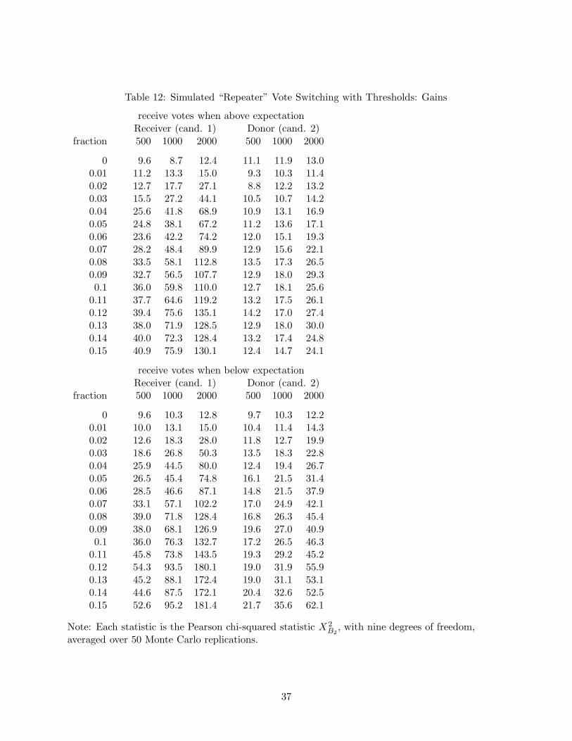
Table 12: Simulated “Repeater” Vote Switching with Thresholds: Gains
receive votes when above expectationReceiver (cand. 1) Donor (cand. 2)
fraction 500 1000 2000 500 1000 2000
0 9.6 8.7 12.4 11.1 11.9 13.00.01 11.2 13.3 15.0 9.3 10.3 11.40.02 12.7 17.7 27.1 8.8 12.2 13.20.03 15.5 27.2 44.1 10.5 10.7 14.20.04 25.6 41.8 68.9 10.9 13.1 16.90.05 24.8 38.1 67.2 11.2 13.6 17.10.06 23.6 42.2 74.2 12.0 15.1 19.30.07 28.2 48.4 89.9 12.9 15.6 22.10.08 33.5 58.1 112.8 13.5 17.3 26.50.09 32.7 56.5 107.7 12.9 18.0 29.30.1 36.0 59.8 110.0 12.7 18.1 25.6
0.11 37.7 64.6 119.2 13.2 17.5 26.10.12 39.4 75.6 135.1 14.2 17.0 27.40.13 38.0 71.9 128.5 12.9 18.0 30.00.14 40.0 72.3 128.4 13.2 17.4 24.80.15 40.9 75.9 130.1 12.4 14.7 24.1
receive votes when below expectationReceiver (cand. 1) Donor (cand. 2)
fraction 500 1000 2000 500 1000 2000
0 9.6 10.3 12.8 9.7 10.3 12.20.01 10.0 13.1 15.0 10.4 11.4 14.30.02 12.6 18.3 28.0 11.8 12.7 19.90.03 18.6 26.8 50.3 13.5 18.3 22.80.04 25.9 44.5 80.0 12.4 19.4 26.70.05 26.5 45.4 74.8 16.1 21.5 31.40.06 28.5 46.6 87.1 14.8 21.5 37.90.07 33.1 57.1 102.2 17.0 24.9 42.10.08 39.0 71.8 128.4 16.8 26.3 45.40.09 38.0 68.1 126.9 19.6 27.0 40.90.1 36.0 76.3 132.7 17.2 26.5 46.3
0.11 45.8 73.8 143.5 19.3 29.2 45.20.12 54.3 93.5 180.1 19.0 31.9 55.90.13 45.2 88.1 172.4 19.0 31.1 53.10.14 44.6 87.5 172.1 20.4 32.6 52.50.15 52.6 95.2 181.4 21.7 35.6 62.1
Note: Each statistic is the Pearson chi-squared statistic X 2B2
, with nine degrees of freedom,averaged over 50 Monte Carlo replications.
37

Table 13: Simulated Proportional Vote Switching: Losses
Donor (cand. 1) Receiver (cand. 2)fraction 500 1000 2000 500 1000 2000
0 10.0 9.6 11.6 9.6 10.1 13.50.01 10.2 10.6 12.0 10.2 10.1 12.60.02 10.3 11.5 12.8 11.2 10.9 11.90.03 9.1 10.7 12.6 9.5 11.4 12.20.04 9.6 10.6 12.2 10.1 11.0 11.60.05 10.6 9.7 12.5 9.4 10.3 12.00.06 9.9 9.5 12.4 10.3 10.7 11.90.07 9.9 10.8 12.9 10.2 10.9 12.60.08 9.0 10.3 11.2 10.5 11.5 14.40.09 9.6 9.4 12.2 9.8 11.3 15.30.1 10.5 10.1 12.2 11.5 11.0 15.5
0.11 9.1 10.1 11.4 9.6 13.5 13.70.12 9.2 9.8 11.4 10.1 11.2 14.80.13 9.1 9.4 12.9 9.3 12.8 15.90.14 9.2 10.1 12.3 10.2 10.9 16.30.15 9.1 10.3 11.1 10.0 11.5 15.6
Note: Each statistic is the Pearson chi-squared statistic X 2B2
, with nine degrees of freedom,averaged over 50 Monte Carlo replications.
38
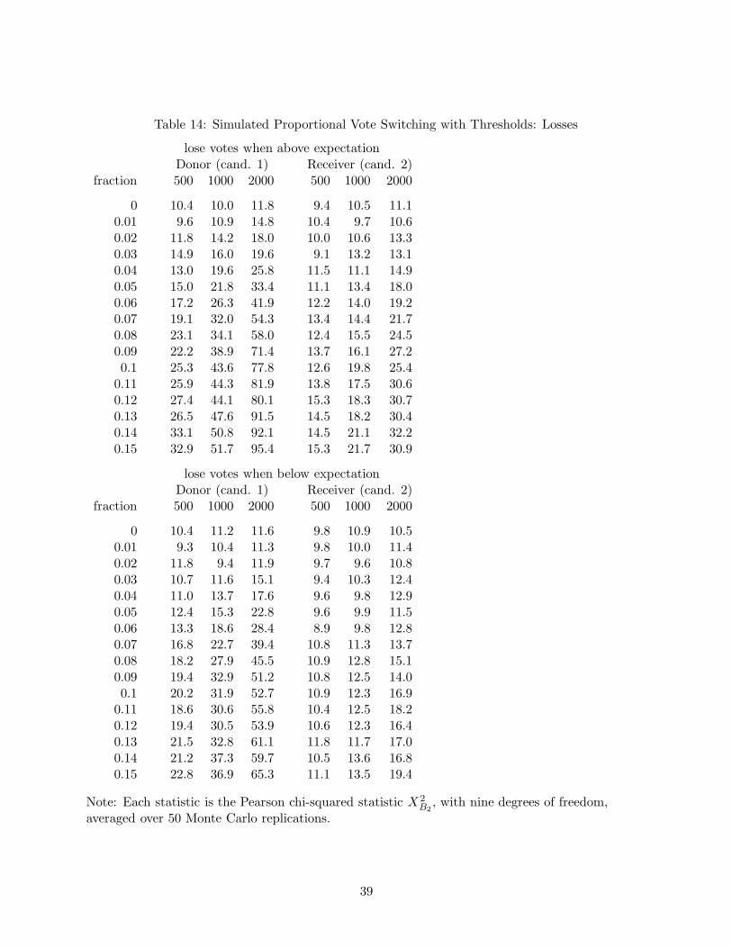
Table 14: Simulated Proportional Vote Switching with Thresholds: Losses
lose votes when above expectationDonor (cand. 1) Receiver (cand. 2)
fraction 500 1000 2000 500 1000 2000
0 10.4 10.0 11.8 9.4 10.5 11.10.01 9.6 10.9 14.8 10.4 9.7 10.60.02 11.8 14.2 18.0 10.0 10.6 13.30.03 14.9 16.0 19.6 9.1 13.2 13.10.04 13.0 19.6 25.8 11.5 11.1 14.90.05 15.0 21.8 33.4 11.1 13.4 18.00.06 17.2 26.3 41.9 12.2 14.0 19.20.07 19.1 32.0 54.3 13.4 14.4 21.70.08 23.1 34.1 58.0 12.4 15.5 24.50.09 22.2 38.9 71.4 13.7 16.1 27.20.1 25.3 43.6 77.8 12.6 19.8 25.4
0.11 25.9 44.3 81.9 13.8 17.5 30.60.12 27.4 44.1 80.1 15.3 18.3 30.70.13 26.5 47.6 91.5 14.5 18.2 30.40.14 33.1 50.8 92.1 14.5 21.1 32.20.15 32.9 51.7 95.4 15.3 21.7 30.9
lose votes when below expectationDonor (cand. 1) Receiver (cand. 2)
fraction 500 1000 2000 500 1000 2000
0 10.4 11.2 11.6 9.8 10.9 10.50.01 9.3 10.4 11.3 9.8 10.0 11.40.02 11.8 9.4 11.9 9.7 9.6 10.80.03 10.7 11.6 15.1 9.4 10.3 12.40.04 11.0 13.7 17.6 9.6 9.8 12.90.05 12.4 15.3 22.8 9.6 9.9 11.50.06 13.3 18.6 28.4 8.9 9.8 12.80.07 16.8 22.7 39.4 10.8 11.3 13.70.08 18.2 27.9 45.5 10.9 12.8 15.10.09 19.4 32.9 51.2 10.8 12.5 14.00.1 20.2 31.9 52.7 10.9 12.3 16.9
0.11 18.6 30.6 55.8 10.4 12.5 18.20.12 19.4 30.5 53.9 10.6 12.3 16.40.13 21.5 32.8 61.1 11.8 11.7 17.00.14 21.2 37.3 59.7 10.5 13.6 16.80.15 22.8 36.9 65.3 11.1 13.5 19.4
Note: Each statistic is the Pearson chi-squared statistic X 2B2
, with nine degrees of freedom,averaged over 50 Monte Carlo replications.
39

Table 15: Simulated “Repeater” Vote Switching: Losses
Donor (cand. 1) Receiver (cand. 2)fraction 500 1000 2000 500 1000 2000
0 10.0 9.6 11.6 9.6 10.1 13.50.01 10.1 10.4 13.1 10.0 10.5 14.20.02 10.4 10.8 12.2 9.4 10.1 12.50.03 10.8 12.5 12.8 9.8 12.4 12.40.04 10.2 10.2 11.9 10.1 11.6 12.20.05 9.4 10.6 12.8 9.6 11.2 13.40.06 10.6 11.5 15.2 10.5 11.6 14.40.07 11.0 11.4 15.2 10.7 11.4 14.60.08 10.5 14.0 17.8 11.3 12.3 16.00.09 10.3 11.3 18.4 10.2 12.2 17.00.1 12.2 13.8 17.5 11.3 12.5 17.8
0.11 13.8 15.1 20.7 11.3 15.5 18.90.12 12.1 17.2 25.3 10.6 14.4 21.50.13 12.7 17.5 26.9 12.3 14.5 21.90.14 15.3 19.1 29.4 11.3 14.3 19.00.15 14.6 18.6 32.1 12.4 14.5 21.4
Note: Each statistic is the Pearson chi-squared statistic X 2B2
, with nine degrees of freedom,averaged over 50 Monte Carlo replications.
40

Table 16: Simulated “Repeater” Vote Switching with Thresholds: Losses
lose votes when above expectationDonor (cand. 1) Receiver (cand. 2)
fraction 500 1000 2000 500 1000 2000
0 10.4 10.0 11.8 9.4 10.5 11.10.01 10.8 12.9 19.6 10.0 11.2 12.60.02 15.6 21.5 32.2 11.0 13.0 16.40.03 22.1 29.5 47.1 11.6 16.9 21.10.04 24.6 42.5 71.9 15.2 20.8 29.10.05 26.0 41.7 75.1 14.6 20.5 34.30.06 26.4 49.7 87.4 17.7 23.0 36.10.07 33.7 55.6 108.4 17.9 26.7 45.90.08 37.3 64.4 127.2 18.1 30.1 48.80.09 35.9 58.7 120.6 21.5 32.6 57.40.1 35.9 61.4 115.7 20.7 37.6 60.8
0.11 34.7 63.7 117.3 24.8 41.6 70.90.12 41.8 71.6 143.0 27.4 41.0 75.00.13 39.5 65.7 131.3 25.6 41.7 78.70.14 41.9 70.9 134.8 25.9 45.0 85.60.15 42.6 67.3 130.3 31.5 49.2 86.1
lose votes when below expectationDonor (cand. 1) Receiver (cand. 2)
fraction 500 1000 2000 500 1000 2000
0 10.4 11.2 11.6 9.8 10.9 10.50.01 9.8 10.7 14.3 10.1 9.6 11.10.02 11.7 14.5 21.1 11.0 9.5 10.90.03 16.4 23.5 33.9 10.7 10.5 13.90.04 21.4 37.1 60.7 10.9 13.2 18.50.05 20.0 33.1 58.2 11.2 13.7 18.30.06 22.6 35.7 63.7 11.3 13.0 20.10.07 26.1 39.7 73.5 13.8 15.6 23.00.08 29.8 50.3 96.3 13.4 19.2 27.60.09 26.1 50.4 85.3 14.4 19.8 24.70.1 28.1 45.5 85.3 13.0 20.0 30.6
0.11 26.9 39.7 74.8 13.5 20.5 33.60.12 30.2 49.4 94.6 13.9 21.8 37.60.13 29.6 48.9 91.4 14.8 22.6 38.60.14 27.4 46.0 87.4 14.6 23.2 34.60.15 24.0 43.4 75.9 16.0 24.3 38.2
Note: Each statistic is the Pearson chi-squared statistic X 2B2
, with nine degrees of freedom,averaged over 50 Monte Carlo replications.
41

Table 17: Precinct, Machine and Ballot Statistics
Election Day Broward Miami-Dade PascoPrecincts 775 757 152Machines 5,306 5,323 1,338Precinct-machines 10,614 14,128 2,676Ballots 431,488 435,902 127,526
Early Voting Broward Miami-Dade PascoSites 20 14 3Styles 150 100 16Site-days 110 — 4Style-site-days — 4,429 —Machines 190 726 36Site-day-machines 380 — 72S-s-d-machines — 24,374 —Ballots 176,743 242,344 29,584
42

Table 18: Miami-Dade Early Voting Second-digit Benford’s Law Tests
site- site-style-style-days machines day-machines
(n = 5, 186) (n = 727) (n = 33, 126)item Benf. equal Benf. equal Benf. equal
Bush 10.1 44.9 23.5 20.9 130.3 391.4Kerry 17.3 60.4 61.7 12.1 115.5 387.3Martinez 14.8 48.6 32.6 17.3 107.6 357.9Castor 9.1 42.1 43.3 18.6 93.0 336.2Am. 1 Yes 14.1 59.9 69.6 9.8 119.7 415.4Am. 1 No 8.7 44.1 64.8 9.8 86.3 295.7Am. 2 Yes 17.7 65.4 58.3 2.6 83.4 334.7Am. 2 No 20.2 71.1 41.9 16.9 92.0 292.8Am. 3 Yes 8.2 41.4 90.8 7.6 122.7 394.8Am. 3 No 15.3 56.7 66.1 7.8 104.8 342.1Am. 4 Yes 7.7 40.6 47.1 11.0 87.3 338.0Am. 4 No 14.4 60.7 83.6 5.3 108.9 351.4Am. 5 Yes 21.9 78.3 69.2 4.6 58.4 307.5Am. 5 No 11.0 44.8 5.7 71.6 84.4 237.8Am. 6 Yes 12.9 56.9 55.3 11.0 105.2 368.5Am. 6 No 9.0 37.8 44.4 9.6 126.6 374.1Am. 7 Yes 24.6 85.0 47.8 14.9 134.2 468.3Am. 7 No 12.0 33.9 77.4 236.4 64.5 192.7Am. 8 Yes 13.9 61.7 68.9 2.4 96.3 377.7Am. 8 No 6.7 28.9 63.5 15.5 79.2 261.2
Note: Each statistic is the Pearson chi-squared statistic, with nine degrees of freedom.
43

Table 19: Broward Second-digit Benford’s Law Tests
Election Day Early Votingprecincts machines styles machines(n = 775) (n = 5, 307) (n = 150) (n = 190)
item Benf. equal Benf. equal Benf. equal Benf. equal
Bush 9.6 6.6 23.4 25.6 9.1 12.2 8.4 9.5Kerry 21.2 12.4 79.7 6.5 21.4 24.8 10.5 17.6Martinez 10.7 8.3 28.2 20.1 6.6 9.8 5.2 8.6Castor 13.6 5.9 69.7 11.4 9.2 6.7 11.4 17.5Am. 1 Yes 24.1 16.3 31.2 8.5 10.1 12.2 14.9 10.0Am. 1 No 17.1 18.1 60.3 8.4 7.0 3.7 7.0 7.2Am. 2 Yes 12.2 7.3 47.5 21.7 13.6 11.7 19.4 16.8Am. 2 No 11.6 22.4 47.6 18.8 8.7 9.8 4.8 3.9Am. 3 Yes 7.4 6.4 65.8 9.1 8.1 11.8 11.0 14.9Am. 3 No 24.9 6.7 40.5 11.7 11.9 17.7 5.4 4.6Am. 4 Yes 9.8 7.7 61.3 5.8 14.4 15.5 14.2 22.7Am. 4 No 8.6 16.2 55.8 10.1 4.7 10.1 10.5 8.2Am. 5 Yes 7.9 8.8 76.9 17.5 13.8 13.0 15.6 20.9Am. 5 No 7.4 20.6 24.8 113.4 5.2 4.1 9.7 8.4Am. 6 Yes 19.4 9.9 84.9 10.3 4.4 4.4 11.9 16.8Am. 6 No 6.2 10.9 43.7 5.6 7.8 10.1 16.6 16.4Am. 7 Yes 13.1 16.7 72.1 6.6 5.0 8.6 44.0 64.2Am. 7 No 14.3 44.3 157.7 346.9 8.9 9.6 5.7 8.7Am. 8 Yes 7.1 3.8 74.6 6.3 4.3 6.2 27.9 42.9Am. 8 No 13.9 26.1 15.9 21.7 6.7 7.3 4.0 7.7
Note: Each statistic is the Pearson chi-squared statistic, with nine degrees of freedom. InBroward, on election day each machine recorded votes for only one precinct. In the early votingdata the number of votes on each style-machine combination was too small (mean = 16.7, median= 2) to support analysis for those combinations.
44

Table 20: Pasco Second-digit Benford’s Law Tests
Early VotingElection Day machine-
precincts machines precincts(n = 152) (n = 1, 338) (n = 372)
item Benf. equal Benf. equal Benf. equal
Bush 6.9 5.6 16.4 16.2 14.6 23.8Kerry 4.0 3.5 22.9 21.7 19.0 25.2Martinez 6.5 3.7 30.6 6.4 13.4 24.3Castor 11.2 10.5 40.5 7.7 14.7 20.7Am. 1 Yes 9.0 10.4 24.1 11.3 5.4 10.5Am. 1 No 7.0 5.1 9.8 5.0 18.6 28.3Am. 2 Yes 5.4 4.8 28.6 10.3 9.6 16.2Am. 2 No 8.6 12.7 15.8 1.9 10.4 17.7Am. 3 Yes 10.4 9.3 34.6 11.0 12.5 18.6Am. 3 No 8.5 4.4 10.1 16.2 13.1 19.2Am. 4 Yes 6.0 8.4 20.7 2.8 8.6 14.7Am. 4 No 8.6 5.2 19.8 9.3 21.5 33.4Am. 5 Yes 3.6 9.4 16.6 8.2 11.9 20.9Am. 5 No 3.8 6.4 10.2 19.1 10.3 17.2Am. 6 Yes 12.8 15.5 33.5 7.7 10.5 18.7Am. 6 No 4.4 4.7 20.1 10.0 14.4 16.4Am. 7 Yes 29.5 43.3 20.5 18.3 14.1 22.3Am. 7 No 5.1 7.2 19.9 10.7 5.2 6.9Am. 8 Yes 8.0 13.8 16.5 7.7 6.3 8.6Am. 8 No 8.0 14.6 29.9 6.6 11.1 18.1
Note: Each statistic is the Pearson chi-squared statistic, with nine degrees of freedom. In Pasco,on election day each machine recorded votes for only one precinct. In Pasco there were only 16early voting “precincts,” too few to support analysis for those units.
45

Table 21: Mexico 2006 Presidential Vote Second-digit Benford’s Law Tests: Secciones
Seccion-level 2BL test statistics
State n PAN PRD PRI NA ASDC
All 64,679 48.1 25.3 109.0 1254.8 16.6Aguascalientes 593 6.6 14.2 6.0 18.9 8.3Baja California 1,525 12.0 34.9 13.4 49.5 20.4Baja California Sur 351 6.3 17.7 15.6 13.7 4.0Campeche 491 8.3 19.2 7.7 11.8 8.6Coahuila 1,938 8.3 22.5 4.7 23.2 15.8Colima 2,918 9.9 11.7 25.1 131.6 43.6Chiapas 1,537 16.1 15.3 5.6 44.6 12.8Chihuahua 338 15.7 10.6 10.1 11.4 6.9Distrito Federal 5,560 10.9 26.9 42.6 178.9 61.6Durango 1,382 5.1 11.1 9.8 51.1 16.3Guanajuato 3,043 13.7 7.2 25.4 117.9 6.6Guerrero 2,767 14.4 8.8 28.0 65.8 11.9Hidalgo 1,712 5.8 5.4 19.3 50.8 4.9Jalisco 3,363 18.1 24.0 16.3 81.6 12.3Mexico 6,193 51.4 49.8 15.0 238.4 18.0Michoacan 2,687 14.0 5.5 16.8 49.7 25.0Morelos 912 14.1 17.3 8.8 17.4 11.5Nayarit 879 5.6 7.2 8.8 23.7 10.6Nuevo Leon 2,148 8.6 11.8 9.3 7.9 7.3Oaxaca 2,456 16.3 9.4 14.4 38.9 19.8Puebla 2,566 18.5 20.9 16.7 104.3 10.7Queretaro 761 16.8 12.6 6.3 25.5 10.1Quintana Roo 445 11.6 6.7 5.9 8.8 7.5San Luis Potosi 1,797 9.7 9.6 24.9 43.2 8.1Sinaloa 3,771 39.1 25.9 17.1 36.4 87.9Sonora 1,361 23.1 3.9 20.3 45.5 8.5Tabasco 1,139 7.3 16.3 13.6 6.4 29.0Tamaulipas 1,743 10.7 9.3 13.8 56.8 12.7Tlaxcala 611 8.4 13.5 11.5 23.5 12.6Veracruz 4,736 14.0 9.5 19.1 75.2 28.7Yucatan 1,083 20.9 31.0 6.6 46.5 7.5Zacatecas 1,873 10.2 12.9 14.5 35.3 38.5
Note: Each statistic is the Pearson chi-squared statistic, with nine degrees of freedom. The valuesin the n column show the total number of secciones in each state (or, for “All,” across the wholecountry), not the number of vote counts that have two digits. That number varies among theparties.
46

Table 22: Mexico 2006 Presidential Vote Second-digit Benford’s Law Tests: Casillas
Casilla-level 2BL test statistics
State n PAN PRD PRI NA ASDC
All 130,768 660.7 104.7 217.7 1712.2 2751.1Aguascalientes 1,229 14.8 13.6 17.3 46.4 29.1Baja California 3,550 174.5 44.3 24.9 92.5 223.5Baja California Sur 664 41.9 42.3 3.0 6.4 23.3Campeche 929 50.7 50.0 46.2 6.4 54.9Coahuila 4,784 15.2 19.5 24.8 23.4 118.1Colima 4,742 49.7 33.7 57.1 150.4 374.6Chiapas 3,094 68.9 25.9 30.7 16.5 167.4Chihuahua 762 9.5 37.6 85.2 14.7 53.3Distrito Federal 12,235 105.9 71.4 142.7 17.3 134.8Durango 2,236 8.5 27.1 17.5 58.1 141.4Guanajuato 6,136 10.3 19.5 9.2 86.0 267.3Guerrero 4,478 17.7 49.4 14.6 38.9 155.8Hidalgo 3,055 41.8 62.0 31.1 164.4 70.9Jalisco 8,110 98.8 41.5 272.5 276.9 160.6Mexico 15,553 144.1 70.2 37.7 460.8 113.5Michoacan 5,427 23.0 239.6 20.9 13.1 249.1Morelos 2,067 36.7 40.0 26.1 56.2 89.7Nayarit 1,395 7.1 38.8 64.2 41.4 47.7Nuevo Leon 5,066 28.8 32.1 182.7 177.2 286.1Oaxaca 4,479 21.3 6.7 46.6 16.0 123.4Puebla 6,037 56.5 327.1 22.3 74.5 112.2Queretaro 1,807 25.6 71.9 17.7 37.6 66.4Quintana Roo 1,154 27.9 31.1 12.8 11.5 64.4San Luis Potosi 3,094 10.2 15.0 8.7 50.5 42.1Sinaloa 4,300 84.1 35.7 11.9 10.9 136.7Sonora 3,011 50.2 27.8 8.5 21.4 222.9Tabasco 2,408 80.4 25.9 69.9 8.9 30.2Tamaulipas 3,971 106.6 62.2 57.5 68.6 323.6Tlaxcala 1,255 71.6 31.4 26.8 18.2 79.5Veracruz 9,185 169.9 100.4 27.2 31.1 302.5Yucatan 2,157 24.4 11.4 71.7 20.8 45.6Zacatecas 2,398 29.0 43.8 13.6 55.8 62.3
Note: Each statistic is the Pearson chi-squared statistic, with nine degrees of freedom. The valuesin the n column show the total number of casillas in each state (or, for “All,” across the wholecountry), not the number of vote counts that have two digits. That number varies among theparties.
47

8 10 12 14 16 18
24
68
1012
14
precinct 109
times
mac
hine
s
aaaaaaaaaaaaaaaaaaa aaaaa aaaaa aaa aa a aa aaa a aaa aaaaaa a
bbbbbbbbbbbbbbbbbbbbbbbbbbbbbbbbbbbb bbbbbbbbbbb b bbbb bbbbbbbbbbbbbbbbb bbbbbbbbbbbbb
ccccccccccccccccccccccccccccc ccccc c ccc ccccc ccc c c c cc ccc ccccccc c c
dddddddddddddddddddddddd ddddd ddddd d d d d d d dd dd ddd
eeeeeeeeeeeeeeeeeeeeeeee e
ffffffffffffffffffffff ffff fff fff f ffff fff fff ff fffff f f fff f f fff ff fff ff f f ff fff f ff f f f
ggggggggggggggggggggggggggggggggg gggggg ggggggggggggg ggggggggggggggggg ggg
hhhhhhhhhhhhhhhhhhh hhhh hhhh hhhhhhhhhhhhh hhhhh h hh hhhhh hhhh hhhh
iiiii iii iiiiiiii ii iii ii i iii i i i ii i i ii ii ii ii i i i i i i i i i ii i i i i ii ii i i
jjjjjjjj jjjjjjj jjjj j j j jj jjj j jjj jj j j jj jj j j jj jj j j jj j j j j j j j j j j j j j j j
kkkkkkkkkkkkkkkk kkk k kkkkkkkkkk k k k kk k
lll l llllllll llll l ll l l ll l lll l l lll l ll l l l l l l l l lll l l l l l
mmmmmmmmmmmmmmmmmmmmmmmmmmm mmmmmmmmmm mmmmmmmmmmmmmmmmmmmmmmmmmmm mmm
nnnnnnnnnnnnnnnnnnnn nn nnnn nnnnnnn nn n n n n n n nnn nn n
8 10 12 14 16 18 20
24
68
precinct 233
times
mac
hine
s
aaaaaaaaaaaaaaaaaaaaaaaaaaaaaaaaaaaaaaaaaaaaaaaaaaaaaaaaaaaaaaaaaaaaaaaaaaaaaaaaaaaaaaaaaaaaaaaaaaaaaaaaaaaaaa
bbbbbbbbbbbbbbbbbbbbb bbbbbbbbbbbbbbbbbbbbbbbbbbbbbbbbbbbbbbbbbbbbbbbbbbbbbbbbbbbbbbbbbbbbbbbbbbbbbbbbb bbb
ccccccc
ddddddddddddddddddddddddddddddddddddddddddddddddddddddddddddddddddddddddddddddddddddddddddddddddddddddddd
eeeeeeeeeeeeeeeeeeeeeeeeeeeeeeeeee eeeeeeeeeeeeeeeeeeeeeeeeeeeeeeeeeeeeeeeeeeeeeeeeeeeeeeeeeeeeeeee
f ffffff f ffffff f fff fffffffffffffffffffff fff f f ff
ggggggggggggg gggggggggggggggggggggggggggggggggggggggggggggggggggggggggggg ggggggggggggggggggggggg
hhhh hhhhhhhhhhhhhhhhhhhhhhhhhhhhhhhhhhhhhh hhhhhhhhhhhhhhhhhh hhhhhhhhhhhhhhhhhhhhhhhhhh
iiiii iiiii i iiii iiiiii iii iiii iii i i iiiiiiii iiii i ii iii iiii ii iiiiii iii i i iii i iiiiii iii ii ii iiii iii i i i i iiii
8 10 12 14 16 18 20
510
15
precinct 322
times
mac
hine
s
aaaaaaaaaaaaaaaaaaaaa aaaaaaaaaaaaaaaaaaaaaaaaaaaaaaaaaaaaaaaaaa aaaaaaaaaaaaaaaaaaaaaaaaaaaaaabbbbbbbbbbbbbbbbbb
cccccccccccccccccccccc cccccccccccccc ccccccccccccccccccccccccccc cccddddddddd dddddddddd dddddddd ddddddddddddddddddddddddddddddddddddddddddddddddddddddddd
eeeeeeeeeeeeeeeeeeeeeeeeeeeeeeeeeeeeeeeeeeeeeeeeee eeeeeeeeeeeeeeeeeeeeeeeeee eeeeeeeeeeeeef fff ffffffff ffffffff fffff fff f fffffffffffff f f fffffffffffff f ff ffffffff ffffff ffffff ff ff fff ffffff
gggggggggggggggggggggg ggggggggggggggggggggggggggggggggggggggggggggggggggggggggggggggggggggggghhhhhhhhhhhhhhhhhhhhhh hhhhhhhhhhhhhhhhhhhhhhhhhhhhhhhhhhhhhhhhhhhhhhhhhhhhhhhhhhhhhhhhhhi i i i ii i ii i iiiiii ii i i i iii i iiiiiii i i iiiiii iii iiii ii ii i ii iiii i iiiii iiiiii ii i i i ii i i iiii iii
jjjj j j jj jjjj j jjj jj j jj jj jjj jj jjjj jjj jjj jjjjjjjjjjjj jjj j j j jjj j jj j j j jjjj j jjjjj j j j jj jjjjj j j j j jjjj j jkkkkkkkkkkkkkkkkkkkkkkk kk kkkk kkkkkkkkk kkkkk kkkkkkkkkkkkkkk kkkkkkkkkkkkkkkkkkkkkkkkkkkkkkkkkkk
lll ll l l ll lllll l ll lll ll l ll l ll ll llll ll ll ll l l lll lll l l l l l l lll llllll ll l ll l llll l lll l l ll l lllll ll
mmmmmmmmmmmmmmmmmmmmmmmmmmmmmmmmmmmmmmmmmmmmmmmmmmmmmmmmmmmmmmmmmmmmmmmmmmmmmmmmmmmmmmmmmmmnnnnnnnnnnnnnnnnnnn nnnnnnnnnnnnnnnn nnnnnnnnnnnnnnnnnnnnnnnnnnnnnnnnnnnnnnnnn nnnnnnnnnnnnn
ooooooooo ooooooooooooooooooooooooooooooooooooooooooooooooooooooooooooooooooooooooooooooooooo
ppppppppp ppppp ppppppppppppppppppppppppppppppppppppppppppppppppppppppppppppppppppppp
8 10 12 14 16 18 20
510
15
precinct 326
times
mac
hine
s
aaaaaaaaaaaaaaaaaaaaaaaaaaaaaaaaaaaaaaaaaaaaaaaaaaaaa aaaaaaaaaa aaaaa aaaaaaaaaaaaaaaaabbbbbbbbbbbbbbbbbbbbbb bbbbbbbbbbbbbbbbbbbbbbbbbbbbbbbbbbbbbbbbbbbbbbbbbbbbbbbbbbbbbbbbccccccccccccccccccccccccccccccccccccccc cccccccccccccccccccccccccccc ccccccccccccccccccccccccccddddddddddddddddddddddddddddddddddddddddd dddddddddddddddddddddddddddddd ddddddddddddddeeeeeeee e eeeeeeeeeeee eeeeeeeeeeeeeeeeeeee eeeeeeeeeee eeeeeeeeeeeeeeeeeeeeeeeeeeeeeeeeeeee
fffffffffffffffffffff ffffffffffff fff ff ff fff fff fff f fffff ffffff ff ff ffffffffff fff fff fffff ffff ff f f
ggggggggggggggggggggggggggggggggggggggggggg ggggghhhhhhhhhhhhhhhhhhhhhhhhhhhhhhhhhhhhhhhhhhhhhhhhhhhhhhhhhhhhhhhhhhhhhhhhhhhhhhhhhhhhhhhhh hi iiii iiii iiii i i i iiiiiii iiiiii iii iiii i ii i i i ii i i ii i iii ii ii i i i iii ii ii i i i iiii ii i iii i i i ii ii
j j jjjjjjjjj jj jj j j jjj jjj j jjj j j j j j j j j jjjj j j jj jjj j jjjjjjjj j j jjjjj j jjj jj jjjjjj j j jjjj jj jjj j jkkkkkkkkkkkkkkk kkkkkkkkkkkkkkkk kk kkkkkkkkkkkkkkkkkkkkk kkkkkkkkkkkk kkkkkkkkkkkkkk kllll llllllllllll ll l l ll lllll l l l ll ll l llllll lllllll lll ll lll l ll l l ll l ll ll lllll ll lll l llllll l lll ll l
mmmmmmmmmmmmmmmmmmmmmmmmmmmmmmmmmmmmmmmmmmmmmmmmmmnnnnnnnnnnnnnnnnnnnnnnnnnnnnnnnnnnnnnnnnnnnnnnnnnnnnnnnnnnnnnnnnnnnnnnnnnnnnnnnnnnnnnnnnnn
ooooooooooo oooooooooooooooooooooooooooooooooooooooooooooooooooooooooooooooooooooooooooooooooooooooop ppp p p p p p pp ppppppppppqqqqqqqqqqqq qqqqqqqqqqqqqqqqqqqqqqqqqqqqqqqqqqqqqqqqqqqqqqqqqqqqqqqqqqqqqqqqqqqqqqqqqqqqqqq
Figure 1: Times (Resolved to the Second and Shown on a 24-Hour Clock) When Votes Were Caston Machines in Selected Precincts on Election Day, Miami-Dade County
48