Elasto-plastic concrete beam analysis by 1-dimensional ... · purely elastic and implementing...
117
A ALBORG U NIVERSITY MASTER ’ S T HESIS Elasto-plastic concrete beam analysis by 1-dimensional Finite Element Method Authors: Niels F. Overgaard Martin B. Andreasen Supervisors: Johan Clausen Lars V. Andersen A thesis submitted in fulfilment of the requirements for the degree of M.Sc. in Engineering in the Department of Civil Engineering June 6, 2016
Transcript of Elasto-plastic concrete beam analysis by 1-dimensional ... · purely elastic and implementing...
AALBORG UNIVERSITY
MASTER’S THESIS
Elasto-plastic concrete beamanalysis by 1-dimensional Finite
Element Method
Authors:
Niels F. Overgaard
Martin B. Andreasen
Supervisors:
Johan Clausen
Lars V. Andersen
A thesis submitted in fulfilment of the requirements
for the degree of M.Sc. in Engineering
in the
Department of Civil Engineering
June 6, 2016

III
School of Engineering and ScienceStudy board of Civil EngineeringFibigerstræde 109220 Aalborg ØstPhone: 99 40 84 84http://www.byggeri.aau.dk
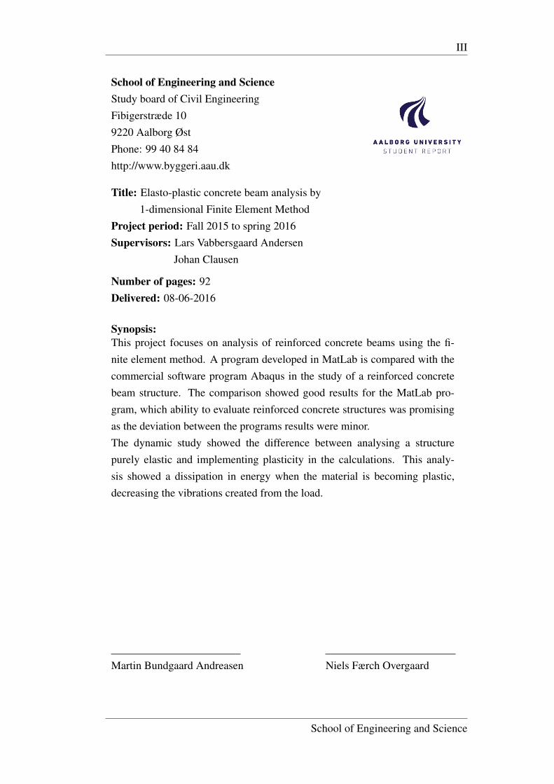
Title: Elasto-plastic concrete beam analysis by1-dimensional Finite Element Method
Project period: Fall 2015 to spring 2016Supervisors: Lars Vabbersgaard Andersen
Johan Clausen
Number of pages: 92Delivered: 08-06-2016
Synopsis:This project focuses on analysis of reinforced concrete beams using the fi-nite element method. A program developed in MatLab is compared with thecommercial software program Abaqus in the study of a reinforced concretebeam structure. The comparison showed good results for the MatLab pro-gram, which ability to evaluate reinforced concrete structures was promisingas the deviation between the programs results were minor.The dynamic study showed the difference between analysing a structurepurely elastic and implementing plasticity in the calculations. This analy-sis showed a dissipation in energy when the material is becoming plastic,decreasing the vibrations created from the load.
Martin Bundgaard Andreasen Niels Færch Overgaard
School of Engineering and Science

V
PrefaceThis report presents the master thesis from the master program in Structural and
Civil Engineering at Aalborg University. The report is written by Niels FærchOvergaard and Martin Bundgaard Andreasen. The subject is "Elasto-plastic con-
crete beam analysis by 1-dimensional Finite Element Method". The project wasdone over two semesters during the fall semester 2015 and the spring semester2016 and delivered on 10.06.2016. The project was supervised by Johan Clausenand Lars Andersen.
Reading guidelinesThe bibliography is a collection of the references used throughout the report andcan be found in the back of the report. Here, all sources are presented with theneeded information. Sources are presented via the Harvard Method. A referenceis given as: [Author, Year].
For each chapter in the main report, tables, figures and equations are given ref-erence numbers corresponding to the current chapter. For better understanding ofthe reader, commentary text is added to each table and figure.
Appendices, for a better understanding of parts of the main report, are found inthe back of the report. Further, a digital appendix is placed on a CD, attached tothe report. The digital appendix consist of MatLab scripts and the report as a PDFversion.
School of Engineering and Science

VII
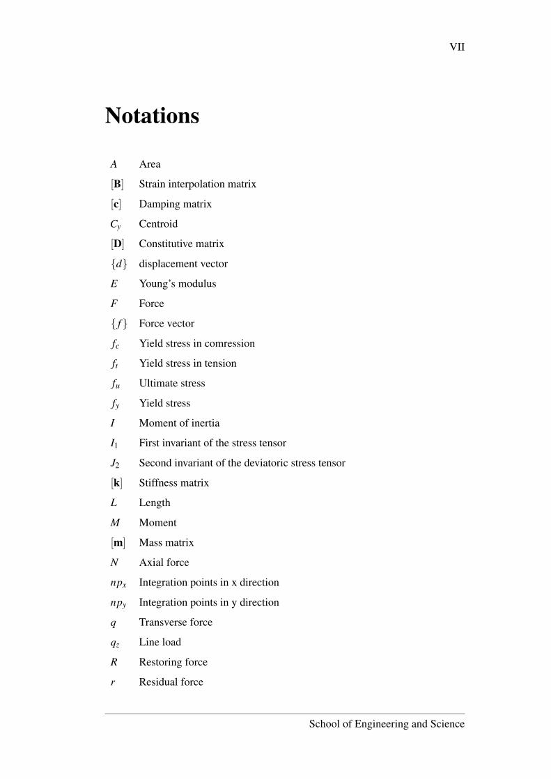
Notations
A Area
[B] Strain interpolation matrix
[c] Damping matrix
Cy Centroid
[D] Constitutive matrix
{d} displacement vector
E Young’s modulus
F Force
{ f} Force vector
fc Yield stress in comression
ft Yield stress in tension
fu Ultimate stress
fy Yield stress
I Moment of inertia
I1 First invariant of the stress tensor
J2 Second invariant of the deviatoric stress tensor
[k] Stiffness matrix
L Length
M Moment
[m] Mass matrix
N Axial force
npx Integration points in x direction
npy Integration points in y direction
q Transverse force
qz Line load
R Restoring force
r Residual force
School of Engineering and Science
VIII
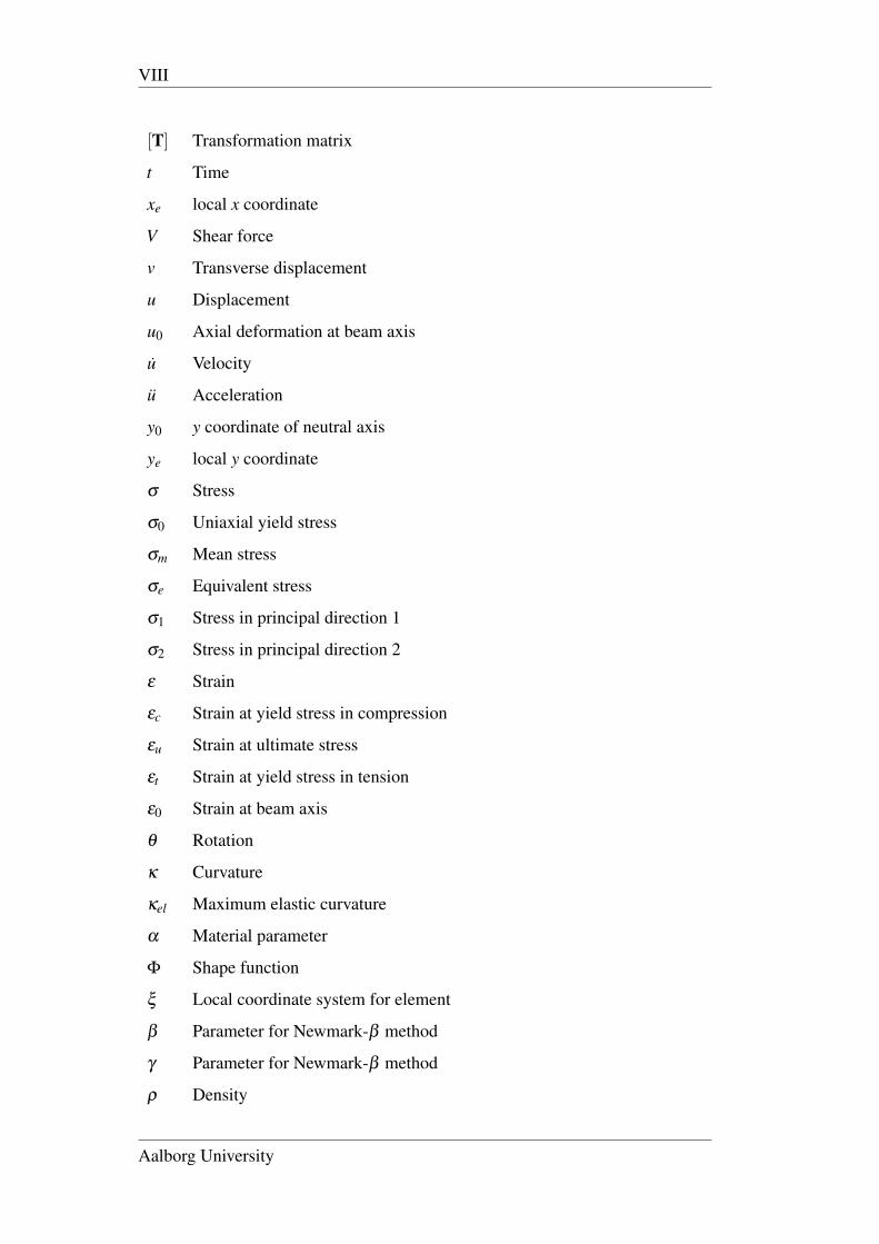
[T] Transformation matrix
t Time
xe local x coordinate
V Shear force
v Transverse displacement
u Displacement
u0 Axial deformation at beam axis
u Velocity
u Acceleration
y0 y coordinate of neutral axis
ye local y coordinate
σ Stress
σ0 Uniaxial yield stress
σm Mean stress
σe Equivalent stress
σ1 Stress in principal direction 1
σ2 Stress in principal direction 2
ε Strain
εc Strain at yield stress in compression
εu Strain at ultimate stress
εt Strain at yield stress in tension
ε0 Strain at beam axis
θ Rotation
κ Curvature
κel Maximum elastic curvature
α Material parameter
Φ Shape function
ξ Local coordinate system for element
β Parameter for Newmark-β method
γ Parameter for Newmark-β method
ρ Density
Aalborg University

IX
ν Poisson’s ratio
School of Engineering and Science

XI
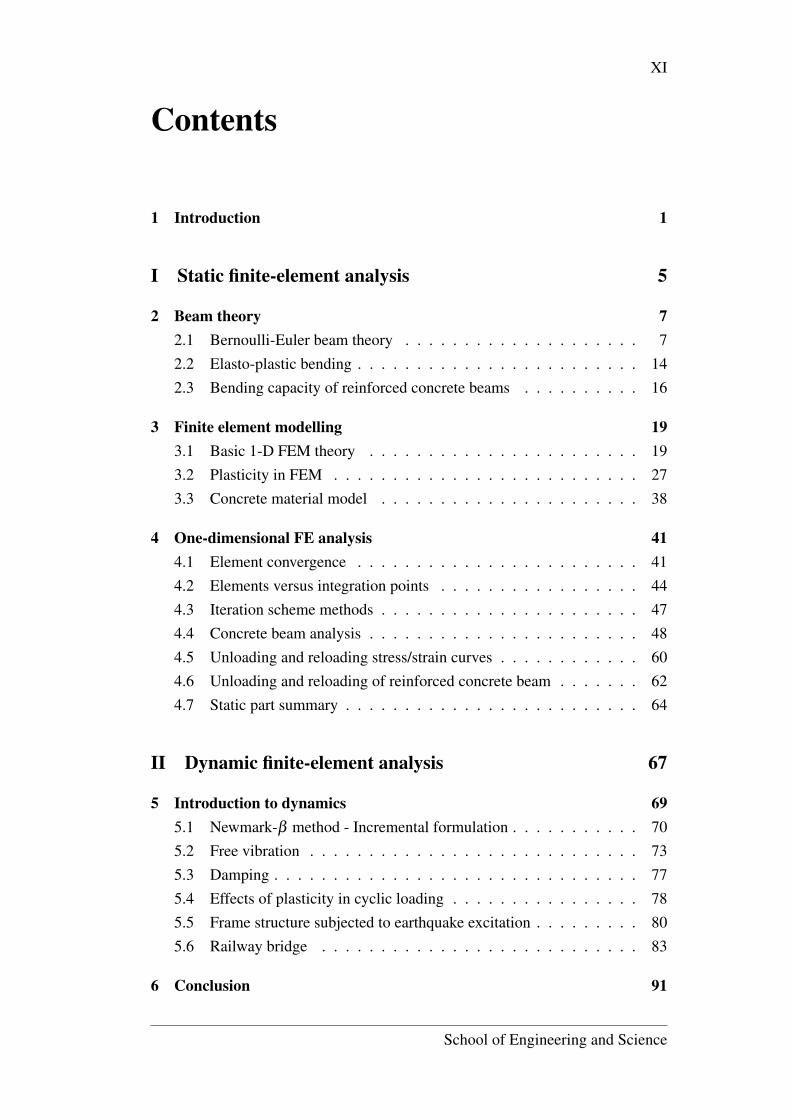
Contents
1 Introduction 1
I Static finite-element analysis 5
2 Beam theory 72.1 Bernoulli-Euler beam theory . . . . . . . . . . . . . . . . . . . . 72.2 Elasto-plastic bending . . . . . . . . . . . . . . . . . . . . . . . . 142.3 Bending capacity of reinforced concrete beams . . . . . . . . . . 16
3 Finite element modelling 193.1 Basic 1-D FEM theory . . . . . . . . . . . . . . . . . . . . . . . 193.2 Plasticity in FEM . . . . . . . . . . . . . . . . . . . . . . . . . . 273.3 Concrete material model . . . . . . . . . . . . . . . . . . . . . . 38
4 One-dimensional FE analysis 414.1 Element convergence . . . . . . . . . . . . . . . . . . . . . . . . 414.2 Elements versus integration points . . . . . . . . . . . . . . . . . 444.3 Iteration scheme methods . . . . . . . . . . . . . . . . . . . . . . 474.4 Concrete beam analysis . . . . . . . . . . . . . . . . . . . . . . . 484.5 Unloading and reloading stress/strain curves . . . . . . . . . . . . 604.6 Unloading and reloading of reinforced concrete beam . . . . . . . 624.7 Static part summary . . . . . . . . . . . . . . . . . . . . . . . . . 64
II Dynamic finite-element analysis 67
5 Introduction to dynamics 695.1 Newmark-β method - Incremental formulation . . . . . . . . . . . 705.2 Free vibration . . . . . . . . . . . . . . . . . . . . . . . . . . . . 735.3 Damping . . . . . . . . . . . . . . . . . . . . . . . . . . . . . . . 775.4 Effects of plasticity in cyclic loading . . . . . . . . . . . . . . . . 785.5 Frame structure subjected to earthquake excitation . . . . . . . . . 805.6 Railway bridge . . . . . . . . . . . . . . . . . . . . . . . . . . . 83
6 Conclusion 91
School of Engineering and Science
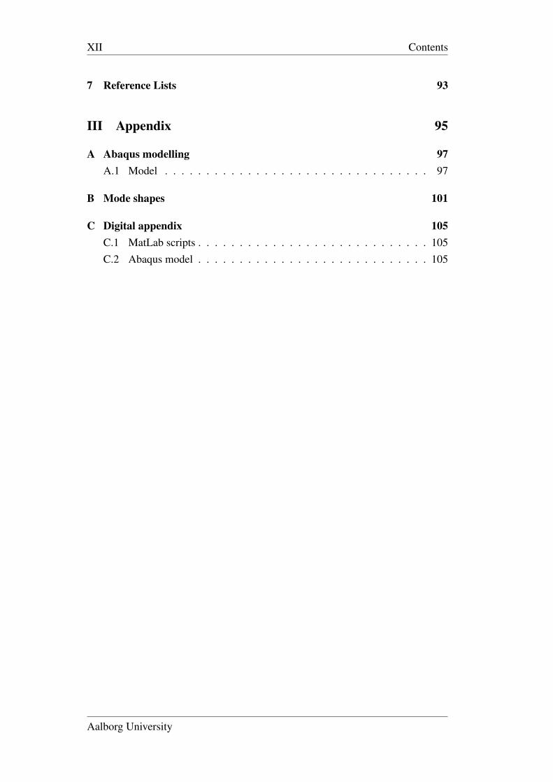
XII Contents
7 Reference Lists 93
III Appendix 95
A Abaqus modelling 97A.1 Model . . . . . . . . . . . . . . . . . . . . . . . . . . . . . . . . 97
B Mode shapes 101
C Digital appendix 105C.1 MatLab scripts . . . . . . . . . . . . . . . . . . . . . . . . . . . . 105C.2 Abaqus model . . . . . . . . . . . . . . . . . . . . . . . . . . . . 105
Aalborg University
1
Chapter 1
IntroductionIn practical engineering, time is the one of the most important factors in designingstructures, foundations, etc. The time of an engineer should be spend efficiently,avoiding waiting for longer periods on results from software calculations. Thisproblem is easily resolved by granting the engineer more computational power,but this is often expensive and limited by today’s technology. Instead, the mod-elling of the structure should be assessed in terms of efficiency, which could becomputational time versus accuracy. Thus, it is advantageous to develop modelswith a certain degree of accuracy living up to today’s expectations of good engi-neering practice, but time efficient so that the waiting for results is minimized.
Concrete is a worldwide used construction material, which the construction indus-try has good experience with. Concrete has widely different strength character-istics for compression and tension, which is why it is often reinforced with steelbars. This combination makes a complex behaviour of reinforced concrete struc-tures as concrete is a nonlinear behaving material and steel has a relatively largerange of linear elastic material behaviour. As a consequence, reinforced concretestructures is often designed based on an elastic distribution of forces. This projectwill illuminate a method of dealing with elasto-plastic calculations of e.g. con-crete structures, without performing heavy calculations in complex 3D models.
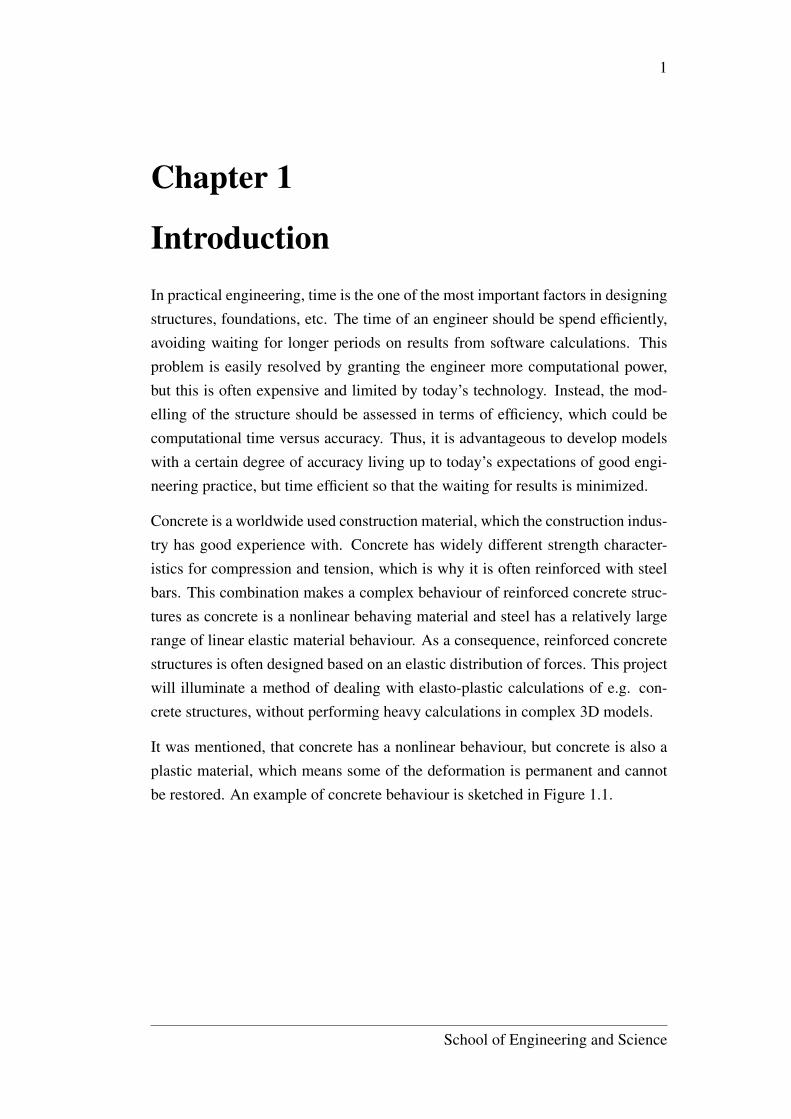
It was mentioned, that concrete has a nonlinear behaviour, but concrete is also aplastic material, which means some of the deformation is permanent and cannotbe restored. An example of concrete behaviour is sketched in Figure 1.1.
School of Engineering and Science
2 Chapter 1. Introduction
ε
σ
f t
εt ε
σ
E0A
Et
≈ 0.002
f c
εc εu
Com
pressive S
tress
Tensile S
tress
PR
OD
UC
ED
B
Y A
N A
UT
OD
ES
K E
DU
CA
TIO
NA
L P
RO
DU
CT
PRODUCED BY AN AUTODESK EDUCATIONAL PRODUCT
PR
OD
UC
ED
B
Y A
N A
UT
OD
ES
K E
DU
CA
TIO
NA
L P
RO
DU
CT
PRODUCED BY AN AUTODESK EDUCATIONAL PRODUCT
Figure 1.1: Stress - strain curves, Concrete.
The real behaviour of concrete is indicated by the red lines, where the blue linesare simplifications. First, the simplifications are applied to model the behaviourof concrete. Later on, the real behaviour is modelled via more complex materialmodels like Drucker-Prager.
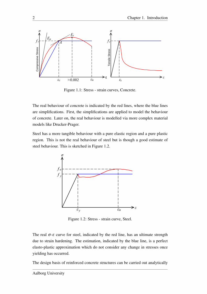
Steel has a more tangible behaviour with a pure elastic region and a pure plasticregion. This is not the real behaviour of steel but is though a good estimate ofsteel behaviour. This is sketched in Figure 1.2.
ε
σ
f y
εy εu
f u
PR
OD
UC
ED
B
Y A
N A
UT
OD
ES
K E
DU
CA
TIO
NA
L P
RO
DU
CT
PRODUCED BY AN AUTODESK EDUCATIONAL PRODUCT
PR
OD
UC
ED
B
Y A
N A
UT
OD
ES
K E
DU
CA
TIO
NA
L P
RO
DU
CT
PRODUCED BY AN AUTODESK EDUCATIONAL PRODUCT
Figure 1.2: Stress - strain curve, Steel.
The real σ -ε curve for steel, indicated by the red line, has an ultimate strengthdue to strain hardening. The estimation, indicated by the blue line, is a perfectelasto-plastic approximation which do not consider any change in stresses onceyielding has occurred.
The design basis of reinforced concrete structures can be carried out analytically
Aalborg University
Chapter 1. Introduction 3
as well as for many other types of materials. Analytical solutions are often fasterexecuted and easier to handle than complex numerical models. Also, analyti-cal approaches are widely used and accepted as applicable methods of designingstructures.
The material models shown earlier are not normally applicable in the beam el-ement method. Thus, an elasto-plastic beam element is implemented to handleplastic behaviour. This beam element also includes the possibility of applyingasymmetric cross sections.
Project description
This project can roughly be divided into two parts. Firstly, the main part is devel-oping a program in MatLab capable of calculating reinforced concrete structuresby use of one-dimensional finite element models. one-dimensional models areoften carried out by use of beam elements in terms of Bernoulli-Euler or Timo-shenko assumptions, and this is also the case in this project.
The MatLab program will then be compared with other methods of analysing re-inforced concrete structures. These other approaches will be an analytical methodand a numerical three-dimensional method by using Abaqus, which is a commer-cial software for analysing structures by the finite element method.
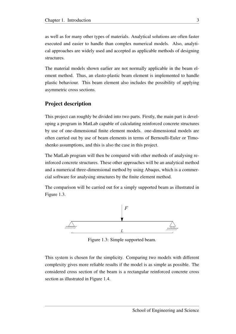
The comparison will be carried out for a simply supported beam as illustrated inFigure 1.3.
F
h
b
c
z
y
L
PR
OD
UC
ED
B
Y A
N A
UT
OD
ES
K E
DU
CA
TIO
NA
L P
RO
DU
CT
PRODUCED BY AN AUTODESK EDUCATIONAL PRODUCT
PR
OD
UC
ED
B
Y A
N A
UT
OD
ES
K E
DU
CA
TIO
NA
L P
RO
DU
CT
PRODUCED BY AN AUTODESK EDUCATIONAL PRODUCT
Figure 1.3: Simple supported beam.
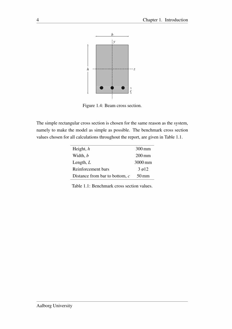
This system is chosen for the simplicity. Comparing two models with differentcomplexity gives more reliable results if the model is as simple as possible. Theconsidered cross section of the beam is a rectangular reinforced concrete crosssection as illustrated in Figure 1.4.
School of Engineering and Science
4 Chapter 1. Introduction
F
h
b
c
z
y
L
PR
OD
UC
ED
B
Y A
N A
UT
OD
ES
K E
DU
CA
TIO
NA
L P
RO
DU
CT
PRODUCED BY AN AUTODESK EDUCATIONAL PRODUCT
PR
OD
UC
ED
B
Y A
N A
UT
OD
ES
K E
DU
CA
TIO
NA
L P
RO
DU
CT
PRODUCED BY AN AUTODESK EDUCATIONAL PRODUCT
Figure 1.4: Beam cross section.
The simple rectangular cross section is chosen for the same reason as the system,namely to make the model as simple as possible. The benchmark cross sectionvalues chosen for all calculations throughout the report, are given in Table 1.1.
Height, h 300 mmWidth, b 200 mmLength, L 3000 mmReinforcement bars 3 ø12Distance from bar to bottom, c 50 mm
Table 1.1: Benchmark cross section values.
Aalborg University
Part I
Static finite-element analysis

7
Chapter 2
Beam theoryThe Bernoulli-Euler beam theory forms the basic foundation of the calculationsmade throughout most of this report.
2.1 Bernoulli-Euler beam theory
In this section the Bernoulli-Euler beam theory in incremental formulation withan arbitrary beam axis is present. First of all the basic assumption is stated thatplane sections remain plane and perpendicular to the neutral axis. Thus, no sheardeformation is considered.
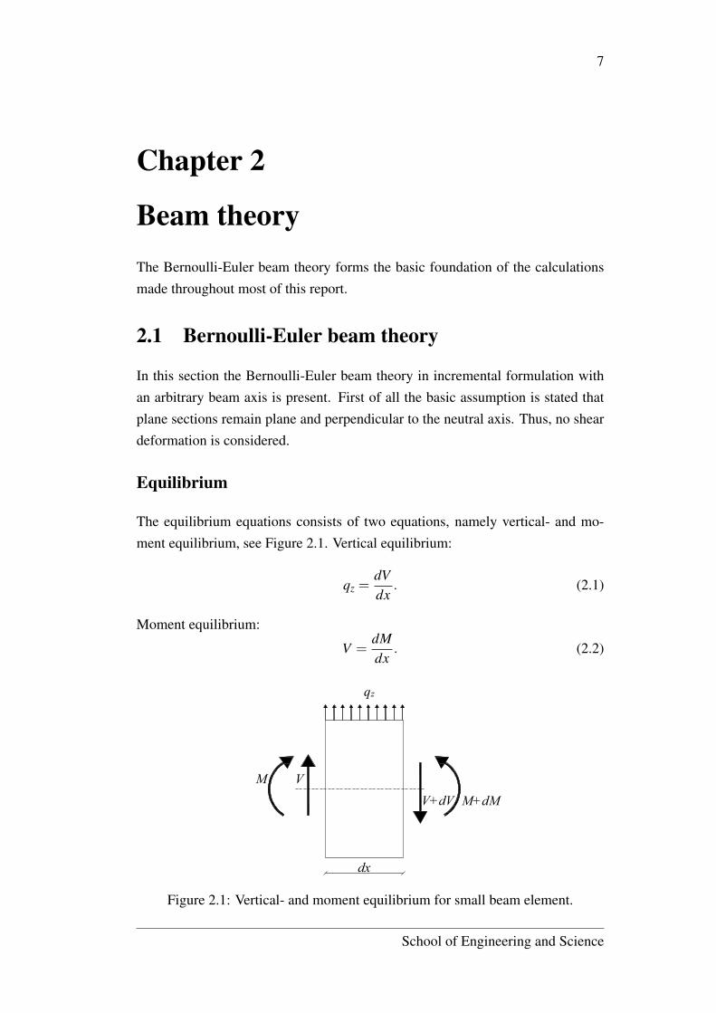
Equilibrium
The equilibrium equations consists of two equations, namely vertical- and mo-ment equilibrium, see Figure 2.1. Vertical equilibrium:
qz =dVdx
. (2.1)
Moment equilibrium:
V =dMdx
. (2.2)
dx
qz
M+dMM V
V+dV
PR
OD
UC
ED
B
Y A
N A
UT
OD
ES
K E
DU
CA
TIO
NA
L P
RO
DU
CT
PRODUCED BY AN AUTODESK EDUCATIONAL PRODUCT
PR
OD
UC
ED
B
Y A
N A
UT
OD
ES
K E
DU
CA
TIO
NA
L P
RO
DU
CT
PRODUCED BY AN AUTODESK EDUCATIONAL PRODUCT
Figure 2.1: Vertical- and moment equilibrium for small beam element.
School of Engineering and Science
8 2.1. Bernoulli-Euler beam theory
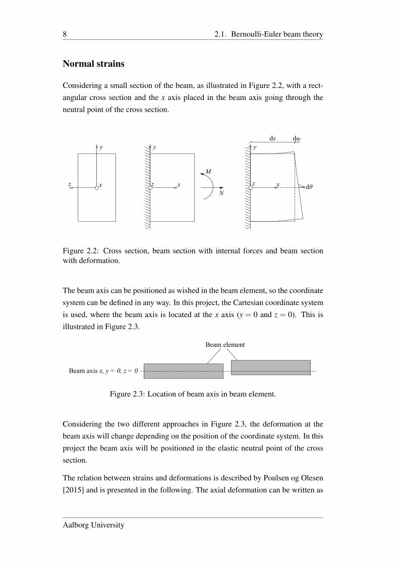
Normal strains
Considering a small section of the beam, as illustrated in Figure 2.2, with a rect-angular cross section and the x axis placed in the beam axis going through theneutral point of the cross section.
y
x xz
M
Nxz dθ
dx du0
dσ(y) dσ0 dσ(y) - dσ0
y y
z
Figure 2.2: Cross section, beam section with internal forces and beam sectionwith deformation.
The beam axis can be positioned as wished in the beam element, so the coordinatesystem can be defined in any way. In this project, the Cartesian coordinate systemis used, where the beam axis is located at the x axis (y = 0 and z = 0). This isillustrated in Figure 2.3.
As·f yc
Beam axis x, y = 0, z = 0
Beam element
Figure 2.3: Location of beam axis in beam element.
Considering the two different approaches in Figure 2.3, the deformation at thebeam axis will change depending on the position of the coordinate system. In thisproject the beam axis will be positioned in the elastic neutral point of the crosssection.
The relation between strains and deformations is described by Poulsen og Olesen[2015] and is presented in the following. The axial deformation can be written as
Aalborg University
2.1. Bernoulli-Euler beam theory 9
the displacement at the right edge of the beam section:
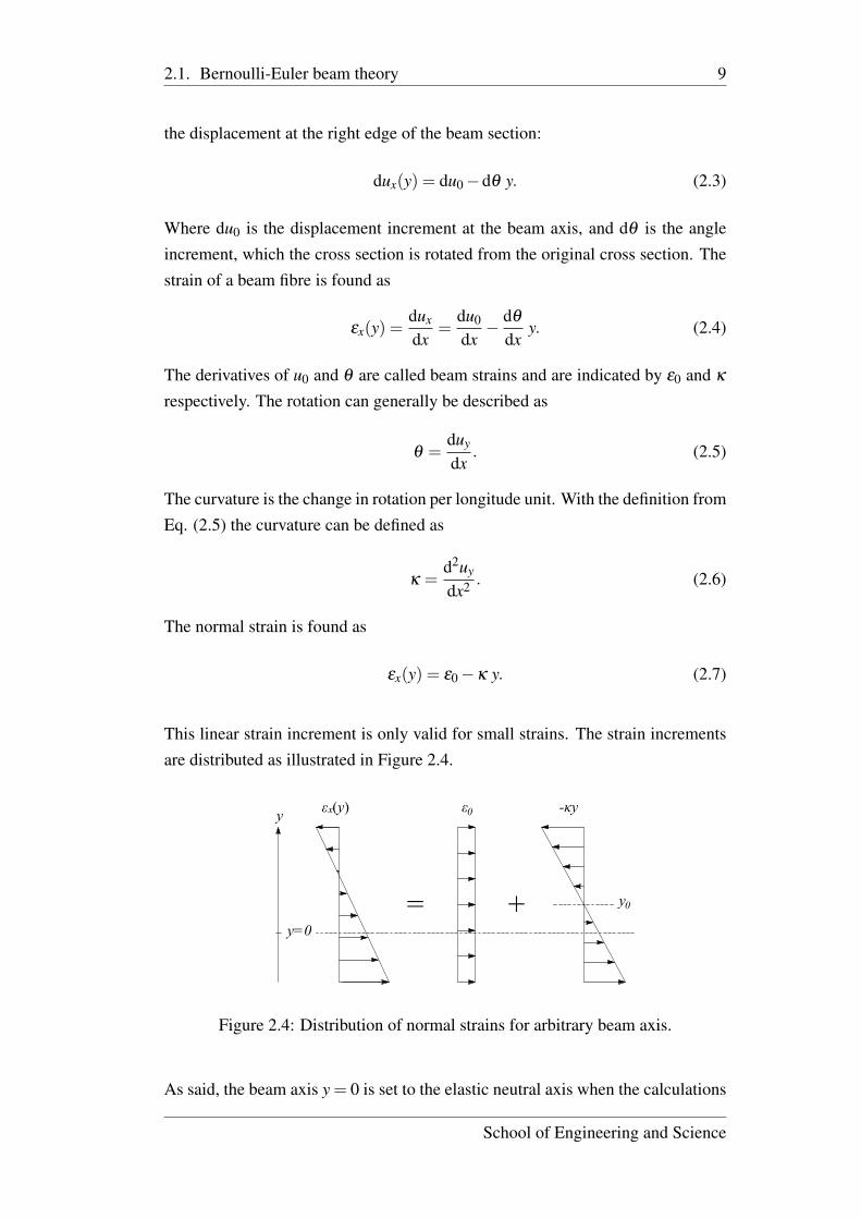
dux(y) = du0−dθ y. (2.3)
Where du0 is the displacement increment at the beam axis, and dθ is the angleincrement, which the cross section is rotated from the original cross section. Thestrain of a beam fibre is found as
εx(y) =dux
dx=
du0
dx− dθ
dxy. (2.4)
The derivatives of u0 and θ are called beam strains and are indicated by ε0 and κ
respectively. The rotation can generally be described as
θ =duy
dx. (2.5)
The curvature is the change in rotation per longitude unit. With the definition fromEq. (2.5) the curvature can be defined as
κ =d2uy
dx2 . (2.6)
The normal strain is found as
εx(y) = ε0−κ y. (2.7)
This linear strain increment is only valid for small strains. The strain incrementsare distributed as illustrated in Figure 2.4.
= +
εx(y) ε0 -κy
y=0
y
y0
Figure 2.4: Distribution of normal strains for arbitrary beam axis.
As said, the beam axis y = 0 is set to the elastic neutral axis when the calculations
School of Engineering and Science
10 2.1. Bernoulli-Euler beam theory
are initiated. This implies that y0 = 0, when the behaviour is elastic. When thematerial starts yielding y0 will differ from zero.
Normal stresses
For a linear elastic material the stress is given by Hooke’s law. The stress in abeam fibre can then be described as
σx(y) = E(y) εx(y) = E(y)(
dux
dx− dθz
dxy)= E(y) ε0−E(y) κy. (2.8)
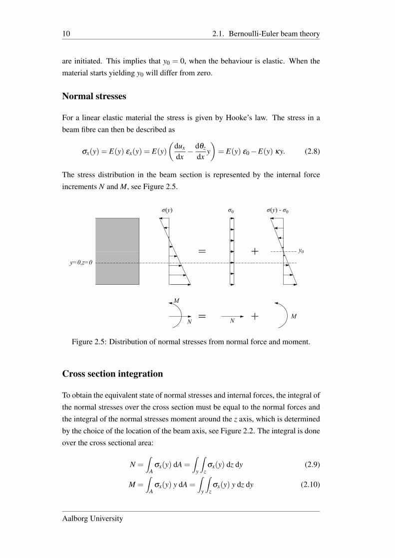
The stress distribution in the beam section is represented by the internal forceincrements N and M, see Figure 2.5.
= +
σ(y) σ0 σ(y) - σ0
M
N = +NM
y=0,z=0
y0
Figure 2.5: Distribution of normal stresses from normal force and moment.
Cross section integration
To obtain the equivalent state of normal stresses and internal forces, the integral ofthe normal stresses over the cross section must be equal to the normal forces andthe integral of the normal stresses moment around the z axis, which is determinedby the choice of the location of the beam axis, see Figure 2.2. The integral is doneover the cross sectional area:
N =∫
Aσx(y) dA =
∫y
∫zσx(y) dz dy (2.9)
M =∫
Aσx(y) y dA =
∫y
∫zσx(y) y dz dy (2.10)
Aalborg University
2.1. Bernoulli-Euler beam theory 11
For elastic cases, the relations can be expanded to
N =∫
y
∫z(E ε0−E κy) dz dy
=
(E A
dux
dx−∫
AE y dA
dθz
dx
), (2.11)
M =∫
y
∫z(E ε0−E κy) y dz dy
=
(−∫
AE y dA
dux
dx−∫
AE y2 dA
dθz
dx
). (2.12)
For plastic cases, an incremental formulation can be applied:
dN =∫
y
∫z(Et dε0−Et dκ y) dz dy (2.13)
dM =∫
y
∫z(Et dε0−Et dκ y) y dz dy. (2.14)
Only normal force dN and bending moment dM are found. The shear force mustbe found be equilibrium and is not related to the beam strains.
The integral of the stresses caused by bending must be equal to zero:∫A(σx(y)−σ0) dA =
∫A
Et (−κ y) dA = 0, (2.15)
where σ0 is the stress at the beam axis y = 0. The integral of the stresses causedby axial deformation must be equal to the normal force:
dN =∫
AEt dε0 dA. (2.16)
Governing equations
Combining the above relations and definitions of equilibrium, cross section inte-gration, material law and kinematics, the governing equation for the beam can be
School of Engineering and Science
12 2.1. Bernoulli-Euler beam theory
expressed as:
Rotation (Kinematic condition): θ =duy
dx, (2.17)
Bending moment (Static equivalence): M =∫
yE y2 dy
d2uy
dx2 , (2.18)
Shear force (Static equivalence): V =∫
yE y2 dy
d3uy
dx3 , (2.19)
Loading (Differential equation): qz =∫
yE y2 dy
d4uy
dx4 . (2.20)
On matrix form this can be presented asN
M
=
∫A E dA −
∫A Ey dA
−∫
A Ey dA∫
A Ey2 dA
duxdxdθzdx
. (2.21)
With these equations it is possible to analyse a beam by a fully analytical ap-proach.
Material law and material models
Plasticity is described as non-recoveable deformation of the material and leavespermanent strains in the beam when it is unloaded. Thus, Hooke’s law is notsufficient to describe the behaviour. An assumption can be made, as mentionedin Chapter 1, to describe the material elasto-plasticly. The material now behaveslinear elastic until yielding and then becomes perfect plastic. This is a good wayof describing steel behaviour without drifting to far from the real behaviour. Forconcrete, it is still a rough assumption to assume linear elastic - perfectly plasticbehaviour.
Drucker-Prager criterion
Constructing more realistic material models for concrete can be done by use ofmaterial models like Drucker-Prager. Krabbenhøft [2002] describes the Drucker-Prager criterion as a modified von Mises criterion:
f (I1,J2) =√
J2 +αI1− k. (2.22)
Aalborg University
2.1. Bernoulli-Euler beam theory 13
Where I1 and J2 are invariants and α , k are material parameters. The Drucker-Prager may also be written in terms of stresses:
f (σ) = σe +ασm−σ0. (2.23)
Where σe is the equivalent stress, σ0 is uniaxial yield stress and σm is the meanstress. The mean stress is given by:
σm = I1 =13(σx +σy +σz). (2.24)
The modification compared to the von Mises criterion allows setting a limit forpositive mean stresses, which is tensile stresses. The material is on the other handstrengthened by superposition of the negative mean stress.
Yield surface
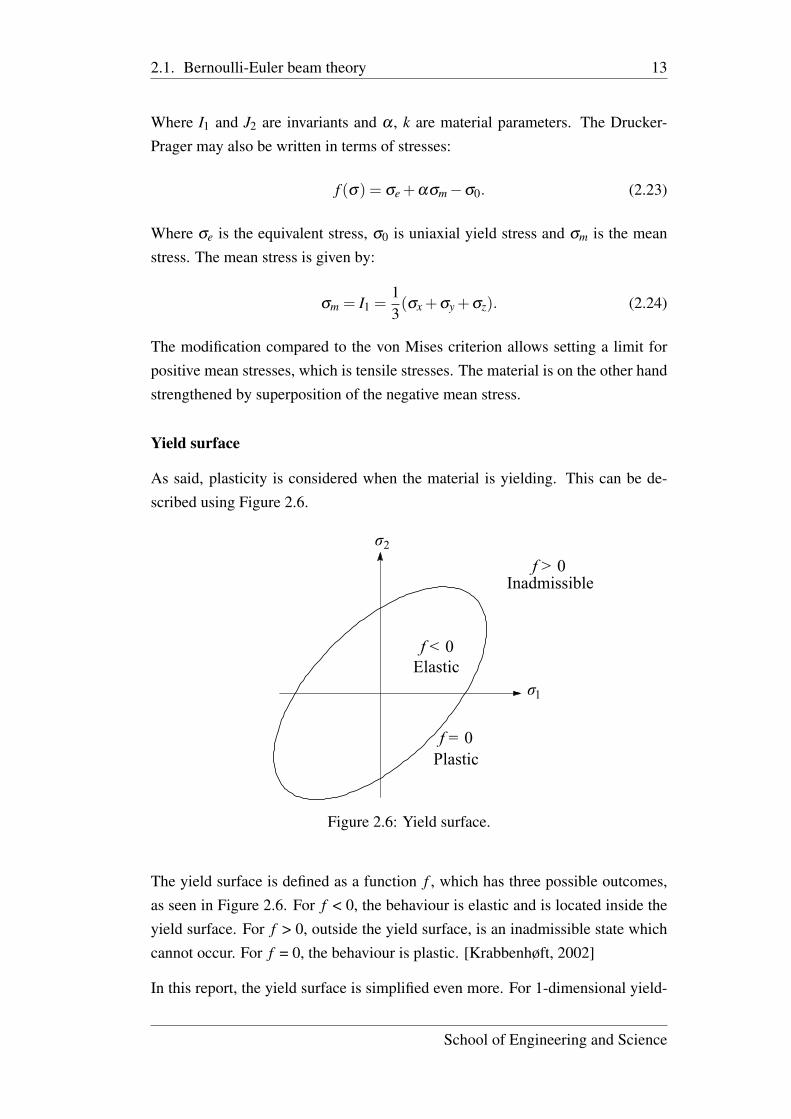
As said, plasticity is considered when the material is yielding. This can be de-scribed using Figure 2.6.
σ1
σ2
f = 0
f < 0
f > 0
Plastic
Elastic
Inadmissible
Figure 2.6: Yield surface.
The yield surface is defined as a function f , which has three possible outcomes,as seen in Figure 2.6. For f < 0, the behaviour is elastic and is located inside theyield surface. For f > 0, outside the yield surface, is an inadmissible state whichcannot occur. For f = 0, the behaviour is plastic. [Krabbenhøft, 2002]
In this report, the yield surface is simplified even more. For 1-dimensional yield-
School of Engineering and Science
14 2.2. Elasto-plastic bending
ing, the uniaxial yielding limits are sufficient to describe the behaviour. Thus,only compressive yielding and tensile yielding are needed to defined the yielding"surface". Thus, the Drucker-Prager criterion is not applied directly, but only theconcept is used to model the material behaviour in this project.
2.2 Elasto-plastic bending
When beams are loaded beyond their yield strength, plastic behaviour will occuras stated earlier, see Figure 1.2. The simplest case of yielding is obtained byobserving an axially loaded bar. In this case all points in the bar are subjected tothe same stress, which leads to simultaneous yielding throughout the bar.
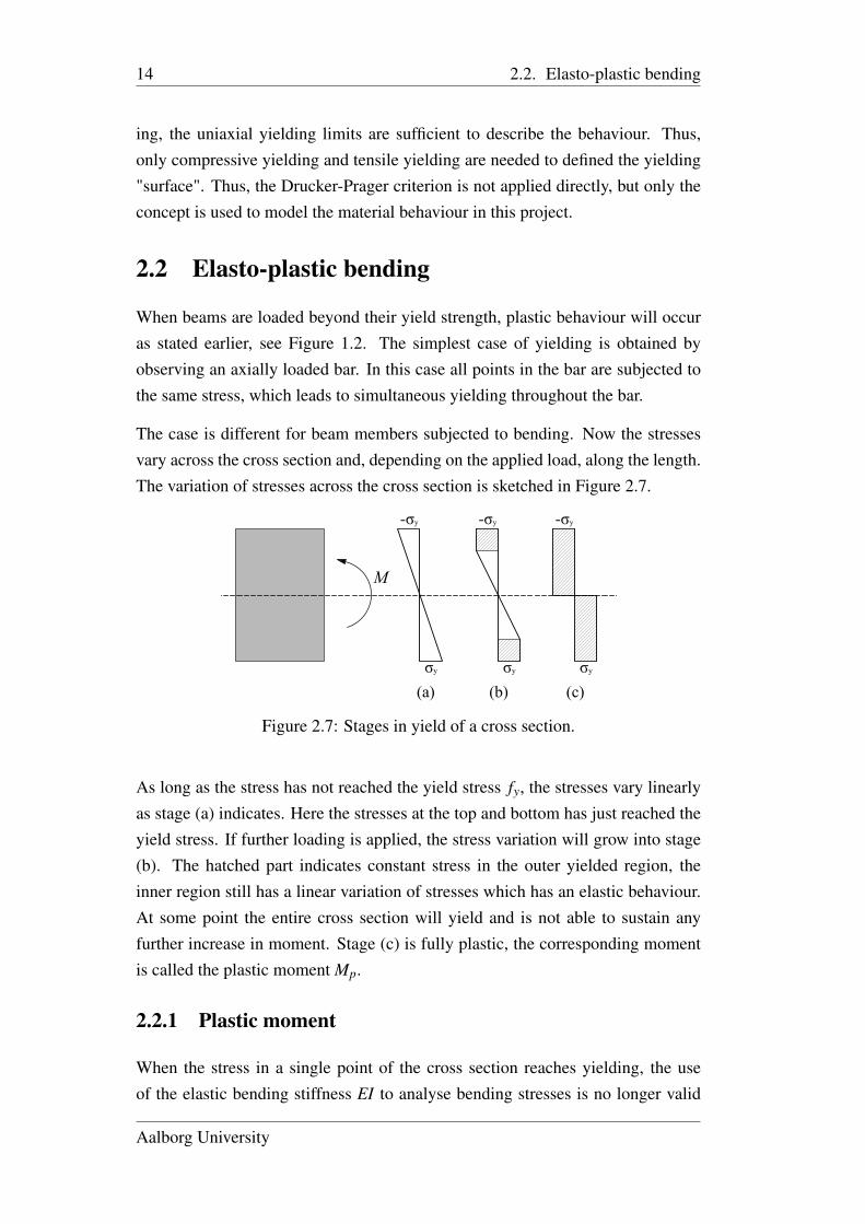
The case is different for beam members subjected to bending. Now the stressesvary across the cross section and, depending on the applied load, along the length.The variation of stresses across the cross section is sketched in Figure 2.7.
σy
-σy
σy
-σy
σy
-σy
(a) (b) (c)
M
Figure 2.7: Stages in yield of a cross section.
As long as the stress has not reached the yield stress fy, the stresses vary linearlyas stage (a) indicates. Here the stresses at the top and bottom has just reached theyield stress. If further loading is applied, the stress variation will grow into stage(b). The hatched part indicates constant stress in the outer yielded region, theinner region still has a linear variation of stresses which has an elastic behaviour.At some point the entire cross section will yield and is not able to sustain anyfurther increase in moment. Stage (c) is fully plastic, the corresponding momentis called the plastic moment Mp.
2.2.1 Plastic moment
When the stress in a single point of the cross section reaches yielding, the useof the elastic bending stiffness EI to analyse bending stresses is no longer valid
Aalborg University
2.2. Elasto-plastic bending 15
as the assumption of complete linear elastic cross section is violated. Instead,the moments of the cross section are used to analyse the bending stresses. Thissection is based on [Williams og Todd, 1999].
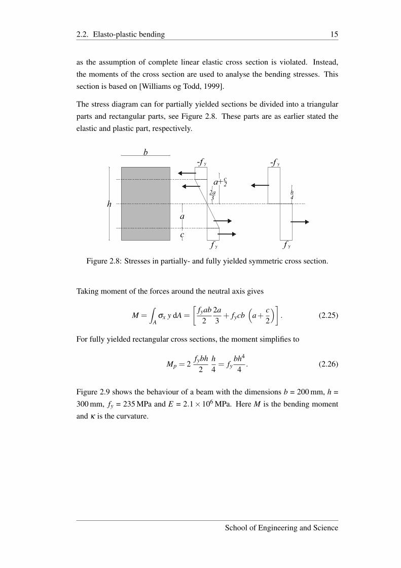
The stress diagram can for partially yielded sections be divided into a triangularparts and rectangular parts, see Figure 2.8. These parts are as earlier stated theelastic and plastic part, respectively.
f y
-f y
f y
-f y
a
c
2a3
a+ .c2
h
b
h4
Figure 2.8: Stresses in partially- and fully yielded symmetric cross section.
Taking moment of the forces around the neutral axis gives
M =∫
Aσx y dA =
[fyab
22a3+ fycb
(a+
c2
)]. (2.25)
For fully yielded rectangular cross sections, the moment simplifies to
Mp = 2fybh
2h4= fy
bh4
4. (2.26)
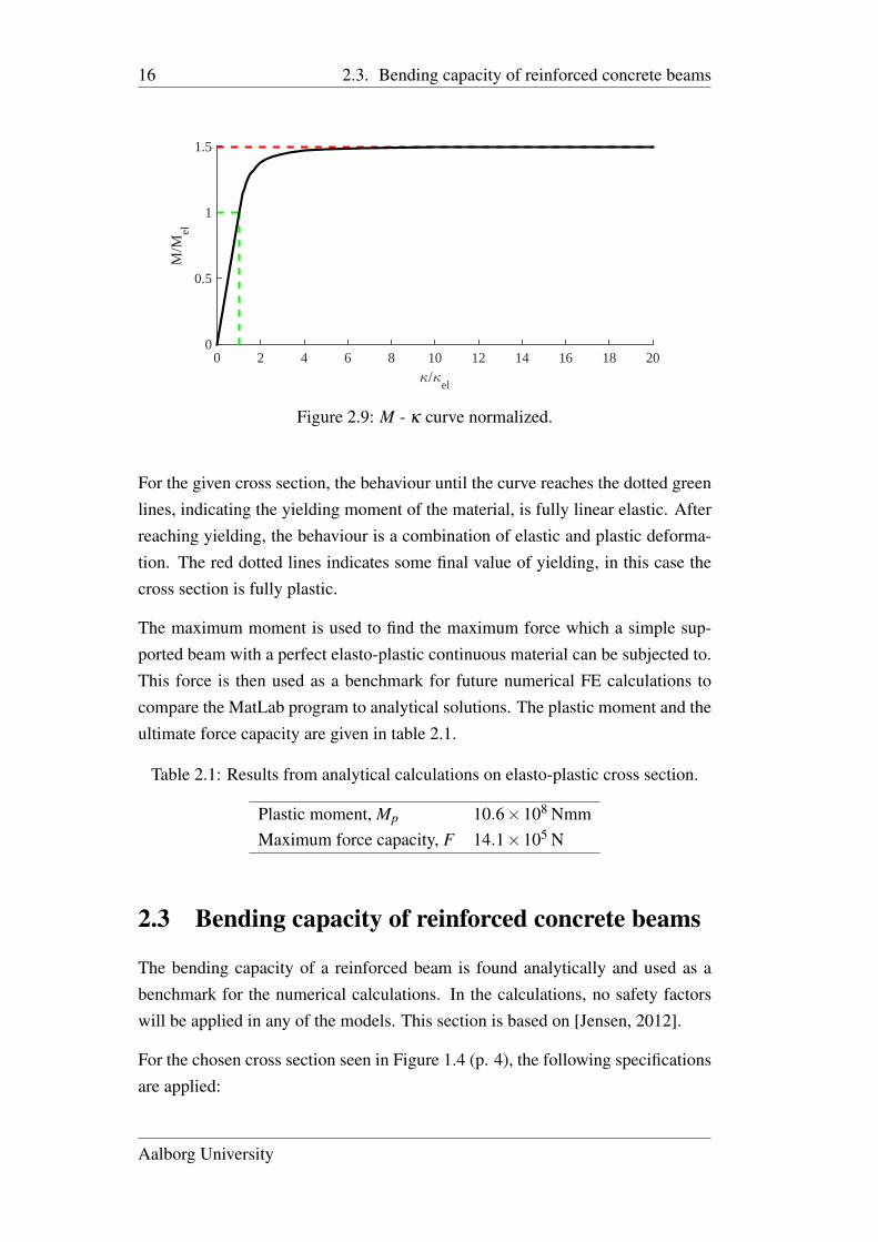
Figure 2.9 shows the behaviour of a beam with the dimensions b = 200 mm, h =300 mm, fy = 235 MPa and E = 2.1×10⁶ MPa. Here M is the bending momentand κ is the curvature.
School of Engineering and Science
16 2.3. Bending capacity of reinforced concrete beams
5/5el
0 2 4 6 8 10 12 14 16 18 20
M/M
el
0
0.5
1
1.5
Figure 2.9: M - κ curve normalized.
For the given cross section, the behaviour until the curve reaches the dotted greenlines, indicating the yielding moment of the material, is fully linear elastic. Afterreaching yielding, the behaviour is a combination of elastic and plastic deforma-tion. The red dotted lines indicates some final value of yielding, in this case thecross section is fully plastic.
The maximum moment is used to find the maximum force which a simple sup-ported beam with a perfect elasto-plastic continuous material can be subjected to.This force is then used as a benchmark for future numerical FE calculations tocompare the MatLab program to analytical solutions. The plastic moment and theultimate force capacity are given in table 2.1.
Table 2.1: Results from analytical calculations on elasto-plastic cross section.
Plastic moment, Mp 10.6×10⁸ NmmMaximum force capacity, F 14.1×10⁵ N
2.3 Bending capacity of reinforced concrete beams
The bending capacity of a reinforced beam is found analytically and used as abenchmark for the numerical calculations. In the calculations, no safety factorswill be applied in any of the models. This section is based on [Jensen, 2012].
For the chosen cross section seen in Figure 1.4 (p. 4), the following specificationsare applied:
Aalborg University
2.3. Bending capacity of reinforced concrete beams 17
Table 2.2: Beam properties.
Yield strength fc/ ft Young’s modulus EConcrete 30 MPa / 3 MPa 30×103 MPaSteel 550 MPa 210×103 MPa
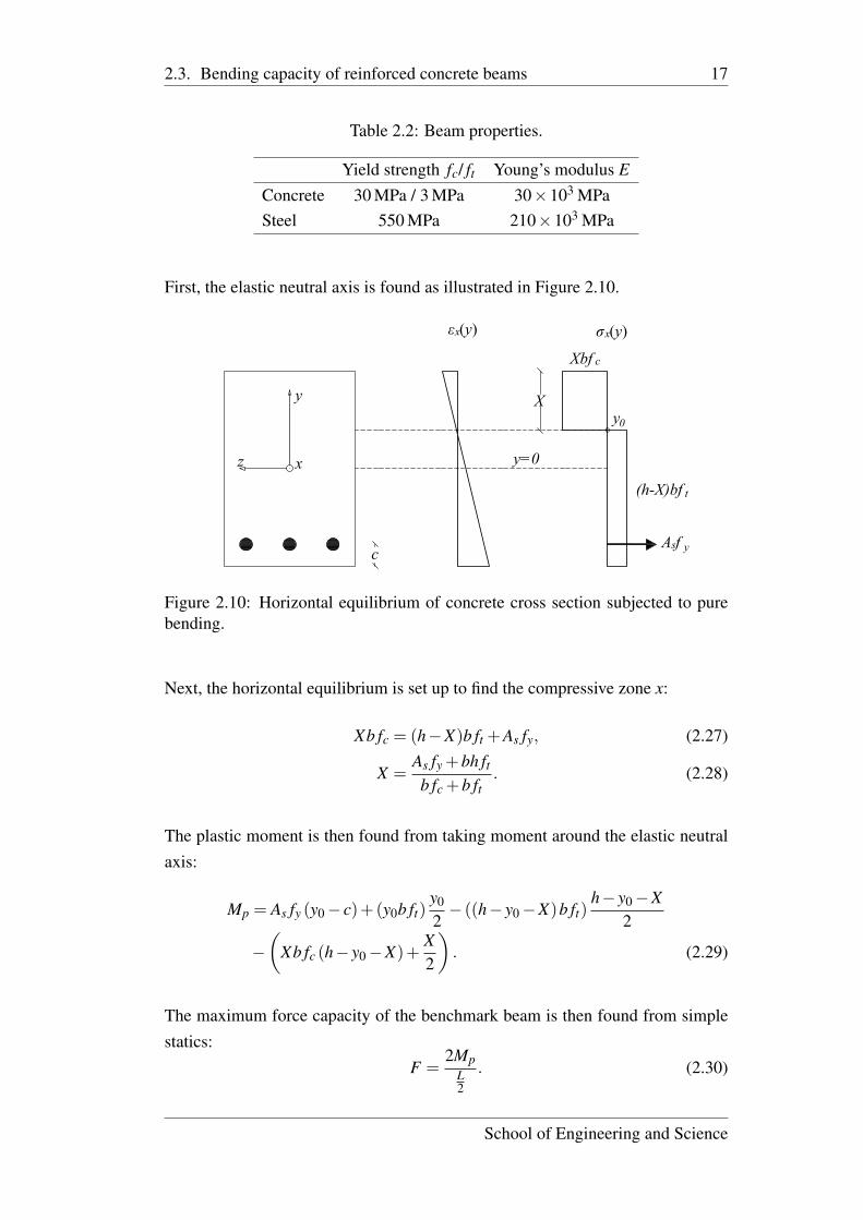
First, the elastic neutral axis is found as illustrated in Figure 2.10.
Asf y
Xbf c
(h-X)bf t
y0
X
c
εx(y) σx(y)
y=0
y
xz
Figure 2.10: Horizontal equilibrium of concrete cross section subjected to purebending.
Next, the horizontal equilibrium is set up to find the compressive zone x:
Xb fc = (h−X)b ft +As fy, (2.27)
X =As fy +bh ftb fc +b ft
. (2.28)
The plastic moment is then found from taking moment around the elastic neutralaxis:
Mp = As fy (y0− c)+(y0b ft)y0
2− ((h− y0−X)b ft)
h− y0−X2
−(
Xb fc (h− y0−X)+X2
). (2.29)
The maximum force capacity of the benchmark beam is then found from simplestatics:
F =2Mp
L2
. (2.30)
School of Engineering and Science

18 2.3. Bending capacity of reinforced concrete beams
The force F is the benchmark for the future numerical calculations on a concreteFE beam. Using the beam properties stated in Table 2.2, the compressive zone,plastic moment and maximum force capacity are calculated. The values are statedin Table 2.3.
Table 2.3: Results from analytical calculations.
Compressive zone, X 55.5 mmPlastic moment, Mp 6.3×10⁷ NmmMaximum force capacity, F 8.5×10⁴ N
Aalborg University
19
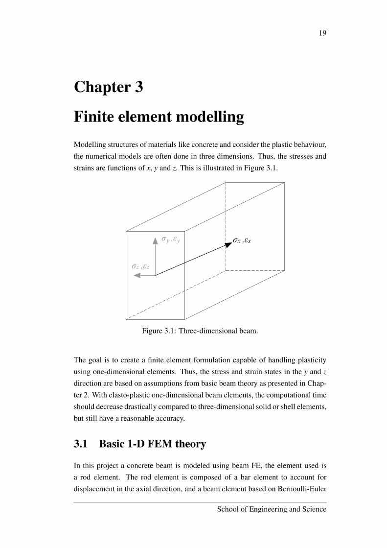
Chapter 3
Finite element modellingModelling structures of materials like concrete and consider the plastic behaviour,the numerical models are often done in three dimensions. Thus, the stresses andstrains are functions of x, y and z. This is illustrated in Figure 3.1.
σx ,εxσy ,εy
σz ,εz
Figure 3.1: Three-dimensional beam.
The goal is to create a finite element formulation capable of handling plasticityusing one-dimensional elements. Thus, the stress and strain states in the y and z
direction are based on assumptions from basic beam theory as presented in Chap-ter 2. With elasto-plastic one-dimensional beam elements, the computational timeshould decrease drastically compared to three-dimensional solid or shell elements,but still have a reasonable accuracy.
3.1 Basic 1-D FEM theory
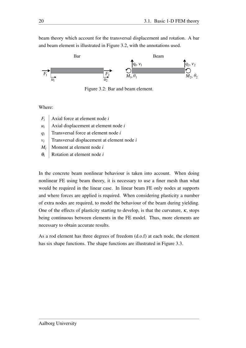
In this project a concrete beam is modeled using beam FE, the element used isa rod element. The rod element is composed of a bar element to account fordisplacement in the axial direction, and a beam element based on Bernoulli-Euler
School of Engineering and Science
20 3.1. Basic 1-D FEM theory
beam theory which account for the transversal displacement and rotation. A barand beam element is illustrated in Figure 3.2, with the annotations used.
u1 u2
F1 F2 M2, θ2M1, θ1
q2, v2q1 v1
Bar Beam,
Figure 3.2: Bar and beam element.
Where:
Fi Axial force at element node iui Axial displacement at element node iqi Transversal force at element node ivi Transversal displacement at element node iMi Moment at element node iθi Rotation at element node i
In the concrete beam nonlinear behaviour is taken into account. When doingnonlinear FE using beam theory, it is necessary to use a finer mesh than whatwould be required in the linear case. In linear beam FE only nodes at supportsand where forces are applied is required. When considering plasticity a numberof extra nodes are required, to model the behaviour of the beam during yielding.One of the effects of plasticity starting to develop, is that the curvature, κ , stopsbeing continuous between elements in the FE model. Thus, more elements arenecessary to obtain accurate results.
As a rod element has three degrees of freedom (d.o.f) at each node, the elementhas six shape functions. The shape functions are illustrated in Figure 3.3.
Aalborg University
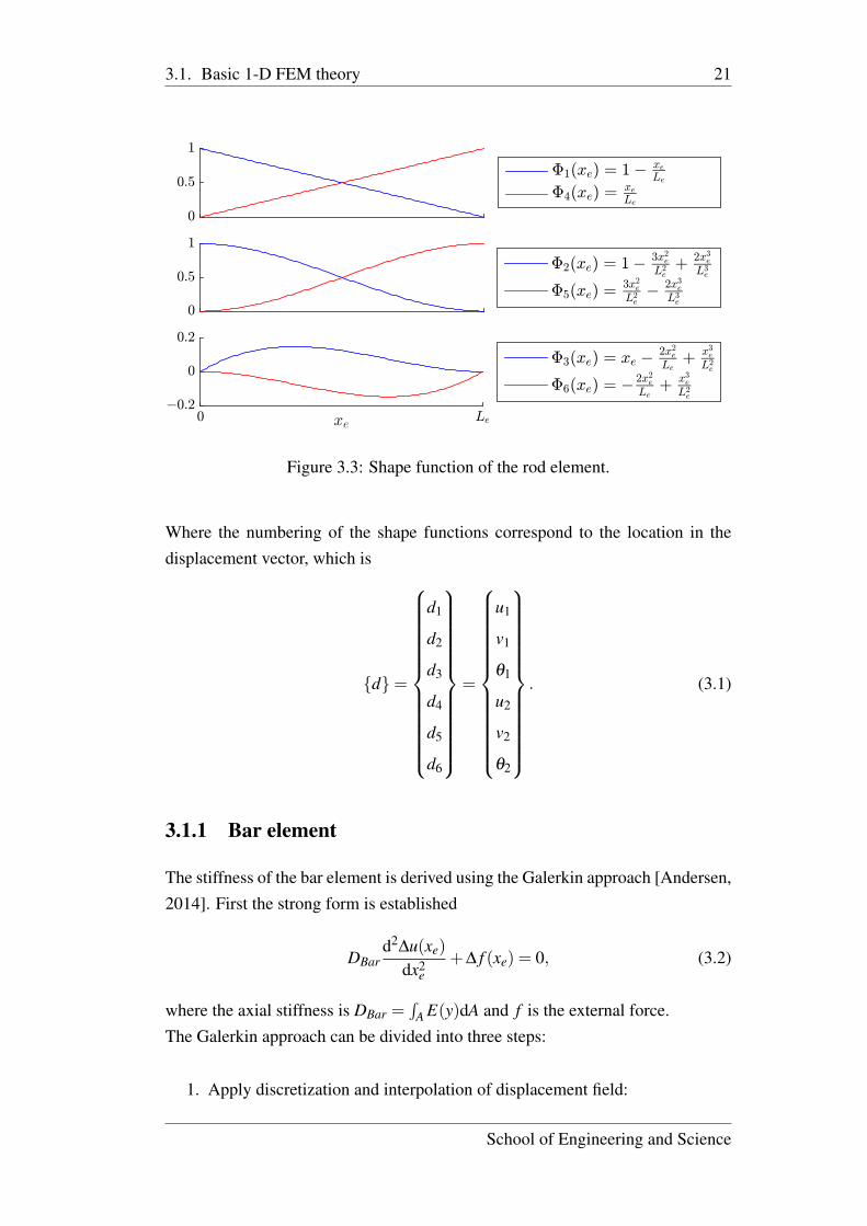
3.1. Basic 1-D FEM theory 21
0
0:5
1
)1(xe) = 1! xe
Le
)4(xe) = xe
Le
0
0:5
1
)2(xe) = 1! 3x2e
L2e
+ 2x3e
L3e
)5(xe) = 3x2e
L2e!
2x3e
L3e
xe
!0:2
0
0:2
0 Le
)3(xe) = xe !2x2
e
Le+ x3
e
L2e
)6(xe) = !2x2
e
Le+ x3
e
L2e
Figure 3.3: Shape function of the rod element.
Where the numbering of the shape functions correspond to the location in thedisplacement vector, which is
{d}=
d1
d2
d3
d4
d5
d6
=
u1
v1
θ1
u2
v2
θ2
. (3.1)
3.1.1 Bar element
The stiffness of the bar element is derived using the Galerkin approach [Andersen,2014]. First the strong form is established
DBard2
∆u(xe)
dx2e
+∆ f (xe) = 0, (3.2)
where the axial stiffness is DBar =∫
A E(y)dA and f is the external force.The Galerkin approach can be divided into three steps:
1. Apply discretization and interpolation of displacement field:
School of Engineering and Science
22 3.1. Basic 1-D FEM theory
∆u(xe) = {Φ(xe)}{∆d}
DBard2{Φ(xe)}
dx2e{∆d}+∆ f (xe) = 0. (3.3)
Here only the shape functions corresponding to the bar element are used,{Φ(xe)}= {Φ1(xe) Φ4(xe)}.
2. Premultiply strong form by weight function: {Φ(xe)}T
{Φ(xe)}T(
DBard2{Φ(xe)}
dx2e{∆d}+∆ f (xe)
)= {Φ(xe)}T 0. (3.4)
3. Integrate by parts over the element length
∫ Le
0{Φ(xe)}T
(DBar
d2{Φ(xe)}dx2
e{∆d}+∆ f (xe)
)dx =∫ Le
0{Φ(xe)}T 0dx.⇒[
{Φ(xe)}T DBard{Φ(xe)}
dxe
]Le
0{∆d}− (3.5)∫ Le
0
d{Φ(xe)}T
dxeDBar
d{Φ(xe)}dxe
{∆d}dx+∫ Le
0{Φ(xe)}T
∆ f (xe)dx = {0}
The physical interpretation of the second term in Equation (3.5) is [k]{∆d}, so thestiffness becomes
[kBar] =∫ Le
0
d{Φ(xe)}T
dxeDBar
d{Φ(xe)}dxe
dx. (3.6)
This can be simplified to
[kBar] =∫ Le
0{BBar}T DBar{BBar}dx (3.7)
Where {BBar} is the strain interpolation vector of a bar element and DBar is theconstitutive relation in the bar. The first term in Equation (3.5) is the boundary
Aalborg University
3.1. Basic 1-D FEM theory 23
load.
{ fB}=[{Φ(xe)}T DBar
d{Φ(xe)}dxe
]Le
0{∆d} (3.8)
The third term is the consistent nodal loads, used to apply line loads.
{ fC}=∫ Le
0{Φ(xe)}T
∆ f (xe)dx (3.9)
The total load is the sum of the boundary load and the consistent nodal load,
{ fT}= { fB}+{ fC}. (3.10)
3.1.2 Beam element
The stiffness matrix of the beam element is derived using the Galerkin approach[Andersen, 2014]. First the strong form is established
DBeamd4
∆v(xe)
dx4e
= ∆ f (xe), (3.11)
where the bending stiffness is DBeam =∫
A E(y) y2 dA.
The Galerkin approach can be divided into three steps:
1. Apply discretization and interpolation of displacement field:∆v(xe) = {Φ(xe)}{∆d}
DBeamd4{Φ(xe)}
dx4e{∆d}−∆ f (xe) = 0. (3.12)
Here only the shape function corresponding to the beam element is used,which is rotation and transversal displacement,{Φ(xe)}= {Φ2(xe) Φ3(xe) Φ5(xe) Φ6(xe)}.
2. Premultiply strong form by weight function: {Φ(xe)}T
{Φ(xe)}T(
DBeamd4{Φ(xe)}
dx4e{∆d}−∆ f (xe)
)= {Φ(xe)}T 0. (3.13)
School of Engineering and Science
24 3.1. Basic 1-D FEM theory
3. Integrate by parts over the element length
∫ Le
0{Φ(xe)}T
(DBeam
d4{Φ(xe)}dx4
e{∆d}−∆ f (xe)
)dx =∫ Le
0{Φ(xe)}T 0dx⇒[
{Φ(xe)}T DBeamd3{Φ(xe)}
dx3e
]Le
0{∆d}+[
{Φ(xe)}T DBeamd2{Φ(xe)}
dx2e
]Le
0{∆d}− (3.14)∫ Le
0
d2{Φ(xe)}T
dx2e
DBeamd2{Φ(xe)}
dx2e
dx{∆d}−∫ Le
0{Φ(xe)}T
∆ f (xe)dx = {0}
The physical interpretation of the third term in Eq. (3.14) is [k]{d}, so the stiffnessbecomes
[kBeam] =∫ Le
0
d2{Φ(xe)}T
dx2e
DBeamd2{Φ(xe)}
dx2e
dx (3.15)
This can be simplified to
[kBeam] =∫ Le
0{BBeam}T DBeam{BBeam}dx (3.16)
Where {BBeam} is the strain interpolation vector of a beam element and DBeam isthe constitutive relation in the beam. The first and second term in Eq. (3.14) is theboundary loads.
{ fB}=[{Φ(xe)}T DBeam
d3{Φ(xe)}dx3
e
]Le
0{∆d}
+
[{Φ(xe)}T DBeam
d2{Φ(xe)}dx2
e
]Le
0{∆d} (3.17)
The fourth term is the consistent nodal loads, used to apply line loads.
{ fC}=∫ Le
0{Φ(xe)}T
∆ f (xe)dx (3.18)
Aalborg University
3.1. Basic 1-D FEM theory 25
The total load is the sum of the boundary load and the consistent nodal load,
{ fT}= { fB}+{ fC}. (3.19)
3.1.3 Rod element
To calculate the stiffness matrix for the rod element, the strain interpolation matrixand the constitutive matrix is needed. The strain interpolation vector of the bar andbeam element, is combined into a strain interpolation matrix for the rod element.
B =
BBar(1) 0 0 BBar(2) 0 0
0 BBeam(1) BBeam(2) 0 BBeam(3) BBeam(4)
(3.20)
The constitutive matrix for the rod element consist of the constitutive relation formthe bar and beam element, to account for a arbitrary beam axis a diagonal term isadded.
[D] =
DBar −∫
A E(y) y dA
−∫
A E(y) y dA DBeam
(3.21)
The stiffness matrix for the rod element is
[k] =∫ Le
0[B]T [D][B]dx. (3.22)
3.1.4 Quadrature methods
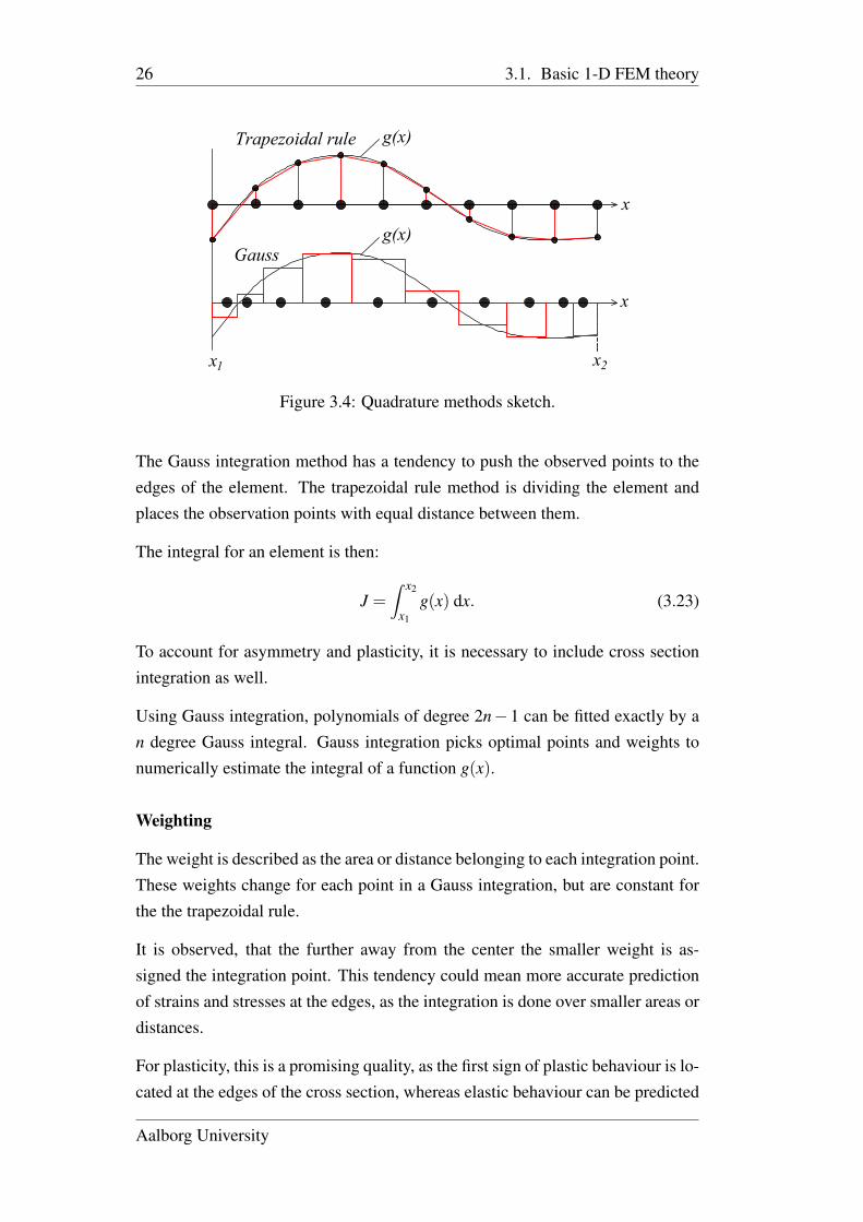
The choice of numerical integration method is a part of the program which hasinfluence on the accuracy and computing time. In this project two methods areused to handle numerical integration tasks. This being the trapezoidal rule andGauss integration. The difference is roughly sketched in Figure 3.4.
School of Engineering and Science
26 3.1. Basic 1-D FEM theory
x
x
Trapezoidal rule
Gauss
g(x)
g(x)
x1 x2
Figure 3.4: Quadrature methods sketch.
The Gauss integration method has a tendency to push the observed points to theedges of the element. The trapezoidal rule method is dividing the element andplaces the observation points with equal distance between them.
The integral for an element is then:
J =∫ x2
x1
g(x) dx. (3.23)
To account for asymmetry and plasticity, it is necessary to include cross sectionintegration as well.
Using Gauss integration, polynomials of degree 2n−1 can be fitted exactly by an degree Gauss integral. Gauss integration picks optimal points and weights tonumerically estimate the integral of a function g(x).
Weighting
The weight is described as the area or distance belonging to each integration point.These weights change for each point in a Gauss integration, but are constant forthe the trapezoidal rule.
It is observed, that the further away from the center the smaller weight is as-signed the integration point. This tendency could mean more accurate predictionof strains and stresses at the edges, as the integration is done over smaller areas ordistances.
For plasticity, this is a promising quality, as the first sign of plastic behaviour is lo-cated at the edges of the cross section, whereas elastic behaviour can be predicted
Aalborg University
3.2. Plasticity in FEM 27
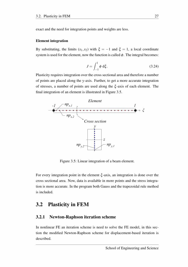
exact and the need for integration points and weights are less.
Element integration
By substituting, the limits (x1,x2) with ξ = −1 and ξ = 1, a local coordinatesystem is used for the element, now the function is called φ . The integral becomes:
J =∫ 1
−1φ dξ . (3.24)
Plasticity requires integration over the cross sectional area and therefore a numberof points are placed along the y-axis. Further, to get a more accurate integrationof stresses, a number of points are used along the ξ -axis of each element. Thefinal integration of an element is illustrated in Figure 3.5.
-1 1npx,1
npx,2
ξ
y
znpy,1npy,2
Element
Cross section
PR
OD
UC
ED
B
Y A
N A
UT
OD
ES
K E
DU
CA
TIO
NA
L P
RO
DU
CT
PRODUCED BY AN AUTODESK EDUCATIONAL PRODUCT
PR
OD
UC
ED
B
Y A
N A
UT
OD
ES
K E
DU
CA
TIO
NA
L P
RO
DU
CT
PRODUCED BY AN AUTODESK EDUCATIONAL PRODUCT
Figure 3.5: Linear integration of a beam element.
For every integration point in the element ξ -axis, an integration is done over thecross sectional area. Now, data is available in more points and the stress integra-tion is more accurate. In the program both Gauss and the trapezoidal rule methodis included.
3.2 Plasticity in FEM
3.2.1 Newton-Raphson iteration scheme
In nonlinear FE an iteration scheme is need to solve the FE model, in this sec-tion the modified Newton-Raphson scheme for displacement-based iteration isdescribed.
School of Engineering and Science
28 3.2. Plasticity in FEM
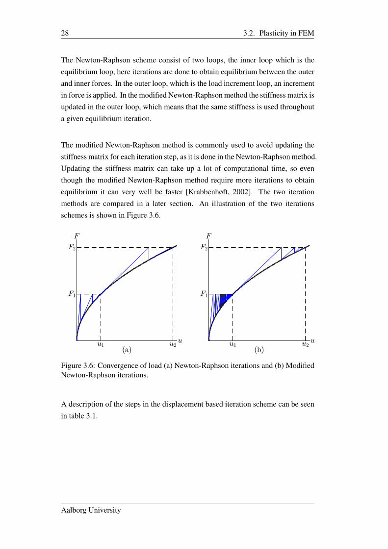
The Newton-Raphson scheme consist of two loops, the inner loop which is theequilibrium loop, here iterations are done to obtain equilibrium between the outerand inner forces. In the outer loop, which is the load increment loop, an incrementin force is applied. In the modified Newton-Raphson method the stiffness matrix isupdated in the outer loop, which means that the same stiffness is used throughouta given equilibrium iteration.
The modified Newton-Raphson method is commonly used to avoid updating thestiffness matrix for each iteration step, as it is done in the Newton-Raphson method.Updating the stiffness matrix can take up a lot of computational time, so eventhough the modified Newton-Raphson method require more iterations to obtainequilibrium it can very well be faster [Krabbenhøft, 2002]. The two iterationmethods are compared in a later section. An illustration of the two iterationsschemes is shown in Figure 3.6.
F1
F2
F
u1 u2u
(a)
F1
F2
F
u1 u2u
(b)
Figure 3.6: Convergence of load (a) Newton-Raphson iterations and (b) ModifiedNewton-Raphson iterations.
A description of the steps in the displacement based iteration scheme can be seenin table 3.1.
Aalborg University
3.2. Plasticity in FEM 29
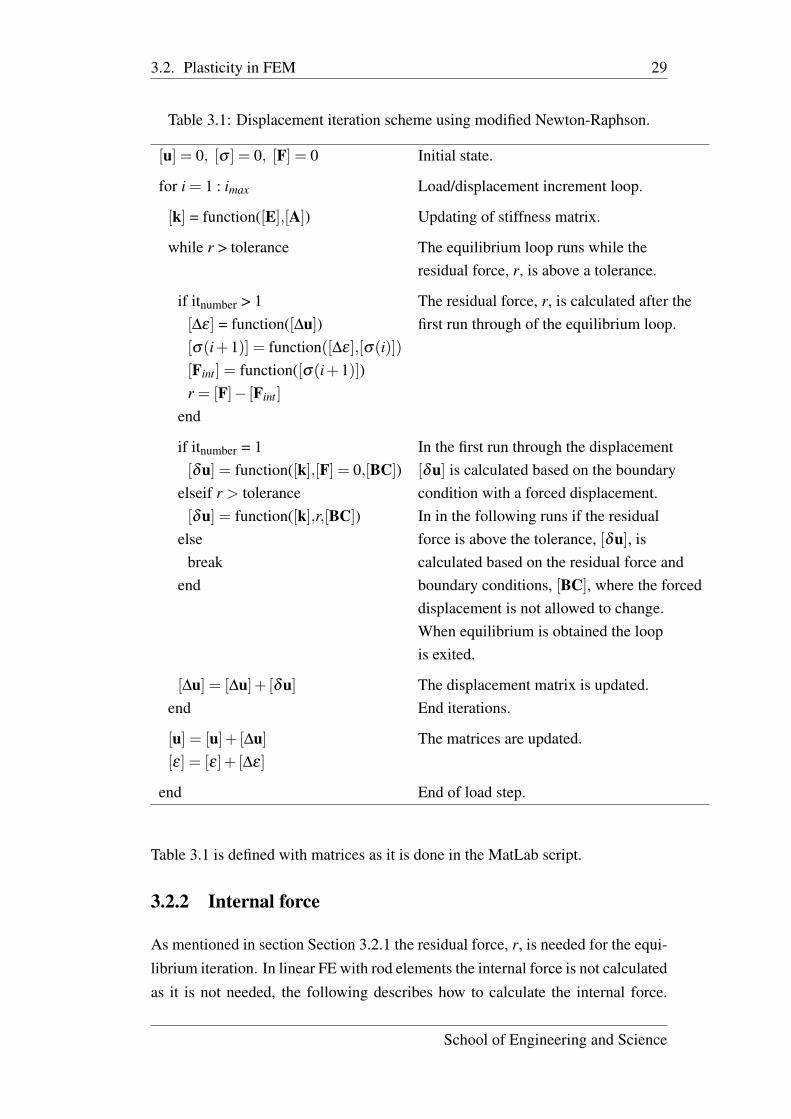
Table 3.1: Displacement iteration scheme using modified Newton-Raphson.
[u] = 0, [σ ] = 0, [F] = 0 Initial state.
for i = 1 : imax Load/displacement increment loop.
[k] = function([E],[A]) Updating of stiffness matrix.
while r > tolerance The equilibrium loop runs while theresidual force, r, is above a tolerance.
if itnumber > 1 The residual force, r, is calculated after the[∆ε] = function([∆u]) first run through of the equilibrium loop.[σ(i+1)] = function([∆ε],[σ(i)])[Fint ] = function([σ(i+1)])r = [F]− [Fint ]
end
if itnumber = 1 In the first run through the displacement[δu] = function([k],[F] = 0,[BC]) [δu] is calculated based on the boundary
elseif r > tolerance condition with a forced displacement.[δu] = function([k],r,[BC]) In in the following runs if the residual
else force is above the tolerance, [δu], isbreak calculated based on the residual force and
end boundary conditions, [BC], where the forceddisplacement is not allowed to change.When equilibrium is obtained the loopis exited.
[∆u] = [∆u]+ [δu] The displacement matrix is updated.end End iterations.
[u] = [u]+ [∆u] The matrices are updated.[ε] = [ε]+ [∆ε]
end End of load step.
Table 3.1 is defined with matrices as it is done in the MatLab script.
3.2.2 Internal force
As mentioned in section Section 3.2.1 the residual force, r, is needed for the equi-librium iteration. In linear FE with rod elements the internal force is not calculatedas it is not needed, the following describes how to calculate the internal force.
School of Engineering and Science
30 3.2. Plasticity in FEM
Based on the shape functions and the displacement, the strain can be obtained.The strains in a bar element and beam element is calculated in two different ways.
First the displacement vector in the global system is rotated to get the displace-ment vector in the local system.
{d′}= [T] {d} (3.25)
The transformation matrix is
[T] =
c s 0 0 0 0
−s c 0 0 0 0
0 0 1 0 0 0
0 0 0 c s 0
0 0 0 −s c 0
0 0 0 0 0 1
, (3.26)
and
c =d′4−d′1
Le, s =
d′5−d′2Le
. (3.27)
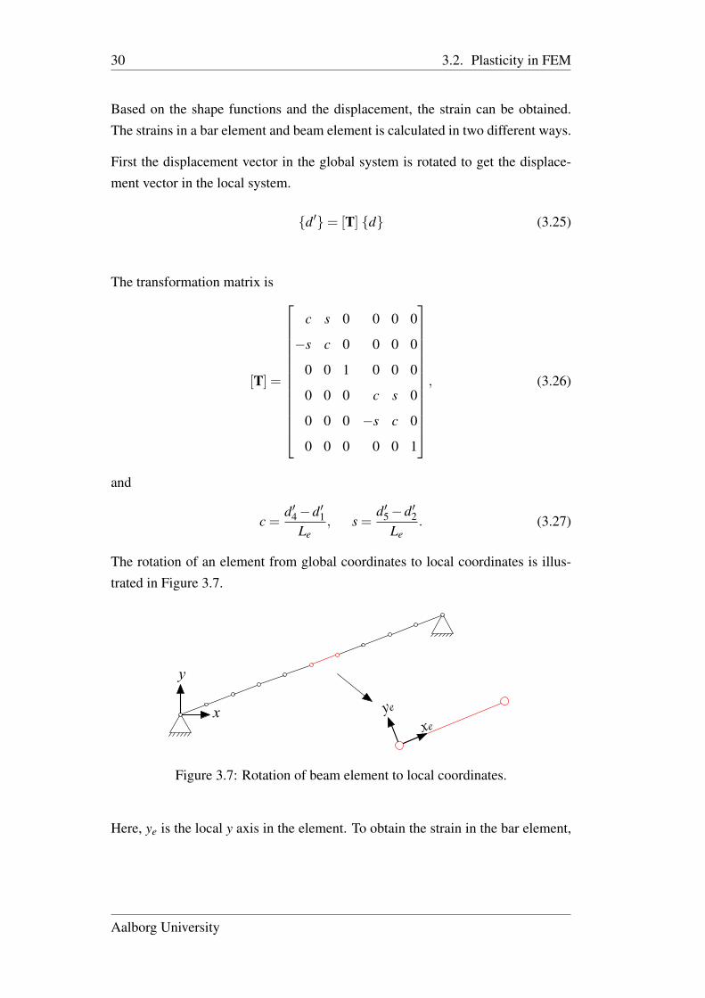
The rotation of an element from global coordinates to local coordinates is illus-trated in Figure 3.7.
y
x ye
xe
Figure 3.7: Rotation of beam element to local coordinates.
Here, ye is the local y axis in the element. To obtain the strain in the bar element,
Aalborg University
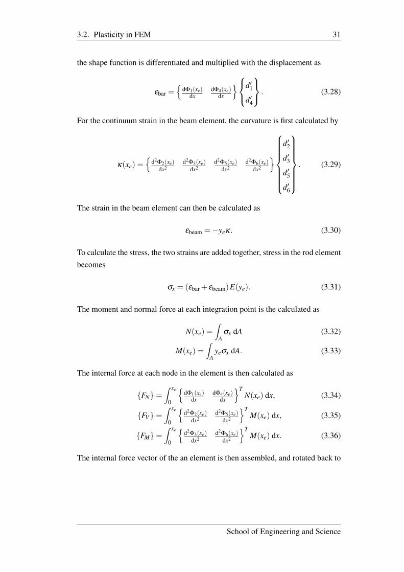
3.2. Plasticity in FEM 31
the shape function is differentiated and multiplied with the displacement as
εbar ={
dΦ1(xe)dx
dΦ4(xe)dx
}d′1
d′4
. (3.28)
For the continuum strain in the beam element, the curvature is first calculated by
κ(xe) ={
d2Φ2(xe)dx2
d2Φ3(xe)dx2
d2Φ5(xe)dx2
d2Φ6(xe)dx2
}
d′2
d′3
d′5d′6
. (3.29)
The strain in the beam element can then be calculated as
εbeam =−yeκ. (3.30)
To calculate the stress, the two strains are added together, stress in the rod elementbecomes
σx = (εbar + εbeam)E(ye). (3.31)
The moment and normal force at each integration point is the calculated as
N(xe) =∫
Aσx dA (3.32)
M(xe) =∫
Ayeσx dA. (3.33)
The internal force at each node in the element is then calculated as
{FN}=∫ xe
0
{dΦ1(xe)
dxdΦ4(xe)
dx
}TN(xe) dx, (3.34)
{FV}=∫ xe
0
{d2
Φ2(xe)dx2
d2Φ5(xe)dx2
}TM(xe) dx, (3.35)
{FM}=∫ xe
0
{d2
Φ3(xe)dx2
d2Φ6(xe)dx2
}TM(xe) dx. (3.36)
The internal force vector of the an element is then assembled, and rotated back to
School of Engineering and Science

32 3.2. Plasticity in FEM
global coordinates
{Fe}= T−1
FN,1
FV,1
FM,1
FN,2
FV,2
FM,2
(3.37)
The internal force vector can then be assembled, and the residual force, r = f −fint , calculated.
3.2.3 Elasto-plastic calculations on continuous cross section
Calculating a force/displacement curve for the beam model shows both the elasticregion and the ultimate force capacity of the beam. In Section 2.2.1, the plasticmoment was calculated. Using the plastic moment, the ultimate force capacity isfound.
In Figure 3.8, the force/displacement curve shows the force going towards theultimate analytically force capacity.
Displacement u [mm]0 2 4 6 8 10 12
Forc
e F
[N
]
#105
0
5
10
15
Analytical limitNumerical
Figure 3.8: F-u curve.
The applied mesh in the numerical model is so fine, that the model is converged,
Aalborg University
3.2. Plasticity in FEM 33
a convergence study is presented later in the report. As a result the deviationbetween the analytical solution and the numerical solution is very small. Thisproves, that it is possible to obtain the same result as the analytical solution, byapplying the one-dimensional finite element method for an elasto-plastic beam.
3.2.4 Effects of plasticity
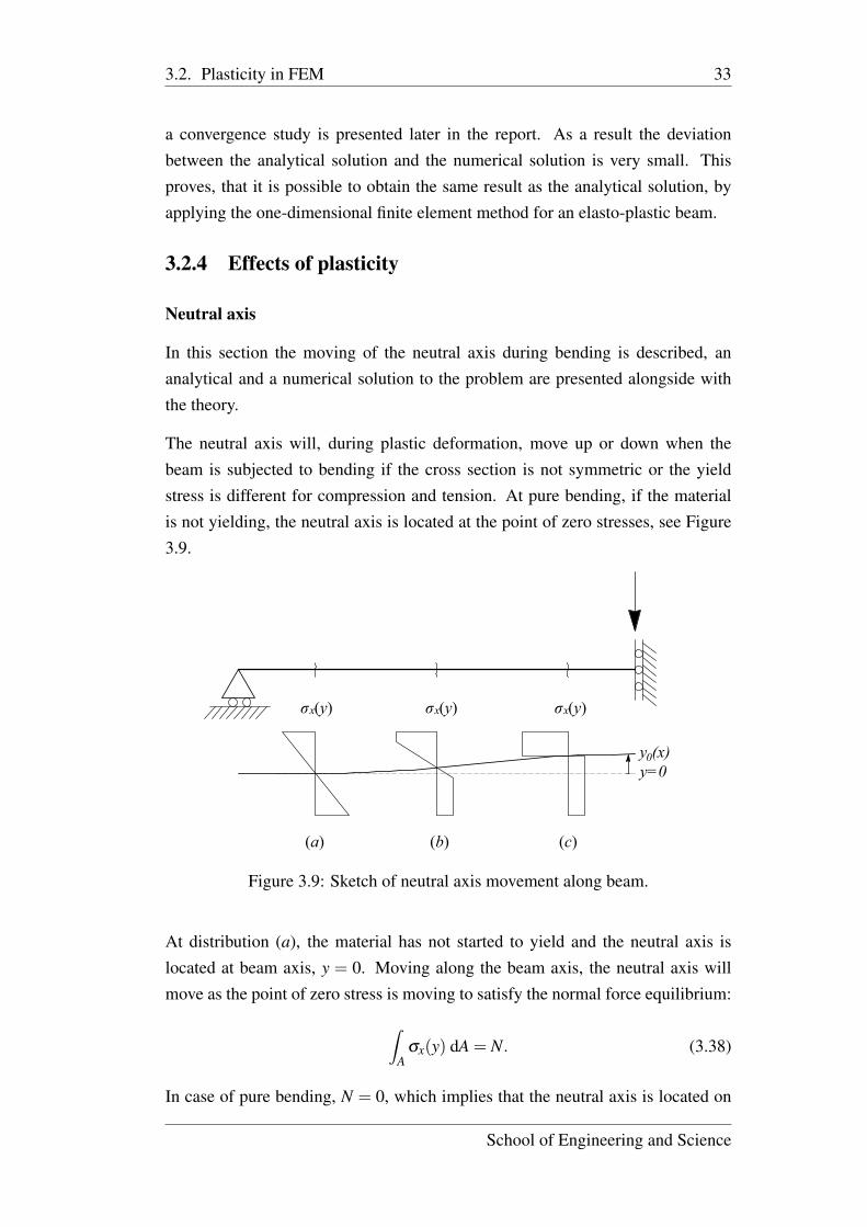
Neutral axis
In this section the moving of the neutral axis during bending is described, ananalytical and a numerical solution to the problem are presented alongside withthe theory.
The neutral axis will, during plastic deformation, move up or down when thebeam is subjected to bending if the cross section is not symmetric or the yieldstress is different for compression and tension. At pure bending, if the materialis not yielding, the neutral axis is located at the point of zero stresses, see Figure3.9.
y0(x)y=0
σx(y) σx(y)σx(y)
(b) (c) (a)
Figure 3.9: Sketch of neutral axis movement along beam.
At distribution (a), the material has not started to yield and the neutral axis islocated at beam axis, y = 0. Moving along the beam axis, the neutral axis willmove as the point of zero stress is moving to satisfy the normal force equilibrium:
∫A
σx(y) dA = N. (3.38)
In case of pure bending, N = 0, which implies that the neutral axis is located on
School of Engineering and Science

34 3.2. Plasticity in FEM
the beam axis. In Figure 3.9 it can be seen, that this is only true for elastic stressdistributions, as the neutral axis moves when yielding is reached (b).
If the coordinate system is kept unchanged during bending, a beam strain at theoriginal neutral axis may develop during yielding. The continuum strain in a crosssection can be described as stated in Equation (2.7).
During elastic bending the neutral axis is located at the centroid, which is calcu-lated as
Cy =
∫y f (y)dy∫f (y)dy
⇒ ∑ yAi
∑Ai. (3.39)
The y-axis is then defined as y = 0 = y−Cy, for y = 0 at the bottom of the profile.
For a cross section with a perfect elasto-plastic material that has the same strengthcharacteristics in compression and tension, the neutral axis in pure bending at fullplastic behaviour is located where the area above the neutral axis is equal to thearea below.
Calculating the location of the neutral axis, in-between elastic and fully plastic isa bit more difficult. One way of doing it is by iteration, where the out of balanceforce is converted to a strain and then added to the beam strain as
ε(i+1)0 =
−∫
A σxdA+N∫A E(y) dA
+ ε(i)0 . (3.40)
1. Initial position of the neutral axis is assumed located in the beam axis i.e.ε(1)0 = 0.
2. Normal stresses are calculated from εx(y) = ε(i)0 −κy.
3. Equation (3.40) is used to calculate a new ε(i+1)0 .
4. The iteration is converged when the out of balance force,∫
A σxdA−N, isnegligible small. If this is not the case, step 2-4 are repeated.
Analytical solution for a T-profile
The analytical solution to the location of the neutral axis depends on which partof the profile is yielding. A T-profile subjected to pure bending, the bottom partstarts yielding first if the material used is isotropic. The solution presented here isonly valid for yielding at the bottom of the profile, and with an isotropic perfectelasto-plastic material.
Aalborg University
3.2. Plasticity in FEM 35
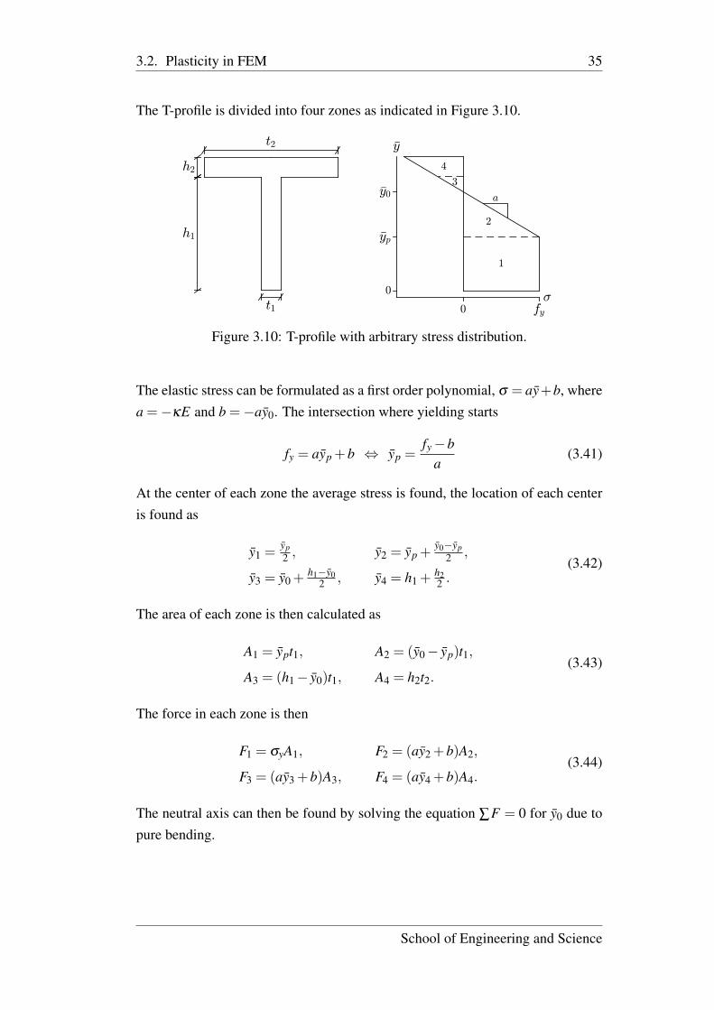
The T-profile is divided into four zones as indicated in Figure 3.10.
h1
h2
t1
t2
fy0<
0
7yp
7y0
7y
1
2
3
4
a
Figure 3.10: T-profile with arbitrary stress distribution.
The elastic stress can be formulated as a first order polynomial, σ = ay+b, wherea =−κE and b =−ay0. The intersection where yielding starts
fy = ayp +b ⇔ yp =fy−b
a(3.41)
At the center of each zone the average stress is found, the location of each centeris found as
y1 =yp2 , y2 = yp +
y0−yp2 ,
y3 = y0 +h1−y0
2 , y4 = h1 +h22 .
(3.42)
The area of each zone is then calculated as
A1 = ypt1, A2 = (y0− yp)t1,
A3 = (h1− y0)t1, A4 = h2t2.(3.43)
The force in each zone is then
F1 = σyA1, F2 = (ay2 +b)A2,
F3 = (ay3 +b)A3, F4 = (ay4 +b)A4.(3.44)
The neutral axis can then be found by solving the equation ∑F = 0 for y0 due topure bending.
School of Engineering and Science
36 3.2. Plasticity in FEM
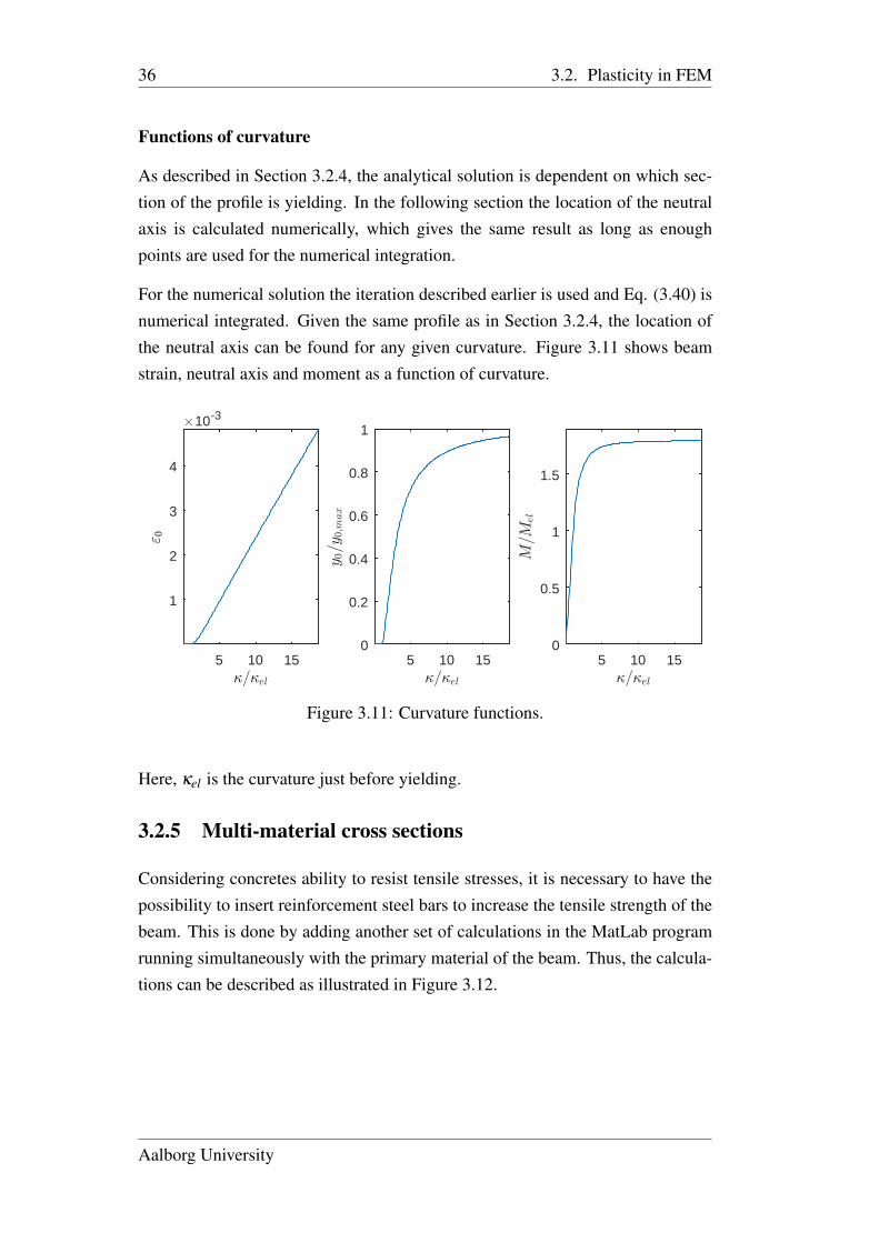
Functions of curvature
As described in Section 3.2.4, the analytical solution is dependent on which sec-tion of the profile is yielding. In the following section the location of the neutralaxis is calculated numerically, which gives the same result as long as enoughpoints are used for the numerical integration.
For the numerical solution the iteration described earlier is used and Eq. (3.40) isnumerical integrated. Given the same profile as in Section 3.2.4, the location ofthe neutral axis can be found for any given curvature. Figure 3.11 shows beamstrain, neutral axis and moment as a function of curvature.
5=5el
5 10 15
" 0
#10-3
1
2
3
4
5=5el
5 10 15
y 0=y
0;m
ax
0
0.2
0.4
0.6
0.8
1
5=5el
5 10 15
M=M
el
0
0.5
1
1.5
Figure 3.11: Curvature functions.
Here, κel is the curvature just before yielding.
3.2.5 Multi-material cross sections
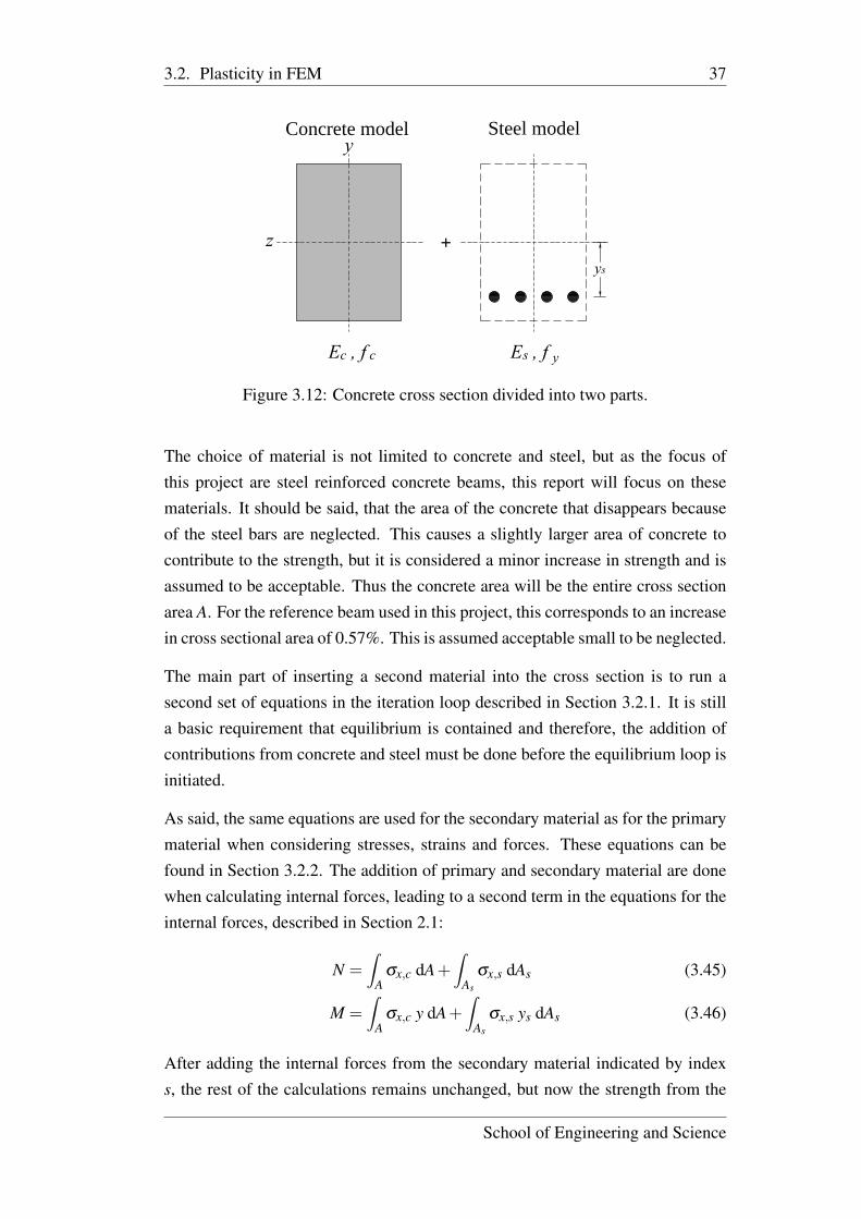
Considering concretes ability to resist tensile stresses, it is necessary to have thepossibility to insert reinforcement steel bars to increase the tensile strength of thebeam. This is done by adding another set of calculations in the MatLab programrunning simultaneously with the primary material of the beam. Thus, the calcula-tions can be described as illustrated in Figure 3.12.
Aalborg University
3.2. Plasticity in FEM 37
Concrete model
+
Steel model
Ec , f c Es , f y
z
y
ys
PR
OD
UC
ED
B
Y A
N A
UT
OD
ES
K E
DU
CA
TIO
NA
L P
RO
DU
CT
PRODUCED BY AN AUTODESK EDUCATIONAL PRODUCT
PR
OD
UC
ED
B
Y A
N A
UT
OD
ES
K E
DU
CA
TIO
NA
L P
RO
DU
CT
PRODUCED BY AN AUTODESK EDUCATIONAL PRODUCT
Figure 3.12: Concrete cross section divided into two parts.
The choice of material is not limited to concrete and steel, but as the focus ofthis project are steel reinforced concrete beams, this report will focus on thesematerials. It should be said, that the area of the concrete that disappears becauseof the steel bars are neglected. This causes a slightly larger area of concrete tocontribute to the strength, but it is considered a minor increase in strength and isassumed to be acceptable. Thus the concrete area will be the entire cross sectionarea A. For the reference beam used in this project, this corresponds to an increasein cross sectional area of 0.57%. This is assumed acceptable small to be neglected.
The main part of inserting a second material into the cross section is to run asecond set of equations in the iteration loop described in Section 3.2.1. It is stilla basic requirement that equilibrium is contained and therefore, the addition ofcontributions from concrete and steel must be done before the equilibrium loop isinitiated.
As said, the same equations are used for the secondary material as for the primarymaterial when considering stresses, strains and forces. These equations can befound in Section 3.2.2. The addition of primary and secondary material are donewhen calculating internal forces, leading to a second term in the equations for theinternal forces, described in Section 2.1:
N =∫
Aσx,c dA+
∫As
σx,s dAs (3.45)
M =∫
Aσx,c y dA+
∫As
σx,s ys dAs (3.46)
After adding the internal forces from the secondary material indicated by indexs, the rest of the calculations remains unchanged, but now the strength from the
School of Engineering and Science
38 3.3. Concrete material model
secondary material is included in the equilibrium loop, and the total strength willincrease. The increase in strength can be illustrated by observing a beam displace-ment progress. For the geometry, the benchmark values are used, see table1.1 (p.4).
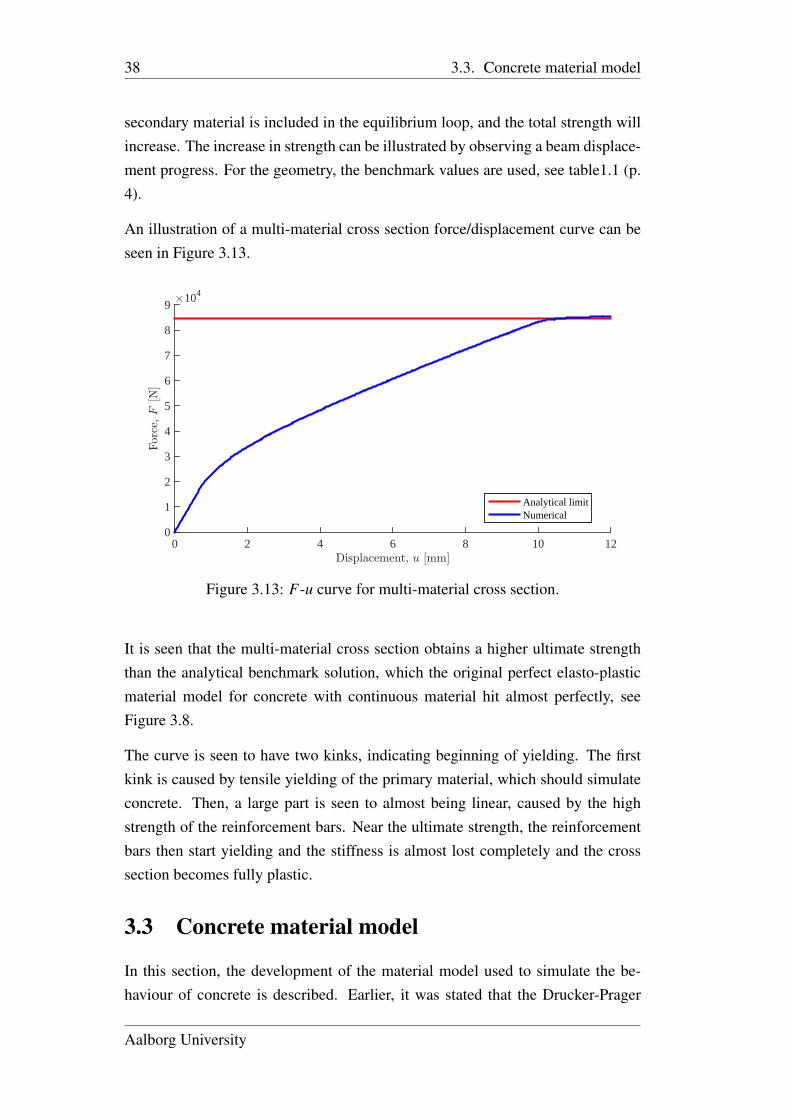
An illustration of a multi-material cross section force/displacement curve can beseen in Figure 3.13.
Displacement, u [mm]0 2 4 6 8 10 12
For
ce,F
[N]
#104
0
1
2
3
4
5
6
7
8
9
Analytical limitNumerical
Figure 3.13: F-u curve for multi-material cross section.
It is seen that the multi-material cross section obtains a higher ultimate strengththan the analytical benchmark solution, which the original perfect elasto-plasticmaterial model for concrete with continuous material hit almost perfectly, seeFigure 3.8.
The curve is seen to have two kinks, indicating beginning of yielding. The firstkink is caused by tensile yielding of the primary material, which should simulateconcrete. Then, a large part is seen to almost being linear, caused by the highstrength of the reinforcement bars. Near the ultimate strength, the reinforcementbars then start yielding and the stiffness is almost lost completely and the crosssection becomes fully plastic.
3.3 Concrete material model
In this section, the development of the material model used to simulate the be-haviour of concrete is described. Earlier, it was stated that the Drucker-Prager
Aalborg University
3.3. Concrete material model 39
criterion could be used to describe the behaviour. In this case, the yield criterioncan be simplified significantly, as the model is one-dimensional. The yield sur-face, described in Chapter 2, is boiled down to a "yield line" where the materialbecomes plastic when a yield point on the line is reached.
Earlier, the stress-strain curve for concrete was presented, see Chapter 1. Also,the use of linear elasto-plastic material model was presented in Chapter 2, whichdefined a point of yielding, where the material would go from linear elastic toperfect plastic.
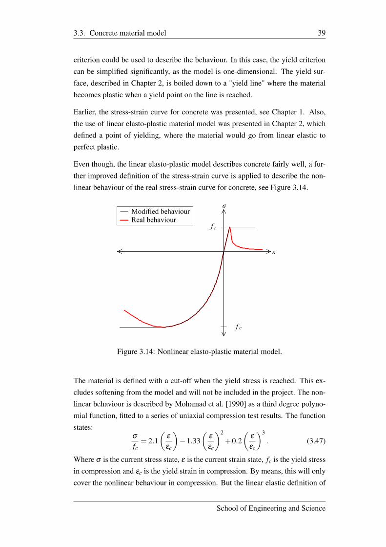
Even though, the linear elasto-plastic model describes concrete fairly well, a fur-ther improved definition of the stress-strain curve is applied to describe the non-linear behaviour of the real stress-strain curve for concrete, see Figure 3.14.
ε
σ
f c
f t
Modified behaviourReal behaviour
Figure 3.14: Nonlinear elasto-plastic material model.
The material is defined with a cut-off when the yield stress is reached. This ex-cludes softening from the model and will not be included in the project. The non-linear behaviour is described by Mohamad et al. [1990] as a third degree polyno-mial function, fitted to a series of uniaxial compression test results. The functionstates:
σ
fc= 2.1
(ε
εc
)−1.33
(ε
εc
)2
+0.2(
ε
εc
)3
. (3.47)
Where σ is the current stress state, ε is the current strain state, fc is the yield stressin compression and εc is the yield strain in compression. By means, this will onlycover the nonlinear behaviour in compression. But the linear elastic definition of
School of Engineering and Science
40 3.3. Concrete material model
the tensile behaviour is valid, so it is not necessary to improve further. The stressat a current state can now be found, only depending on the strain at this state.
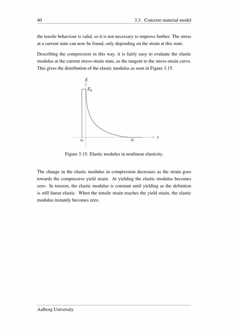
Describing the compression in this way, it is fairly easy to evaluate the elasticmodulus at the current stress-strain state, as the tangent to the stress-strain curve.This gives the distribution of the elastic modulus as seen in Figure 3.15.
ε
E
E0
εt εc
PR
OD
UC
ED
B
Y A
N A
UT
OD
ES
K E
DU
CA
TIO
NA
L P
RO
DU
CT
PRODUCED BY AN AUTODESK EDUCATIONAL PRODUCT
PR
OD
UC
ED
B
Y A
N A
UT
OD
ES
K E
DU
CA
TIO
NA
L P
RO
DU
CT
PRODUCED BY AN AUTODESK EDUCATIONAL PRODUCT
Figure 3.15: Elastic modulus in nonlinear elasticity.
The change in the elastic modulus in compression decreases as the strain goestowards the compressive yield strain. At yielding the elastic modulus becomeszero. In tension, the elastic modulus is constant until yielding as the definitionis still linear elastic. When the tensile strain reaches the yield strain, the elasticmodulus instantly becomes zero.
Aalborg University
41
Chapter 4
One-dimensional FE analysisIn this chapter, the beam model is analysed and a number of convergence analysisis performed. Also, the beam model will be compared to a model designed inAbaqus. The structure is a simply supported beam, subjected to a forced displace-ment at the center of the beam. The system and cross section data are describedin Chapter 1. Also, a concrete frame structure is analysed by using the MatLabscript to test the MatLab script with a more complex structure.
4.1 Element convergence
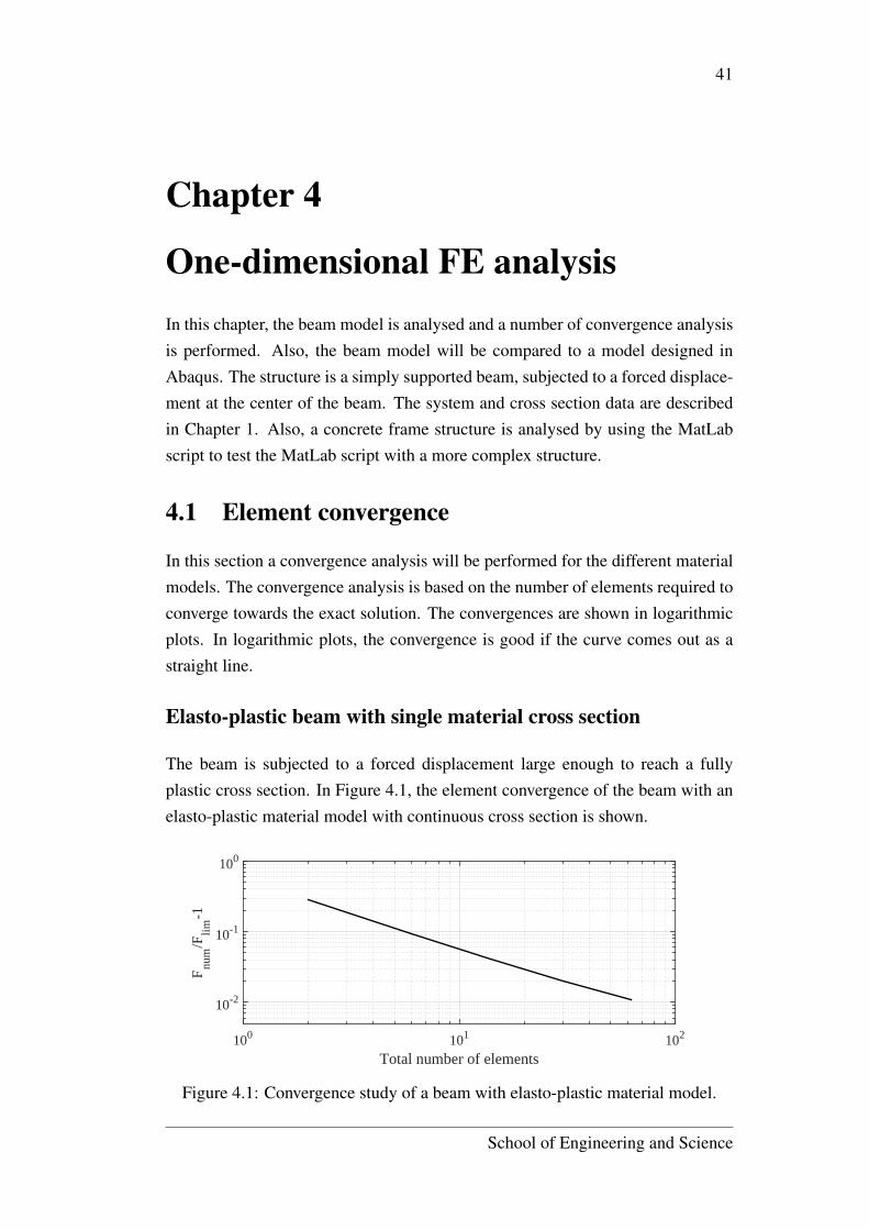
In this section a convergence analysis will be performed for the different materialmodels. The convergence analysis is based on the number of elements required toconverge towards the exact solution. The convergences are shown in logarithmicplots. In logarithmic plots, the convergence is good if the curve comes out as astraight line.
Elasto-plastic beam with single material cross section
The beam is subjected to a forced displacement large enough to reach a fullyplastic cross section. In Figure 4.1, the element convergence of the beam with anelasto-plastic material model with continuous cross section is shown.
Total number of elements100 101 102
Fnu
m/F
lim-1
10-2
10-1
100
Figure 4.1: Convergence study of a beam with elasto-plastic material model.
School of Engineering and Science
42 4.1. Element convergence
Here, the number of integration points over the cross section and number of crosssection integrations are kept constant to observe the effect of the total numberof elements only. The y axis shows the numerical value calculated, divided bythe analytical limit value minus one, which gives the error of numerical valuecompared to the analytical limit value. The line is almost completely straight,which means a good convergence.
To see what the gain in accuracy of using 60 elements rather than using 30 ele-ments, the error for 30 and 60 elements are given in Table 4.1.
Table 4.1: Convergence of elasto-plastic beam with continuous material crosssection.
No. elements Fnum Fnum/Flim-1 [%] Computational time [s]30 14.383×10⁵ N 2.0 6.3360 14.255×10⁵ N 1.1 12.92
Using 60 elements for the model will result in an error of 1.1%. Using 30 elementswill increase the error of 0.9%, but in return the computation time is reduced byhalf.
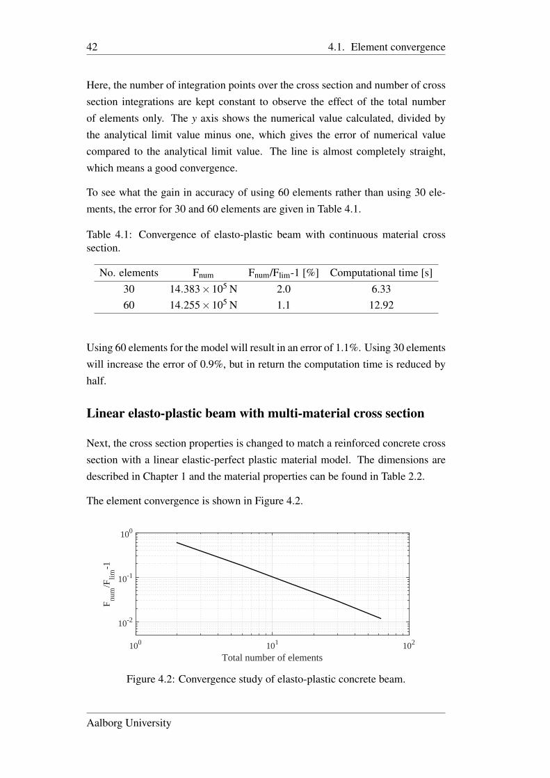
Linear elasto-plastic beam with multi-material cross section
Next, the cross section properties is changed to match a reinforced concrete crosssection with a linear elastic-perfect plastic material model. The dimensions aredescribed in Chapter 1 and the material properties can be found in Table 2.2.
The element convergence is shown in Figure 4.2.
Total number of elements100 101 102
Fnu
m/F
lim-1
10-2
10-1
100
Figure 4.2: Convergence study of elasto-plastic concrete beam.
Aalborg University
4.1. Element convergence 43
The convergence shows the same tendency as the elasto-plastic beam with a con-tinuous cross section. Again, use of 30 elements could be defended as the differ-ence is small. The convergence at 30 and 60 elements, are listed in Table 4.2.
Table 4.2: Convergence of elasto-plastic reinforced concrete beam.
No. elements Fnum Fnum/Flim-1 [%] Computational time [s]30 8.75×10⁴ N 2.99 7.7760 8.61×10⁴ N 1.27 14.54
The gain from using 60 elements in this case is greater than for the continuouscross section beam. The error is reduced with 1.72% by using 60 elements, butthe computational time is doubled up.
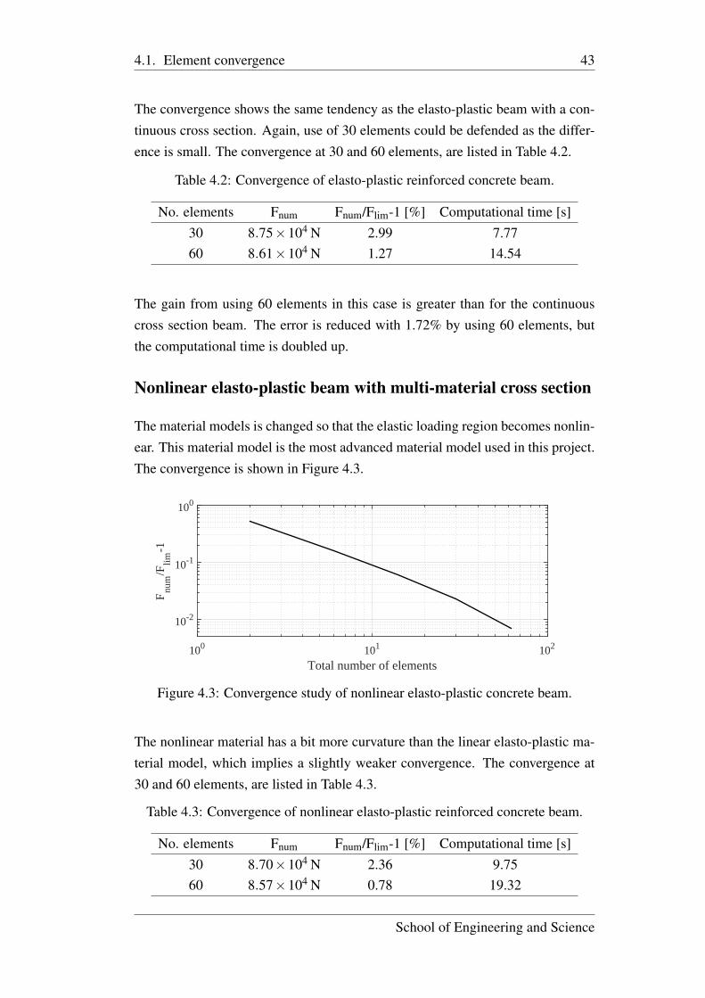
Nonlinear elasto-plastic beam with multi-material cross section
The material models is changed so that the elastic loading region becomes nonlin-ear. This material model is the most advanced material model used in this project.The convergence is shown in Figure 4.3.
Total number of elements100 101 102
Fnu
m/F
lim-1
10-2
10-1
100
Figure 4.3: Convergence study of nonlinear elasto-plastic concrete beam.
The nonlinear material has a bit more curvature than the linear elasto-plastic ma-terial model, which implies a slightly weaker convergence. The convergence at30 and 60 elements, are listed in Table 4.3.
Table 4.3: Convergence of nonlinear elasto-plastic reinforced concrete beam.
No. elements Fnum Fnum/Flim-1 [%] Computational time [s]30 8.70×10⁴ N 2.36 9.7560 8.57×10⁴ N 0.78 19.32
School of Engineering and Science
44 4.2. Elements versus integration points
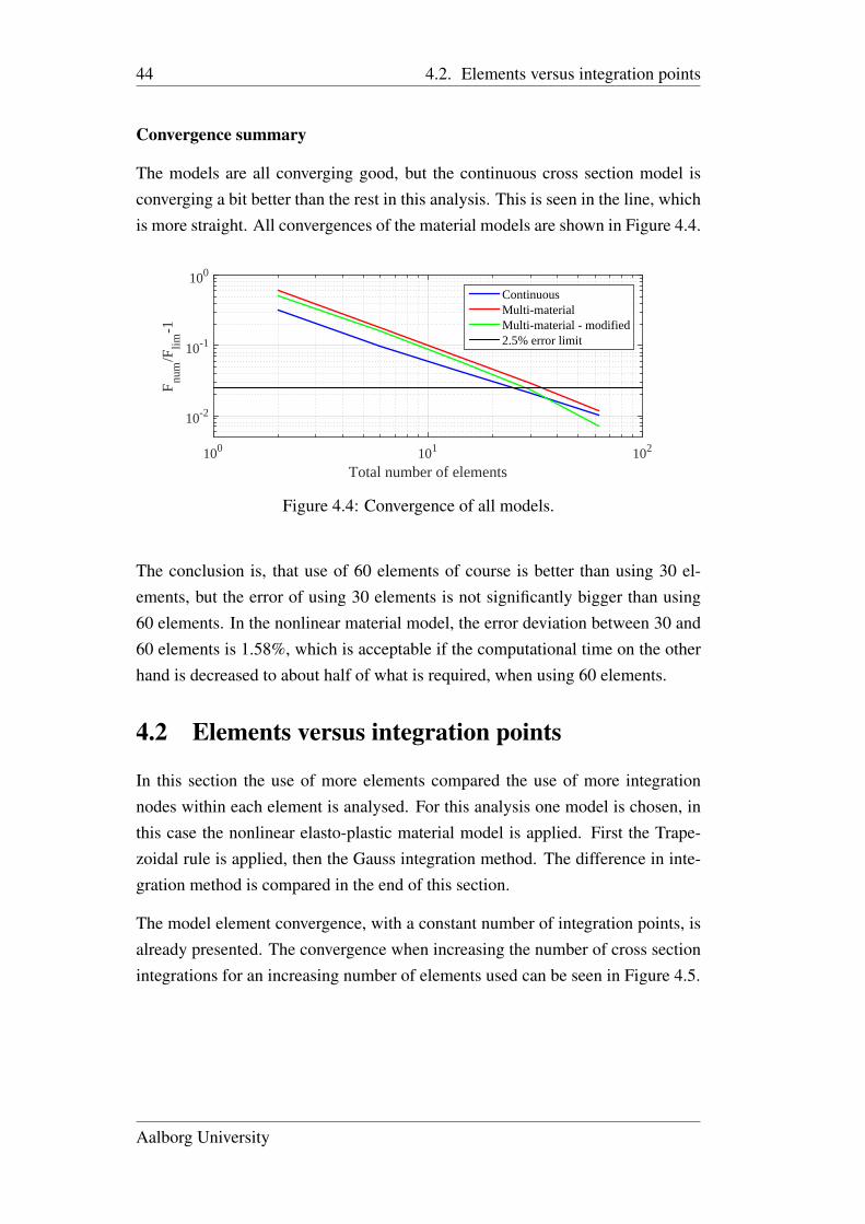
Convergence summary
The models are all converging good, but the continuous cross section model isconverging a bit better than the rest in this analysis. This is seen in the line, whichis more straight. All convergences of the material models are shown in Figure 4.4.
Total number of elements100 101 102
Fnu
m/F
lim-1
10-2
10-1
100
ContinuousMulti-materialMulti-material - modified2.5% error limit
Figure 4.4: Convergence of all models.
The conclusion is, that use of 60 elements of course is better than using 30 el-ements, but the error of using 30 elements is not significantly bigger than using60 elements. In the nonlinear material model, the error deviation between 30 and60 elements is 1.58%, which is acceptable if the computational time on the otherhand is decreased to about half of what is required, when using 60 elements.
4.2 Elements versus integration points
In this section the use of more elements compared the use of more integrationnodes within each element is analysed. For this analysis one model is chosen, inthis case the nonlinear elasto-plastic material model is applied. First the Trape-zoidal rule is applied, then the Gauss integration method. The difference in inte-gration method is compared in the end of this section.
The model element convergence, with a constant number of integration points, isalready presented. The convergence when increasing the number of cross sectionintegrations for an increasing number of elements used can be seen in Figure 4.5.
Aalborg University
4.2. Elements versus integration points 45
Total cross section integrations101 102 103
Fnu
m/F
lim-1
10-2
10-1
100
2 elements6 elements14 elements30 elements62 elements
Figure 4.5: Integration points over beam length - Trapezoidal rule.
In Figure 4.6 the number of integration points over the cross section height varytogether with the number of elements.
Cross section integration points10 20 30 40 50 60
Fnu
m/F
lim-1
10-2
10-1
100
2 elements6 elements14 elements30 elements62 elements
Figure 4.6: Integration points over cross section height - Trapezoidal rule.
It is seen, that the number of cross section integrations only influence the con-vergence when using 2 elements. When the number of elements is increased, theimportance of the number of elements is greater than the number of cross sectionintegrations and there is no further gain from using more cross section integra-tions.
Observing the number of integration points over the cross section height, the op-posite tendency is seen. Here, the number of integration points is more importantwhen the number of elements is increasing.
Now the integration method is changed to Gauss integration. First, the analysis iscarried out for the total number of cross section integrations. The results is shownin Figure 4.7
School of Engineering and Science
46 4.2. Elements versus integration points
Total cross section intetrations101 102 103
Fnu
m/F
lim-1
10-2
10-1
100
2 elements6 elements14 elements30 elements62 elements
Figure 4.7: Integration points over beam length - Gauss integration.
The convergence study shows even less influence from the number of cross sectionintegrations, when the Gauss quadrature is applied. This shows, that the Gaussquadrature might be better fitted to use when considering the integration overlength.
The analysis is now carried out for the integration points over the beam crosssection height. The results is shown in Figure 4.8
Cross section integration points10 20 30 40 50 60
Fnu
m/F
lim-1
10-2
10-1
100
2 elements6 elements14 elements30 elements62 elements
Figure 4.8: Integration points over cross section height - Gauss integration.
Here, the same tendency as for the trapezoidal rule. The more elements used, themore influence the number of integration points over the cross section height has.Gauss integration seems to be a worse fit for the integration over the cross sectionheight as the convergence lines has irregularities when more elements are used.
When observing the influence of the integration method, it could be interesting toobserve the stress distribution over the cross section height. At the point of firstyield, the plastic strains will occur at the top or bottom of the beam first. As the
Aalborg University
4.3. Iteration scheme methods 47
difference between the trapezoidal rule and Gauss integration is the location ofthe integration points near the edges, a change might be found in the distributionof stresses.
In Figure 4.9 and Figure 4.10, the stress distribution for the beam at some pointof loading are shown.
-100 0 1000
50
100
150
200
250
300
Normal stress [MPa]-30 -20 -10 0
y[m
m]
-100
-50
0
50
100
150
#10-3
0 2
-100
-50
0
50
100
150
Figure 4.9: Stress distribution withtrapezoidal rule over cross sectionheight.
-100 0 1000
50
100
150
200
250
300
Normal stress [MPa]-30 -20 -10 0
y[m
m]
-100
-50
0
50
100
150
#10-3
0 2
-100
-50
0
50
100
150
Figure 4.10: Stress distribution withgauss integration over cross sectionheight.
It is seen, that the gauss integration points are suited better when observing yield-ing at the edge. But, the trapezoidal rule is more accurate in the middle of thecross section. The difference is so small, that the choice of integration method isunimportant. The choice may therefore be the trapezoidal rule, as the convergencestudy showed this to be better suited for cross section integration.
4.3 Iteration scheme methods
The iteration schemes should not cause any difference in the convergence. But,an improved iteration scheme could decrease the computational time. In thisanalysis, the modified Newton-Raphson scheme is compared to the full Newton-Raphson scheme. The difference is as described earlier, that the modified Newton-Raphson only updates the stiffness for every load increment, where the full Newton-Raphson scheme updates the stiffness for every iteration. In this comparison, theinteresting parameters are total number of iterations used and computational time
School of Engineering and Science
48 4.4. Concrete beam analysis
used on calculations. The analysis is done for a fully converged model loaded toa fully plastic cross section. The results can be found in Table 4.4.
Table 4.4: Iteration scheme comparison.
Total number of iterations Elapsed timeModified Newton-Raphson 302 20.6 sFull Newton-Raphson 64 6.2 s
The results shows a significant reduction in both amount of iterations needed andin computational time. The update of the stiffness is very beneficial, and thecomputational time of setting up the stiffness matrix for each iteration is muchfaster than iterating to the correct value with an initial stiffness of the given loadincrement.
Summary
From previous analysis, regarding the different calculation methods used in theMatLab program, it can be concluded that the convergence is highly dependingon the number of elements used, not only is this the most contributing factor tothe convergence, but the integration over height and length is also depending onthe number of elements. The choice of scheme method only have influence onthe calculation time. Here, the full Newton-Raphson was the fastest and mosteffective.
4.4 Concrete beam analysis
In this section, a beam subjected to a forced displacement is analysed. As saidearlier, the results will be compared to other solutions from different methods andprograms. For the material model, the nonlinear elasto-plastic material model isapplied. This is the most advanced and accurate material model for concrete usedin this project and will give the best results for concrete structures. The beamdimensions are given in Table 4.5.
Aalborg University
4.4. Concrete beam analysis 49
Table 4.5: Concrete beam properties.
GeometryCross section 300 mm×200 mmLength 3000 mmRebars 3×12 mmRebar distance from bottom 50 mmConcreteYield stress ( ft/ fc) 3 MPa/30 MPaInitial Young’s modulus 30×103 MPaReinforcement steelYield stress ( fy) 550 MPaYoung’s modulus 210×103 MPa
Modelling
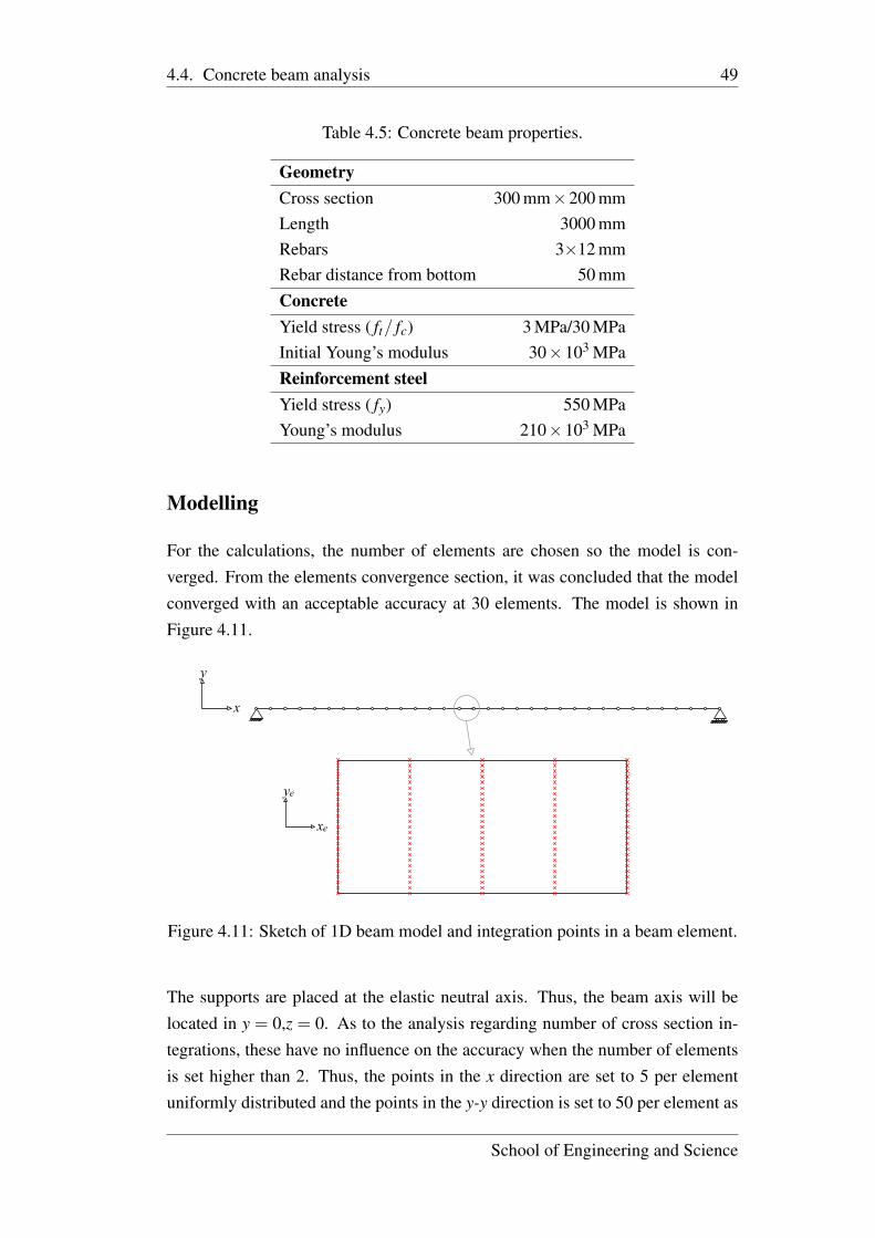
For the calculations, the number of elements are chosen so the model is con-verged. From the elements convergence section, it was concluded that the modelconverged with an acceptable accuracy at 30 elements. The model is shown inFigure 4.11.
xe
ye
x
y
Figure 4.11: Sketch of 1D beam model and integration points in a beam element.
The supports are placed at the elastic neutral axis. Thus, the beam axis will belocated in y = 0,z = 0. As to the analysis regarding number of cross section in-tegrations, these have no influence on the accuracy when the number of elementsis set higher than 2. Thus, the points in the x direction are set to 5 per elementuniformly distributed and the points in the y-y direction is set to 50 per element as
School of Engineering and Science
50 4.4. Concrete beam analysis
the number of elements used requires that the number of integration points overthe cross section height is set this high. The beam element can be seen in Figure4.11.
The forced displacement is done at the center of the beam at the beam axis. Themaximum displacement is set to 20 mm. Here the cross section becomes fullyplastic.
Results
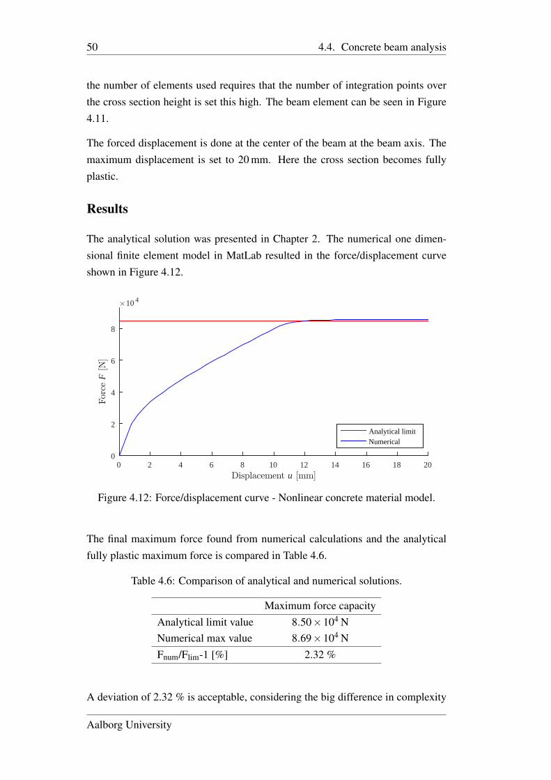
The analytical solution was presented in Chapter 2. The numerical one dimen-sional finite element model in MatLab resulted in the force/displacement curveshown in Figure 4.12.
Displacement u [mm]0 2 4 6 8 10 12 14 16 18 20
For
ceF
[N]
#10 4
0
2
4
6
8
Analytical limitNumerical
Figure 4.12: Force/displacement curve - Nonlinear concrete material model.
The final maximum force found from numerical calculations and the analyticalfully plastic maximum force is compared in Table 4.6.
Table 4.6: Comparison of analytical and numerical solutions.
Maximum force capacityAnalytical limit value 8.50×10⁴ NNumerical max value 8.69×10⁴ NFnum/Flim-1 [%] 2.32 %
A deviation of 2.32 % is acceptable, considering the big difference in complexity
Aalborg University
4.4. Concrete beam analysis 51
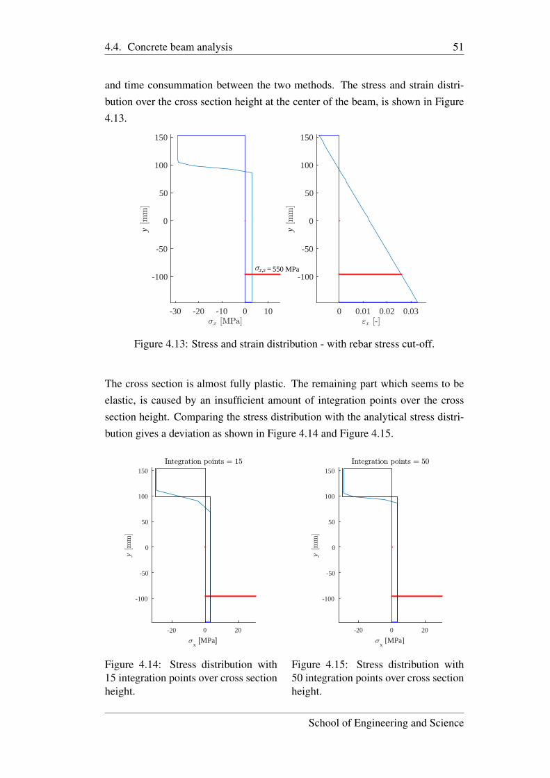
and time consummation between the two methods. The stress and strain distri-bution over the cross section height at the center of the beam, is shown in Figure4.13.
-100 -50 0 50 100-150
-100
50
0
-50
100
150
<x [MPa]-30 -20 -10 0 10
y[m
m]
-100
-50
0
50
100
150
"x [-]0 0.01 0.02 0.03
y[m
m]
-100
-50
0
50
100
150
= 550 MPax< ,s
Figure 4.13: Stress and strain distribution - with rebar stress cut-off.
The cross section is almost fully plastic. The remaining part which seems to beelastic, is caused by an insufficient amount of integration points over the crosssection height. Comparing the stress distribution with the analytical stress distri-bution gives a deviation as shown in Figure 4.14 and Figure 4.15.
Cross Section
<x [MPa]
-20 0 20
y[m
m]
-100
-50
0
50
100
150
Integration points = 15
0x [-]
0 0.02 0.04
y[m
m]
-100
-50
0
50
100
150Strain distribution
Figure 4.14: Stress distribution with15 integration points over cross sectionheight.
Cross Section
<x [MPa]
-20 0 20
y[m
m]
-100
-50
0
50
100
150
Integration points = 50
0x [-]
-0.01 0 0.01 0.02 0.03
y[m
m]
-100
-50
0
50
100
150Strain distribution
Figure 4.15: Stress distribution with50 integration points over cross sectionheight.
School of Engineering and Science
52 4.4. Concrete beam analysis
The black line indicates the analytical stress distribution. It is observed that thenumerical model deviates from the exact solution, but goes towards the exact so-lution when more integration points are used to distribute the stresses over thecross section height.
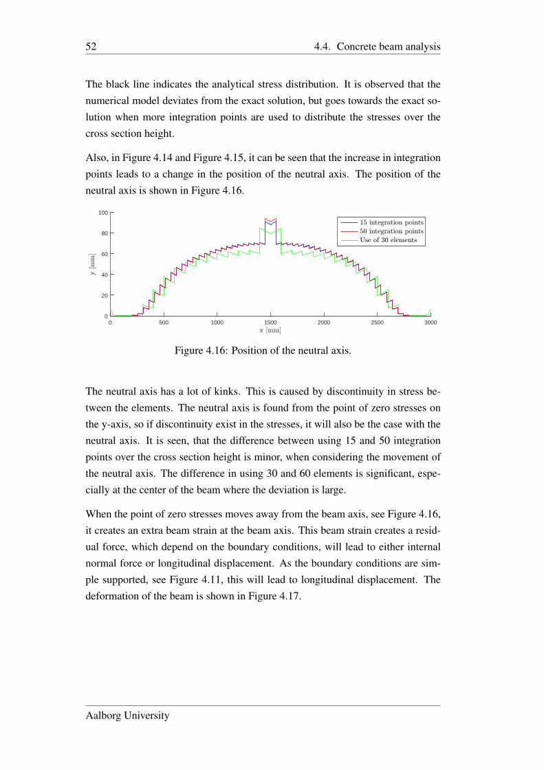
Also, in Figure 4.14 and Figure 4.15, it can be seen that the increase in integrationpoints leads to a change in the position of the neutral axis. The position of theneutral axis is shown in Figure 4.16.
x [mm]0 500 1000 1500 2000 2500 3000
y[m
m]
0
20
40
60
80
100
15 integration points
50 integration points
Use of 30 elements
Figure 4.16: Position of the neutral axis.
The neutral axis has a lot of kinks. This is caused by discontinuity in stress be-tween the elements. The neutral axis is found from the point of zero stresses onthe y-axis, so if discontinuity exist in the stresses, it will also be the case with theneutral axis. It is seen, that the difference between using 15 and 50 integrationpoints over the cross section height is minor, when considering the movement ofthe neutral axis. The difference in using 30 and 60 elements is significant, espe-cially at the center of the beam where the deviation is large.
When the point of zero stresses moves away from the beam axis, see Figure 4.16,it creates an extra beam strain at the beam axis. This beam strain creates a resid-ual force, which depend on the boundary conditions, will lead to either internalnormal force or longitudinal displacement. As the boundary conditions are sim-ple supported, see Figure 4.11, this will lead to longitudinal displacement. Thedeformation of the beam is shown in Figure 4.17.
Aalborg University
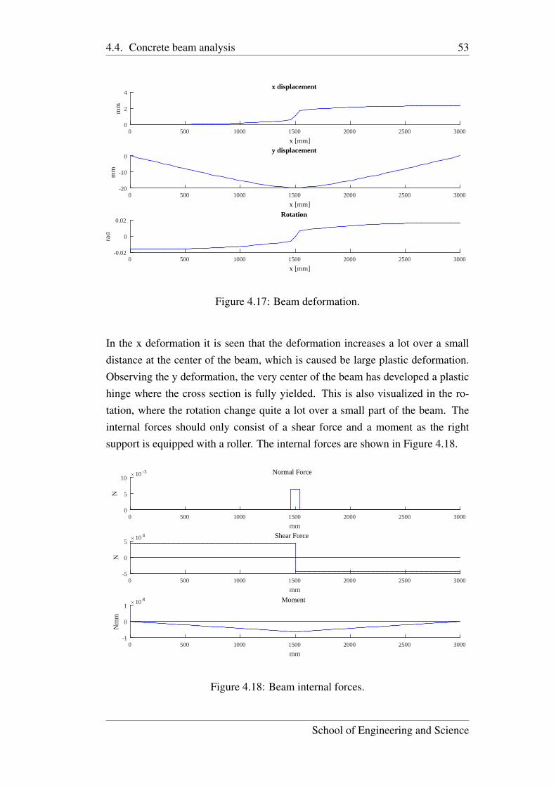
4.4. Concrete beam analysis 53
x [mm]0 500 1000 1500 2000 2500 3000
mm
0
2
4x displacement
x [mm]0 500 1000 1500 2000 2500 3000
mm
-20
-10
0y displacement
x [mm]0 500 1000 1500 2000 2500 3000
rad
-0.02
0
0.02Rotation
Figure 4.17: Beam deformation.
In the x deformation it is seen that the deformation increases a lot over a smalldistance at the center of the beam, which is caused be large plastic deformation.Observing the y deformation, the very center of the beam has developed a plastichinge where the cross section is fully yielded. This is also visualized in the ro-tation, where the rotation change quite a lot over a small part of the beam. Theinternal forces should only consist of a shear force and a moment as the rightsupport is equipped with a roller. The internal forces are shown in Figure 4.18.
mm0 500 1000 1500 2000 2500 3000
N
#10 -3
0
5
10Normal Force
mm0 500 1000 1500 2000 2500 3000
N
#10 4
-5
0
5Shear Force
mm0 500 1000 1500 2000 2500 3000
Nm
m
#10 8
-1
0
1Moment
Figure 4.18: Beam internal forces.
School of Engineering and Science
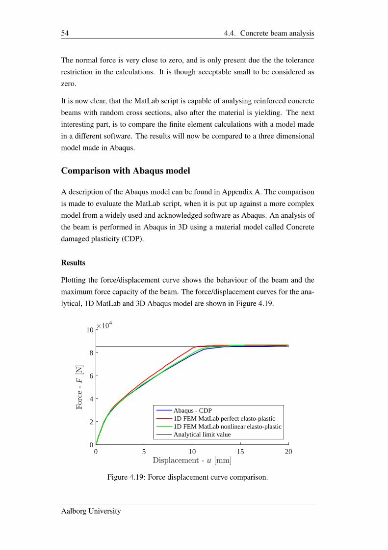
54 4.4. Concrete beam analysis
The normal force is very close to zero, and is only present due the the tolerancerestriction in the calculations. It is though acceptable small to be considered aszero.
It is now clear, that the MatLab script is capable of analysing reinforced concretebeams with random cross sections, also after the material is yielding. The nextinteresting part, is to compare the finite element calculations with a model madein a different software. The results will now be compared to a three dimensionalmodel made in Abaqus.
Comparison with Abaqus model
A description of the Abaqus model can be found in Appendix A. The comparisonis made to evaluate the MatLab script, when it is put up against a more complexmodel from a widely used and acknowledged software as Abaqus. An analysis ofthe beam is performed in Abaqus in 3D using a material model called Concretedamaged plasticity (CDP).
Results
Plotting the force/displacement curve shows the behaviour of the beam and themaximum force capacity of the beam. The force/displacement curves for the ana-lytical, 1D MatLab and 3D Abaqus model are shown in Figure 4.19.
Displacement - u [mm]0 5 10 15 20
For
ce-
F[N
]
#104
0
2
4
6
8
10
Abaqus - CDP1D FEM MatLab perfect elasto-plastic1D FEM MatLab nonlinear elasto-plasticAnalytical limit value
Figure 4.19: Force displacement curve comparison.
Aalborg University
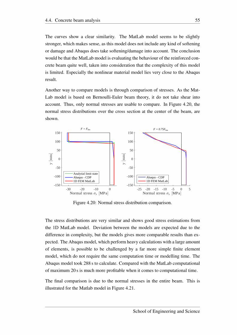
4.4. Concrete beam analysis 55
The curves show a clear similarity. The MatLab model seems to be slightlystronger, which makes sense, as this model does not include any kind of softeningor damage and Abaqus does take softening/damage into account. The conclusionwould be that the MatLab model is evaluating the behaviour of the reinforced con-crete beam quite well, taken into consideration that the complexity of this modelis limited. Especially the nonlinear material model lies very close to the Abaqusresult.
Another way to compare models is through comparison of stresses. As the Mat-Lab model is based on Bernoulli-Euler beam theory, it do not take shear intoaccount. Thus, only normal stresses are usable to compare. In Figure 4.20, thenormal stress distributions over the cross section at the center of the beam, areshown.
Normal st ress <x [MPa]-30 -20 -10 0
y[ m
m]
-150
-100
-50
0
50
100
150
Analytial limit stateAbaqus - CDP1D FEM MatLab
Normal st ress <x [MPa]-25 -20 -15 -10 -5 0 5
y[m
m]
-150
-100
-50
0
50
100
150
Abaqus - CDP1D FEM MatLab
F = Flim limF = 0.75F
Figure 4.20: Normal stress distribution comparison.
The stress distributions are very similar and shows good stress estimations fromthe 1D MatLab model. Deviation between the models are expected due to thedifference in complexity, but the models gives more comparable results than ex-pected. The Abaqus model, which perform heavy calculations with a large amountof elements, is possible to be challenged by a far more simple finite elementmodel, which do not require the same computation time or modelling time. TheAbaqus model took 288 s to calculate. Compared with the MatLab computationalof maximum 20 s is much more profitable when it comes to computational time.
The final comparison is due to the normal stresses in the entire beam. This isillustrated for the Matlab model in Figure 4.21.
School of Engineering and Science
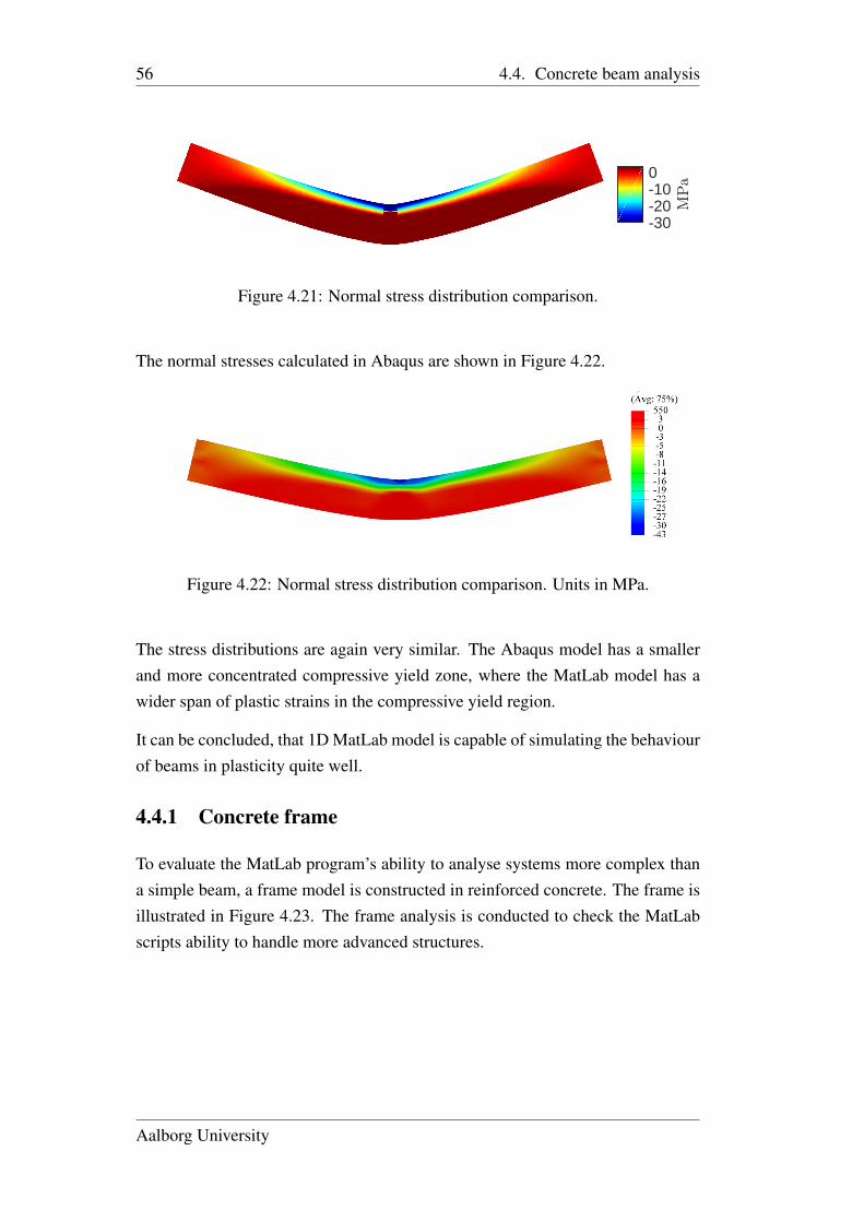
56 4.4. Concrete beam analysis
MPa
-30-20-100
Figure 4.21: Normal stress distribution comparison.
The normal stresses calculated in Abaqus are shown in Figure 4.22.
Printed using Abaqus/CAE on: Fri Jun 03 11:12:59 Romance Daylight Time 2016
Figure 4.22: Normal stress distribution comparison. Units in MPa.
The stress distributions are again very similar. The Abaqus model has a smallerand more concentrated compressive yield zone, where the MatLab model has awider span of plastic strains in the compressive yield region.
It can be concluded, that 1D MatLab model is capable of simulating the behaviourof beams in plasticity quite well.
4.4.1 Concrete frame
To evaluate the MatLab program’s ability to analyse systems more complex thana simple beam, a frame model is constructed in reinforced concrete. The frame isillustrated in Figure 4.23. The frame analysis is conducted to check the MatLabscripts ability to handle more advanced structures.
Aalborg University
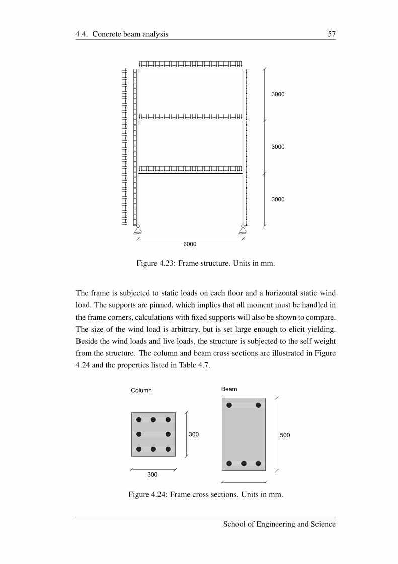
4.4. Concrete beam analysis 57
3000
3000
3000
6000
Figure 4.23: Frame structure. Units in mm.
The frame is subjected to static loads on each floor and a horizontal static windload. The supports are pinned, which implies that all moment must be handled inthe frame corners, calculations with fixed supports will also be shown to compare.The size of the wind load is arbitrary, but is set large enough to elicit yielding.Beside the wind loads and live loads, the structure is subjected to the self weightfrom the structure. The column and beam cross sections are illustrated in Figure4.24 and the properties listed in Table 4.7.
Column
Beam
300
300
500
6000
300
Figure 4.24: Frame cross sections. Units in mm.
School of Engineering and Science
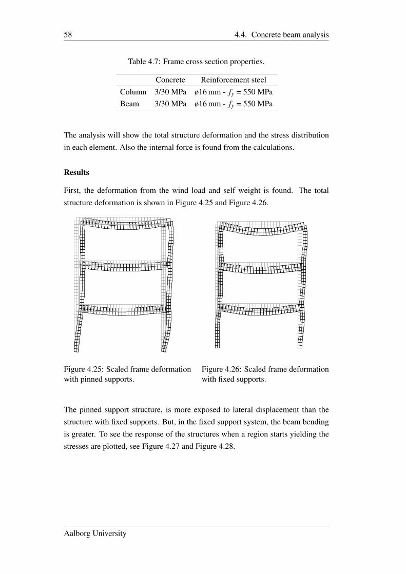
58 4.4. Concrete beam analysis
Table 4.7: Frame cross section properties.
Concrete Reinforcement steelColumn 3/30 MPa ø16 mm - fy = 550 MPaBeam 3/30 MPa ø16 mm - fy = 550 MPa
The analysis will show the total structure deformation and the stress distributionin each element. Also the internal force is found from the calculations.
Results
First, the deformation from the wind load and self weight is found. The totalstructure deformation is shown in Figure 4.25 and Figure 4.26.
Figure 4.25: Scaled frame deformationwith pinned supports.
Figure 4.26: Scaled frame deformationwith fixed supports.
The pinned support structure, is more exposed to lateral displacement than thestructure with fixed supports. But, in the fixed support system, the beam bendingis greater. To see the response of the structures when a region starts yielding thestresses are plotted, see Figure 4.27 and Figure 4.28.
Aalborg University
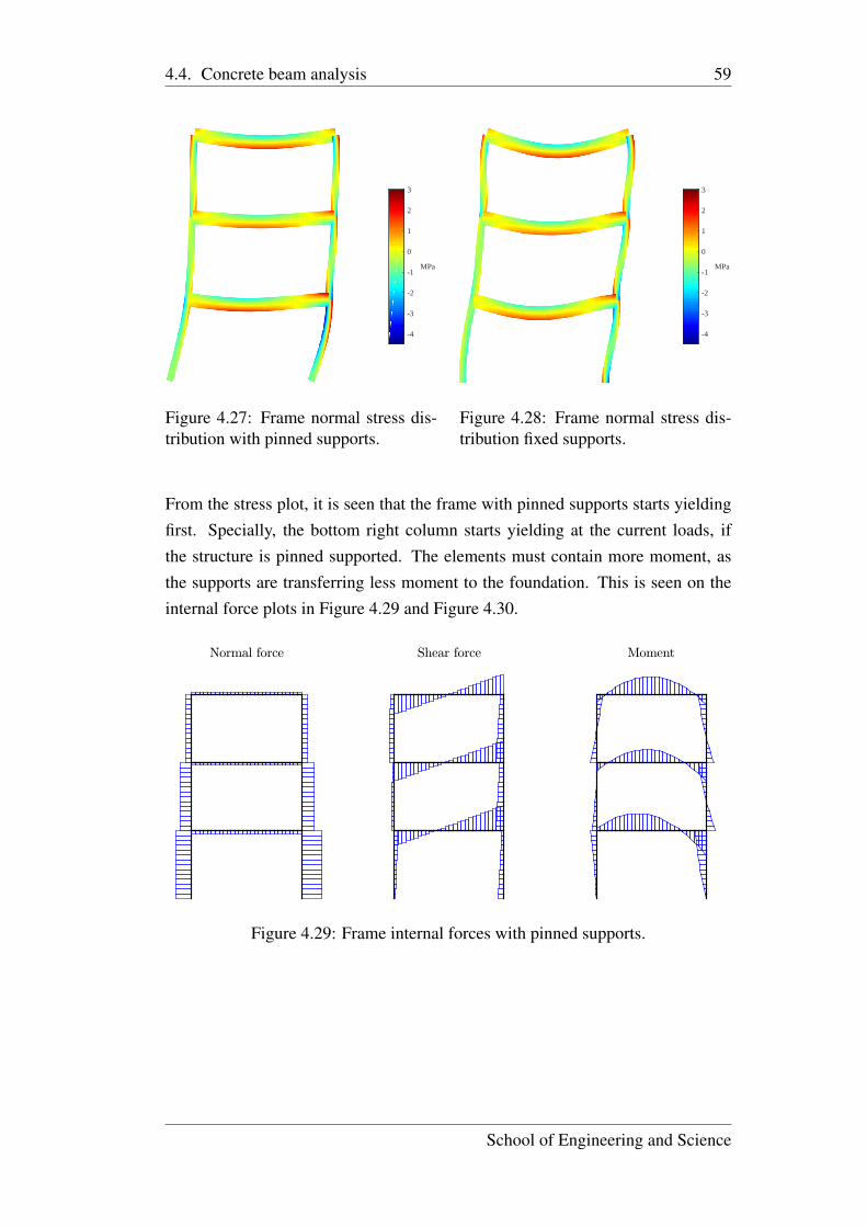
4.4. Concrete beam analysis 59
MPa
-4
-3
-2
-1
0
1
2
3
Figure 4.27: Frame normal stress dis-tribution with pinned supports.
MPa
-4
-3
-2
-1
0
1
2
3
Figure 4.28: Frame normal stress dis-tribution fixed supports.
From the stress plot, it is seen that the frame with pinned supports starts yieldingfirst. Specially, the bottom right column starts yielding at the current loads, ifthe structure is pinned supported. The elements must contain more moment, asthe supports are transferring less moment to the foundation. This is seen on theinternal force plots in Figure 4.29 and Figure 4.30.
Normal force Shear force Moment
Figure 4.29: Frame internal forces with pinned supports.
School of Engineering and Science
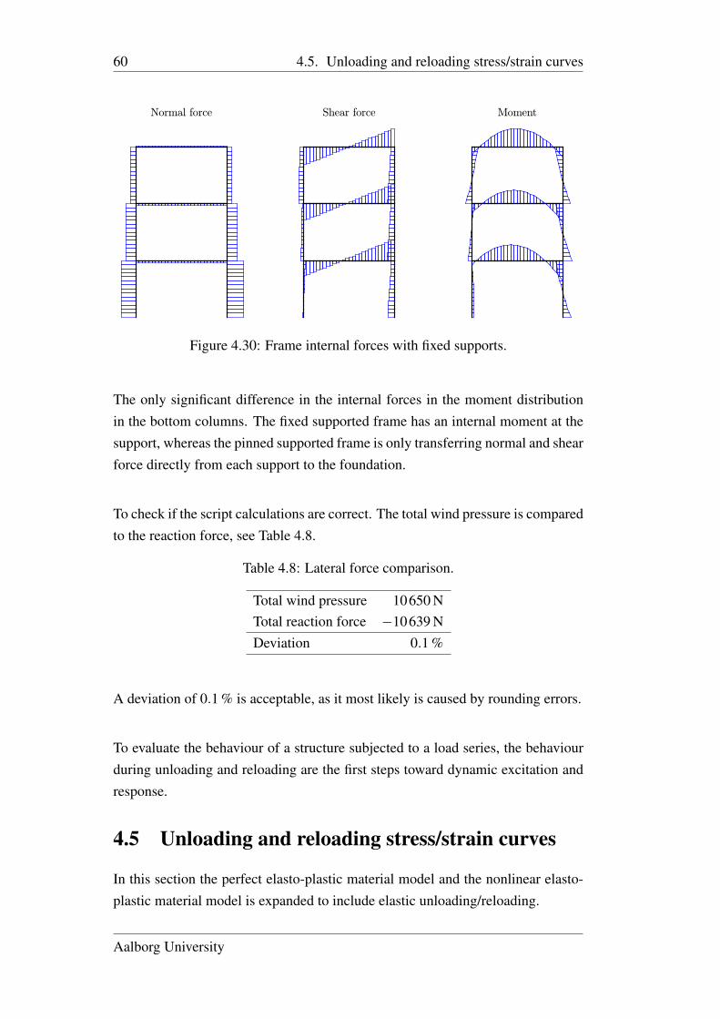
60 4.5. Unloading and reloading stress/strain curves
Normal force Shear force Moment
Figure 4.30: Frame internal forces with fixed supports.
The only significant difference in the internal forces in the moment distributionin the bottom columns. The fixed supported frame has an internal moment at thesupport, whereas the pinned supported frame is only transferring normal and shearforce directly from each support to the foundation.
To check if the script calculations are correct. The total wind pressure is comparedto the reaction force, see Table 4.8.
Table 4.8: Lateral force comparison.
Total wind pressure 10650 NTotal reaction force −10639 NDeviation 0.1 %
A deviation of 0.1 % is acceptable, as it most likely is caused by rounding errors.
To evaluate the behaviour of a structure subjected to a load series, the behaviourduring unloading and reloading are the first steps toward dynamic excitation andresponse.
4.5 Unloading and reloading stress/strain curves
In this section the perfect elasto-plastic material model and the nonlinear elasto-plastic material model is expanded to include elastic unloading/reloading.
Aalborg University
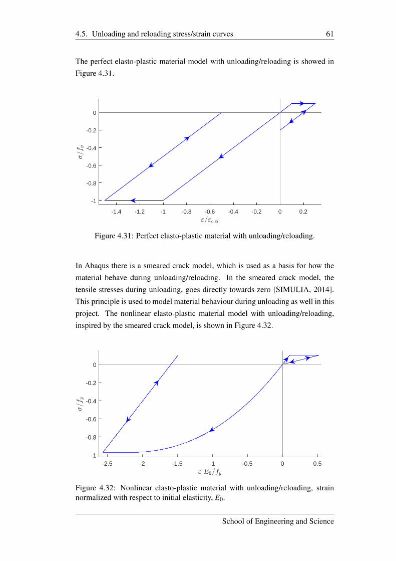
4.5. Unloading and reloading stress/strain curves 61
The perfect elasto-plastic material model with unloading/reloading is showed inFigure 4.31.
"="c;el
-1.4 -1.2 -1 -0.8 -0.6 -0.4 -0.2 0 0.2
<=f y
-1
-0.8
-0.6
-0.4
-0.2
0
Figure 4.31: Perfect elasto-plastic material with unloading/reloading.
In Abaqus there is a smeared crack model, which is used as a basis for how thematerial behave during unloading/reloading. In the smeared crack model, thetensile stresses during unloading, goes directly towards zero [SIMULIA, 2014].This principle is used to model material behaviour during unloading as well in thisproject. The nonlinear elasto-plastic material model with unloading/reloading,inspired by the smeared crack model, is shown in Figure 4.32.
" E0=fy
-2.5 -2 -1.5 -1 -0.5 0 0.5
<=f
y
-1
-0.8
-0.6
-0.4
-0.2
0
Figure 4.32: Nonlinear elasto-plastic material with unloading/reloading, strainnormalized with respect to initial elasticity, E0.
School of Engineering and Science
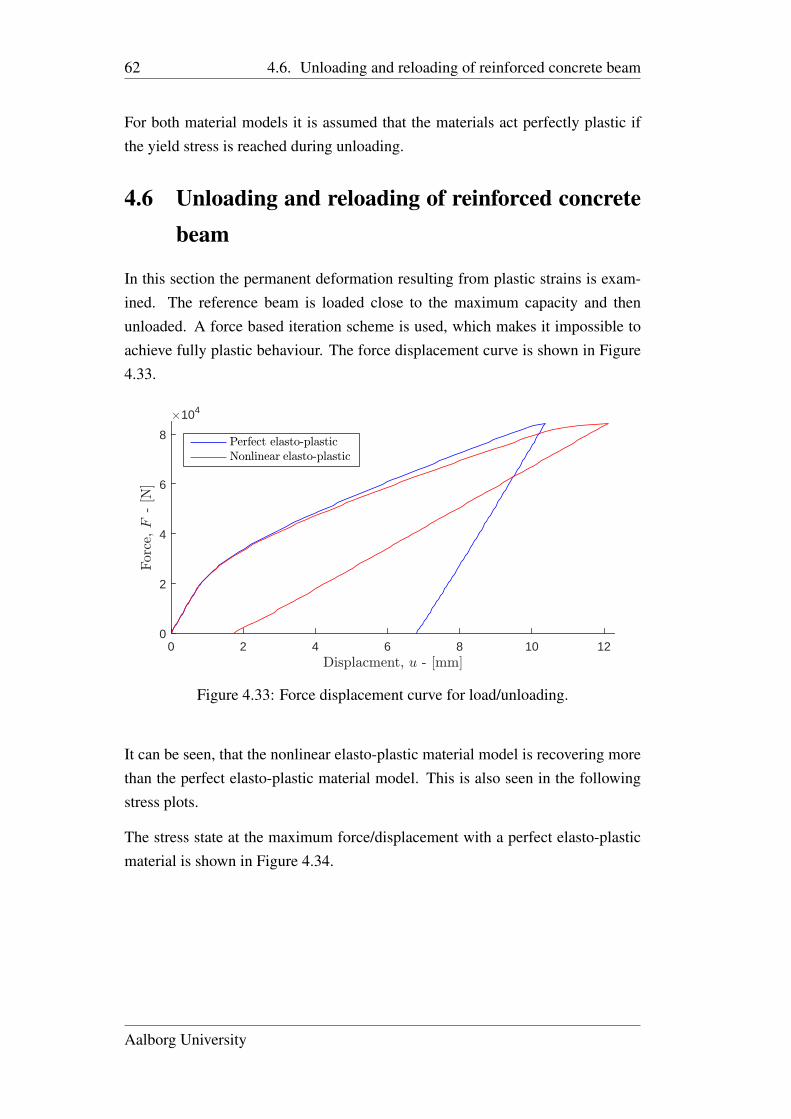
62 4.6. Unloading and reloading of reinforced concrete beam
For both material models it is assumed that the materials act perfectly plastic ifthe yield stress is reached during unloading.
4.6 Unloading and reloading of reinforced concretebeam
In this section the permanent deformation resulting from plastic strains is exam-ined. The reference beam is loaded close to the maximum capacity and thenunloaded. A force based iteration scheme is used, which makes it impossible toachieve fully plastic behaviour. The force displacement curve is shown in Figure4.33.
Displacment, u - [mm]0 2 4 6 8 10 12
For
ce,F
-[N
]
#104
0
2
4
6
8Perfect elasto-plastic Nonlinear elasto-plastic
Figure 4.33: Force displacement curve for load/unloading.
It can be seen, that the nonlinear elasto-plastic material model is recovering morethan the perfect elasto-plastic material model. This is also seen in the followingstress plots.
The stress state at the maximum force/displacement with a perfect elasto-plasticmaterial is shown in Figure 4.34.
Aalborg University
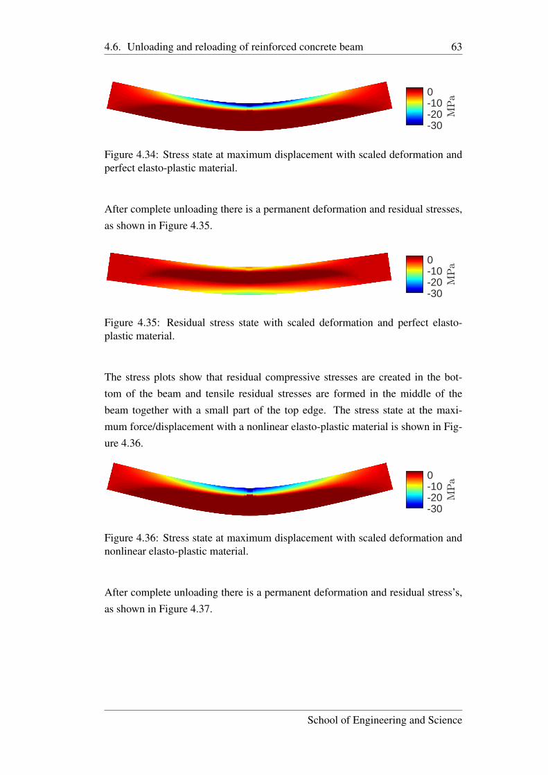
4.6. Unloading and reloading of reinforced concrete beam 63
-30-20-100
MPa
Figure 4.34: Stress state at maximum displacement with scaled deformation andperfect elasto-plastic material.
After complete unloading there is a permanent deformation and residual stresses,as shown in Figure 4.35.
-30-20-100
MPa
Figure 4.35: Residual stress state with scaled deformation and perfect elasto-plastic material.
The stress plots show that residual compressive stresses are created in the bot-tom of the beam and tensile residual stresses are formed in the middle of thebeam together with a small part of the top edge. The stress state at the maxi-mum force/displacement with a nonlinear elasto-plastic material is shown in Fig-ure 4.36.
-30-20-100
MPa
Figure 4.36: Stress state at maximum displacement with scaled deformation andnonlinear elasto-plastic material.
After complete unloading there is a permanent deformation and residual stress’s,as shown in Figure 4.37.
School of Engineering and Science
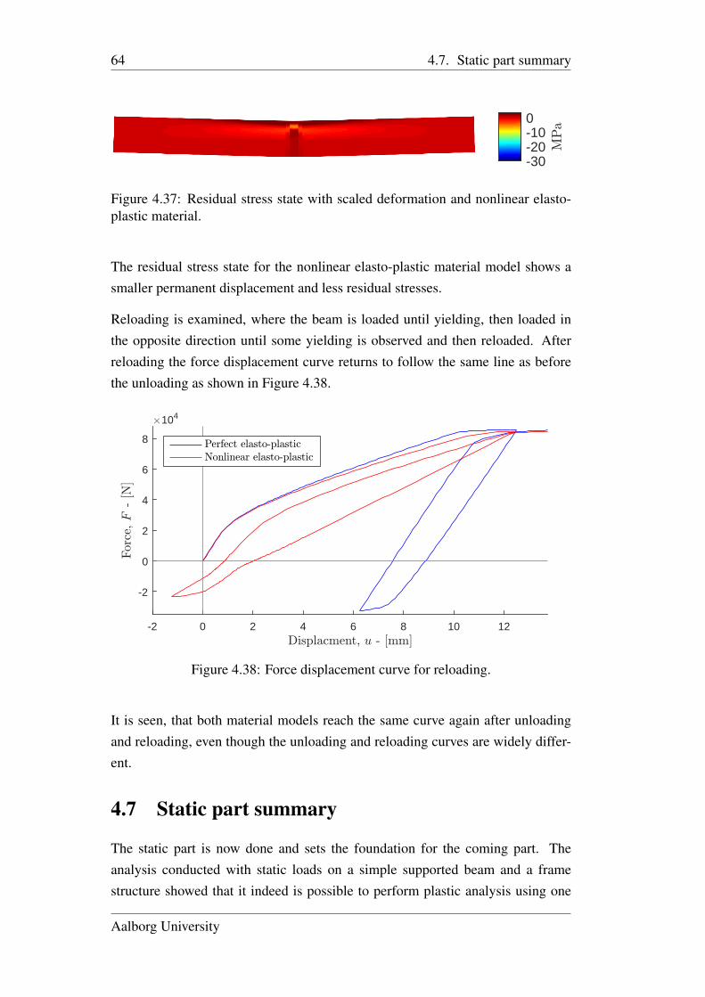
64 4.7. Static part summary
-30-20-100
MPa
Figure 4.37: Residual stress state with scaled deformation and nonlinear elasto-plastic material.
The residual stress state for the nonlinear elasto-plastic material model shows asmaller permanent displacement and less residual stresses.
Reloading is examined, where the beam is loaded until yielding, then loaded inthe opposite direction until some yielding is observed and then reloaded. Afterreloading the force displacement curve returns to follow the same line as beforethe unloading as shown in Figure 4.38.
Displacment, u - [mm]-2 0 2 4 6 8 10 12
For
ce,F
-[N
]
#104
-2
0
2
4
6
8 Perfect elasto-plastic Nonlinear elasto-plastic
Figure 4.38: Force displacement curve for reloading.
It is seen, that both material models reach the same curve again after unloadingand reloading, even though the unloading and reloading curves are widely differ-ent.
4.7 Static part summary
The static part is now done and sets the foundation for the coming part. Theanalysis conducted with static loads on a simple supported beam and a framestructure showed that it indeed is possible to perform plastic analysis using one
Aalborg University
4.7. Static part summary 65
dimensional finite element modelling. A MatLab script was developed, capableof performing gradual loading or increasing a forced displacement in incrementsso that the plastic behaviour during yielding could be described.
The analysis showed fair comparisons between an analytical solution to a simplesupported beam with a point load on the middle and the one-dimensional finiteelement solution performed in the MatLab script. Also, the Abaqus model gavesimilar results to the MatLab script.
The frame structure analysis showed that the MatLab script is able to handle morecomplex structures as well, also including plastic deformation.
Considering unloading and reloading, the MatLab script is definitely capable ofboth monotonic unloading and reloading of structures using both perfect elasto-plastic material behaviour and nonlinear elasto-plastic material behaviour. Here,the nonlinear material showed a larger recovered displacement, where the perfectelasto-plastic material has a steeper unloading/reloading curve. Though, the resultafter unloading and reloading was the same for both material models.
School of Engineering and Science

Part II
Dynamic finite-element analysis

69
Chapter 5
Introduction to dynamicsIn this chapter the dynamic part of the MatLab script is introduced and the nec-essary preparations are done to enable dynamics in the MatLab script. Dynamicfinite element models are often applied in earthquake engineering and when mod-elling traffic loads. The goal with this part of the MatLab script, is for it to beable to simulate the response of a reinforced concrete structure. A frame structuresubjected to ground accelerations recorded from a real earthquake and a railwaybridge subjected to a moving train is analysed.
Earlier, the material models where updated to handle unloading and reloading.This is necessary when considering plastic material, as the behaviour after plasticdeformation is reached, is crucial to the dynamic response of the system.
Solving dynamic problems require a nonlinear differential equation solver. Solverslike this could be a Runge-Kutta method, HHT-α or a Newmark-β method. Ap-plying schemes like these, the script becomes capable of numerical time integratethe dynamic response of a structure subjected to a load or displacement time se-ries. The dynamic theory is based the equation of motion as the governing equi-librium equation. The equation of motion is defined on the form:
[m]{u(t)}= { f ext(t)}−{ f int(t)}−{ f damp(t)}. (5.1)
Where [m] is the mass stiffness matrix and {u(t)} is the acceleration vector.{ f ext(t)} is the external forces acting on the system, { f int(t)} is the internal forcesand { f damp(t)} is the damping forces.
The internal forces and the damping forces can be found from
{ f int(t)}= [k]{u(t)}−{R}, (5.2)
{ f damp(t)}= [c]{u(t)}. (5.3)
Here, {R} is a nonlinear restoring force, [c] is the damping matrix, {u(t)} is the
School of Engineering and Science
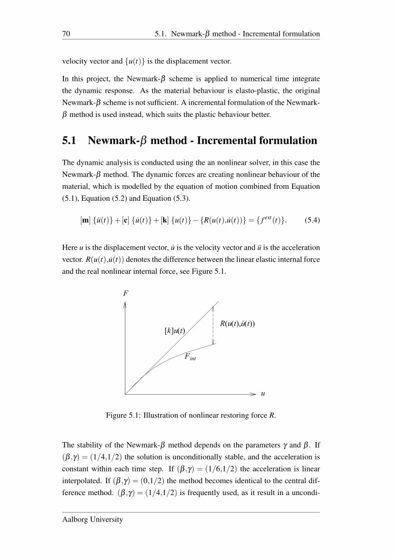
70 5.1. Newmark-β method - Incremental formulation
velocity vector and {u(t)} is the displacement vector.
In this project, the Newmark-β scheme is applied to numerical time integratethe dynamic response. As the material behaviour is elasto-plastic, the originalNewmark-β scheme is not sufficient. A incremental formulation of the Newmark-β method is used instead, which suits the plastic behaviour better.
5.1 Newmark-β method - Incremental formulation
The dynamic analysis is conducted using the an nonlinear solver, in this case theNewmark-β method. The dynamic forces are creating nonlinear behaviour of thematerial, which is modelled by the equation of motion combined from Equation(5.1), Equation (5.2) and Equation (5.3).
[m] {u(t)}+[c] {u(t)}+[k] {u(t)}−{R(u(t),u(t))}= { f ext(t)}. (5.4)
Here u is the displacement vector, u is the velocity vector and u is the accelerationvector. R(u(t),u(t)) denotes the difference between the linear elastic internal forceand the real nonlinear internal force, see Figure 5.1.
F
u
[k]u(t)
Fint
R(u(t),u(t)).
Figure 5.1: Illustration of nonlinear restoring force R.
The stability of the Newmark-β method depends on the parameters γ and β . If(β ,γ) = (1/4,1/2) the solution is unconditionally stable, and the acceleration isconstant within each time step. If (β ,γ) = (1/6,1/2) the acceleration is linearinterpolated. If (β ,γ) = (0,1/2) the method becomes identical to the central dif-ference method. (β ,γ) = (1/4,1/2) is frequently used, as it result in a uncondi-
Aalborg University
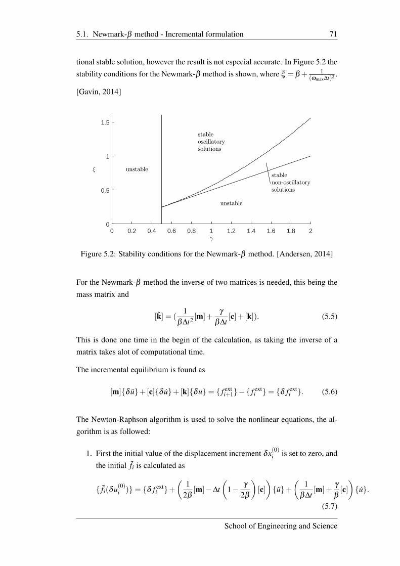
5.1. Newmark-β method - Incremental formulation 71
tional stable solution, however the result is not especial accurate. In Figure 5.2 thestability conditions for the Newmark-β method is shown, where ξ = β + 1
(ωmax∆t)2 .
[Gavin, 2014]
.0 0.2 0.4 0.6 0.8 1 1.2 1.4 1.6 1.8 2
9
0
0.5
1
1.5
unstable
stableoscillatorysolutions
stablenon-oscillatorysolutions
unstable
Figure 5.2: Stability conditions for the Newmark-β method. [Andersen, 2014]
For the Newmark-β method the inverse of two matrices is needed, this being themass matrix and
[k] = (1
β∆t2 [m]+γ
β∆t[c]+ [k]). (5.5)
This is done one time in the begin of the calculation, as taking the inverse of amatrix takes alot of computational time.
The incremental equilibrium is found as
[m]{δ u}+[c]{δ u}+[k]{δu}= { f exti+1}−{ f ext
i }= {δ f exti }. (5.6)
The Newton-Raphson algorithm is used to solve the nonlinear equations, the al-gorithm is as followed:
1. First the initial value of the displacement increment δx(0)i is set to zero, andthe initial fi is calculated as
{ fi(δu(0)i )}= {δ f exti }+
(1
2β[m]−∆t
(1− γ
2β
)[c]){u}+
(1
β∆t[m]+
γ
β[c]){u}.
(5.7)
School of Engineering and Science
72 5.1. Newmark-β method - Incremental formulation
2. The displacement increment is updated with
{δu(n+1)i }= [k]−1{ fi(δu(n)i )}, (5.8)
where
{ fi(δu(n)i )}= { fi(δu0i )}−{R
(n)i+1}+{Ri}, (5.9)
and the restoring force is updated with
{R(n)i+1}= [k]({ui}+{δu(n)i })−{ f int}. (5.10)
3. Step two is iterated upon until it converges, i.e. |{δu(n+1)i }−{δu(n)i }|< ε ,
where ε is the tolerance.
The displacements are updated with
{ui+1}= {ui}+{δui}, (5.11)
the velocities are updated with
{ui+1}= (1− γ
β){ui}−∆t(1− γ
2β){ui}+
γ
β∆t{δui}, (5.12)
and the accelerations are calculated as
{ui+1}=−[m]−1([c]{ui+1}+[k]{ui+1}−{Ri+1}−{ f exti+1}). (5.13)
This integration scheme, creates the basis for the dynamic calculations of a struc-ture with an elasto-plastic material model.
Aalborg University
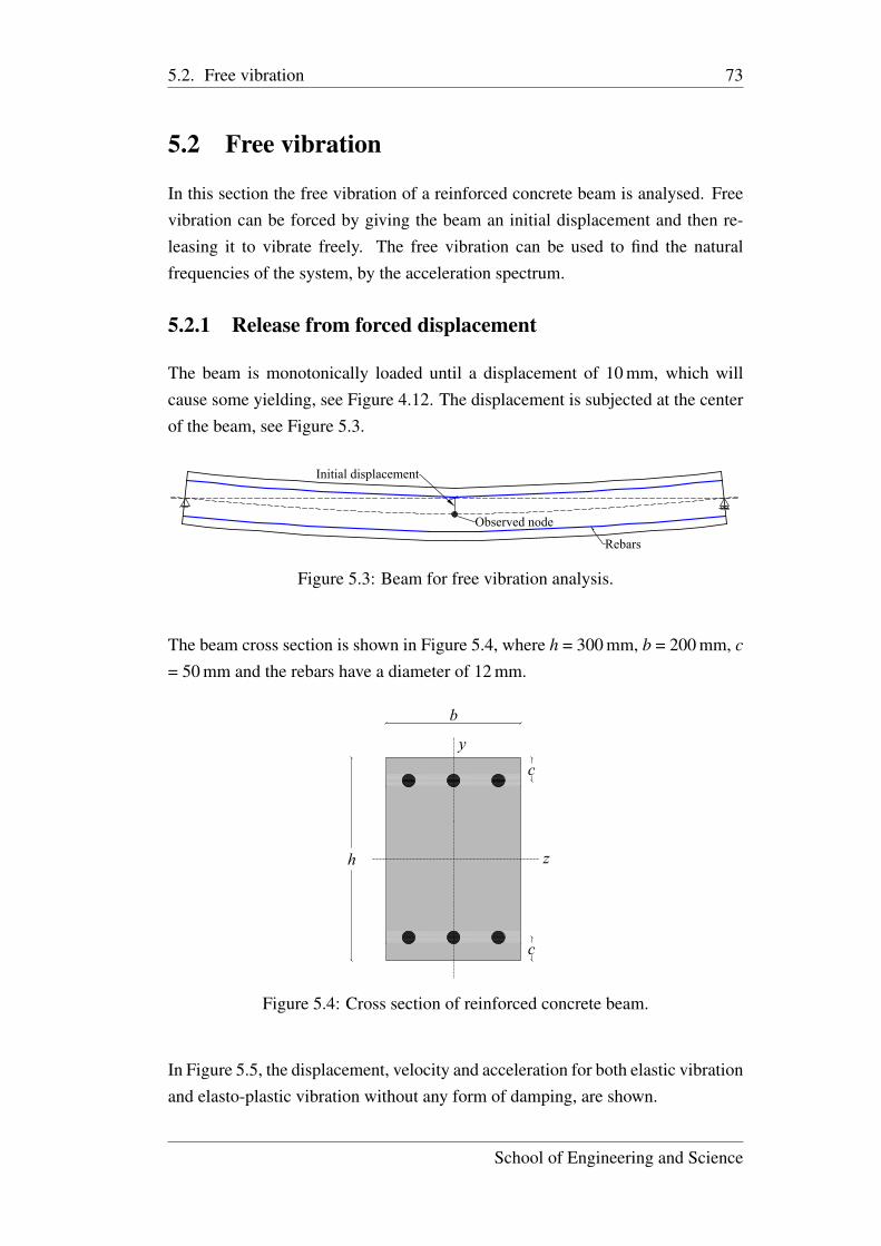
5.2. Free vibration 73
5.2 Free vibration
In this section the free vibration of a reinforced concrete beam is analysed. Freevibration can be forced by giving the beam an initial displacement and then re-leasing it to vibrate freely. The free vibration can be used to find the naturalfrequencies of the system, by the acceleration spectrum.
5.2.1 Release from forced displacement
The beam is monotonically loaded until a displacement of 10 mm, which willcause some yielding, see Figure 4.12. The displacement is subjected at the centerof the beam, see Figure 5.3.
Observed node
Initial displacement
Rebars
Figure 5.3: Beam for free vibration analysis.
The beam cross section is shown in Figure 5.4, where h = 300 mm, b = 200 mm, c
= 50 mm and the rebars have a diameter of 12 mm.
h
b
c
z
yc
Figure 5.4: Cross section of reinforced concrete beam.
In Figure 5.5, the displacement, velocity and acceleration for both elastic vibrationand elasto-plastic vibration without any form of damping, are shown.
School of Engineering and Science
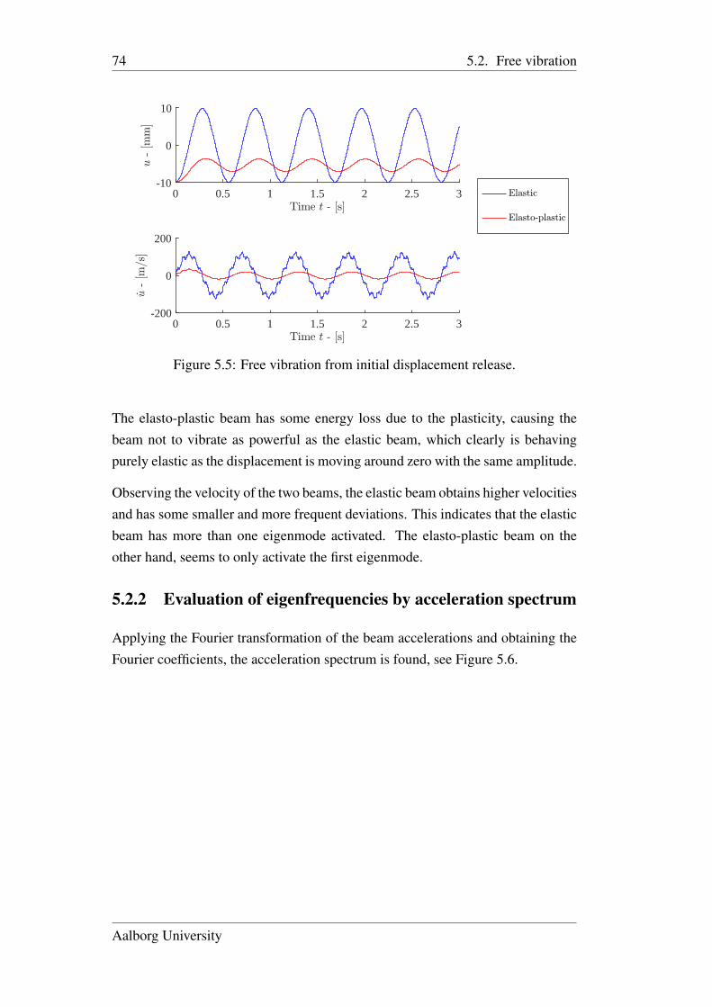
74 5.2. Free vibration
Time t - [s]0 0.5 1 1.5 2 2.5 3
u-[m
m]
-10
0
10
Elastic
Elasto-plastic
Time t - [s]0 0.5 1 1.5 2 2.5 3
_u-[m
/s]
-200
0
200
Figure 5.5: Free vibration from initial displacement release.
The elasto-plastic beam has some energy loss due to the plasticity, causing thebeam not to vibrate as powerful as the elastic beam, which clearly is behavingpurely elastic as the displacement is moving around zero with the same amplitude.
Observing the velocity of the two beams, the elastic beam obtains higher velocitiesand has some smaller and more frequent deviations. This indicates that the elasticbeam has more than one eigenmode activated. The elasto-plastic beam on theother hand, seems to only activate the first eigenmode.
5.2.2 Evaluation of eigenfrequencies by acceleration spectrum
Applying the Fourier transformation of the beam accelerations and obtaining theFourier coefficients, the acceleration spectrum is found, see Figure 5.6.
Aalborg University
5.2. Free vibration 75
Frequency [Hz]0 2 4 6 8 10 12S
pec
tral
den
sity #105
0
2
4Elasto-plastic
Frequency [Hz]0 2 4 6 8 10 12S
pec
tral
den
sity #106
0
1
2Elastic
Figure 5.6: Acceleration spectrum for elastic and elasto-plastic beam.
In the spectrum, a peak indicates a frequency where an eigenmode is activated andthe thereby the natural frequency for the given eigenmode is found.
The natural frequencies of the elastic and elasto-plastic beam are given in table5.1.
Table 5.1: Beam natural frequencies form acceleration spectrum.
Mode Elastic [Hz] Elasto-plastic [Hz]1 1.67 1.67
Natural frequency by stiffness and mass matrix
The model properties for evaluating the eigenfrequencies of the beam are given intable 5.2.
Table 5.2: Beam mass and volume properties.
Volume MassConcrete - ρ = 2400 kg/m3 1.79×10⁻² m3 430 kgRebars - ρ = 7800 kg/m3 1.0×10⁻³ m3 8 kgTotal 1.8×10⁻² m3 438 kg
The eigenfrequencies can be found from the stiffness matrix and mass matrix.
School of Engineering and Science
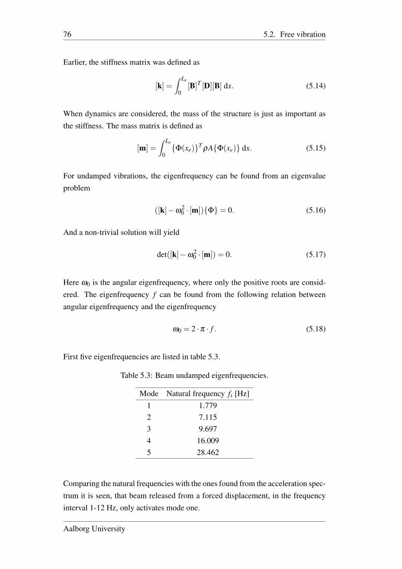
76 5.2. Free vibration
Earlier, the stiffness matrix was defined as
[k] =∫ Le
0[B]T [D][B] dx. (5.14)
When dynamics are considered, the mass of the structure is just as important asthe stiffness. The mass matrix is defined as
[m] =∫ Le
0{Φ(xe)}T
ρA{Φ(xe)} dx. (5.15)
For undamped vibrations, the eigenfrequency can be found from an eigenvalueproblem
([k]−ω20 · [m]){Φ}= 0. (5.16)
And a non-trivial solution will yield
det([k]−ω20 · [m]) = 0. (5.17)
Here ω0 is the angular eigenfrequency, where only the positive roots are consid-ered. The eigenfrequency f can be found from the following relation betweenangular eigenfrequency and the eigenfrequency
ω0 = 2 ·π · f . (5.18)
First five eigenfrequencies are listed in table 5.3.
Table 5.3: Beam undamped eigenfrequencies.
Mode Natural frequency fi [Hz]1 1.7792 7.1153 9.6974 16.0095 28.462
Comparing the natural frequencies with the ones found from the acceleration spec-trum it is seen, that beam released from a forced displacement, in the frequencyinterval 1-12 Hz, only activates mode one.
Aalborg University
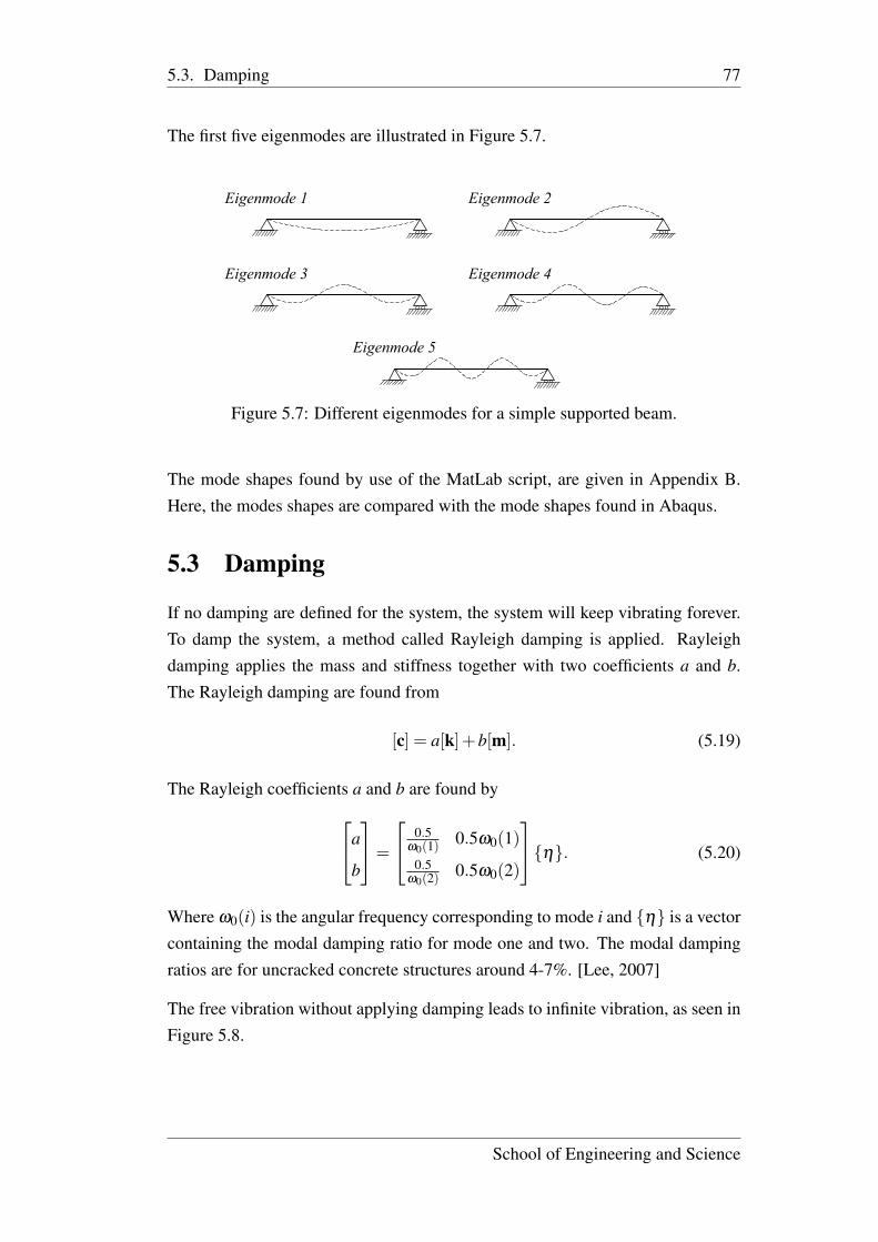
5.3. Damping 77
The first five eigenmodes are illustrated in Figure 5.7.
Eigenmode 1 Eigenmode 2
Eigenmode 3 Eigenmode 4
Eigenmode 5
Figure 5.7: Different eigenmodes for a simple supported beam.
The mode shapes found by use of the MatLab script, are given in Appendix B.Here, the modes shapes are compared with the mode shapes found in Abaqus.
5.3 Damping
If no damping are defined for the system, the system will keep vibrating forever.To damp the system, a method called Rayleigh damping is applied. Rayleighdamping applies the mass and stiffness together with two coefficients a and b.The Rayleigh damping are found from
[c] = a[k]+b[m]. (5.19)
The Rayleigh coefficients a and b are found bya
b
=
0.5ω0(1)
0.5ω0(1)0.5
ω0(2)0.5ω0(2)
{η}. (5.20)
Where ω0(i) is the angular frequency corresponding to mode i and {η} is a vectorcontaining the modal damping ratio for mode one and two. The modal dampingratios are for uncracked concrete structures around 4-7%. [Lee, 2007]
The free vibration without applying damping leads to infinite vibration, as seen inFigure 5.8.
School of Engineering and Science
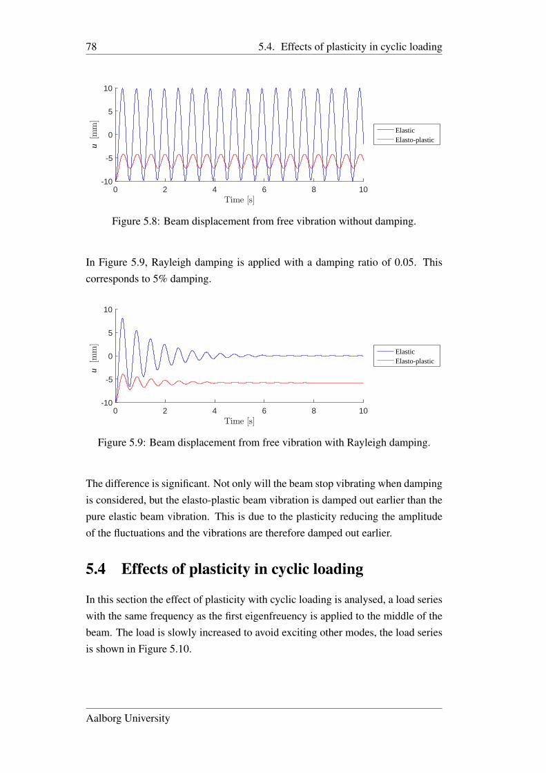
78 5.4. Effects of plasticity in cyclic loading
Time [s]0 2 4 6 8 10
[mm
]
-10
-5
0
5
10
ElasticElasto-plastic
u
Figure 5.8: Beam displacement from free vibration without damping.
In Figure 5.9, Rayleigh damping is applied with a damping ratio of 0.05. Thiscorresponds to 5% damping.
Time [s]0 2 4 6 8 10
[mm
]
-10
-5
0
5
10
ElasticElasto-plastic
u
Figure 5.9: Beam displacement from free vibration with Rayleigh damping.
The difference is significant. Not only will the beam stop vibrating when dampingis considered, but the elasto-plastic beam vibration is damped out earlier than thepure elastic beam vibration. This is due to the plasticity reducing the amplitudeof the fluctuations and the vibrations are therefore damped out earlier.
5.4 Effects of plasticity in cyclic loading
In this section the effect of plasticity with cyclic loading is analysed, a load serieswith the same frequency as the first eigenfreuency is applied to the middle of thebeam. The load is slowly increased to avoid exciting other modes, the load seriesis shown in Figure 5.10.
Aalborg University
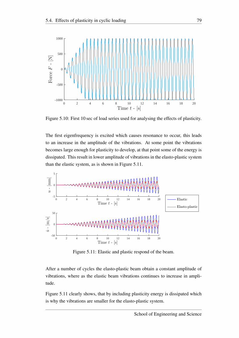
5.4. Effects of plasticity in cyclic loading 79
Time t - [s]0 2 4 6 8 10 12 14 16 18 20
For
ceF
-[N
]
-1000
-500
0
500
1000
Figure 5.10: First 10 sec of load series used for analysing the effects of plasticity.
The first eigenfrequency is excited which causes resonance to occur, this leadsto an increase in the amplitude of the vibrations. At some point the vibrationsbecomes large enough for plasticity to develop, at that point some of the energy isdissipated. This result in lower amplitude of vibrations in the elasto-plastic systemthan the elastic system, as is shown in Figure 5.11.
Time t - [s]0 2 4 6 8 10 12 14 16 18 20
u-[m
m]
-5
0
5
Elastic
Elasto-plastic
Time t - [s]0 2 4 6 8 10 12 14 16 18 20
_u-[m
/s]
-50
0
50
Figure 5.11: Elastic and plastic respond of the beam.
After a number of cycles the elasto-plastic beam obtain a constant amplitude ofvibrations, where as the elastic beam vibrations continues to increase in ampli-tude.
Figure 5.11 clearly shows, that by including plasticity energy is dissipated whichis why the vibrations are smaller for the elasto-plastic system.
School of Engineering and Science
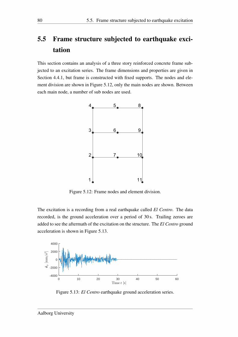
80 5.5. Frame structure subjected to earthquake excitation
5.5 Frame structure subjected to earthquake exci-tation
This section contains an analysis of a three story reinforced concrete frame sub-jected to an excitation series. The frame dimensions and properties are given inSection 4.4.1, but frame is constructed with fixed supports. The nodes and ele-ment division are shown in Figure 5.12, only the main nodes are shown. Betweeneach main node, a number of sub nodes are used.
1
2
3
4 8
9
10
5
6
7
11
Figure 5.12: Frame nodes and element division.
The excitation is a recording from a real earthquake called El Centro. The datarecorded, is the ground acceleration over a period of 30 s. Trailing zeroes areadded to see the aftermath of the excitation on the structure. The El Centro groundacceleration is shown in Figure 5.13.
Time t [s]0 10 20 30 40 50 60
Bag[m
m/s
2]
-4000
-2000
0
2000
4000
Figure 5.13: El Centro earthquake ground acceleration series.
Aalborg University
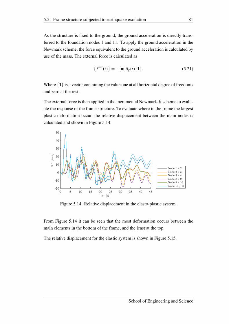
5.5. Frame structure subjected to earthquake excitation 81
As the structure is fixed to the ground, the ground acceleration is directly trans-ferred to the foundation nodes 1 and 11. To apply the ground acceleration in theNewmark scheme, the force equivalent to the ground acceleration is calculated byuse of the mass. The external force is calculated as
{ f ext(t)}=−[m]ag(t){1}. (5.21)
Where {1} is a vector containing the value one at all horizontal degree of freedomsand zero at the rest.
The external force is then applied in the incremental Newmark-β scheme to evalu-ate the response of the frame structure. To evaluate where in the frame the largestplastic deformation occur, the relative displacement between the main nodes iscalculated and shown in Figure 5.14.
t - [s]0 5 10 15 20 25 30 35 40 45
u-[m
m]
-20
-10
0
10
20
30
40
50
Node 1 / 2
Node 2 / 3
Node 3 / 4
Node 8 / 9
Node 9 / 10
Node 10 / 11
Figure 5.14: Relative displacement in the elasto-plastic system.
From Figure 5.14 it can be seen that the most deformation occurs between themain elements in the bottom of the frame, and the least at the top.
The relative displacement for the elastic system is shown in Figure 5.15.
School of Engineering and Science
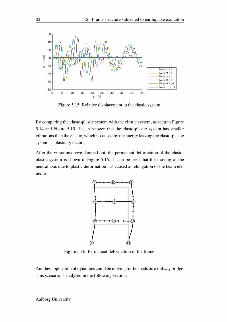
82 5.5. Frame structure subjected to earthquake excitation
t - [s]0 5 10 15 20 25 30 35 40 45
u-[m
m]
-80
-60
-40
-20
0
20
40
60
Node 1 / 2
Node 2 / 3
Node 3 / 4
Node 8 / 9
Node 9 / 10
Node 10 / 11
Figure 5.15: Relative displacement in the elastic system.
By comparing the elasto-plastic system with the elastic system, as seen in Figure5.14 and Figure 5.15. It can be seen that the elasto-plastic system has smallervibrations than the elastic, which is caused by the energy leaving the elasto-plasticsystem as plasticity occurs.
After the vibrations have damped out, the permanent deformation of the elasto-plastic system is shown in Figure 5.16. It can be seen that the moving of theneutral axis due to plastic deformation has caused an elongation of the beam ele-ments.
1
2
3
4 5
6
7
8
9
10
11
Figure 5.16: Permanent deformation of the frame.
Another application of dynamics could be moving traffic loads on a railway bridge.This scenario is analysed in the following section.
Aalborg University
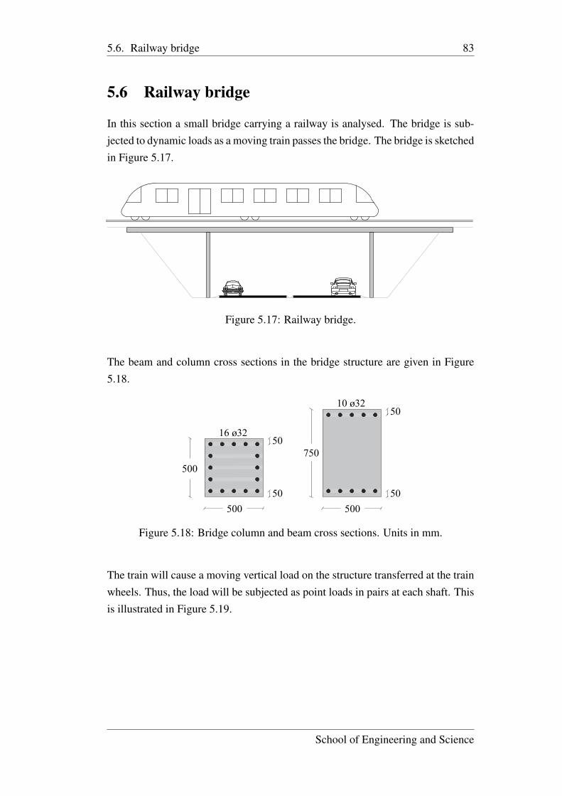
5.6. Railway bridge 83
5.6 Railway bridge
In this section a small bridge carrying a railway is analysed. The bridge is sub-jected to dynamic loads as a moving train passes the bridge. The bridge is sketchedin Figure 5.17.
Figure 5.17: Railway bridge.
The beam and column cross sections in the bridge structure are given in Figure5.18.
500750
500 500
16 ø32
10 ø3250
5050
50
Figure 5.18: Bridge column and beam cross sections. Units in mm.
The train will cause a moving vertical load on the structure transferred at the trainwheels. Thus, the load will be subjected as point loads in pairs at each shaft. Thisis illustrated in Figure 5.19.
School of Engineering and Science
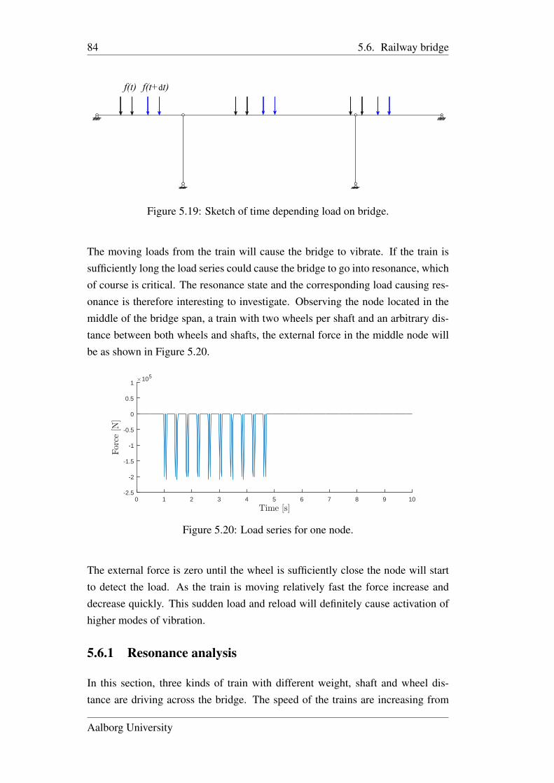
84 5.6. Railway bridge
f(t) f(t+dt)
Figure 5.19: Sketch of time depending load on bridge.
The moving loads from the train will cause the bridge to vibrate. If the train issufficiently long the load series could cause the bridge to go into resonance, whichof course is critical. The resonance state and the corresponding load causing res-onance is therefore interesting to investigate. Observing the node located in themiddle of the bridge span, a train with two wheels per shaft and an arbitrary dis-tance between both wheels and shafts, the external force in the middle node willbe as shown in Figure 5.20.
Time [s]0 1 2 3 4 5 6 7 8 9 10
For
ce[N
]
#105
-2.5
-2
-1.5
-1
-0.5
0
0.5
1
Figure 5.20: Load series for one node.
The external force is zero until the wheel is sufficiently close the node will startto detect the load. As the train is moving relatively fast the force increase anddecrease quickly. This sudden load and reload will definitely cause activation ofhigher modes of vibration.
5.6.1 Resonance analysis
In this section, three kinds of train with different weight, shaft and wheel dis-tance are driving across the bridge. The speed of the trains are increasing from
Aalborg University
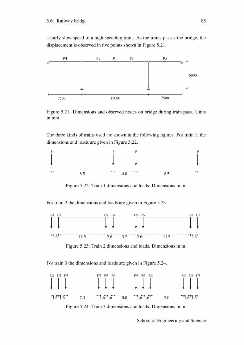
5.6. Railway bridge 85
a fairly slow speed to a high speeding train. As the trains passes the bridge, thedisplacement is observed in five points shown in Figure 5.21.
P4 P2 P1 P3 P5
6000
7500150007500
Figure 5.21: Dimensions and observed nodes on bridge during train pass. Unitsin mm.
The three kinds of trains used are shown in the following figures. For train 1, thedimensions and loads are given in Figure 5.22.
2.6 11.5 3.22.6 2.6 2.611.5
F/3
1.67.0 1.67.0 1.61.61.65.01.61.61.6
F/2F/2F/2 F/2F/2F/2F/2F/2
4.0
FFFF
8.5 8.5
F/3 F/3 F/3 F/3 F/3 F/3 F/3 F/3 F/3 F/3 F/3
Figure 5.22: Train 1 dimensions and loads. Dimensions in m.
For train 2 the dimensions and loads are given in Figure 5.23.
2.6 11.5 3.22.6 2.6 2.611.5
F/3
1.67.0 1.67.0 1.61.61.65.01.61.61.6
F/2F/2F/2 F/2F/2F/2F/2F/2
4.0
FFFF
8.5 8.5
F/3 F/3 F/3 F/3 F/3 F/3 F/3 F/3 F/3 F/3 F/3
Figure 5.23: Train 2 dimensions and loads. Dimensions in m.
For train 3 the dimensions and loads are given in Figure 5.24.
2.6 11.5 3.22.6 2.6 2.611.5
F/3
1.67.0 1.67.0 1.61.61.65.01.61.61.6
F/2F/2F/2 F/2F/2F/2F/2F/2
4.0
FFFF
8.5 8.5
F/3 F/3 F/3 F/3 F/3 F/3 F/3 F/3 F/3 F/3 F/3
Figure 5.24: Train 3 dimensions and loads. Dimensions in m.
School of Engineering and Science
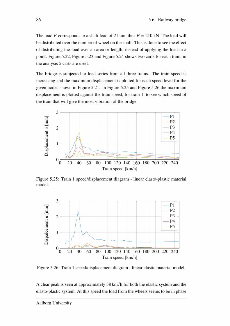
86 5.6. Railway bridge
The load F corresponds to a shaft load of 21 ton, thus F = 210 kN. The load willbe distributed over the number of wheel on the shaft. This is done to see the effectof distributing the load over an area or length, instead of applying the load in apoint. Figure 5.22, Figure 5.23 and Figure 5.24 shows two carts for each train, inthe analysis 5 carts are used.
The bridge is subjected to load series from all three trains. The train speed isincreasing and the maximum displacement is plotted for each speed level for thegiven nodes shown in Figure 5.21. In Figure 5.25 and Figure 5.26 the maximumdisplacement is plotted against the train speed, for train 1, to see which speed ofthe train that will give the most vibration of the bridge.
0 20 40 60 80 100 120 140 160 180 200 220 2400
1
2
3
Train speed [km/h]
Dis
plac
emen
tu[m
m] P1
P2P3P4P5
Figure 5.25: Train 1 speed/displacement diagram - linear elasto-plastic materialmodel.
0 20 40 60 80 100 120 140 160 180 200 220 2400
1
2
3
Train speed [km/h]
Dis
palc
emen
tu[m
m] P1
P2P3P4P5
Figure 5.26: Train 1 speed/displacement diagram - linear elastic material model.
A clear peak is seen at approximately 38 km/h for both the elastic system and theelasto-plastic system. At this speed the load from the wheels seems to be in phase
Aalborg University
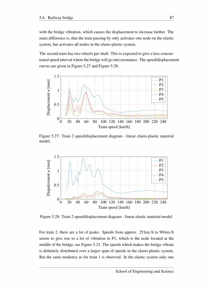
5.6. Railway bridge 87
with the bridge vibration, which causes the displacement to increase further. Themain difference is, that the train passing by only activates one node on the elasticsystem, but activates all nodes in the elasto-plastic system.
The second train has two wheels per shaft. This is expected to give a less concen-trated speed interval where the bridge will go into resonance. The speed/displacementcurves are given in Figure 5.27 and Figure 5.28.
0 20 40 60 80 100 120 140 160 180 200 220 2400
0.5
1
1.5
Train speed [km/h]
Dis
plac
emen
tu[m
m] P1
P2P3P4P5
Figure 5.27: Train 2 speed/displacement diagram - linear elasto-plastic materialmodel.
0 20 40 60 80 100 120 140 160 180 200 220 2400
0.5
1
1.5
Train speed [km/h]
Dis
palc
emen
tu[m
m] P1
P2P3P4P5
Figure 5.28: Train 2 speed/displacement diagram - linear elastic material model.
For train 2, there are a lot of peaks. Speeds from approx. 25 km/h to 90 km/hseems to give rise to a lot of vibration in P1, which is the node located at themiddle of the bridge, see Figure 5.21. The speeds which makes the bridge vibrateis definitely distributed over a larger span of speeds in the elasto-plastic system.But the same tendency as for train 1 is observed. In the elastic system only one
School of Engineering and Science
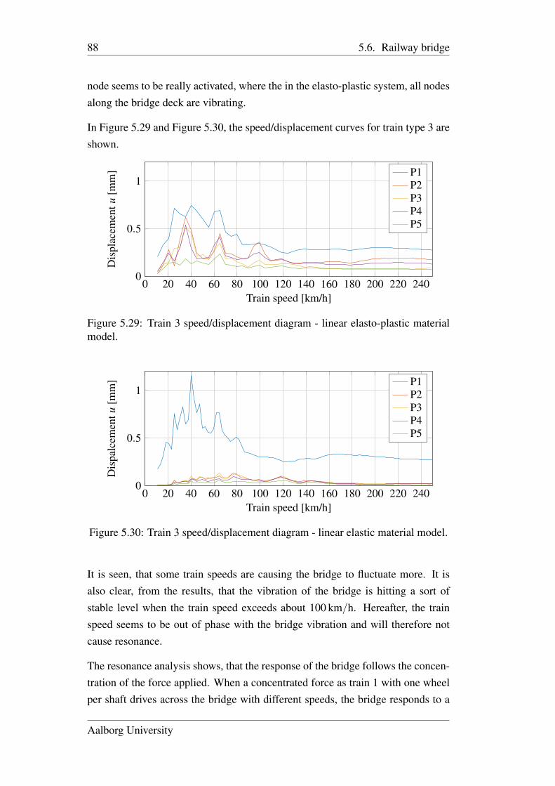
88 5.6. Railway bridge
node seems to be really activated, where the in the elasto-plastic system, all nodesalong the bridge deck are vibrating.
In Figure 5.29 and Figure 5.30, the speed/displacement curves for train type 3 areshown.
0 20 40 60 80 100 120 140 160 180 200 220 2400
0.5
1
Train speed [km/h]
Dis
plac
emen
tu[m
m] P1
P2P3P4P5
Figure 5.29: Train 3 speed/displacement diagram - linear elasto-plastic materialmodel.
0 20 40 60 80 100 120 140 160 180 200 220 2400
0.5
1
Train speed [km/h]
Dis
palc
emen
tu[m
m] P1
P2P3P4P5
Figure 5.30: Train 3 speed/displacement diagram - linear elastic material model.
It is seen, that some train speeds are causing the bridge to fluctuate more. It isalso clear, from the results, that the vibration of the bridge is hitting a sort ofstable level when the train speed exceeds about 100 km/h. Hereafter, the trainspeed seems to be out of phase with the bridge vibration and will therefore notcause resonance.
The resonance analysis shows, that the response of the bridge follows the concen-tration of the force applied. When a concentrated force as train 1 with one wheelper shaft drives across the bridge with different speeds, the bridge responds to a
Aalborg University
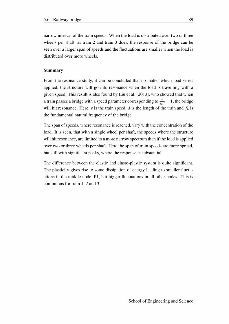
5.6. Railway bridge 89
narrow interval of the train speeds. When the load is distributed over two or threewheels per shaft, as train 2 and train 3 does, the response of the bridge can beseen over a larger span of speeds and the fluctuations are smaller when the load isdistributed over more wheels.
Summary
From the resonance study, it can be concluded that no matter which load seriesapplied, the structure will go into resonance when the load is travelling with agiven speed. This result is also found by Liu et al. [2013], who showed that whena train passes a bridge with a speed parameter corresponding to v
fbd = 1, the bridgewill hit resonance. Here, v is the train speed, d is the length of the train and fb isthe fundamental natural frequency of the bridge.
The span of speeds, where resonance is reached, vary with the concentration of theload. It is seen, that with a single wheel per shaft, the speeds where the structurewill hit resonance, are limited to a more narrow spectrum than if the load is appliedover two or three wheels per shaft. Here the span of train speeds are more spread,but still with significant peaks, where the response is substantial.
The difference between the elastic and elasto-plastic system is quite significant.The plasticity gives rise to some dissipation of energy leading to smaller fluctu-ations in the middle node, P1, but bigger fluctuations in all other nodes. This iscontinuous for train 1, 2 and 3.
School of Engineering and Science

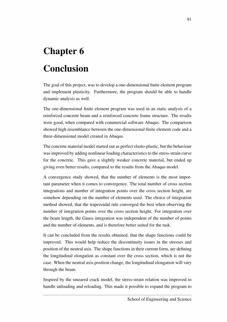
91
Chapter 6
ConclusionThe goal of this project, was to develop a one-dimensional finite element programand implement plasticity. Furthermore, the program should be able to handledynamic analysis as well.
The one-dimensional finite element program was used in an static analysis of areinforced concrete beam and a reinforced concrete frame structure. The resultswere good, when compared with commercial software Abaqus. The comparisonshowed high resemblance between the one-dimensional finite element code and athree-dimensional model created in Abaqus.
The concrete material model started out as perfect elasto-plastic, but the behaviourwas improved by adding nonlinear loading characteristics to the stress-strain curvefor the concrete. This gave a slightly weaker concrete material, but ended upgiving even better results, compared to the results from the Abaqus model.
A convergence study showed, that the number of elements is the most impor-tant parameter when it comes to convergence. The total number of cross sectionintegrations and number of integration points over the cross section height, aresomehow depending on the number of elements used. The choice of integrationmethod showed, that the trapezoidal rule converged the best when observing thenumber of integration points over the cross section height. For integration overthe beam length, the Gauss integration was independent of the number of pointsand the number of elements, and is therefore better suited for the task.
It can be concluded from the results obtained, that the shape functions could beimproved. This would help reduce the discontinuity issues in the stresses andposition of the neutral axis. The shape functions in their current form, are definingthe longitudinal elongation as constant over the cross section, which is not thecase. When the neutral axis position change, the longitudinal elongation will varythrough the beam.
Inspired by the smeared crack model, the stress-strain relation was improved tohandle unloading and reloading. This made it possible to expand the program to
School of Engineering and Science
92 Chapter 6. Conclusion
include elasto-plastic dynamic analysis as well.
The free vibration study showed, that the plasticity will lead to some dissipation inenergy. This energy dissipation will cause the beam to fluctuate less than a beamwhich is purely elastic.
The earthquake study of a frame structure showed the same behaviour. The energydissipation will cause the frame structure to have smaller vibrations and damp outearlier.
The train bridge study showed larger vibration in the middle of the bridge forthe elastic case, however the elasto-plastic system showed more vibration furtheraway form the middle. Also, the bridge study showed, that more concentratedloads, e.g. Train 1, will cause bigger displacements and a more clear peak whenthe train speed cause the bridge to go into resonance. Including plasticity, willlead to a build up in displacement in the bridge deck. Including plasticity, willgive a more realistic response of the system, as the energy dissipation will lead tomore authentic vibrations.
Aalborg University
93
Chapter 7
Reference Lists
BibliographyAndersen, 2014. Lars Andersen. Structural mechanics and dynamics. Course
material and MATLAB codes, 2014.
Gavin, 2014. Henri P. Gavin. Numerical Integration in Structural Dynamics.URL : http://people.duke.edu/hpgavin/cee541/NumericalIntegration.pdf, 2014.24-05-2016.
Jensen, 2012. Bjarne Chr. Jensen. Betonkonstruktioner efter DS/EN 1992-1-1.ISBN-13: 9788757127669, Handbook. Nyt teknisk forlag, 2012.
Krabbenhøft, 2002. Kristian Krabbenhøft. Basic Computational Plasticity.Department of Civil Engineering - Technical University of Denmark, 2002.
Lee, 2007. Yi-Kuen Lee. DAMPING CROSS-REFERENCE. URL :http://teaching.ust.hk/mech300/mech300_7_1_damping_ref.pdf, 2007.16-05-2016.
Liu, Zhou, Shi, Wang, Shi, og Roeck, 2013. K. Liu, H. Zhou, G. Shi, Y.Q.Wang, Y.J. Shi, og G. De Roeck. Fatigue assessment of a composite railway
bridge for high speed trains. Part II: Conditions for which a dynamic analysis
is needed. Journal of Constructional Steel Research, 82, 246 – 254, 2013.ISSN 0143-974X. doi: http://dx.doi.org/10.1016/j.jcsr.2012.11.014. URLhttp://www.sciencedirect.com/science/article/pii/
S0143974X1200274X.
Mohamad, Farid, og Al-Janabi, 1990. Anis Mohamad, B.J. Farid, og A.J.M.Al-Janabi. Stress-Strain Relationship for Concrete in Compression Made of
Local Materials. Department of Civil Engineering - University of Basrah,Iraq, 1990.
School of Engineering and Science

94 Bibliography
Poulsen og Olesen, 2015. Peter Noe Poulsen og John Forbes Olesen. Bærende
konstruktioner 1 - Statisk bestemte stænger og bjælker. ISBN:978-87-502-1107-5, Handbook. Polyteknisk Forlag, 2015.
SIMULIA, 2014. SIMULIA. Abaqus Theory Guide. URL :http://130.149.89.49:2080/v6.14/books/stm/default.htm?startat=ch04s05ath119.html,2014. 31-05-2016.
Williams og Todd, 1999. Martin S. Williams og J. D. Todd. Structures: Theory
and Analysis. ISBN: 9780333677605. Palgrave Macmillan, 1999.
Aalborg University

Part III
Appendix


97
Appendix A
Abaqus modellingIn this chapter a model is created in commercial software Abaqus. Abaqus is awidely used program for analysing complex structures in practise and will giveresults to compare the model created in MatLab.
Abaqus offers many choices regarding element types, geometry, boundary con-ditions and load apply etc. and can be modelled to match the model in MatLab.Though, Abaqus is not capable of analysing one dimensional reinforced concretemodels, the comparison with the MatLab program will not be entirely fair. Thus,the boundary conditions, element type and apply of load must be set up equallyfor both models.
A.1 Model
For the Abaqus model, a 3D model is chosen. This is done to compare the MatLabscript against a model with a much higher complexity.
A.1.1 Boundary conditions
The boundary conditions is simple supports, implying pinned support at one edgeand roller support at the second edge. The model boundary conditions are illus-trated in Figure A.1.
y0h
L
u
Rebars
Figure A.1: Abaqus statical system.
At the right edge a support with roller is applied along the z axis to prevent dis-placement in the transversal directions. The roller is important to make the systemstatically determined.
School of Engineering and Science
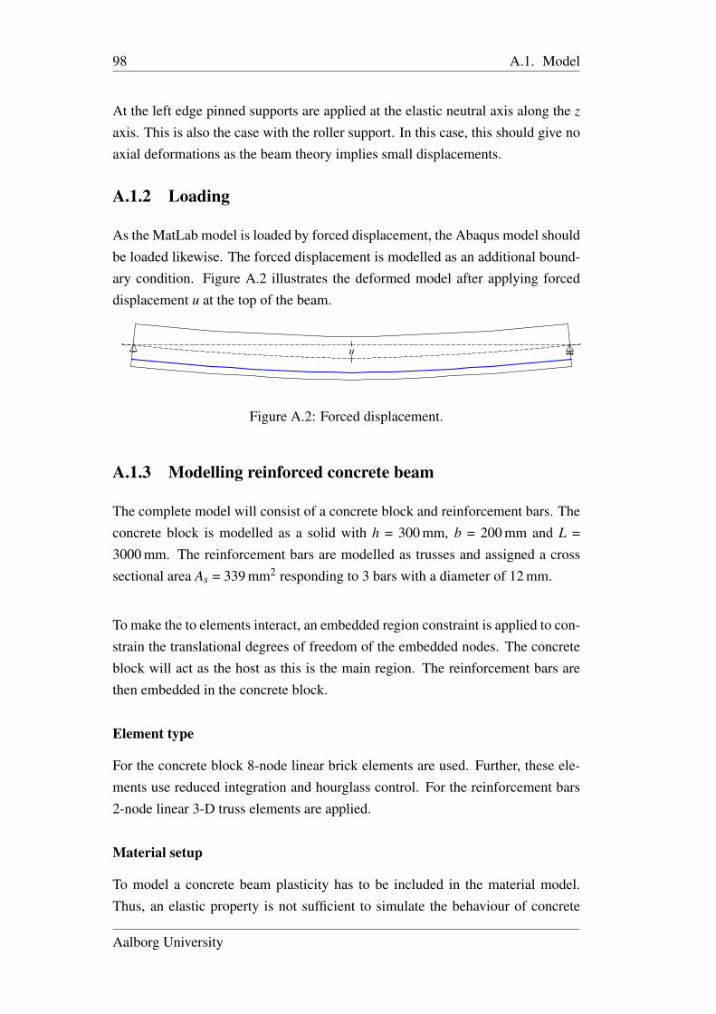
98 A.1. Model
At the left edge pinned supports are applied at the elastic neutral axis along the z
axis. This is also the case with the roller support. In this case, this should give noaxial deformations as the beam theory implies small displacements.
A.1.2 Loading
As the MatLab model is loaded by forced displacement, the Abaqus model shouldbe loaded likewise. The forced displacement is modelled as an additional bound-ary condition. Figure A.2 illustrates the deformed model after applying forceddisplacement u at the top of the beam.
y0h
L
u
Rebars
Figure A.2: Forced displacement.
A.1.3 Modelling reinforced concrete beam
The complete model will consist of a concrete block and reinforcement bars. Theconcrete block is modelled as a solid with h = 300 mm, b = 200 mm and L =3000 mm. The reinforcement bars are modelled as trusses and assigned a crosssectional area As = 339 mm2 responding to 3 bars with a diameter of 12 mm.
To make the to elements interact, an embedded region constraint is applied to con-strain the translational degrees of freedom of the embedded nodes. The concreteblock will act as the host as this is the main region. The reinforcement bars arethen embedded in the concrete block.
Element type
For the concrete block 8-node linear brick elements are used. Further, these ele-ments use reduced integration and hourglass control. For the reinforcement bars2-node linear 3-D truss elements are applied.
Material setup
To model a concrete beam plasticity has to be included in the material model.Thus, an elastic property is not sufficient to simulate the behaviour of concrete
Aalborg University
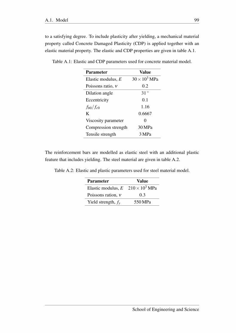
A.1. Model 99
to a satisfying degree. To include plasticity after yielding, a mechanical materialproperty called Concrete Damaged Plasticity (CDP) is applied together with anelastic material property. The elastic and CDP properties are given in table A.1.
Table A.1: Elastic and CDP parameters used for concrete material model.
Parameter ValueElastic modulus, E 30×103 MPaPoissons ratio, ν 0.2Dilation angle 31 ◦
Eccentricity 0.1fb0/ fc0 1.16K 0.6667Viscosity parameter 0Compression strength 30 MPaTensile strength 3 MPa
The reinforcement bars are modelled as elastic steel with an additional plasticfeature that includes yielding. The steel material are given in table A.2.
Table A.2: Elastic and plastic parameters used for steel material model.
Parameter ValueElastic modulus, E 210×103 MPaPoissons ration, ν 0.3Yield strength, fy 550 MPa
School of Engineering and Science

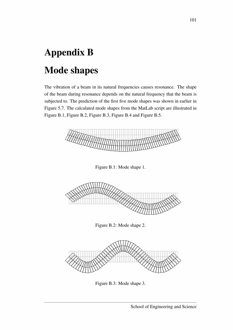
101
Appendix B
Mode shapesThe vibration of a beam in its natural frequencies causes resonance. The shapeof the beam during resonance depends on the natural frequency that the beam issubjected to. The prediction of the first five mode shapes was shown in earlier inFigure 5.7. The calculated mode shapes from the MatLab script are illustrated inFigure B.1, Figure B.2, Figure B.3, Figure B.4 and Figure B.5.
Figure B.1: Mode shape 1.
Figure B.2: Mode shape 2.
Figure B.3: Mode shape 3.
School of Engineering and Science
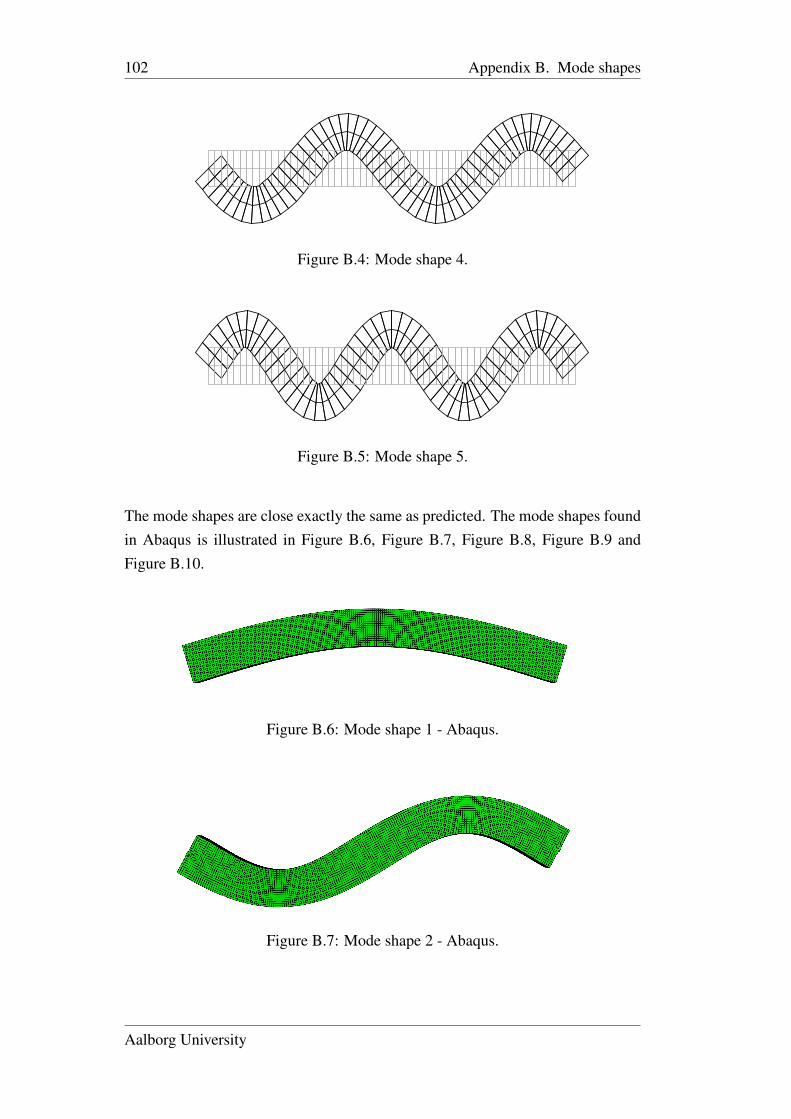
102 Appendix B. Mode shapes
Figure B.4: Mode shape 4.
Figure B.5: Mode shape 5.
The mode shapes are close exactly the same as predicted. The mode shapes foundin Abaqus is illustrated in Figure B.6, Figure B.7, Figure B.8, Figure B.9 andFigure B.10.Printed using Abaqus/CAE on: Fri May 06 13:18:17 Romance Daylight Time 2016
Figure B.6: Mode shape 1 - Abaqus.Printed using Abaqus/CAE on: Fri May 06 13:21:01 Romance Daylight Time 2016
Figure B.7: Mode shape 2 - Abaqus.
Aalborg University
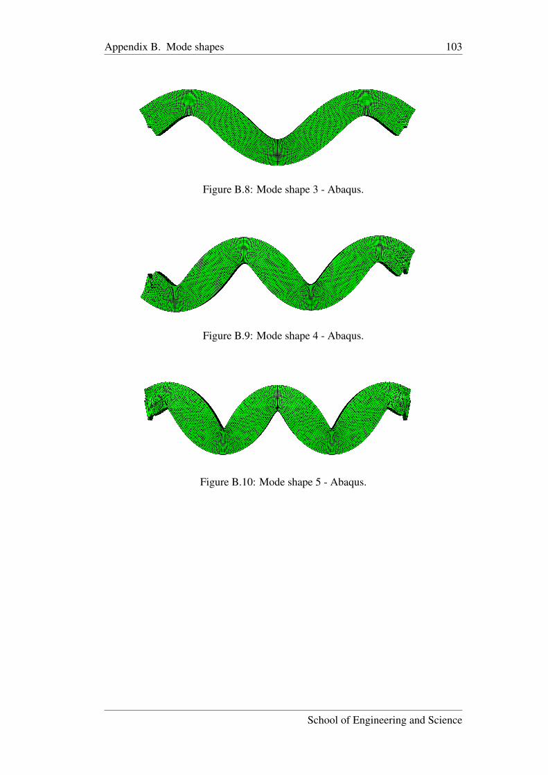
Appendix B. Mode shapes 103Printed using Abaqus/CAE on: Fri May 06 13:21:18 Romance Daylight Time 2016
Figure B.8: Mode shape 3 - Abaqus.Printed using Abaqus/CAE on: Fri May 06 13:21:30 Romance Daylight Time 2016
Figure B.9: Mode shape 4 - Abaqus.Printed using Abaqus/CAE on: Fri May 06 13:21:43 Romance Daylight Time 2016
Figure B.10: Mode shape 5 - Abaqus.
School of Engineering and Science

105
Appendix C
Digital appendix
C.1 MatLab scripts
• Functions
• Graph
• Beam_1D_Dynamic_beam.m
• Beam_1D_Dynamic_bridge.m
• Beam_1D_Dynamic_frame.m
• Beam_1D_Static_Disp.m
• Beam_1D_Static_force.m
• elcentro.dat
• input_beam.m
• input_beam_force.m
• input_bridge.m
• input_frame.m
C.2 Abaqus model
• RC_beam.cae
School of Engineering and Science