SSC-345(PART 1)

ELASTIC - PLASTIC

FRACTURE MECHANICSA CRITICAL REVIEW

This document has been approvedfor public release and sale; its

distribution is unlimited

SHIP STRUCTURE COMMITTEE

1990

SHIP STRUCTURE COMMllTFF

The SHIP STRUCTURE COMMlllEE is constitutedto prosecutea researchprogramto improvethe hullstructuresof shipsand othermarinestructuresby an extensionof knowledgepertainingto design,materials,and methodsof construction.

‘M’” ‘“‘r’“SCG’‘Chairmw)Chief, Office o Marine Safety, Securityand EnvironmentalProtection

U.S. Coast Guard

Mr. AlexanderMalakhoffDirector,StructuralIntegrity

Subgroup(SEA 55Y)Naval Sea SystemsCommand

Dr. Donald LiuSeniorVice PresidentAmerican Bureauof Shipping

Mr. H. T. HatlerAsmiate Administratorfor Ship-

buildingand Ship OperationsMaritimeAdministration

Mr. Thomas W. AllenEngineeringOfhcer(N7)MilitarySealiftCommand

CDR Michael K. Parmelee, USCG,Secretary,Ship StructureCommitteeU.S. Coast Guard

C C G OFFICER TECHN CAL RF ~$ENTA IVF$ONTRA TIN I P T

Mr. WilliamJ. SiekierkaSEA55Y3

Mr. Greg D. WoodsSEA55Y3

Naval Sea SystemsCommand Naval Sea SystemsCommand

SHIP STRUCTURE SURCOMMllTEE

The SHIP STRUCTURE SUBCOMMITTEE acts for the Ship StructureCommitteeon technicalmattersby providingtechnicalcoordinationfor determinatingthe goals and objectivesof the programand by evaluatingend interpretingthe resultsintermsof structuraldesign,construction,and operation.

AMFRICAN BURFAU O!= SHIPPING

Mr. Stephen G. Arntson(Chairman)Mr. John F. ConIonMr. William HaruelekMr. PhilipG. Rynn

MILITARY SEALlm COMMAND

Mr. AlbertJ, AttermeyerMr. MichaelW. ToumaMr. Jeffery E, Beach

Mr. RobertA SielskiMr. Charles L. NullMr. W. Thomas PackardMr. Allen H. Engle

U.S. COAST GUARD

CAPT T. E. ThompsonCAPT DonaldS. JensenCDR Mark E. Nell

MARITIME ADMINISTRATION

Mr. FrederickSeiboldMr. Norman0. HammerMr. Chao H. LinDr. Walter M. Maclean

SHIP STRUCTURE SUBCOMMllTEE LIAISON MEMBERS

U. S. COAST GUARD ACADEMY

LT BruceMustain

U. S, MFRCHANT MARINF ACADFMY

Dr. C, B, Kim

U. S. NAVAL ACADEMY

Dr. Ramswar Bhattacharyya

Dr. W. R. Porter

WELDING RESEARCH COUNCIL

Dr. Martin Prager

WTIOH ACADEMY OF SCIENCES -MARINEBOARD

Mr. Alexander B. Stavovy

NATIONAL ACADEMY OF SCIENCES -COMMllTE E ON MARINE STRUCTURES

Mr. Stanley G. Stiansen

s~

j-hYDRODYNAMICSCOMMllTEF

Dr. WilliamSandberg

wFRICAN IRON AND STFFI INSTITUTF

Mr. AlexanderD. Wilson

Member Agencies:

United States Coast GuardNaval Saa Systems Command

Matitime AdministrationAmerkan Bureau of Sh@ing

Militq Sealti Command

& Address tirres~ndence to:

Smetary, Ship Structure Committee

ShipU.S. baa? Guard (G-MTH)2100 Second Street S.W.

Structure Washington, D.C. 20593-0001PH: (202) 257-@m

Committee FAX (202) 267-0025

An InteragencyAdvisoryCommitteeDedicatedto the Improvementof MarfneStructures

SSC-345December 17, 1990 SR-1321

ELASTIC-PLASTIC FRACTURE MECHANICSA CRITICAL REVIEW

The use of fracture mechanics as a tool for structural design andanalysis has increased significantly in recent years. Fracturetheories provide relationships among fracture toughness, stress,and flaw size and are used, for example, to establish acceptancestandards for material defects in structures. This first part ofa two part report provides a critical review of the history andstate-of-the-art of elastic-plastic fracture mechanics. Part 2presents the results of an analytical and experimental study offracture in the ductile-brittle transition zone of hull steels.

*Rear Admiral, U.S. Coast Guard

Chairman, Ship Structure Comittee

Technicol Report Documentation Poge

1. Report No. 2. Government Accession No.

SSC-345 - Part 1I

4. T,tle and Subtitle

Elastic-Plastic Fracture Mechanics -A Critical Review

~.Authds)

T. L. Anderson

9. Performing Organization Name and Address

Texas A & M Research FoundationP. O. BOX 3578College Station, TX 77843

‘?kii~ii’??$?i~’N.., m, .,,j,=..

U.S. Coast Guard2100 Second Street, SWWashington, DC 20593

3. Recipient’s Catalog No..-

5. Report D.te

April 1990

6. Performing Organization Code

—S. Performing Orgotiization Report No.

SR-1321

10. Wark Unit No. (T RAIS)

11. Contract or Grant No.

DTCG23-88-C-2003713. Typeef Reportond Peried Covered

Final Report

14. Sponsoring Agc”cy Cndc

G-M

15. SuPPlementarYNote$

Sponsored by the Ship Structure Committee and its member agencies.

16. Abstruct

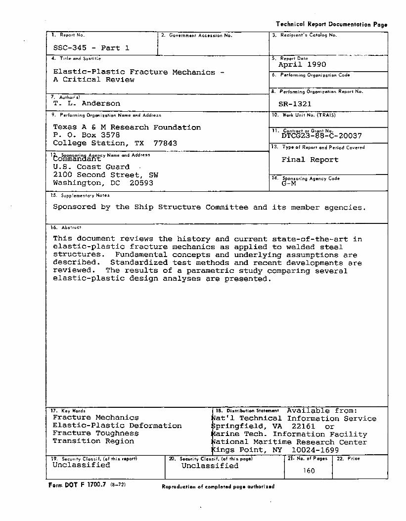
This document reviews the history and current state-of-the-art inelastic-plastic fracture mechanics as applied to welded steelstructures. Fundamental concepts and underlying assumptions aredescribed. Standardized test methods and recent developments arereviewed. The results of a parametric study comparing severalelastic-plastic design analyses are presented.

17. Key Words 18. Distribution Statement Available from:Fracture Mechanics Jat’1 Technical Information ServiceElastic-Plastic Deformation Springfield, VA 22161 orFracture Toughness I~arine Tech. Information FacilityTransition Region ,~ational Maritime Research Center

ings Point, NY 10024-169919. Security Classic. (ofthisr*pert) ~. Security Classic. (of this page) 21. No. of Pages 22. Price

Unclassified Unclassified160

Form DOT F 1700.7 (8-72) Reproduction ofcompleted pogeouthorized

1

METRIC COWEHSI(IN FACTORS

Srmbd

LENGTH

LEHIIT+Im

ml

x’”m

km

mnl~irmters 0.04cmnlirnctara 0.4InMers 3.3nwmrs 1.1k[lomdats 0.6

mchas “2.5ieat 20

v-d- 0.9mi ks 1.6

cm tinwlws

cenaNIW1*M

mmersk,hmntmrm

cmcmmkm

cma#

Jha

ha

eh9i

ml

mlml

IIi

4~3

m’

“c

MEAC#

G#~2

ru

2qu2c* C4ntkmmts 0.18squm* mlws 1.22quu0 kilmrw.tmb9ctu4s IIo,ooo A R

in2

F#

yd2mia

MASS (weight)

UJncm* 23pared, 0.46short Ims 0.9

Imlo lb)

VOIUME

gramsgmmm 0.036htl~ms 2.2

timwws 11~ kg) 1.*

9kgI

92

lb k!kqmmsh-mm

VOUIME

Imm,fmam 6

me Impoms 15fluid Wmc,, 30cups 0.24pmls 0.47quarFn 0.95Omllms 3.Bcubic fnef 0.03cubic yards 0.76

TEMPEflATURE (omct~

milhlihm 0.03Iimm 2.1#imvs 1SmI,WIS 0.26cubm nwlarn 35cubic nmmts 9.3

lap

Tbsp!1 Oz

cplqt

gal813vdJ

milliliters

mi!Iiliw*mil~ilimrs

IittmIilarstiqers

Iiierscub,c mewscubic meters

mlII

:3Ill’

“c Celsius 9/6 ohm

twralum Al 321“f Fahmnhei I s/9 Iaftmr

tomwram m subtracting

32) OF 32 9a6

-40 0 40 00 I2

k~-40 -20 0 20 40

“c 37

EXECUTIVE SUMMARY

This document reviews the history and current state of the art in elastic-plastic fracture mechani~, as applied to welded steel structur~. FM, thefundamental concepts and underlying assumptions of fracture mechanie ared=uibed. A review of fracture mdarb -t methods follows, includingstandardized test methmis as well as recent dev~opments that are not yetstandard practice+ N- the various prmedum for applying fra~medumi~ conceps to strum are outlined. The rssults of a parametricstudy whida compars several elastic-plastic design analp are presmted.This review has led to a numk of conclusions and recommendations.

The ductikbrittle transition region is the critical area of concern for weldedsteel structure.. If the material is on the lower shelf of toughness, it is usuallytoo brittle for structural application; if it is on the upper shelf, fracture willnot be a significant problem in most structural steels. One difikulty withapplying fracture mechani~ to welded structures in the transition region isthe lack of standardized fracture toughrws test procedure for weldments. hadditional problem is that the size dependence of fracture toughness in thetransition region has not been quantified. Scatter of toughness data in the

Iower transition region is reasonably well understood, but the uppertmnsition region introduces compltities that require further study.

The comparison of elastic-plastic fracture analyses revealed that predictedfailure str=s and critical aa& size are insensitive to the analysis equation.Under linear elastic conditions, dl anal- were identical. In the otherextreme of fully plastic conditions, the analy~ approached similar collapselimits. Since most elastic-plastic fracture anslysis equations predict similarr~ults, the sixnpl~t equation seems to k most appropriate.

Current elastic-plastic fracture analy- tend to be consemative when appliedto complex welded structures. In order to improve their accuracy, a numberof issues need to be addressed the driving force in wekhnents, residual stressmeasurements, three-dimensional effects, gross-seclion yielding and mack tipconstraint

1.

z

3.

TABLE OF CONTENTS

INTRQDUCTTON .""... **.*.*.**..".*".. *.."" "" . ...."...* ...........................*....*.****"0*.."" ***........1

FUNDAMENTAL CONCEFTS..

...***...".." " . . ..".* *.*. "...* . . . . . . . . . . ..""" .*"w.. ***... **** . . ..""** . . . . . . . 4

21

22

23

24

ENERGY APPROACH TO FM@TURE W~G ....--..- ..... . ..-..-..4

STRESS INTENS~ APPROACH TO PMCTURE MECHANICS ...........6

E’MSITC-P’MSTIC FmcTuRE MKHANIcs .... ........................................1023.123.223.323.423.523.623.723.8

M Plastic Zone Correction .......*..*..******..*.......................................10Strip Meld Plastic Zone Cmmction ..................**.**..*.*******..................13Plastic Zone Shape ****. .......*....***............................................................14Crack Tlp Opning Displacement .....................*...*.**.**..*.......*.**.*****●*16The J Contour Integral ●*..*..*...............**..****●***.*. ...................................17.Relationship Between J and ~OD 20....................................................The Effect of Yielding on Crack TIp %r~ Fields .......*.*****..............21Effect of Thickness on Crack Tip StrSs Fields .................... ............25

MtCROMECHAMSM5 OF FR4CTCJRE IN FEHC ~EL ..................92724.1 Cleavage *..***..........*******.........*.*.....****.*.............***.**●.*..*..............****..**......w24.2 Mkovoid Coalescence ...*....****.****..........*..*.**”......... ........*●****..............352.4.3 The Ductil~Bnttle Transition ...........................................................,37

FRKTURE TOUGHNESS TESTING .......................*.*****........................ .....................39

3.1 KIc TESTtNG ...*..*................***●.....................................................**......................*.41

3.2

3.3.

3.4

3.5

JIC - J-R CURVE TESTING ●........................................................ ...............44

~OD TESI’ING .*******.**..........."*.*...*."....*...****.*........**.*"...........*..""*............".*.. 47

WELDMENT IZS1’lNG ...............***................................................................. ..0523.4.1 Spedmen Mign and Fabrication .........*.*.*.........*..**.****..........*.***..*..533.4.2 Notch tition and Orientation ****.*......****.***.*......,*.*.******.*.......*****..553.43 Fatigue tiacking ........***".. *......."*..**.........*****.*...............*.***........*..**573.4.4 Post-T=t halysis .... ......................●.........***...................●......................59 -

SCAITER AND SIZE EFFECIS IN THE TMNS~ON REGION ............623.5.1 Scatter in the Lower Transition Region. ........**...***.............**.*..........633.5.2 brge Scale Yielding .......................****..**...............................****..........**.72

. . .111

3.6

3*7

3.8

DYNAMIC _CTURE TOUGHNESS AND ~CK ARREST ....... .......78

COMPARISONS BETWEEN J AND CrOD AS ~UG~ ...................82

CHAkl?Y-~_ TOUGHNESS RELATIONSHIPS ..................... ......843.8.1 Empirical Correlations *...**...*****.................................................. ........853.8.2 Theoretical CVN-Fracture Toughness Relationships .. ................87 -

.,

4 APPLICATION TO STRUCTURES ..""" """"" ".*." . ....................... . ..... ............. . .....90

4.1

4.2

4.3

4.4

4.5

4.6

4.7

4.8

HISTORICAL BACKGROUND 90.."." "*".**". "*"-. w.*.*-*.**w*""**9*****.-.**.."****.**..4.1.14.124.1.34.1.44.1.5

Uneiar Elastic Fracture Medmnics (LEFM) .............................. ........90The CXUD D&gn Cme ................. .............................. ....................91Ihe R-6 Failure Assessment Diagram ●.....................................*.**.....94The EPRI J Estimation Procedure 97...*.*..***.....***....................................Recent Advances in Ekstic-phStiC Ah.@iS ..................................*.100

THE REFERENCE STRESS APPROACH .........................................................100

THE THREE TIER APPROACH (REVISED PIX493) .....................................1024.3.1 Level 1 ..”.*.**.*.***.***...................................................................................1024.3.2 Led 2 .................*****●.....................................*....**.*..*..............................1044.3.3 Level 3 ............**...*................................*....................................................106

COMPARISON OF DRIVING FORCE EQUATTONSA p~~c STUDY ..................,,,*..*.**...................................................107

PROBABILISITC FRACKIRE MECHANICS ......**...*.**.............................*....118

TEARING INSTABIIXIY ANALYSIS ....****..*.*...............**.*.***..*..*....................119

SMPLIFIED EL4S’IIC-PIASIIC ANALYSES ................................................1234.7.1 The Yield-BeforeBreak Criterion ......................................................1234.7.2 Critical Tearing Modulus .....................................................................124

UNRESOLVED ISSUES JN ~C-P~C FRACTUREANALYSIS ..*****"**.********.. ... ... ..................................................................... ...............125

4.8.1 Driving Force in Wekhnents .*...*..**....................................................1264.8.2 ~idual Str- .................. . ....... .......................................................1264.8.3 Thr~Dimensional Effects *..*.............................................. ..... .........1274.8.4 ~ack ~p Constraint ......**".*..........**..*****..............................................1274.8.5 Gross-Section YieMing ..............*....*●.................●.......................... ........128

5. DISCUSSION ............... . ..... ....... .......................................................................................129

5.1 -CI’CJRE TOUGHNESS TESTING ...********.......*...........................................129

iv

5.2 AFPLKXTON TO SIRU-S .........*******.........0.....................*...................131

6. CONCLUSIONS -*****..*......*.*.***.*..............*.*..**.*..**..*...***.**.**********................................***......133

6.1 FRACSURE TOUGHNESS TESITNG ...*.*..****...***.***.****.*... ........... .................133

62 APPIXATION To STRUCTURES ‘“.......*..k....*......*.***....*.*y****..*.**.......*.*... .......133

7. REFERENCES ."**""w. .......*"" .***K".." ..*.. "* . ........".*......".."...."...*....*."***.*........."...******135

v

~ 1. “INTRODUCTION

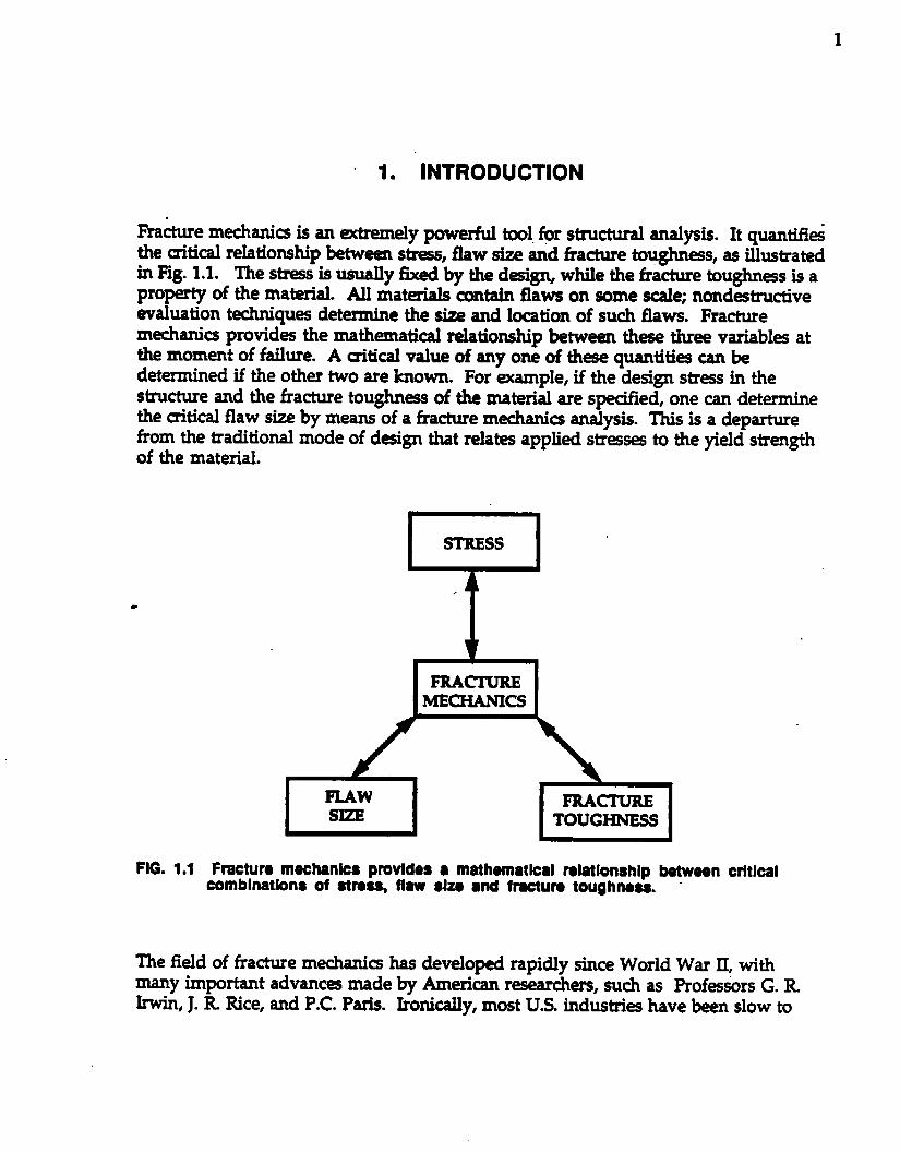
Fra&ure mechani= is an extremely pawerhd twl for structural analysis. It qwmtkthe uitical relationship ~tw~ s-, flaw size snd fracture toughn-s, as illustratedin Fig. 1.1. Thes- is usually &ed by the d~ign, while the fracture toughn~s is a

propertyof the matial. All materials contain flaws on some scale; nondestmctiveevaluation techniques determine the size and location of such flaws. Fracturemecharh provides the mathematical relationship between these three variables atthe moment of failure. A uitical value of any one of tke quantities can bedetermined if the other two are known. For ~ample, if the design stress in thestnacture and the fracture toughn~s of the material are specii%ed, one can determinethe critical flaw size by means of a fracture mechanics analysis. This is a departurefrom the traditional mode of design that relates applied str~ses to the yield strengthof the material.

I SruESs I

ImcruR.EMECHANICS I

FMw FucruRESIZE TOUGHNESS

FIG. 1.1 Fracturs muchank8 provides 8 math~atkal relationship between crltkalcombinations of straq flaw slza ●nd fmcture toughness. -

The field of fracture mechanh has developed rapidly since World War II, withmany important advanc~ made by American researchers, such as Profestirs G. RIrwin, J. R Rice, and P.C. Paris. Ironically, most U.S. industrk have been slow to

2

adopt the concepts of fracture medmni~, while their counterparts in Europe andJapan have embraced this technology with open arms. Where it has been applied,fracture mechani= has resulted not only in irmeased safety, but also in enormouseconomic knfits. For example, hundreds of millions of dolks have been roved inNorth Sea platform construction by basing weld flaw acceptance standards onfracture mechan.i~ a.nal~ (l).

U.S. industrial attempts to incorporate fracture mechanics technology have often “applied linear elastic fracture mechanb (LEFM), which is appropriate in someapplications but unsuitable for many others. With local or global plastic deformationin the structure, IX/FM can be extmrwly nonco~ative.

Elastic-plastic fracture mechanb should be applied in situations where LEFMisinvalid. Unfortunately, this technology is not well known to most U.S. industries.One exception is the nuclear power industry in the United States. Because of theirconcern for safety, electric utilities and government reguladng lmdi= have fundedextensive r-arch in elastic-plastic fracture mechanb over the past 20 years. Thiswork has produced well established procedures in the form of design handbmks,teting standards, and regulatory guid~. In addition, numerous articles have beenpublished in technical journals and COIifereIW proceedings.

Although the elastic-plastic fracture technology in the U.S. is fairly well advanced,much of it cannot be translated directly to industries other than nuclear power.Since nuclear reactors oprate at several hundred degrees above room temperature,the steal in these structur~ is on the upper shelf of toughness. More conventionalweIded steel structures, such as ships, bridg~, and pipelin~, operate at much lowertemperatur~, where the material may h in the ductil+brittle transition region. Inthis region, failure occurs by rapid, unstable cleavage fracture, but this tied brittlefracture is often preceded by signiikant of plastic deformation and ductile crackgrowth. Thus, fra-e in the transition region is elastic-plastic in nature, but theprocedur= developed by the nuclear power indus~ are intended to analyze ductilefracture on the upper shelf.

Considerable r-arch in elastic-plastic fracture in the ducti.lebrittle transition regionin the United Kingdom, driven largely by the development of oil resem~ in theNorth *a, has helped oil companies to build platforms lmth safely andeconomically. me design cdes and regulatory guide fof North Sea construction

contain requirements for fracture mechardm testing and analysis. Consequently, anumber of American oil companies with platforms in the North Sea are becomingfamilar with elastieplastic fracture technology.

In recmt years significant technolgy transfer among fracture mechani~ researchersin the U.S., Europe, and Japan has benefited all countries involved. For example, theanalys~ developed in Britain for the transition region have incorporated some ofthe advances that been made by the nuclear industry in the US. Jn addition,

3

researchers in the U.S. have begun to turn their attention to the transition region,primarily as a r-ult of interactions with rssea.rehem on the other side of the Atlantic.

Thus much of the fracture mecharii~ technology needed by U.S. industries thatconstruct and use welded steel structure is in place. llte problem is the availabilityof relevant information to engineers in th~ industris The details of fracturemechanb -tin% analysis, and application are scattered t@@out the publishedliterature. ..

This review attempts to define the state of the art in elastic-plastic fracturemechanim, as applied to welded steel structures The advantagw and shortcomingsof tiling approach are outlined, and pasible future directions are discussed.

. Information from a wide variety of r~urces is&&hukd. ‘The author hopes that thisreview will help to codify elastic-plastic fra~ mechanh so that it will gain morewid~read acceptance in industry.

Chapter 2 summarizes some of the fundamental concepts and basic assumptions offracture mechanics. This chapter sem~ as a framework for subsequent topi~; laterchapters refer back to the concepts in Chapter z Chapter 3 covers fracture toughrusstestin~ including standardized tests methods and newer test methods, such asfracture testing of welds. Recent research on data scatter and mack tip constraint isalso reviewed. Chapter 4 desai~ the application of fracture toughness data tod=ign, and mitiques the available methods, identifying the shortcomings of existingapproaches and making recommendations for future work. Chapter 5 summariz-the major points in the two previous chapters and gives the author’s pers~ctive onthe state of the art in elastic-plastic fracture mechartb.

2. FUNDAMENTAL CONCEPTS

Modem fracture mechani~ tram its ~ back Griflith (2), who h 1920 Ma.simple energy balance to predict the onset of fracture in brittle materials. ‘l’heGrifMt mmiel, with some moclMcations, is still applied today. An alternative butequivalent view of fracture considers the ~ and strains near the tip of the crack.Both of thae approach= are outlined Mow for the case of linear elastic materialbehavior. This is followed by an intrmiuction to elastic-plastic fracture mechanicsand a brief review of the micromechanisms of fracture in steels and weldments.

2.1 ENERGY APPROACH TO FRACTURE MECHANICS

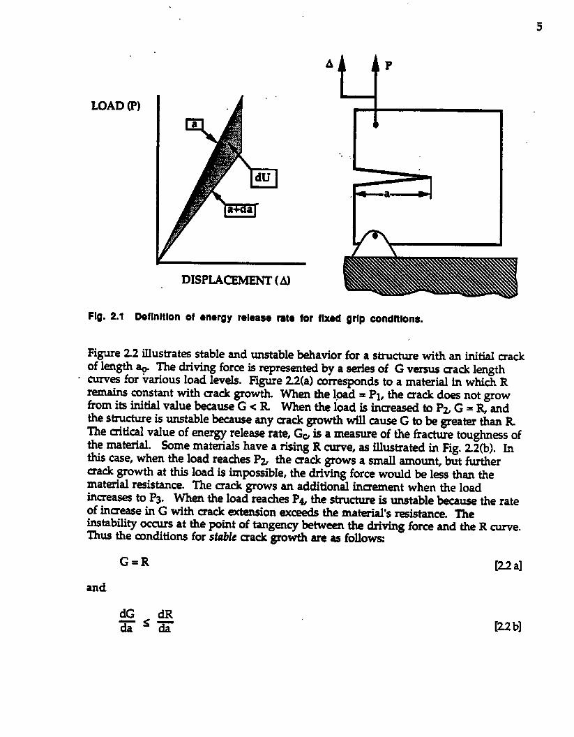
Consider a plate with a crack that is subjected to an external force, asillustrated in Fig. 21. The crack will grow when the energy available for crackextension is greater than or equal to the work required for crack growth.Stated another way, crack extension occurs when

driving force for fracture 2 material resistance.

This is essentially a restatement of the fu% law of thermodynamics. If the plate inFig. 21 is held at a fixed displacement, the conditions for crack advance are given by

where U is the elastic energy (per unit thickness) stored in the plate and W is thework required to grow the crack. Imzin (3) defined the term on the left of side of thisinequality as the energy release rate, G, and the term on the right as the materialresistance, R. Figure 2.1 illustra~ the energy release rate concept. If the ~ackextends an increment da under iixed grip conditions, the stored energy decreases bydU. For this inmemental mack extension to =cur, dU must be at least as large as dW,the work required to fracture the material and meate new surface.

If the driving force, G, is greater than the material resistance, ~ the crack extension isunstable. If G = ~ the crack growth may be.stable or unstable, depending on thematerial and Cofigu.ratiom When G and R are equal, stability depends on thesecond derivative of work, as discussed MOW.

5

f.LOAD (P)

DISPMCEMENT (A)

Au P

Fig. 2.1 Deflnltlon of .nergy releaso rat. for flxsd qrlp condltlon$.

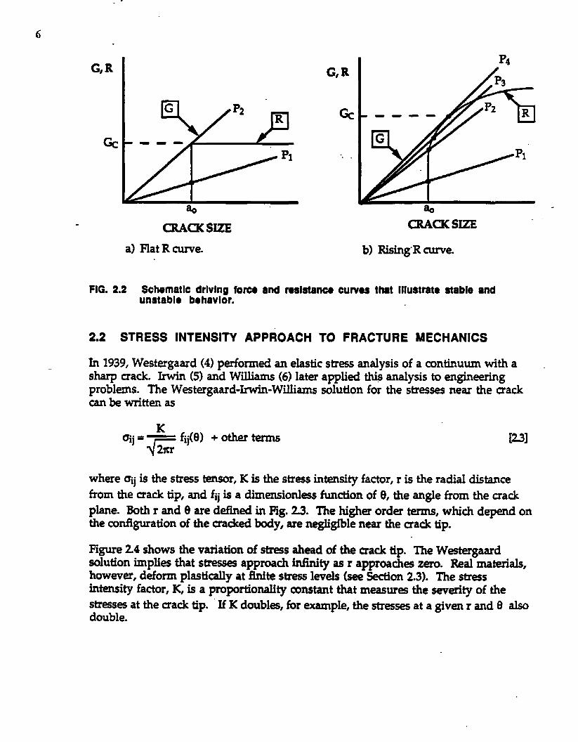
Figure 2.2 illustrates stable snd unstable behavior for a stmcture with an initial sackof length+ The driving force is represented by a series of G versus mack lengthcuwes for various load levels. Figure Z2(a) comesponds to a material in which Rremains constant with sack growth When the l+pad= PI, the crack does not growfrom its initial value because G < R When the load is increased to PZ G = R, andthe stnactu.re is unstable because any crack growth will cause G to be greater than RThe uitical value of energy release rate, Go is a measure of the fracture toughness ofthe material. Some materials have a rising R me, as illustrated in Fig. 22(b). Inthis case, when the load reaches Pa the sack grows a small amount, but furthermack growth at this load is impossible, the driving force would be less than thematerial resistance. The mack grows an additional increment when the loadirmeases to P3. When the load readws P~ the structure is unstable because the rateof inmease in G with mack extension exceeds the ma-s r~istance. Theinstability occurs at the point of tangen~ between the driving force and the R cume.~us the amditions for stile ffack growth areas follow

G=R [Z! a]

and

[22b)

CMCK SIZE

G, R

e

-. .

P4

,----

CMCK SIZE

a) Flat R cunm b) Rising”R curve.

FiG. 2.2 Sehem8tlc drlvlng form and reslstanco wives that Illustrate stable andunstable bthavlor.

2.2 STRESS INTENSITY APPROACH TO FRACTURE MECHANICS

h 1939, Westergaard (4) performed an elastic stress analysis of a continuum with asharp crack Irwin (5) and Williams (6) later applied this analysis to engineeringproblems. The Westergaard-Imin-Williarns solution for the stresses near the crackCanbewrittenas

K““-— fij(e) + OtheXt-t?,]-

F[u]

23cr

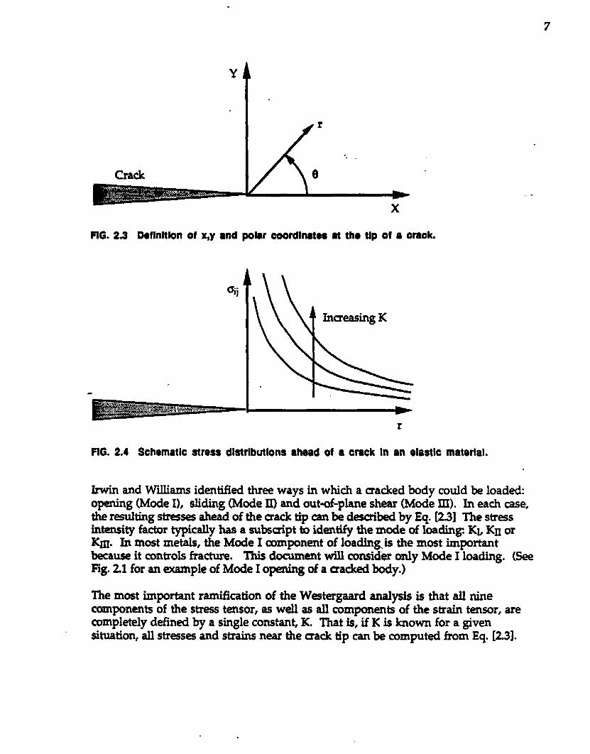
where dij iS the stress tensor, K iS the sties intensity factor, r is the radial distancefrom the sack tip, and fij is a d.imensionl=s function of e, the angle from the crackplane. Both r and 6 are dffied in 13g. 23. ‘l’he higher order terms, which depend onthe comllguration of the cracked lmdy, are negligible near the mack tip.

I%gure 24 shows the variation of str~s ahead of the crack tip. The Westergaardsolution implies that siresse approach inlin.ity as r approache zero. Real materials,however, deform plastically at finite stress levels (see Section 2.3). The str~sintensity factor, K, is a proportionality constant that measur~ the severity of thestresses at the crack tip. “If K double, for example, the stresses at a given r and e alsodouble.

Y

-. .,

crack

x

FIG. 2,2 Doflnltlon of x,y and polar coordlnataa atthotlp of a crack.

6j

r

FIG. 2.4 Schematic etreas dlatrlbutlons ●head of a crack In an elaetlc rnaterlal.

lwin and Williams identified thr- ways in which a sacked body could h loaded:opening (Mode I), sliding (Mode II) and outd-plane shear (Mode III). In each case,the resuliing stm- ahead of the crack tip can& d~uilwd by Eq. [23] The str~sintensity factor typically has a subsaipt to identify the mde of loadin~ KL KU orKm. In most metals, the Mode I uxnponent of loading.is the most ixnprtantbecau.w it controls fracture. This document will consid~ only Mode I loading. (SeeHg. 21 for an aunple of Mtie I opning of a sacked kxiy.)

The most important ramikation of the Westergaard analysis is that all nineComponwits of the sixess tensor, as well as all components of the strain tensor, arecompletely deflried by a single constant, K ‘l%at is, if K is known for a givensituation, all stresses and strains near the sack tip can be computed from Eq. [23].

8

Consider a small element of material at the crack tip. It is reasonable to assume thatthis material element fails when it qwrience a mitical combination of stress andstiaim Thus, this material element must fail at a uitical K value. This philosophyled to the definition of a critical str=s intity, KIG at the onset of mack extension(7).

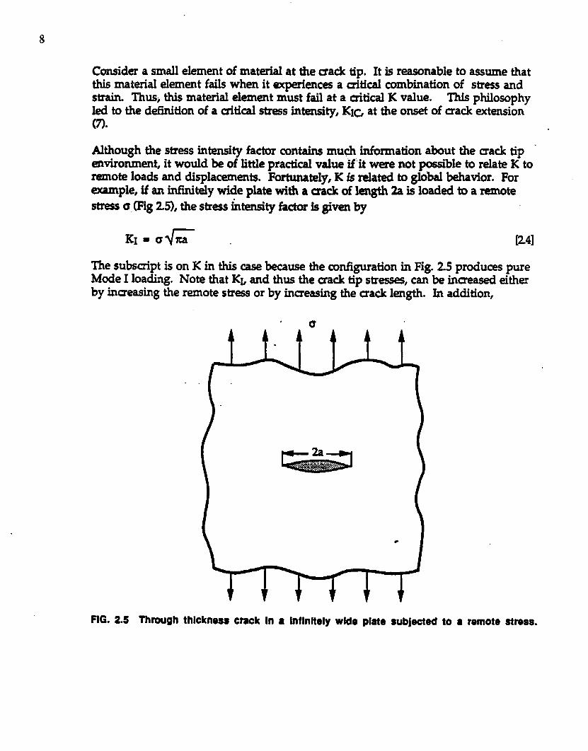
Although the stress intensity factor contains much information alwut the sack tip -environment, it would be of little practical value if it were not possible to relate K toremote loads and displacements. Fortunately, K is related to global bhatior. Forexaxnple, if an infinitely wide plate with a crack of length 2a is loaded to a remotestms 0 (Fig M), the str~s &nsity factor is given by

The subsdpt is on K in this case because the cordiguration in Fig. 25 produces pureMtie I loading. Note that Kb and thus the crack tip str~, can be increased eitherby inmeasing the remote stress or by inaeasing the crack length. In addition,

FIG. 2.5 Through thickness Crack In ● Inflnltely wide plate subjscted to a remote stress.

9

by setting K1 to the critical value for the material, it is possible to relate stress, fracturetoughnes ~IC), and dtical mack size

Equation [24] applies only to a through-thiclm~ mack in an Mnite plate; i.e., aplate whose width is>> 2a. For other amfigurations, K1an be writ&II in thefollowing form.

lx]

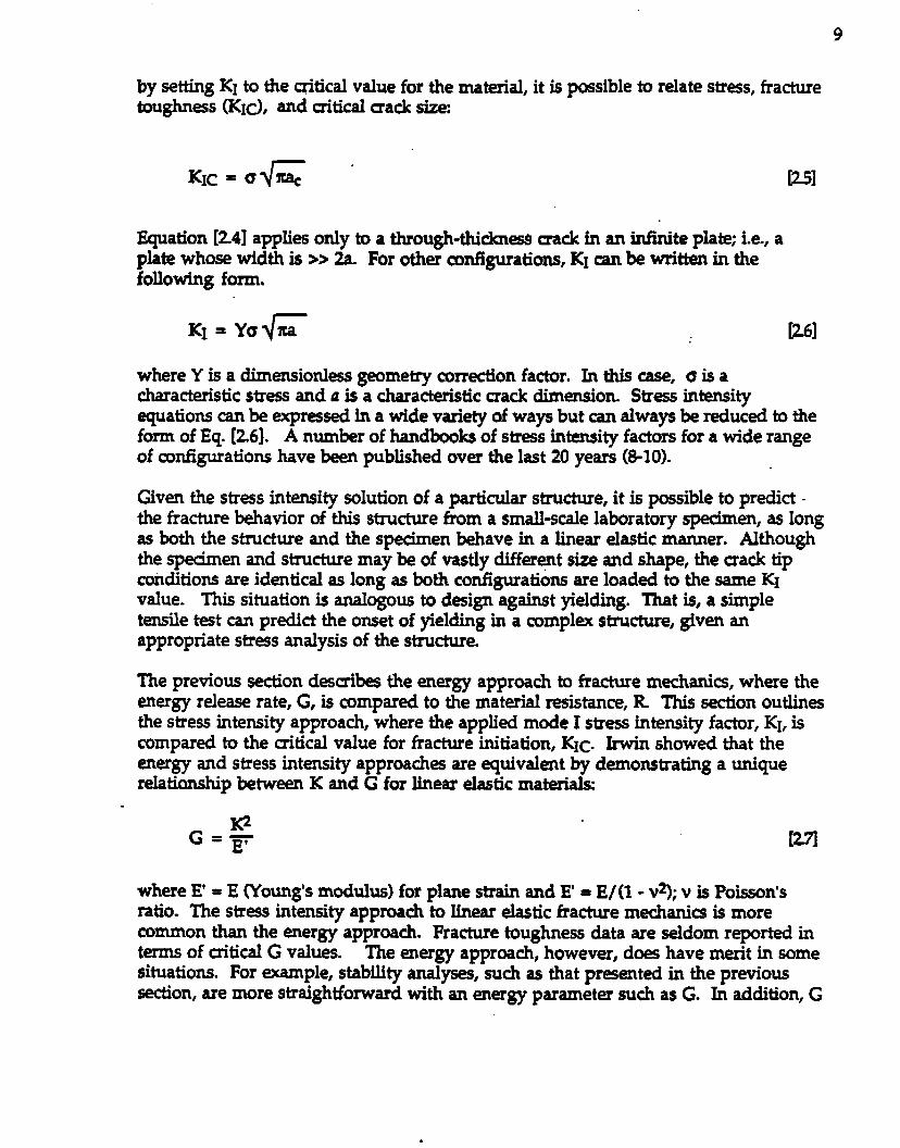
where Y is a dimensions geometry correction factor. In this case, o is acharacteristic stress and a is a charact~tic mack dim-ion. %r- intensityequations can be ~resed in a wide variety of ways but can always be reduced to theform of Eq. [2.6]. A num?xr of handlmoks of stress intensity factors for a wide rangeof cotigwrations have been published over the last 20 years (8-10).

Given the stress intensity solution of a particular structure, it is possible to predict -the fracture behavior of this structure from a small-scale laboratory spedmen, as longas both the stmcture and the specimen behave in a linear elastic manner. Althoughthe spedmen and structure maybe of vastly different size and shape, the crack tipconditions are identical as long as both configurations are loaded to the same K1value. This situation is analogous to design against yielding. That is, a simpletensile test can predict the onset of yielding in a compk structure, given anappropriate stress analysis of the structure.

The previous section d~cribes the energy approach to fracture mechanics, where theaergy release rate, G, is compared to the material resistance, ~ This section outlinesthe stress intensity approach, where the applied mode I stress intensity factor, KI, iscompared to the critical value for fracture initiation, KIc. hvin showed that theenergy and stress intensity approaches are equivalent by demonstrating a uniquerelationship between K and G for linear elastic materials

VI

where E’ = E (Young’s modulus) for plane strain and E = E/(1 - v2); v is Poisson’sratio. The stress intensity approach to linear elastic fracture mechani~ is morecommon than the energy approadi. Fracture toughness data are seldom reprted interms of uitical G values. The energy approach, however, does have merit in somesituations. For mple, stability analyses, such as that pr~ented in the previoussection, are more straightfonmrd with an energy parameter such as G. In addition, G

is more convenient than K in mixed mode problems because G components areadditive:

Gto~ = GI+Gu+Gm

but

All of the above analyses are stictly valid only for isotropic materials that behave ina prfectly linear elastic manner. when there is a small amount of plasticdeformation at the tip of the cra~ linear elastic fracture mechard~ @FM) giv~ agmd approximation of actual material Mhavior. Eventually, however, the tlwrybreak down. The following section d~cribes the limitations of LEFM and the-ting methods to account for crack tip plasticity.

2.3 ELASTIC-PLASTIC FRACTURE MECHANICS

Fracture mechanics approaches to crack tip plasticity fall into two main categories: 1)simple corrections to LEFM theory, and 2) fracture parameters which allow fornonlinear material behavior. Irwin (11) proposed a simple plastic zone correction to .the stress intensity factor. An alternative plastic zone correction was developed byDugdale (12) and Barenblatt (13). The fist truly elastic-plastic frame parameter, thesack tip opening displacement (CTOD), was proposed by Wells (14) in 1%1. Severalyears later, Rice (15) developed the J mntour integral, a parameter that approximate= -elastic-plastic deformation with a nonlinear elastic material assumption. The Jintegral can be viewed as both an energy parameter and a stress intensity-likequantity. In addition, J is uniquely related to CCOD under certain conditions.

2.3.1 IMn Plastic Zone Correction

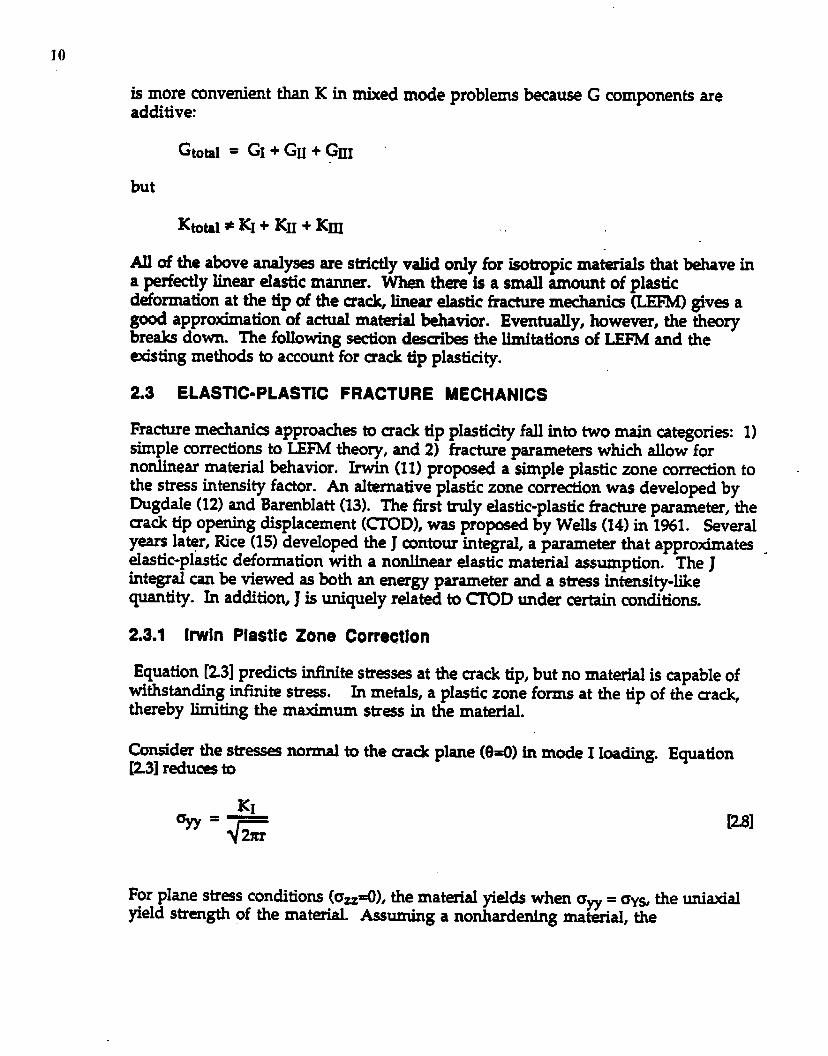
Equation [23] predicts inhite stresses at the crack tip, but no material is capable ofwithstanding ir&.ite stress. In metals, a plastic zone forms at the tip of the sack,thereby limiting the maximum str~ in the material.

Consider the slresse normal to the crack plane (e=O) in mode I loading. Equation[23] redu~ to

D1

For plane stress conditions (on=O), the material yields when crm = ~ys, the uniaxialyield strength of the material. Assuming a nonhardening material, the

11

% bA

ms

r

FIG. 2.6 First order ●stimate of plastic zone size for plan. stress conditions.

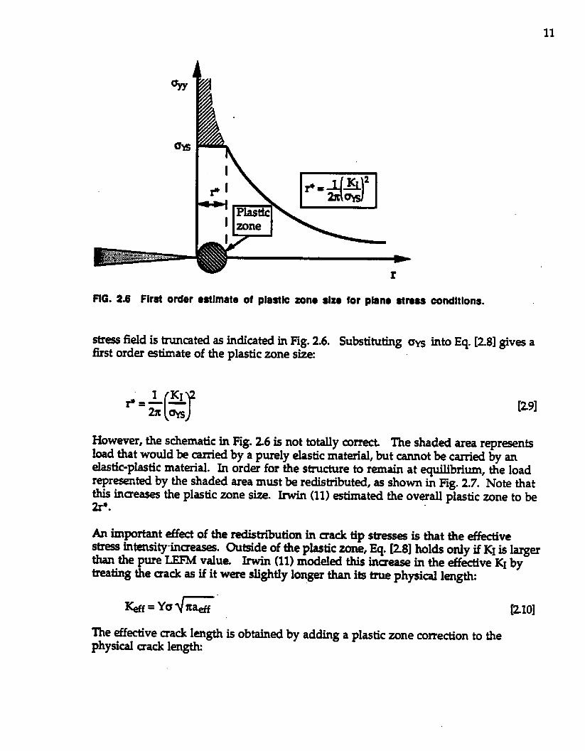
stress fieId is truncated as indicated in Hg. 2.6. Substituting an into Eq. [2.8] gives afist order estimate of the plastic zone size

[29]

However, the schematic in Fig. 26 is not totally corr- The shaded area representsload that would be camied by a purely elastic material, but cannot be carried by anelastic-plastic material. In order for the structure to remain at equilibrium, the loadrepr~ted by the shaded area must be redistributed, as shown in Fig. 2.7. Note thatthis increases the plastic zone size. Invin (11) estimated the overall plastic zone to be2r*.

An imprtant effect of the redistribution in mac.k tip stresses is that the effectivestress intensity-incre=. Outside of the plastic zone, Eq. [28] holds only if KI is largerthan the pure LEFM value = (11) modeled this inme~ in the effective K1bytreating the sack as if it were slightly longer than its tie physical Iengtk

&ff=Yal/” 210]

The effective mack Iength is obtained by adding a plastic zone correction to thephysical crack lengtlc

12

r

FIG. 2.7 Irwin plastic

+2F4

~=a+rY

~=a+rY

zono corrsotlon for plan. stress conditions.

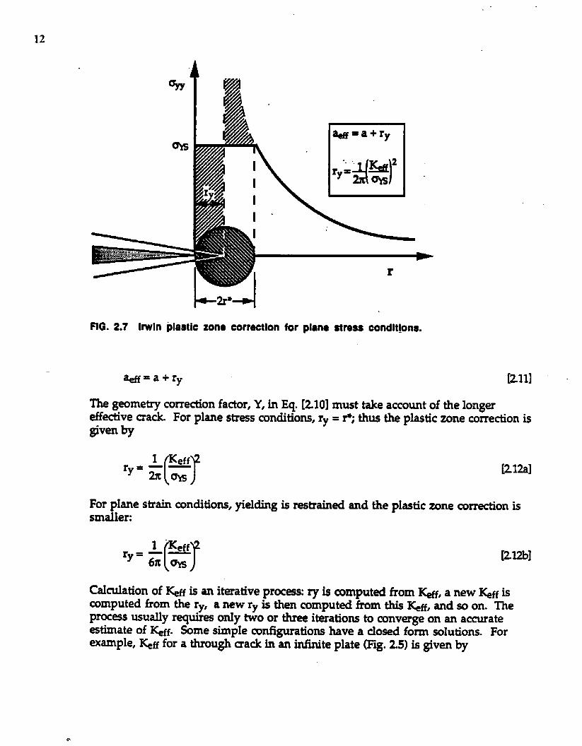
ml]

The geometry correction factor, Y, in Eq. [Z1O] must take account of the longereffective mack. For plane stress conditions, rY = P; thus the plastic zone correction is@V~ by

[212a]

For plane strain conditions, yielding is restrained and the plastic zone mrrection issmalle~

1 - ~ff

rr

——‘y= 6X ~

[2Ub]

Calculation of &ff is an iterative process ry is computed from ~, a new &ff iscomputed from the ry, a new ry is then computed from this &ff, and so on. Theprocess usually requires only two or three iterations to converge on an accurateestimate of &ff. Some simple cotigurations have a closed form solutions. Forexample, &ff for a through sack in an inhite plate (Fig. 25) is given by

13

B13]

2.3.2 Strip Yield Plastic Zone CorrectIon

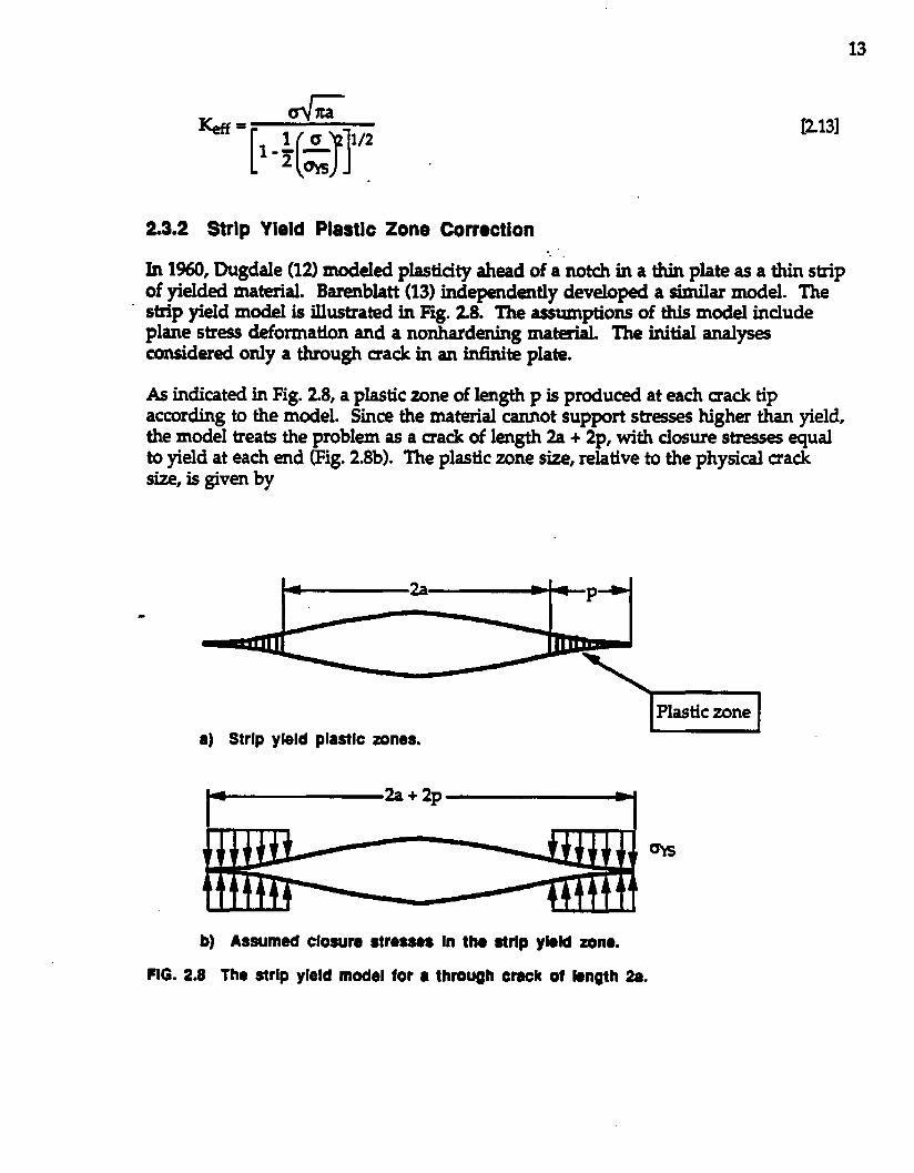
In 1%0, Dttgdale (12) modeled plastiaty ahead of a notch in a b plate as a thin stripof yielded material. Barenblati (13) independently developed a similar model. The

- sfrip yield model is illustrated in Fig. 28. The emunpticms of this model includeplane stress deformation and a norihardening material. The initial analysescmsidered only a through mack in an Mn.ite plate.

As indicated in Fig. 2.8, a plastic zone of length p is produced at each crack tipaccording to the model. Since the material cannot support straes higher than yield,the model treats the problem as a mack of length 2a + 2p, with closure str~ses equalto yield at each end (Fig. 2.8b). The plastic zone size, relative to the physical crack&, is gh~ by

a) Strip yield plastic zones.

b) Assumed closure stresses [n tho strip yfald zorm.

FIG. 2.8 The atrlp yl@ldmodel for ● through craok of length 2a.

p14]

IfM is taken as (a + p), the effective KI is given by

@15J

Howwer, this equation leads to overestima~ of ~ because closure str~ causethe true effective mack length to b somewhat less than (a + p). Burdenkin andStone a.nal~ the sixip yield model further and dtived a more appropriaterelationship for ~.

[216]

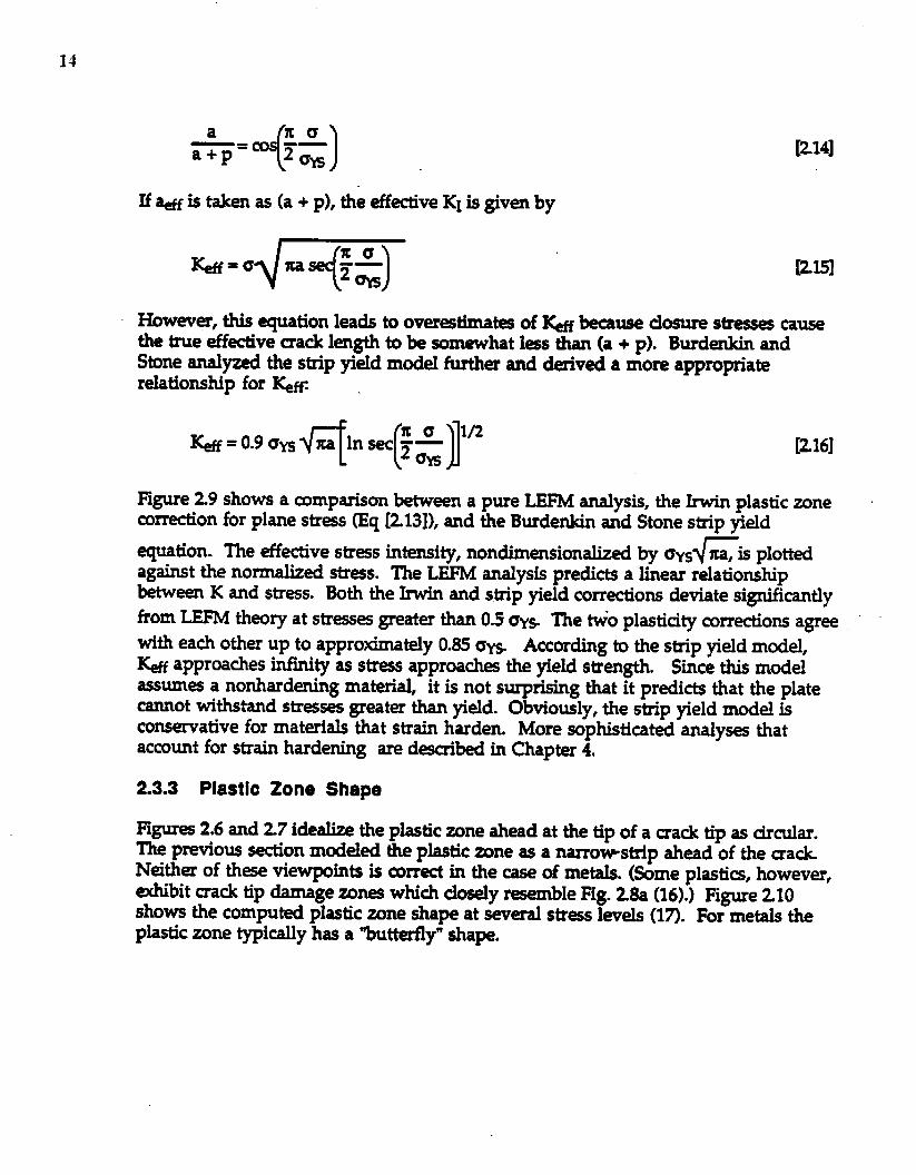
figure 29 shows a comparison between a pure LEFh4 analysis, the Imvin plastic zonecorrection for plane strss (Eq [213]), and the Burdexikin and Stone strip yield

vequation. The effective stress intensity, nondimmsionalized by crys ma,is plottedagainst the normalized str~s. The LEFM analysis predicts a linear relationshipbetween K and stress. Both the Irwin and strip yield corrections deviate significantlyfrom LEFM theory at stress greater than 0.5 ~s. The ~“o plastiaty corrections agreewith each other up to approximately 0.85 *s. According to the strip yield model,& appr~~es infinity as stress approaches the yield strength Since this modelassumes a nonhardening material, it is not surprising that it predicts that the platecannot withstand stresses greater than yield. Obviously, the strip yield model iscons-ative for materials that strain harden. More sophisticated analy~ thataccount for strain hardening are described in Chapter 4.

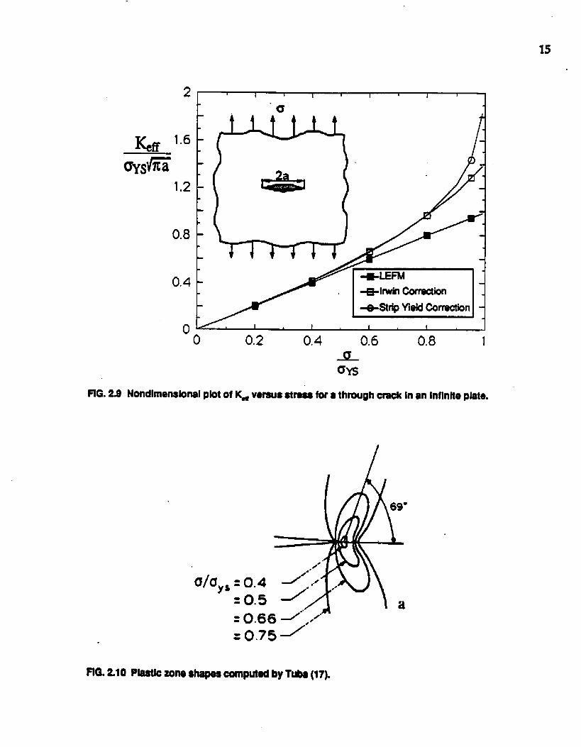
2.3.3 Plastic Zone Shape

H- 2.6 and 27 idealize the plastic zone ahead at the tip of a mack tip as drcular.The previous section modeled the plastic zone as a narrcwstrip ahead of the mackNeither of th~e viewpints is mrrect in the case of metals. (Some plastics, however,exhibit crack tip damage zons which closely ~ble 13g. 28a (16).) Figure 210shows the computed plastic zone shape at several str~s levels (17). For metals theplastic =ne typically has a “butterfly” shap.

15

flG. 2.2

2 I I I i 1 Ia /

.6 -

,2 -

0.8 -

0.4 -

r

OF’ I I I 1

0 0.2 0.4 0.6 0.8 1

o%

Nondlmenslonalplot of Kwvemus stress for ● throughcrack In an Inflntteplate.

~G. 2.10 MSUCzone $hapeeCOMPUttiby T- (17).

16

2.3.4 Crack Tip Openhg Displacement

In the late 1950s, Wells attempted to apply Invin’s str-s intensity mncept tomeasure the fracture tough.rws of a series of medium strength structural steels. Hefound that t.lwe materials kxhibited a high degree of plastic deformation prior tofracture. This was gcmd news from a d-ign engineer’s standpoint because itindicated high toughness in th- steels. However, signihnt plastiaty was bad .news for theoretiaans because it meant that linear elastic fracture mechanb was notapplicable to typical structural steels.

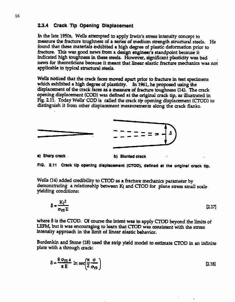
Wells noticed that the uack faces moved apart prior to fracture in -t specimenswhich exhibited a high d-of plastidy. In 1%1, he propsed using thedisplacement of the =ack fa~ as a measure of fracture toughn~s (14). The mackopening displacement (COD) was defied at the original crack tip, as illustrated inFig. 211. Today Wells’ COD is called the uack tip opening displacement (CTOD) todistinguish it from other displacement measurements along the sack flanks.

A----9-

= - .8-m ---0

a) Sharp cniick b) Bluntsdcrook

FIG. 2.11 Crack tlp opanlng dlsplacemtnt (CTOD), doflnad at tho orlglnal crack tip.

WeIls (14) added credibility to CTOD as a fracture mechani~ parameter bydemonstrating a relationship between KI and ~OD for plane stress small scaleyielding conditions:

where 5 is the ~D. Of murse the intent was to apply ~D &yond the limits ofLEFM, but it was encouraging to learn that ~OD was consistent with the stressintensity approach in the limit of linear elastic behavior.

Burderddn and Stone (18) used the strip yield model to estimate mOD in an iniiniteplate with a through maclc

[218]

Series expansion of the in sec term yields

[219a]

Thus when G/CfYS is small, the Burdekin and Stone equation reduces to the Wellsrelationship for small scale yielding (Eq. [217J).

2.3.5 The J Contour Integral

Plasticity th=ry is more complex than the theory of elastiaty. When a materialdeforms elastically, it is possible to deduce the m.umnt stresses from the currentstrains, and vice versa. However, material r~ponse to plastic deformation is historydependen~ Since a set of plastic strains d- not uniquely define the stresses in thematerial, a closed-fomn solution to the crack tip str~s field, similar to theWestergaard solution for linear elastic materials, is not possible for an elastic-plasticmaterial.

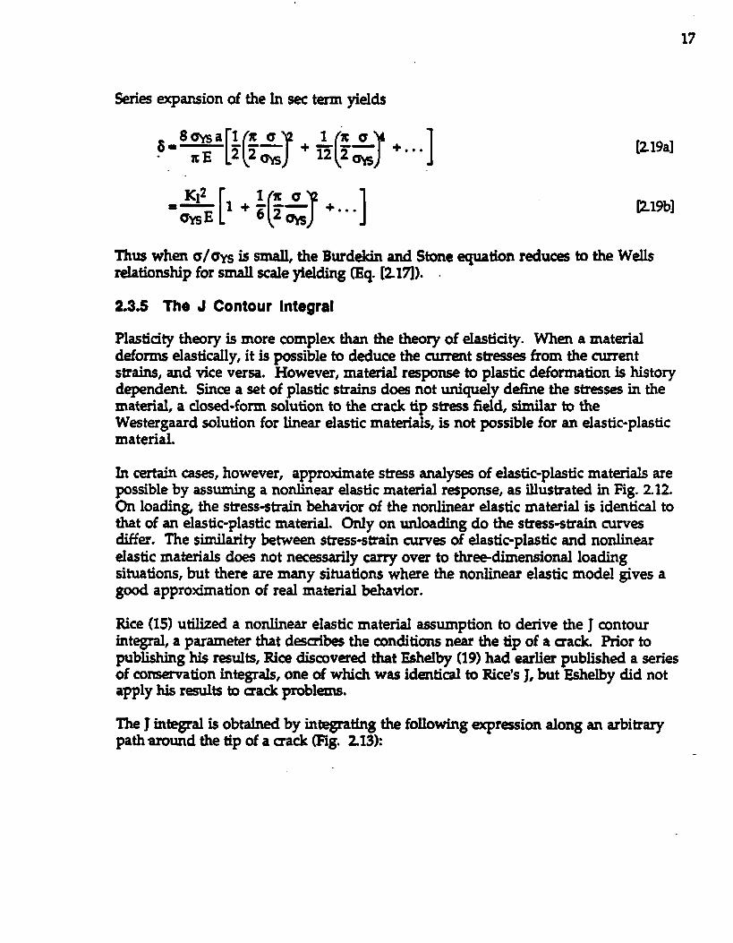
In certain cases, however, approximate str~s analyses of elastic-plastic materials arepossible by assuming a nonlinear elastic material r~ponse, as illustrated in Fig. 212.On load.in& the stress-strain behavior of the nonlinear elastic material is identical tothat of an elastic-plastic material. Only on unloading do the stress-strain cumesdiffer. The similarity between stress-strain cum= of elastic-plsstic and nonlinearelastic materisls d- not nec~sarily carry over to thr~dimensional loadingsituations, but there are many situations where the nonlinear elastic model gives agood approximation of real material behavior.

Rice (15) utilized a nonlinesr elastic material assumption to derive the J contourintegral, a parameter that d=ccibes the conditions near the tip of a crack Prior topublishing his r~ults, Rice discovered that Esheby (19) had earlier published a seriesof comemation integrals, one of which was identical to Rice’s J, but Eshelby did notapply his rendts to tack problems.

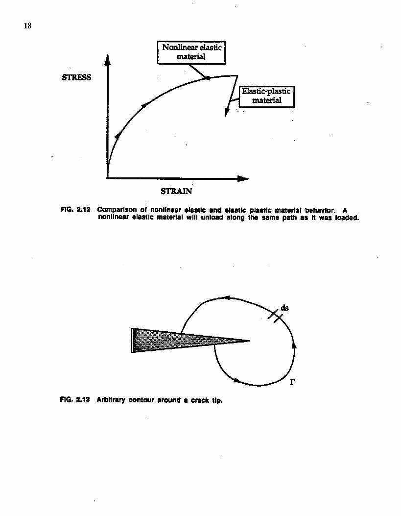
The J integral is obtained by integrating the following qression along an arbitrarypath around the tip of a aaclc @lg. 213):

1,8

STREss

/

FIG. 2.12 Comparison of nonlinear ●laatlc snd ●lastlc plastlc material behavior. Anonlinear elaatlc material wIII unload along the same p8th as It was loaded.

FIG. 2.13 Arbttrary contour ●tound ● craok tip.

19

ml

where r is the path of integration, W is the strain energy density, T is the traction-r, u is the displacement vector, and ds is an-increment along r. The coordinat~x and y areas defuwd in Fig. 23. For nonlinear elastic materials; Rice showed thatthe value of J is independent of the integration path as long as the amtour enclosesthe mack tip, as illustrated in Hg. 213.

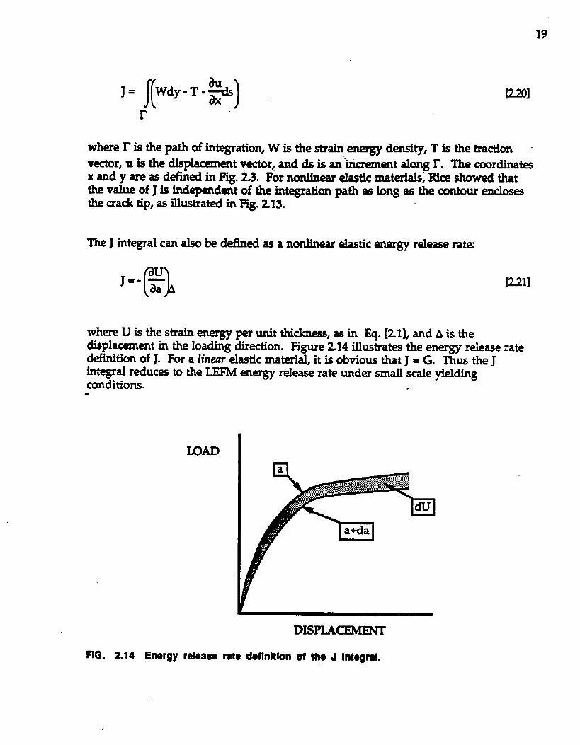
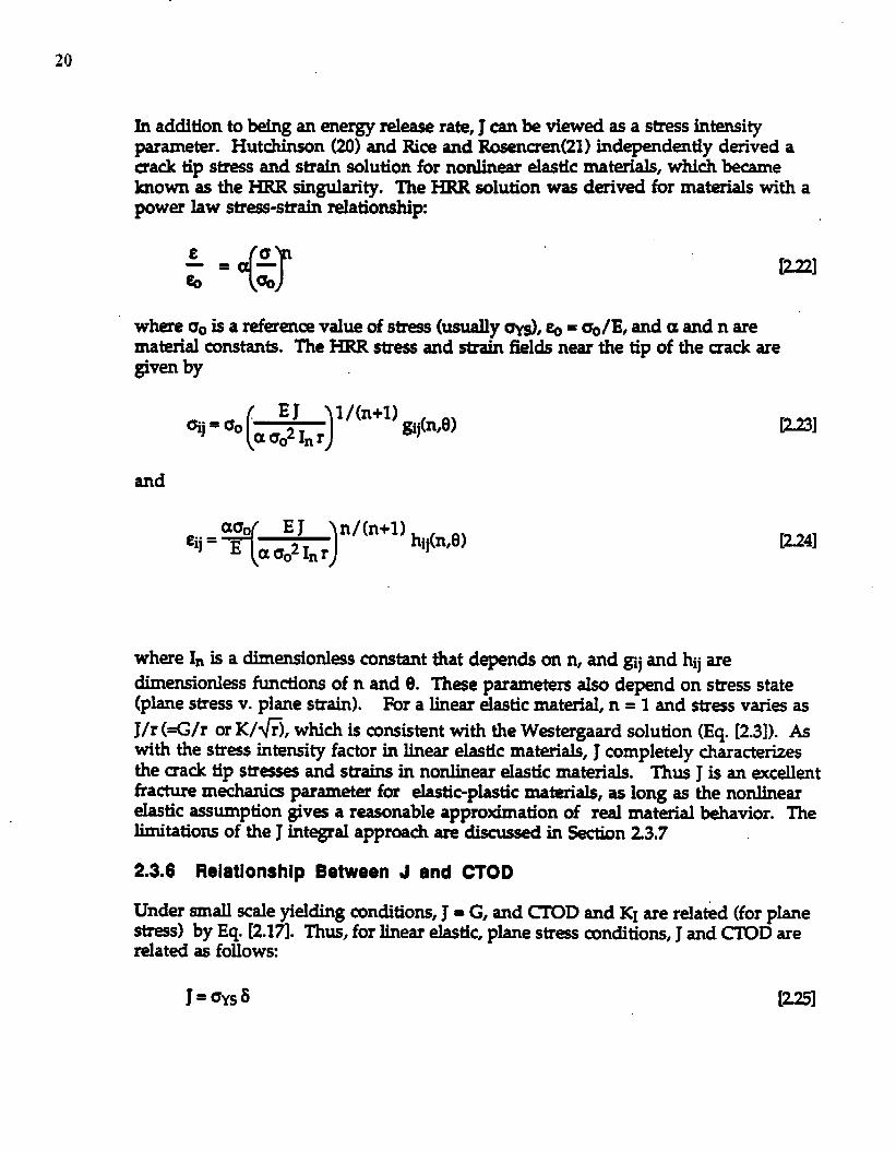
The J integral can also be defined as a nonlinear elastic energy release rate

where U is the strain energy per unit thickness, as in Eq. [21], and A is thedisplacement in the loading direction. F@re 2.14 illustrates the energy release ratedefinition of J. For a linear elastic material, it is obvious that J = G. Thus the Jintegral reduces to the LEFM energy release rate under small scale yieldingconditions.

LOAD

DISPMCEMENT

FIG. 2.14 Energy releaea rate definition of tho J Integral.

20

In addition to being an energy relesse rate, J can IM viewed as a stress intensityparameter. Hut&inson (20) and Rice and Rosencren(21) independently derived acrack tip stress and strain solution for nonlinear elastic materials, which becamehewn as the HRR singularity. The HRR solution was derived for materials withpower law stress-strain relationship

a

ml

where co is a reference value ofs- (usually @, @ = Go/E, and u and n arematerial constants. The HRR stress and strain @ids near the tip of the crack are@Ven by

and

‘ij=w*)n’(n+l)hi’(n”)

u]

where In is a dimensionless constant that depends on n, ad gij ad hij are

dimensionl=s functions of n and 0. Th~e parameters also depend on stress state(plane stress v. plane strain). For a linear elastic material, n = 1 snd stress varies as

J/r (=G/r m K/$), wNch i$ mn$ktent with the w-t~gaard solution (Eq. [2.3]). &with the str-s intensity factor in linear elastic materials, J completely characterizesthe crack tip str~ and strsins in nonlinear elastic materials. Thus J is an ~cellentfracture mechani~ parameter for elastic-plastic materials, as long as the nonlinearelastic assumption give a reasonable approximation of reaI material behavior. Thelimitations of the J integral approach are discussed in Section 23.7

2.3.6 Relationship Between J and CTOD

Under small scale yielding conditions, J = G, and CI’OD and K1 are related (for phnestress) by Eq. [2.17]. Thus, for linear elastic, plane str~ conditions, J and CIUD arerelated as follows

21

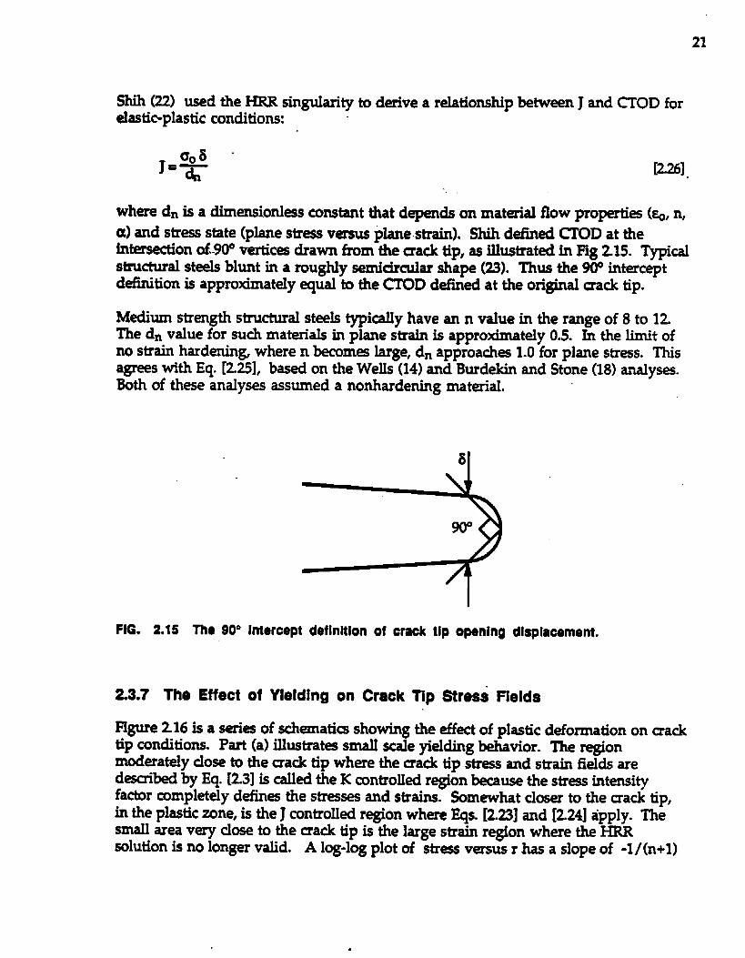
Shih (22) used the HRR singularity to derive a relationship be~een J and CTOD forelastic-plastic conditions: “

#ff8 -w].

where dn is a dimensionless constant that depends on material flow pro-= (b, n,a) and stress state (plane stress ve.raus plane. strain). Shih defined CTOD at theintersecdon of..9~ vertices drawn from the sack tip, as illustrated in Flg 215. Typicalstructural steels blunt in a roughly semicircular shape (23). Thus the 90° interceptdefinition is approximately equal to the CITID defuwd at the original sack tip.

Wdhun strength structural steels typimlly have an n value in the range of 8 to 12.The dn value for such materials in plane strain is approximately 0.5. In the limit ofno strain hardenin~ where n &coma large, dn approach- 1.0 for plane stress. Thisagrees with Eq. [225], based on the Wells (14) and Bu.rdek.inand Stone (18) analvses.B&h of these analyses assumed a nonhardening material.

8

90°

FIG. 2.15 The 90° Intercept definition of crack tip opening dlaplacement.

.

2.3.7 Th@ Effect of Yleldlng on Crack Tip Stress Fields

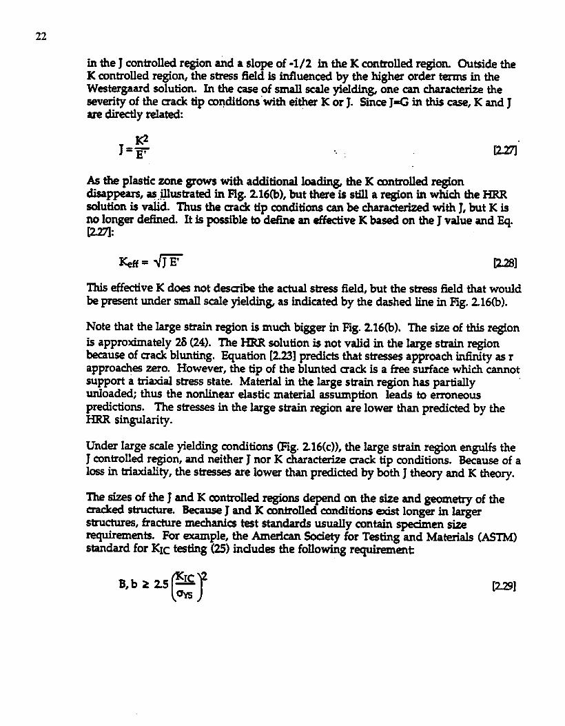
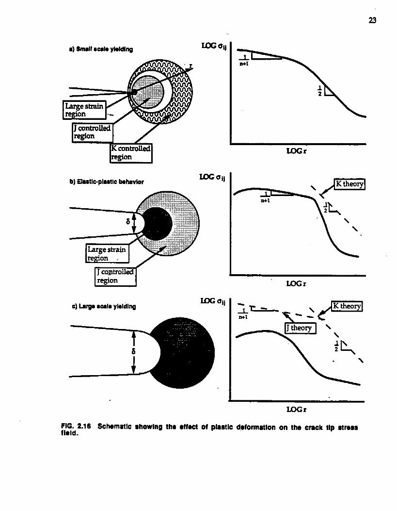
l@re 216 is a seri~ of schemati= showing the effect of plastic deformation on ~acktip conditions. Part (a] illustrates small scale yielding bhavior. ‘l’he regionmoderately close to the crack tip where the mack tip str- and strain fields ared-bed by Eq. [23] is called the K controlled region because the stress intensityfactor completely defin= the str~ses and strains. Somewhat closer to the mack tip,in the plastic zone, is the J controlled region where Eqs. [2.23] and [2.24] apply. Thesmall area very close to the mack tip is the large strain region where the HRRsolution is no longer valid. A log-log plot of stress versus r has a slope of -1 /(n+l)

22

in the J controlled region and a slope of -1/2 in the K controlled region. Outside theK controlled region, the stress field is influenced by the high= order terms in theWest=gaard solution. In the case of small scale yieldin~ one can characterize theseverity of the cra& tip conditions ”with either K or J. Since J=G in this case, K and Jare directly related:

wl-

A the pIastic zone grows with additional loadin~ the K controlled regiondisappears, m+illusfrated in F3g. 216(b), but there is still a region in which the HRRsolution is valid. Thus the crack tip conditions can be characterized with J, but K isno longer defined. It is possible to detine an effective K based on the J value and Eq.m

&ff=llmThis effective K does not describe the actual stress field, but the stress field that wouldbe present under d scale yieldin~ as indicated by the dashed line in Hg. 216(b).

Note that the large strain region is much bigger in Fig. Z16(b). The size of this regionis approximately 26 (24). The HRR solution is not valid in the large strain regionbecause of mack blunting. Equation [223] predicts that stresses approach infinity as rapproaches zero. However, the tip of the blunted crack is a free surface which cannotsupport a triaxial stress state. Material in the large strain region has partiallyunloaded; thus the nonlinear elastic material assumption leads to erroneouspredictions. The stresses in the large strain region are lower than predicted by theHRR singularity.

Under Iarge scale yielding conditions (Fig. 216(c)), the large strain region engulfs theJ controlled region, and neither J nor K characterize crack tip conditions. Because of aloss in triaxiality, the str=ses are lower than predicted by both J theory and K theory.

The sizes of the J and K controlled regions depend on the size and geometry of the-ed structure. Because J and K controlled conditions tit longer in largerstructures, fracture me&mis test standards usually contain spedrnen sizerequirements. For example, the American %ciety for Tding and Materials (ASTM)standard for KXCtd.ng (25) indudm the following requirement

[m]

●) Small scslo ykldiq

b)Ela8tlc-plastlcbol!wior

EiEr

Lm qj

LOGr

Lm eq

c)L8rgo8c,I*ylddlngm Uij

. dKtheon4

“\ \ \

LOGr

LOGr

FIG. 2.16 Schomatlc showing ths ●ffect of plastlc d.efonnatlon on the crock tlp stressfield.

24

.

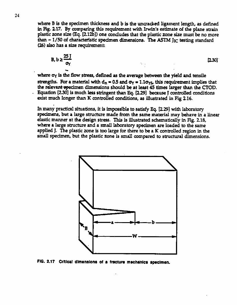
where B is the spedrnen thickness and b is the untracked ligament length, as defiedin Fig. 217. By comparing this requirement with Iwin’s estimate of the plane strainplastic zone size @q. [212b]) one concludes that the plastic zone size must&no morethan - 1/50 of characteristic spedmen dimensions. me ~ JIC tating standard(26) also has a size requirement

B,b2q*

E301”-.

*

where ay is the flow stress, dei?med as the average between the yield and tensilestrengths. Fdr a material with dn = 03 and w = 1.1- this requirement impli~ thatthe relevant-en dimensions should beat least 45 tires larger than the ~OD.Equation [230] is much hs stringent than Eq. [~9] kause J controlled conditionsexist much longer than K controlled conditions, as illustrated in Fig 216.

In many practical situations, it is impossible to satisfy Eq. [229] with laboratoryspecimens, bwt a large structure made from the ssme material may behave in a linearelsstic manner at the d~ign stress. This is illustrated schematically in Fig. 2.18,where a large structure snd a small laboratory specimen are loaded to the sameapplied J. The plastic zone is too large for there to be a K controlled region in thesmall specimen, but the plastic zone is small compared to stnxtural dimensions.

< a -. ,4 b~‘B

- w~

FIG. 2.17 Crltlcal dimensions of & fracture mecha-nlcs specimen.

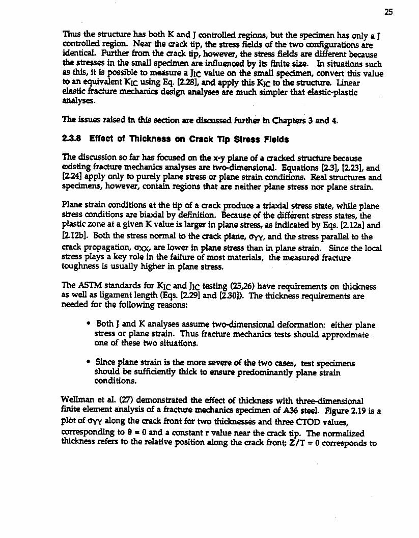
Thus the structure has lmth K and J controlled regions, but the specimen has only a Jcontrolled region. Near the uack tip, the str~ fields of the two configurations areidenticaI. Further from the crack tip, however, the stress fields are different becausethe stresses in the small specimen are i.nfluend by its bite size. In situatiom SU&

as this, it is possible to measure a JIC value on the small specimen, convm this valueto an equivalent KIC using Eq. [22$], and apply this KIc to the stmcture. Linearelastic fracture mechanics deign analyses are much simpler that elastic-plastic .analyw.

2.3.8 Effect of Thfckness on Crsck Tlp Stress Fields

The discussion so far has focused on the x-y plane of a sacked stnacture becauseexisting fracture mechanics analyses are tw~en,sional. Equations [Z3], [2.23], and[2241 apply o~y topurelyplane stressor plane strain conditions. Red StIUtieS ~dspedxrmns, however, contain regions that are neither plane stress nor plsne strak

PIsne strain renditions at the tip of a ffack produce a triaxial stress state, while planestress conditions are biaxial by dei?nition. Because of the difkrent stress states, theplastic zone at a given K value is larger in pkme stress, as indicated by Eqs. [212a] and

[212bl. Both tie stms normal to the crack plane, ~, and the str=s parallel to the=ack propagation, ~ are lower in plane str~ than in plane strain. Since the localstress plays a key role in the faihre of most materials, the measured fracturetoughness is usually higher in plane sties.

The ASTM standards for KIC and JIC testing (2526) have requirements on thicknessas well as ligament length (Eqs. [229] and [2.30]). The thickrws requiremm~ aren~ed for the following reasons:

● Both J and K analyses assume two-dimensional deformation either planestress or plane strain. Thus fracture mechanb tests should approximate .one of these two situations.

● Since plane strain is the more severe of the two cases, tat specimensshould be suffiaently thick to ensure predominanttly plane strainconditions.

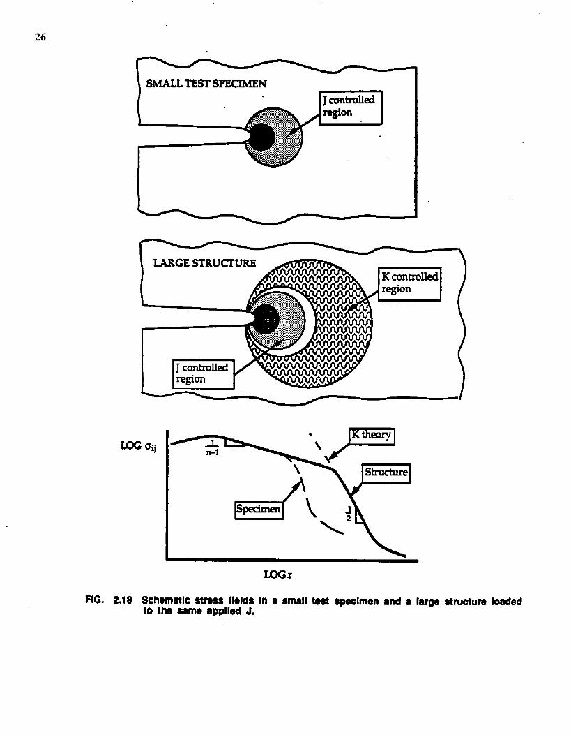
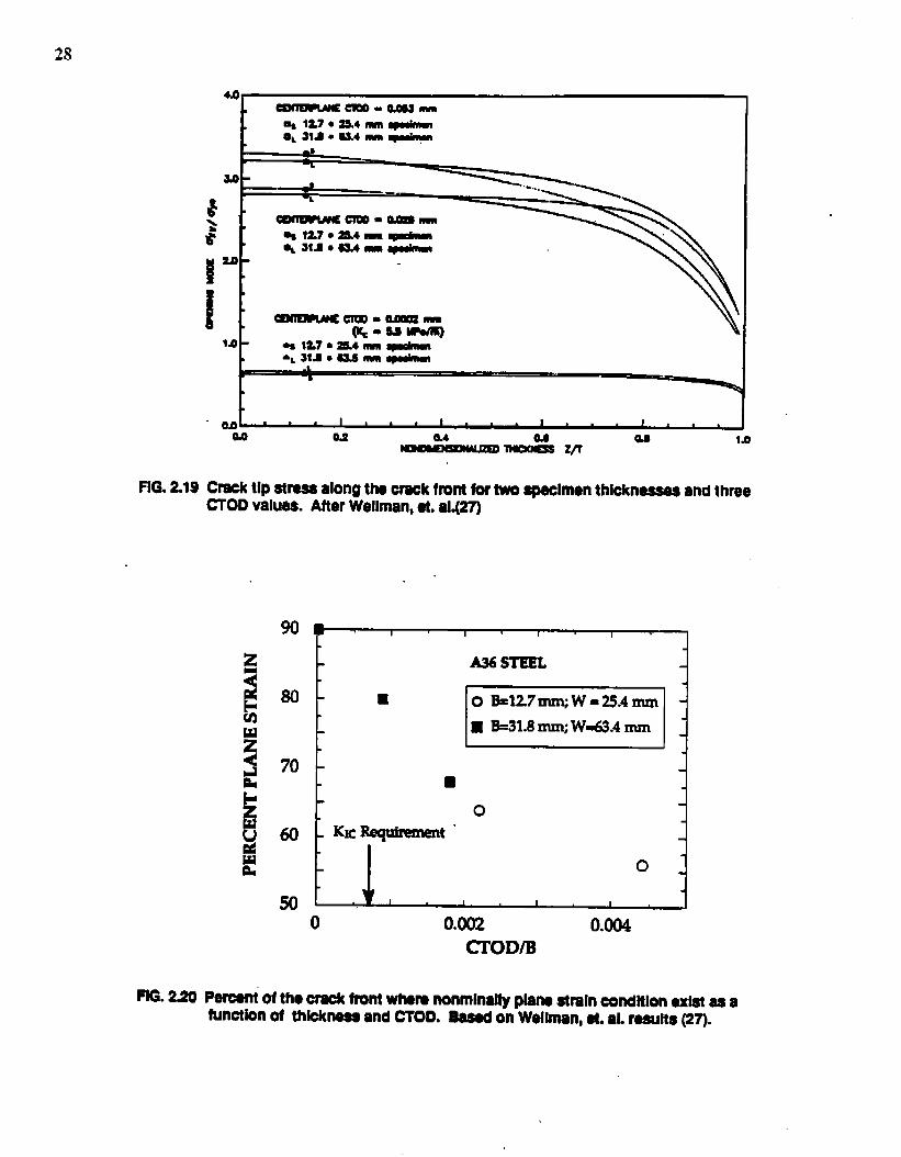
WeUman et al. (27) demonstrated the effect of thickness with three-dimensionalfm.ite element analysis of a fracture mechanics sped.men of A36 steeL I@re 219 is aplot of ~ along the mack front for two thicknesses and three ~D values,corrqmuii.ng to 9 = Oand a constant r value near the crack tip. The normalizedthickness refers to the relative psition along the mack front Z/T= Ocorresponds to

26

\ SMALLTEST SPECIMEN

\IARGE STRUCTURE ~

region

\

/

Lm qj

2.10

LoGr

Schematic atraaa flolds In ● mall teat Specimen and ● largeto the aamo applbd J.

27

the center ofthe specimen and Z/T= 1.0 corr~ponds to an outer edge. Note thatnear the center of the specimen the am- are flat, indicating plane strain conditions.Near the edge of the spedmen, strws decreases rapidly ss the plane stress limit isapproached. The S@ of iihe plane strain region decre~ with increasing CTOD.The thicker specimen has a larger relative plane strain region at a constant ~OD, aneffect is seen more clearly in Hg. 220, which is a plot of the relative size of the planestrain region versus ~D/thi~s. For this plot, the hmdary ~ tie plane strti.region was defined arbitrarily as the point where the str=s fell to 90 percent of thecmter plane value. me KICthickness requirement for this ma~rial is superimposedfor comparison According to Fig. 220, approximately 85 percent of the crack front isin plane strain when Eq. [~] is satisfid The thi~s requirement of Eq. [230] forthis material corr~nds to CTOD/B = O.= which is well off the scale of Fig. 220.Thus the crack front of a s@men that Just satisfi~ the JIc standard has less than 50percent plane strain along the Ua& tit. Whether or not this is -dent tomeasure a fracture toughness vslue indicative of pure plane strain conditionsdepends on the microme&anism of fracture.

2.4 MICROMECHANISMS OF FRACTURE IN FERRITIC STEEL

Fracture in steel parent material and ‘welds usually occurs by one of threemechanisms:

1.

z

3.

Transgranular cleavage

Miaovoid coales&nce

Intergramdar fracture

Cleavage is rapid, unstable fracture usually associated with brittle materials, whilemicrovoid coal-ence (or ductile tearing) can occur in a slow, stable manner.Intergranular macking can & either ductile or brittle. It is wnmlly astiated with acorrosive environment, grain boundary segregation, or both. In the absence ofadverse environmental renditions and detrimental heat treatments such as temperembrittlement, fracture in ferritic materials nearly always =curs by mechanisms (1)and (2). Consequently, this section _ on cleavage and microvoid coalescmce

Cleavage occurs when the kal stress is stiaatt to propagate a mack nucleus thatforms horn a microstructural feature such as a carbide or inclusion. For ductiletearin& a aitical strain must be reached for the coalescence of voids that formaround second phsse particl~. The fkacture toughness will necessarily differ for thedifferent fracture mechanisms (2$).

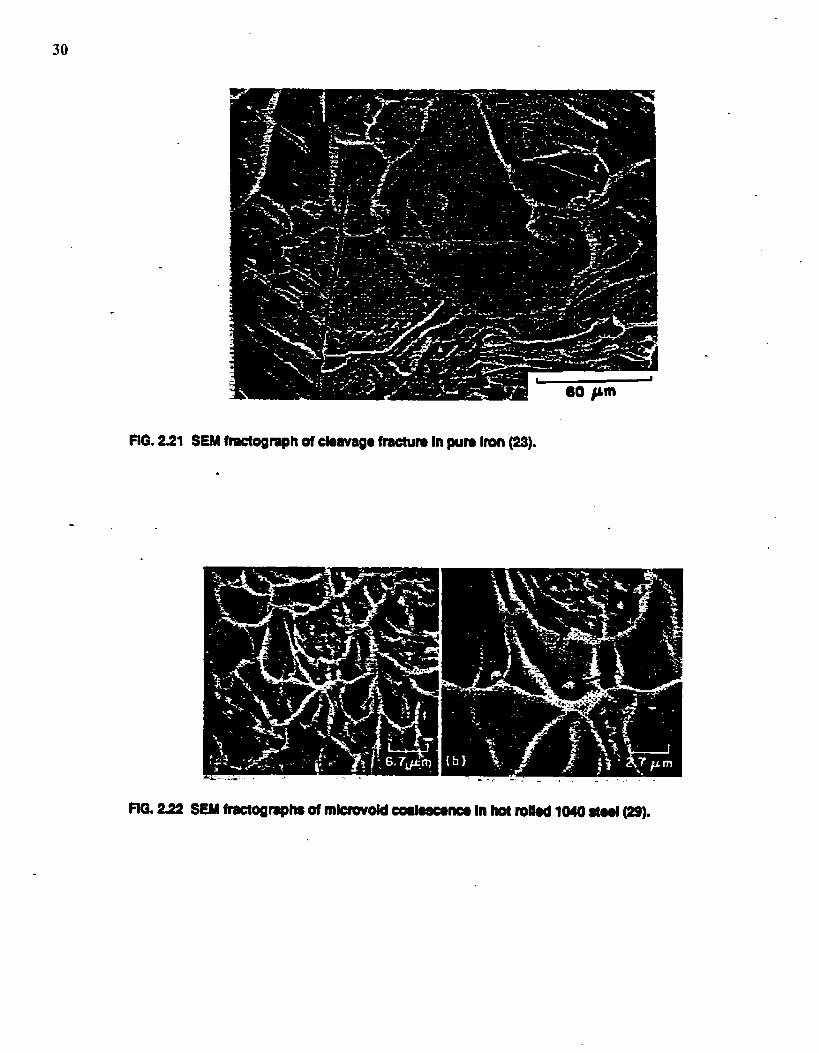
Hgur= 2.21 and 2.22 are scanning electron mi~oscope (SEM) fractographs thatcompare the appearance of the two fracture mechanhs (2349). Cleavage produc- arelatively flat, faceted surface because the fracture propaga- along spedfic

28

d I 1 I I

PIG.219 Cnacktlp atreaa alongthe crack front for two apeolmenthlckneaaeaand three~OD value% AfterWellman, et. aL(27)

PIG.220

80

70

60 L KICRqinmwnt ‘

M6 STEEL

=

o

0

so ‘. v I 1 1 1

0 0.002 0.004~OD/B

Pe~~ of the c-front when rtonmlnaltyplane$tMln CoMtlOn exist aa afunctionof thkknasa and CTOD. Baeedon Wellman,@t.aL reaulta (27).

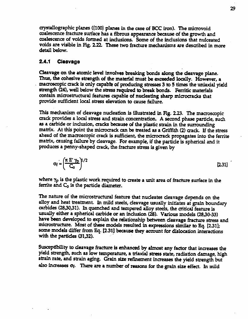
29

~two~aphic planes ((100] planes in the case of BCC iron). The microvoidcoalescence fracture surface has a fibrous appearance because of the growth andcoakcence of voids formed at inclusions. Some of the inclusions that nulceatedvoids are visible in Fig. 2.ZL Tke two fracture mechanisms are destikd in moredetail Mow.

2.4.1 Cleavage

Cleavage on the atomic level involves bre&ixig bonds along the cleavage plane.Ihus, the coh~ive strength of the material must be exceeded locally. However, a

- maaoscopic crack is only capablk of producing str~ 3 to 5 tire= the uniaxial yieldstrength (24), well below the str~s required to break lxmds. Ferritic materialscontain mimostructural featu.m capable of nucleating sharp microcracks thatprovide sfident local str~s elevation to cause failure.

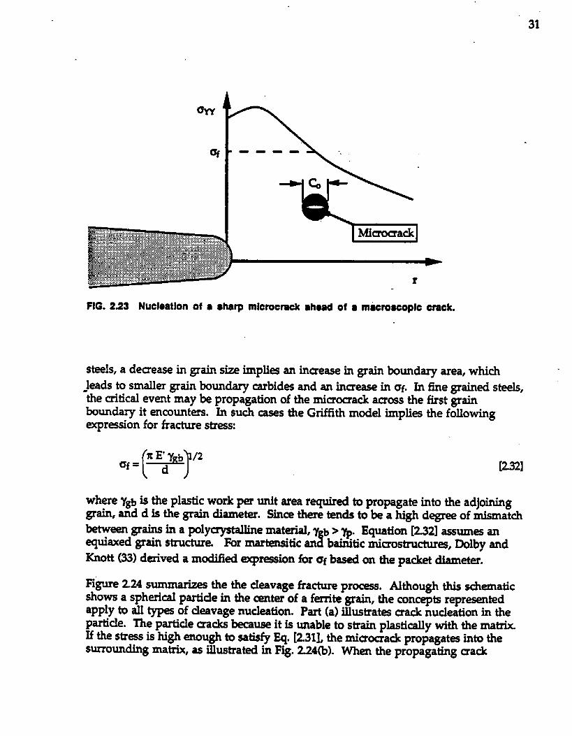
This mechanism of cleavage nucleation is illustrated in Fig. 223. The mamoscopicmack provid~ a local stress and strain concentration A second phase particle, suchas a carbide or inclusion, sacks because of the plastic strain in the surroundingmatrix. At this point the rnicrocrack can b treated as a Grifiith (2) sack If the stressahead of the mamoscopic mack is sficient, the microcrack propagates into the ferrite -ma&ix, causing failure by cleavage. For ~ample, if the particle is spherical and itprodue a penny-shaped uack, the fracture stress is given by

(1=f= zE’yp /2G

where Ypis the plastic work required to aeate a unit area of fracture surface in thefenite and q is the particle diameter.

The nature of the mimostructural feature that nucleates cleavage depends on thealloy and heat treatment. In mild steels, cleavage usually initiates at grain boundarycarbid= (28#lsl). In quenched and tempered alloy steels, the critical feature isusually either a spherical carbide or an inclusion (28). Various models (28s0-33)have been developed to explain the relationship between cleavage fracture str~s andmiaostructure Most of ~ mmkl.s renilted in exp=sions similar to Eq. [231];some models differ from Eq. [231] kxue they account for dislocation interactionswith the p-tick (31s2).

Susceptibility to cleavage fracture is enhanced by almost any factor that incre~ theyield strength, such as low temperature, a triaxials- state, radiation damage, highstrain rate, and strain aging. Grain sin rehement inuea,ss the yield strength butalso incr~ q. There area num&r of reasons for the grain size effect. In mild

30

FIG.221 SEM frmogmph of cleavagofracturoInpuraIron(23).

.

FIG.222 SEMfracmgmphsd mkfovoldcuml-- Inhatrol~ 10408tool(29).

31

FIG. 2.23 Nucleation of ● sharp mlcroerack ●head of ● mjcroaooplc crack.

steeIs, a decrease in grain size implies an increase in grain boundary area, which-leads to smaller grain boundary -bides and an increase in of. In fme grained steels,the critical event may be propagation of the rnicr~ack amoss the first grainboundary it encounters. In such cases the Grifiith model implies the following~r=sion for fracture str~s

where 7,b is the plastic work per unit area required to propagate into the adjoininggrain, and d is the grain diameter. Sine there tends to be a high degree of mismatch&tween grains in a pdyuystalline material, y b > ~. Equation [232] assum~ an

iequiaxed grain structure. For martensitic an ba.initic microstructure, Dolby andKnott (33) derived a md.i.iki expr~ion for ~f based m the packet diameter.

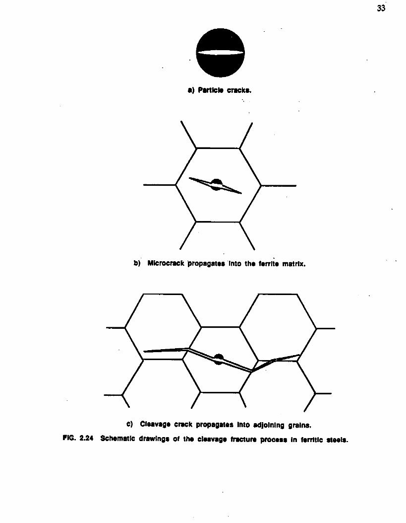
Rgure 224 swmwizes the the cleavage fracture process. Although this sdwrnaticshows a spherical particle in the anter of a ferrite grain, the concepts representedapply to all types of cleavage nucleation. Part (a) illustrates crack nucleation in theparticle. The particle sacks &cause it is unable to strain plastically with the matrixIf the stra is high enough to satisfy Eq. [231], the micromack propagat~ into thesurrounding matrix, as illustrated in Fig. 224(b). When the propagating sack

32

rea- the grain boundary, it must change orientation to align itself with the near~tdeavage plane of the next grain (Fig. 224c), requhing additional work, as discussedabove.

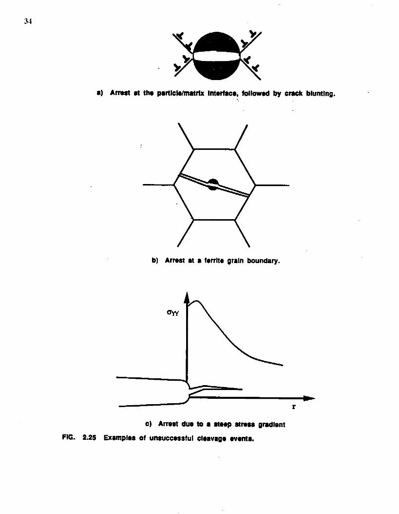
In some m cIeavage nucleat-, but total fracture of the s@rnen or stnacture willnot occur. Hgure 225 illustrat= three examples of unsucc=sful cleavage events.Part (a) shows a miaouad that has arrested at me particle/mati interface. The -pariide crack due to strain in the matrix, but the crack is unable ~ propagate kausethe applied stms is less than the required fracture stra. This miuocrack d- notrc+i.nitiate bcause subsequent deformation and dislocation motion in the matrixcam the uack to blunt Mi-adcs must remain sharp in order for the str~ onthe atomic level to ex~ the mhesive strength of the material. If a mimmack in aPar&le propaga- into the femite matrix, it may amst at the grain Im.ndary, asillustrated in Fig. 225(b). This com~ponds to a case where Eq. [232] governscleavage. Even if a mack successfully propagates into the ~ounding grains, it maystill armt if there is a steep stress gradient ahead of the mamoscopic crack (Fig. 225c).This tends to occur at low applied KI valu~. Lcdly, the strss is stiaent to satisfyEqs. [231] and [2.32] but the str=s decays rapidly away fmm the macroscopic sack andeventually can no longer satisfy the Griflith energy uiterion.

The phenomena illustrated in Fig. 225 have been observed ~rimatally.Gerberich (34) monitored fracture toughnes tests with acoustic emission andobsemed many micrdeavage events before ilnal fracture. Lin et sl. (35) providedmetallographic evidence of cracked carbides and mack arrest at grain boundaries in a1008 spherodized steel. Imin (36) obsemed numerous cleavage initiation sites onthe fracture surfaces of notched round bars which were tinted at very high strainra~. The dynamic loading caused cleavage nucleation at very low KI values. Theseearly cleavage events arr~ted, apparently because of the steep str~s gradient. Finalfailure of each specimen occurred when the applied K1 was sufiiaent for a crack topropagate through the spedmen.

Cleavage fracture is a weakest link phenomenon. A spedmen or structure needsonly one uitical mimostnactural feature for mtastrophic failure to occur. The localfracture str~s depends on the largest or most favorably oriented particle that occursin the material near the tip of a macroscopic crack A i%ite amount of materialmust be sampled in order to ilnd a dical pa-tide. R&Meet al. (37) were among thefit to recognbe this when they propsed a simple model for cleavage. Their modeIstat= that cleavage will occur when the uitical fracture str~s, af, is exceeded over acritical distanm, ~ ahead of the aadc tip. They assumed that af and ~ were single -valued material constants. Curry and Wott (38) used a statistical argument todevelop a model in which a uitical sample voh.une was required in order to causefailure. Later, Curry (39) demonstrated that their statistical interpretation of cleavagewas essentially equivalent to the Ritchie et al. model. Recently, a number of moresophisticated statistical models for cleavage fracture have been developed(35,4044).Th- models predict the effect of microstructure on fracture toughness. In additio~

33”

- e● Pw’tlcla cracks.

b) Mlcrocmck propagates “Into tho fmfic matrix.

c) Cl$8Vag0 crock propagates Into adjolnlng grains.

FIG. 2.24 Schemstlc drawings of ths elaavago fracturs procass In forrttlc stssla.

34

●) Arrast at ths patiIcls/matrtx Intorfaeo, followsd by emok blunting.-.

b) Arrast at a forrlto grain boundary.

H

C) Arrest due

FIG. 2.25 Examples of unwcccssful

to s StOepstraas

cloavago avonts.

r

gradlsnt

35

the statistical models quantify the scatter in fracture toughness data, which is a directrwlt of the weakest link nature of cleavage. ‘Ibis scatter is particularly severe in theductil-brittle transition of steels. Some of the methods for anal@ng Scatt= aredesuibed in Section 3.5.

2.4.2 Microvoid Coalescence

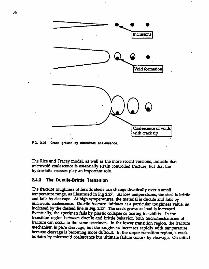
h ferritic steals, as the temperature inmeases and”.theflow stress d=eas~ it becomesmore difficult to produce high enough str~~ to initiate cleavage. When conditionsbr cleavage are unfavorable a ductile fracture mechankn, rn.bovoid coalescence,oprate. This is the dominant fracture mechanism of FCC alloys, even at very lowtemperatures. The typical m.icrostructural chan~ which occur during initiationand growth of a fibrous sack are (28}

L Formation of a free surface at a second phase particle or inclusion by eitherinterface decohesion or particle cracking

2 Growth of a void around the particle, with the aid of hydrostatic stress

3. Coalescence of the growing void with the sack tip

Qack growth by microvoid coakscence is illustrated schematically in Rg. 226. Theabove events occur continuously as the mack advanc~. That is, as voids at the cracktip coalescence, additional voids nucleate and grow further away from the sack tip.A numk of models have been developed to describe this fra@ure process (4~7).Rice and Tracey (45) proposed the following equation to d~cribe the growth of avoid.

[233]

where R is the void radius, ~ is the initial radius, ~ is the equ@lent plastic straintand ~m is the mean (or hydrostatic) stress, defined as

B]

Rice and Tracey assumed a nonhardening material in their analysis. More recentmtiels (46,47) have moclifmd the above =pression to take account of strainhardening.

36

QQ*

Coalescenceof voids Iwith crack tip I.. .-

Fl@ 226 Crack growthby microvold omloscona.

The Rice and Tracey model, as well as the more recent versions, indicate thatrrkovoid coalescence is essentially strain controlled fracture, but that thehydrostatic stresses play an inqmrtant role.

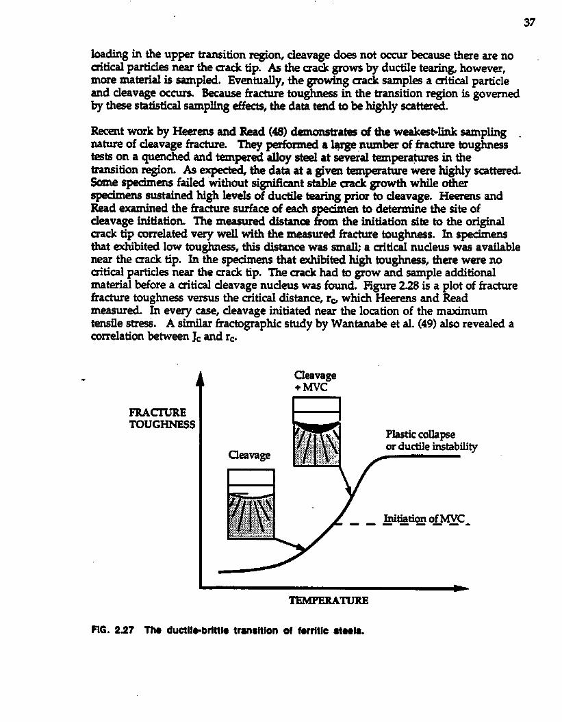
2.4.3 The DuctlleBrittle Transition

The fracture toughn=s of ferritic steels csn change drastically over a smalltemperature range, as illustrated in FIg 227. At low temperatures, the steel is brittlesnd fails by cleavage. At high tem~atum, the mataial is ductile and fails byrnicrovoid coalescent. Ductile fracture initiate at a particular toughness value, asindicated by the dashed line in Hg. 227. The sack grows as load is increased.Eventually, the specimen fails by plastic collapse or tearing instability. In thetransition region between ductile and brittle behavior, both micromechanisms offracture can mmr in the same spednen. Jn the lower bansition region, the fracturemechanism is pure cleavage, but the toughn~s incre~ rapidly with temperaturebecause cleavage is becoming more difihdt. In the upper transition region, a crackinitiates by microvoid coalescence but ultimate failure occurs by cleavage. On initial

.

..37

loading in the upper transition region, cleavage does not occur because there are nouitical particles near the crack tip. A the ~ack grows by ductile teari.n~ however,more material is sampled. Eventually, the growing crack sampl- a critical particleand cleavage occurs. Because fracture toughness in the transition region is governedby tbe statistical sampling effects, the data tend to be highly scattered.

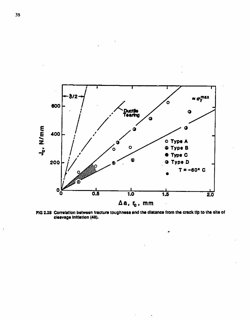
Recent work by Heerens and Read (48) demonstra- of the weakt-link sampling .nature of cleavage fracture. They @ormed a large number of fracture toughness-ts on a quenched and tempred alloy steel at several tem~atures in thetransition regiom As_ the data at a givm temperature were highly sattered5ome spedmens failed without signibnt stable sack growth while otherp- sustained high levels of ductile tearing prim to cleavage. Heerms andRead examined the fracture surface of each spedmen to detemme- the site ofcleavage initiation The measured distance from the initiation site to the originalsack tip mrrelated very well with the measured fracture toughn~s. Jn spedrnensthat exhibited low toughn-, this distance was small; a critical nucleus was availablenear the mack tip. In the specimens that exhibited high tougluws, there were nocritical partick near the crack tip. The sack had to grow and sample additionalmaterial &fore a aitical cleavage nucleus was found. Figure 2.28 is a plot of fracturefracture toughness versus the dical distance, re which Heerens and Readmeasured. In every case, cleavage initiated near the location of the msximumtensile str~. A similar fractographic study by Wantanabe et al. (49) also revealed acorrelation IWw=n Jc and rc.

Cklvage+ Mvc

I I

Plastic collapse

a=~~or ductile instability

Initiation of WC---- ----

TEMPEUTURE

FIG. 2S7 Tha duotll~brtttl~ trans~lon of f.rfitlc St-1a.

38

EE2

400

200

0,

FIG238

u.= 1.U la z

Aa, ~, mmCor?elatlonbetweenfracturetoughness●d t!wdlstancs from the crack tlp to the she ofclsavagoInttlatlon(48).

.

39

3. FRACTURE TOUGHNESS TESTING

A fracture toughnesstest meamm tie resistanceof a material to crack extensio~ -Such a t~t may yield either a single value of fra&re toughness or a r~tance cume,where a toughness parameter SUA as K, J, or -D is plotted a@inst sack extension.A single toughn~ vslue is usually suffi&nt to dtih a @t that fails by cleavage,kause this fracture mdanism is typically unstable. The situation is similar to theschematic in Fig 22(a), which illustrat~ a material with a flat R eumm For reasonsdiscussed in Section 3.6, cleavage actually has a falling R tune after initiation Crackgrowth by mimovoid coslesence, however, usually yields a rising R -e, such asthat shown in Fig. 22(b). Thus ductile mack growth can be stable, at least initially.When ductile crack growth initiates in a test specimen, that specimen seldom fsilsimmediately. Therefore one can quantify upper shelf fracture toughness either bythe initiation value or by the entire r~istance cu.nm

There are several ASTM standards for fracture toughness testing. The KIc standard,ASTM E399-83 (25), is intended for relatively brittle materials or thick sections. TheJIC s~dard, ~~ E813-87 (261, measur= a J value near initiation of ductile tearing.Another stsndard, E1152-87 (50), giv~ guidelines for measuring a J resistance cume.A CIOD testing standard has been published recently ASTM E1290-89 (51).

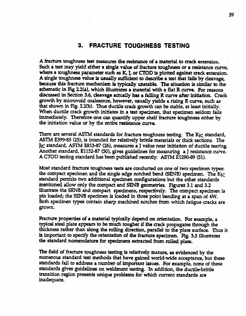
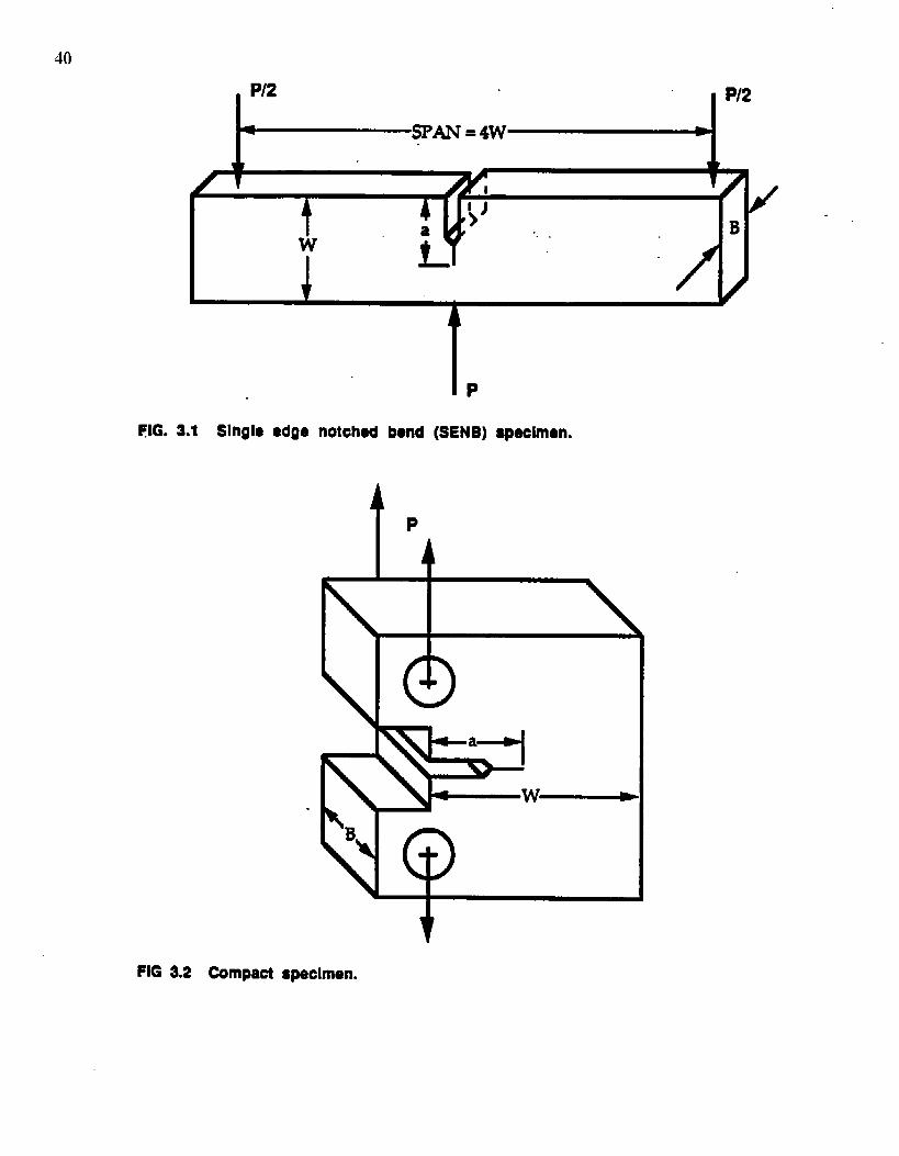
Most standard fracture toughness tats are conducted on one of two specimen types:the compact specimen and the single edge notched bend (SENB) spedmen. The K1cstandard permits two additional spedmen mfigu.rations but the other standardsmentioned allow only the mmpact and SENB geometries. Figures 3.1 and 3.2illustrate the SENB and compact spedmens, respectively. The compact specimen ispin loaded; the SENB specimen is loaded in three point bending at a span of 4W.Both spetien types contain sharp machined notches from which fatigue cracks aregrow. .

Fracture properties of a material typically d~nd on orientation For example, atypical steel plate appars to lx much tougher if the crack propagates through thethickness rather than along the rolling direction, parsllel to the plate surface. Thus itis important to spedfy the orientation of the fracture specimen. Fig. 33 illustratesthe standard nomenclature for s@nwns -acted from rolled plate.

The field of fracture toughnss ~ting is relatively mature, as evidenced by thenumerous stsndard t-t methods that have gained world-wide acceptance, but thesestandards fail to address a number of importsnt issues. For ~ple, none of thesestandards gives guidelin~ on weldment testing. In addition, the ductil~brittletransition region pr~ts unique problems for which current standards sreinadequate.

40

P/2 P/2

~ SPAN = 4W *

FIG. 3.1 Slnglo tdge notched

1P

bend (SENB)

t

P

4

spsclmen.

FIG 3.2 Compact specimen.

41

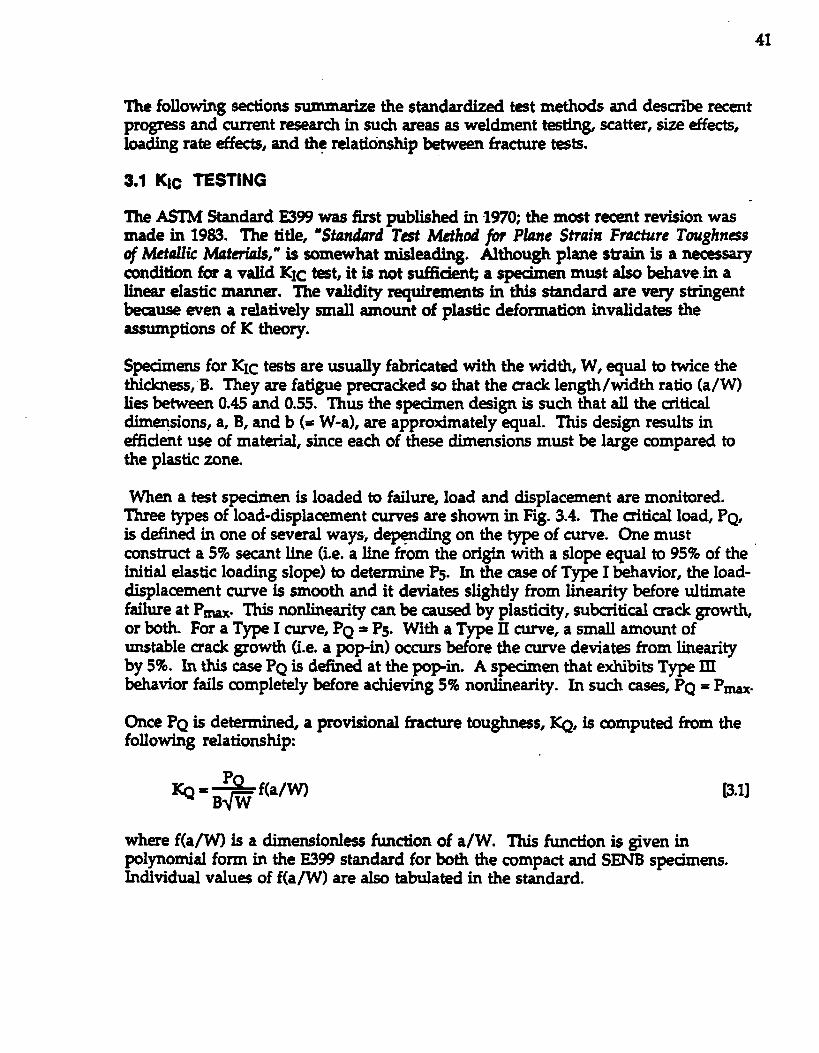
The following sections summarize the standardized t~t methods and desaibe recentprogress arid current research in such areas as wekhnent tdn~ scatter, size affects,loading rate effects, and the relationship &en fracture -ts.

3.1 KIc TESTING

The ASIM Standard E399 was first published in 19?o; the mat -t revision wasmade in 1903. The title, “StandurdTat Mdhd fbr Plane Sfraia Fracture Toughness#Metallic Zb4derids,” is somewhat misleading. Although plane strain is a necessarycondition for a valid KIc test,it is not suf&ient; a specimen must also khave.in alinear elastic manner. The validity requirements in this standard are very stringentbecause even a relatively small amount of plastic deformation invalidate theassumptions of K theory.

Specimens for KIC tests are usually fabricated with the width, W, equal to Mce thethickness, B. They are fatigue precracked so that the crack Iength/width ratio (a/W)Ii= between 0.45 and 0.55. Thus the specimen d~ign is such that all the aiticald.im~ions, a, B, and b (= W-a), are approximately equal. This design radts ineffiaent use of material, since each of these dimensions must be large compared tothe plastic zone.

When a t~t spedmen is loaded to failure, load and displacement are monitored.Three types of load-displacement -es are shown in Hg. 3.4. The criticsl load, PQ,is defuwd in one of several ways, depruling on the type of a.me. Une mustconstruct a 5% secant line (i.e. a line from the origin with a slope equal to 95% of theinitial elastic loading slope) to determm“ e P5. In the case of Type I &havior, the load-displacement tune is smmth and it deviates slightly from linearity before ultimatefailure at P- This nonlinearity can be causal by plastiaty, subcritical crack growth,or both. For a Type I cume, PQ = P5. With a Type II cume, a small amount ofunstable crack growth (i.e. a p@n) occurs before the cume deviat~ from linearityby 5%. In this case PQ is defined at the popin. A specimen that exhibits Type IIIbehavior fails completely before achieving S% nonlinearity. h such cases, PQ = P~~

Once PQ is determined, a provisional fracture toughness, ~, is mmputed from thefollowing relationship:

B*1]

where f(a/W) is a dimensionless function of a/W. This function is given inpolynomial form in the E399 standard for both the compact and SENB spedmens.Individual value of f(a/W) are also tabulated in the standard,

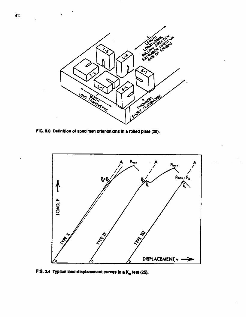
FIG.34 DefInltlon@fepeclmen orientetbne {n 8 rol~ plsta (23).

flG. ~4 TypkalWdlsplaoement curvesin● ~ W (35).

43

Recall from Section 2.2 that ~rasions for K can always be reduced to the form ofEq. [26]. Equation [3.1] is no exception- If we define a dtara~tic StieSS M P/(BW),the gmmetry comtion factor for the compact and SENB specimens is given by

r)Y= f(a/W) —1/2 “

rca[32]

The characteristic str~s, P/(BW), has no physical meaning for tlwe -t spinwn.s. since they are loaded predominantly in bending. Thus Eq. [3.1] is a more cornmientfmm in this case than.Eq. [21].

The ~ value computed from ~q. [3.1] is a valid KIc tit only if all validityrequirements in the standard are rne~ The main validity requimrmts are asfollows.

p-$ I.lo PQ [33b]

The Iast requirement is a restatement of Eq, [2.29]. If the test meets all of the abovecriteria as well as additional .requimments of ASTM E399, then KQ = KIC,

- Most sbwtural steebcannot meet the validity requirements of E399except at veryIow temperatures, as demonstrated by a few sample calculations. Consider amedium strength steel with ~s =50 ksi On the upper shelf, the fracture toughness

comqmnding to initiation of ductile crack growth is typimlly around 200 ksi &forsuch materials (23). Substituting th- values for strength and toughn~s into Eq.[3.3c], reveals that a fra-e tou@mss specimen must b 40 in thick to obtain a validKIC ! If the 50 ksi material is produced as 1 in thick plate, the maximum valid KIc

that can & measured is 32 ksi ~. If a structure made from a material with thistoughness were loaded to half the yield strength (25 ksi), the mitical mack size(estimated horn Eq. [Z5]) wdd b approximately 0.5in. If W were a weldedstructure with yield magnitude residual stres~, the critical ~ack size would only be0.06 h

Thus it is virtually inqmssible to perform a valid KIc test on most structural steels atambient temperatures. Such a material could meet the validity requirements with areasonable section thickness only by -r fabrication practice or by cooling thematerial so that it is on the lower shelf of toughn~s. In either case, the materialwould probably be too brittle for structural application. When linear elastic -t

44

methods are invalid, fracture toughness must be quantii5ed by an elastic-plasticparameter such as J or ~D.

3.2 JIc AND J-R CURVE TESTING

There are two ASTM standards currently for J sting. The JIC st~dmd, lU13(26),which was &st published in 1981 and revised in 1987, outlines a -t method forsstirnating the uitical J near initiation of ductile Uack growth. me J-R cume testing -standard, El152(50), WaSht published in 19S7. ‘

Roth =t methd.s produce a J-R tune, a plot of J versus sack extensiom The E1152standard applk to the entire J-R ~~ E813 is ~ncerned only with JIG a single@ntontheRcuna Thesame~tcan &rqmrtedin terms ofkthstandards. This

- is analogous to a tensile -t, where one can report either the yield strength or theentire stms-strain curve.

In the case of the JIC standard, the R cume can be generated by either multiplespcimen or single specimen techniques. With the multiple specimen technique, aseries of nominally identical specimens are loaded to various levels and thenunloaded. Some stable sack growth occurs in most spedmens. This crack growth ismarked by heat tinting or fatigue cracking after the test Each specimen is thenbroken open and the sack ~tension is measured. The most common singlespecimen test technique is the unloading compliance method. The mack length iscomputed at regular intemaJs during the test by partially unloading the specimenand measuring the compliance. As the mack grows, the specimen becomes morecompliant (less stiff). Both E813 and E1152 provide polynomial expressions thatrelate a/W to compliance. An alternative single specimen test method is thepotential drop procedure, yet to be standardized by ASINi, in which sack growth ismonitored through the change in electrical r~istance which accompanies a loss inaoss sectional area. Both single spedmen procedures are practical only inconjunction with a computer data acquisition and analysis system.

Regardless of the method for monitoring crack growth, a Conesponding J value mustbe computed for each point on the R cume. For estimation purposes, both standardsdivide J into elastic and plastic components

The

J= JeI + JpI [3.4]

elastic J is computed from the elastic stress intensity

m-v)h=~ [351

where K is computed horn load with Eq. [3.1]. The JIC standard enable the plastic J ateach point on the R cume to be estimated from the plastic area under the load-displacement me

45

M

where q is a dimensionless constant, API is the plastic area under the load-displacement -e (= Hg. 33), and b. is the initial lig~ent length For an SENBspecimen,

q=zo

For a compact specim~

n“2+0522bo/W

Equation [3.6] was derived

-.

J.3.7a]

mb]

from the energy release rate definition of J (Eq. [2-21]).

The J-R me testing standard requires a somewhat more detailed calculation of Jpl,performed incrementally since the sack length inmeases and the net cross-sectionalarea d-eases throughout the test. Since E81S87 is concerned with the initiationpoint rather than the shape of the R tune, the more detailed formula that comets Jfor crack growth is optional in JIC tests. In the limit of a stationary mack, bothformulas give identical results. Thus the measured initiation toughness isinsensitive to the choice of J equation.

The E813-87 procedure for computing JQ, a provisional JIG from the R cume isillustrated in Fig. 3.6. Exclusion line are drawn at crack extension (As) values of 0.15and 1.5 mm. These lines have a slope of 2GY, which corresponds approximately tothe component of =ack extension that is due to crack blunting as opposed to ductiletearing. A horizontal exclusion line is defined at a maxim&” valu~-of ~

All data that falI within the exclusion limits are fit to a power law expression

J= C1(MQ

The JQ is defied as ihe intersecdon between Eq. [3.9] and a 0.2 mm offset line.other validity aiteria are met, JQ = JIC as long the following size requirementssatisfied

[3$1

[3.9]

Ifallare

[3.10]J

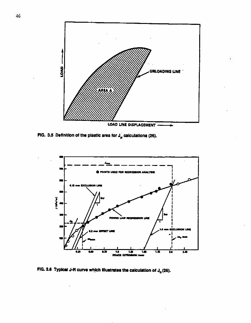
LOAD UNE DISPLACEMENT~

FIG. aS Deflnltbn of the plastlcareaforJmcakulatbna(26).

m

m

—— L——— ——— — ————. ~

gmluiauuomne~ AUUW48 I

~ ~ 1-}

FIG.~6 Typlal J-R CUWQwh.kh lllu8&rataatha cakubtlon of J* (26).

The J-R cume standard has limits on J- and crack extension relative to spedmen*.

2oJm .B,~2—

%’[3.H1

and-.

Aam s 0.10 b. p.u]

F@re 3.6 (50) shows a typical J-R cume with the E1152-87 validity Iimi@. The.~~on ~ ~ J-R me Mat f~ outside W limits is considered invalid. Note‘tkil the hut a J- in ASTM E1152-87 is more severe than the J-x limit of ASTME813-87 (Eq. 3.8]), but this limit is 1ss restrictive than the JIC size aiterion @q. [3.10]).

3.3 CTOD TESTING

Because of the strict limits on plastic deformation, the KIC =t can only be used onthe lower shelf of toughness in structural steels and welds. The JIC and J-R muve testmethods allow considerably more plastic deformation, but these tests are only validon the upper shelf. The ~OD testis currently the only standardized method tomeasure fracture toughness in the ductikbrittle transition region.

- The fist CTOD t=t standard was published in Great Britain in 1979(52). ASTMrecently published E1290-89, an Am~can version of the CTOD standard. The BritishCTOD standard allows only the SENB specimen; the ASTM standard provides forCTOD measurements on both the compact and SENB specimens. Both standardsallow two configurations of SENB specimens: 1) a rectangular ~oss section with W =2B, the standard geometry for KIC and JIC tats; and 2) a square uoss section with W =B. The rectangular specimen is most useful with L-T or T-L orientations (see Fig.33); the square section is generally used in the L-S or T-S orientations.

Experimental CTOD Wmata are made by separating the CTOD into elastic andplastic components, similar to the JIC and J-R ~~. The elastic ~OD is obtained‘komthe elistk~

The ehstic K is related to applied load through Eq. [21].assure= that dn = 0.5 for linear elastic conditions (see Ea

[3.13]

The above relationship[2261). The DktiC

mmponent of ~OD is obtained by assuming that the t~~ s~en r~tats about aplastic hinge. This concept is illustrated in Fig. 3.7 for an SENB spedmen. The

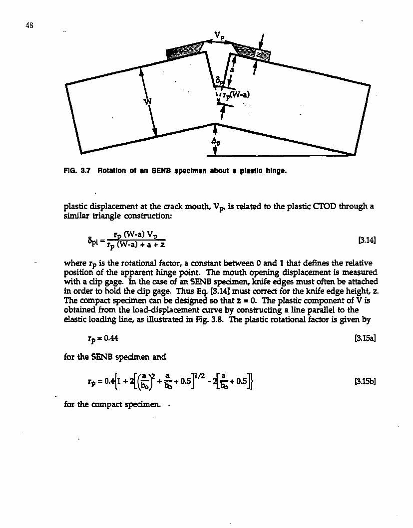
4s

FIG. 3.7 Rotationof an SENB speclmtn ●bout a plaatlc hinge.

pIastic displacement at the craEk mouth, Vp, is related to the plastic CTOD through asimilar triangle construction

r (W-a) VPbl=rP~W-a)+a+2

where rp is the rotational factor, a constant between Oand 1 that defines the relativeposition of the apparent hinge point. The mouth opening displacement is measuredwith a clip gage. h the case of an SENB sped.men, knife edge must often be attdwdin order to hold the clip gage. Thus Eq. [3.14] must comet for the knife edge height, z.The compact specimen can be d~igned so that z = O. The plastic component of V isobtained from the load-displacement muve by constructing a line parallel to theelastic loading line, as illustrated in Fig. 3.8. The plastic rotational factor is given by

rp = 0.44 [3.15a]

for the SENB specimen and

rp=4+w+&+”*’11’2-{5+’4for the compact spedmen. -

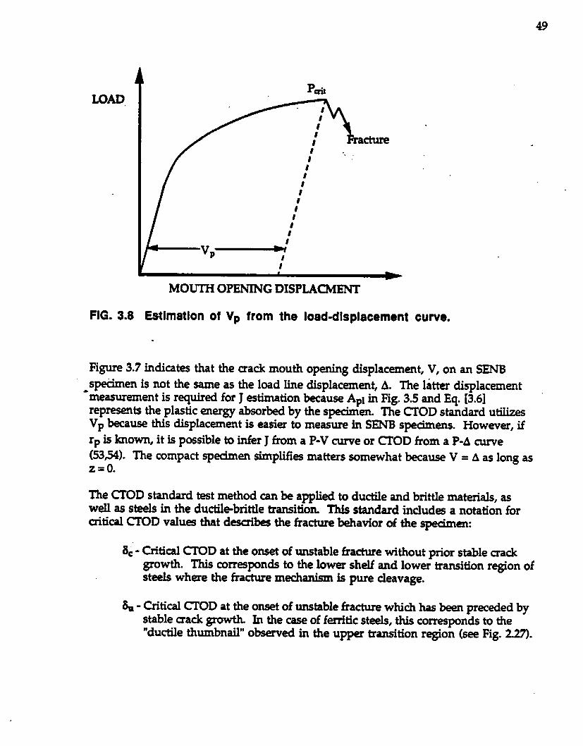
LOADP*

1

MOUTH OPENING DISPMCMENT

FIG. 3.8 Estimation of Vp from the ioad-displacement curve.

Figure 3.7 indicates that the crack mouth opening displacement, V, on an SENBspe6rnen is not the same as the load line displacement, A. The latter displacement

‘measurement is required for J estimation lwcause API in Fig. 3.5 ~d Eq. [3.6]represents the plastic energy absorbed by the specimen. The CTOD standard utilizesVP because this displacement is easier to measure in SENB specimens. However, if

rp is known, it is possible to infer J from a P-V curve or CI’OD from a P-A cume(53S). me compact spedmen simpliks matters somewhat because V = A as long asZ=o.

The CTOD standard test method can be applied to ductile and brittle materials, aswell as steels in the ductilebrittle transition This standard includ~ a notation forcritical ~D valu= that d-h the fracture behavior of the specimem

6C- Critical CT’OD at the onset of unstable fracture without prior stable crackgrowth. This correspds to the lower shelf and lower transition region ofsteels where the fkacture mechanism is pure cleavage.

~ - Critical CTOD at the onset of unstable fracture which has been preceded bystable mack growth. In the case of ferritic steels, this corresponds to the“ductile thumbnail” observed in the upper transition region (see Fig. 227).

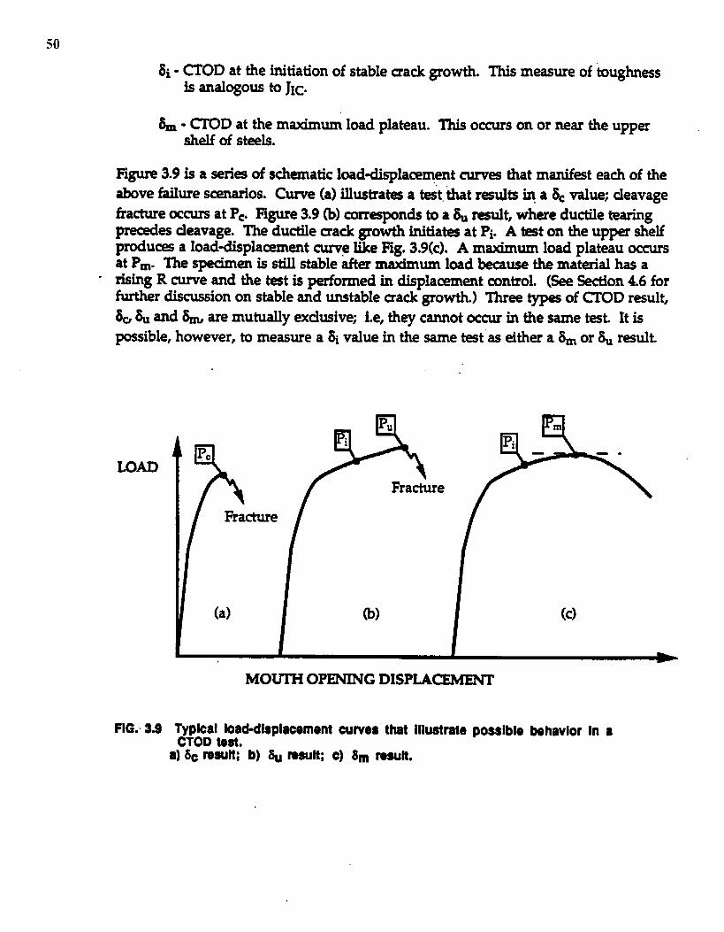
50

Si - CTOD at the initiation of stable sack growth. This measure of toughnessk ad~o~ b JIC.

~ - ~OD at the maximum load plateau. ‘l’his occurs on or near the uppershelf of steels.

I@re 3.9 is a series of schematic Ioaddisplamment cun~ that manif~t each of thealmve failure scenarios. Cume (a) illustrat~ a -t that resadts iq a ~ value; cleavagefracture mws at Pe Figure 3.9 (b) correqmnds to a ~ result, wh~e ductile tearingprecedes cleavage. The ductile crack growth initia~ at Pi. A 1st on the upper shelfproduces a Ioadd.isplacernent cu.me like Hg. 3.9(c). A maximum load plateau occursat Pm. The spedrnen is still stable ~er maximum load bcause the material has a

- rising R curve and the t-t is performed in displacement control. (See -on 4.6 forfurther discussion on stable and unstable crack growth) Three types of CTOD result,

k% ad b me muwfly u~uive; i.e, they cannot ocmrr in the same tmt It ispossible, however, to measure a ~ value in the same t~t as either a ~ or ~ resuk

LOAD

FIG. 33

Lb-- (C)

MOUITi OPENING DISPIACEMENr

Typical Ioad=dlsplacement cuwes thet Illuetrete poeaIble behavior In aCTODteat.

a) &cl’8sult;b) ~ ~SUlt; C) 6M ~Wh.

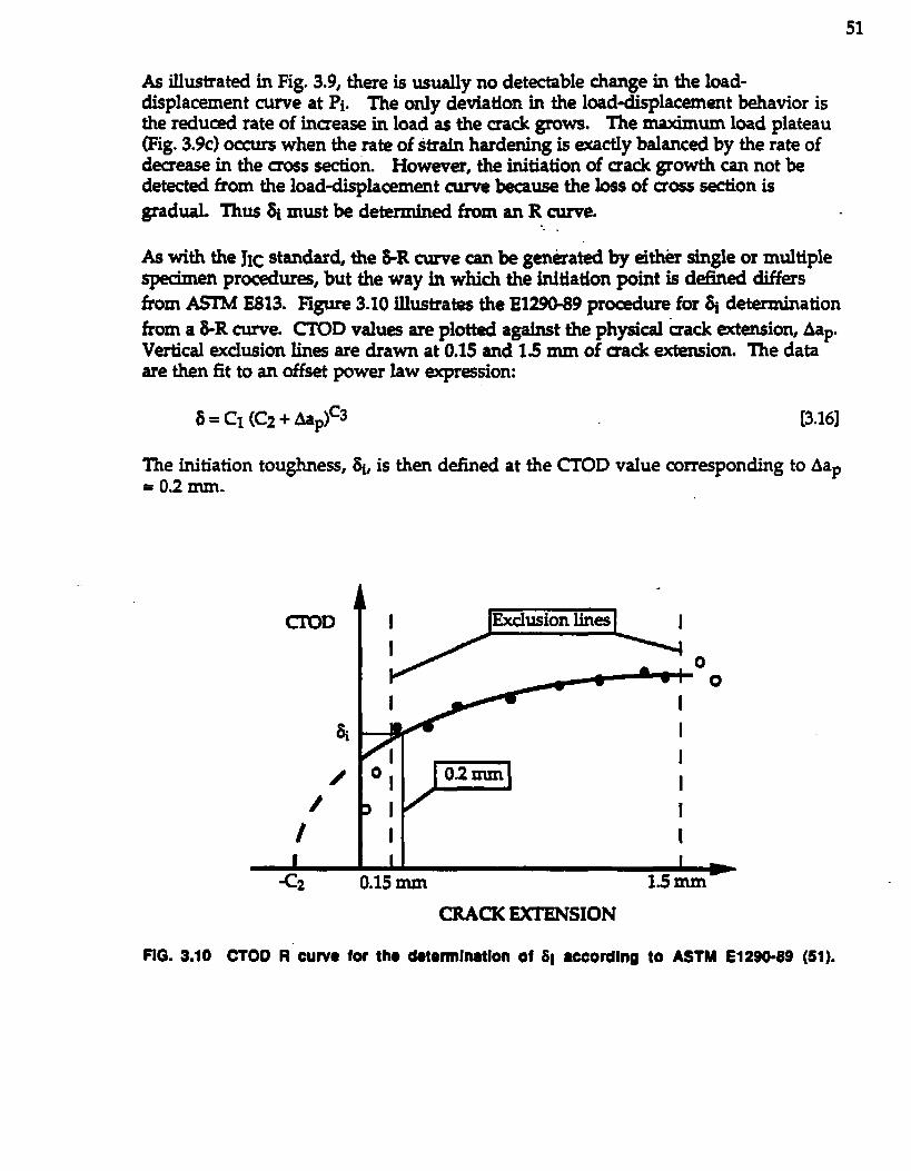
51

As illustrated in Fig. 3.9, there is usually no detectable change in the load-displacement tune at Pi. The only deviation in the load-displacement behavior isthe reduced rate of increase in load as the mack grows. The maximum load plateau(Fig. 3.9c) occurs when the rate of strain hardening is exactly balanced by the rate ofdmease in the aoss section. However, the initiation of crack growth can not bedetected from the load-displacement cmwe because the loss of cross section isgraduaL Thus ~ must be determined from an R cu.me.

As with the JIC standard, the&R cume can be generated by tithkr single or multiple_ pr-~e, but the way in which the initiation point is defined diffffsfrom ASIM E813. Rgure 3.10 illustrates the E1290-89 procedure for ~ determm● ation

from a&R cuwe. CICID values are plotted against the physical mack @ension, AapVertical exclusion lin~ are drawn at 0.15 and 1.5 mm of sack extension. The dataare then fit to an offset pwer law expression:

a = c1 (C2 + A@

The initiation toughness, ~ is then defined at the CTOD value comesponding= 0.2 mm.

CIOD ‘Yn

I

I

‘13 1 I

I

wo

[3.16]

to AaP

FIG. 3.10 CTOD R cuw@for th8 Uotonnlnatlon Of 51 acoordlngto ASTME1280-69 (51).

The only specimen size requirement of the British and ASTM CTOD standards is arecommendation to test full section thickn=ses. For example, if a stmcture is to bemade of 1 in thick plate, then B in the tst specimens should be nominally 1 in Ifthe spedmen is notched from the surface (’L-S or T-S orientations), a square sectionspecimen is required for B to equal the plate thiclm=s. The British ~OD standardallows a/W ratios ranging from 0.15 to 0.75, while the ASTM standard r~tricts the-Sible atw Valu= @ ~ r~ge of 0“= to ~“=” ~ ~ -M= **I ~ -TM .standard allowed a much wider range of aw in the square section specimen, butconcerns almut the possible variation of rP with a/W led the memkers of the ~CTOD task group to r=tict the allowable range until the uncertainties k rp ~~d hmolved- Future revisions of this standard will probably relax the a/W restriction.Shallow macked spedmms have certain advantages, particularly for weldment tests

(see Section 3.4).

The ASTM CTOD standard recogrdz~ that since it does not contain sizerequirements relative to the degree of plastiaty, the measured aitical ~OD valuemay be gmmetry dependent. The standard correctly assumes that if a test spedmen’sthickness matches that of the structure being evaluated, the mack tip conditions inthe specimen will beat least as severe as in the structure. Experimental data andnumericsl analysis indicate that a small scale bend specimen is more highlyconstrained than a large panel loaded in tension.

3.4 WELDMENT TESTING

All the standards discussed are suitable for spedmens extracted from uniformsections of homogeneous material, but welded joints have decidedly heterogeneous

tiaostructures and, in many cases, irregular shape. Weldments also containcomplex residual stress distributions. Existing fracture toughness testing standardsdo not address the spe&il problems assoaated with weldment testing. The factorsthat make weldment testing difficult (i.e. heterogeneous rnicrostructur~, irregularshap-, and residual stresses) also tend to increase the risk of brittle fracture inwelded structures. Thus, one cannot simply evaluate the regions of a structurewhere ASTM testing standards apply and ignore the fracture properties ofWeldments.

Although there are currently no fracture toughness testing standards for weldments,a numbr of laboratory and industri~ have signii3cant of experience in this area.The Welding Institute in Cambridge, England which probably has the most expertk,has recently published detailed recommendations for weldment t~ting (55). TheInternational Institute of WeIding (IIW) has produced a similar document (56),although not as detailed. The American Petroleum Institute (API) has publishedguideline for heat affected zone (HAZ) testing as part of a weld procedurecpah.fxation approach (57). Committees within ASTM and the British StandardsInstitute (BSI) are curently drafting weldment test methods, relying heavily on 20years of practical experience as well as the aforementioned documents.

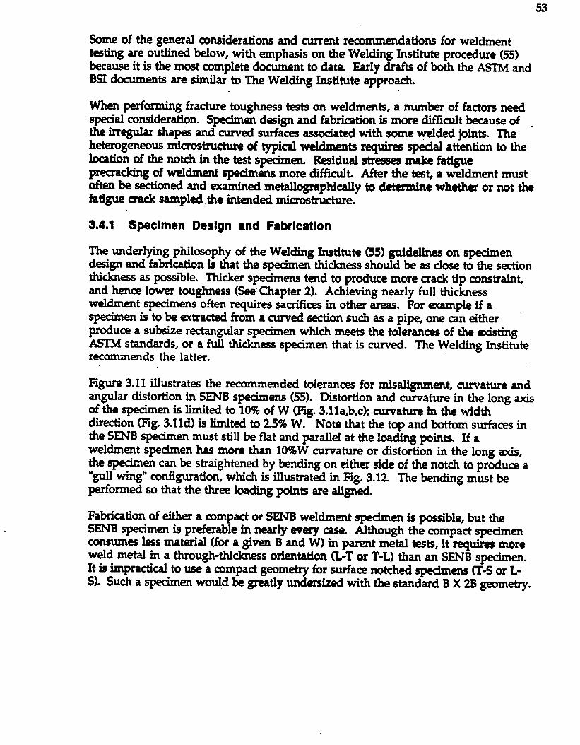
53

Some of the general considerations and cument recommendations for weldment~tig are outlined below, with anphasis on the Welding Institute procedure (55)&cause it is the most complete document to date. Early drsfts of both the ASTM andBSI dmmwnts are similar to The Welding Institute approach.

When perfoming fracture toughness ets on weldments, a num&r of factors needspecial consideration. Specimen d~ign and fabrication is more difficult -use of .the irregular shap and tuned surfa~ associated with some welded joints. Theheterogeneous microstructure of typical weldments requir~ spedal attention to thelocation of the notch in the test spdrnem Residual str~ make ktiguepmcracking of weldrnent -ens more cWmdt. After the test, a weldment mustOk be sectioned and examined metallographically to determine whether or not thefatigue crack sampled the intended microstructure.

3.4.1 Specimen Design and Fabrication

The underlying philosophy of the Welding Institute (55) guidelines on specimendesign and fabrication is that the spednen thickness should be as close to the sectionthickn=s ss possible. Thicker spedmens tend to produce more mack tip constraint,and hence lower toughness (See”Chapter 2). Achieving nearly full thicknesswekhnent specimens often requires ~miiic~ in other areas. For example if aspecimen is to be =tracted from a cunwd section such as a pipe, one a either -produce a subsize r-angular spedmen which meets the tolerancw of the existingASTM standards, or a full thickness specimen that is cu.wed. The Welding Instituterecommends the latter.

Figure 3.11 illustrates the recommended tolerances for misalignment, -ature andangular distortion in SENB spe&wns (55). Distortion snd cumature in the long axisof the specimen is limited to 10% of W (Fig. 3.lla,b,c); cumature in the widthdirection (13g. 3.lld) is limited to 25% W. Note that the top and bottom surfaces inthe SENB spedmen must still be flat and parallel at the loading points. If aweldment specimen has more than 10%W cumature or distortion in the long axis,the specimen can be straightened by bending on either side of the notch to produce a‘gull wing” contigu.ration, which is illustrated in 13g. 3.12 The bending must beperformed so that the three loading points are aligned.

Fabrication of either a mmpact or SENB weldment spedmen is possible, but theSENB specimen is preferable in nearly every case Although the compact spedmenconsumes 1ss material (for a given B and W) in parent metal tests, it requires moreweld metal in a through-thickness orientation (L-T or T-L) than an SENB specimen.It is impractical to use a compact geometry for surface notched spedmens (T-S or L-S). Such a specimen would be greatly undersized with the standard B X 2B geome~.

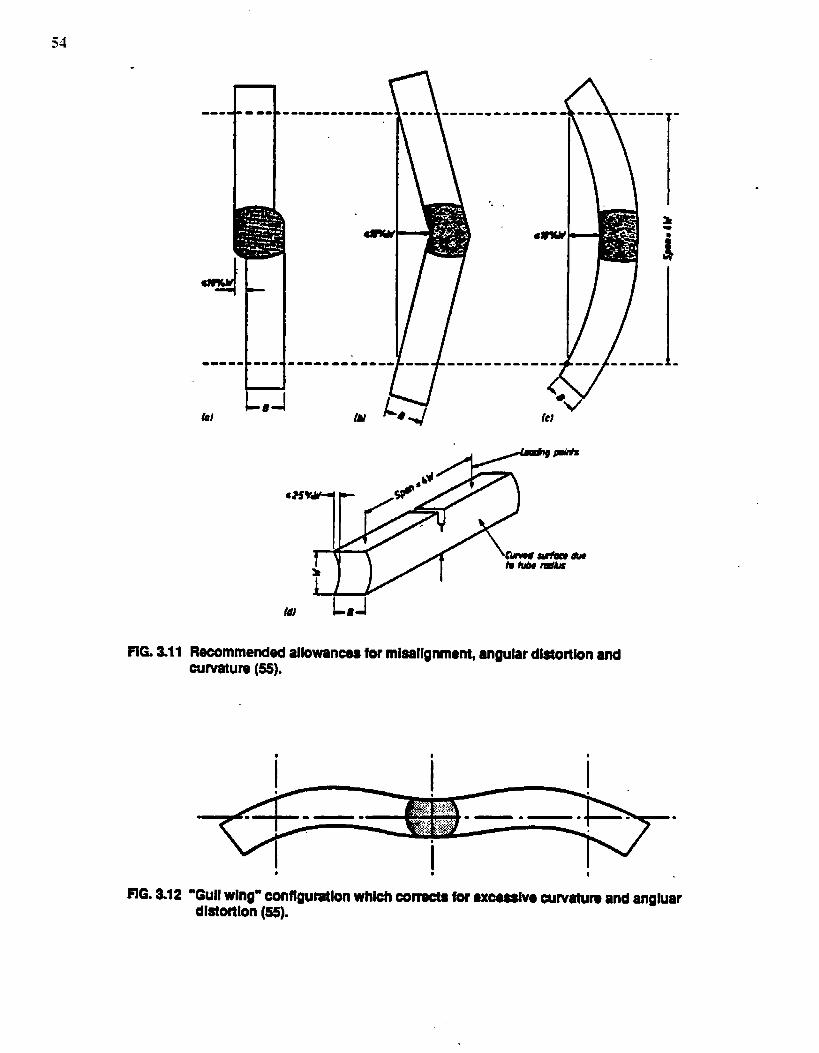
54

FIG 3.11

v 1

---- . - -. . . .. Z ---------

4!----------------------

4 I J!-—- ------ .. ----

4;

(t]/-

w Lmd

Recommendedalbwance.afor mlsallgnment,angulardla!ortfonandWlvature(55).

* #

I*

I. ,I

-—- -—.— . .w m,

I● * I

FIG.3912 “Gullwing”oonflgumtlonwhich oomcta for ●xcesslv- oumatureand angluardistortion(55).

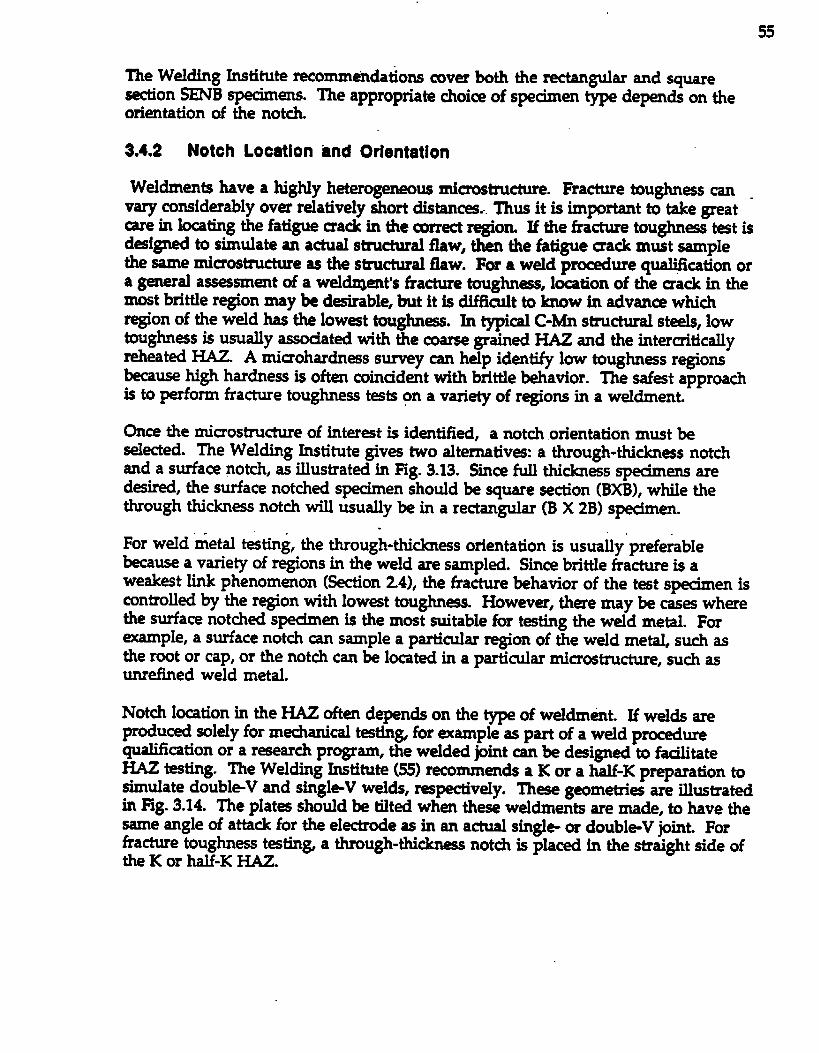
55

The Welding Institute recornrrwhdations cover both the rectamndar and sauaresection SENB specimens. me appropriate choice of spcirnen @ depend on-theorientation of the notch.

3.4.2 Notch Location and Orientation

Weldments have a highly heterogeneous microstnmture. Fracture toughnms can .vaxy considerably over relatively short distances... Thus it is important to take greatcare in kting the fatigue crack in the uwrect r@om If the fracture toughness -t isd=igned to simulate an actual structural flaw, then the fatigue sack must samplethe same microstnacture as the structural flaw. For a weld pr~ure qual@ation ora general -sment of a wel~ant’s fkactu.retouglums, location of the mack in themost brittle region may & d-able, but it is difkult to how in advance whichregion of the weld has the lowest toughn~. In typical C-Mn structural stAs, lowtoughn~s is usually assodated with the coarse grained W and the i.ntemiticallyreheated HAZ. A microhardn~s sumey can help identify low toughness regionsbecause high hardness is often coinadent with brittle behavior. The safest approachis to perform fracture toughness tests on a variety of regions in a wekl.ment,

Once the microstmcture of inter-t is identified, a notch orientation must beselected. The Welding Institute gives two alternativ~: a through-thickness notchand a surface notch, as illustrated in Hg. 3.13. Since full thickness specimens aredeired, the surface notched specimen should be square section (BXB), while thethrough thickn~s notch will usually be in a rectangular (B X 2B) spedrnen.

For weId “metal testing, the through-thickness orientation is usu~y preferablebecause a variety of regions in the weld are sampled. Since brittle fracture is aweskest link phenomenon (Section 24), the fracture behavior of the test specimen iscontrolled by the region with lowst toughn~s. However, there may be cases wherethe surface notched spednen is the most suitable for -ting the weld metal. Foracample, a surface notch can sample a particular region of the weld metal, such asthe root or cap, or the notch can be located in a particular mimostnwture, such asunrefined weld metal.

Notch location in the W often de~nds on the type of weld-merit. If welds areproduced solely for mechanical tdn~ for example as part of a weld pr=edurequaliikation or a research program, the welded joint can be d-igned to fadlitateHAZ testing. The Welding Institute (55) recommends a K or a half-K preparation tosimulate doubl&V and singl-V welds, rqectively. Thee geometxk are illustratedin Fig. 3.14. The plates should b tilted when these weldments are made, to have thesame angle of attack for the electrode as in an actual singk cmdoubl*V @nt. Forfracture toughness testin~ a through-thickn=s notch is placed in the straight side ofthe K or half-K W.

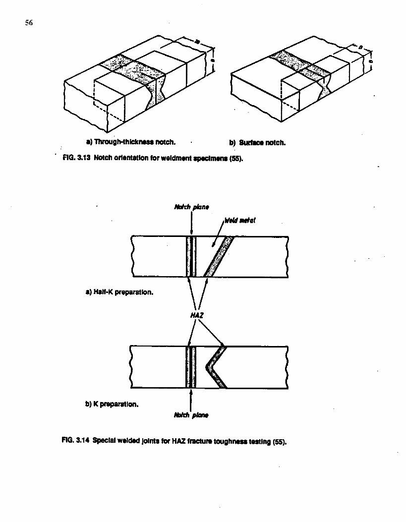
●) T?u’ough-thkkneesnotch. “ b) ~ tiCk

“ flG. 3.13 Notch orientation for weldment spsclmene (55).

MM phne

W Wal .

. ..

a) Half-Kpreparation.

\/

FIG.3.14 SpecialweldsdjointsforHAZfiaoturatoughnwatasting(35).

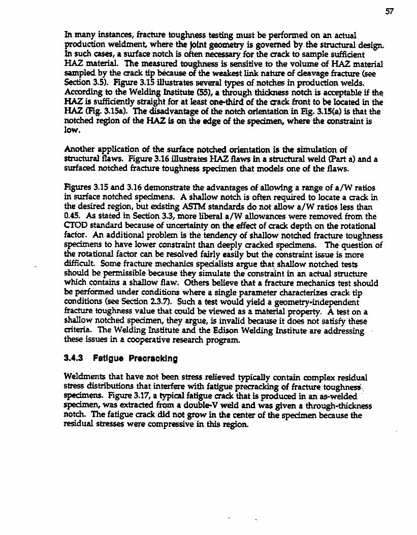
In many instances, fracture toughn=s tdng must be performed on an actualproduction weldment, where the joint gmmetry is governed by the structural desigmIn such cases, a surface notch is often necessary for the crack to sample sufliaentHAZ material. The measured toughness is sensitive to the volume of HAZ materialsampled by the crack tip kause of the weakest link nature of cleavage fra-e (seeSection 3.5). Hgure 3.15 illustrates several typs of notches in prmiuction welds.According to the Welding Institute (55), a through tM&nss notch is acceptable if theW is suffiaently straight for at least orethird of the sack front to be Imated in theH (13g. 3.15a). The disadvantage of the notch orientation in Hg. 3.15(a) is that thenotched region of the HAZ is on the edge of the spedmen, where the constraint islow*

Another application of the surface notched orientation is the simulation ofstructural flaws. Figure 3.16 illustra~ H#GLflaws in a structural weld (Part a) and asurfaced notched fracture toughness specimen that models one of the flaws.

Figures 3.15 and 3.16 demonstrate the advantages of allowing a range of a/W ratiosin surface notched specimens. A shallow notch is often required to locate a mack inthe desired region, but existing ASTM standards do not allow a/W ratios less than0.45. As stated in Section 3.3, more liberal a/W allowances were removed from theCTOD standard because of uncertainty on the effect of made depth on the rotationalfactor. An additional problem is the tendency of shallow notched fracture toughnesss@mens to have lower constraint than deeply cracked specimens. The qu~tion ofthe rotational factor can be rsolved fairly easily but the constraint issue is moredifficult. Some fracture mechanics speaalists argue that shallow notched testsshould be permissible because they simulate the constrht in an actual stnxturewhich contains a shallow flaw. Others believe that a fracture mechani~ test shouldb performed under conditions where a single parameter characterizes crack tipconditions (see Section 23.7). Such a test would yield a geometry-independentfracture toughness value that could be viewed as a material property. A test on ashallow notched specimen, they argue, is invalid because it does not satisfy theseaiteria. The Welding Institute and the Edison Welding Institute are addressingthese issues in a cooperative r~arch program.

3.4.3 Fatigue Precracking

WeIdments that have not been stress relieved typically contain complex residualstress distributions that interfere with fatigue precracking of fracture toughnesix-. ~~e 3.17, a typical fatigue crack that is produced hi ~ as-weldedspd.rnen, was extracted from a doubl-V weld and was given a through-thicknessnotch. The fatigue crack did not grow in the center of the specimen because theresidual stresses were compr~sive in this region.

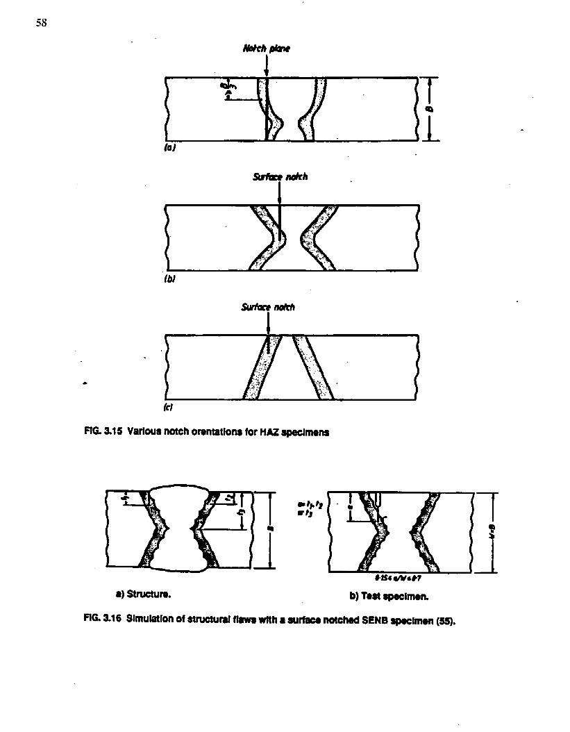
58

lb)

(d

FIG 3,15 VariousnotchorentatlonsforH= 8p#Mrn0~

8) structure. b) Teslspeclmmt.

FIG 3.16 Simulationof structuralflaws wtth● sum notchedSENBspeolrnon(S5).

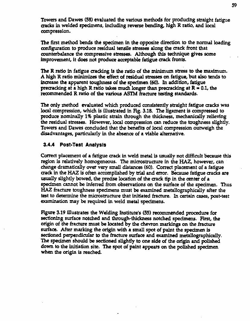
Towersand Dawes (58) evaluatedthe variousmetlds for producing straight fatiguecracks in welded spedrnens, including reverse lwwli.ng high R ratio, and localcompression.

The tit method &nds the specimen in the opposite direction to the normal loadingcm@u.ration to produce r-idual tensile stiesses along the =ack front thatcounterbalance the compressive str~~. Although this technique gives someimprovement it doss not produce acceptable fatigue uack fronts.

. .

The R ratio in fatigue cracking is the ratio of the minimum stress to the maximum.A high R ratio ~ the effect of =idual str~- on fatigue, but also tends toincrease the apparent toughn~s of the specimen (60). Jn addition, fatigueprecracking at a high R ratio take much longer than preuacking at R = 0.1, therecommended R ratio of the various ASIld fracture tdng standards.

The onIy method evaluated which prmiuced consistently straight fatigue sacks waslocal compression, which is illustrated in 13g. 3.18. The ligament is compr~sed toproduce nominally 1% plastic strain through the thickness, mechanically relievingthe residual stres~. However, kal compression can reduce the toughness slightly.Towers and Dawes concluded that the benefitsof local compression outweigh thedisadvantages, particularly in the absence of a viable alternative.

3.4.4 Post-Test Analysis

Correct placement of a fatigue crack in weld metal is usually not difficult because thisregion is relatively homogenaw The microstructure in the W, however, canchange dramatically over vey small distances (60). Correct placement of a fatiguecrack in the W is often accomplished by trial and error. Because fatigue sacks areusually slightly bowed, the predse location of the sack tip in the center of aspedmen cannot be inferred from obsemations on the surface of the spedrnen. ThusHAZ fracture toughness specimens must be examined metallographically after thetet to determine the microstructure that initiated fkacture. In certain cases, post-testexamination may be required in weld metal s@mens.

Hgure 3.19 il.lustra~ the Welding Institute’s (55) recommended procedure forsectioning surface notched and through-thidmess notched spedmens. First, theorigin of the fracture must be located by the chevron markings on the fracturesurfam After marking the origin with a small spot of paint the spedmen issectioned perpendicular to the fracture surface and examined metallographically.The spedmen should be sectioned slightly to one side of the origin and polisheddown to the initiation site. The spot of paint appears on the polished specimenwha the origin is reached.

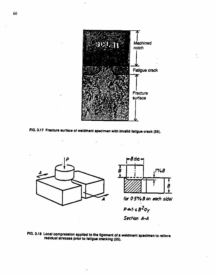
60

I crack

F&ture

surface

FIG.al? Fracturesutiaco of woldments~lmon wtlh Invalidfatlguocrock (58).

FIG.3.18 LocalcompnasslonappliedtothoIlgamwttof ●weldmentspaclmento mliewrasldualstressespriorto fatiguecracking(55).

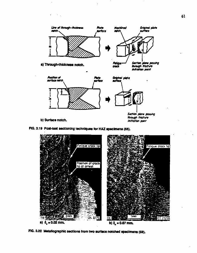
●Wouglwthkknm notch.

0.

S%zidI =** .\ i- \

PIG.3.19 Peat-tas!$actIoningtachnlquaafor HAZ ~lrnans (5S).

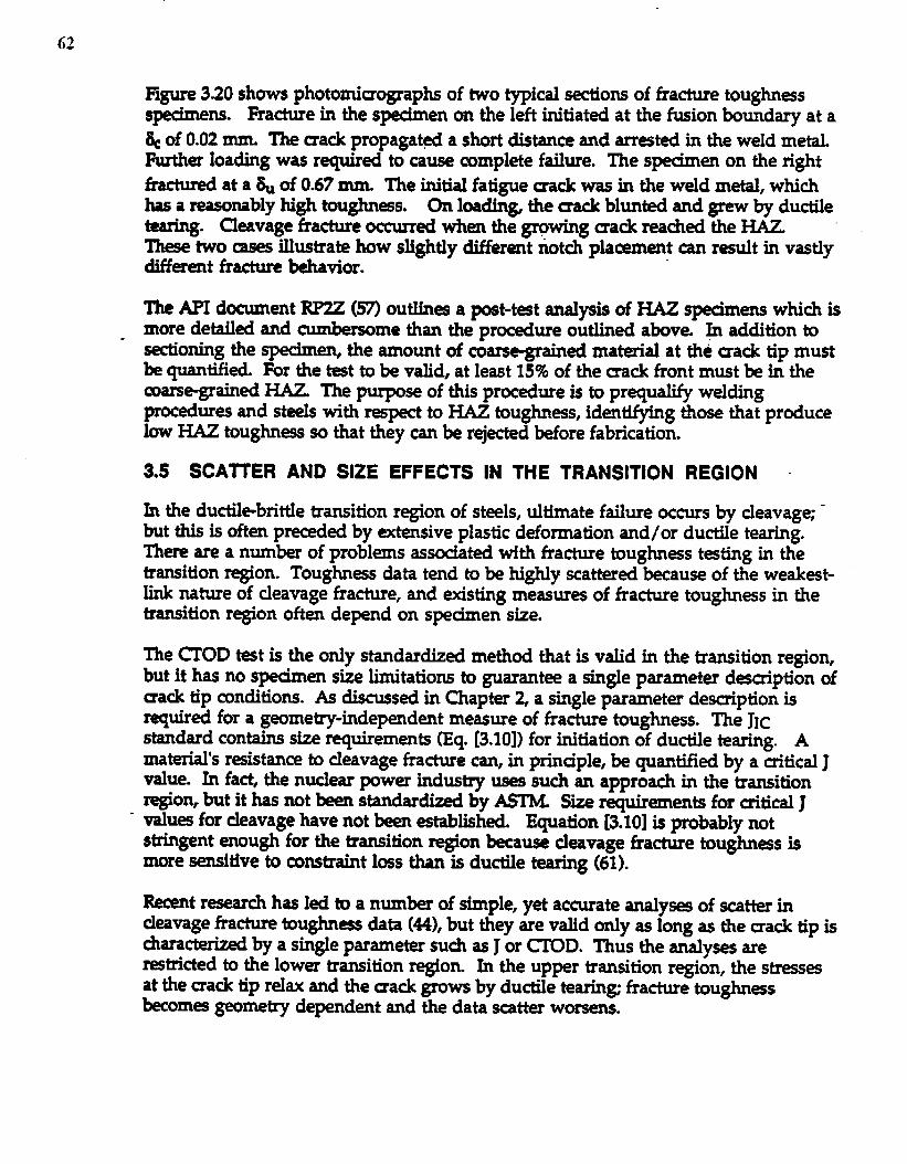
Figure3.20shows photomimographs of two typical sections of fracture toughn~ss@dmens. Frahe in the sxen on the i~ initiated at the fusion lm~dary at a~ of 0.02 mm. me crack propagat@ a short distance and arrested in the weld metal.Further loading was required to cause complete failure. The sped.men on the righttied at a ~ of 0.67 nun The initial fatigue sack was in the weld metal, whichhas a reasombly high toughna. On loadin~ the uack blunted and grew by ductiletearing. Cleavage fracture occurred when the growing sack reached the EWL ~Th#e two cases illustrate how slightly different riotdh placement can result in vastlydiffermt fracture &havior.

The API document ~ (57) outlirw a pst-t~t analysis of HAZ spcimens which ismore detailed and cumbersome than the procedure outlined above. @ addition tosectioning the specimen, the amount of coarsegrained matial at the crack tip mustb quantified. For the test to be valid, at least 15% of the sack front must be in thecosrsegrained U The purpose of this procedure is to prequalify weldingprocedures and steels with respect to HAZ toughness, identifying those that producelow HAZ toughness so that they can be rejected before fabrication.

3.5 SCA7TER AND SIZE EFFECTS IN THE TRANSITION REGION

In the ductil-bnttIe transition region of steels, ultimate failure occurs by cleavage; -but this is often preceded by ~tensive plastic deformation and/or ductile tearing.There are a number of problems associated with fracture toughness testing in thetransition region. Toughn~ data tend to be highly scattered because of the weakest-Iink nature of cleavage fracture, and existing measures of fracture toughness in thetransition region often de~nd on spedrnen size.

The ~OD tst is the only standardized method that is valid in the transition region,but it has no spedmen size limitations to guarantee a single parameter description ofmade tip conditions. As discussed in Chapter 2, a single parameter description isrequired for a geometry-independent messure of fracture toughness. The J1cstandard contains size requirements (Eq, [3.10]) for initiation of ductile tearing. Amaterial’s r~istance to cleavage fracture can, in prinaple, be quantified by a aitical Jvalue. In fact, the nuclear pwer industry uses such an approach in the transitionregio% but it has not been standardized by ASIIA Size requirements for ~tical Jvalu- for cleavage have not ~ established. Equation [3.10] is probably notstringent enough for the transition region kcause cleavage fracture toughnas ismore sensitive to constraint lms than is ductile tearing (61).

Recent research has Ied twa number of simple, yet accurate analy~ of scatter incleavage fracture toughn~ data (44), but they are valid only as long as the crack tip ischaractdzed by a single parameter such as J or CIUD. l%us the snalyses arer~tricted to the lower transition region. In the upper transition region, the stressesat the mack tip relax and the crack grows by ductile tearin~ fracture toughn~skomes geometry dependent snd the data scatter worsens.

63

3S1 Scatter In the Lower Transition Region

When an qerknental measurement displays a high degree of scatter, it iscustomary to attempt to reduce this scatter by =erdsing tighter control ov= theqeriment. Much of the obsemed scatter in cleavage fracture toughn=s data is aninherent feature of the material, however, that cannot be eliminated by improvingthe eqmimental procedure. Fortunately, fracture tough= scatter obeys certain .ruk and its magnitude can be predicted ‘.

Statidkd Aspects ~ FractureA nu.mbr of mkomechanical models for cleavage fracture have ken proposed inthe past few years(35~); all based on weakest link statistim. Each model relates amaterial’s miffostmcture to cleavage fracture toughness.

When fkacture wcurs by a weakst link mechanism, the failure probability is equal tothe probability of sampling at least one critical miaostructural feature. The Poissondistribution appropriately describes the failure probability in this - (43):

where F is the failure probability, V* is the volume in the process zone ahead of the=aclc tip, and

# particles 2 Uitical sizeP =

unit volume

‘The parameter p contains the inherent fracture propertk of the microstructure. Themaaosmpic fracture propertk of a structure or~~~ specimen can be obtained byintegrating p over the appropriate volume. In a uniaxial tensile specimen, p isconstant throughout the gage section if the stress is constant, but p varies with

position when a crack is print lxcause p depends on stress. The critical particle sizeis related to str~ through Eq. [231]. N str~s in~ , uiticzd size d~; P~ with str-s lwcause more partick are =pable of initiating cleavage.Andmn (43) modeled the str- dependen= of p with a modified pwer law

~=(W$llP

YE.IS]

where 61 is the maximum prinapal str~s at a point, and CU,m and v are materialconstants that characterize the fracture proprtk of the miaostructure. The

04

qusntity OUis the threhold stress, corrqonding to the Iarg=t conceivable particlein the material.

If fracture occurs by a weak-t link mecknism and the mck tip strm arecompletely charactdzed by J (e.g. Fig. 216a-b), it can & shown (44) that fracturetoughness data follows a characteristic distribution function

-. ..

‘=+-w]or

[3.19a]

[3.19b]

or

‘=1--R(3! [3.19C]

for uitical J, ~OD and K values, respectively; BOis a reference thicluwss. Thequantiti- 9J, es, and eK are the 63rd prcentile values of the coqesponding fracture

-toughness parameters when speamen thickness = Bo. Th-&e th.m cbnstants arerelated through Eqs. [226] and [228]. Equation [3.19] is derived in the Appendix. Anumber of investigators (44, 62, 63) have derived nearly identical cleavage fracturetO@IleSS distributions.

Equations [3.19 a-c] have the form of a Weibull distribution. The Weibull shapeparameter (or slope) =20 for uitical J and CTOD valus, and because of therelationship between J and K, the shape parameter = 4.0 for KIc or effective K valuescomputed from J (see Eq. [228]).

I&m 3.21 (M) gives an experimental validation of a thaxetied Weibu,ll sl~Experimental valu- of the Weibull slope from published-fracture toughness data areplotted as a function of data set size. All J and ~D data were converted toequivalent KIC values through Eqs. [226] and [228]. Although the computedWeibull slope are widely scattered for small sample sizes, the data approach thetheoretical value of 4.0 as sample size inaesses. The scatter in computed slopes canbe attributed to small sample effecis. The cum= in Hg. 3.21 represent 95%cotidence limits which were computed by Monte Carlo simulation. Finite sampleswere randomly taken from a hypothetical population of fracture toughness data witha true slope of 4.0, and Wei%ull SIO~ were computed. This process was repeatednumerous thn~ for various sample sk. Note that the Computed con.fldence limits

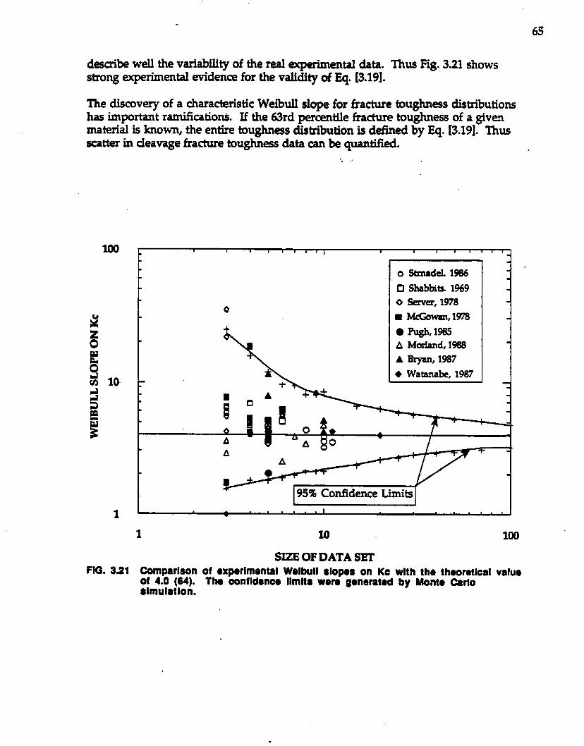
65

desuibe well the viability of the real experimental data. Thus Fig. 3.21 showsstrong qmixnental evidence for the validity of Eq. [3.19].

The discovery of a characteristic Weiiull slope for fracture toughnss distributionshas important ramificatioti. If the 63rd percentile fracture toughness of a givenmaterial is known, the entire toughn~s distribution is defined by Eq. [3.19]. Thusscatter in cleavage fracture toughn- data can IM quantied.

.. .,

1

\ +

O StmadeL1=O Shabbits.1%9o w, 1978■ -m, 19s

● Pugh,19s5A Mmlad, 1968A Brym, 19S7● Watana&,1987

SIZEOF DATA SErFIG. 321 Compsrlson of ●xperimental Welbull slopes on Kc with th. thaoretkal valu.

of 4.0 (64). The confld-noe Ilmlts were g.nersted by Mont. Carlosimulation.

Analysis of ScatterThe value of Eq. [3.19] can lx illustrated by introdudng two quantities thatcharacterize scattff. the confidence band ratio and the lower bound ratio. Themfidence band ratio is ob@ned by dividing the cofidence band width by themedian value. For example, the 80% cotidence band ratio for CTOD data is givenb’

[320]

Where b9, &I.1, md 60S are the 90% upper bound, 10%lower bound and medianCIOD valu~, r~pecdvely. Note that the con.iidence band ratio is independent oftemperature, specimen thickn~s, and material propertk. Although the scatter inabsolute terms increases with median toughness, the relative scatter is constant.

The Iower bound ratio is defied as the ratio of the median to a particular lowerlimit in the distribution. This is probably a more useful quantity than the CBRbecause the lower tail of a toughness distribution causes the most concern instructural applications. The 10% lower bound ratio is given by

Similarly, the 1% lower bound ratio can be computed

LBRo.01 =-=’.30

[3.21a]

[321b]

Thus, if the median ~OD is known, the 1 percent lower bound toughness can be=timated by ditiding the median by 8.30.

The con.tidence band and lower bound ratios would be identical for J and CTUD datasince lmth parameters have the same WeibuJl exponent, but K values have aWeibull exponent of 4.0, causing the data scatter to & somewhat different. Forexample, the 1 percent lower bound ratio for critical stress intensity data is given by

‘==(=Y’4=”‘Bm-O1 W.ol [321c]

Critical K data for cleavage appears to b 1ss scattered than J or CTOD data onlyWause Mh J and ~OD are proportional to Kz under small-scale yielding

..

67.

conditions. No benefit would ke realized by quantifying tougluws with K ratherthan J or CTOD. The uncertain~ in uitical crack size calculations that results fromtoughness S=tter is the same regardless of the fracture parameter.

Analysis ofSmull Data SetsEquations [3.20] and [3.21] ~timate relative scatter, but to det~e absolute valuesin the distribution with these e@ations, a single value (e.g. the median) must kknown. Stated another way, at least one point on the distribution must be known ~order to compute 6 and thereby dehe the entire distribution The degree of--tiwM& Om&~tiW d~&atitidtie aWbh&a~L

h most cases, a relatively small-number of fracture toughness *ts are u$ed toCharacttie a given material at a ~nstant temperature, pardy hcause fracturetoughness testing tends to h expensive and time consuming. In additio~ many stillview fracture mechanb analysis as determines tic; i.e., a single value of toughness istypically d to =timate aitical crack size. Consequently, large fracture toughnessdata sets are often unavailable

Stienstra et al. (64) developed an approach for infeming useful information fromsmall fracture toughness data sets by utilizing order statisth to estimate a lower-bound toughn~s value from the available data. The analysis assure= that Eq. [3.19]describes the toughness distribution. The lower-bound value is related to measuredvalu= by a multiplying factor. For example, the 10% lower-bound ~OD is=timated with 90% confidence as follows.

bl,O.9 = kO.1~.9(n)k [322]

where ko.l~.g(n) is a multiplying factor, n is the sample size, and ~n is the lowestCTOD in a set of n values. Whenever statistical inference are made from limiteddata sets, two probability valu= must be s@@d. The above equation mrrespondsto an estimate of the 10% lower bound for the toughness distribution. This is aconsa’vative estimate because the tie 10% lower bound lies above the =timate 90%of the time. Table 3.1 lists multiplying factors for four combinations of cotidencelevels and lower bounds This approach to lower lmund estima~ has a built-inretest rational, as illustrated in the following example.

Consider a set of three CTOD vah.ws for a given material, with ~ = 0.10 mmAccording to Table 3.1, the 1!)% lower bound, dmated with 90% confidence, is 0.037mm. Imagine a hypothetical application where ~-1~,9 must b at least 0.05 mm.Given the edsting data, one must conclude that the material’s toughness isinadequate for the application. However, additional t~ts may reveal that thema- is acceptable and that the low CTOD value in the first three ~ts was a rarity.

68

.

If a total of seven tests are performed and ~ remains at 0.10 mm, the 4.matedlower bound inaeases to 0.057, which is almve the minimum acceptable value.

The use of small data sets to =timate lower Ixmnd valu= is not without rest. Xnorder to obtain 90 or 95% mfidence that the ~timate is blow the true value, the@imate must be co~ative when the sample S* is small. In gen=al, theestimate is 1- consenative if more data are available (64). Thus there h a trude~.between the cmt of performing a large number of jhcture toughness t~ts and thecost of rejecting a rnateriul that may be adequate for the Upplicafion.

TABLE 3.1. Muttiplylng factom for ~imatlng 10wQrbound toughnoas fnmsmall data sats(64).

NUMBER OF MULTIPLYING FACTOR i)VALID 10’%Lower Bound 5% kWer Bound

90%Cofidence 95%Cofidence 90%Cofidence 95%Cor@dence

3 0.3705 0.3248 0.2585 0.22665 0.47$3 0.4193 0.3337 0.29267 0.5660 0.4%2 0.3949 0.346210 0.6764 0.5930 0.4720 0.413815 0.8205 0.7260 0.5781 0.506820 0.9566 0.8387 0.6675 0.5352

Thickness EfecfsThe weakest link nature of cleavage leads to a SW dependence on fracturetoughness. This is apparent from Eq. [3.19] because thickness appears in the~nen~ For a constant failure probability, critical J and C1’OD valu= are

proportional to l/@, and KIC (or wf) is proportional to B-it? Early studk (7, 65)on the size dependence of critical K valu~ concluded that a plateau value is reachedabove a critical thi~s, but the statistical model predicts that average K1c demasesby 16% eadh time thickness is doubled. Early immtigators probably lacked suffiaentdata to detect the continual decrease in toughnss. Statistical thickness effects can bemasked by the scatter in toughness.

Umdes and Schaffer (66) were the first to apply a weak~t-link statistical argument torelate fracture toughness data from large and small spe~ens. T&y fit Weibulldistributions to small specimen data and ~timated the average toughness of largespecimens with the following relationship:

69

(vsmall llPAvg. KIC we -) = Avg. KIC (small- x G [323]

where ~ is the WeibuJl slop The Landes and S&aHer analysis of thickness effects issimilar to Eq. [3.19], except they left the Weibull slop as a variable. ‘l’he discov~ ofa characteristic Weibull slop for cleavage toug~.ess (44, 62, 63) came wer~ years -after the brides and Schaffer study.

,.

S@mens@ effects on fracture bughness cannot always lx explained mmpletely byweakest link statisti~. When fracture is preceded by large scale plastia~ or ductiletearin~ additional size effects are obsemed (67), as dkussed in Section 3.5.2

Threshold ToughnessThe decrease in toughness with increasing thickn=s does not continue indetlnitely.Fracture toughness data dtibit an absolute minimum that is almve zero (62, 64).One reason for this is that the fatigue preuaddng procedure intrdu- warmprestress effects at the crack tip. The plastic zone forrped during pr=ac.king resultsin compressive residual str=s= when the specimen is unloaded. When thespecimen is reloaded at the tmt temperature, th-e stress must be overcome forfracture to occur. The compressive residual stresses can be represented by a negativestress intensity that reduces the effective KI:

&ff=KI-& [324]

where K1is the apparent stress intensity, and & is the stress intensity of thecompressive residual stmses. Equation [3.19c] can be modified to account for warmpr=tress effects

[32s]

‘Ihus ~ represents the thr=hold toughness for the material, analogous to the

thr-hold AK caused by crack closure effects during fatigue.

Experimental arid theoretical estimates of ~ indicate that it is approximately 20

MPa~for steels. The temperature dependence of ~ is unclear. Current -archat Texas A&l University is establishing more accurate ~timates of ~.

The “threshold toughn~s sigrMcantly influences the toughness distribution only onthe lower shelf, where the average toughn~ is of the same order as ~. In thetransition region, ~ can be neglected for most analyses. Unless otherwise specified,~ is assumed to equal zero in this document, and the cleavage fracture toughnessdistribution is desuibed with Eq. [3.19].

70

bcal Brittle ZonesSome materials contain Iodized regions of low toughness. Since cleavage fractureis a weak=t-link phenomenon, these local brittle zones (LBZS) can dominate thetiactu.re process. “

The most common instance of kal brittle zones is in the heat-affected mne (HAZ) .of a SW weldment (60, 68, 69). A typical weld HAZ contains a wide range ofrnicros&uctures because of the various thermal treatments encountered. Forexample, the material at the fusion lnmdary qerkms a very high austenitizingtszn~ature and cooling rate, while material a short distance away is subjected to amuch lower temperature and cooling rate. In addition, certain regions are temperedby sukquent welding passes. %me of the microstructure t produced are extremelybrittle.

The fracture Navior of such materials is compl~. The crack tip in a fracturemechank specimen is likely to sample a number of mimostructural regions. Thefracture toughness distribution depends on the relative volume of eachmicrostmcture that is sampled.

The statistical model desmibed above is capable of characterizing fracture toughnessdistributions in composite miaostructures SUA as weld HAZs. The contribution ofeach mimostructural region to the failure probability can be summed to obtain anoverall probability of failure. For example, if p constituent microstructure aresampled by the crack tip, the ~OD distribution is given by

[326]

where ai is the fraction of the ~ack front that samples the microstructural

constituent, and ei is a characteristic toughness for the constituent. Note that CTODstill follows a Weibull distribution with the slop= 2 Equation [3.26] redu~ to Eq.[3.19b] Wkl p = 1.

Consider a dupl= (p=2) microstructure with local brittle ~nes in a matrix that isthree tim~ as tough as the LBZS (iie., 91 = 902). 13gure 3.~ is a plot of normalhedCTOD versus percent LBZ(44). The median CR3D decra with increasing volumefraction of LBZ Beyond 40 ~rcent LBZ, however, the rate of deuease in toughness -is small. Figure 322 includ~ plots for matrix/LBZ toughn~s ratios of three, ten, andinfinity. The tune for toughness ratio = 10 is ssentially identical to the mmecorresponding to an infinitely tough matrix Th.is implies that a constituent tenties as tough as the most brittle constituent does not contribute to the overall

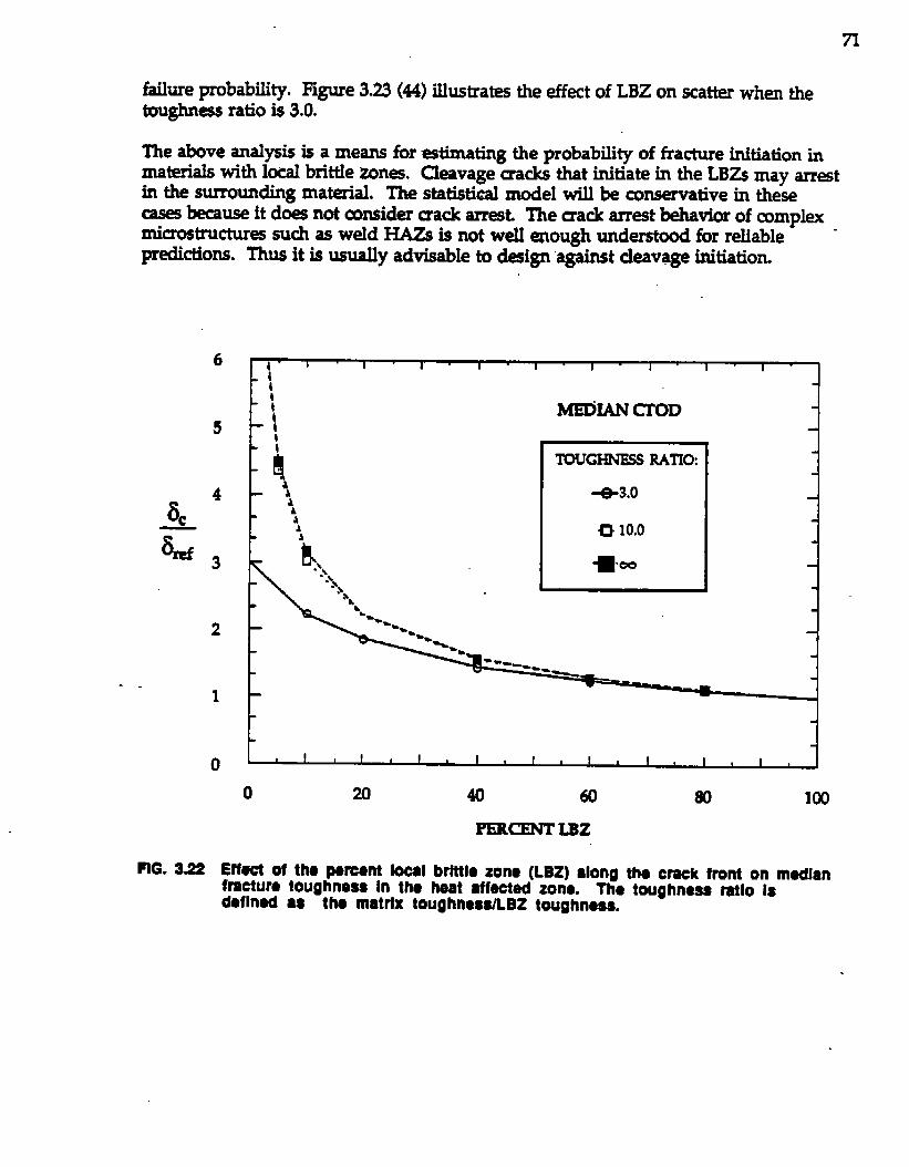
n

failure probability. R&e 3.23(44) illustrates the effect of LBZ on scam when thetoughn=s ratio is 3.0.

The a~ve analysis is a means for drnating the probability of fracture initiation inmaterials with Icxal brittle nn~. Cleavage macks that initiate in the LBZS may arrest

umoundi.ng material. The statistical model will be consemative in theseinthesu kause it doa not consider sack -t The mack arrest behavior of complexmicrostrum sudi as weld ~ is not well enough understood for reliable -predictions. Thus it is usually advisable to design against cleavage initiation

6

5

& 4k 3

2

._1

0

FIG. 342

t i

1 * I I I , 1 I I 1 I I I I 1

0 20 40 60 m lcm

PERCENT IBz

Efkt of the psrcont local brtttls zono (LBZ) ●long tho crack front on madlanfmeturo toughness in ths heat affactad zorm. Tho toughness rstlo iadoflnad as ths matrix toughn8asLBZ toughness.

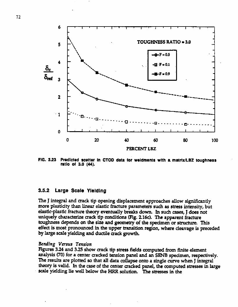
72

&

ad

6

5

4

3

2

1

0

1 I 1 I I I I I I I 1 I Ii

Ii 1

i I

\

+

TOUGHNESS =TIO = 3.0\\\

“’m,,

El. ‘:

+F =0.5

% -E F= 0.1.. ..

“’IL.% ~~F =0.9 “.*W

‘-=----- -9- -B- . -------

--- -““”~ . . ...=

u.- +...

a----- ------ “a-------------------

I I I I I a 1 J 1 I I

0 20 40 60 $0 100

PERCENT LBZ

FIG. 333 Predicted aoatter In CTOD data for weldments with a matrix/LBZ toughness “ratio of 3.0 (44).

3.5.2 Large Scale Yielding

The J integral and mack tip opening displacement approaches allow significantlymore plastidty than linear elastic fracture parameters such as str~s intensity, butelastic-plastic fracture theo~ eventually breaks dowm In such cases, J d- notuniquely characterize crack tip conditions @lg. 216c). The apparent fracturetoughn-s depends on the size and geometry of the spednw.n or structure. Thiseffect is most pronounced in the upper transition region, where cleavage is preceded@ ~e scale yielding and ductile uack growth.

Bending Versus Tension@r~ 3.24 and 3.25show sack tip sfress fields computed from finite elementanslysis (70) for a center cracked tension panel and an SENB specimen, r~pectively.The results are plotted so that all data collapse onto a single -e when J integraltheory is valid. In the case of the center cracked panel, the computed stzess= in largesude yielding lie well below the HRR solution. The stresses in the

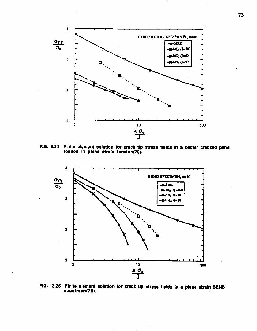
73

4

3

2

1

-.❑

1 10

x 00

J

FIG. 3.24 Flnlte element solutlon for crack tlp stressloaded In plane strain tension.

3

2

1

FIG. 345

la)

fields In a center cracked panel

1 lm

Finite element solution for crocktlp stress fields In a plane stmln”SENBspecimen. -.

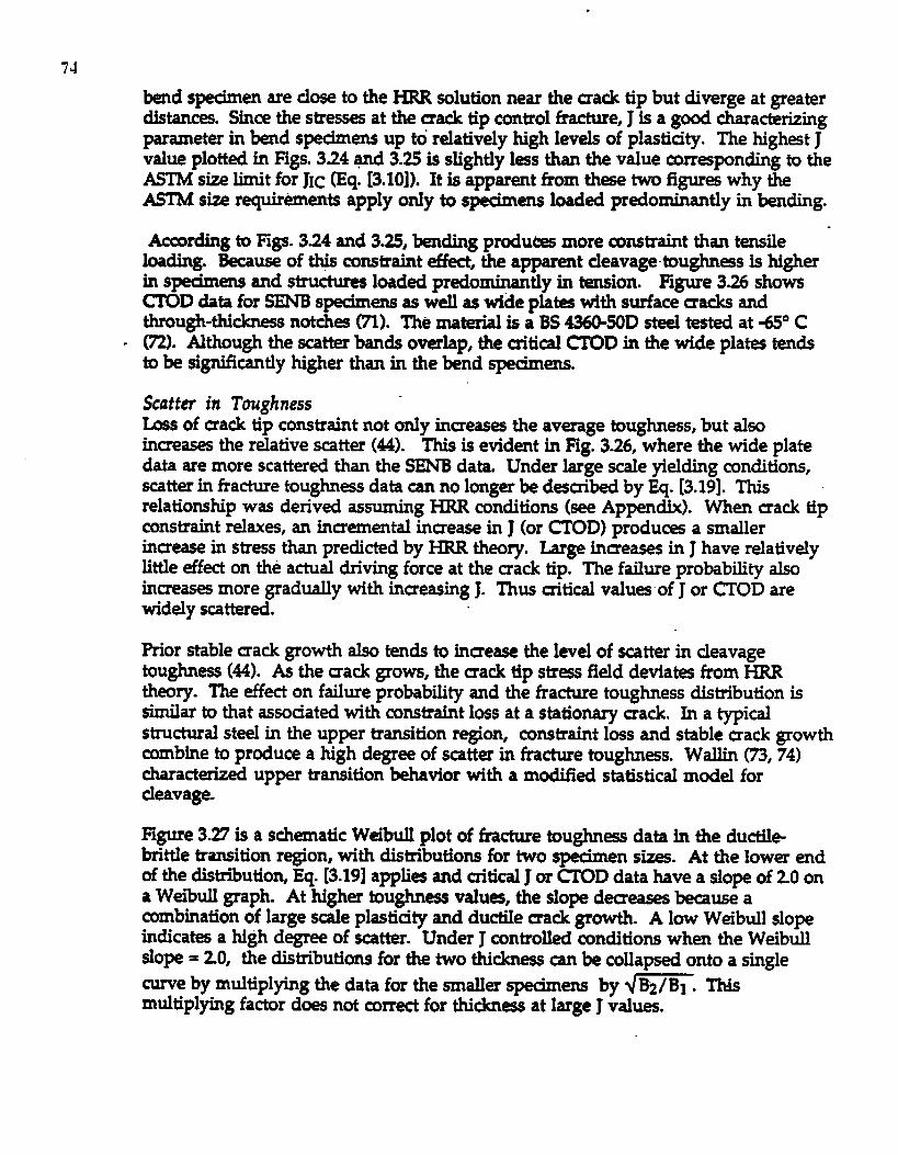
74

bend specimen are close to the HRR solution near the sack tip but diverge at greaterdistant=. Since the stresses at the mack tip control fracture, J is a good characterizingparameter in bend spedmens up to relatively high levels of plastiaty. The highest Jvalue plotted in Figs. 3.24 Wd 3.ti is slightly 1-s than the value corr=ponding to theASTM size limit for JIC (Eq. [3.10]). It is apparent from these two figures why theASTM size requir&ments apply only to s@nwns loaded predominantly in bending.

According to figs. 3Q4 and 3.25, haling prcdu~ more constraint than tensile -loading. Because of th$s constraint effect, the apparent cleavagetoughn~s is higher

minantly in tension. Hgure 3.26 showsin spedmens and structures loaded predoCTOD data for SENB specimens as well as wide pla~ with surface mdcs andthrough-thickness notch= (71). Tf@ material is a BS 4360-SOD steel tested at 4S0 C

- (72). Although the scatter bands overlap, the titical CTOD in the wide plat- tendsto be signii5csntly higher than in the bend spednwns.

Scatter in Toughness -Loss of crack tip constraint not only incre~ the average toughness, but alsoinaeases the relative scatter (44). This is evident in Hg. 3.26, where the wide platedata are more scattered than the SENB data. Under large scale yielding conditions,scatter in fracture toughness data can no long= be described by Eq. [3.19]. Thisrelationship was derived assuming HRR conditions (see Appendix). When ~ack tipconstraint relaxes, an imnrnental increase in J (or CTOD) produ~ a smallerincrease in stress than predicted by HRR theory. Large in~eases in J have relativelylittle effect on the actual driving force at the mack tip. The failure probability alsoincre~ more gradually with increasing J. Thus aitical valu~ of J or CTOD arewidely scattered.

Prior stable crack growth also tends to increase the level of scatter in cleavagetoughness (44). As the crack grows, the crack tip stress field devia~ from HRRtheory. The effect on failure probability and the fracture toughness di.stibution issimilar to that assoaated with constraint loss at a stationary crack. In a typicalstn.wkuralsteel in the upper transition region, constraint loss and stable crack growthcombme to produce a high degree of scatter in fracture toughness. Wallin (73, 74)characterized upper transition khavior with a modikl statistical model forcleavage.

I%gure3.27is a schematic Weibull plot of ticture toughn~ data in the ductilebrittle transition region, with distributions for two spedmen s*. At the lower endof the distribution, Eq. [3.19] appli~ and aitical J or ~D data have a slope of 2.0 ona Weibu.Ugraph. At higher toughness valu~, the slope decreases because acombination of large scale plasticity and ductile cradc growth. A low Weibull slopeindica~ a high degree of scatter. Under J controlled conditions when the Weibullslope = 20, the distributions for the two thickness can be collapsed onto a singletune by multiplying the data for the smsller spedmens by ~~. Thismultiplying factor d- not mrrect for thickn~ at large J values.

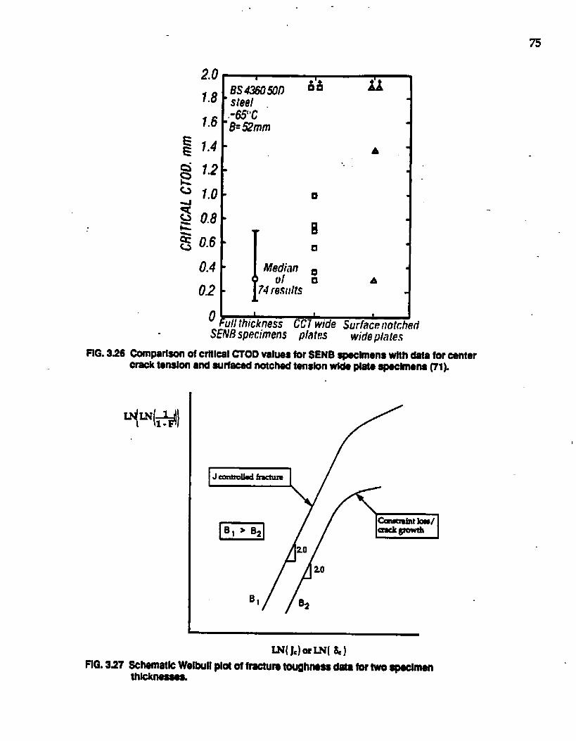
75

2.0

1.8

1.6

1.2

I*O

0.8

0.6

0.4

0.2

0

4.

13S4WSO17&’& Alsteel .-WC8=52mm

A..

●

Q

A

1 I * IIll thickness CC7 wide Surface notchedH specimens pL3teS wide plates

flG. 346 Oomparkonof critl~l CTODvsluss for SENBspecimenswith data for oentercrack tonslonand surfsesdn~ch8d tensbn wids plstespsclm8ns (71).

FIG.327LN(J=)orI,N( &)

Schernstk Wellwllplot of frsctm toughnossdata for two ap@tnanth~

76

Constraint loss and crack growth prmluce a thiclmess depndence in addition to thatassodated with statistical sampling effects.

Size E@ctsSize effects on fracture tou@nss in the transition region can be =used by acombination of constraint and statistical sampling effects. Figure 3.28 is a schematicplot of median fracture toughn- versus spedrnen size If the spci.men is largeenough to maintain J-controlled conditions, the size dependence of toughness is duemly to statistical effecls. The effect of thickn~ can b inkrred from Eq. [3.19]. Forsmaller sizes, the loss in sack tip constraint produc~ an additional size dependence,as indicated by the shaded area in Fig. 328.

The statistical size dependence on fracture toughness cannot be avoided, but it hssbeen quanti.ikd (Eq. [3.19]). Thus it is relatively easy to mrrect for Statistical effectswhen amalping a flaw in a structure. Since there are currently no provencorrections for sack tip constraint, J and CTOD tests in the transition region shouldbe @orrned on sufliaently large specimens to ensure J controlled conditions at themack tip. The minimum size requirements for cleavage toughnms have not beenestablished. The development of such criteria should be the subject of futurer=earch.

Comections for Crack Tip ConstraintIn certain instances, it may not be practical to perform a fracture toughness t~t underJ controlled conditions. For munple, an engineer may want to test a specimen witha shallow mack @ order to simulate a surface flaw in a structure. In such cases, the

- resulting fracture toughness will be influenced by constraint loss. Although thereare no proven methods to correct for constraint loss, a receqtly developed analysisshows some promise. Anderson derived a J-like parameter to characterize thestress normal to the sack plane (~) under large scale yielding conditions

Red that dn is a dimensionless constant that relat~ J and CTOD under HRRconditions (Eq. [226]). Equation [3.27J characta the 10SSin triaxiality through thechange in the J-CI’OD relationship from the HRR SOlutia. Wien the HRR solutionis valid, JW’ = J. Figure 3.29 shows the Wte element results from Fig. 3.24,normalized in terms of Jm” rather than J. Tl@ new psrameter appears b correct thestr~s fields for constraint loss. Since ~ nesr the sack tip governs cleavage, J ●

Pcan be viewed as the effective driving form for cleavage. Further validation o thisparameter is needed before it can be applied to practical situations.

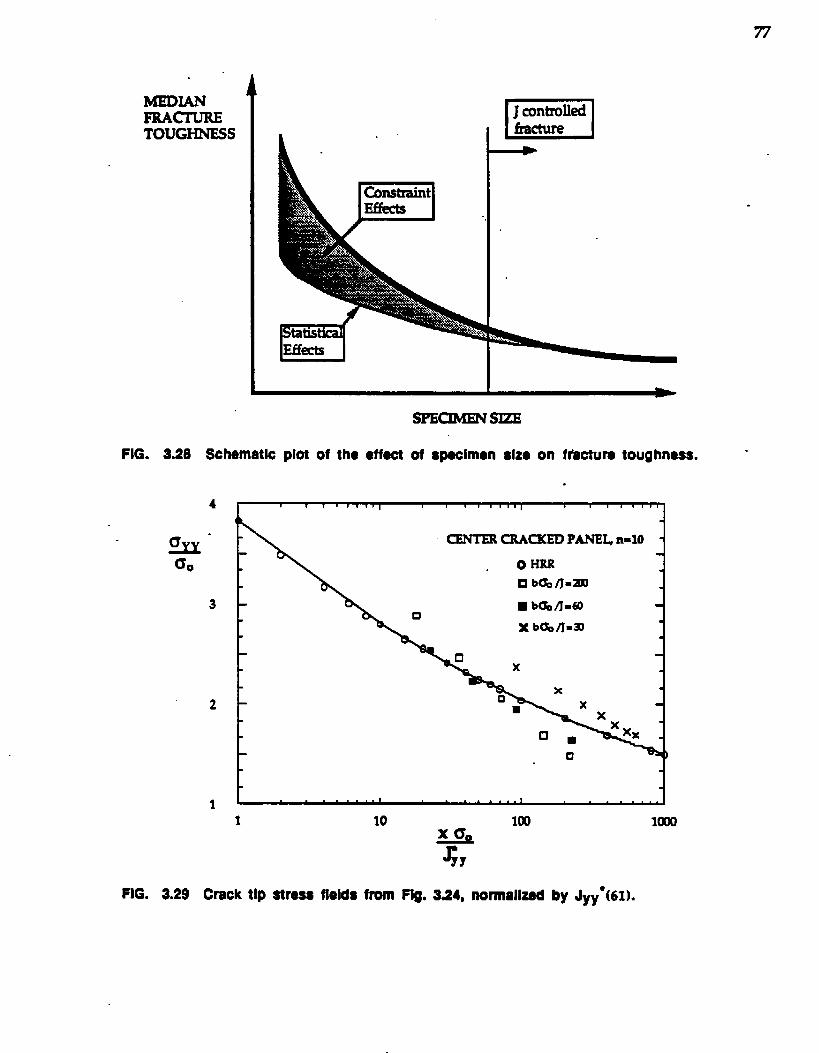
MEDIANFMCT’URETOUGHNESS w

SPECIMENSIZE

FIG. 3.28 SchematlC plot of the ●ffect of specimen size on fktima toughness. -

.

1 1 r 1 I 1 [

xL x

2

11 10

FIG. 3,29 Cracktlp stress fields from Fig.

JYY

3s4, normalized

lam

by JYY*(61).

3.6 DYNAMIC FRACTURE TOUGHNESS AND CRACK ARREST

Mwn fracture is associated with either a high loading rate or a rapidly propagatingcrack, the probkn is complicated by two facto= the inertia of the stmcture and thestrain rate seiwitivity of the material. With inertia effects, calculation of uack tipparameters such as J and K is much more difficult (75). When the strainrate variesover several orders of magnitude, metals behave in a viscoplastic manner, even atlow temperatu.r~. A material’s flow s&-s inu- with strain, rate; thus quasistatictensile properti~ are not relevant at high strain rates. .

The relationship between loading rate and fracture toughness is compl~ Inertiaeffects tend to increase the apparent toughness of the material because the totalfracture energy includ~@gniiica.nt kinetic energy component Viscoplasticmattial Mavior can either inmease or decrease the toughmm with loading rate,depending on the fracture mechanism. Cleavage fracture toughness tends tod-ease with strain rate because cleavage is str~s controlled. Increasing the flowstress makes it easier for material at the uack tip to reach the critical cleavage stress.Since mimovoid coalescence is predominantly strain controlled, upper shelftoughness usually incre~ with strain rate. As the flow str~ increases, moreenergy is required to deform the material near the ffack tip to a critical strainDuring rapid propagation of a mack in a large specimen or structure, the mack speed(and hence the local strain rate) can vary considerably. In such case it is not unusualfor the fracture mechanism to alternate between cleavage and ductile tearin~ as onemechanism becomes more favorable than the other (76).

Inda effects are most pronounced immediately after application of the load (~.The material oscillates as stress waves propagate through the specimen, and theamplitude of these oscillations d-eases rapidly. Mter a short time, the local inertiaeffects are small and the behavior is dominated by global inertia effects. At long-, the &havior of the specimen is similar to that of the quasistatic rose, with the=ception of viscoplastic material flow properties. Nakamu.ra et aL (77) developedthe concept of a transition time, tT, to delineate between short time response, whereinertia effects are important, and long time khavior, where inertia effects are smallrelative to the total energy in the specimem Dynamic finite element analysisprformed by Nakamura et al. indicates that inertia effects are small at times greaterthat 2@. As long as &acture initiation occurs after 2tT, the dynamic JXCcan kcomputed from the quasi5tatic relationships in ASTM E613-87..

Joyce and Hacket (78, 79) have applied the transition time concept to dynamic Jtdng. They have perfected experimental tedniques for high rate fracturetoughnes ~ts on SENB specimens. Th~ sped.mens are typically 25 mm thick andare heavily instrumented. Impact loading is applied by a drop tower. Nakamura etaL estimated the transition time for these spedmens to be 300 W. Materials thatJoyce and Hacket have tested are relatively ductile. Fracture initiation in th-materials usually oc~ between one and two milheconds after the tup contacts thespecimen. Siice the time to fracture is greater than 2~ in this case, J can be

79

computed with Eqst”[3.5] to [3h7a]. Joyce and Hacket developed a key cum method toinfer sack growth during the t~~ Hgure 3.30 (78) compares quasistatic J-R cunws fora 3-Ni st-1 with dynamic cumes obtained from the their method. The Viscoplasticmatdal behavior causes the matetial ~istance to imxease with strain rate, asqed.

When inertia effects are minimal, dynamic loading reduc- cleavage fracturetoughness. Since plastic deformation in steels is ,a thermally activated process, “increasing the strain rate is equivalent to ~tfng at a lower temperature. Thus, whenthe loading rate inue~, the ductikbritt,le transition tune shifts upward in@nperature. For example, Hg. 3.31 shows fracture toughn~s data for an A572 Grade50 sM at three loading rates (80). ‘The transition CUXVMshift approximately 2008F(ll~C) betw= the low=t and highest strain rate.

Once cleavage initiates, whether from quasistatic or dynamic loading a propagatingcleavage crack moves rapidly through the spedmem Material near this propagatingcrack is subjected to very high strain rates. Thus the situation is analogous to acontinuous dynamic fracture toughnss test. In order for the crack propagation tocontinue, the driving force for fracture must be at least as large as the materialreistance. Resistance of a steel to cleavage fracture can be represented by a falling Rawe, as illustrated in Fig. 3.32 When fracture initia~ at K1c, the crack propagatesin a rapid and unstable manner. The @acture process then becomes dynamic, andresistance to cleavage deaeases. In many loading situations, the driving forceinmeas= with crack length or remains constant, and the mack continues topropagate. In some c-, however, the driving force may decrease until it intersectsthe material resistance tune, and the crack anests because further propagation isimpossible. The arret toughness, KIWis a measure of a material’s ability to stop arapidly propagating aak

There a number of practical situations in which mack arr~t can occur. A sped.menor stnmture loaded in displacement control can have a falling driving force cume. Afalling driving force cume can slso result from a transient load, as when a shipcollides with another v=sel. The transient load may be sufficient to initiatecleavage, but the driving force decreases rapidly as the stress wav~ are damped bythe structure. bother common scenario for ~ack arrest involves a toughnessgradient For ewnple, a crack may initiate in a cold region of a stnxture, wh~e thetoughxuss is low, and propagate into material at a higher temperature snd toughn~skveL The sack am~ts when the K~ exceeds the driving force. A toughnessgradient could also radt from variations in microstructure, SUA as in weldedstructures. If a cleavage crack initiates in a brittle region of the weld, it may arrestwhen it reach= the parent metal, whidi usually has higher toughn~s.

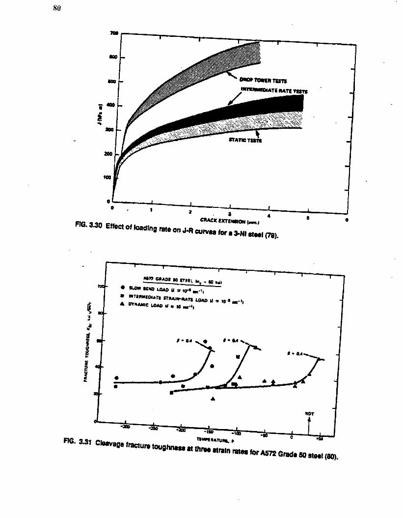
80

m. 330

OL 1 I0, 1

I

zI I

3 AI

cn&REWE~(-, “ s

Effectof Ioadlngrateon J+ CUIWSfor a $Nt at~l (78).

. ●

*

9 ●

A

6

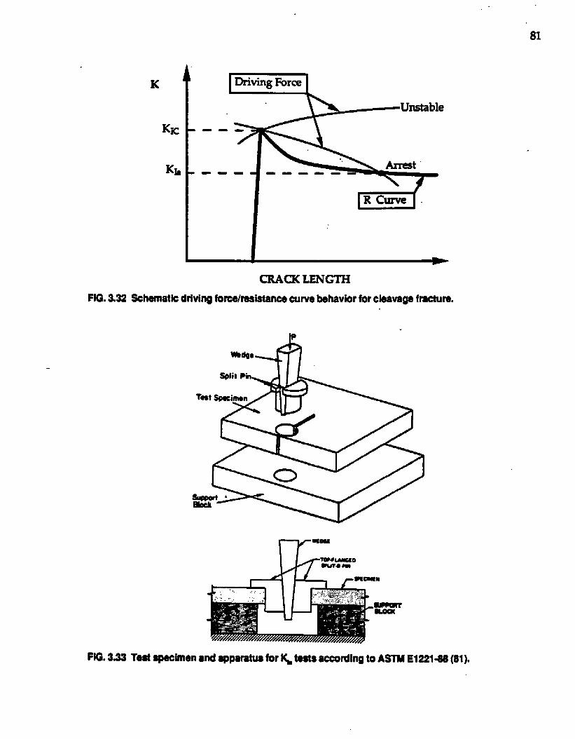
K

KIC

K~ .---,

CMCK LENGTH

FIG.333 Schamatkdrivingforca/resktancecumebshavforforcbavaga fmctura.

rr-

Fffi. 333 Teaf apacimon●nd apparatuafor ~ teals acoordlngto Am E133W8 (81).

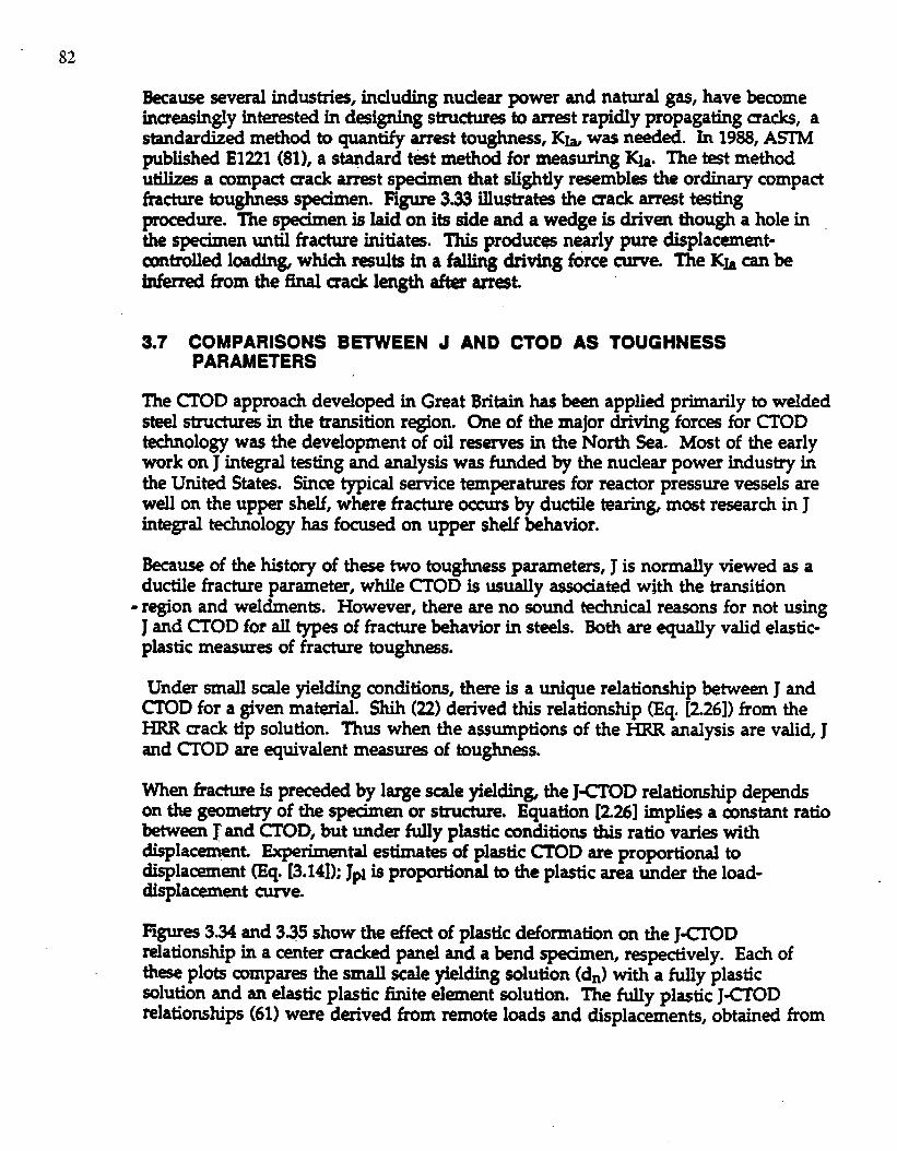
82

Because several industrie, including nuclesr pwer and natural gas, have bcomeincreasingly interested in d-igrd.ng stnxtures to arret rapidly propagating cracb, astandardized method to quantify arr=t toughness, Kk was n~ed. In 1988, ASTMpublished E1221 (81), a st~dard test methti for measuring Kh. The -t methoduiilizes a compact mack ~t spedmen that slightly r-mbl- the ordinary compactfracture toughrms specimen. Figure 3.33 illustra= the sack arrest ~tingprocedure. lhe specimen is laid on its side and a wedge is driven though a hole in .the s@men until fracture initiat=. This prdw~ nearly pure displacemmt-con~lkd loadin~ which -ulti in a falling driving force tuna The K~ can beinked from the final uack length after arr~t

3.7 COMPARISONS BETWEEN J AND CTOD AS TOUGHNESSPARAMETERS

The ~OD approach developed in Great Britain has been applied primarily to weldedsteel stictur= in the transition region. One of the major driving forces for CTODtechnology was the development of oil r-emm in the North Sea. Most of the earlywork on J integral testing and analysis was funded by the nuclear power industry inthe United States. Since typical semice temperatures for reactor pressure v~sels arewell on the upper shelf, where fracture occurs by ductile tearin~ most research in Jintegral technology has focused on upper shelf behavior.

Because of the history of these two toughness parameters, J is normally viewed as aductile fracture parameter, while ~OD is usually associated with the transition

- region and weldrnents. However, there are no sound technical reasons for not usingJ and CTOD for idl types of fracture behavior in st~. Both are equally valid elastic-plastic measur~ of fracture toughness.

Under small scale yielding conditions, there is a unique relationship between J and~D for a given material. Shih (22) derived this relationship (Eq. [2.26]) from theHRR mack tip solution. Thus when the assumptions of the HRR analysis are valid, Jand CTOD sre equivalent measur= of toughness.

When fracture is preceded by large scale yieldin~ the J~OD relationship depadson the geometry of the spedmen or structure. Equation [226] implies a constant ratioWeen J and CI’OD, but under fully plastic conditions this ratio vari~ withdi.spIacemenL Experimental estimates of plastic CTOD are proportional todi.$pkement (Eq. [3.14]); JPI is proportional to the plastic area under the load-displacernent cume.

15gures3.34and 3~5 show the effect of plastic deformation on the J-CTODrelationship in a center macked panel and a bend spedmen, rm~vely. Each ofthese plots compares the small scale yielding solution (dn) with a fully plasticsolution and an elastic plsstic finite element solution. The fully plastic J-CfODrelationships (61) were derived from remote loads and displacements, obtained from

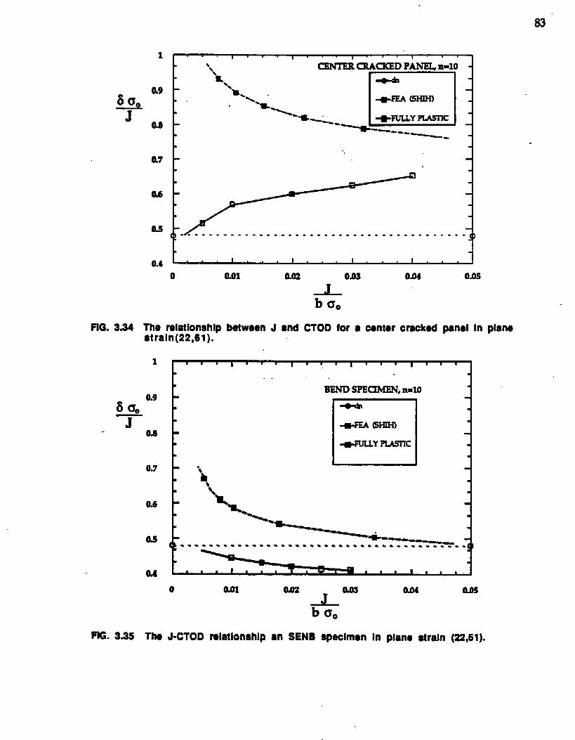
83”

1 I 1 1 I I 1

J

flG. 3.34

.-

OA

03 c~ ------- . . . . . . . . . . . . . . . . . . . . . . . . . 1~

0.4 1 I I I

o 041 mm 0,03 0.05J

b O.

The relatlonshlDbetweenJ ●nd CTOD for a center cracked nanel In Blanc. .straln(22,61). -

1

0.9

0.s

0.7

0.6

03

OA

[

. .

BENDSPE~, n=10 1

4-FM (5HIH)

~Y KAsnc

0

FIG. 3S5 TIM J-CTOD rslationshlp ●n SENB spaclmen In

OQ4

plane strain

0.0s

(22,61).

84

the El-c Power -arch Institute (EPRI) elastic-plastic fracture handbmk (82).The elastic-plastic finite element solutions were performed by Shih (22). In the caseof the center cracked panel (Fig. 3.34), the elastic-plastic J-CTOD relationship deviatessignificantly from the small scale yielding value. Note that the finite elementsolution and the fully plastic @imate tend to converge at high J valu=. lhe elastic-plastic J-CIOD relationship for the bend s@men is very close to d~ the fully plasticrelationship minddes with dn at moderately high J valus. Thus the small scale -yielding solution for the J-D relationship is fairly accurate for knd specimenswell into the pIastic range; the small scale yielding solution d- not apply to tensileldin~ =cept at very low J valu~.

The almve obsemations are consistent with the strss fields for bending.ti tension(l@ 3S4 and 3.2S). ‘Themade tip stres= in lxnding are close to the = solution athigh J vahms, but the center sacked panel cannot maintain sticient constraint withplastic deformation. A loss of constraint appears to be acmmpanied by a deviation ofthe J~OD relationship from Eq. [226]. Equation [3.271 implies that mn$~tit 1OS$is directly related to the J-CTOD relationship.

Neither J nor CTOD appears to have a clear advantage over the other parameter as ameasure of fracture toughness. When the assumptions of the HRR theory are .approximately vslid, the two parameters are uniquely related, and either csncharacterize sack tip conditions. When the HRR theory breaks down, neitherparameter characterizes crack tip conditions; both critical J and aitical CTOD value .depend on the configuration of the specimen or structure in such css~. Equation[3.m and Fig. 3.29 indicate that simultaneous measurement of both parameters may~ needed to characterize the critical conditions for fracture in large scale yielding.

3.8 CHARPY-FRACTURE TOUGHNESS RELATIONSHIPS

Fracture toughness testing is a relatively new phenomenon. In many industries, theCharpy V-notch (CVN) test is still the only accepted method for quantifying amaterial’s toughness. Most design codes for welded steel structures do not addr~sfracture mechanics methodology. Typically, these cod= spedfy a minimum CVNenergy for the base material and strict flaw tolerances for the welds. Both the CVNand flaw acceptance deria are usually arbitrary and often very consemative. Insome cm, however, fracture control procedure based on CVN toughness can benonmnsemative. For example, a large number of steeI bridg~ which were d~ignedwith such a procedure have sustained brittle fracture over the last 15 years (S3).

Since the Cha.rpy test did not become obsolete with the advent of fracture mechani=,there have been many attempts to correlate CVN toughness measurements withfracture mechanics parameters such as KIC. The problem with such correlations isthat the CVN testis very different from fracture mechan.i~ tests. The Charpy-en co~tfi a bl~t notch, while fracture toughna t~ts are performed on$peamens wdh sharp fatigue sacks. The Charpy -t is performed in impact loadin~

85

but most fracture toughn-s tests are prformed quasistatically. Another difihdtywith the Charpy testis that the spcirnen is small. Recall that fracture mechanics=ts must ~ performed on suf15aently large sped.rnens to guarante a singleparameter dtiption of uack tip”cond.itions. Wten the spedrnen is too small,toughnes is size dependerit; a small spedmen may indi=te ductile lxhavior, but alarge sped.men ~ted at the same temperature may be brittle

Most CVN-frachare correlations published to date are empirical. That is, the -investigators measured both CVN and KIc and then cun-fit the rcwdts to producea mathematical relationship between the two parameters. Because of the d.ifferenc~~ CVN and fracture mechanb ~ts, each of the empixical correlationsusually works well only for the material o@ally used to generate the correlation.None of these correlations mn h successfully applied to all st@ds (M).

Recently, some investigators have attempted to develop theoretical relationshipsbetween CVN and fracture toughness. These approadies ad- the differencesMw- the two typ of task.

3.8.1 Empirical Correlations

The various empirical correlations can produce widely differing estimates of KIcwhen applied to the same CVN data. Tbe approaches differ in three ways

1. The type of steel from which the correlation was generated

2 The way in which the data were fit;i.e., the form of &e equation “

3. lhe fracture khavior analyzed; e.g., transition region or upper shelf.

Some of the more common empirical correlations are summarized below.

Mandaret and Saru (85) applied a transition temperature approach to data for C-Mnsnd low alloy steels. They deilned the beghming of the transition at 28 J and 100 MPa

Kfor the CVN and KIC data, respectively. They correlated transition temperaturewith the following ~ression.

T ~IC 100) = 9 + L37T (~d B28]

where T is the temperature in ‘C. Assuming that the KIC and C’VN transition cww~had a similar shape, they estimated KIc at other temperatur~ from the followingrelationship:

KIC = 19~’

so

where K1c is in MPa ~ and *is in J. Note that one must apply thetemperature shift (Eq. [3.28]) when using the above ~ression.

Rolfe and Novak (86) developd the following correlations for upper shelf toughnssin steels:

m]”

where KICisin ksi~CVNisinft-lb, and~is inksi. Thegcd correlation withRolfe and Novak’s experimental data was attributed to upper shelf fracture not king

- as sensitive to notch acuity as cleavage An addition explanation is that upper shelftoughness data are not nearly as scattered as data in the transition region. Pisarski(84) pointed out that much of Rolfe and Novak’s data did not m=t the K1c sizerequirements snd were therefore not valid.

Rolfe and Barsom (87) developed the following correlation for the transition region.

KIC2—= 2 (cvN)3/2E [331j

.

where K1c is in psi ~, CVN is in ft-lb, snd E is in psi. The data displayed aconsiderable degree of scatter about the proposed correlation. The pm co@ation isprobably due to differ~ces in strsin rate and notch acuity. However, even a perfectcorrelation would not eliminate all data scatter in the transition region because it isan inherent feature of the material.

Barsom (80) attempted to reduce the scatter in CVN-fracture toughness correlationsby correcting for dynamic effects. He developed a two step correlation for thetransition region. Fust, he correlated CVN data with dynamic fracture toughness(Kid) tests. He then determined an empirid ~pera~e shift between KIc and K1ddata. Figure 3.31 shows some of the data for the latter comelation. Barsom fit K1dand CVN data for a nurnkr of stds to the following equatiox

KId2— =A(CVN)E @2]

where A is a constant The units on KE, CVN, and E are the same as in Eq. [3.31].For standard CVN specimens, A is approximately 5. This constant is approximately 4if the CVN specimen contains a fatigue preuack. The empirical temperature shiftbetween KIc and K1ddata is given by

87

where temperature is in ‘F and ~ is in ksi. Thus one mUSt first -timate a KIdvalue at a given temperature from Eq. [3.32], and then apply the tem~rature shift@. [333]) in ord~ to convert this -value into a KIC estimate.

lhere are several other ~-KIc correlations including those by Sailors and Corten(88), ~ey ~d Lo@on (89), and Ito et aL (90). Pisarski (84) reviewed a largenumkr of correlations and applied them to a range of experimental data. Hecurduded that most correlations work well for high strength steels but tend to be “consewative for low and medium slrength sW. Welhnan and Rol.fe (91) alsoapplied several published correlations to &ta for various steels; the empiricalcorrelations werked well on the lower shelf but were ~~sively conservative in thetmnsition region. The correlations failed to predict the rapid increase in toughness atthe onset of the ductil~brittle transition

Obsemations by P~ki (S4) and Wellman and Rolfe (91) imply that the empiricalCVN-KIC correlations apply only to linear elastic behavior, associated with the lowershelf or high strength steels; none work in the elastic-plastic regime.

DoIby (92) attempted to develop an elastic-plastic CVN-fracture toughness conflationfor weld metals, relating the O.lmm CTOD transition temperature to a correspondingCVN transition temperature. He concluded that acceptable correlations could befound only when the materials were stiaently delineated according to weldingprms, consumable=, etc. No universal CVN~OD mrrelation was found.

3.8.2 Theoretical CVN-Fracture Toughness Relationships

Some investigators have taken a more fundamental approach to CVN-fracturetoughness relationships. Norris et al. (93) developed an elastic-plastic, dynamic titeelement model of the Charpy -t and applied a local ductile failure uiterion to boththe Charpy specimen and a compact specimen to correlate upper shelf CVN energyWith JIC.

A somewhat similar approach by Anderson and Zapata (94) for the lowet shelf andtransition region used a statistical model developed by Anderson (43) to quantify theinherent miaostructural fracture properties of a given material. This information,in conjunction with Nonis’ finite element solution for the CVN specimen andsharp crack solutions by Shih and German (70), relate mauoscopic fractureProperti- of CVN and fracture toughn~s specimens. Since this model is statistical,it predicts not only average toughn~, but also any level of lower tmund.

15gure 3.36 (94) shows a sample comparison between experimental fracturetoughness and toughness predicted from CVN da~ The material was a 25 mm thickplate of ABS Grade EH36 steel. Experimental CTOD data are plotted with predictedmedian and 10% lower bound cunws. The agremmt between theory and_ent ~ me transition re@on is reasonably good, although the predictions areslightly consemative.

88

Anderson (95) also develo@ a theoretical relationship for the upper shelf that isdifferent from the Norris approach in attempting to characterize the slope of the Rcume rather than JIC. The R curve slope is ~timated by considering the tearingrwistance of a CVN spednen and relating it to initiation and propagation energy.The resulting ~r@on for the initial R cume slop is as fbllows

dJ4cvN~l .1”

)?lE = “W(2fp “~

where B and hre the thidcness and ligament length in the ~ s@men,_vely; f is the fraction of the Mal energy required for propagation; fi (= I-fP) is

Ethe initiation action; and n is the strain hardening exponent, as deiined in Eq. [2221.Predictions from Eq. [3.34] are compared in F5g. 3.37 with experimental data from a

- ofs= Pub~hed bY Gaw~ (%). For the pr~~o~ in Fig. 3.37, fp wasassumed to be 0.75 and n was assumed to equal 10. The agreement between theoryand qeriment is very god =cept for two data points at high CVN energy levels.

The theoretical CVN-fkacture toughn~s relationships for both the upper shelf andthe transition region should be investigated further. Although early resul~ areencouragin~ additional validation and refiement is needed to make suchapproach= practical.

One practical use of reliable correlations will be the evaluation of the structuralrekvance of existing CVN toughness uitena. If more quantitative measur~ of

~frachue toughness can h inferred from CVN vah.m, it will ~ possible to estimatecriticsl flaw ~ and sllowable deign stresses from the appropriate driving forcerelationships.

-.

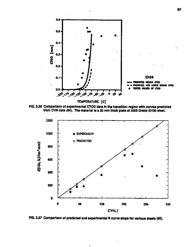
89

0.6

03

a4

%’&

03e

e02

al

090

●

☛

/

●

✃

●

●

✃

● ✘

● ●

I● 9#

● A’

Comparisonof experimentalCTODdata Inthetransitionregionwithoumespradktedfrom CVN data(64). ThematerialIs•35 mmthickplateof ABS Gmde EH36 steel.

0 PREDicrm

—

■

0 64 Y2s 192 256 320

m, J

Oompariaonof pradict@ and●xperimentalROUMelopefornrious stwls (95).

.

90

4. APPLICATION TO STRUCTURES

A sack will grow when the driving force for fracture =cds the mattial’sr=istance to fracture. Chapter 3 addr=sed the material rAstance side of theequation. This chapter focuses on the driving force.

4.1 HISTORICAL BACKGROUND

Fracture mechanb design anal- and driving fbrce equations have evolvedconsiderably over the last 30 years. The tit analyses were based on linear elastictheory and applied only to simple con@rations such as a center cracked panel.Now there are approach= which take account of most complications which arise inreal stmgtures, such as complex shapes, residual stress and large scale plastiaty.

4.1.1 Linear Elastic Fracture Mechanics (LEFM)

The LEFM approach to design can b summarized by r=taiing Eq. [2.6]:

[41]

where Y is a geometry correction factor, a is a characteristic stress, and a is acharacteristic crack dimension. The above relationship describes the driving force forfracture. The material fails when KI 2 KIG the material’s resistance to fracture.

Since Imin (5) and Williams (6) first applied the Wwtergaard (4} analysis to practicalproblems in 1957, most of the developments in LEFM have involved the generationof stiess intensi~ solutions (Y) for spcMc configurations. Most of the early analyseswere theoretical or experimental. Today, however, strss intensity solutions areusually determined from Wte element analysis.

Several handbdcs (8-10) contain compilations of stra intensity fact-. The mostrecent (and most complete) handbmk (10) contains K solutions for several hundredconjurations. It is now possible to find published K solutions that closely matchnearly any practical situation.

A number of variations to the LEFM approach attempt to comect for plastiaty, as.chsmssd in Chapter Z The Imin plastic zcme correction, where mack size is replacedby an effective mack length, extends LEFM to approximately 80% of the yield load (see13g. 29). The DugdaleBarenblati strip yield model (12,13) enables an effective K to becomputed up to limit load in nonhardening materials.

91

lhe development of J integral =t methods enables a linear elastic tiving forcerelationship to b applied in situations where it is not possible to measure valid KIcvalues in Ialmratory -ts. * dhcussd in Section 23.7, the J integral can oftencharacterize the crack tip cpnditioiis in a small spedmen, even though that spdnencontains a large plastic zone. A small spdmen and large structure loaded to thesame J value experience the same aa@ tip environment, as illustrated in Fig. 218.If the structure is ticiently large that the global bhavior is elastic, the crack tip .conditions can be &aracterized by either J or K Thus it is possible to estimate theKIc of the large stmcture fromthe JICofthe-specimem -

- .. [u]

Furthermore, one can use linear elastic driving force relationships (or LEFM with aplastic zone correction) to ~timate critical sack size or failure stress in the structure.

4.1.2 The CTOD Design CuWe

The CTOD concept was applied to structural st~ beghudng in the late 1960s. TheBritish Welding Research Institute (now known as The Welding Institute) and otherlaboratories performed CIOD tests on structural steels and welds. At that time therewas no way to apply th~ r~uhs to welded structures because ~D driving forceequations did not exist Burdekin and Stone (18) developed the CTOD equivalent ofthe strip yield model in 1966. Although their modeI provid~ a basis for a ~ODdriving force relationship, they were unable to modify the strip yield model toaccount for residual stressm and stress concentrations. (Th~ difikulties were laterovercome when a strip yield approach became the basis of the R6 d=ign method-)

In 1971, Burdekin and Dawes (97) deveIoped the CTOD design curve, a semi-empirical driving force relationship, that utilized fracture mechanics theory, whereavailable, and relied on empirical comelations and consemative assumptions forcircumstanc~ theory did not address. For linear elastic conditions, fracturemechanics theory was reasonably well developed, but the theoretical frameworkrequired to estimate the driving force under elastic-plastic and fully plasticconditions did not exist until the late 1970s Burdekin and Daw~ based their el.astic-plastic driving force relationship on an empirical correlation btween small scaleCT’OD tests and wide ten= sacked tension panels made from the same material.The wide plate spedmens were loaded to failure, and the failure strain and mack sizeof a given large scale spedmen were correlated with the uitiml CTOD in thecorresponding small wile t~t.

The correlation that resulted in the CIOD design mme is illustrated schemaiimlly inHg. 4.1. The uitical CTOD is nondimensio- by the half crack length, a, of thewide plate and is shown on the ordinate of the graph. The nondimensional CTOD isplotted against the failure strain in the wide plate, nomalized by the elastic yield

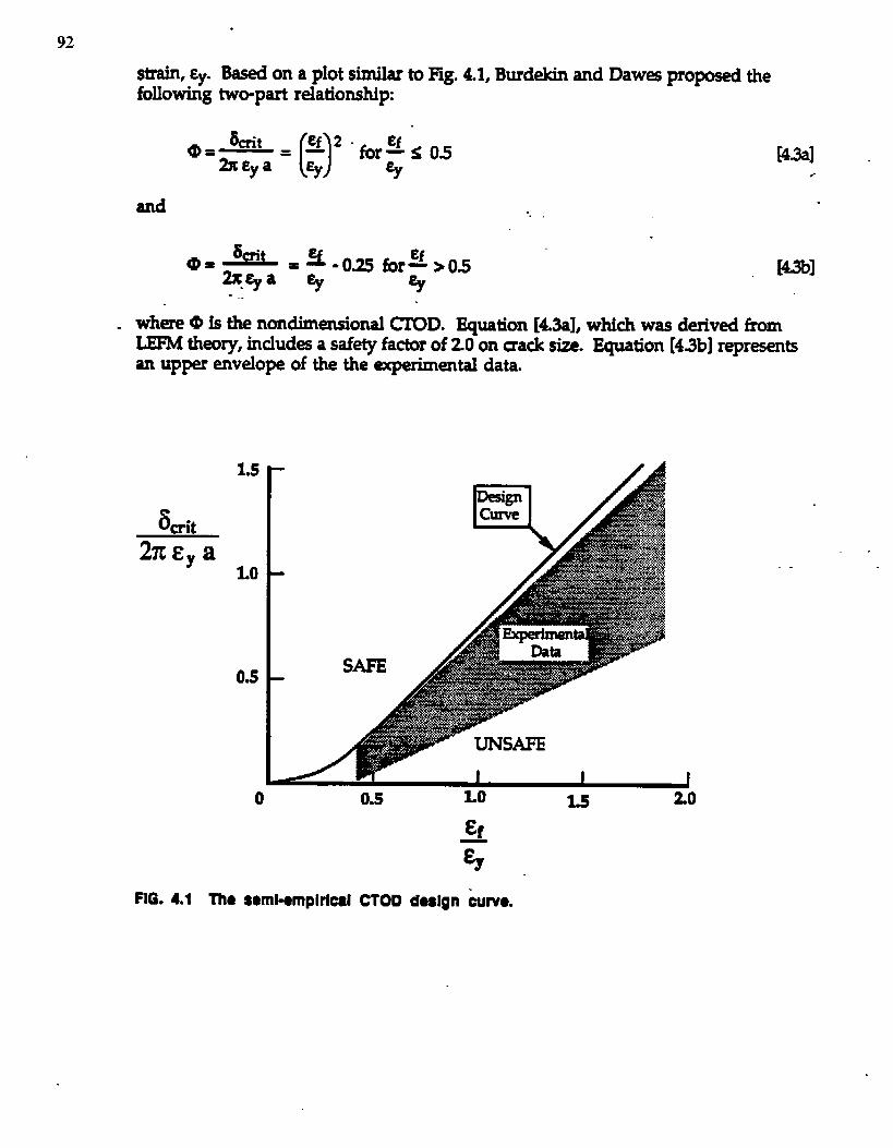
.92

strain, EY Based on a plot similar to Hg. 4.1, Burdekin and Dawa propsed thefollowing twepa.rt relationship

[43] .#

and -.

[m]

where 0 is the nondimensional C1’OD. Equation [43a], which was derived fromLEFM theory, includ= a safety factor of 20 on uack size. Equation [43b] representsan upper envelope of the the experimental data.

6crit

2X&y a

1.5

r

LO “

0.5 –

//

UNSAFE

I 1

o 0.5 Lo L5 20

&#

&,

FIG. 4,1 The soml+mplrical CTOD d~lgn &Jwo.

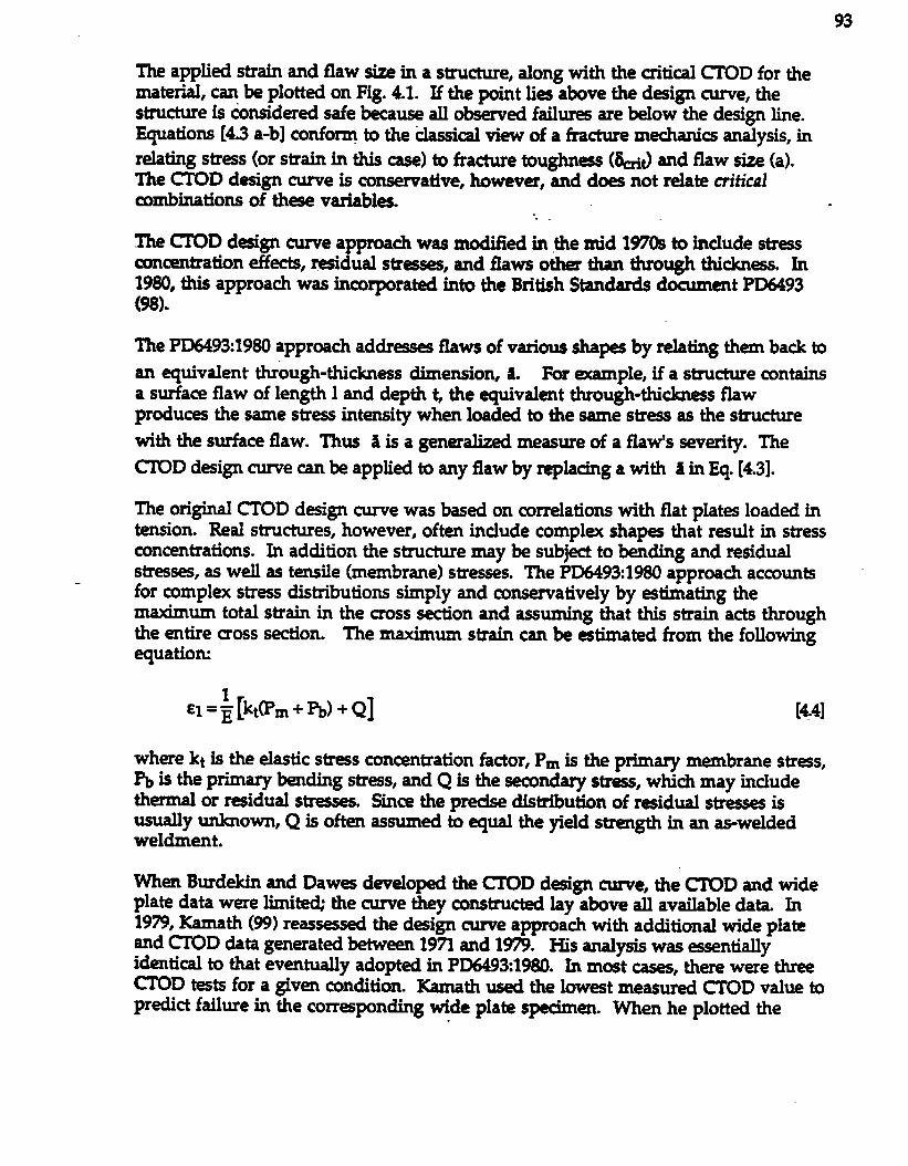
93

The applied strain and flaw size in a structure, along with the dical ~OD for thematerial, can be plotted on Fig. 4.1. If the point li~ almve the deign tune, thestructure is considered safe because all obsemed failur= are blow the design line.Equations [43 a-b] conform to the klassical view of a fracture mechani= analysis, inrelating stress (or strain in ~ case) to fracture toughn=s (~~ and flaw size (a).The CTOD design mime is consemative, however, and does not relate m“tical~tiiMtiOnS of th= variables.

The ~D d~gn -e approach was retied in the mid 1970s to include str~concentration effects, ~dual str~, snd flaws other than through thicknes. In1980, this approach was incorporated into the British Standards document PD6493(98).

?he PD6493:1980 approach addr~ flaws of various sha~ by relating them back to

an equivalent through-thickness dimension, ii. For ~ple, if a structure containsa surface flaw of length 1 and depth t, the equivalent throughthichess flaw

produces the same stress intensity when loaded to the same stress as the structure

with the surface flaw. Thus ~ is a generalized measure of a flaw’s severity. The

CTOD design -e can be applied to any flaw by replacing a with 5 in Eq. [4.3].

The original CTOD design curve was based on mrrelations with flat plates loaded intension. Real structures, however, often include compl~ shapes that result in stressconcentrations. In addition the structure may be subject to bending and residualstresses, as well as temile (membrane) stresses. The PD6493:1980 approach accountsfor complex stress distributions simply and mnsematively by estimating themaximum total strain in the moss section and assuming that this strain acts throughthe entire cross section. The maximum strsfn can be intimated from the followingequatiom

CI = ~ [kt(Pm + b) + Q] [44]

where kt is the elastic stress concentration factor, Pm is the primary membrane str=s,~ is the primary bending str-s, and Q is the secondary str~, which may includethermal or ~idual str-ses. Since the predse distribution of midual stress= isusually unhewn, Q is often assumed to equal the yield strengih in an ~weldedweldment.

When Burdekin and Dawes developed the CT’OD dtign cume, the CIOD and wideplate data were limite@ the came they constructed lay above all available data In1979, Kamath (99) remsed the d~ign -e approach with additional wide plateand CIOD data generated between 1971 and 1979. His analysis was ~sentidlyidmtical to that eventually adopted in PD64931$180. In most cases, there were ~~OD tests for a given condition. Kamath used the lowest measured CTOD value topredict failure in the corrqonding wide plate specimen. When he plotted the

results in the form of Fig. 4.1, a few data @nts lay Mow the design cume, indicatingEq. [4.3] was nonconsemative in these instances. The CTOD design cume, however,was conservative in most cases. Kamath estimated the average safety factor on macksize to& 1.9, although individual safety factors ranged from Ies than 1 to greaterthan 10. With this much scatter, the concept of a safety factor is of little value. Amuch more meaningful quantity is the confidence level. Kamath =timated that theCTOD design -e method corresponds to a 97-5% cotideme of s~v~. tit is, .the method in PD64931980 is co~ative approximately 97.5% of the time

4.1.3 The R-6 Failure Assessment Diagram

Structures made from materials with sufikient toughness may not be susceptible tobrittle fracture, but they can fail by plastic dlapse if they are overloaded. ThePD6493:1980 approach d= not expliatly addr~ plastic collapse, but impliady seeksto avoid collapse through an arduous flaw recategorization procedure.

The Centrsl Electricity Generating Board (CEGB) in Great Britain developed a designmethodology that takes account of fracture and collapse, as well as the interactionbetween these two failure mechanisms. The CEGB approach, known as the R-6method (100), is based on a modified strip yield model due to Heald et al. (101). TheR-6 method was fist published in 1976, with minor revisions in 1977 and 1980. (Athird, more radical revision published recently is dkussed in Section 4.2J

The R-6 method introduced the concept of a failure assessment diagram (FAD) todsuibe the int~action Mween fracture and collapse. The mo@fied strip yieldmodel and the failure assessment diagram that form the basis of the early versions ofWe R-6 procedure are desaibed below.

The effective stress intensity for a through-thickn~s sack in plane stress, accordingto the Burdekin and Stone (18) strip yield model, is given by

K?!H=cfYsG[$.sec(;$j’” [451

which is a r~tatement of Eq. [2.16]. As shown in Fig. 29, the above relationship isasymptotic to the yield strengtk This expr~ion can be m@fied for real structuresby replacing ~s with the d.lapse stress, cr~ for the structure. This would ensure thatthe strip yield mtiel predicts failure as the applied stress approack the collapsestress.For a structure loaded in tension, d.lapse occurs when the stress on the netcross eon reach= the flow stress of the material. Thus ~Cdepends on the tensilepropd~ of the material and the flaw size relative to the total cross section of thestructure. The n~ step in deriving a failure assessment diagram from the strip yieldmtiel entails dividing the effective stress intensity by the linear elastic K

lhis modification not only- qre the driving force in a dimertsionl=s form butalso eliminates the square root term that contains the the half mack length of thethrough crack Thus Eq. [4.6] is more general, in that it applies to all configurations,and not just a through-thickn~s sack in an infupte plate. This is analogous to the -PDM93 approa~ wlwe the driving force relationship was gengralfzed by detining

an equivalent through thickness flaw, ~ & a W step, we can define the stressratio, ~, and the K ~tiO,K,,asfdows

and

s,:=-

WI

The failure assessment diagram is then obtained by inserim“ g the above definitionsinto Eq. [43] and taking the redprmak

‘r=+h=bl]-’”Equation [4.9] is plotted in 13g. 4.2. The cu.me reprsen~ the locus of predicted failure@nts. Fracture is predicted when ~ff = KIC. If the tou~s is very large, thesixucture fails by collapse when S, = 1.0. A brittle material will fail when Kr = 1.0. Inintermediate ~, collapse and fracture interact, and both Kr and S, are less than 1.0at failure. AU points inside of the FAD are considered safe; points outside of the~agram are unsafe.

In order to -S the signiikance of a particular flaw in a structure, one mustdetermine the applied value of Kr and $ and plot the point on Eg. 4Z Thes-intensity ratio for the structure is givm by

K1K, (Struchue) = ~ IuO]

.

96

12

1

Kr

0,s

u

004

02

0

0 02 0.4 0.6 Oa 1 u

s,

FIG. 42 The R-6 faiiuro saseasment diagram baaed on the strip yitid modei.

The applied stra ratio can be defined as the ratio of the applied str~s to the collapsestress. Alternatively, the applied ~ can be defined in terms of axial forces ormoments. If the applied conditions in the structure place it inside of the FAD, thestructure is safe.

The 1980 R-6 document (100) offers practical advise on how to apply the strip yieldFAD to real s~ctur~. For example, it recommends that sfress~ be taken intoaccount through a semndaiy stress intensity. Ihe total stress intensity is obtained byadding the primary and secondary components:

KI = KIP + KIS [411]

Only the primary ~ are used to compute ~ kause secondary str=ses, bydefinition, do not contribute to collapse. Note that K1 is the LEFM s-s intensity; itdoes not include a plastic zone mrrection Plasticity effects are taken into accountthrough the formulation of the failure assessment diagram (Eq. [4.9]).

The R+ procedure reco~ends that the fracture toughness input be obtainedthrough testing the material according to ~ E399 or the equivalent British

97

Standard. When it is not possible to obtain a valid KIC value qerimentally, onecan measure JIC in the material and convert this toughna to an equivalent KIC bymeans of Eq. [4.2].

4.1.4 Tho EPRI J Estimation Procedure

The R+ failure as~sment diagram is based on a strip yield model. Since it assumes.elastic-perfectly plastic material behavior, it is co~ative when applied to strainhardening materials.

In 1976, Shih aid Hutchi.nson (102) proposed a more”advanced methodology for~@ng W fracture driving force which takes account of strain hardening. Theiri@@ach, developed further and validated at the General Electric Corporation inSchenectady, New York in the late 1970s and early 1980s, was published as anengineering handhk by the Electric Power Researh Institute (EPRI) in 1981 (82).

The EPRI procedure provides a means for computing the applied J integral underelastic-plastic and fully plastic conditions. The elastic and plastic components of J arecomputed separately and added to obtain the total ~

Jtot = JeI + Jpl [4.12]

The ektic J is equal to G, the en~gy release rate. The EPRI handbook states that J~should inchde a modifmd first order plastic zone correction, but this correctiontypically affects the total J by no more than 5% (102). Since this plastic zonecorrection has no theoretical basis snd severely complicat~ the analysis, manyengineers omit the conection on J~.

For the fully plastic J, Shih and Hutchinson assumed a power law stress-plastic straincume (Eq. [2.22]). The nonlinear elastic assumption on which J integral theory isbased implies proportional loading local stresses must incresse in proportion toremotely applied forc~ and moments. Hence the HRR singularity (Eqs. [2.23] and

[Z24]) implies that J 1is proportional to ~+1, where P is a remote load. Shih andHutchinson invok J proportional loading and dimensional analysis to show that JPIcan k ~ressed in the following form

[413]

where POis a refemme load and hl is a dimensionless constant that depends on theconfiguration and the strain hardening expnent. The terms a, ~, and aO arematerial flow properties, as defined in Eq. [222], and b is the untracked ligamentkngth in the structure or test specimen. Shih and Hut-n ~ derivedexpressions for the plastic mack mouth opening displacement, VP, and the plasticload line displacement, Ap:

98

Pn

()VP= a 6 a hz(a/W, n) ~

Pn

()Ap= a q a h3(a/W, n) ~.

o -

where hz and ha are dhrmsionless constants for””thecorrespondingmeasurements. The EPRIhandbook lists hl, hz and hs valb for;

[414]

[415]

displacementVdety of

configurations and strain hardening rates. These cmstan~ were dete- bymte element+analysis. .

Figure 43 is a plot of applied J in a cmter sacked panel with a/W = 0.5 and n = 7.Note that the elastic term dominates at low loads and the plastic term dominates athigh loads.

The elastic-plastic driving force ~timated from the EPRI procedure can also beqp=sed in terms of a failure aswsment diagram, an idea fist proposed by Bloom(103) and Shih et al (104). The J ratio and stress ration are defined as follows.

G‘r= G+Jp~

and

[416a]

[4.16b]

The equivalent Kr is qyal to the square rmt of Jn

Rgure 4.4shows the applied J for center cracked panels with a/W= 0.5 and 0.75,plo=d in terms of failure ass~sment diagrams. The R+ diagram is included forcomparison. Note that the shape of the FAD changes when strain hardening is takeninto account. The R4 diagram is consenative in this case because it assumescollapw will occur wha the net section str=w equal cd a panel made from a strainhardening material could withstand somewhat greater stresses. Figure 4.4 alsoillustrat~ that failure assessmmt diagrams derived from the EPRI procedure aregeometry depdent, while the R+ diagram is geometry independent. This makesfracture anal~ with the ~ approach more complicated, Iwcause a different FADmust be generated for each con@.rafion analyzed

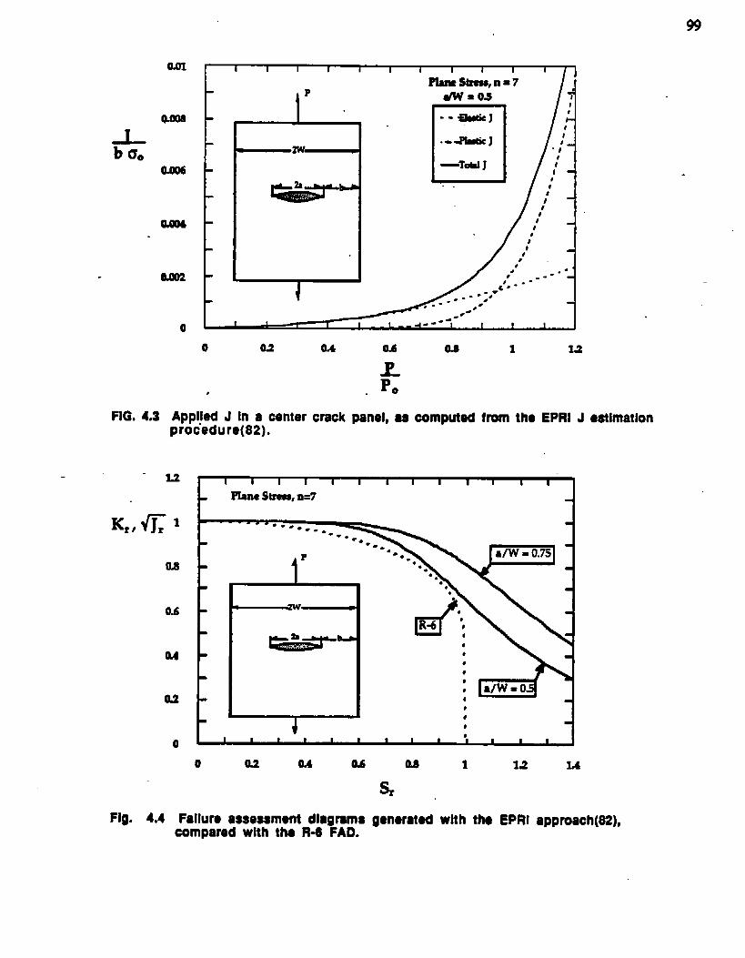
99

0.o1 1 i I I r I I I I I 1 i I i

.

Pi8mS&CU, n=7 ‘,P M=os 14I

o

I

.

FIG. 4.3

0 02 a4 0.s 1 la

;. P.,

Applled J In a center crack panel, ●s oomputed from tho EPRI J ●atlmationprocedure.

u P1 I I 1 I I I i i I I I I

PlanestrHS,n=7

0.s

0.6

u

02

Fig. 4,4

H

0. 1

o u 0.4 04

Failure assessment diagramsoompared with tho R-8 FAD.

me 1 u L4

s

gensrated with tho EPRI approach,

100

Ssctlon 4.1.5 Recent Advances in Elastic=PIastlc Analysls

lhe ~OD d~ign cume was the first elastic-plastic fracture analysis, developed whenelasti~plastic fracture mec@n.i= was in its infanq. The th=retical work of Rice andothers had not yet filtered down to eng%eers. Burdekin and Daw= had to rely onempirical correlations and consenativi assumptions to develop a comprehensiveelastic-plastic fracture dsign approa~. The CEGB R-6 method, which wasdeveloped a few years lat~, was based on an ov-pl.ifd theory of crack tip -plastidty. The work of Shi.h and Hutchinson in 1976 was the fist sound theoreticalframework for analyzing nonlinear fracture in structur~. Their work tie thebasis of the EPRI approach, published in 1981. .

One problem with the EPRI procedure has ~ that it can only ~ applied torelatively simple configurations. In addition, this method givs no guidance on thetreatment of sem-ndary stresses. Recent advancs have improved the EPRI approachsomewhati additional configurations have been analyzed (1(5107) since the originalEPRI report was published, and Bloom (108) has proposed a failure assessmentdiagram approach that utilizes EPRI J solutions and a secondary stress analysissimilar to that of the R6 procedure.

Both the R+ method and PD6493 have been revised recently to incorporate some ofthe thmretical work upon which the EPRI handbmk is based. Ih~ new documentscombine the flexibility and wide applimbility of previous versions with more sound oelastic-plastic driving force analyses.

Recent work by Ainsworth (109) allowed the two British procedures to be updated -while retaining their flexibility. Ainsworth’s main contribution was to simplify theEPRI approach without sad.fming accuracy. The basis of A.insworth’s reference str~smodel is described below.

4.2 THE REFERENCE STRESS APPROACH

The EPRI equation for fully plastic J, Eq. [4.13], assure= that the material’s stress-plastic strain cuwe follows a simple pwer law. Many materials, howev=, haveflow khavior that deviates mnsiderably from a pwer law. For example, most lowcarlmn std exhibit a plateau in the flow -e immediately after yielding.Applying Eq. [4.13] to such a material, rmd~ in si@cant errors. Ainsworth (109)modii5ed Eq. [4.13] to reflect more closely the flow Mmvior of real ma-. Hedefined a refererw s-s as follows:

He further defined the reference strain as the total axisl strain when the material isloaded to a uniaxial str~s of 6*. Substituting these de~tions into Eq. [4.13] gives

101

[4.18]

lb materials that obey a potwr law, Eq. [4.18] agr~ precisely with Eq. [4.13], but Eq.[418] is more general, in that it is applicable to all types of dr~strain behavior.

Equation [4.18] still contains hl, the geometry factor which depends on the power law-hardening expnent m Ainsworth proped redefining POfor a given configurationto produce another constant, hi’, that is insensitive to n. He noticed, however, thateven without the modification of PO,hl was relatively insensitive ton except at highn valu- (low hardening mataials). Ainsworth was primmily interested indeveloping a &iving force procedure for high hardening materials such as austmiticstainbs steels. The strip yield failure assessment diagram was considered suitablefor low hardening materials. He proposed the following approximation

hi(n)s hi(l) [419]

where hl (n) is the geometry constant for a material with a strain hardening exponentof n and hi(l) is the corr~ponding constant for a linear material. By substitutinghi(l) into Eq. [4.18] (or [4.19]), Ainsworth was able to relate the plastic J to the linearelastic s~ess intensity factor:

[420]

where L = 0.7S for plane strain and y = 1.0 for plane stress.

Ainsworth’s work has important rauMcations. When applying the EPRI approa~one must obtain a str~ intensity solution to compute the elastic J, and a separatesolution for hl in order to compute the plastic tm. The hl constant is a plasticgeomq correction factor. However, Eq. [4.20] makes it possible to estimate JP1froman elastic geometry correction factor. The original EPRI handbmk (82) andsubsequent additions (105-107) contain hl solutions for a relatively small n~ber ofconfigurations; but there are several hundred str~s intensity solutions in handbooksand the literature. llm.s Eq. [420] is not only simpler than Eq. [4.13], but also morewidely applicable. The relative accura~ of Ainsworth’s sifnpli.fmd equation isexsmined in Section 4.4.

Ainsworth made additional shnplil%ations and modifications to the reference stressmodel in order to ~ress it in terms of a failure as~sment diagram. This FAD hasbeen incorporated ihto a revision of the R4 procedure. The new document alsocontains more accurate procedure for analyzing seconday stress=. The revised R-6approach still permits application of the strip yield FAD to low hardening materials.

102

lhe reference stres FAD has also been included in the revised PD6493 procedure, to~ published in late 1989 or early 1990. This approach, demibed lAow, is broadlysimilar to the revised R4 method.

4.3 THE THREE-TIER APPROACH (REVISED PD6493)

The CTOD dtign cu.me, which is the basis of PD64931960, suffers from a number of”shortrmnings. For ~ple, the driving force equation is mostly empirhd and has avariable level of mnsenatisrn. In addition, this approach d= not ~liatly-der failure by plastic dlapse. Improved driving force equations becameavailable with the R+ and EPRI pnxechares, but the CIOD design curve had alreadyben widely accepted by the welding fabrication industry in the United Kingdom andelsewhere. Many engineers are reluctant to discard PD64931930. Structuresdesigned according to the original PD6493 method might have to be re-analyzed withthe new procedure if the CTOD design cume were rendered obsolete. An additionalproblem with improving the prwedure the tendenq for the more accurate elastic-plastic fracture snal~ to be more complex and require more training.

The conflicting goals of improving PD6493 and msintairdng continuity with the pasthave k largely satisfied by a three-tier approach. his idea was originallysuggested by Anderson et al. (110). The three tier philosophy assesses fractureproblems at a level of compkity and accu.ra~ appropriate for the situatiom Allthree levels of PD 6493 are expressed as failure assessment diagrams. bvel 1 isconsistent with the CTOD design tune approach; Level 2 utilizes a strip yield modeland is similar to the 1980 version of the R+ method; Level 3 is based on thereference stress model and is nearly identical to the revised R-6 procedure. Unlikethe R4 approa~, however, the revised PD 6493 permits assessments based on CTODasweUas Jand K

Although the new PD6493 procedure has not been published, a number of recenttick (111, 112) describe its salient features. Information in the followingsubsections is based on these articles.

4.3.1 Level 1

Level I is consistent with the CI’OD deign cume in the 1980 version of PD6493. Theresin differenaM are that the equations are expressed h-i terms of a failure _smentdia&ram, and an explicit COkpse tiySiS is included. Levd 1, WhiChis~ative, is intended as a screening tool.

If KIc data are used (or equivaknt K valu~ from J data), the K ratio is dei%wd by Eq.

[4.10]. Mr CIOD data, K, is replaced by ~~, defined as

103

[al]

where al is the appliedCusve

~D obtained from a modified form of the ~OD d=ign

K*2 -.&*- for q/qs 50.5

WEwad

where 61/E = q, the maximum membrane sirain defined in Eq. [4.3]. Recall that&l

(d thUS @ ta.k$ tidual stresss, banding str~, and stress concentii~ons intoaccount by assuming that the maximum value of the total stress acts uniformlythrough the cross section. Unlike Eq. [4.2a], the above expression does not include asafety factor of two on mack size. In the revised approach, this safety factor is

included in the formulation of the FAD, wMA is a horizontal line at ~h = l/fi forcl/qs S 0.5. The Level 1 failure assessment diagram is illustrated in Fig. 4.5(111,112). For higher stress levels, the assessment line is defuwd from the empiricalportion of the CTOD design -e .

“=s(32(:-0=)‘m”l’m’O’ [4z2b]

The influence of Equation [4.22b] on the FAD is illustrated in Fig. 4.5. The revisedCTOD design curve contains a co~ative collapse check in the form of amaximum stress ratio, ~. For Level 1, ~ is defined as

%=s [alaflow

where an is the effective primary net section stress and Gflowis the flow stress,

defined as (m + @/2 or 1.2 %, whidwm is less. & Hg. 4.5 indicat=, the Level 1approach is r~tricted to 04 Sr because Eq. [4.22] can be nonconsenative near limitload (110).

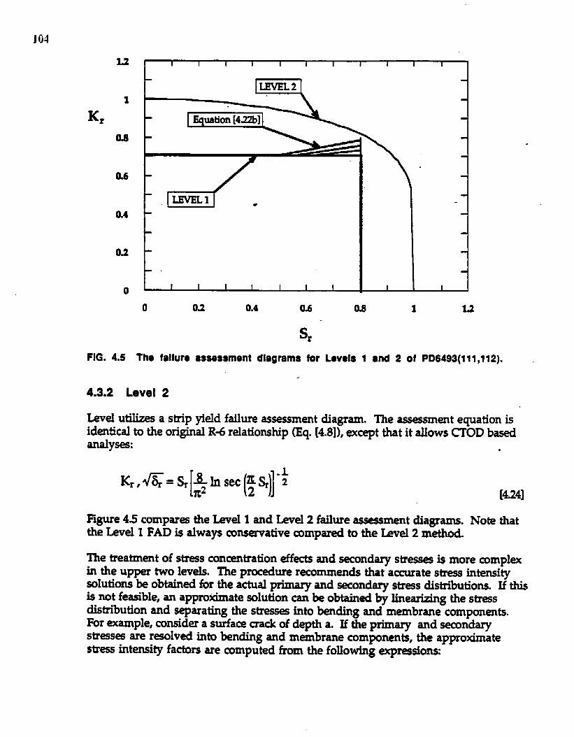
104u

1

K,

04

a6

a4

u

o

I I I I i i I I I i I

LEvELl *

I I I I I I I I I

o 02 0.4 0.6 0,6 1

s,

FIG. 4.5 Th@ failure assessment diagrams for Lev81s 1 ●nd 2 of

.

4.3.2 Level 2

12

PD6493(111,112).

Level utilizes a strip yield failure assessment diagram. The assessment equation isidentical to the original R+ relationship @q, [4.8]), except that it allows CTOD basedanalyse:

●

“’K=S’[9S’C(HI-; [424]

Hgure 4.5 compare the Mel 1 and Level 2 failure assessment diagrams. Note thatthe Level 1 FAD is always consewative compared to the bvel 2 method.

The treatment of str~s cmmntration effects and secondary str~ is more complexin the upper two levels. The prmedure recommends that accurate stress intensitysolutions be obtained for the actual primary and secondary str~s distributions. If thisis not feasible, an approximate solution can be obtained by Iinearizin g the s-sdistribution and separating the str- into bending and membrane components.For ~ple, consider a surface mack of depth a. If the primary and semndarystr=ses are r~olved into lwnding and membrane components, the approximatestress intensity factors are computed from the following expr~siorw

105

Klp F=+J’m+MbPd [-1

where $ isthe flaw sha~ parameter, Pm and ~ are the primary membrane andkuiing str-a, Qm and Qb are the secondary siresses, and Mm and Mb are constantsobtained from the Newman and Raju stress intensity solutions (113). If, as in many-, the actual distribution of ~ndary str~~ is unknown, one should assumethat Q acts uniformly auoss the sectiom The document recomm endsthat Qbe

- assumed to equal the material’s yield strength in the case of as-welded compxientsFor thoroughly str~ relieved weldmmts, the estimate of Q can & reduced to 30% ofyield parallel to the weld and 15% of yield transverse to the weld.

The total K1 is the sum of the primary and secondary contributions. For assessmentsbased on ~OD, 51 is estimated from K1 by assuming plane stress conditions

[426]

There is a plastic int~action between primary and secondary interaction that must betaken into account in Level 2 This is achieved with the comection factor, p, based onthe work of A.insworth (114). The applied toughness ratios for the structhre aregiVen by

K1

“=G+P

and

[427q

[al

The value of the p factor decrm as the limit load is approached because secondarystmses are relieved by plastic sh’ain. When a structure is prmf -ted, a portion ofthe residual stress are relieved The revised PD6493 approach lets the userincorporate the benefits of prmf testing into the analysis.

106

The stms ratio, ~, is defined as the ratio of the effective net section stress to the flows-, as in Level 1. When the point defined by Eqs [4.23], [4.27J and [4.281 falls insideof the Level 2 assessment line (Eq. [4.24]), the structure is considered safe.

4.3.3 Level 3

The LeveI 3 failure as-sxnent diagram is based on Ainsworth’s reference str~s .approach (109). The FAD is related to the mate@d’s str~s-stmin behavio~

The above quantity is plotted against the load ratio, ~, de.fmed as

[430]

Note that ,the reference stress and the effective net section str~s are equivalent.Since the load ratio is defined in terms of the yield strength rather than the flowstr~, Lr can be greater than L The load ratio cannot exceed 6fIow/oys, where Cflowis ddined as the average between yield and tensile strengths. For Level 3, thealternate definition of flow stress (aHOW= 1.2 ays ) does not apply. For Lr > oflOW/aYS,~=o.

If the stress-strain cume for the material is not available, such as would be the casewhen analyzing a flaw in the heat affected zone, the following FAD equation can beapplied at Level 3

Kr, {~ = (I - 0.14 L#)[0.3 + 0.7exp (~.ti ~6)] [431]

This expression also has a cut-off at ~ = OflOw/ayS. Equation [4.31] was adopted fromthe latest version of the R-6 procedure (115). This alternate FAD requires ahowledge of only the yield and tensile strengths of the material, but thisrelationship can be ~-sively consemative (112). For many materials, Eq. [4.31] ismore con.semative than the Level 2 FAD. Figure 4.6 is a plot of Eq. [431]. Note that “the upper cutmff on ~ depends on the hardening characteristi~ of the material. Ifthe material has a yield plateau, the revised PD6493 recommends that Eq. [4.31] bemtrictedto~sl.

TheLevel3 analysisof Kr (or ~~ ) for the structure is identical to the Level 2_ures (Eqs. [4.26] - [4.28)), but Level 3 i.nclud- guidelines for ductile instabilityand tearing analysis. This type of analysis is dbbed in Section 4.5.

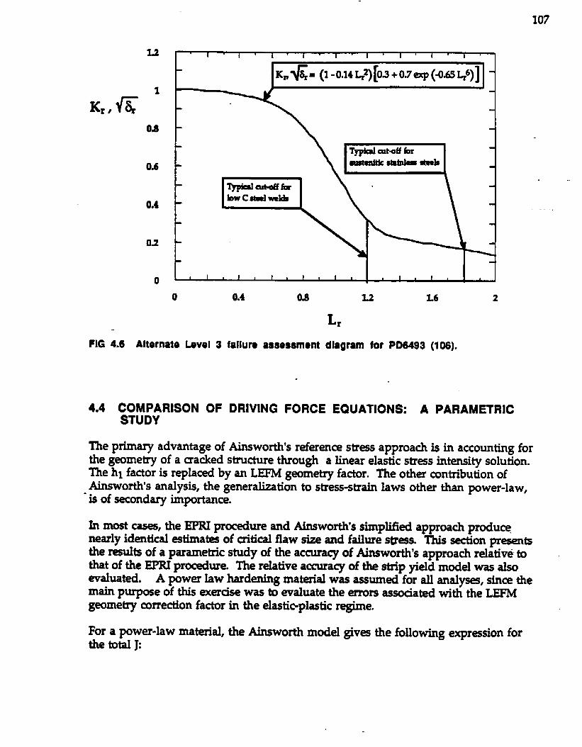
107

0.6

0.4

0

1 I I I 1 I I I

Km~= (I -0.14~2)[03 +0.7exp (4= Q)]

8W&nitk$!8inlmti

bwctiti

1 I 1 1 I I I I I

o 0.4 0,s u L6 2

L,

FIG 4.6 Alternate Lsvel 3 faiiuro assessment diagram for PD6493 (106).

4.4 COMPARISON OF DRIVING FORCE EQUATIONS: A PARAMETRICSTUDY

The primaxy advantage of Ainsworth’s reference stms approach is in accounting forthe geometry of a sacked structure through a linear ela;tic stress intensity solu~on.The hl factor is replaced by an LEFM geometry factor. The other contribution ofAinsworth’s analysis, the generalization to stress-strain laws other than power-law,

“is of secondary importance

In most cas=, the EPRI praedure and Ainsworth’s simpl.ifwd approach producenearly identical estimates of critical flaw size and failure sb~s. This section presmtsthe results of a parametric study of the accuraq of Ainsworth’s approach relativ# tothat of the EPRI procedure The relative accuraq of the strip yield model was alsoevaluated. A pwer law hardening material was assumed for all ana.1~, since themain purpose of this exerase was to evaluate the errors astiated with the LEFMgeometry correction factor in the elastieplastic regime.

For a power-law material, the Afnsworth model givm the following expression forthetotal~

108

Since stressintensity is proportional to load, this

J= c@ + C2P+1

[432]

relationship has the form

The fist term domina~ under Iinesr elastic conditions; the second term dominatesunder fully plastic conditions. The EPRI approach (Eqs. [4.12] and [4.14]) has the sameform The only difference between the EPRI equation and Eq. [4.32] is the value ofthe constant C~ the equations a- precisely in the linear elastic range. Thus any . .discrepandes btween the two approdw are obsemed only when the plastic term issignificant.

When the plastic term dominate, J is very sensitive to the applied load. A smallemor in the Stimate of P results in a large error in the Stimate of J, but thissensitivity bean advantage when predicting failure. Since J is very sensitive to load,P is very insensitive to J, implying that the fi$lure load in the plastic range isinsensitive to the fracture toughness; i.e. the critical J. In the fully plastic range, .failure is essentially collapse controlled rather than fracture controlled, as seendearly in the failure assessment diagram in Fig. 4.2. As the str=s ratio approach=unity, the diagram becom~ nearly vertical, in-dcating that the failure sti-~s isindependent of the toughness ratio. At these high stress ratios, the failure stress

governed by the material’s flow properties rather than its fracture toughness.

The predicted failure stress in the fully plastic rarige is slso insensitive to thedifferences between the EPRI approach and the Ainsworth model. The latter

is

approach assumes that the georn-etry factor, hl (n), is equal to the linear elastic value,hi(l). Errors in J that result from applying Eq, [4.32] are proportional to the ratiohi(n)/hi(l), plotted against n in Fig. 4.7 for a center sacked panel in plane strain witha/W = 0.75. Note that the hl ratio in this configuration is sensitive to the hardeningacponent. Thus Eq. [4.32] leads to sign.ihnt errors in J, particularly at high n vahm.However, when the hl ratio is rakd to the power 1/tn+lJ, it is insensitive to n. Thislatter ratio is indicative of the differences in the predicted failure str~s between theAinsworth and EPRI approaches.

A d=ign engin- often wish- to use a fracture mechani~ analysis to -timate thecritical flaw size at a given applied s-s. To determine the sensitivity of uitb.1flaw size ~timat~ to the driving force equation, a serk of calculations wereperformed with the EPRI, Ainsworth, and strip yield mdels on center mackedpanels and edge sacked bend spdnwns. Hardening exponen~ of 5,10 and 20 wereassumed. Only plane strain conditions were considered.

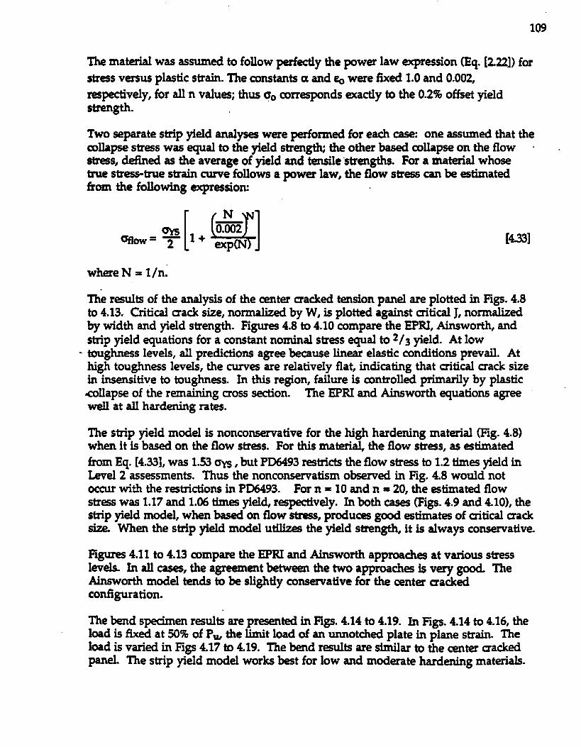
109

‘I’hematerial was assumed to follow perktly the ~wer law qression (Eq. IZnl) fm

stms versus plastic strsin. The constants u and ~ were fixed 1.0 and 0.002,=Pectively, for all n values; thus go corr~onds exactly to the 0.2% offset yieldstrength.

Two wparate strip yield anal- were #ormed for each case one assumed that thecollapse str-s was equal to the yield strength; the other based collapse on the flow - .-s, defined as the average of yield and tensile “strengths. For a material whosetrue stress-tie strain cume follows a pver law, the flow stress can be -tirnatedfrmn the following expresaiom

[ (-2]N

maflm=y 1+@N) [-1

where N = l/n~

The rsults of the analysis of the center macked tension panel are plotted in F@ 4.8to 4.13. Critical crack size, normalized by W, is plotted agsinst criticsl J, normalizedby width and yield strength. Figures 4.8 to 4.10 compare the EPRI, Ainsworth, sndstrip yield equations for a constant nominal str-s equal to z/3 yield. At low

- toughness levels, all predictions agr- because linear elastic conditions prevail. Athigh toughness levels, the cumes are relatively flat, indicating that critical crack sizein *sitive to toughn=s. In this region, failure is controlled primarily by plastic

<oIlapse of the remaining cross section. The EPRI and Ainsworth equations agreewell at all hardening rates.

The strip yield model is nonco~ative for the high hardening material (Fig. 4.8)when it is based on the flow str-s. For this material, the flow stress, as @imatedfrom Eq. [4.33], was 1.S3 CrYS,but PD6493 rstricts the flow str= to 1.2 ties yield ~Level 2 assessments. Thus the nonconsematism obsmmd in Hg. 4.8 would notoccur with the reslxktions in PD6493. For n = 10 and n = 20, the estimated flowstr- was 1.17 and 1.06 times yield, r~pctively. In both cases (F@. 4.9 and 4.10), thestrip yield model, when based on flow m, prdu~ gmd 4mat~ of critical cracksize When the strip yield mdel U- the yield strength, it is always consemative.

FI~ 4.11 to 4.13 compare the EPRI and Ainsworth approach= at various stresslevels. In all cases, the agreement between the two approaches is very good TheAin.sworth model tends to & slightly consemative for the =nter sackedcor@uration.

The bend specimen results are presented in Figs. 4.14 to 4.19. In Figs. 4.14 to 4.16, theload is fied at 50% of PW the limit load of an unnotdied plate in plane straiIL Theload is varied in Figs 4.17 to 4.19. The bend ~ts are similar to the center crackedpanel- The strip yield model works bst for low and moderate hardening materials.

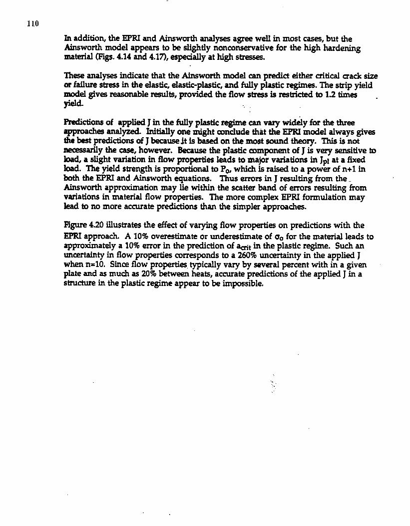
11,0

In addition, the EPRI and Ainsworth analyses agr~ well in most cm, but theAinsworth model appears to be slightly nonmnsawative for the high hardeningmaterial (Figs. 4.14 and 4.17), es@aUy at high str~.

Ih- anaIyses indicate that the Ainsworth model can predict either critical ~ack sizeor failure strms in the elastic, elastic-plastic, and fully plastic reginw. The strip yieldmcdel giv= reasonable tits, provided the flow str=s is =H- tO 1.2 tie .yield -.

Rdktions of applied J in the folly plastic regime can vary wid~y for the thrwe~~ ~~. ~~y OIWtight conclude that the EPRI model always givetiWtprddom tiJhujth Monb~st~d~~. Thisisnot~arily the case, however. Because the plastic compwnt of J is very sensitive toload, a slight variation in flow proprties leads to major variations in Jpl at a fied&ad. The yield strength is proportional to PO,which is raised to a power of n+l inImth the EPRI and Ainsworth equations. Thus errors in J resulting from the.

Ainsworth approximation may lie within the scatter band of emors ~uhing fromvariations in material flow properties. The more complex EPRI formulation maylead to no more accurate predictions than the simpler approach=.

Figure 4.20 illustrates the effect of varying flow propertk on predictions with theEPRI approach. A 10% overestimate or underestimate of UOfor the material leads toapproximately a 10% error in the prediction of -tin the plastic regime. Such anunmrtainty in flow properties corresponds to a 260% uncertainty in the applied Jwhen n=10. Since flow properties. typically vary by several percent with in a givenplate and as much as 20% between heats, accurate predictions of the applied J in astructure in the plastic regime appear to be impossible.

‘,,

. .

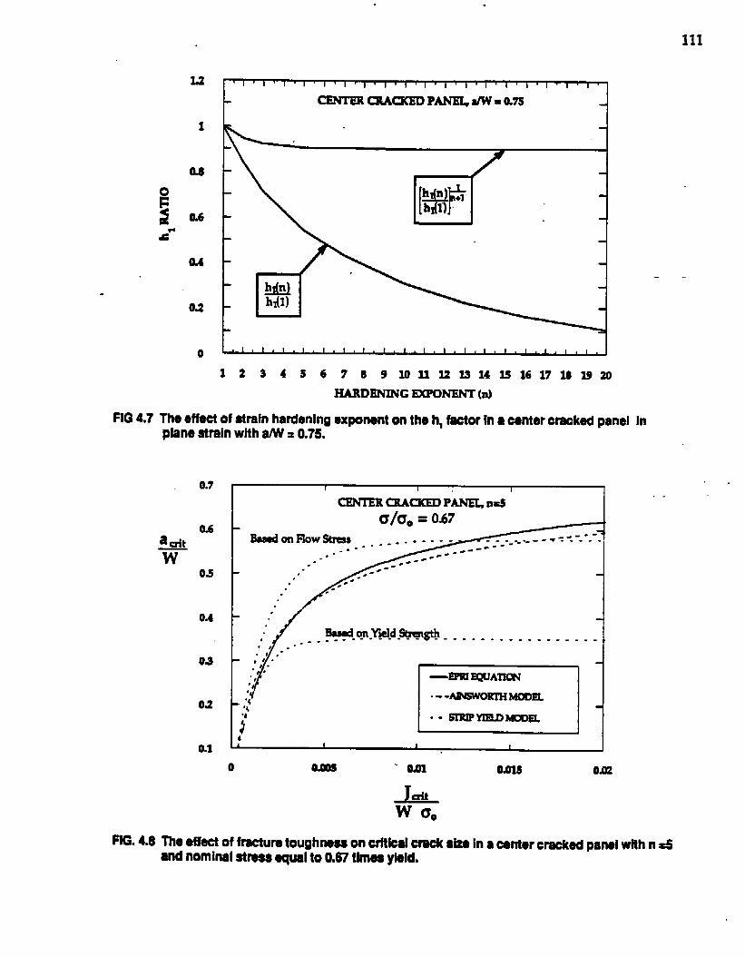
111

1

as

eA

.

Oa

o

I I I I I I I I I I I 1 I i I I I I

cENTEacmcKED Pm&iw=a7s

1. I.I. I I I I I 1 I 1 1 I I I I I I I

-.

12345678910 II 2215141516 W1319ZI

HARDENINGHNENT (al

FIG4.7Tho effect of strain hardeningexponenton the h, factor in ● center cracked panei InpianostrainwithW= 0.75.

0.7. .

I 1 I I I

CENER WCKED PANELn=3 I. .

O/aa= 0A7

B&w$mFh3wstm$ . . -----.-- ”--. ..-.-

.“...

0.4

03

1

. / I

‘/ 1ti.qn.Yjdd.*@ ................., .+----

j’ I .- smPYlmDMmEL

0.1 L I 1 I

o “ OAI Oms Om

Js!kw 00

FIG.4.8 The effectof fmcturatoughnesson criticalcracksize in ● centercrockedpaneiwithn =8andnominaiatreasequaito 0.87 times yieid.

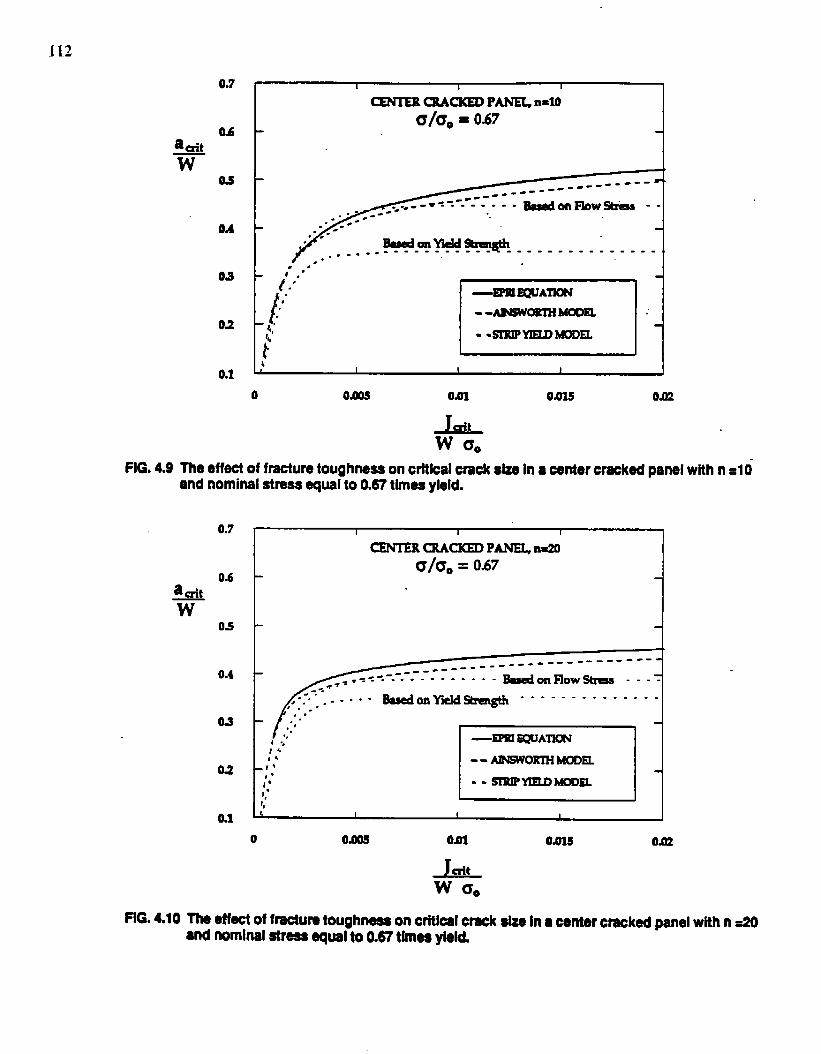
J1.2

0.7

Ma~tw

03

04

03

02

0.1

------ ---

------------- - Bs8dml%wti -‘.

.

.. B&9edunYieuv . . . . . . . . . . . . . .-------- ------- --.

(:”””i!,/’i

I

0 Oms Om Oms O.m

kw aa

FIG. 4.9 The effect of fracturetoughnesson critkalcracksizein ● oentercrackedpand with n =10and nominsistress equalto 0.67 times yield.

0.7 1 I I 1

0.6

0s I1< ------.

0.4------ ----- ------------==-.-+-.--m.-+

~**- “-B8sdon Flowstru14---~

I /----

●“...--. “-kdol’lwdbgt h””” ”----- -----. ..-

1“/..

03 “,‘.,.1’4.”

02 ;;1’l,”1,

-- AnwwoRniMmEL.

-- sIl?lPYxJ3hmDEL

o ems O.ols O=

LW*A.

FIG.4.10 TReetl~ of fracturetoughnesson criticalcrock size in ● centercrackedpanelwithn =20and rmminalstressequaito 0.67 times yield.

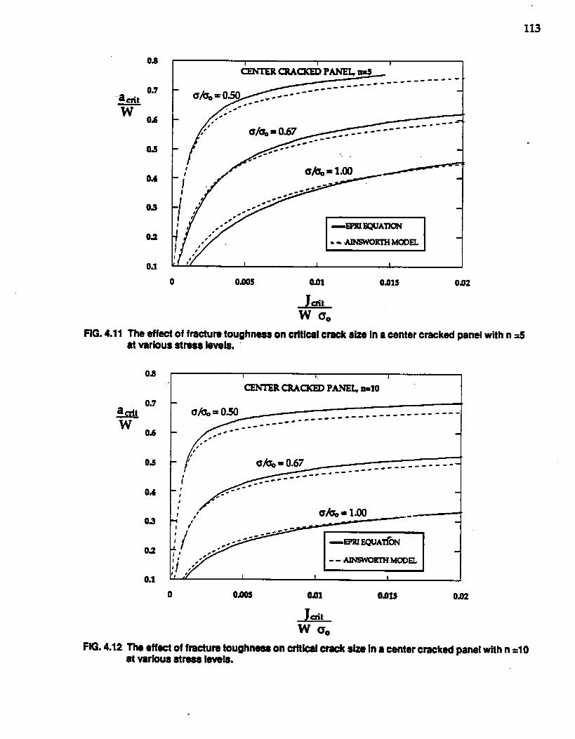
113

. .

FIG.4.11

04

OJ

04

03

02

0.1

cENrERaKKEDPwI!14------------ ---

..

,1’/.I

0 Oms 041 0A15 oa2

ALw 00

The effeci of fracturetoughnesson critld crack size in a center cracked panelwith n ~

O& I I 1

CENTER CRACKED Pm Il=lo

03

04

03

02

0.1

ke/& = t)m ------ ----------------- --------------~-.

,’1’

U&x 0,67 - .-------” -------------

1

o Oms Onl Oms 042

FIG.4.12 The effectof fmcturotoughneeson crfti~ crack size in a center cracked panelwith n =10at varbus stress levels.

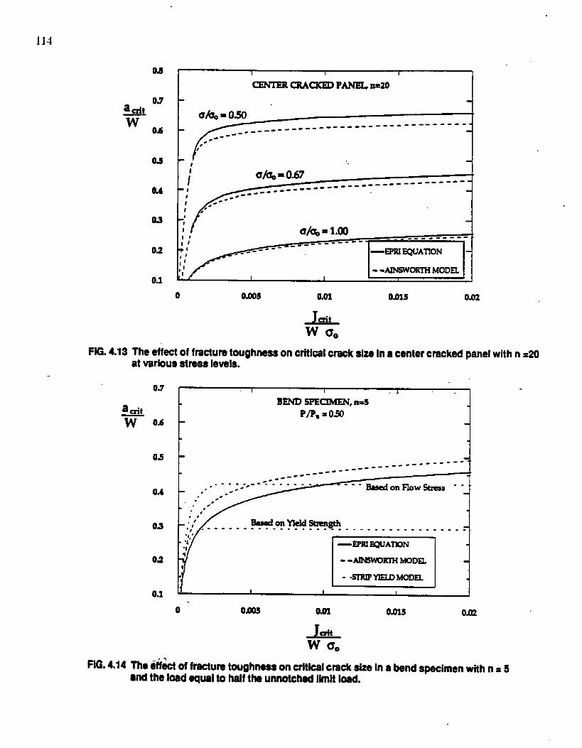
114

Oa

u

OA

03

02

0.1

I I 1

CBNTER cRAcKD3 PANELn=20

a&= Qa

.---= - ----- ------ ----- ------------

f

iu/& = 0.67

,f ------- ----- . . . . . . ------ ------ -It,

I - -A3NWORTH MODEL

o O.oos Om O.ols 0.02

FiG.4.13 The ●ffect of fracturetoughnesson erfticaicrack size in a center cracked panelwith n =20atvarbus stress ieveis.

0.7

0s

0.4

02

0.1

I I I 1 .,I

1=-BEND SPECIMEN,ti

P/P.=050

-.------- ---------------------

..-” .............~- ‘-- BaAon Plow Stms ‘-.“ --. #-. . ..,. ,J -

Y.*)’ d-~--@’$ . . . . . . . . . . . . . . . . .‘f’-----”-” -- ”-------,, .

‘4’,1

—- ~A~N

Q- Om em om5 0.02

JdLw O*

H&4.14The &t of fracturetmghnese on criticsicrack size in a bend specimen with n = 5and the ioad equal to halftheunnotchediimitiosd.

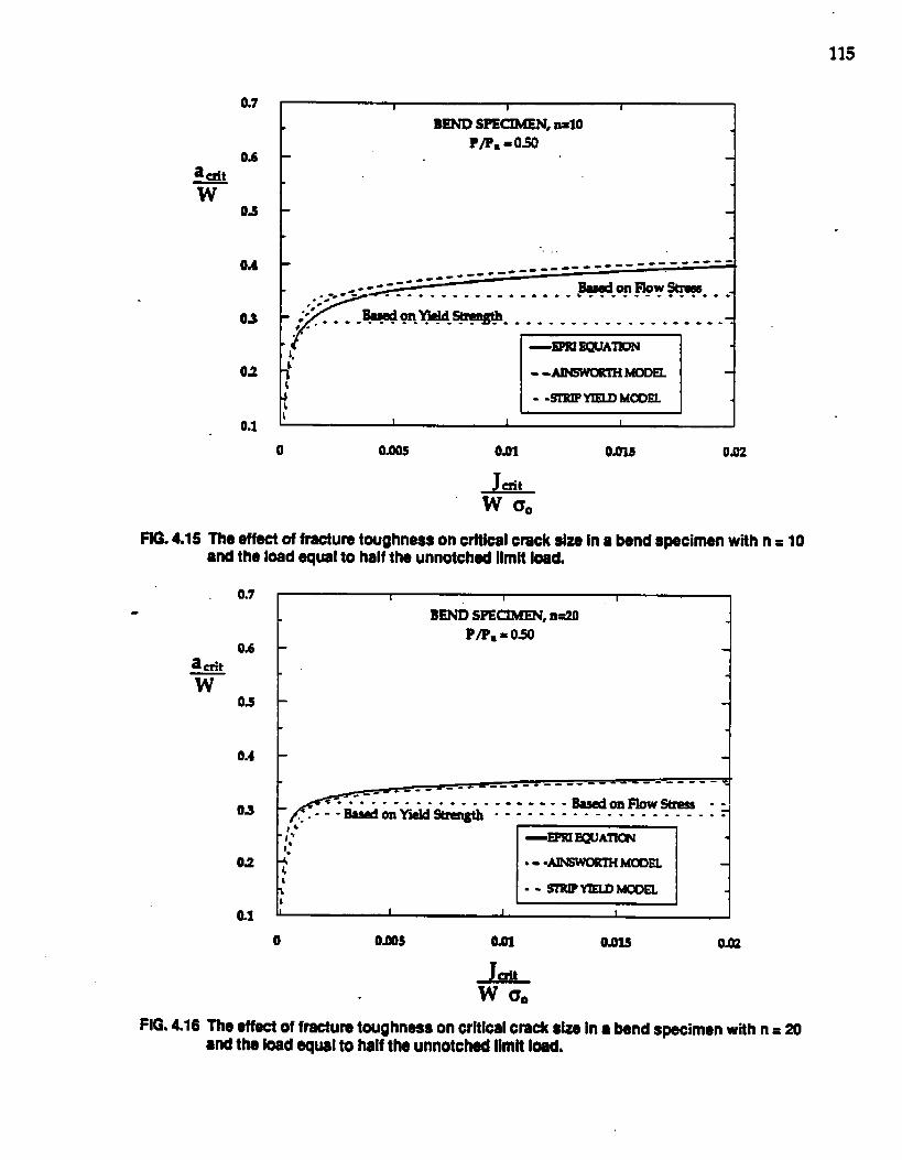
115

0.7

006

0.1

t

BENDSPECIMSN,n=loP/P.=oa I

l“”” ..

I--=...---------:---------------{ Badon How Stm6.-=--+ ------- ---.--- .+ *...- .. ----- ....-

“0 -., .Www.- . .. . . . . . . . . . . . . . . ...7rO*”---

1,—mEawloN

o 0.005 Oal 0415 0.02

FiG.4.15 The effect of frscturatoughnesson critical crocksize in a bendspecimenwithn = 10and the load equalto haif the unnotchd iimit load.

0.7 I I I

BEND SPECIMEN, n=20

P/Pm=050O&

a~t

w03

0.4

-. --+-- ---- .----*--- ----------

“--” ---aa8alon Flow-: &&-y. &&,&&_. . . . . . . . . . . . . . . .,,4

;*

1,~ ~

—= WA-

02 :“ .- -AMWORTHMUXLt -- srRIPrELDMcmL

b

al J I

o oms Oal Oms Om

FiG.4.16 The effm of fracturetoughnesson critioalcrocksize in a bend s~cimen with n = 20●ndthe load equaito haif th unnotchodlimit iosd.

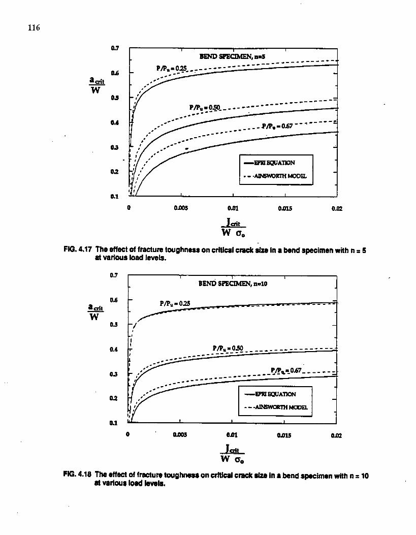
116

BEND mcnKEN, U4 ------ ---- .

pflm:~s””7 -”-””””””””””---””----

●*-

,t

* ------ -#

p~::!a”””” ””””””-”””””””

.PR,=OA7--”-----=4 0-

1 I

1’Ir

0 Oms Oals OJ12

LW%a

FIG.4.17 The effectof fracture toughness on critical crack SIZSin a bend speoimenwith n = 5at various load levels.

O*7 I I IBENDS~CIMEN,n40

0.6a~t P/Pu=02s ------ ---

w0s -~

/’0.4 r Pflu=oq.--.-.--”-----”” --- :

I ----------c1I .-

. . . ..”E4’@~7.”-- ””” .------------

L 1

I,- ~

O.1 I

o ‘ Oms Oals 042

Lw%.

FIG.4.18 The effect of fmcture toughnesson crfticalcraoke&e In ● bend specimenwtth n = 10at verfousload levels,

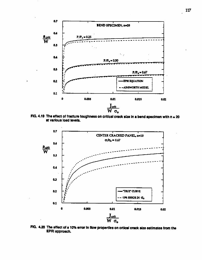
Iv

.

I 1 i

BEND SPECIMEN,a=20

P/P. =02s “------ ----- . . . . . ----- ----- ----- 7.------ -.

#-tI1

-.

II Pm.= 0s* ----------- -----I -----L

1 Pp. - o&7trl

q .

I( ‘,=;I

o oms Om Oms 0.02

FIG.419 The effect of ftiura toughness on critical crack sise in a bend epeoimenwith n = 20d various ioad Ieveie.

0.7 I I 1CENTERCMCKED Pa n=10

a&= 0.6704 7

adtT

1/- ‘

.--- =---- ------- -e ---------

0.s --------~-.-.’ ------ --------- --0 -. -#--

0.4 ● ---z--.’ ----t ---I ~.

1 -.

m. 4a

:/

--

03 - “ ““1’ ●’I #’#

02 -“l’” ,= :

0.1 ‘

o O,ws OJIU 0002

LdLw am

Theeffectof a 10%error in flow propertieson crticai c- sb astimatesfrom theEPRi appiwach.

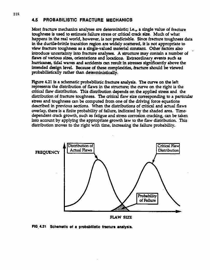
118405 PROBABILISTIC FRACTURE MECHANICS

Most fracture medltardcs analys= are deterministic; Le.,, a single value of fracturetoughness is used to estimate failure stress or uitim.1 aadc size. MuA of whathappens in the real world, however, is not predictable. Since fracture toughness datain the ductile-brittle transition region are widely scattered, it is not appropriate toview fracture toughness as a singkvalued material mnstant Other factors alsointroduce uncertainty into fracture analyses. A structure may contain a numlwr of “flaws of various sh, orientations and lodions. Extraordinary. evenfs such ashurricane, tidal wav~ and acddents can result in stresses significantly above theintended design level. Because of these complexiti~, hcture should be viewedprobabilistically rather than detmrurus“ “ tidy.

Egu.re 4.21 is a schematic probabilistic fracture analysis. The mane on the leftrepresen~ the distribution of flaws in the structure; the cume on the right is theaitical flaw distribution. This distribution depends on the applied stress and thedistribution of fracture touglums. The critical flaw size corresponding to a particularstress and toughness can be computed from one of the driving force equationsd=tibed in previous sections. When the distributions of critical and actual flawsoverlap, there is a finite probability of failure, indicated by the shaded area. Tim-dependent crack growth, such as fatigue and stress corrosion cracking can be takeninto account by applying the appropriate growth law to the flaw distribution. Thisdistribution moves to the right with time, increasing the failure probability.

FREQUENCY

*Distributionof titical Flaw’Actual Flaws Dkibution

FIAwSIZE

FIG.4.21 Schematic of a probablllatlc fractur. mslysls.

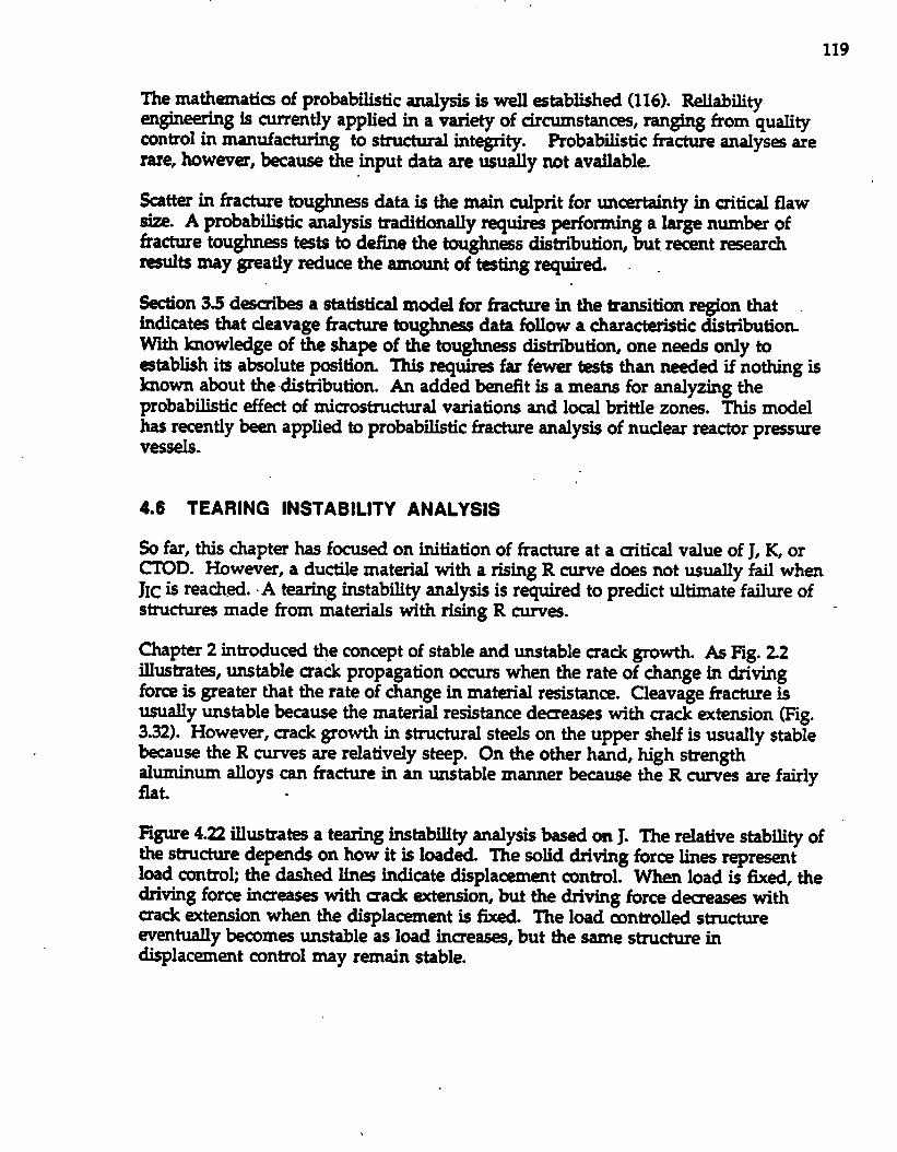
119

The mathe.math of probabilistic analysis is well ~tablished (116). Reliabilityengineering is currently applied in a variety of circumstances, ranging from quality-tro1 in manufacturing to structural integrity. Probabilistic fracture analys werare, however, because the input data are usually not available.

Scatter in fracture toughrws data is the main culprit for uncertainty in mitical flawsize. A probabilistic analysis traditionally requires prforming a large number offracture toughn~s t@s to dei?me the tou~s distribution, but recent r#earchdts may greatly reduce the amount of tdng required. .

Section 35 d=uibes a statistical model for fracture in the transition region thatindicats that cleavage fracture toughn~ data follow a characteristic distributionWith howledge of the shape of the toughn~s distribution, one needs only to=tablish its absolute position. This require far fewer tests than needed if nothing isknown abut thedi.stribution. An added benelit is a means for analyzing theprobabilistic effect of microstructural variations and local brittle zones. This modelhas recently been applied to probab~tic fracture analysis of nuclear reactor pr~urevessels.

4.6 TEARING INSTABILITY ANALYSIS

So far, this chapter has focused on initiation of fracture at a mitical value of J, K, orCTOD. However, a ductile material with a rising R curve does not usually fail whenJIC is rea~~. ~A ~~g ~tability an~ysis is required to predict ultimate failure ofstructures made from mattials with rising R cumes.

Chapter 2 introduced the concept of stable and unstable crack growth. As 13g. 2.2illustrates, unstable mack propagation occurs when the rate of change in drivingforce is greater that the rate of change in material resistance. Cleavage fracture isusually unstable because the material resistance decreases with crack ~tension (Fig.3.32). However, mack growth in structural steels on the upper shelf is usually stablebecause the R tunes are relatively steep. On the other hand, high strengthaluminum alloys can fkacture in an unstable manner because the R tunes are fairlyflaL

Rgure 4.22 illustra~ a tearing instability analysis based on J. The relative stability ofthe stnmture depends on how it is loaded. The solid driving force lines representload control; the dashed lines indicate displacement control. When load is fixed, thedriving force increases with uack ~ion, but the driving force decre~ withcrack extension when the displacement is fixed. The load mntrolled structureeventually becom~ unstable as load incre~, but the same structure indisplacement control may remain stable.

J

..‘ I7hstability.inbad Control

A3●

AaFIG. 4Z Comparison of crock growth resl$tance(heavy Ilne) with driving force In load

COf’ftrOl(sollcl cuwes) Snd dlsplacemont Conttd (dashed CUWOS).

Most structures ~st somewhere between pure load control and pure displacementmntrol. The general case can b represented schematically as a spring in series withthe stnxture, as in Fig. 4.23. In displacement control, the system mmplianm, CW iszero; Le., the system is infinitely stiff. Load control cmesponds to an infinitelycompliant system. Elastic energy stored by the “spring*’helps to drive the mackThus the more compliant the system, the more available potential energy, and the1ss stable the system tends to k.

The bad-displacement behavior of a hypothetical structure is illustrated in Fig. 4.24.If the stmwture is load controlled, it becomes unstable at the maximum load plateau.In pure displacement control, the stmcture remains stable, even after significantamounts of mack growth. At the intermediate rendition, instability occurs aftermaximum load.

Paris and Hutchinson (117) have developed a detailed instability analysis for ductilematerials that takes account of system compliance. Their approach has &ni.ncorprated into the EPRI elastic-plastic frachare handlmok.

Paris and Hutchinson introduced the concept of the stability assessment diagram.Their approach requires that slop of the driving force and resistance cun~ benondiinensionalized by means of the tearing modulus. The tearing modulus for thematerial is defied as

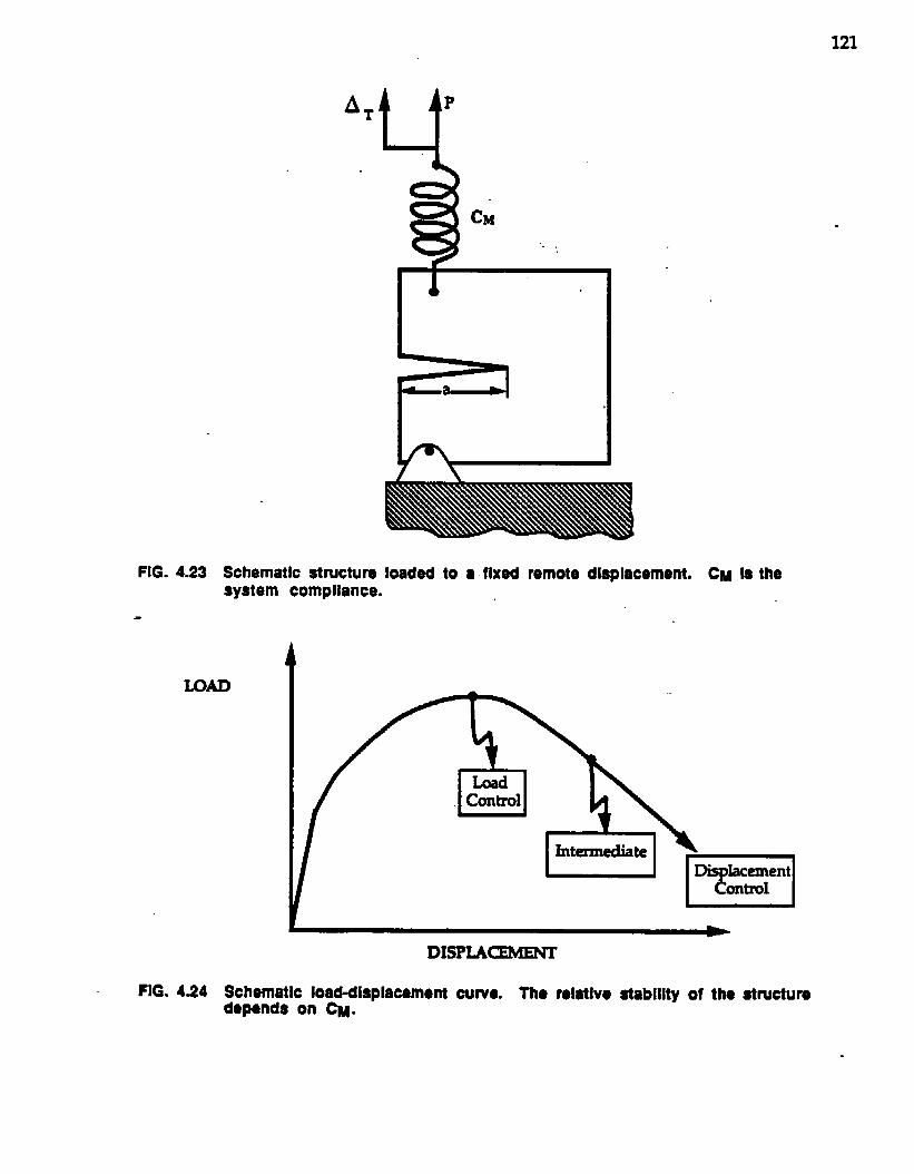
121

A=U P

FIG. 4.23 Schematic structure loaded to ● flxad remotesystem compliance.

displacement. CM Is the

FIG. 424 Schematic load-displscemo~ cume. TkM rolatlve atabilitv of the structuredepends on CM. -

.

122

where JR is the value of J on the R -a The applied T depends on the partialderivative of J at a i5xed remote displacement

-. E4351lhe conditions for stable and unstable sack extension areas follows. “

*TJ < T~ (stable) [-

The above conditions for stability are analogous to those presented in Chapter 2 forI.inear elastic conditions (Eq. [2.2]). The partial derivative in Eq. [435] is obtained froma rather complex expression: .

(3..=(3,-[~)a~)P[cM+&)~]”l[43n

Each of the terms in the above expression is obtained separately from therelationships for P, A, and J in the EPRI handbook. The computation is laborious ifdone manually; but for most practical situations, one can make the consemativeassumption that the structure is load controlled and CM = -, simplifying Eq. [4.37]considerably:

(%=(:), [438]

The situations in which one would perform a complete analysis with Eqs. [434] to[4.371 are rare. As illustrated in in 13g. 4.4, instability occurs after maximum load ifthe system compliance is iinite, but no competent d~igner would let a structure togo beyond limit load under nomnal semice conditions. The only time a detailedtearing analysis is appropriate is for prediction of the behavior of the structure underextraordinary loading. The above approach was originally developed to analphypothetical accidents in nuclear reactors. Actual semice stresses in a reactorpr=ure v=sel are low enough to ensure that the structure is loaded well below theJIC of the material.

123

4.7 SIMPLIFIED ELASTIC-PLASTIC ANALYSES

Complete tearing instability s.nalyss can be extremely complex and there is noguarantee of accura~, since computed J valu~ are highly sensitive to the input data(Section 4.4). Even the thr-ti= approach can be complicated.

There are many i.nstan~ when simple screening uiteria would be useful. Theanal- in Section 4.4 illustrate that if fracture toughn~s is above a certain level, -sinmtural failure is controlled primarily by the material’s flow propertb. In suchcases, the d=igner can avoid failure merely by ensuring that the slmcture is str~sedwell below its limit load. Thus one purpose of a fracture toughn~ screeningcriterion is to define the lmmdary Mween collapse controlled failure and fracture

- controlled failure.

Two simple fracture toughness saeening dteria have been been published recently(71,118). One approach pertains to fracture initiation, either by cleavage or ductiletearin~ and the other relates to teazing instability.

4.7.1 The Yield-Before-Break Criterion

The Yield-bforebreak criterion (71) is analogous to the leak-bforebreak approach, atoughn~s criterion desigrted to ensure that a mack in pressure vessel or pipe growsthrough the wall Wore it becom~ unstable. A its name suggests, the yield-beforebreak criterion quantifk the required level of toughness to ensure that fractureinitiation occurs after net section yield.

Consider a structure that contains a surface flaw of depth a. If the flaw is smallcompared to the total uoss section of the structure, the ~OD at net section yield canb estimated con$ematively from the following equation.

~m2 a8NsY=~ (125 &y+ 0.002)

where Mm and $ are as defuwd in Eq. [4.25]. This equation was derived from therefererm stress approach This simple ~ult was obtained by assuming nomimals-s, reference str~, and yield strength are equal.

The yield-befor~break concept can be illustrated with a simple example. If a 2S mm(1.0 in) thick plate contafns a semicircular surface flaw 12 mm deep, 6NW = 0.09 mm,a.SS~g ~ = 0.(N)2 Thus if the material u at le~t W ~ugh, me $~~e @ notfail, as long as the applied str- are below yield.

Equation [4.39] can be retied to take account of r~idual str=~ and str=sconcentration effects. If yield magnitude residual stresses are present and there is almal stress concentration, kb the yield-beforebreak CIOD is given by

~w. k? Mm?a—== &y+ 0.002)

#[440]

This mOdMed equation is based on a number of conservative assumptions~~e.he it ~ tend to Over=timate ~NW.

A word of caution is necessay when applying ~ approach in the tmnsition regio~Since cleavage fracture toughn=s data in the transition region me invariablyscattered, it it is not s@cient for the average toughness to b above the yield-befor-break -hold. In order IOensure a high probability of yield-bforebreakconditions, the d=igner should compare a luur bound toughness (from Table 3.1)to ~fi.

4.7.2 Critical Tearing Modulus

Not ordy d- the reference str~s model simplify fracture analyses in the transitionregion, it can also simplify tearing instability analysis. Anderson et al. (118) showedthat it is possible to obtain closed-form solutions for ductile fracture in a number ofsimple configuration These solutions can de.fme the boundary between fracturecontrolled failure and collapse controlled failure on the upper shelf.

Consider a center sacked psnel in plane strain. The following closed formexpression was derived for the @ical tearing modulus at maximum load

[4.41]

By tig the ratio crn/~, it is possible to calculate the necessary tearing modulus toreach an. Rgu.re 4.25 is a plot of sample calculations with Eq. [4.41] The net section

str= was H at yield and 10% above yield. The flow property constants n and awere 6xed at 10 and 20, rqectively. According to this plot, the structure will reachnet section yield before tearing instabtity, as long as the crack is small relative to thewidth and the mataial’s tearing modulus is greater than approximately 10. Sincetypical stnwtural steels have tearing moduli greater than 50, nearly all stelstructures a the upper shelf must completely yield kfore tearing instability is apossibility.

A similar expression to Eq. [4.41] has been d~ved for surface flaws (71). Thecomputed TCvalues are similar to the center sacked results.

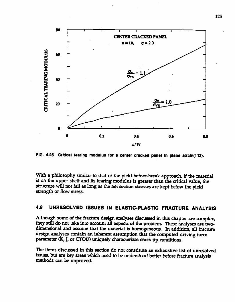
125

80

w

40

20

0

CENTERCRACKEDPANELns 10, a =2.0

.

.

0 02 0.4 0.6 0.8

●lw

FIG. 4.25 Crltlcal tearing modulus for ● center crackad panel In plan. atraln(l12).

With a philosophy similar to that of the yield-befor-break approach, if the materialis on the upp= shelf and its tearing modulus is greater than the aitical value, thestnxtu.re will not fail as long as the net section stresses are kept below the yieldstiength or flow stias.

4.8 UNRESOLVED ISSUES IN ELASTIC-PLASTIC FRACTURE ANALYSIS

Although some of the fracture d-ign analp discussed in this chapter are mmpl~,they still do not take into account all aspects of the problem. k analy~ are tw~dimensional and assume that the material ia homogeneous. In addition, all fracturedesign analys~ contain an inherent assumption that the computed driving forcepu=@er (K, J, or CT’OD) uniquely Charactm sack tip conditions.

The items discussedin thissection do not constitute an exhaustive list of Unr-lvedissues, but are key areas which need to h understood better bfore fracture analysismethods can be improved.

It should be noted that cument methods of fracture analyses are generally safe. Theeffects discussed lwlow tend to make current predictions consemative. A betterunderstanding of these complexities would m~ely make analyses of dicalconditions more accurate. . -

4.8.1 Drlvlng Force in Weldmenta

A steelweld invariably has different flow properties than the parent metal. In most~, the yield strength of the weld metal overmatch= that of the parent metal,although undermatching somedrn~ occurs. Anal- “such as the EPRI approach areunable @ handle structures whose flow propertk are heterogeneous. If a aa~occurs in or near a weld, it is impossible to determine the driving form accuratelywithout performing an elastic-plastic finite element analysis of the componenk

This problem can be illustrated by sting an example from Ref. (112). Three weldedsluminum center ffacked panels were fabricated, with the weld metalundexmatching the strength of the parent metal. The sack in each panel was in theweld, which ran perpendicular to the loading direction. NarTow strips were extractedtim each weld for tensile t~ting. Each tensile spedmen was loaded perpendicularto the welding axis, so as to be representative of loading in the wide plates. The gagesection contained parent metal on either side of the weld. A strain gage wasmounted on the weld to measure the effective flow propertk of the weldment.These flow properties, along with crack growth resistance cures from small despedmens, were used in conjunction with the reference str~s model to perform atearing analysis of each wide plate specimen. These ar@yses underestimated thefailure stress by as much as 32%, despite extra care in measuring the true flowproperties of these panels. ‘Ihe apparent ~lanation for the discreparq is that theweld metal in the narrow tensile spedmens was 1=s constrained than in the wideplates. Hence the effective yield strength was higher in the wide panels.

4.8.2 Residual S~resses

lhe assumptions for secondary stresses have a significant effect on predictions witheither the R-6 method or PD6493, but accurate information on the distribution of-dual str=- is rarely available for the weld in qu~tion.

Conventional methods for measuring the through-thickness distribution of r~idualstr~s are d~tructive. Material from one side of the welded plate is typically ‘.removed by a milling machine while strain gage readings on the other side of theplak are recorded. Such an approach is obviously impractkd for a structure insewice. The center hole drilling tedmique does minimal damage to the structure,but it only provid~ information on the surface stresses. The only available methodfor through-thickn~ residual str~s measurement is neutron diffraction, atechnique is not portable.

127

A reliable, ptable, nondestructive method for measuring residual sh=ses isckperately needed. Accurate ~te ek+nent mdels that predict the residual str~sdistribution from the joint geometry and welding procedure are also ddrable.

4.8.3 Thres-Dlmenslonal Effects

Existing elastic-plastic analp do not account for the variation of the driving form .ting the ma~ front Parks (113) has conducted munerical studies and Reut~ et d(114) have @ormed experiments that demonstrate that lmth J and CTOD varyconsiderably along the tips of surface flaws Thus the uack tip conditions cannot beuniquely diaracterizd with a single value of J m ~D.

‘Rt- thr-ensional “effects influence both cleavage and ductile tearing. Siicecleavage is statistical, good predictions will come mly from sumdn g theirmemental failure probabilities along the ~ack front. Such a calculation must takeaccount of the variation in the sack driving hrce with positiom Since ductile mackgrowth =CLUSfastmt where the driving force is highest, accurate tearing predictionsare possible only with a three-dimensional analysis.

4.8.4 Crack Tip Constraint

Constraint is related to the thrtiensional issue. Plane strain fracture analysesassume that J or CTOD uniquely &aract_ sack tip str~ and strains. If theentire crack front is not in plane strain, however, there are regions where a singleparameter does not characterize mack tip conditions. Similarly, the single parameter

. assumption breaks down under large scale plastiaty, which d-ease the crack tipconstraint. This constraint 10SSam occur at very low J (or CTOD) valu~ instxuclams loaded predominantly in tension (see Section 3.5.2). In such cases, thestructure has a higher apparent toughness than the small scale fracture toughnas-b, which were loaded predominantly in kd.ing.

The experiments and analyses of surface sacks by Reut= et al. (120) and Parks (121)demonstrate the complexities of constra.in~ The apparent driving force, quantifiedby either J or CTOD, wss highest at the maximum mack depth; i.e., along an axis~~~ tO ~ p~~ fiacec ~ J ~d ~D valus decreased smoothly alongthe sack bent, reaching a minimum at the frm surface, but the maximum crackgrOwth occurred aIong an axis approximately 45° from the free surface. Parks’ finiteelement analp indicated that this was also the l~ation of the highest normals~, even though J and CI’OD were highest at the maximum crack depth. Thecrack tip constraint had apparently relaxed at the point of maximum depth, whichwas close to the back surfa~ of the plate Because of constraint effects, the high~ttie driving force and the maximum apparent driving force were at two differentlocations.

4.8.5 Gross-Section Yielding

l’lie praence of a =ack reduces the cross section in the stmcture; the net section isdefined as the portion of the aoss section not occupied by the ~ack Net-sectionyielding ref- to the @nt when the plastic zone spreads throughout the net crosssection. Gr~ ●on yielding occurs when plastidty encomp~ the entire moss -section. ..

Net-sedon yielding tends to occur with deep sacks, while gross section yielding ismore common with shallow flavs. Since deep mwks are usually avoided instructures, gross-section yielding is much more common. Unfortunately, mostelastic-plastic fracture anal- are not equipped to handle this type of defonnatiom -

Elastic-plastic fracture analyses such as the EPRI and R4 methods assume net-sectionyielding in the stmcture, and are consemative when gross-section yielding occurs.According to the EPRI approach, J in the fully plastic range should scale with P+l.‘However, experimental results of Read (121) indicate that gross-section yieldingcausa the applied J to irmesse much more gradually than qected. Thus an elastic-plastic fracture analysis an greatly overestimate the applied J in the case of gross-section yielding. Reads results indicate that gross-section yielding is most likelywhen the mack comprises less than 5% of the cross section.

129

5. DISCUSSION

This chapter is intended to provide a prspedive.on the state of the art in elastic- “plastic fracture mduinb. Many of the issue rti in Chapters 3 and 4 arediscussed Mow. Where appropriate, recommendations for fuhire directions aremade.

The field of fracture mechanh is relatively mature The CI.UTentstate of technology.is suflkiently advanced to make a major contributionto industry. Not all of theimportant questions have been answered. But enough is known to apply fracharemechanie to practical situations.

One sign of the field’s maturity is that all of the simple problems have been solved;thosemake

5.1

that remain are very mrnplex. Future resear&rs-must be very ~eative tosignificant contributions.

FRACTURE TOUGHNESS TESTING

Chapter 3 demonstrates that the KIc test is of limited value for testing low- andmedium-strength steels. If a steel can satisfy the size requirements of ASTM E399-83(25), it is probably tw brittle for structural applications. Thus fracture toughrws insuch materials must be quantified by elastic-plastic tests.

Fracture toughness testing procedur~ for materials on the upper shelf are well=tablished. The JIc and J-R awe standards (26, 50) provide guideline formeasuring the material’s resistance to ductile fracture initiation and crack growth.One problem receiving some attention is the crack growth limits in ASTM E1152-87.Ernst (122) proposed a modified J integral, which has been moderately successful inproduchg geometry independent R cum- lxyond the normal crack growth limits.This r~arch is driven primarily by the nuclear industry, where accurate tearinginstability analyses are important, but this problem is only marginally important tothe rest of the welding fabrication comnuuiity.

.-

Just as materials that satisfy the KIc size aiterion are usually tcm brittle, materialsthe up~ shelf are sufficiently tough so that fracture is not often a signMcantproblem The fracture r~ch area most important to the welding fabricationindustry is the ductbbrittle transition region.

on

Until recently, the transition region has received little attention from the fracturemechani~ community in the United States. The CX’013 standard (51), the fiststandardized method which can be applied to the transition region, was published in

130

1989by ASTM, whereas the Briiish Standards Institute published a CTOD stand~d in1979, and ~OD data were applied to welded stmctur= 15 years earlier.

Because J integral t-t me@ds w~e originally developed for the upper shelf, there isno standard@d J-based -t that appli= to the transition region. Such a standardshould b developed so that J-based driving force approach= can ~ applied tostructures in the transition region.

-.

One problem with both J and ~D testing in the transition region is the lack of sizecriteria to guarantee a single parameter characterization of fracture. The JIc sizerequiremen~ are probably not r~trictive enough for cleavage, and tie KICrequirements are too severe for elasti~plastic fracture parametm. The appropriatesize requirements can & @abEshed through a combination of i?nite elementanalysis and mimomechani~ modds, such as that deaibed in Section 3.5.

When a single parameter description of fracture toughness is not possible, as inshallow notched spedmens and tensile panels, the issue of crack tip constraintbecomes important. This is a very Mcult problem. Unless a simple analysis isdeveloped that characterizes constraint loss, these effects will be impossible toquantify without performing three-dimensional, elastic-plastic finite elementanalyses on every configuration of interest. The twmparameter approach describedin Section 3.5.2 shows some promise but requires further study.

Another important issue is fracture toughness t~ting of weldments. Existingstandards do not address the special considerations required for weldment t~ting. ~ .The Welding Institute and other organizations have developed informal proceduresover the years, but they need to be standardized.

Fracture toughness data in the transition region are invariably scattered, whether thetests are pdorrned on welds or base materials, although the problem is worse in theheat-affected zone of welds. The nature of scatter in the lower transition region isreasonably well understood; procedures have been developed which allow for ‘estimating lower-bound toughness with as few as three fracture toughness values.The problem of scatter in the upper transition region is more complicated; constraintloss and ductile sack growth combine to increase the level of s=tter. Further workis necsary to quantify th~ effects.

h accuratemrrelation k- Charpy energy and fracture toughness would beexiremely useful. The empirical correlations developd to date are unreliable. Someprogress has been made in developing tlumretical correlations, but these models donot take into account all factors. If an amurate relationship can be developed,material toughn~s uiteria based on Charpy energy can be ~tabli.shed rationally.

131

5.2 APPLICATION TO STRUCTURES

Although linear elastic fracture mechank is of limited use in fracture toughness-ting of structural steels, LEFM driving force relationships are suitable for manysituations. A structure of inter~t, if it is sufficiatly large or thes~ are low, mayb subjected to nearly pure linear elastic conditions. Fracture toughness can becharacterized on a small spcimen by a uitical J value, which can then be converted “to an equivalent KIc and compared to the applied K1 in the structure.

Pure LEFM analysis does carry risks, however. If the Sk are almveapproximately half the yield strength, plastiaty effects can be sigrdkant. If the LEFManalysis d= not mntain some type of plastiaty correctio~ it giv~ no warming whenthe linear elastic assumptions become sus~ %.fikient skill is necessaxy todetermine whether or not an LEFM analysis is valid in a given situation.

It is perhaps better to apply an elastic-plastic driving force relationship to allproblems; then, the appropriate plastiaty corrections are available when needed.When a linear elastic analysis is acceptable, the elsstic-plsstic approach wiJl reduce tothe LEFM solution. Thus the analysis decides whether or not a plastidty correctionis needed.

Several types of elastic-plastic fracture analyses are available. The ~D d~ign-e, based primarily on an empiricsl comIation between wide plate tests andCIOD data, is largely obsolete. Analyses based on the strip yield model are stilluseful for low hardening materials. The EPRI procedure is the probably the mostadvsnced snslysis, but it is currently applicable to a limited range of con@rations.The reference stress model, which is a retied version of the EPRI approach, iswidely applicable. Any of th- approa~~ can be expressed in terms of a failure_sment diagram. This is done merely for convenience, and has no significanteffect on the outcome of the analysis.

The parametric study in Section 4.4 produced some interesting results. A ~ected,the strip yield, Ainsworth, and EPRI analy~ all agreed in the linear elastic range. Inthe elastic-plastic and fully plastic rang=, where the three analyws might b ~ectedto differ, predictions of failure str- and cxilical cra~ size were quite dose in mostcases; the only =Ception was whan the strip yield model w.s applied to the highhardening (n=5) material. All the anal~ predicted similar failure str~ anduitical mack sizes Iwcause failure in the fully plastic range is governed by the flowpropertk of the material. Almve a certain level of toughness, dical valu= of str~sand crack size are insensitive to fracture toughness.

The analy~ do differ in the prediction of the applied J, but for a designer, miticalcrack size and failure stress are much more important quantitk. Accuratepmdktions of the applied J may ~ ixrpssible, &en with an analysis that istheoretically p~ect. The applied driving form in the plastic range is highly sensitive

to the P/P. ratio. A slight over=timate or under-timate of PO significantly effectsthe ra.dts. If the flow properties vary even by a fw ~cent, the r=ulting emor in POleads to a large error in the J calculation.

In summary, the driving force expression probably does not matter in most cases.The only requirements are that the exprssion reduce tn the IXFM solution for smallscale yielding and predict the correct collapse limit under large scale yielding “ccmdiiions. An additional proviso is that the stip yield approad or otherrmnhardening models should not be applied to high hardening materials.

Since the Ainsworth mcdel works as nearly wdl as the EPRI approach, there is littlejustMcation for the EPl?I approach in non-nuclear applications. The EPRI procedureis more cumbrsome because it requir~ a folly plastic geometry correction factor.The Ainsworth model produces similar ~ults to the EPRI analysis and has theadvantage of a geometry factor basad on str~ intensity solutions. Currently, thereare many more published K solutions than hl solutions.

There areothernot to wony about applying accurate plastic geometry factors. Realstructures, especially welded structures, pose many cornpl~ problems that existinganalyses cannot address. As Section 4.8 indicates, the elastic-plastic driving force in aweldment cannot be represented accurately by a solution for a homogeneousstructure. Additional factors such as r~idual stresses, thedimensional effects, andcrack tip constraint, and gross-section yielding combine to increase the uncertaintyand potential errors in fracture analys~. These errors are mudi more signMcantthat those that might arise from choosing the strip yield or Ainsworth analysis overthe EPRI approach Until the compkities discussed in Section 4.8 an be addr~se~one may as well adopt a simple elastic=plastic analysis.

As a fist step in a fracture analysis, a simple scr~g criterion may be appropriate.Two such approaches are introduced in Section 47. ‘Ihe yield-beforebreak uiterionStimates of the level of tougluws required for the structure to reach net sectionyielding &ore fracture initiation. If the toughness is adequate to ensure yield-Hor-break conditions, fracture can be avoided simply by ensuring that the structureis loaded well below its limit load. An analogous quantity, the uitical tearingmodulus, is d~igned to ensure that the tearing resistance is adequate to avoid atearing instability below the limit load.

6. CONCLUSIONS AND RECOMMENDATIONS

6.1 FRACTURE TOUGHNESS TESTING .

●

●

●

●

●

✎ ●

●

KIc -ting is of little value for stnwtuml steels. Fractui’etoughrms shouldk quantifid by elasti~plsstic parameters such as J and ~D.

The ductil+brittle transition region is the critical area of concern in weldedsteel structure. If a material is on the lower shelf of toughn-s, it is bbrittle for structural application If the material is on the upper shelf,fracture is not a significant problm

A standard for J testing is the transition region should be developed.

Size requirements for both J and ClOD measurements in the transitionregion should be established. Constraint loss should be quantiikd for caseswhere these size requirements are violated.

Sticient semice germ exists to develop a standard for weldmenttesti.n~ which is desperately needed

The nature of scatier in the lower transition region is understood reasonablywell. Further work is nec~sary to characterize the upper transition region,where uack growth and constraint loss inmease the level of scatter.

Accurate snd reliable correlations between Charpy energy and fracturetoughness are not available.

6.2 APPLICATION TO STRUCTURES

●

●

●

Many slructurs behave ina linear Astic manner but it is safer to apply amore general analysis that corrects for plastiaty when necessary.

Predictions of critical sack size and failure ~ are insensitive to thedriving force equation. .

Of the available ehstic-plastic driving force relationships, the strip yieldmodel and the Ainsworth reference stress approach are the most suitable forwelded steel structures, but the stdp yield model should not be applied tohigh hardening materials.

134

● If the toughnm of the material is above a certain level, failure of thestructure is controlled by the flow propertk of the mataial ratha than thefracture properties. Simple approach- to estimate the required toughn~sfor collapse controlled failure are available.

● Future ~ch should focus on a number of areas, including driving forcein welded structures, residual str~s measurements, thr-ensional -effects, sack tip constraint, and gros~on yielding.

135

7. REFERENCES

1.

z.*

3.

4.

5.

6.

7.

8.

9.

10.

11.

12

~n, J.D., Gamoui, S.J., and Daw~, M.G. “Case Studies and Failure -Prevention in the Petrochemical and OffMore Industry.” Presented atFracture 84, 2nd National Conference on Fracture, Johannesburg SouthAHca, Novernhr 2M8, 1984.

Griffith, A.A The Phenomena of Rupture and Flow in Solids.”Philosophical Transactions, Series A, Vol. 221, 1920, pp. 163-198.

Irwin, G.R, ‘Onset of Fast Crack Ropagation in High Strength Steel andAluminum Alloys.” Sagamore Rmarch Conference Proceedings, Vol. 2, 1956,pp.289-305.

Westergamd, H.M., “Bearing Pressures and Cracks.” Journal of AppliedMechanics, Vol. 6,1939, pp. 49-53.

In@ G.R, “Analysis of Stresses and Strains near the End of a CrackTraversing a Plate.” ]oumal of Applied Mechanics, Vol. 24, 1957, pp. 361-364.

Wfiams, M.L., “On the Stress Distribution at the Base of a Stationary Crack.”Journal of Applied Mechanics, Vol. 24, 19S7, pp. 109-114.

Brom W.F. Jr. and Srawley, J.E., “Plane Strain Crack ToughnessTding of High Strength Metallic Materials.” ASTM SIT 410, 1%6.

Rooke, D.P. and Cartwright, D.J., Compendium of Stms IntensityFactors. Her Majaty’s Stationary Office, London, 1976.

Tada, H., Paris, P.C., and ~, G.R The Sties AnaZysisof CrackHandbook. Del -arch Corporation, Hellertown, Pa, 1973.

MLuakarni, Y. Stress Intensity Factors Handbook Pergamon Press,New York, 1987.

Imin, G.R, “Plastic Zone Near a Crack and Fracture Toughness.”Sagamore Research Conference Proceedings, Vol. 4, 1961.

DugdaIe, D.S., Tielding in Steel Sheets Containing Slits.*’ Journal ofthe Mechanics and Physics of Solids, Vol 8, pp. 100-104.

136

13. Barmblatt, G.I., “The Mathematical Theory of Equilibrium Cracks inBrittle Fracture.” Advances in AppliedMechanics, Vol VII, AcademicR-, 1%2, pp. 55129. .

M. Wells, AA., %hstable .Cra& Ropagation in Metals: Cleavage and FastFracture.” Proceeding of the Crack Propagation Symposium, VO1 1,Paper 84, Cranfmld, ~ 1%1.

..

15. Rice, J.R “ A Path Jndepndent Integral and the Approximate Analysisof Strain Concentration by Notches and Cracks.” @umal # A#iedMechanics, Vol. 35,1968, pp. 379-386.

16. Hertzberg, RW., Deformation and Fracture of Engineering M&&. ThirdEdition, John Wiley & Sons, New York, 1989.

17. Tuba, LS.., “A Method of Elastic-Plastic Plane Stress and StrainhdySiS.n Joumd of Strain hdySiS Vol. 1, pp. 11S122, 1966, asreferenced by Broek, David, Elementary En#”neering FractureMechanics (4th cd.), Kluwer Academic Publishers, Nonvell, MA, 1988.

18. Burdekin, F.M. and Stone, D.E.W., “The Crack Opening DisplacementApproach to Fracture Mechanics in Yielding Mat~ials.” Journal of StrainAnalysii, VOL 1, 1%6, pp. 144-153.

19. Eshelby, J.D., “The Continuum Theory of httice Defects.” Solid State Physics,vol. 3,1956.

20. Hutchinson, J.W., “Singular Behavior at the End of a Tensile Crack Tip in aHardening Material.” Journal of the Mechanics and Physics of Solids, Vol. 16,1968, pp. 13-31.

21. Rice, JR. and Rosengren, G.F., Plane Strain Deformation near a Crack Tip in aPower-Law Hardening Material.” Journal # the Mechanics and Physics ofsolids, Vol. 16,1968, pp. 1-12

22 SMh, C.F. “Relationship between the J-Integral and the Crack OpeningDisplacement for Stationary and Extending Cracks.” Journal of fhe Mechanicsand Physics of Solids, Vol W, 1981, pp. 305-326.

23. Anderson, T.L me Effect of Crack-rip Region Constraint on Fracture in theDuctil~to-Britde Transition Region.” Ph.D. Dissertation, Colorado School ofMines, Golden, CO, October, 1983.

137

24. McMeekin& RM. and Parks, D.M., ‘On Criteria for J-Dominance of Crack-~pFields in brg4cale Yielding.” ASINf SIP 668, American Society of Testingand Materials, Philadelphia, PA, 1979, pp. 175-194.

25* E399-83, Standard Test Method for Fracture Toughnes of Metallic Materials.”American Society for Tdng and Materials, Philadelphia, PA, 1983.

26. E813-87, “Standard Td Methd for JIO a Measure of Fra@re Toughness.”American Society for Testing and Materials, Philadelphia, PA, 1987.

27.- Wellman, G.W., Sorem, WA., Do&is, Jr., RIZ, and .Rolfe, S.T., “SpecimenThickness Effects for ElastiePlastic CIOD Toughn~s of A36 Std” ASTM STP945, American Society of T~ting and Materials, Philadelphia, PA, 1988 pp. 53%554.

20. Knott, J.F., “Mimomechanisms of Fracture and the Fracture Toughness ofEngineering Alloys, Fracture 1977, Vol 1, ICF4, Waterloo Canada, June 1977,p. 61.

29. Fra.ctdgraphyand Atlas of Fraitographs, Metsls Handbook, Eight Edition,Vol. 9, American Soaety for Metals, Metals Park, Ohio, 1974..

30. McMahan, C.J. Jr and Cohen, M., Initiation of Cleavage in PolyaystallineIron.” Acts Metiallurgica, Vol 13, 1%5, p. 591.

31. Smith, E., The Nucleation and Growth of Cleavage Miaoaacks in MildSteel.n Proceedings of the Conference on the Physical Basis of Fracture,Institute of Physi= and Physi~ -ety, 1966, p. 36.

32. Cottrell, A.H., “Theory of Brittle Fracture in Steel and Similar Metals.”Transactions of the ASME, Vol 212, 1958, p. 192

33. Dolby, RE. and hot-t, J.F., Journal @ the Iron and Steel Institute, Vol 210,1972, p. 857.

34. Gerkmrich, W.W. “Metallurgical Aspects of Crack ~p Failure Recesses.”ASTM STP 945, American Society of Tdng and Materials, Philadelphia, PA,1988 pp. 5-18.

35. Lin, T., Evans, AG. and RitcMe, RO., Statistical Model of Brittle Fracture byTransgranular Cleavage.” @unwl of the Mechani~ and Physics cf Solids, Vol34,1986, pp. 4774%.

36. Imin, G.R, Prmtation at the meetings of ASTM Committee E24 on FractureTestin~ -O, NV, Aprii 1988.

138

37.

38.

39.

40.

41.

42-

43.

44.

45.

46.

47.

Ritch.ie, RO, Knott, J.F., and Rice, J.R “On the Relationship betwti CriticaITensile Stress and Fracture Toughness in Mild Steel.” Journal ~ iheMechanics and Physics of Solids, Vol. 21,1973, p. 395.

Curry D.A and Ktoti, J.F., “Effect of Microstructure on Cleavage FractureToughness in Mild Steel.” Metal Science, Vol. 13,1979, p. 341.

Cuny, DA, “Comparison &tween Two Models of Cleavage Fracture.” MetalScience, Vol 14,1980, p.78.

Wallin, K, SaariO, T., and T6rrdnen, K, “Statistical Model fbr Carbide Induced “Brittle.Fracture in Steel.” Metal Science, Vol. 18,1984, p. 13.

Berernin, F.M., “A Local Criterion for Cleavage Fracture of a Nuclear pr~sureVesel Steel.” Metallurgical Transactions, Vol. 14A, 1983, p. 2277.

Evans, A.G.. “Statistical Aspects of Cleavage Fracture in Steel.”, MetallurgicalTransactions, Vol. 14A, 1983, p. 1349.

Ander~n, T.L., “A Combined Statistic~/Cofitraint Model for the DuctikBrittle Transition Region.” ASTM STP 995, American Sodety of Testing andMaterials, Philadelphia, PA, 1989, pp. II-563 - II-583.

Anderson, T.L. and Stienstra, D., “A Model to Redict the Sources andMagnitude of Scatter in Toughness Data in the Transition Regiom” Journal@Testing and Evaluation, Vol. 17, 1989, pp. 653.

Rim, J.FL and Tracey, D.M., “On the Ductile Enlargement of Voids in TriaxialStress Fields.” Journal o/the Mechanics and Physi~ of Solids, Vol. 17, 1969,pp. 201-217.

d’Escata, Y. and Devaux, J.C., ‘N.unerical Study of Initiation, Stable CrackGrowti, and Maximum Load with a Ductile Fracture Criterion Based on theGrowth of Hole.” ASI’M STP 668, American %ciety of Testing and Materials,Philadelphia, PA, 1979, pp. 229-248.

Devaux; J.C., Rousselier, G., Mudry, and Pineau, ““AnExperimental Programfor the Validation of Local Ductile Fracture Criteria Using ~etricallyCracked Bars and Compact Tension S@mens.” Enginm”ng FractureMechanics, Vol. 21,1985, pp. 273-283.

Heerens, J. and Read, D.T., “Fracture Behavior of a fiessure V@ Steel in theDuctil~t&Brittle Transition Region.” NISTTR 88-3099, National Institute forStandards and Tdnol~, Boulder, CO, December, 1988.

.

139

49.

50.

51.

52.

53.

54.

55.

k.

57.

58.

59.

60.

Watanabe, J., Iwadate, T., Tanaka, Y., Yokolmro, T. and Ando, K, “FractureToughness in the Transition Region.” Engineering Fracture Mdanics,NOVeIclk 1987.

E1152-87 “Standard Test Method for Dete mining J-R Curves.” AnericanSociety for Tding and Mati, Philadelphia, PA, 1987.

E1290-89 %andard Test Methmi for Crack Tlp Opening DisplacementTdng.” American Sodety for Te@tg and Materials, Philadelphia, PA, 1989.

BS5762 1979, “Methods for Crack Opening Displacement (COD) Testing:British StandardS Institution, 1979.

l)awes, M.G. “Elastic-Plastic Fracture Toughness Based on the COD sndJ-Contour Integral Concepts.” ASTM SIT 668, Anerican Sode~ of Testingand Materials, Philadelphia, PA, 1979, pp. 30&333.

Anderson, T.L., McHenry, IZL and Daw~, M.G., “Elastic-Plastic FractureToughness Testing with Single Edge Notched Bend Specimens.” ASTM STP856, American -ety of Testing and Materials, Philadelphia, PA, 1985. pp.210-229.

Dawes, M.G., Pisarski, H.G. and Squhnll, H.G., TFracture Mechank Tets onWelded Joints” ASTM SIT 995, American Soaety of Testing and Materials,Philadelphia, PA, 1989, pp. II-191 - II-213. .

Satok K. and Toyoda, M., “Guidelhw for Fracture Mechanics Testing ofWM/HAZ.” Working Group on Fracture Mechanis Testing of WeldMetal/HAZ, International Institute of Welding, Commission X, IIWDocument X-1113-86.

RP 22, “Recornrnended Pracdce for Preproduction Qualification of Steel Platsfor Offshore Structures.” American Petroleum Institute, 1987.

Towers O.L and Dawes, IWG., “welding Institute Wearch on the FatiguePrecracking of Fracture Toughnss S@rnens.” ASTM ~ 856, AmericanSociety of T4ng and Materials, Philadelphia, PA, 1985. pp. ~.

Steffen, AA, Pacbnan, P-F. and Daws, IUG., me Effect of PrecrackingVariables R and K~u on Fracture Toughn~.” Proc~dings of ~he SeventhInternational Confwence on Fracture (ICF7), 1989, pp. 14451452.

Fairchild, D.P., local Brittle Zones in Stmctural Weldments.* in WeldingMehdhugy of SfnfcturuZ SteeZs,The Metallurgical Society of AIME,Warrendale, PA, 1987.

140

61.

62

63*

64.

65.

66.

67.

68.

69.

70.

n.

72

Anderson, T.L, “~ack ~p Parameters for hge Scale Melding and LowConstraint Cord@rations.” Accepted for publication in International Journal@Fracture, to appear 1989. .

Wallin, K, The Scatter in KIc @ults.” Engineering Fracture Mechanics,VOL19,1984, p. 1085.

Slatcher, S., and Evandt, 0., “Raclical Application of the Weakest-link Modelto Frachue Toughness Problems.” E~*nm”ng Fracture Mechanics, VOL 24,1986, p. 508.

Stknstra,D., Anderson T.~, and Ringer, LJ., “Statistical Inferences onCleavage Fracture Toughness Data”, to h published in @umal ~ Engin~”ngMatm-als and Technology.

Jones M.IZ and Brown, W.F. Jr., The Influence-of Crack Length andThickn~s in Plane Strain Fracture Toughnss Tests.” ASTM SIP 463,American Society of Testing and Materials, Philadelphia, PA, 1970, p. 63.

hndm J.13. and Shaffer, D.H., “Statistical Characterization of Fracture in theTransition Region.” ASTM ~ 700, American Society of Testing andMaterials, Philadelphia, PA, 1980, p. 368.

Anderson, T.L. and Williams, S., “&sessing the Dominant Mechanism forS* Effects in the Ductil~&Brittle Transition Region.”, ASTM STP 905, ‘ ‘American Saiety of T~ting and Materials, Philadelphia; PA, 1986, pp. 715-740.

Royer, C.P., “A User’s Perspective on Heat-Affected Zone Toughness.”Welding MetaUurgy of Stictural Steels, The Metallurgical Society of AIME,Warrendale, PA, 1987.

Pisarski, H.G. and Pargeter, RJ., “Fracture Toughness of HAZs in Steels forOffshore Structures.” Metal Constmction, Vol. 16,1984, pp. 412-417.

Shih, C.F. and German, M.D., “Requirements for a One ParameterCharacterization of Crack lip 13elds by the HRR Singularity.” InternationalJournal of Fracture, Vol. 17,1981, pp. 2743.

Anderson, T.L, “Ductile and Brittle Fracture Analysis of Surface Flaws UsingCTOD.” Expm”mental Mechanics, June 1988, pp. 188-193.

Towers, O.L, Williams, S., and Hamison , J.D., ECSC Collalmrative E.lastic-Plastic Fracture Toughness Testing and -merit Methods.” The WeldingInstitute Reprt 3S71 /lOM/84, June 1984.

141

73.

74.

75.

76.

.

77*

78.

79.

80.

81.

82

83.

84.

Wdin, K, The Effect of Ductile Tearing on Cleavage Fracture Robability inFracture Touglums T@ing.” Engi~”ng Fracture Mechania, in pr~s.

WalIin, K, En#”neer@g Fraifure Mtchunics, in prass.

Kanrdnen, M.F. and Popdar, C.H., Advanced Fracture Mechani@. OxfordS&me Publi=tions, New York, 1985.

Naus, D.J., Nanstad, RK, Bass, B.K, Merk.le, J.G., Pugh C-E., CO-, W.IL,and Robinson G.C., “Crack-Am~t Behavior in SEN Wide Plates of Quenchedand Tempered A S33 Grade B Steel Tested under Nonisothermal Conditions.”NUREG/CR4930, U.S. Nuclear Regulatory Commission and OaJ@idgeNational Mxxatory, August 1987. .*.,,4,>+

Nakamura, T., Shih, C.F. and Freud, LB., “Analysis of a Dynamically LoadedThree-Point-Bend Ductile Fracture Specimem” Engineering FractureMedurlk, vol. 25,1986, pp. 323-339.

Joyce J.A and Hacket, EM, “Dynamic J-R C-e Testing of a High StrengthSteel Using the Muhispecimen and Key C-e Techniques.” ASTM SIP 905,American Sodety of T~ting and Materials, Philadelphia, PA, 1984, pp. 741-774.

Joyce J.A. and Hacket, E-M., ‘An Advanced Rwedure for J-R Cume TestingUsing a Drop Tower.” ASIM ~ 995, American Society of Testing andMaterials, Philadelphia, PA, 1989.

Barsom, J.M., ‘Development of the MHTO Fracture Toughn=sRequirements for Bridge Steels.” Engineenhg Fracture Mechanics, Vol. 7,1975,pp. 60%18.

E1221-38, %tandard Method for Deteminin g Plan*Strain Crack-Arr~tToughrms, KIa, of Ferritic Steels.” American Sodety of Tes!ing and Materials,Philadelphia, PA, 1988.

Kumar, V., German, M.D., and Shfh, C$.,”An Engineering Approach forElastic-Plastic Frachue halysis.” EPRI Reprt NP-1931, Electric Powertich Institute, Palo Alto,CA, 1981.

Anon, %itt14h@ile Transition of Bridge Steels.” Request for Reposal No.DTFH+l-8&R-00028, Federal Highway Administration, Washington, D.C.,Novemk 1985.

Pisarski, H-G., “A Review of Correlatims Relating Charpy Energy to KIC.” TheWelding Institute Research Bulletin, kember, 1978, pp. 362-367.

142

85.

86.

87.

88.

89.

90.

91.

92

93.

94.

95.

%.

Marandet, B. and Sanz, G., “Evaluationof the Toughness of Thick MediumSirength Steels by LEFM and Correlations Between KIC and CVN.” ~ STP631, American -ety of Testing and Materials, Philadelphia, PA, 1977, pp. 72-95.

Rolfe, S.T. and Novak, S.T., %low Bend KIC Tding of Medium StrengthHigh Toughn=s Steels.” ASTM ~ 463, American ~ety of T@ing snd -Materials, Philadelphia, PA, 1970, pp. 124-i59.

Barsom, J.M and Rolfe, S.T., “Correlation Between KIC and Charpy V NotchTest ~ults in the Transition Temperature Range.” ASI’M SW 466, American=ty of Testing and Materials, Philadelphia, PA 1970, pp. 281-301.

Sailors, M3. and Corten, HT., “Relationship Wween Material FractureToughness Using Fracture Mechania and Transition Temperature Tests.”ASTM STF 514, American %xiety of T@i.ng snd Materials, Philadelphia, PA,1973, pp. 164-191.

Begley, J.A. and Logsdon, W.A., “Correlation of Fracture Toughn~s andCharpy Properties for Rotor Steels.” Westinghouse Report, Saentiiic Pap 71-1E7, MSLRF-P1-1971.

Ito, T., Tanaka, K and Sate, hf. “Study of Brittle Fracture Initiation fromSurface Notch in Welded Fusion Line.” ITW D~ent X-704-73, September”1973. .

Welhnsn, G.W. and Rolfe, S.T., “En@neering Aspects of Crack-~p OpeningDisplacement Fracture Toughness Testing.” ASTM SIP 856, American Societyof Tdng and Materials, Philadelphia, PA, 1985, p. 230.

Dolby, RE., “Some Correlations between Ch.arpy V and COD T-t Data forFerritic Weld Metals.” The Welding Institute Report 109/1980, April 1980.

Norris, D.M., Reaugh, J.E., and Sewer, W.L, “A Fractur~Toughn~sCorrelation Based on Charpy Initiation Energy.” ASIM STP 743, AnerimnSdety of Testing and Materials, Philadelphia, PA 1981, p207.

Anderson, T.L and Zapata, J.E. “A Theoretical Charpy-Fracture ToughnessCorrelation for the Transition Region.” to b published. -

Anderson, T.L, unpublished work

Gamm& S.J., A Crack-Tip Opening Displacement Method for the Analysis ofDuctile Materials, ASTM ~ 945, American Society of Tsting and Materials,Philadelphia, PA, 1988, pp. 957-985.

143

97*

98.

99.

m

101.

102

ma

104.

10s

106.

107.

Burdekin, F.M. and Dawes, M.G., “Ractical Use of hear Elastic and MeldingFracture Iwkhank with Particular Reference to Pressure Vessels.”Roceedings of the Institute of Mechanical Engin-s Conference, London, May19n, p.28.

PD6493:1980, “Guidance on Some Methods for the Hvation of Acceptance .Levels fix Defects in Fusion Welded Joints.” British Standards InstitutionMarch 1980.

Kamath, MS., %e COD kign CunS An ~t of validityusingWide Plate Tes&.” The Welding Institute Report 71/1978/E, ~ptenik 1978.

Harrison, EP., Loosemore, K, Milne, I, and Dowli.n& AR, “Assessment of theIntegrity of Structures Containing Defects.” Central Electriaty GeneratingBoard Re~rt R/H/R&Rev ~ April 19S0.

Heald, P.T., Spi.nk, G.M., and Worthington, P.J., Post Yield FractureMechani~.” Materials Science ‘and En#”neen”ng,Vol. 10, 1972, Vol. 10,pp. 129-137.

.

Shih, C.F. and Hutchinson, J.W., “Fully Plastic Solutions and brgeScaleYieltig Estimat~ for Plane Stress Crack Problems.” journal @ En~”neeringMaterials and Technology, Vol. 98, 1976, pp. 289-29S.

BIobm, J.M., “Prediction of “Ductile Tearing Using a Pro@ed StraihHardening Failure Assessment Diagram.” International Journal. of Fracture,Vol. 6., 1980, pp. ~~.

Shih, C.F., Kumar, and German, M.D., “Studies on the Failure AssessmentDiagram Using the Estimation Scheme and J-Controlled Crack GrowthApproaEh.” ASTM STP 803, American Society of Testing and Materials,Philadelphia, PA, 1988, pp. II-239 - II-261.

Kuxnar, V., German, M.D., Wdkening, W.W., Andrews, W.R, deLorenze,H.G., and Mowbray, D1., “Advanm in Elasti&Plastic Fracture hal~” EPRIReport NP-3607, Electric Power kch Institute, Palo Alto, CA, 19$4..

Kumar, V. and German, M.D., ~aStiC-H=tiC Fracture Ana@is of 7hrough-WaJl and Surface Flaws in Cylinders.” EPRI Rqmt NP-5S96, Electric Powerkearch Institute, Palo Alto, CA, 198S.

Zahoor, A- “Ductile Fracture Handbok, Volume 1: CircumferentialThroughwall Cracks.” EPRI Report NP4301-D, Electric Power&ear*Institute, Palo Alto, CA, 1989.

144

108. Blwm, J.M., Simpl&d Procedures for Handling Self-Equilibrating SecondaryStrmsS in the Deformation Plasticity Fsdure As~sment Diagram Approach.”ASTM SIP 995, American Sdety for Tding and Materials, Philadelphia, PA1989, pp. 11-280- II-3(I5* ‘

109. Ainsworth, RA., “The Asessment of Defects in Stnxtum of StrainHardening Materials.” En~”~”ng Fracture Mechanics, VOL 19,1984, p. 633. .

110. Anderson, T.L, Leggatt, W, and Garwood, S.J., The Use of CIUDMethods in Htness for Purpose Analysis.” 7he Crack Tip OpeningDisplacement in Efastic-P&stic Fracture Mwhani~, Springer-Verla~Berlin, M86, pp. 281-313.

111. G~, S.J., Wfloughby, AA, Leggattj REL, and Jutla, T., “Crack lipOpening Displacement (CTOD) Methods for Fracture Mechanis &sessments:.Propsals for Revisions to PD M93.” Rmted at ASFM 6, Ispra, Italy, October1987.

112 Bprdekin, F.M., Ganvood, S.J., and Milne, I, “The Basis for the TechnicalRevisions to the Fracture C.lauss of PD 6493.” Resented at the International -Conference on Weld Failures, London, Novak 1988.

113. Newman, J.C and Raju, 1.S., %tress Intensity Factor Equations for Cracks inThree Dimensional Ftite Bodies.” ASTM S’IT 791, American Society ofT=ting and Materials, Philadelphia, PA, 1983, pp. 23&265.

114. Ainsworth, RA., “lhe Treatment of Thermal and Residual Stresses inFracture Assessments.” Central Electriaty Generating Board ReportTPRD/0479/N84, 1984.

115. Milne, I., Ainsworth, RA., DowEn& A.R, and Stewart, A.T., “&sesment ofthe Integrity of Structures Containing Defecb.” Central Electriaty GeneratingBoard Reprt R/H/R&Rev 3, May 1986.

116. Bain, L.J., Statistical Analysis of Reliability and Life-Testing MudeZs,MarcelDekker, Inc New York, 1978.

117. Hutchinson, J.W. and Paris, P.C., Stability Analysis of J<ontrolled CrackGrowth.” in Elastic-Plastic Fracture Mechanb, ASIh4 SIT’ 668, American-ty for Testing and Materials, Philadelphia, PA, W79, pp. 3744.

118. Anderson, T.L, Gordon, J.R and Ganmod, S.J.~On the Application of R-Cumes and Maximum Load Toughness to Structures.” ~ STP %9,American Sodety for T@ng and Materials, Philadelphia, PA, 1988, pp. 291-317.

145

119. Parks, D., “A Surface Crack Review Elastic and Plastic Behavior.” ProcSymposium on SurfaceCrack Growth: Models, Experiments, andStructures. Reno, NV, April 1988.

120. Reuter, W.G. and Lloyd, W.R, “Measurements of ~D and CTOAAround %rfa~ac.k Perimeters and Relationships Between Elasticand Plastic CI’OD Values.” ~ Sympmiuxn on Surfs-ack Growtk -Models, Ex@.men&, and Structures. ~, NV, Apfi, 1988.

121. Read, D.T., “Applied J-Integral in HY130 Tensile Panels and.Implications for Htness for ~ce -sment.” Reprt NBSIR 82-1670, National Bureau of Standards, Boulder, CO, 1982

122 Ernst, H.A., “Material Wistance and Instability Beyond J<ontrolled GackGrowth.” ASTM SW 803, American Society for Tdng and Materisls,Philadelphia, PA, 1983, pp. 1-191-1-213.

.

COMMITTEE ON MARINE STRUCTURES

Commission on Engineering and Technical Systems

National Academy of Sciences - National Research Council

The COMMITTEE ON MARINE STRUCTURES has technical cognizance overthe interagency Ship Structure Committee’s research program.

Stanley G. Stiansen (Chairman), Riverhead, ~Mark Y. Berman, Amoco Production Company, Tulsa, OKPeter A. Gale, Webb Institute of Naval Architecture, Glen Cove, NyRolf D. Glasfeld, General Dynamics Corporation, Groton, CTWilliarrr H. Hartt, Florida Atlantic University, Boca Raton, FLPaul H. Wirsching, University of Arizona, Tucson, AZAlexander B. Stavovy, National Research Council, Washington, DCMichael K. Parmelee, secretary, Ship Structure Committee,

Washington, DC

LOADS WORK GROUP

Paul H. Wirsching (Chairman), University of Arizona, Tucson, AZSubrata K. Chakrabarti, Chicago Bridge and Iron Company, Plainfield, IL

Keith D. Hjelmstad, University of Illinois, Urbana, ILHsien Yun Jan, Martech Incorporated, Neshanic Station, NJJack Y. K. Lou, Texas A & M University, College Station, TXNaresh Maniar, M. Rosenblatt & Son, Incorporated, New York, ~Solomon C. S. Yimr Oregon State University, Corvallis, OR

MATERIALS WORK GROUP

William H. Hartt (Chairman), Florida Atlantic University, Boca Raton, FLFereshteh Ebrahimi, University of Florida, Gainesville, FLSantiago Ibarra, Jr., AmOCO corporation, Nape~ville, ILPaul A. Lagace, Massachusetts Institute of Technology, Cambridge, MAJohn Landes, University of Tennessee, Knoxville, TNMamdouh M. Salama, Conoco Incorporated, Ponca City, OKJames M. Sawhill, Jr., Newport News Shipbuilding, Newport News, VA

SHIP STRUCTURE COMMITTEE PUBLICATIONS

SSC-332

SSC-333

SSC-334

SSC-335

SSC-336

SSC-337

SSC-337

SSC-338

Guide for Shi~ Structural Inspections by Nedret S. Basar& Victor W. Jovino 1985

Advance Methods for Shi~ Motion and Wave Load Predictionby William J. Walsh, Brian N. Leis, and J. Y. Yung 1989

Influence of Weld Porositv on the Intearitv of MarineStructures by William J. Walsh , Brian N. Leis, and J. Y.Yung 1989

Performance of Underwater Weldments by R. J. Dexter, E. B.Norris, W. R. Schick, and P. D. Watson 1986

Liauid Slosh Loadinu in Slack ShiD Tanks; Forces onInternal Structures & Pressures by N. A. Hamlin 1986

Part 1 - ShiD Fracture Mechanisms Investigation by KarlA. Stambaugh and William A. Wood 1987

Part 2 - Shi~ Fracture Mechanisms - A Non-ExDert’s Guidefor Inspecting and Determining the Causes of SignificantShi~ Fractures by Karl A. Stambaugh and William A. Wood1987

Fatique Prediction Analvsis Validation from SL-7 HatchCorner Strain Data by Jen-Wen Chiou and Yung-Kuang Chen1985

SSC-339 Ice Loads and Shi~ ResDonse to Ice - A Second Season byC. Dal@y, J. W. St. John, R. Brown, J. Meyer, and I. Glen1990

SSC-340 Ice Forces and Ship ResDonse to Ice - Consolidation Reportby C. Daley, J. W. St. John, R. Brown, and I. Glen 1990

SSC-341 Global Ice Forces and Ship Response to Ice by P. Minnick,J. W. St. John, B. Cowper, and M. Edgecomb 1990

SSC-342 Global Ice Forces and Ship Response to Ice - Analvsis ofIce Ram.mina Forces by Yung-Kuang Chen, Alfred L. Tunik,and Albert P-Y Chen 1990

SSC-343 Global Ice Forces and Ship R=SDOIISe to Ice - A SecondSeason by P. Minnick and J. W. St. John 1990

SSC-344 Development of an Onboard Strain Recorder by Eric Greeneand William A. Wood 1987

None Shi~ Structure Committee Publications - A SnecialBibliocrra~hy 1983