Einfuhr¨ ung in die Quantenelektrodynamik Introduction to ... · PDF fileEinfuhr¨ ung...
81
Einf¨ uhrung in die Quantenelektrodynamik Introduction to Quantum Electrodynamics A. Rebhan Institut f¨ ur Theoretische Physik, Technische Universit¨ at Wien Skriptum zur Spezialvorlesung Version: November 3, 2003
Transcript of Einfuhr¨ ung in die Quantenelektrodynamik Introduction to ... · PDF fileEinfuhr¨ ung...

Einfuhrung in die Quantenelektrodynamik
Introduction to Quantum Electrodynamics
A. Rebhan
Institut fur Theoretische Physik,
Technische Universitat Wien
Skriptum zur Spezialvorlesung
Version: November 3, 2003

(c) A. Rebhan

QED – Version November 3, 2003 CONTENTS
Contents
1 Fundamentals 1
1.1 Relativistic notation . . . . . . . . . . . . . . . . . . . . . . . . . . . 1
1.2 Natural units . . . . . . . . . . . . . . . . . . . . . . . . . . . . . . . 3
2 Relativistic wave equations 3
2.1 Derivation of the Dirac equation . . . . . . . . . . . . . . . . . . . . . 4
2.2 Properties of the Dirac matrices . . . . . . . . . . . . . . . . . . . . . 5
2.3 Dirac adjoint and Dirac current . . . . . . . . . . . . . . . . . . . . . 6
2.4 Covariance of the Dirac equation . . . . . . . . . . . . . . . . . . . . 7
2.4.1 Example: Rotation about z-axis . . . . . . . . . . . . . . . . . 9
2.4.2 Example: Lorentz boost along x-axis . . . . . . . . . . . . . . 10
2.4.3 Components of the Lorentz group . . . . . . . . . . . . . . . . 11
2.4.4 Dirac field bilinears . . . . . . . . . . . . . . . . . . . . . . . . 13
2.5 Higher spin . . . . . . . . . . . . . . . . . . . . . . . . . . . . . . . . 14
3 Solutions of the Dirac equation 15
3.1 Plane-wave solutions . . . . . . . . . . . . . . . . . . . . . . . . . . . 15
3.2 Klein’s paradox . . . . . . . . . . . . . . . . . . . . . . . . . . . . . . 16
3.3 Electromagnetic coupling . . . . . . . . . . . . . . . . . . . . . . . . . 19
3.3.1 Nonrelativistic limit . . . . . . . . . . . . . . . . . . . . . . . 20
3.4 Foldy-Wouthuysen transformation . . . . . . . . . . . . . . . . . . . . 22
3.4.1 Free Dirac equation . . . . . . . . . . . . . . . . . . . . . . . . 22
3.4.2 Interacting Dirac equation . . . . . . . . . . . . . . . . . . . . 23
3.5 Hydrogen-like atoms . . . . . . . . . . . . . . . . . . . . . . . . . . . 25
3.5.1 Spinor harmonics . . . . . . . . . . . . . . . . . . . . . . . . . 25
3.5.2 Separation of variables . . . . . . . . . . . . . . . . . . . . . . 26
3.5.3 Exact solutions for the Coulomb potential . . . . . . . . . . . 27
4 Towards a many-body theory 31
4.1 Hole theory . . . . . . . . . . . . . . . . . . . . . . . . . . . . . . . . 31
4.2 Charge conjugation . . . . . . . . . . . . . . . . . . . . . . . . . . . . 32
5 Quantum field theory 34
5.1 Canonical quantization reviewed . . . . . . . . . . . . . . . . . . . . . 34
5.2 Quantization of a free scalar field . . . . . . . . . . . . . . . . . . . . 35
5.2.1 Causality . . . . . . . . . . . . . . . . . . . . . . . . . . . . . 37
1

QED – Version November 3, 2003 CONTENTS
5.2.2 Internal symmetry . . . . . . . . . . . . . . . . . . . . . . . . 38
5.2.3 Time-ordered product and Feynman propagator . . . . . . . . 38
5.3 Quantization of the free Dirac field . . . . . . . . . . . . . . . . . . . 40
5.4 Quantization of the free electromagnetic field . . . . . . . . . . . . . . 42
5.5 Casimir effect . . . . . . . . . . . . . . . . . . . . . . . . . . . . . . . 45
6 Perturbation theory 48
6.1 Interaction picture . . . . . . . . . . . . . . . . . . . . . . . . . . . . 48
6.2 S-matrix . . . . . . . . . . . . . . . . . . . . . . . . . . . . . . . . . . 49
6.3 LSZ reduction technique . . . . . . . . . . . . . . . . . . . . . . . . . 51
6.4 Wick’s theorem and Feynman rules . . . . . . . . . . . . . . . . . . . 52
7 One-loop corrections 55
7.1 Electron self-energy . . . . . . . . . . . . . . . . . . . . . . . . . . . . 55
7.2 Vacuum polarization . . . . . . . . . . . . . . . . . . . . . . . . . . . 56
7.2.1 Uehling potential . . . . . . . . . . . . . . . . . . . . . . . . . 60
7.3 Vertex diagram . . . . . . . . . . . . . . . . . . . . . . . . . . . . . . 63
7.4 Effective interaction with a weak external field . . . . . . . . . . . . . 66
7.4.1 Anomalous magnetic moment . . . . . . . . . . . . . . . . . . 67
7.4.2 Main contribution to the Lamb shift . . . . . . . . . . . . . . 68
A Bernoulli and Euler-MacLaurin i
B Dimensional regularization iii
C On-shell one-loop vertex diagram v
2

QED – Version November 3, 2003
1 Fundamentals
Quantum electrodynamics is the unification of electrodynamics and quantum theory
in conformity with the principles of special relativity.
Ordinary quantum mechanics is usually based on the Schrodinger equation
i~∂
∂t|ψ(t)〉 = H|ψ(t)〉 (1.1)
which appears to be noncovariant by the distinguished role of time, but is not actually
in conflict with special relativity. Rather, the Schrodinger equation can be under-
stood as merely expressing the requirement that the symmetry of time translation
be representable as a unitary transformation U = exp(−iHt/~).
What renders ordinary quantum mechanics nonrelativistic is a nonrelativistic
choice of the Hamilton operator H and a restriction to a fixed number of particles.
As we shall see, a relativistic interacting quantum theory cannot be found for a fixed
number of particles, but we shall nevertheless begin by setting up a relativistic wave
equation for a single particle.
1.1 Relativistic notation
Before doing so we fix our relativistic notation and conventions: The Euclidean
3-dimensional space (x, y, z) is generalised to a 4-dimensional space-time with coor-
dinates
xµ = (x0, x1, x2, x3) = (ct, x, y, z) (1.2)
with Minkowski metric
gµν =
1 0 0 0
0 −1 0 0
0 0 −1 0
0 0 0 −1
. (1.3)
Greek indices run over values 0, 1, . . . , 3; when we want to restrict to spatial compo-
nents 1, . . . , 3 we shall use lower-case Latin letters.
The spatial components of the Minkowski metric are proportional to the Kro-
necker delta δij. Just as the latter is invariant under 3-dimensional rotations and
translations, the indefinite Minkowski metric is invariant under Lorentz transforma-
tions and 4-dimensional translations
x′µ = Lµνxν + aµ (1.4)
1

QED – Version November 3, 2003 1.1 Relativistic notation
where we used the Einstein convention of summing over repeated indices. This leaves
the line element
ds2 = gµνdxµdxν (1.5)
invariant, for gµνLµσL
νρ = gσρ (in matrix notation: LTgL = g). In particular, a
Lorentz boost with velocity v in x-direction is given by
Lµν =
γ γβ 0 0
γβ γ 0 0
0 0 1 0
0 0 0 1
(1.6)
with
β =v
c, γ =
1√1− β2
.
Vectors transforming under Lorentz transformations like dxµ are called con-
travariant vectors and carry upper indices; those transforming like
∂µ ≡∂
∂xµ(1.7)
are called covariant vectors.
Indices are lowered and raised by multiplication with the metric gµν and gµν ,
where the latter is defined by
gµνgνλ = δλµ =
1 for µ = λ
0 for µ 6= λ(1.8)
Numerically, gµν = gµν . Note that raising or lowering the indices of a Lorentz vector
changes the sign of its spatial components.
A scalar product of a covariant and a contravariant vector gives a quantity in-
variant under Lorentz transformation (a scalar under Lorentz transformations). Ex-
amples are the d’Alembertian (or quabla)
∂µ∂µ = gµν∂µ∂ν =
(∂
c ∂t
)2
−∇2 ≡ 2 (1.9)
and the square of the 4-momentum
pµ = (E/c, ~p), pµ = (E/c,−~p) (1.10)
giving
p2 = pµpµ = E2/c2 − ~p2 = m2c2 (1.11)
where m is the invariant (rest) mass.
In quantum mechanics, the 4-momentum operator in configuration space is rep-
resented by pµ = i~∂µ = (i~∂t,−i~∇).
2

QED – Version November 3, 2003 1.2 Natural units
1.2 Natural units
In relativistic quantum theory, a natural system of units is obtained by setting
~ = 1, c = 1. (1.12)
c = 1 puts spatial lengths and time intervals on equal footing in that a unit for
time implies a unit for length. (Which is also common practice in astronomy where
distances are often given in light-years.)
~ has the dimension of energy × time. ~ = 1 therefore allows one to express time
(and therefore space) intervals in terms of inverse energy. For instance, 1 eV−1 ≈200 nm is an adequate unit for the physics of atomic transitions, whereas in nuclear
physics 1 fm = 10−15m ≈ 1/200 MeV is a typical length scale, and the GeV (109eV)
≈ (0.2 fm)−1 is the most frequently used energy unit in elementary particle physics.
Instead of using a unit for electrical charge and expressing the charge of an elec-
tron in its terms, it is customary to use the fine structure constant α ≡ e2/(4π~c) ≈1/137.036
2 Relativistic wave equations
Simply replacing the nonrelativistic expression for (kinetic) energy, E = ~p2
2m, by
its relativistic version, E =√~p2 +m2, would lead to a Schrodinger equation with
a configuration space representation which is asymmetric in spatial and temporal
derivatives and, even worse, nonlocal. However, a symmetric and local equation
is obtained by iterating both sides of the Schrodinger equation and using E2 =
~p2 +m2 → H2 = −∇2 +m2:
−∂2t ψ(t, x) = (−∇2 +m2)ψ(t, x) ⇒ (2 +m2)ψ = 0 (2.1)
This is the so-called Klein-Gordon equation.1
The fact that the nonrelativistic Schrodinger equation
i∂tψ(t, x) = [− 1
2m∇2 + V ]ψ(t, x) (2.2)
1Found independently by Klein and Gordon in 1926 after Schrodinger had published his nonrel-ativistic wave equation, but actually discovered first by Schrodinger, who did not include it in his1926 series of papers because it gave a wrong expression for the fine structure of the H atom — thespin-orbit coupling as the cause for this discrepancy was noted by Schrodinger only later.
3
QED – Version November 3, 2003 2.1 Derivation of the Dirac equation
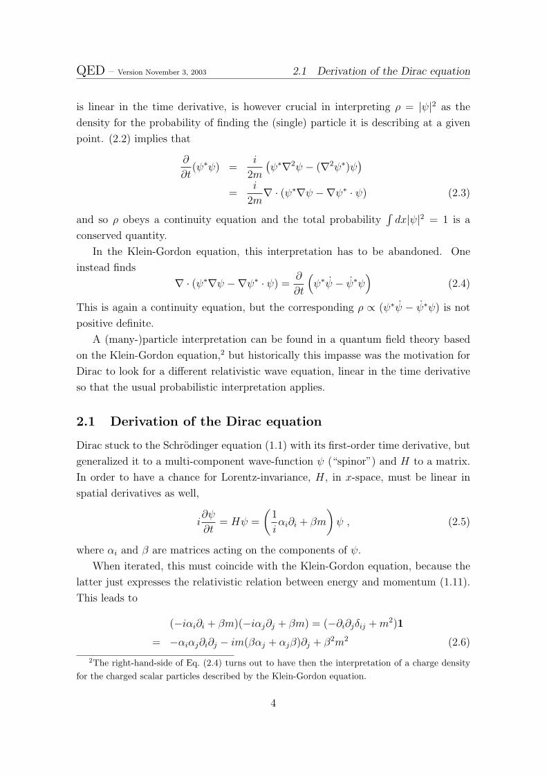
is linear in the time derivative, is however crucial in interpreting ρ = |ψ|2 as the
density for the probability of finding the (single) particle it is describing at a given
point. (2.2) implies that
∂
∂t(ψ∗ψ) =
i
2m
(ψ∗∇2ψ − (∇2ψ∗)ψ
)=
i
2m∇ · (ψ∗∇ψ −∇ψ∗ · ψ) (2.3)
and so ρ obeys a continuity equation and the total probability∫dx|ψ|2 = 1 is a
conserved quantity.
In the Klein-Gordon equation, this interpretation has to be abandoned. One
instead finds
∇ · (ψ∗∇ψ −∇ψ∗ · ψ) =∂
∂t
(ψ∗ψ − ψ∗ψ
)(2.4)
This is again a continuity equation, but the corresponding ρ ∝ (ψ∗ψ − ψ∗ψ) is not
positive definite.
A (many-)particle interpretation can be found in a quantum field theory based
on the Klein-Gordon equation,2 but historically this impasse was the motivation for
Dirac to look for a different relativistic wave equation, linear in the time derivative
so that the usual probabilistic interpretation applies.
2.1 Derivation of the Dirac equation
Dirac stuck to the Schrodinger equation (1.1) with its first-order time derivative, but
generalized it to a multi-component wave-function ψ (“spinor”) and H to a matrix.
In order to have a chance for Lorentz-invariance, H, in x-space, must be linear in
spatial derivatives as well,
i∂ψ
∂t= Hψ =
(1
iαi∂i + βm
)ψ , (2.5)
where αi and β are matrices acting on the components of ψ.
When iterated, this must coincide with the Klein-Gordon equation, because the
latter just expresses the relativistic relation between energy and momentum (1.11).
This leads to
(−iαi∂i + βm)(−iαj∂j + βm) = (−∂i∂jδij +m2)1
= −αiαj∂i∂j − im(βαj + αjβ)∂j + β2m2 (2.6)
2The right-hand-side of Eq. (2.4) turns out to have then the interpretation of a charge densityfor the charged scalar particles described by the Klein-Gordon equation.
4

QED – Version November 3, 2003 2.2 Properties of the Dirac matrices
which requires that
αi, αj = 2δij (2.7)
αi, β = 0 (2.8)
β2 = 1 (2.9)
Because of (2.9), multiplying (2.5) by β gives the Lorentz-covariant form of the
Dirac equation
(iγµ∂µ −m)ψ(x) =: (i /∂ −m)ψ(x) = 0 (2.10)
with the Dirac γ-matrices
γµ = (γ0, γm) = (β, βαm) (2.11)
which satisfy the Clifford algebra relation
γµ, γν = 2gµν1 (2.12)
2.2 Properties of the Dirac matrices
Before giving an explicit representation of the Dirac matrices, let us list their general,
representation-independent properties.
i) Hermiticity of the Hamilton operator H requires Hermiticity of the matrices
~α, β. This implies that γ0 = β is hermitian, (γ0)† = γ0, and that γi is anti-hermitian:
(γi)† = (βαi)† = αiβ = −βαi = −γi .
ii) Because (αi)2 = β2 = 1, the eigenvalues of the matrices αi, β (= γ0) are ±1.
On the other hand, (γi)2 = −1 and the eigenvalues of the γi are ±i.iii) The matrices αi, β, γ
µ are all traceless. This follows from taking the trace of
both sides of
αi = −βαiβ, β = −α(i)βα(i), γi = −γ0γiγ0
(brackets around repeated indices denote exemption from the Einstein summation
convention) and using cyclicity of the trace, i.e. tr(ABC) = tr(BCA).
iv) From ii) and iii) follows that the dimension of the Dirac matrices must be
even.
Among 2-dimensional matrices, one can find just 3 anticommuting, hermitean
matrices with the required properties for αi, β: the Pauli matrices
σ1 =
(0 1
1 0
), σ2 =
(0 −ii 0
), σ3 =
(1 0
0 −1
). (2.13)
5

QED – Version November 3, 2003 2.3 Dirac adjoint and Dirac current
These can be used to write a Dirac equation in up to 2+1 space-time dimensions. In
4 dimensions, the Pauli matrices suffice for (2.5), if we omit the mass term, leading
to the so-called Weyl equation, which however cannot be rewritten into (2.10) with
(2.12), because that would require 4 matrices.
In 3+1 dimensional space-time, the matrix dimension of the γ’s must be ≥ 4.
Indeed, using the Pauli matrices as building blocks, one possibility is the following
(Dirac representation)
αi =
(0 σi
σi 0
), β =
(12 0
0 −12
)= γ0, γi =
(0 σi
−σi 0
). (2.14)
However, this choice is not unique. γµ → UγµU−1 with U unitary (to preserve
the Hermiticity properties) gives an equivalent representation.
Another useful representation is the so-called Weyl or chiral representation
γ0 =
(0 12
12 0
), γi =
(0 σi
−σi 0
). (2.15)
Yet another one is the so-called Majorana representation
γ0 =
(0 σ2
σ2 0
), γ1 =
(iσ3 0
0 iσ3
), γ2 =
(0 −σ2
σ2 0
), γ3 =
(−iσ1 0
0 −iσ1
),
(2.16)
where all γ-matrices are purely imaginary. This implies that (iγµ∂µ − m)ψ = 0
becomes a purely real equation, and that the real and imaginary parts of ψ are
decoupled. As we shall see, this nice feature is lost when ψ is coupled to electromag-
netic fields. Neutral particles on the other hand may well be “Majorana”, meaning
that, in the Majorana representation3, they can be described by a real field ψ, and
thus by half as many degrees of freedom as those of a complex Dirac field. However,
the standard model of elementary particle physics does not (yet) have Majorana
particles.
2.3 Dirac adjoint and Dirac current
Because the Hermiticity properties of the γ-matrices can be summarized by
㵆 = γ0γµγ0 (2.17)
it is natural to define the Dirac adjoint spinor by
ψ := ψ†γ0 (2.18)
3In other representations, a reality condition on ψ is slightly more involved, but of course stillpossible to formulate.
6

QED – Version November 3, 2003 2.4 Covariance of the Dirac equation
Taking the adjoint of the Dirac equation (iγµ∂µ −m)ψ = 0 gives
ψ†(−i㵆←∂µ −m) = 0 ⇒ ψ(i←/∂ +m) = 0. (2.19)
(2.19) together with the original form of the Dirac equation establishes that there is
a conserved current
ψ(←/∂ + /∂→)ψ = ∂µ(ψγµψ︸ ︷︷ ︸jµ
) = 0 (2.20)
with positive definite density
j0 = ρ = ψγ0ψ = ψ†ψ =4∑
α=1
ψ†αψα ≥ 0 . (2.21)
This opens the possibility of interpreting ρ as a probability density in analogy with
the nonrelativistic Schrodinger equation, or in other words to use the Dirac equation
as a single-particle relativistic wave equation. The price to pay is that the Dirac wave
function has 4 components (Dirac spinor), which we shall label by indices from the
beginning of the Greek alphabet. As we shall see presently, a spinor transforms rather
differently from a 4-vector. (That both involve the same number of components is
an accident of 4-dimensional space-time; in n dimensions a Dirac spinor has 2[n/2]
components.)
2.4 Covariance of the Dirac equation
Although we have suggested covariance of the Dirac equation by using a relativistic
notation for the γ-matrices, it remains to show that the Dirac equation is indeed co-
variant under Lorentz transformations, or, more generally, under the Lorentz group
plus translations (Poincare group). This means that the Dirac equation should pre-
serve its form after a transformation to a different frame of reference by an arbitrary
Poincare transformation
x′µ = Lµνxν + aµ, LTgL = g (2.22)
with a well-defined local relation between ψ′(x′) and ψ(x) so that
iγµ∂
∂xµψ(x)−mψ(x) = 0
⇒ iγµ∂
∂x′µψ′(x′)−mψ′(x′) = 0 (2.23)
i) Translations: Because ∂/∂xµ = ∂/∂(x + a)µ = ∂/∂x′µ, these are trivially
realized by ψ′(x′) = ψ(x) or
ψ′(x) = ψ(x− a) (2.24)
7

QED – Version November 3, 2003 2.4 Covariance of the Dirac equation
ii) Lorentz transformations: If we assume a linear relation
ψ′α(x′) = Sαβ(L)ψβ(x), x′µ = Lµνx
ν , (2.25)
form invariance of the Dirac equation, in which
∂
∂x′µ=
∂xν
∂x′µ︸︷︷︸(L−1)ν
µ
∂
∂xν
requires that
S−1γµ(L−1)νµS = γν ⇒ S−1(L)γµS(L) = Lµνγν (2.26)
This fits perfectly to the Clifford relation (2.12) which is left unchanged because
of Lµσ Lνρ g
σρ = gµν .
The existence of a matrix S(L) for all Lorentz transformations L is guaranteed by
the following theorem from group theory:4 The Clifford algebra relation Ai, Aj =
2qij1 with qij a symmetric n × n matrix and n even has precisely one equivalence
class of irreducible representations of dimension 2n/2.
This determines S(L) uniquely up to a factor, which turns out to be ±1; the
S(L) thus form a two-valued representation of the Lorentz group.
For infinitesimal Lorentz transformations, however, the relation L → S(L) is
unique once we require that S(1) = 1. Consider
Lµν = δµν + ε ωµν (2.27)
with infinitesimal ε.
Requiring that (2.27) be a Lorentz transformation (LTgL = g) is equivalent to
ωµν = −ωνµ. There are therefore 6 independent ωµν , matching the number of the
generators of spatial rotations (3) plus those of Lorentz boosts (3).
An ansatz S = 1 + εT , S−1 = 1− εT in (2.26) leads to
[γµ, T ] = ωµνγν (2.28)
and this is solved by (exercise!)
T =1
8ωµν [γ
µ, γν ]. (2.29)
4See e.g. Sexl/Urbantke: Relativitat, Gruppen, Teilchen (Springer Verlag)
8

QED – Version November 3, 2003 2.4 Covariance of the Dirac equation
2.4.1 Example: Rotation about z-axis
An infinitesimal rotation about the z-axis is given by
x′ = x+ εy, y′ = y − εx, z′ = z (2.30)
The corresponding ωµν is given by ω12 = g2νω1ν = −1, ω21 = +1, and all other
components zero. This gives
S = 1 +ε
8ωµν [γ
µ, γν ] = 1− ε
4[γ1, γ2] = 1 + ε
i
2Σ3 (2.31)
with Σ3 = σ3 ⊕ σ3 in the Dirac and in the chiral representation of the γ matrices.
Writing out ψ′(x′) = Sψ(x) gives
ψ′(~x) = (1 + εi
2Σ3)ψ(x− εy, y + εx, z)
= ψ(~x) + iε[ 1
2Σ3︸︷︷︸
Spin sz
+ (x∂
i∂y− y ∂
i∂x)︸ ︷︷ ︸
`z︸ ︷︷ ︸Jz
]ψ(~x) (2.32)
Because Σ3 has eigenvalues ±1, this shows5 that ψ carries spin 12.
Finite rotations with angle ϕ can be obtained as
ψ′(~x′) = limN→∞
(1 +
i
2
ϕ
NΣ3
)Nψ(~x) = expiϕ
2Σ3ψ(~x) (2.33)
and we see that a rotation by ϕ = 2π, which corresponds to L = 1, is mapped to
S = eiπΣ3 = −1. Only a rotation by ϕ = 4π brings us back to S = 1.
This two-valuedness of the spinor representation of the rotation group is inherited
by the full Lorentz group (with all complications coming solely from the rotations).6
5Strictly speaking, the identification of spin sz = 12Σ3 or more generally si = 1
2Σi = i8εijk[γj , γk]
does not make sense relativistically: ~s commutes with the Dirac operator /P only in the rest framePµ = mδ0µ. The proper definition is through the Pauli-Lubanski vector Wµ = − 1
2εµνρσSνρPσ,
which for Pµ = mδ0µ reduces to Wµ = (0,m~s). [εµνρσ is the totally antisymmetric ε-tensor withε0123 = +1 = −ε0123.]
6In group theory language: the spinor representation is a one-valued representation of the groupSU(2), which is the universal (2:1) covering group of SO(3). The covering group of the (componentof unity) of the Lorentz group SO0(3,1)⊃SO(3) is the group SL(2,C)⊃SU(2). For more details seeSexl/Urbantke: Relativitat, Gruppen, Teilchen (Springer Verlag).
9

QED – Version November 3, 2003 2.4 Covariance of the Dirac equation
2.4.2 Example: Lorentz boost along x-axis
A Lorentz boost along x axis is generated by ω01 = ω1
0 = 1. Because (ωµν)2 =
12 ⊕ 02, and therefore (ωµν)3 = ωµν we find for Lµν = exp (ξωµν)
L =∞∑n=0
ωnξn
n!=∞∑n=0
ω2n︸︷︷︸ω2
∀n>0
ξ2n
(2n)!+∞∑n=0
ω2n+1︸ ︷︷ ︸ω∀n
ξ2n+1
(2n+ 1)!
= 1− ω2 + ω2 cosh ξ + ω sinh ξ (2.34)
Explicitly,
Lµν =
cosh ξ sinh ξ 0 0
sinh ξ cosh ξ 0 0
0 0 1 0
0 0 0 1
(2.35)
which can be identified with (1.6) through β = v = tanh ξ. Indeed, cosh ξ =
1/√
1− β2 = γ, and sinh ξ = βγ. The parameter ξ is called rapidity ; it is par-
ticularly useful because it is additive under successive boosts.
The corresponding spinor transformation S(L) is given by
S(L) = exp
(1
8ξωµν [γ
µ, γν ]
)= exp
(1
4ξ[γ0, γ1]
). (2.36)
In the Dirac representation (2.14), [γ0, γ1] = 2
(0 σ1
σ1 0
)= 2α1. Because (α1)
2 =
14, (α1)3 = α1, etc., we obtain
S(L) = 1 coshξ
2︸ ︷︷ ︸=:C
+α1 sinhξ
2︸ ︷︷ ︸=:S
=
C 0 0 S
0 C S 0
0 S C 0
S 0 0 C
(2.37)
This expression is admittedly not too illuminating, but we shall use this result
later. We shall also find it useful to express ξ in terms of E and px: With v = px
E=
tanh ξ we get
tanhξ
2=
tanh ξ
1 +√
1− tanh2 ξ=
v
1 +√
1− v2=
p
E +m(2.38)
⇒ coshξ
2=
√E +m
2m, sinh
ξ
2= tanh
ξ
2cosh
ξ
2(2.39)
10

QED – Version November 3, 2003 2.4 Covariance of the Dirac equation
2.4.3 Components of the Lorentz group
The finite Lorentz transformation (2.34) and generally any Lorentz transformation
of the form Lµν = exp (ξωµν) is one that is continuously connected with the identity
through the parameter ξ. This does not exhaust all elements of the Lorentz group,
but only those with determinant det(L) = +1 and L00 ≥ 1, for it is not possible by a
continuous change of parameters to jump from these values to the other possibilities
det(L) = −1 and/or L00 ≤ −1. The subgroup of Lorentz transformations with
det(L) = +1 and L00 ≥ 1 is called the proper orthochronous Lorentz group L↑+.
As long as only elements from L↑+ are considered, the representation S(L) of
the Lorentz group7 is reducible (i.e.: there are nontrivial invariant subspaces). This
becomes manifest in the chiral representation of the Dirac matrices (2.15), in which
the generators of
S(L) = exp
(− i
2ωµνS
µν
), L ∈ L↑+ (2.40)
(where the parameter ξ is now implicit in ωµν) read
S0i =i
4[γ0, γi] = − i
2
(σi 0
0 −σi
), Sij =
i
4[γi, γj] =
1
2εijk
(σk 0
0 σk
). (2.41)
The upper two and lower two components of a four-component spinor therefore
transform without being mixed.
It is in fact possible to write a relativistic wave equation for a spinor which has
only half of the components of a Dirac spinor: when the mass is put to zero, the
Dirac equation (in the chiral representation) also does not mix the upper and lower
half of a spinor. Putting to zero one half, ψ =(φ0
), or ψ =
(0χ
)leads to the so-called
Weyl equation (p0 + ~p · ~σ
)φ = 0 or
(p0 − ~p · ~σ
)χ = 0 (2.42)
which is of great importance in the theory of weak interactions, where it describes
massless neutrinos.
The full Lorentz group is obtained by composing elements of L↑+ with the discrete
operations of space inversion P or time reversal T or both together.
Space inversion (“parity transformation”) is effected by
Lµν =
(1
−13
)and so this must be represented by a matrix S(L) = P with the properties
γ0 = P−1γ0P, ~γ = −P−1~γP. (2.43)
7More precisely: the covering group of L↑+
11

QED – Version November 3, 2003 2.4 Covariance of the Dirac equation
This is solved by P = ±γ0. In the chiral representation (2.15), γ0 is block-off-
diagonal, so the upper and lower halves of a spinor no longer define invariant sub-
spaces if parity is included. A Weyl spinor which involves only one half therefore
breaks parity, and indeed parity has been found to be violated in weak interactions.
The Dirac equation on the other hand is parity invariant and so is quantum electro-
dynamics.
Space inversion together with time reversal, PT, is effected by Lµν = −δµν , and
so
γµ = −S(PT )−1γµS(PT ) (2.44)
One easily verifies that a solution for S(PT ) is
γ5 := iγ0γ1γ2γ3 ≡ i
4!εµνρσγ
µγνγργσ (2.45)
γ5 has the properties
γ5 = (γ5)†, (2.46)
(γ5)2 = 1, (2.47)
γ5, γµ = 0 (2.48)
The last relation (2.48) implies that [γ5, Sµν ] = 0, which again proves, by Schur’s
lemma8, that S(L ∈ L↑+) = exp(− i2ωµνS
µν) is reducible. The invariant subspaces
under the latter transformations are given by the two projection operators
PL =1
2(1− γ5), PR =
1
2(1 + γ5) (2.49)
which project onto left- and right-handed chiralities, respectively.
ψL = PLψ and ψR = PRψ are eigenstates of γ5 with eigenvalues +1 and -1,
respectively. Dirac spinors which are solutions of the Dirac equation can have definite
chiralities only in the massless case. By acting with γ5γ0 on /pψ = 0 one can readily
show that (exercise!)~Σ · ~pψ = γ5p0ψ (2.50)
so that with p0 = E = |~p|
1
2γ5ψ =
1
2
~Σ · ~p|~p|
ψ =~s · ~p|~p|
ψ (2.51)
8If a matrix commutes with all elements of a matrix representation of a group, then either it isproportional to the unit matrix or this representation is reducible.
12

QED – Version November 3, 2003 2.4 Covariance of the Dirac equation
Chirality defined as 12
times the eigenvalue of γ5 thus equals the helicity (the
projection of spin on the direction of ~p) of massless particles. This is a boost-
invariant quantity, because massless particles cannot be overtaken. It does however
change under parity.
In the chiral representation (2.15)
γ5chiral rep. =
(−1 0
0 1
)(2.52)
and so the upper (lower) half of a Dirac spinor is of left (right) chirality. As we saw in
(2.41), they transform under different, namely complex conjugated, representations
of L↑+, sometimes denoted as (12, 0) and (0, 1
2), respectively.
In other representations, notably in the Dirac representation (2.14) where
γ5Dirac rep. =
(0 1
1 0
)(2.53)
the above reducibility (when parity is excluded) is less conspicuous.
2.4.4 Dirac field bilinears
The advantage of the Dirac representation is instead in the diagonal form of γ0, which
(besides representing parity) is of singular importance because it effects Hermitian
conjugation of the γ matrices as we have seen in (2.17) and so enters the definition
of Dirac adjoints (2.18).
We still have to establish the transformation properties of the Dirac adjoint in
order to verify covariance of the conserved current (2.20).
Under a Lorentz transformation ψ → S(L)ψ, and so ψ → ψ†S†γ0 = ψγ0S†γ0.
With (2.17) and the explicit form of the S(L) in (2.40) as well as of the S(L) asso-
ciated with parity one can show that (exercise!)
γ0S†γ0 = S−1. (2.54)
Therefore (under orthochronous Lorentz transformations9) ψψ → ψS−1Sψ = ψψ
is a scalar and ψγµψ → ψS−1γµSψ = Lµνψγνψ a vector, as is necessary for the
conserved current (2.20) to make sense.
More generally, ψγµ1 · · · γµkψ transforms as a tensor of rank k. Inserting addi-
tionally the matrix γ5 does not change that as long as we consider Lorentz transfor-
mations L ∈ L↑+, because [γ5, Sµν ] = 0. But under the parity transformation we pick
9We exclude time reversal here, which would lead to a change of sign of ψψ. In the full quantumfield theory, ψψ is made invariant by representing time reversal by an anti-linear transformation.
13
QED – Version November 3, 2003 2.5 Higher spin
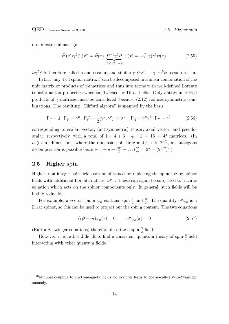
up an extra minus sign:
ψ′(x′)γ5ψ′(x′) = ψ(x) P−1γ5P︸ ︷︷ ︸γ0γ5γ0=−γ5
ψ(x) = −ψ(x)γ5ψ(x). (2.55)
ψγ5ψ is therefore called pseudo-scalar, and similarly ψγµ1 · · · γµkγ5ψ pseudo-tensor.
In fact, any 4×4 spinor matrix Γ can be decomposed in a linear combination of the
unit matrix or products of γ-matrices and thus into terms with well-defined Lorentz
transformation properties when sandwiched by Dirac fields. Only antisymmetrized
products of γ-matrices must be considered, because (2.12) reduces symmetric com-
binations. The resulting “Clifford algebra” is spanned by the basis
ΓS = 1, ΓµV = γµ, ΓµνT =i
2[γµ, γν ] =: σµν , ΓµA = γµγ5, ΓP = γ5 (2.56)
corresponding to scalar, vector, (antisymmetric) tensor, axial vector, and pseudo-
scalar, respectively, with a total of 1 + 4 + 6 + 4 + 1 = 16 = 42 matrices. (In
n (even) dimensions, where the dimension of Dirac matrices is 2n/2, an analogous
decomposition is possible because 1 + n+(n2
)+ . . .
(nn
)= 2n = (2n/2)2.)
2.5 Higher spin
Higher, non-integer spin fields can be obtained by replacing the spinor ψ by spinor
fields with additional Lorentz indices, ψµ.... These can again be subjected to a Dirac
equation which acts on the spinor components only. In general, such fields will be
highly reducible.
For example, a vector-spinor ψµ contains spin 12
and 32. The quantity γµψµ is a
Dirac spinor, so this can be used to project out the spin 12
content. The two equations
(i /∂ −m)ψµ(x) = 0, γµψµ(x) = 0 (2.57)
(Rarita-Schwinger equations) therefore describe a spin-32
field.
However, it is rather difficult to find a consistent quantum theory of spin-32
field
interacting with other quantum fields.10
10Minimal coupling to electromagnetic fields for example leads to the so-called Velo-Zwanzigeranomaly.
14

QED – Version November 3, 2003
3 Solutions of the Dirac equation
3.1 Plane-wave solutions
The simplest solution of the Klein-Gordon equation are plane waves e∓ikµxµwith
k2 = m2, where for k0 > 0 the minus sign corresponds to positive energy (E = i∂t).
For plane-wave solutions of the Dirac equation we make the ansatz
ψ(+)α (x) = e−ik·xuα(k), ψ(−)
α (x) = e+ik·xvα(k) (3.1)
and obtain from (i /∂ −m)ψ(±) = 0 the algebraic equations
( /k −m)u(k) = 0, ( /k +m)v(k) = 0 . (3.2)
Hermitian conjugation and use of (2.17) shows that the corresponding Dirac
adjoints obey similarly
u(k)( /k −m) = 0, v(k)( /k +m) = 0 . (3.3)
In the rest frame kµ = (m,~0), and we have
(γ0 − 1)u(m,~0) = 0, (γ0 + 1)v(m,~0) = 0. (3.4)
In the Dirac representation (2.14), γ0 =
(12 0
0 −12
), so any spinor
(ϕ0
)with
only upper components is a solution for u; conversely, any spinor of the form(
0χ
)is
a solution for the negative-energy case v. A basis is given by
u(1)(m,~0) =
1
0
0
0
, u(2)(m,~0) =
0
1
0
0
, v(1)(m,~0) =
0
0
1
0
, v(2)(m,~0) =
0
0
0
1
,
(3.5)
which moreover gives the eigenvectors of the spin operator 12Σ3 = 1
2σ3 ⊕ σ3 with
eigenvalues +12,−1
2,+1
2,−1
2, respectively.
Note that in other representations of the Dirac matrices, the above unit spinors
would have a different interpretation. For example, in the chiral representation (2.15)
the rest-frame spinors with positive and negative energy have the form u =(ϕϕ
),
v =(χ−χ
).
Solutions for ~k 6= 0 can be obtained by a Lorentz transformation which subjects
u and v to a linear transformation with the matrix S(L). For Lorentz boosts in x-
direction we have calculated S(L) in the Dirac representation in the previous section.
15
QED – Version November 3, 2003 3.2 Klein’s paradox
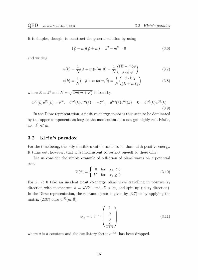
It is simpler, though, to construct the general solution by using
( /k −m)( /k +m) = k2 −m2 = 0 (3.6)
and writing
u(k) =1
N( /k +m)u(m,~0) =
1
N
((E +m)ϕ
~σ · ~k ϕ
)(3.7)
v(k) =1
N(− /k +m)v(m,~0) =
1
N
(~σ · ~k χ
(E +m)χ
)(3.8)
where E ≡ k0 and N =√
2m(m+ E) is fixed by
u(a)(k)u(b)(k) = δab, v(a)(k)v(b)(k) = −δab, u(a)(k)v(b)(k) = 0 = v(a)(k)u(b)(k)
(3.9)
In the Dirac representation, a positive-energy spinor is thus seen to be dominated
by the upper components as long as the momentum does not get highly relativistic,
i.e. |~k| m.
3.2 Klein’s paradox
For the time being, the only sensible solutions seem to be those with positive energy.
It turns out, however, that it is inconsistent to restrict oneself to these only.
Let us consider the simple example of reflection of plane waves on a potential
step
V (~x) =
0 for x1 < 0
V for x1 ≥ 0(3.10)
For x1 < 0 take an incident positive-energy plane wave travelling in positive x1
direction with momentum k =√E2 −m2, E > m, and spin up (in x3 direction).
In the Dirac representation, the relevant spinor is given by (3.7) or by applying the
matrix (2.37) onto u(1)(m,~0),
ψin = a eikx1
1
0
0k
E+m
(3.11)
where a is a constant and the oscillatory factor e−iEt has been dropped.
16

QED – Version November 3, 2003 3.2 Klein’s paradox
For the reflected wave we make the ansatz of plane waves travelling in negative
x1 direction with a superposition of spin up and spin down,
ψrefl = b e−ikx1
1
0
0−kE+m
+ b′ e−ikx1
0
1−kE+m
0
, (3.12)
and similarly for the transmitted wave
ψtrans = d eik′x1
1
0
0k′
E−V+m
+ d′ eik′x1
0
1k′
E−V+m
0
, (3.13)
but with k′ =√
(E − V )2 −m2.
Continuity requires that ψin + ψrefl
∣∣∣x1=0
= ψtrans
∣∣∣x1=0
. This gives b′ = d′ = 0 (i.e.
no spin flips) and
b
a=
1− ρ1 + ρ
,d
a=
2
1 + ρ, ρ :=
k′
k
E +m
E − V +m. (3.14)
As long as E −m > V , there is partial reflection and partial transmission with
reflection and transmission coefficients
R =jrefljin
=
(b
a
)2
=
(1− ρ1 + ρ
)2
, T =jtrans
jin= 1− jrefl
jin=
4ρ
(1 + ρ)2(3.15)
with R→ 1 and T → 0 as the barrier is increased to V → E −m.
When V > E −m, k′ becomes imaginary and there is exponential decay with a
penetration length
d = 1/√m2 − (V − E)2. (3.16)
However, something very strange happens when V is increased further and fur-
ther. First, the penetration length decreases as one would expect. But obviously,
there is a minimum at d = 1/m, the Compton wavelength (≈ 4 × 10⁻¹³m for elec-
trons), which is reached when V − (E − m) = m. Increasing V still further no
longer restricts the penetration region but makes it larger again. Even weirder,
when V − (E −m) > 2m, k′ becomes real again, and ψtrans oscillatory. In this case,
ρ < 0, and therefore jtrans < 0 and jrefl > jin.
This is Klein’s paradox. It shows that the Dirac equation can be interpreted as a
single-particle theory only as long as there are no external forces and energies which
are comparable to the mass scale m.
17

QED – Version November 3, 2003 3.2 Klein’s paradox
Although the above example is rather artificial, it points to phenomena such as
pair creation in strong fields. It also indicates that in a relativistic theory there
is, besides the well-known uncertainty principle, a fundamental lower limit to the
localizability of a single particle, which is given by its Compton wavelength.
Let us confirm this latter statement by an attempt to construct a localized wave
packet. At time t = 0 we take
ψ(0, ~x) = e−~x2/(2D2)w (3.17)
with a fixed spinor w =(ϕ0
).
The general solution of the free Dirac equation is given by a superposition of the
plane waves obtained in the preceding section,
ψ(t, ~x) =
∫d3p
(2π)3
m
E
2∑a=1
b(p; a)u(a)(p)e−ip·x + d∗(p; a) v(a)(p)eip·x
(3.18)
where b and d∗ are the expansion coefficients of positive and negative-energy solutions
(the factor m/E is introduced for convenience only). These are determined by the
initial condition (3.17) through∫d3xe−i~p~xψ(0, ~x) = (2πD2)3/2e−~p
2D2/2w =m
E
2∑a=1
b(p; a)u(a)(p) + d∗(p; a) v(a)(p)
(3.19)
where p := (p0,−~p).As one easily verifies from the explicit expressions (3.7) and (3.8), the following
orthogonality relations hold
u†(a)(k)u(b)(k) =E
mδab = v†(a)(k)v(b)(k),
v†(a)(k)u(b)(k) = 0 = u†(a)(k)v(b)(k). (3.20)
These we can use to calculate
b(p; a) = (2πD2)3/2e−~p2D2/2 u†(a)(p)w
d∗(p; a) = (2πD2)3/2e−~p2D2/2 v†(a)(p)w. (3.21)
From (3.7) and (3.8) we see that the ratio of the amplitudes of negative-energy
solutions over positive-energy ones is of the order of d∗/b ∼ |~p|/(E + m). As long
as D is much larger than the Compton wavelength, D 1/m, there are essential
contributions only from |~p| m, and thus d∗/b 1. However, if one tries to localise
18

QED – Version November 3, 2003 3.3 Electromagnetic coupling
the wavefunction to be comparable or smaller than the Compton wavelength, the
negative-energy solutions become important and can no longer be neglected.
The presence of non-negligible negative-energy solutions has a curious conse-
quence for the behaviour of the current density ~j = ψ~γψ. While this current equals
〈~p/E〉 (the group velocity of the wave packet) so long as there is only a positive-energy
component, with both components there is also an interference term involving e2iEt.
Because E ≥ m, this introduces an oscillatory contribution with extremely high
frequencies ≥ 2m ≈ 2× 10²¹Hz called “zitterbewegung”.
Despite these limitations, the Dirac equation used as a generalization of the
Schrodinger equation is of great importance and we shall elaborate on it further
before setting up the full quantum field theory, bearing in mind however that a
single (or fixed-number) particle theory makes sense only as long as all energies
involved are well below the particles’ rest mass and therefore all length scales are
much larger than the Compton wavelength.
3.3 Electromagnetic coupling
We begin by recapitulating the relativistic form of Maxwell’s equations, using units
where c = 1 and the Coulomb force between charges is Q1Q2/4πr (Heaviside units).
The electric and magnetic fields are part of an antisymmetric tensor
F µν = −F νµ =
0 −E1 −E2 −E3
E1 0 −B3 B2
E2 B3 0 −B1
E3 −B2 B1 0
. (3.22)
Combining the electric charge and current in
jµ = (ρ,~j) (3.23)
one half of Maxwell’s equation, namely,
div ~E = ρ, rot ~B − ∂t ~E = ~j (3.24)
can be written covariantly as
∂µFµν = jν (3.25)
and the other half
div ~B = 0, rot ~E + ∂t ~B = 0 (3.26)
19

QED – Version November 3, 2003 3.3 Electromagnetic coupling
in terms of the “dual” field strength tensor F µν := 12εµνσρFσρ as
∂µFµν = 0. (3.27)
F is obtained from (3.22) by substituting ~E → − ~B and ~B → ~E, so (3.27) expresses
the absence of magnetic sources. The totally antisymmetric tensor εµνσρ equals +1
(-1) for (µ, ν, σ, ρ) an even (odd) permutation of (0,1,2,3). Note that ε0123 = −ε0123.
The second set of Maxwell’s equations (3.27) can be solved by writing
F µν = ∂µAν − ∂νAµ, Aµ = (φ, ~A) (3.28)
where the 4-potential Aµ is determined only up to local gauge transformations δAµ =
∂µΛ(x) which leave F µν invariant.
The source-containing set of Maxwell’s equations (3.25) are compatible with the
antisymmetry of F µν only if j is a conserved current: ∂νjν = ∂ν∂µF
µν ≡ 0.
In the Dirac theory, jµ = eψγµψ is a suitable candidate for the electromagnetic
current. Conversely, the Dirac field can be coupled to the electromagnetic field by
the “minimal” substitution ∂µ → ∂µ + ieAµ, leading to
(i /∂ − e /A(x)−m)ψ(x) = 0. (3.29)
The arbitrariness of the gauge potential A due to gauge transformations Aµ(x) →Aµ(x) + ∂µΛ(x) can be compensated by a local phase rotation ψ(x)→ e−ieΛ(x)ψ(x).
The latter shows that electrodynamics is associated with the (Abelian) gauge group
U(1) — unitary matrices with dimension 1. It is the simplest example of the more
general class of Yang-Mills theories, where Λ becomes a nontrivial matrix built from
the generators of some generally nonabelian group.
Writing (3.29) in terms of the ~α and β matrices we have
i∂ψ
∂t= (~α · ~p+ βm)︸ ︷︷ ︸
H0
ψ +(−e~α · ~A+ eφ
)︸ ︷︷ ︸
Hint
ψ. (3.30)
This resembles the interaction of a classical particle in an external field with ~α playing
the role of velocity. Indeed, we have ~x = i[H,~x] = ~α.
To study the physical content of the Dirac equation coupled to electromagnetic
fields we shall first consider its nonrelativistic limit.
3.3.1 Nonrelativistic limit
In the limit of E−m m, it is appropriate to separate off the large energy associated
with the particle’s rest mass and to write
ψ(t, ~x) = e−imt(ϕ(t, ~x)
χ(t, ~x)
). (3.31)
20

QED – Version November 3, 2003 3.3 Electromagnetic coupling
In the standard Dirac representation (2.14), this gives
i∂ϕ
∂t= ~σ · (~p− e ~A) χ+ eA0 ϕ (3.32)
i∂χ
∂t= ~σ · (~p− e ~A) ϕ+ eA0 χ− 2mχ (3.33)
The latter equation is dominated by the mass term, against which iχ can be neglected
in the nonrelativistic limit, so this equation can be solved algebraically. Assuming
further that eA0 m, we have
χ ≈ 1
2m~σ · (~p− e ~A)ϕ ϕ. (3.34)
The Dirac spinor is thus seen to be separated in large and small components ϕ and
χ, with ϕ being determined by the so-called Pauli equation obtained by inserting
(3.34) into (3.32),
i∂ϕ
∂t=
[1
2m(~σ · ~π)2 + eA0
]ϕ, ~π := ~p− e ~A(x). (3.35)
Because σiσj = 12σi, σj+ 1
2[σi, σj] = δij + iεijkσk we can rewrite this according to
(~σ · ~π)2 = ~π2 +i
2εijkσk[πi, πj] = ~π2 − e εijk∂iAj︸ ︷︷ ︸
Bk
σk (3.36)
yielding the alternative version
i∂ϕ
∂t=
[1
2m
(~p− e ~A
)2
+ eA0 − e
2m~σ · ~B
]ϕ . (3.37)
In the special case of a weak constant magnetic field, ~A = 12~B × ~x, one has
(~p − e ~A)2 ≈ ~p2 − e (~x × ~p) · ~B and the operator on the right-hand-side of the Pauli
equation becomes
HPauli ≈~p2
2m+ eA0 − e
2m︸︷︷︸µB
(~L+ 2~S
)· ~B, ~S ≡ 1
2~σ . (3.38)
The magnetic moment associated with spin is thus seen to have an anomalous fac-
tor of 2. This gyromagnetic ratio g = (|magnetic moment|× |spin|)/(Bohr magneton
µB) = 2 is our first nontrivial prediction of the Dirac theory, and it is indeed in good
agreement with the actual magnetic moment of electrons and muons11; the small
deviations from g = 2 that are observed experimentally will find their explanation
in the full quantum electrodynamics.
11The gyromagnetic ratio for protons and neutrons is however substantially different from 2,pointing to their important internal structure.
21

QED – Version November 3, 2003 3.4 Foldy-Wouthuysen transformation
In the relativistic Dirac equation, the spin-dependent interactions can be isolated
by acting on (3.29) with (i /∂ − e /A+m). In analogy to the steps leading from (3.35)
to (3.37) one obtains[(i /∂ − e /A)2 −m2
]ψ =
[(i∂ − eA)2 −m2 − e
2σµνFµν
]ψ = 0, σµν :=
i
2[γµ, γν ]
(3.39)
with 12~σµνFµν = (i~α · ~E + ~Σ · ~B).
3.4 Foldy-Wouthuysen transformation
By decoupling large and small components of a Dirac spinor in the nonrelativistic
approximation we have been able to highlight some of its physical content. Such a
procedure can be carried out systematically in a series expansion in powers of Ekin/m
and has been worked out by Foldy and Wouthuysen (1950).
The goal is to find a unitary transformation
ψ′ = eiSψ (3.40)
for ψ of (3.30) such that in
i∂tψ′ = eiS
(He−iS − i(∂te−iS)
)ψ′ =: H ′ψ′ (3.41)
H ′ takes a block-diagonal form, at least up to some order of a nonrelativistic expan-
sion.
A familiar similar problem is the diagonalization of a Hamilton operator H =
σxBx+σzBz. This is achieved by a rotation about the y-axis by ei2σyθ = e
12σzσxθ with
tan θ = Bx/Bz.
3.4.1 Free Dirac equation
In the case of the free Dirac equation where H = ~α · ~p + βm with α and β as given
in the Dirac representation (2.14), we have a similar structure with σx ↔ ~α · ~p and
β ↔ σz. This motivates an ansatz of the form
eiS = exp (β~α · ~pθ(p)/|~p|) = exp
(1
|~p|~γ · ~pθ(p)
). (3.42)
Because(~γ·~p|~p|
)2
= −1, we can easily calculate
eiS = cos θ +~γ · ~p|~p|
sin θ (3.43)
22

QED – Version November 3, 2003 3.4 Foldy-Wouthuysen transformation
and
H ′ = eiSHe−iS =
(cos θ + β
~α · ~p|~p|
sin θ
)(~α · ~p+ βm)
(cos θ − β ~α · ~p
|~p|sin θ
)= (~α · ~p+ βm)
(cos θ − β ~α · ~p
|~p|sin θ
)2
︸ ︷︷ ︸exp(−2β ~α·~p
|~p| θ)
= (~α · ~p+ βm)
(cos 2θ − β ~α · ~p
|~p|sin 2θ
)
= ~α · ~p[cos 2θ − m
|~p|sin 2θ
]+ β
[m cos 2θ +
~p2
|~p|sin 2θ
](3.44)
In order that H ′ becomes diagonal, the first of the square brackets has to vanish.
This leads to tan 2θ = |~p|m
, which entails sin 2θ = |~p|E
, cos 2θ = mE
, for E ≡√~p2 +m2,
and so
H ′ = β√~p2 +m2 =
(√~p2 +m212 0
0 −√~p2 +m212
)(3.45)
We have therefore managed to diagonalize the Dirac Hamitonian, which clearly dis-
plays the solutions corresponding to positive and negative energies.
Note however that the transformation leading to (3.45) is nonlocal. In configura-
tion space, the FW-transformed spinor (3.40) would have to be written as a nontrivial
integral∫dx′〈x|eiS|x′〉ψ(x′) over all of 3-space, where the main contribution comes
from a neighbourhood of x with radius 1/m. Also, the usual ~x-operator changes its
meaning when applied directly to ψ′. As such it is referred to as “mean location”.
Transformed back into the standard formulation it corresponds to the nonlocal op-
erator ~xmean = e−iS~xeiS. If one defines similarly a mean angular momentum and a
mean spin operator, these are found to commute with the free Hamilton operator,
in constrast to the usual local quantities.
3.4.2 Interacting Dirac equation
When external fields are present, eiS will have to depend explicitly on space and
time12 as well. This makes a solution in closed form impossible in general and one
has to be content with an approximate solution. We shall consider a nonrelativistic
expansion, where |~p|/m, | ~A|/m, and |A0|/m are supposed to be small parameters.
The interaction Hamiltonian
H = βm+O + E ≡ βm+ (~α · (~p− e ~A)) + eA01 (3.46)
is dominated by the block-diagonal mass term. The aim is to get rid of the off-
diagonal (“odd”) term O.
12A time dependence moreover leads to a shift of the energy eigenvalues.
23

QED – Version November 3, 2003 3.4 Foldy-Wouthuysen transformation
In the free case, this was achieved by iS = βOfreeθ(p)/|~p| with θ = 12arctan(|~p|/m).
For |~p|/m 1 we can approximate θ ≈ |~p|/2m.
As a first step, we can try eiS = e1
2mβO. This gives H ′ = βm + O′ + E ′ where
O′ = O( 1m
). This procedure can now be repeated with eiS′= e
12m
βO′and so forth,
successively increasing the order of the odd terms.
After 3 iterations, one finds13 in terms of “mean” operators
H ′′′ = βm+ E ′′′ +O(1
m3)
= β
[m+
(~p− e ~A)2
2m− ~p4
8m3
]+ eφ− e
2mβ~σ · ~B (3.47)
+(−i e
8m2~σ · rot ~E − e
4m2~σ · ( ~E × ~p)
)(3.48)
− e
8m2~∇ · ~E (3.49)
The first terms (3.47) are what we have found in the Pauli equation (3.37) except
that there is now a relativistic correction term to the kinetic energy.
The terms (3.48) contain spin-orbit interactions. With ~p ≈ m~v, the latter of the
two reads
−1
2
e
2m~σ · ( ~E × ~v).
( ~E × ~v) is the magnetic field as seen from a particle moving with velocity ~v through
the electric field ~E, −e2m
is the usual coefficient of the magnetic dipol energy as in
(3.47), and the extra factor 12
can be understood as the effect of Thomas precession,
which happens to reduce the gyromagnetic factor g = 2 to the standard value 1.
In a static, spherically symmetric potential, rot ~E = 0 and the spin-orbit terms
(3.48) reduce toe
4m2r
dφ
dr~L · ~σ.
The last term (3.49) is called Darwin term. It can be interpreted as arising from
fluctuations of the position of an electron ~x with 〈δ~x〉 = 0 but 〈(δ~x)2〉 > 0, which
entails a shift of the electrostatic energy according to
e〈φ(~x+ δ~x)〉 = eφ(~x) +e
2
∂2φ
∂xi∂xj〈δxiδxj〉︸ ︷︷ ︸13δij〈(δ~x)2〉
= eφ(~x) +e
64φ︸︷︷︸−div ~E
〈(δ~x)2〉 (3.50)
The fundamental uncertainty of position that we have observed before (zitterbewe-
gung) was of the order of the Compton wavelength, so we expect 〈(δ~x)2〉 ∼ 1/m2.
So (3.50) is consistent in sign and order of magnitude with the Darwin term (3.49).
13See e.g. Bjorken/Drell: Relativistic quantum mechanics, ch. 4.
24

QED – Version November 3, 2003 3.5 Hydrogen-like atoms
3.5 Hydrogen-like atoms
3.5.1 Spinor harmonics
The free Hamilton operator H0 = ~α · ~p + βm commutes with the total angular
momentum ~J = ~L+ ~S, ~S = 12~Σ, but not separately with ~L or ~S. The same holds true
in a spherical symmetric electrostatic potential, because [~L, f(r)] = 0 = [~Σ, f(r)],
H = ~α · ~p+ βm+ eA0(r), [H, ~J ] = 0. (3.51)
Intuitively, one might expect that if not all of ~S then at least ~S · ~J should be
conserved, which would be the case for a spin in precession around the conserved
total angular momentum. However, one finds
[H, ~Σ · ~J ] = [H, ~Σ] · ~J = 2i(~α× ~p) · ~J. (3.52)
As a second guess, let us try β~Σ · ~J
[H, β~Σ · ~J ] = [H, β]︸ ︷︷ ︸−2β~α·~p
~Σ · ~J + β [H, ~Σ] · ~J (3.53)
This can be streamlined by using that ~α = γ5~Σ and rewriting
~α · ~p ~Σ · ~J = γ5 ~Σ · ~p ~Σ · ~J = γ5~p · ~J + i(~α× ~p) · ~J (3.54)
which shows that
[H, β~Σ · ~J ] = −2βγ5~p · ~J = −βγ5~p · ~Σ = −β~p · ~α =1
2[H, β]. (3.55)
Hence,
[H, β(~Σ · ~J − 1
2)] =: [H,K] = 0, (3.56)
so the “spin-orbit” operator K defines a further conserved quantity. Using that
(~Σ)2 = 3, it can be alternatively expressed as
K = β(~Σ · ~J − 1
2) = β(~Σ · ~L+ 1) = β( ~J2 − ~L2 +
1
4). (3.57)
In the standard Dirac representation where ~Σ = ~σ ⊕ ~σ, this is a block-diagonal
operator with just a different sign in the upper and lower blocks. We can therefore
construct eigenstates of ~J2, Jz, and K out of 2-component spinors ϕ which are
eigenstates of ~J2, Jz, and (~σ · ~L+ 1). The eigenvalues of the latter are
k = j(j + 1)− l(l + 1) +1
4.
25
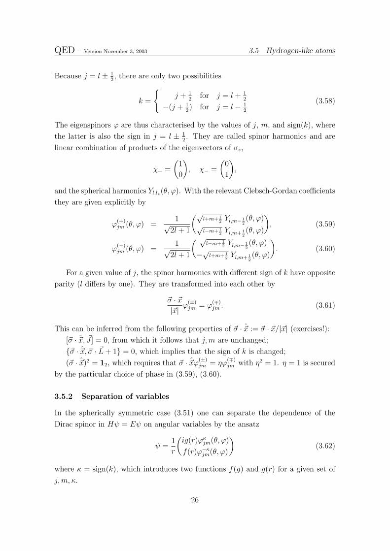
QED – Version November 3, 2003 3.5 Hydrogen-like atoms
Because j = l ± 12, there are only two possibilities
k =
j + 1
2for j = l + 1
2
−(j + 12) for j = l − 1
2
(3.58)
The eigenspinors ϕ are thus characterised by the values of j, m, and sign(k), where
the latter is also the sign in j = l ± 12. They are called spinor harmonics and are
linear combination of products of the eigenvectors of σz,
χ+ =
(1
0
), χ− =
(0
1
),
and the spherical harmonics Yl,lz(θ, ϕ). With the relevant Clebsch-Gordan coefficients
they are given explicitly by
ϕ(+)jm (θ, ϕ) =
1√2l + 1
(√l+m+ 1
2Yl,m− 1
2(θ, ϕ)
√l−m+ 1
2Yl,m+ 1
2(θ, ϕ)
), (3.59)
ϕ(−)jm (θ, ϕ) =
1√2l + 1
( √l−m+ 1
2Yl,m− 1
2(θ, ϕ)
−√l+m+ 12Yl,m+ 1
2(θ, ϕ)
). (3.60)
For a given value of j, the spinor harmonics with different sign of k have opposite
parity (l differs by one). They are transformed into each other by
~σ · ~x|~x|
ϕ(±)jm = ϕ
(∓)jm . (3.61)
This can be inferred from the following properties of ~σ · ~x := ~σ · ~x/|~x| (exercises!):
[~σ · ~x, ~J ] = 0, from which it follows that j,m are unchanged;
~σ · ~x, ~σ · ~L+ 1 = 0, which implies that the sign of k is changed;
(~σ · ~x)2 = 12, which requires that ~σ · ~xϕ(±)jm = ηϕ
(∓)jm with η2 = 1. η = 1 is secured
by the particular choice of phase in (3.59), (3.60).
3.5.2 Separation of variables
In the spherically symmetric case (3.51) one can separate the dependence of the
Dirac spinor in Hψ = Eψ on angular variables by the ansatz
ψ =1
r
(ig(r)ϕκjm(θ, ϕ)
f(r)ϕ−κjm(θ, ϕ)
)(3.62)
where κ = sign(k), which introduces two functions f(g) and g(r) for a given set of
j,m, κ.
26

QED – Version November 3, 2003 3.5 Hydrogen-like atoms
This gives
(E −m− eA0)ig
rϕκjm = ~σ · ~p f
rϕ−κjm (3.63)
(E +m− eA0)f
rϕ−κjm = ~σ · ~p ig
rϕκjm. (3.64)
The parity of the spinor harmonics on the right-hand side can be reversed by inserting(~σ · ~x
)2
= 12 and rewriting
~σ · ~p =(~σ · ~x
)2
~σ · ~p = ~σ · ~x 1
r
(~x · ~p+ i~σ · ~L
)= ~σ · ~x 1
ir
( ∂∂rr − (1 + ~σ · ~L)︸ ︷︷ ︸
∓k for ϕ∓
).
The spinor harmonics therefore drop out, yielding the radial equations
(E −m− eA0) g(r) + (d
dr+k
r) f(r) = 0, (3.65)
(E +m− eA0) f(r)− (d
dr− k
r) g(r) = 0. (3.66)
3.5.3 Exact solutions for the Coulomb potential
We shall now consider the motion of an electron in the Coulomb potential A0 = − Ze4πr
,
assuming that the central charge is sufficiently heavy to neglect its dynamics.
The asymptotic behaviour of the radial functions is determined by the r → ∞limit of (3.65), (3.66), leading to f, g ∼ exp(±
√m2 − E2 r). A bound state has
E < m, and the negative sign has to be chosen for normalizability.
Separating off this asymptotic behaviour, we make the ansatz
f(r) =√
1− Eme−λr (F1 − F2)(ρ), g(r) =
√1 + E
me−λr (F1 + F2)(ρ) (3.67)
with λ :=√m2 − E2, ρ := 2λr. A generalized power series ansatz
F1,2 = ργ(a1,2 + b1,2ρ+ . . .)
gives (exercise!)
γ =√k2 − Z2α2 (3.68)
and a power series for ρ−γF1,2 corresponding to a degenerate hypergeometric function
F (a, b; ρ), namely
ρ−γF1(ρ) = AF(γ + 1− ZαE
λ, 2γ + 1; ρ
), (3.69)
ρ−γF2(ρ) = B F(γ − ZαE
λ, 2γ + 1; ρ
), (3.70)
27

QED – Version November 3, 2003 3.5 Hydrogen-like atoms
where A/B = (γλ − ZαE)/(kλ + Zαm). The degenerate hypergeometric function
grows exponentially like eρ for ρ→∞ unless its first argument vanishes or equals a
negative integer, in which case it reduces to a polynomial. So (3.70) gives a quantiza-
tion condition for the energy in terms of a nonnegative radial quantum number nr,
γ − ZαE
λ= −nr, nr = 0, 1, 2, . . . (3.71)
with nr giving the degree of the polynomial in (3.70). nr = 0 is excluded for (3.69)
unless A = 0. Now A/B ∝ nr and thus vanishes for nr = 0, provided however that
k > 0 — when nr = 0 one finds that |k| = Zαm/λ, so that for k < 0 the denominator
in A/B also vanishes, leading to A/B = −m/E 6= 0 instead. So for nr = 0 only
κ = +1 leads to a normalizable solution; for each other value of nr, there are two
different solutions corresponding to the two different signs κ.
Solving (3.71) for E gives
E = Enj = m
[1 +
Z2α2
(γ + nr)2
]− 12
= m
1 +Z2α2(
n− (j + 12) +
√(j + 1
2)2 − Z2α2
)2
− 1
2
(3.72)
where in view of γ = |k|+O(α2) we have introduced the main quantum number
n := nr + |k| = nr + j +1
2, n = 1, 2, . . . (3.73)
Expanding (3.72) in powers of Z2α2 we find
Enj = m
1− Z2α2
2n2− Z4α4
n3(2j + 1)+
3Z4α4
8n4+O(α6)
. (3.74)
The term proportional to α2 corresponds to the nonrelativistic Balmer spectrum. It
is independent of j thanks to an accidental dynamical O(4) symmetry of the non-
relativistic Coulomb problem. The degeneracy in j is lifted by the subsequent terms
(“fine structure”) resulting from relativistic effects and the spin-orbit coupling.14
The remaining degeneracy is twofold in terms of l = j ± 12, except for nr = 0, i.e.
j = n− 12, where the maximal value of l = n− 1 for a given n is reached.
14For spinless particles, the Klein-Gordon equation leads to a similar fine structure formula butwith j + 1
2 = 1, 2, . . . replaced by l + 12 = 1
2 ,32 , . . .. This differs from Sommerfeld’s fine structure
formula which had l + 1 instead and accidentally produced the correct result without taking intoaccount spin. The failure to reproduce Sommerfeld’s result was the reason that Schrodinger gaveup on the relativistic (Klein-Gordon) equation in favour of his nonrelativistic one.
28

QED – Version November 3, 2003 3.5 Hydrogen-like atoms
States with higher values of j but equal n are shifted to higher energies by about
4.5Z4 × 10−5eV (for n = 2), which is to be compared with the Rydberg energy
≈ 13.6 eV.
The lowest energy eigenstates in increasing orderin standard spectroscopic notation n(l)j:
n j l = 0 l = 1 l = 2 . . . nr
1 12
1s1/2 0
2 12
2s1/2 2p1/2 1
2 32
2p3/2 0
3 12
3s1/2 3p1/2 2
3 32
3p3/2 3d3/2 1
3 52
3d5/2 0
Clearly, for too large values of Z, the above results cease to hold: when Z2α2 >
k2 ≥ 1, that is when Z >∼ 137, γ in (3.72) turns imaginary and the energy eigenvalues
of the lowest-lying states become complex. Then also the wave function develops an
essential singularity at r = 0: ψ → rγ−1 ∼ 1rcos(|γ| ln r). However, for such extreme
field strength the binding energy becomes comparable to the rest mass of the electron
and therefore we should expect a breakdown of the single-particle theory.
Actually, the Dirac solution of the Coulomb problem is also singular for Z 137
for all solutions with |k| = 1, i.e. j = 12. Then γ ≈ |k|(1 − Z2α2
2|k| ) < 1 for |k| = 1,
so ψ ∼ rγ−1 is singular at the origin, although square integrable. For small Z
this behaviour is however noticable only for extremely small values of r, because
ψ ∼ r−Z2α2/2 ≈ r−Z
2/16300.
The exact solutions for the Dirac equation in a Coulomb potential are still only
an approximate solution for the real hydrogen and hydrogen-like atoms. There are
a number of other effects that need to be taken into account:
Hyperfine structure: The nucleus of an atom has a magnetic moment which
couples to the total angular momentum of the electron. In the hydrogen atom, every
level is split into narrow doublets. Treated nonrelativistically, the energy corrections
are approximately
〈Hhf〉 ∝ ~σe · ~σp|ψ(0)|
with ψn,l=0(0) =√
1π(mZα
n)3, ψn,l>0(0) = 0, and ~σe · ~σp equals +1 and −3 in the
triplett and singlett states, respectively. So the main effect is a splitting of the s
states, with the splitting of the 1s1/2 state being responsible for the 21cm line that
29

QED – Version November 3, 2003 3.5 Hydrogen-like atoms
is famous for its role in radio astronomy. Compared to the fine-structure splitting,
the hyperfine splitting is suppressed by an extra factor of me/mp ≈ 1/1800.
Nuclear effects: The finite size of the nucleus and its charge distribution modifies
the electrostatic potential close to the origin. This again affects mainly the s states.
The slightly different energy levels that result for different isotopes can even be used
for isotopic separation.
Two-body corrections: As a first approximation, the dynamics of the nucleus with
mass mN can be taken into account by using the reduced mass m−1 = m−1e + m−1
N
in all the terms of (3.74) other than the rest mass. However, ultimately the recoil of
the nucleus has to be taken into account in a relativistic manner. This gives further
corrections that are of the order of magnitude of the hyperfine splitting.
Radiative corrections: An obvious shortcoming of the above results is that the
excited states are in reality unstable and should not correspond to stationary solu-
tions. The excited states instead have a finite width arising from the possibility of
emission of photons.
There are however more effects resulting from interactions with the quantized
electromagnetic field, whose systematic treatment requires quantum field theoretical
methods which we shall develop later on.
The most important of these effects in the hydrogen atom is the so-called Lamb-
shift (Lamb and Retherford, 1947) of the ns1/2 states against np1/2. In particular,
the 2s1/2 state is shifted towards higher energies by an amount of about one-tenth
of the fine structure split between 2p1/2 and 2p3/2.
Qualitatively, this effect can be described by the same kind of argument as in the
discussion of the Darwin term in the previous section. If we consider fluctuations in
the position caused by a quantized electromagnetic field, the effect is like that of the
relativistic zitterbewegung, but it is in addition to the latter which is already taken
into account by the Dirac equation.
Analogously to (3.50), we may expect
∆HLamb =e
64A0︸︷︷︸
4πZαδ3(~x)
〈(δ~x)2〉. (3.75)
The main effect will therefore occur for s states, because ψn,l>0(0) = 0 for the
Schrodinger wave functions of the hydrogen atom,
∆ELamb(n) =2πZα
3|ψn,0(0)|2〈(δ~x)2〉 ∝ Z4α5m
n3(3.76)
when we assume that 〈(δ~x)2〉 ∝ α/m2 on dimensional grounds and because the
induced fluctuations involve electromagnetic interactions.
30

QED – Version November 3, 2003
Evaluated for Z = 1 and n = 2, (3.76) gives a frequency of ∼500 MHz for the
order of magnitude of the Lamb shift, which indeed fits roughly to the experimental
value ∆EexpLamb(2) ≈ 1058 MHz.
4 Towards a many-body theory
4.1 Hole theory
So far we have interpreted the Dirac equation as a one-particle wave theory by simply
ignoring the solutions of negative energy. We have however seen that negative-energy
solutions necessarily appear when one tries to construct a localized wave packet.
Moreover, despite its success to explain the magnetic moment of the electron and
the fine structure of the hydrogen atom, Klein’s paradox and also the instability of
the lowest energy eigenstates for the Coulomb problem with Z >∼ 1/α indicate that
the one-particle theory has serious theoretical limitations. These can no longer be
ignored when, in attempts to further refinements, interactions with radiation fields
are to be included. One inevitably would find transitions of any positive-energy state
to the negative-energy ones, releasing infinite energy at an infinite rate.
A solution was proposed in 1930 by Dirac in which it is postulated that, in
the vacuum, all negative energy levels are filled by electrons. Because of the Pauli
exclusion principle, no positive-energy state can then decay into a negative-energy
one. However, it should be possible to excite one of the electrons of the “Dirac sea”
such that there appears both a positive-energy electron and a hole in the Dirac sea.
Compared to the vacuum state which is defined as a completely filled Dirac sea, the
absence of a negative charge with negative energy appears as a state with positive
electric charge, positive energy, and flipped spin. Dirac’s hole theory therefore pre-
dicts the existence of particles with the properties of electrons except for a positive
charge: positrons, which were discovered 1932 by Anderson (without knowing of
Dirac’s prediction). These can annihilate with electrons by the emission of radiation
with energy > 2mc2 ≈ 1MeV or can be produced if such energy is available.
Besides the prediction of antiparticles, Dirac’s hole theory anticipates qualita-
tively certain physical effects such as vacuum polarization which indeed occur. Vac-
uum polarization means that an electron with positive energy repels electrostatically
the electrons in the Dirac sea, leading to a positive charge density of the vacuum
around an electron such that at large distances the apparent charge should be weaker
than at smaller ones. Indeed, at typical current collider energies ∼ mW ≈ 80 GeV,
31

QED – Version November 3, 2003 4.2 Charge conjugation
which corresponds to distances ∼ 10−3 fm, the fine-structure constant has increased
from its low-energy (large-distance) value 1/137 to 1/128.
On the other hand, the assumption of an infinitely charged unobservable sea of
electrons seems unsatisfactory for various reasons. Because it relies on the Pauli
principle, it cannot be used for making sense of the negative-energy solutions of the
Klein-Gordon equation. However, charged scalar particles and antiparticles thereof
exist in nature. Also, it seems arbitrary to fill the Dirac sea with electrons rather
than positrons.
Indeed, in quantum field theory to be introduced below, antiparticles do not
require an interpretation as in Dirac’s hole theory. Despite its original heuristic
value, hole theory should therefore, according to J. Schwinger, be best regarded as
a historic curiosity and forgotten.
4.2 Charge conjugation
The existence of antiparticles with the same mass and spin but opposite charges that
obey the same equation corresponds to a new symmetry called charge conjugation
symmetry.
To each solution ψ of the Dirac equation for electrons (i /∂ − e /A−m)ψ = 0 one
can relate a solution ψc of the Dirac equation for positrons, (i /∂ + e /A−m)ψc = 0.
The relative sign between /∂ and /A is easily reversed by complex conjugation.
Consider therefore the Dirac adjoint spinor to ψ, but transposed, ψT = γ0Tψ∗. This
obeys [γµT (−i∂µ − eAµ)−m
]ψT = 0. (4.1)
This differs from a Dirac equation for positrons by a replacement of γµ ↔ −γµT .
Now −γµT is also a solution of the Clifford relation (2.12). Just as in the discussion
following (2.26), we can infer that in any representation of the γ algebra there must
exist a unitary matrix C satisfying
C(−γµT )C−1 = γµ. (4.2)
Up to an unobservable overall phase, we can therefore identify
ψc = CψT . (4.3)
One can show (exercise!) that C must be either symmetric or antisymmetric.
Which of the two possibilities holds depends on the number of space-time dimensions.
32

QED – Version November 3, 2003 4.2 Charge conjugation
In 4 dimensions, C is antisymmetric. In the Dirac representation, it reads
CDirac rep. = iγ2γ0 =
0 0 0 −1
0 0 1 0
0 −1 0 0
1 0 0 0
. (4.4)
For example, in the Dirac representation a spin-down negative-energy spinor with
momentum ~k = −k~ex is mapped to a positive-energy one with spin up and momen-
tum +k~ex according to
ψ = eiEt−ikx
k
E+m
0
0
1
→ ψc = CψT = e−iEt+ikx
1
0
0k
E+m
.
Charge conjugation can be viewed as a symmetry of the Dirac equation itself by
combining the transformations15
ψ → ψc = CψT , Aµ → Acµ = −Aµ. (4.5)
In the chiral representation we have
Cchiral rep. =
0 −1 0 0
1 0 0 0
0 0 0 1
0 0 −1 0
. (4.6)
Together with the off-diagonal γ0 from (2.15), a Weyl spinor(ϕ0
)is transformed to(
0ϕc
)with ϕc = −iσ2ϕ∗.
The antiparticles of Weyl particles with a definite chirality are therefore of op-
posite chirality. Because this is described by the other of the pair of Weyl equations
(2.42), C is not a symmetry if there are only particles with one chirality (and an-
tiparticles with the other). However, the combination of C and parity P ,
ψ → ψCP (t, ~x) = C (γ0)2︸ ︷︷ ︸1
ψ∗(t,−~x), (4.7)
is a symmetry transformation, as one easily checks (exercise!).
15In order that also the Maxwell equations are invariant, we should have jcµ = −jµ. But with
ψc = Cγ0Tψ∗ = −γ0Cψ∗ and ψc = −ψTC† we have jcµ = ψcγµψ
c = −ψTC†γµCψT = +ψT γT
µ ψT ,
which is identical to ψγµψ for ψσ(x) ∈ C. C invariance thus requires that the spinor ψ be treatedas an anticommuting object. This can be done formally through Grassmann numbers, which isindeed usual practice in path integral formulations. In the quantum field theory to be introducedbelow, ψ will be turned into an anticommuting operator, which resolves this problem.
33
QED – Version November 3, 2003
5 Quantum field theory
A genuine many-body quantum theory requires a vastly larger Hilbert space than the
one we have used up to now. Because in a relativistic theory we have to allow for the
possibility of particle creation and annihilation, there must be operators connecting
the various subspaces of given particle and antiparticle numbers. An operator corre-
sponding to the addition of a particle or antiparticle with certain quantum numbers
and at a certain point in space-time clearly depends on these quantum numbers and
a space-time coordinate. We therefore have to consider operator-valued fields. Rel-
ativistic covariance and irreducibility again require relativistic wave equations, but
now for operators instead of wave functions.16
5.1 Canonical quantization reviewed
Given a Lagrangian formulation, the transition from ordinary mechanics to quantum
mechanics is performed after identifying the canonical variables and momenta.
With an action
I =
∫ t2
t1
dt L(q(t), q(t)) (5.1)
the equations of motion follow from the requirement of stationarity of I under vari-
ations qi(t) → qi(t) + δqi(t) which leave the end-points fixed. This gives the Euler-
Lagrange equationsδI
δqi(t)≡ ∂L
∂qi(t)− d
dt
∂L
∂qi(t)= 0. (5.2)
In the Hamiltonian formulation one introduces the conjugate momentum
pi =∂L
∂qi(q, q) (5.3)
Assuming that this can be inverted to express the velocities in terms of the coordi-
nates and the momenta, the Hamiltonian is given by a Legendre transformation
H(p, q) = piqi(p, q)− L(q, q(p, q)). (5.4)
Canonical quantization replaces the functions pi(t) and qi(t) by operators in a
Hilbert space with (equal-time) commutation relations
[qi(t), pj(t)] = i~ δij. (5.5)
16This is sometimes called “second quantization”, but this term is rather misleading and is betteravoided. What really takes place is the introduction of a formalism that unifies the infinitely manyHilbert spaces of one, two, three etc. particles that one would have to deal with separately otherwise.
34
QED – Version November 3, 2003 5.2 Quantization of a free scalar field
5.2 Quantization of a free scalar field
The transition to fields as dynamical variables that are to be quantized is best under-
stood as a generalization of the index i on qi(t) to one which collectively denotes all
discrete and continuous labels that characterize a field: ~x, µ, σ, . . .. The Kronecker
symbol δij then generalizes to products of ordinary Kronecker delta’s and Dirac delta
functions, since the latter is needed to pick a given “component” from the continu-
ously infinite sum that makes up an integration.
A complex scalar field ϕ(x) can thus be viewed as a coordinate with index i =
(~x,Re, Im). The Klein-Gordon equation (2 + m2)ϕ = 0 can be obtained as the
Euler-Lagrange equation of an action of the form
I =
∫dt L =
∫dt
∫d3xL(ϕ, ∂ϕ) (5.6)
L = (∂µϕ∗)(∂µϕ)−m2ϕ∗ϕ (5.7)
where instead of considering independent variations of Reϕ and Imϕ one may equi-
valently view ϕ and ϕ∗ as independent variables.
The conjugate momentum is now a field, too,
π(t, ~x) :=∂L
∂[∂0ϕ(t, ~x)](5.8)
and the Hamiltonian is defined as
H =
∫d3xH(π, ϕ) =
∫d3x [π∂0ϕ+ π∗∂0ϕ
∗ − L(ϕ, ∂ϕ)] . (5.9)
With the specific Lagrangian (5.7) we have
π = ϕ∗, π∗ = ϕ, H =
∫d3x
[π∗π +∇ϕ∗ · ∇ϕ+m2ϕ∗ϕ
]. (5.10)
Canonical quantization promotes the fields ϕ, ϕ∗, π, π∗ to operators ϕ, ϕ†, π, π†
with the nonvanishing equal-time commutators
[ϕ(t, ~x), π(t, ~y)] = [ϕ†(t, ~x), π†(t, ~y)] = iδ3(~x− ~y). (5.11)
The physical content becomes more evident by rewriting (5.10) in momentum
space:
H =
∫d3k
(2π)3
[|π(t,~k)|2 + ω2
k|ϕ(t,~k)|2], ω2
k = ~k2 +m2. (5.12)
This is just a continuously infinite sum of independent harmonic oscillators, one for
each value of ~k.
35

QED – Version November 3, 2003 5.2 Quantization of a free scalar field
ϕ(t,~k) and π(t,~k) can therefore be written as linear combinations of creation and
annihilation operators for an harmonic oscillator with frequency ωk. In configuration
space we can therefore write for a given time t, say t = 0,
ϕ(0, ~x) =
∫d3k
(2π)3
1
2ωk
[a(k)ei
~k·~x + b†(k)e−i~k·~x]
ϕ†(0, ~x) =
∫d3k
(2π)3
1
2ωk
[b(k)ei
~k·~x + a†(k)e−i~k·~x]
(5.13)
π(0, ~x) =−i2
∫d3k
(2π)3
[b(k)ei
~k·~x − a†(k)e−i~k·~x]
π†(0, ~x) =−i2
∫d3k
(2π)3
[a(k)ei
~k·~x − b†(k)e−i~k·~x]
(5.14)
and (5.11) implies
[a(k), a†(k′)] = [b(k), b†(k′)] = (2π)32ωkδ3(~k − ~k′) (5.15)
and vanishing commutators for the other combinations. (For a real field we would
have had to introduce only one pair a, a†.)
The normalization of the creation and annihilation operators is conveniently cho-
sen in such a way that the integration measure is manifestly Lorentz-invariant:∫d3k
(2π)3
1
2ωk=
∫d4k
(2π)42πδ(k2 −m2)θ(k0) =:
∫dk (5.16)
The quantum theory of a simple harmonic oscillator now makes it clear that we
can define the vacuum (ground) state by
a(k)|0〉 = 0 = b(k)|0〉 ∀~k, 〈0|0〉 = 1. (5.17)
The Hamilton operator reads
H =1
2
∫dk ωk
[a†(k)a(k) + a(k)a†(k) + (a↔ b)
]. (5.18)
This leads to the problem that 〈0|H|0〉 =∞ because of an accumulation of infinitely
many zero-point energies. Declaring that only differences of energy to the vacuum
be observable (this requires a neglect of gravity, though), we can simply replace
H → :H : = H − 〈0|H|0〉 =
∫dk ωk
[a†(k)a(k) + (a↔ b)
], (5.19)
where : . . . : denotes the prescription of normal ordering which places all annihilation
operators to the right of all creation operators.
36

QED – Version November 3, 2003 5.2 Quantization of a free scalar field
The vacuum state is thus defined to have zero energy. The action of a creation
operator a†(k) or b†(k) produces a state which carries energy ωk and momentum ~k.
Many-particle states are obtained by repeated action of these operators. They obey
Bose statistics because [a†(k), a†(k′)] = 0. The resulting Hilbert space is called Fock
space. It is the union of all subspaces with a given number of quanta na and nb
(eigenspaces of the number operators Na =∫dk a†(k)a(k) and Nb =
∫dk b†(k)b(k).)
In the free theory that we are considering now, it is trivial to solve for the time
evolution: In the Heisenberg picture we obtain a(k, t) = eiHta(k)e−iHt = e−iωkta(k),
etc., and therefore
ϕ(t, ~x) =
∫dk[a(k)e−ik·x + b†(k)eik·x
]. (5.20)
Because of the δ-function in dk, this solves automatically the Klein-Gordon equa-
tion and clearly contains all the positive and negative energy solutions. However, in
the quantum field theory they do not appear as negative-energy states. Instead, we
have found two species of quanta with the same spectrum, particles and antiparticles,
without the need for hole theory, which would anyway make no sense for bosons. (In
the case of a real (hermitian) field where b† → a† one would say that “the particle is
its own antiparticle”.)
5.2.1 Causality
At fixed time, field operators referring to different positions in space commute, that
is, they define independent observables. This is no longer true for different time
variables:
[ϕ(t, ~x), ϕ†(t′, ~x′)] =
∫dk[e−ik·(x−x
′) − eik·(x−x′)]
= i∆(x− x′). (5.21)
∆(z) is a homogeneous Green function for the Klein-Gordon equation because
of the δ-function contained in dk. It is manifestly invariant under proper Lorentz
transformations, so the fact that it vanishes for z0 = 0 and ~z 6= 0 by virtue of the
equal-time commutation relations implies that it vanishes for all z2 < 0. This is
explicitly seen from (5.21) because the second term cancels the first for x0 = x0′
upon ~k → −~k. On the other hand, for ~x = ~x′ but x0 6= x0′, this is no longer true.
The vanishing of (5.21) can also be understood immediately by noting that for
spacelike (and only for spacelike) z a proper Lorentz transformation permits to trans-
form z → −z, so that the two terms in (5.21) cancel each other. Since these terms
correspond to the propagation of particles and antiparticles respectively, causality is
37

QED – Version November 3, 2003 5.2 Quantization of a free scalar field
seen to be realized not by forbidding spacelike propagation at all, but by a destruc-
tive interference of the particles’ and the antiparticles’ amplitudes for propagation
over spacelike separations. Without antiparticles (negative energy solutions in the
wave equations) causality could never have been achieved!
5.2.2 Internal symmetry
The Lagrangian (5.7) is invariant under global U(1) transformations
ϕ→ ϕ′ = eiαϕ, ϕ† → ϕ†′ = e−iαϕ†. (5.22)
This could be turned into a local gauge transformation by minimal electromagnetic
coupling.
Global invariance transformations are generated by
Q =
∫d3x π(t, ~x)
δϕ′(t, ~x)
δα
∣∣∣α=0
(5.23)
through commutators:
[iQδα, ϕ] =δϕ′(t, ~x)
δα
∣∣∣α=0
δα. (5.24)
This automatically gives a conserved (Noether) charge from the invariance of the
Hamiltonian: Q = i[H,Q] = 0.
In our case, δϕ′(t,~x)δα
∣∣∣α=0
= iϕ, δϕ†′(t,~x)δα
∣∣∣α=0
= −iϕ†, so
Q = i
∫d3x
[ϕ†ϕ− ϕ†ϕ
]. (5.25)
Again, we should go over to the normal ordered operator :Q : in order to assign a
vanishing expectation value to the vacuum. Then
:Q : =
∫dk[a†a− b†b
]= Na −Nb (5.26)
which shows that a-quanta carry charge +1, and b-quanta charge −1. This fits to
their interpretation as particles and antiparticles. Which is which is pure convention,
so the arbitrariness that was present in Dirac’s hole theory, where one species was
singled out for occupying the negative energy states does not occur any longer.
5.2.3 Time-ordered product and Feynman propagator
The field operator ϕ is built from annhihilation operators a and creation operators
b†. It therefore carries charge −1. Conversely, ϕ† carries charge +1. The amplitude
38

QED – Version November 3, 2003 5.2 Quantization of a free scalar field
for a positive charge transport from a space-time point x′ to x is described by the
expectation value of the charge-neutral products ϕ†(x)ϕ(x′) or ϕ(x′)ϕ†(x), depending
on whether the time x0′ or x0 is the earlier one. It is therefore natural to define the
time-ordered product
Tϕ(x′)ϕ†(x) := θ(t′ − t)ϕ(x′)ϕ†(x) + θ(t− t′)ϕ†(x)ϕ(x′). (5.27)
Using that ϕ(x′) is a homogeneous solution of the Klein-Gordon equation and
the equal-time commutation relations one can readily show that the time-ordered
product satisfies the operator equation(2x′ +m2
)Tϕ(x′)ϕ†(x) = −iδ4(x′ − x). (5.28)
(Note that the time derivatives contained in 2 prevent it from commuting with T.)
It follows that its vacuum expectation value is one of the inhomogeneous Green
functions of the Klein-Gordon wave operator.
Using that 〈0|ϕ(x′)ϕ†(x)|0〉 =∫dke−ik(x
′−x), 〈0|ϕ†(x)ϕ(x′)|0〉 =∫dke+ik(x
′−x)
and
θ(t′ − t) =
∫dω
2πi
eiω(t′−t)
ω − iεone finds that
i〈0|Tϕ(x′)ϕ†(x)|0〉 = GF (x′ − x) = −∫
d4k
(2π)4
1
k2 −m2 + iεe−ik·(x
′−x). (5.29)
GF is called Feynman or causal propagator. It will play a central role in the devel-
opment of perturbation theory later on, for which we record the following important
relation (exercise!)
Tϕ(x′)ϕ†(x) = 〈0|Tϕ(x′)ϕ†(x)|0〉+ :ϕ(x′)ϕ†(x) : (5.30)
The explicit form (5.29) shows that GF is a manifestly Lorentz-covariant quantity.
In Fock space, it has the interpretation of the amplitude for propagation of a particle
from x′ to x if t > t′ and of an antiparticle from x to x′ if t′ > t. Note that for spacelike
momenta it depends on the choice of frame of reference which event is at a later time.
For timelike and lightlike separation however there is no ambiguity when we restrict
ourselves to proper Lorentz transformations.
The iε-prescription in (5.29) is often referred to as Feynman boundary condition.
In terms of the positive and negative energy plane waves it amounts to requiring that
only positive frequencies propagate forward in time, which by symmetry implies that
negative frequencies must propagate backward in time.
39

QED – Version November 3, 2003 5.3 Quantization of the free Dirac field
5.3 Quantization of the free Dirac field
The free Dirac equation (2.10) as well as its adjoint verion (2.19) can be obtained as
(Euler-Lagrange) field equations of the Lagrangian density
L = ψ(i /∂ −m)ψ (5.31)
by independent functional variation of ψ(x) and ψ†(x), which is equivalent to varying
the real and imaginary part of ψ(x). Because γ0 is invertible, one may equally well
consider independent variations of ψ and ψ.
However, the canonical quantization procedure is hampered by the fact that the
canonical momenta are algebraically determined by the coordinates,
πψ(x) =∂L
∂∂0ψ(x)= iψγ0 = iψ† (5.32)
i.e. without involving time derivatives of the latter as usual. So on the one hand we
expect [ψ, ψ†] = 0 for the independent coordinates, and on the other hand we should
have [ψ, πψ] = i[ψ, ψ†] = i1. Because of the “constraint” (5.32), one has to modify
the canonical formalism. However, we shall not embark on the general formalism of
quantization with constraints which has been developed by Dirac, but shall proceed
heuristically.
Consider the expansion of the Dirac field in plane-wave solutions (3.7), (3.8):
ψα(x) =
∫d3k
(2π)3
m
ωk︸ ︷︷ ︸dk
∑a=1,2
ba(k)u
(a)α (k)e−ik·x + d†a(k)v
(a)α (k)eik·x
, (5.33)
ψα(x) =
∫dk∑a=1,2
b†a(k)u
(a)α (k)eik·x + da(k)v
(a)α (k)e−ik·x
, k0 = ωk,(5.34)
where we have chosen a slightly different normalization of the Lorentz invariant
integration measure than in the case of scalar fields (cp. to (5.16)).
In analogy to the scalar case we may expect that the expansion coefficients b(k),
d(k), and their conjugates become annihilation and creation operators of particles
(b) and antiparticles (d). Imposing commutation relations like [b, b†] ∝ 1 would lead
to the Bose-Einstein statistics in conflict with Pauli’s exclusion principle. The latter
can be realized by adopting anticommutation relations instead,
ba(k), b†b(k′) = (2π)3k
0
mδ3(~k − ~k′)δab (5.35)
da(k), d†b(k′) = (2π)3k
0
mδ3(~k − ~k′)δab (5.36)
40
QED – Version November 3, 2003 5.3 Quantization of the free Dirac field
and zero anticommutators for all other combinations. This is equivalent to the equal-
time anticommutation relation for field operators
ψα(t, ~x), ψ†β(t, ~y) = δ3(~x− ~y)δαβ. (5.37)
The use of anticommutators in place of commutators achieves the desired anti-
symmetrization of multi-particle states a†(1) · · · a†(n)|0〉 in 1 . . . n, where the integer
labels represent particular choices of b or d-type, spin index, and momentum variable.
The free time evolution is effected by the operator (exercise!)
H =
∫dk ωk
∑a=1,2
[b†a(k)ba(k) + d†a(k)da(k)
](5.38)
which is positive definite, and thus a suitable Hamilton operator.
Had we used commutation relations in (5.35) instead, the Hamilton operator
would have turned out to be unbounded from below. Conversely, had we used anti-
commutators in the quantization rules for the scalar fields, we would have found a
violation of causality. This is in essence the spin-statistics theorem proved by Pauli –
a consistent quantization of relativistic fields depends on Bose-Einstein statistics for
integer-spin fields and Pauli-Dirac statistics for half-integer spin. Hence, the Pauli
exclusion principle, which in nonrelativistic quantum mechanics cannot be deduced
but is so important to the structure of atoms and the stability of ordinary matter, can
be understood as a manifestation of the principles of relativistic quantum mechanics!
Using the anticommutation relations (5.35) one finds that for unequal times
ψα(x), ψ†β(x′) = (i /∂x +m)αβ i∆(x− x′) (5.39)
with ∆ as given by (5.21). Causality is now realized by vanishing anticommutators
for spacelike separation. Observables such as the Dirac current are bilinear in the
Dirac field operators and commute outside the light-cone.
The time-ordered product of Dirac field operators is defined with an extra minus
sign according to
Tψ(x′)ψ(x) := θ(t′ − t)ψ(x′)ψ(x)− θ(t− t′)ψ(x)ψ(x′). (5.40)
Its vacuum expectation value again gives a Green function, now for the Dirac wave
operator. This is the Feynman propagator for fermions
〈0|Tψα(x)ψβ(y)|0〉 =: iSF (x− y)αβ
SF (x− y) =
∫d4k
(2π)4e−ik·(x−y)
/k +m
k2 −m2 + iε. (5.41)
41

QED – Version November 3, 2003 5.4 Quantization of the free electromagnetic field
5.4 Quantization of the free electromagnetic field
The source-free Maxwell’s equations can be obtained from the Lagrangian density
L(A, ∂A) = −1
4FµνF
µν , Fµν = ∂µAν − ∂νAµ. (5.42)
The canonical momenta associated to the 4-vector potential Aµ are found to be
the electric field strength components
πµ =∂L
∂(∂0Aµ)= −F 0µ. (5.43)
This is fine except for π0 = F 00 ≡ 0, so A0 does not have a conjugate momentum,
and the usual canonical quantization rules fail.
The reason for this trouble is gauge invariance. The photon field does not have
4 times as many degrees of freedom as a neutral scalar field, but only twice as many
(corresponding to the two polarizations of a plane wave).
This suggests to eliminate the unphysical degrees of freedom by putting also
A0 = 0. In the Lagrangian, A0 acts not so much as a dynamical field, but as a
Lagrange multiplier field for the Gauss law constraint ∇ · ~E = ∇ · ~π = 0. Since
for A0 = 0 we have ~E = −∂t ~A, this can be implemented through div ~A = 0. Then
everything unphysical is eliminated, however at the price of a loss of manifest Lorentz
covariance and locality.
A Lorentz-covariant alternative is to introduce “gauge-breaking terms” into L and
to work temporarily with a larger Fock space than the physical one. The modern
way of doing this has been introduced by Faddeev and Popov; in the case of electro-
magnetism we can however follow the equivalent but simpler method of Gupta and
Bleuler.
By adding the gauge-breaking term
L → L− λ
2(∂ · A)2 (5.44)
we change the theory such that there are nontrivial conjugate momenta for all four
components of Aµ:
πµ = F µ0 − λgµ0(∂ · A). (5.45)
This allows us to introduce the standard equal-time commutation relations
[Aµ(t, ~x), πν(t, ~y)] = iδνµδ
3(~x− ~y). (5.46)
From (5.44) follow the (operator) field equations
2Aµ − (1− λ)∂µ∂ · A = 0 (5.47)
42

QED – Version November 3, 2003 5.4 Quantization of the free electromagnetic field
which are simplest for λ = 1 (“Feynman gauge”). With this latter choice, the four
components of Aµ are very much like four real massless Klein-Gordon field operators.
The field equations are automatically satisfied by an expansion in plane waves with
k0 = ωk = |~k|,
Aµ(x) =
∫dk
3∑λ=0
a(λ)(k)ε(λ)
µ (k)e−ik·x + a(λ)†(k)ε(λ)µ (k)eik·x
(5.48)
where for any given momentum k on the forward light-cone the ε(λ)µ (k) are a set of
linearly independent vectors.
As a special choice we may pick the polarization vectors ε(λ)µ (k) such that in a
Lorentz frame where kµ = (k, 0, 0, k)
ε(0)µ =
1
0
0
0
, ε(1)µ =
0
1
0
0
, ε(2)µ =
0
0
1
0
, ε(3)µ =
0
0
0
1
. (5.49)
ε(1) and ε(2) are then transverse polarizations, ε(3) is longitudinal with respect to k,
and ε(0) will be referred to as scalar polarization. For arbitrary k they satisfy
∑λ
ε(λ)µ (k)ε
(λ)ν (k)
ε(λ)(k) · ε(λ)(k)= gµν , ε(λ)(k) · ε(λ′)(k) = gλλ
′. (5.50)
In the Feynman gauge, πµ = −∂0Aµ+ spatial derivatives, so that (5.46) implies
[Aµ(t, ~x), Aν(t, ~y)] = igµνδ3(~x− ~y) (5.51)
while all the commutators of A and A among themselves vanish. The equal-time
commutation rules therefore translate into
[a(λ)(k), a(λ′)†(k′)] = −gλλ′2|~k|(2π)3δ3(~k − ~k′) (5.52)
which is what one would expect for massless Klein-Gordon fields except for a reversed
sign on the right-hand side for the scalar polarization λ = 0.
Checking causality, we find [Aµ(x), Aν(y)] = −igµν∆(x − y) which vanishes for
spacelike distances, as before.
However, the construction of the usual Fock space through
a(λ)(k)|0〉 = 0, 〈0|0〉 = 1 (5.53)
43
QED – Version November 3, 2003 5.4 Quantization of the free electromagnetic field
encounters a severe difficulty:
Because of the wrong sign of [a(0), a(0)†], states generated by a(0)†(k) can have
negative norm! Consider |1〉 =∫dk f(k)a(0)†(k)|0〉. Its norm is
〈1|1〉 =
∫ ∫dk dk′ f ∗(k)f(k′)〈0|a(0)(k)a(0)†(k′)|0〉 = −〈0|0〉
∫dk |f(k)|2. (5.54)
However, we cannot simply interchange the roles of a(0) and a(0)† as this would spoil
Lorentz covariance.
But we anyway need to get rid of the unphysical polarizations that were made
dynamical only through the introduction of a gauge-breaking term in (5.44).
The (Lorentz) gauge choice ∂ · A = 0 would eliminate the gauge-breaking term,
but it cannot be imposed on the level of operators, for it would be inconsistent with
the commutation relations (5.51).
We may however require that the Lorentz gauge holds in the mean
〈ψ|∂ · A|ψ〉 = 0 (5.55)
for physical states. But this is not a linear relation. A linear condition to define a
physical Hilbert space as a subspace of the unphysical Fock space based on (5.53)
which implies (5.55) is
∂ · A(+)|ψ〉 = 0 ⇐⇒ |ψ〉 ∈ H1 (5.56)
where the subscript (+) means that only the annihilation operator part (i.e. the
positive frequency part) of A is to be taken:
∂ · A(+) = −i∫
dk e−ik·x∑λ=0,3
a(λ)(k)ε(λ)(k) · k. (5.57)
We may consider basis states |ψ〉 ∈ H1 that are factored as |ψ〉 = |ψT 〉|φ〉, where
|ψT 〉 is generated by transverse creation operators and |φ〉 by scalar and longitudinal
ones. The condition (5.56) means that[a(0)(k)− a(3)(k)
]|φ〉 = 0. (5.58)
This implies that there are no longer any negative-norm states, however there
exist still states with zero norm: If a state |φn〉 has n scalar or longitudinal excitations
and satisfies (5.58), then it is eigenstate to the number operator
N ′ =
∫dk[a(3)†(k)a(3)(k)− a(0)†(k)a(0)(k)
]44

QED – Version November 3, 2003 5.5 Casimir effect
which counts the sum of scalar and longitudinal quanta (notice the sign!) then one
easily shows that 0 = 〈φn|N ′|φn〉 = n〈φn|φn〉. Only |φ0〉, the vacuum state with
respect to scalar and longitudinal quanta, is a positive-norm state; all other |φn〉have zero norm.
However, in expectation values of physical observables, the factors |φ〉 in |ψ〉 drop
out. For example,
:H : =
∫dk ωk
[3∑
λ=1
a(λ)†(k)a(λ)(k)− a(0)†(k)a(0)(k)
](5.59)
and
〈ψ|H|ψ〉〈ψ|ψ〉
=〈ψT |
∫dk ωk
∑λ=1,2 a
(λ)†(k)a(λ)(k)|ψT 〉〈ψT |ψT 〉
× 〈φ|φ〉〈φ|φ〉
+〈ψT |ψT 〉〈ψT |ψT 〉
×
0︷ ︸︸ ︷〈φ|∫
dk ωk[a(3)†(k)a(3)(k)− a(0)†(k)a(0)(k)]|φ〉
〈φ|φ〉(5.60)
This means that only equivalence classes of |ψ〉 have a physical interpretation,
and we may choose as a representative those states where |φ〉 = |φ0〉.17
However, although only the states corresponding to transverse photons are given
physical meaning, in intermediate steps the full indefinite-norm Fock space is re-
quired, e.g. when inserting unity as a sum over all states. The projection to trans-
verse polarizations is possible only in the very end, for example for the external
vectors of matrix elements.
5.5 Casimir effect
An important consequence of the quantization of fields is the existence of vacuum
fluctuations. As noted by Casimir in 1948, these vacuum fluctuations have rather
directly observable consequences. If macroscopic conducting bodies are present, they
will introduce boundary conditions for electromagnetic fields: a perfect conductor
forces the magnetic field perpendicular and the electric field parallel to its surface
to vanish. As a consequence, the vacuum fluctuations will be different for different
arrangements of conductors and so will the zero-point energies. While unmeasurable
as such, differences in zero-point energies are measurable.
17Mathematically, the physical Hilbert space is the quotient of H1 with respect to the space ofzero-norm states: Hphys = H1/H0.
45

QED – Version November 3, 2003 5.5 Casimir effect
Let us consider the simplest case of two perfectly conducting parallel plates sep-
arated by a distance a in the z-direction, located at z = 0 and z = a. Let the extent
of these plates in x- and y-directions be L a.
In the previous section we have seen that only transverse modes ( ~E ⊥ ~B ⊥ ~k)
contribute to the energy. Modes where ~k points in the z-direction have to have
vanishing amplitude at z = 0, a. This constrains kz to discrete values kz = nπ/a. The
components kx and ky remain continuous and there are two transverse polarizations
unless kz vanishes – for kz = 0 only the mode where ~B is parallel to the plates and~E orthogonal is allowed.
Consider now the zero-point energy contribution E =∑
12~ω = 1
2~c∑|~k| from
the allowed modes in the volume L2a between the plates. With |~k| =√~k2‖ + (nπ/a)2,
~k2‖ = k2
x + k2y,
E =~c2
∫L2d2k‖(2π)2
|~k‖|+ 2
∞∑n=1
√~k2‖ + (nπ/a)2
(5.61)
while without boundary conditions from conducting plates we would have had
E0 =~c2
∫L2d2k‖(2π)2
∫a dkz2π
2√~k2‖ + k2
z =~c2
∫L2d2k‖(2π)2
∫ ∞0
dn 2√~k2‖ + (nπ/a)2
(5.62)
where in the last expression we made the substitution kz = nπ/a with a continuous
variable n.
Both, (5.61) and (5.62) are divergent because the integrand grows at large |~k|(“ultraviolet” divergence), and even their difference turns out to be ill-defined. How-
ever, when considering the difference E − E0, we may assume that the boundary
conditions of a perfect conductor apply only as long as the wavelength is larger than
a typical atomic size R. Let us therefore regulate the integrands by multiplication
with a cutoff function f(|~k|) which is identically 1 as long as |~k| 1/R and identi-
cally 0 for |~k| 1/R, and smoothly interpolating in between. Then
E − E0
L2=
~c2π
∫ ∞0
k‖ dk‖
k‖2f(k‖) +
[ ∞∑n=1
−∫ ∞
0
dn]√
k2‖ + (nπ/a)2f(
√. . .)
(5.63)
Because of absolute convergence thanks to the cutoff function f , we can inter-
change sum and integration and rewrite (5.63) as
E − E0
L2= ~c
π2
4a3
12F (0) + F (1) + F (2) + . . .−
∫ ∞0
dnF (n)
(5.64)
46

QED – Version November 3, 2003 5.5 Casimir effect
with
F (n) :=
∫ ∞0
du√u+ n2f(π
a
√u+ n2) =
∫ ∞n2
du′√u′f(π
a
√u′) (5.65)
where u = a2k2‖/π
2.
This can be evaluated through the Euler-MacLaurin formula (A.11) as
E − E0
L2= ~c
π2
4a3
− 1
2!B2F
′(0)− 1
4!B4F
′′′(0) + . . .
(5.66)
where the Bernoulli numbers are given in (A.2). We have F ′(n) = −2n2f(πan).
Assuming that f(0) = 1, f ′(0) = f ′′(0) = . . . = 0, we obtain F ′(0) = 0, F ′′(0) = 0,
F ′′′(0) = −4, and all higher derivatives zero. We thus find
E :=E − E0
L2=
~cπ2B4
4!a3= − π2~c
720a3. (5.67)
The force per unit area is
F = −∂E∂a
= − π2~c240a4
= − 0.013
(a[µm])4dyn/cm2︸ ︷︷ ︸
0.1Pa
(5.68)
and turns out to be attractive. It can be measured in practice only when a <∼ µm. Its
magnitude and dependence on a (which distinguishes it from other effects like residual
electrostatic forces and the van der Waals force) has been confirmed experimentally
in 1958 by Sparnaay, albeit with large (∼ 100%) systematic errors. Higher precision
tests have been performed only recently by Lamoreaux in 1997 (∼ 5% accuracy)
and by Mohideen & Roy in 1998 (∼ 1%), in perfect agreement with the theoretical
prediction (which at this accuracy requires the inclusion of corrections due to surface
roughness, finite conductivity, and temperature).
47

QED – Version November 3, 2003
6 Perturbation theory
6.1 Interaction picture
In quantum mechanics, time evolution is usually studied in one of two “pictures”.
In the Schrodinger picture, the states are considered as time dependent and evolve
according to
|ψ(t)〉S = exp−iH(t− t0︸ ︷︷ ︸=:t
)|ψ(t0)〉, (6.1)
the infinitesimal version of which is the Schrodinger equation. In the Heisenberg pic-
ture, which we have used above in the canonical quantization of fields, the states are
left untouched and the evolution is entirely in the observables, OH(t) = eiHtOSe−iHt,OH(t0) ≡ OS. This is completely equivalent as
S〈χ(t)|OS|ψ(t)〉S ≡ 〈χ(t0)|OH(t)|ψ(t0)〉. (6.2)
At t0, the two pictures coincide, which is why we can omit any labels there.
In perturbation theory it turns out to be extremely useful to separate off the
known time evolution of the free theory such that all operators evolve like free Heisen-
berg operators. Let H ≡ HH ≡ HS be the full, interacting Hamilton operator and
H = H0S+H1S a separation into free and interaction part in the Schrodinger picture.
Operators and states in the interaction picture (subscript I) are then defined as
OI(t) ≡ eiH0S tOSe−iH0S t ≡ U(t)OH(t)U−1(t), U(t) = eiH0S te−iHt (6.3)
|ψ(t)〉I ≡ eiH0S t|ψ(t)〉S ≡ U(t)|ψ(t0)〉 . (6.4)
Interaction-picture operators satisfy free Heisenberg equations
dOI(t)dt
= eiH0S tiH0S OSe−iH0S t − eiH0S tOS iH0Se−iH0S t = i[H0S,OI(t)], (6.5)
the states a Schrodinger-like equation
id
dt|t〉I = i
d
dt
[eiH0S t|t〉S
]=
−H0S|t〉I + eiH0S t(H0S +H1S)e−iH0S t eiH0S t|t〉S︸ ︷︷ ︸
|t〉I
= H1I(t)|t〉I (6.6)
which is governed by the interaction part of the Hamilton operator in the interaction
picture.18
18Notice that H ≡ HS ≡ HH 6≡ HI , H0S ≡ H0I 6≡ H0H , H1S 6≡ H1H 6≡ H1I .
48

QED – Version November 3, 2003 6.2 S-matrix
Defining U(t, t′) ≡ U(t)U−1(t′), the general time evolution between two times in
the interaction picture is
|t〉I = U(t, t′)|t′〉I (6.7)
and U(t, t′) satisfies i ddtU(t, t′) = H1I(t)U(t, t′) with initial condition U(t′, t′) = 1,
which can be cast into the integral equation
U(t, t′) = 1− i∫ t
t′dt′′H1I(t
′′)U(t′′, t′). (6.8)
The operator U(t) which intertwines the Heisenberg and the interaction picture is
given as the special case U(t) ≡ U(t, t0).
The interaction Hamiltonian consists of terms proportional to (generally powers
of) coupling constants. If these are small in some sense, one can attempt to solve
the integral equation (6.8) iteratively. This leads to
U(t, t0) = 1 + (−i)∫ t
t0
dt1H1I(t1) + (−i)2
∫ t
t0
dt1
∫ t1
t0
dt2H1I(t1)H1I(t2)
+(−i)3
∫ t
t0
dt1
∫ t1
t0
dt2
∫ t2
t0
dt3H1I(t1)H1I(t2)H1I(t3) + . . . (6.9)
All the operators on the right turn out to be time ordered. We can therefore
simplify by using the time-ordering symbol T, letting all integrations run from t0 to
t and correcting for the overcounting according to∫ t
t0
dt1
∫ t1
t0
dt2 · · ·∫ tn−1
t0
dtnH1I(t1)H1I(t2) · · ·H1I(tn)
=1
n!
∫ t
t0
dt1 · · · dtn TH1I(t1)H1I(t2) · · ·H1I(tn) =:1
n!T
(∫ t
t0
dt′H1I(t′)
)n(6.10)
since there are n! possibilities of ordering ti1 ≥ ti2 ≥ . . . ≥ tin .
Formally we write (6.9) with (6.10) as
U(t, t0) = T exp
−i∫ t
t0
dt′H1I(t′)
(6.11)
where time ordering of the exponential is defined through its Taylor series with each
term time-ordered.
6.2 S-matrix
An interacting field theory may in principle be wildly different from the correspond-
ing free theory. An important example is quantum chromodynamics, where the
elementary quanta of quarks and gluons do not appear as observable particles.
49

QED – Version November 3, 2003 6.2 S-matrix
In quantum electrodynamics, we know that individual photons and electrons can
be observed and that their interactions are characterized by a small parameter, the
fine-structure constant. It is therefore natural to consider states which correspond
to well separated particles at some early time, “in-states”, and whose wavefunctions
overlap and interact only for some finite span of time. The results of the interac-
tion can be measured by considering the overlap with states that correspond to a
particular configuration of well separated states at late times, “out-states”.
This is the content of the S-matrix, which in the Heisenberg picture is defined by
Sβα = H〈β out|α in〉H . (6.12)
Note that in the Heisenberg picture, the entire history of an in-state is determined
by a time-independent Hilbert-space vector and that only the operators evolve in
time. A given state |α in〉 therefore corresponds, by construction, to well-separated
wave packets for t → −∞, and to something arbitrarily complicated at later times;
for out-states this situation is reversed.
In situations which can be treated by perturbation theory, one can assume that
all interactions are switched off “adiabatically” before some very large time −T . For
times earlier than this, there is no difference between Heisenberg and interaction
picture, if t0 < −T . Let us take t0 = −∞. Then
|α(−∞) in〉I = |α in〉H (6.13)
|ψ(t)〉I = U(t,−∞)|ψ〉H (6.14)
ϕH(t) = U−1(t,−∞)ϕI(t)U(t,−∞) (6.15)
The field operators in the interaction picture follow a free time evolution; all the
nontrivial time evolution is in the states.
If we choose the basis of out-states such that
|α out(+∞)〉I = |α in(−∞)〉I ≡ |α〉, 〈β|α〉 = δαβ (6.16)
then we can express (6.12) as
Sβα = I〈β out(−∞)|α in(−∞)〉I = I〈β out(+∞)|U(+∞,−∞)|α in(−∞)〉I= 〈β|U(+∞,−∞)|α〉 ≡ 〈β|S|α〉. (6.17)
S is the scattering operator, which in the absence of interactions reduces to
the unit operator. Occasionally the S-matrix elements are written as 〈β|S|α〉 =
50

QED – Version November 3, 2003 6.3 LSZ reduction technique
δαβ + i〈β|T |α〉, where forward-scattering is separated off and the latter terms form
the so-called transition matrix.
When there are no derivatives in the interaction Hamiltonian as is the case in
quantum electrodynamics,19 we have H1I = −L1I =: −LI and we can write
S ≡ U(+∞,−∞) = T exp
i
∫d4xLI
. (6.18)
6.3 LSZ reduction technique
In the interaction picture, the evaluation of S-matrix elements (6.17) involves the cal-
culation of commutators of the annihilation and creation operators which produce
the initial and final states out of the in-vacuum with the operator (6.18). A system-
atic procedure for doing this can be based on the reduction formulae developed by
Lehmann, Symanzik, and Zimmermann (1950).
For simplicity we shall derive them for neutral scalar fields (b(†) ≡ a(†)), where the
quantum numbers α of an initial state be given simply by a set of initial momenta
~p1, ~p2, . . . , ~pn, and β = ~q1, . . . , ~qm. Pulling out one momentum ~p ≡ ~p1 from the set
α and writing α = ~p, α′ we have
Sβα = 〈β|S|α〉 = 〈β|Sa†(p)|α′〉= 〈β|a†(p)S|α′〉+ 〈β|Sa†(p)− a†(p)S|α′〉. (6.19)
If ~p 6∈ β, the first term vanishes; otherwise we fall back to the task of computing
Sβ′α′ with β′ = β\~p. Such contributions are called disconnected and we shall simply
assume that β and α are disjoint.
Since S is a functional of the fields ϕI , let us express a† in terms of ϕI as well.
Since ϕI obeys free-field evolution equations and thus an equation like (5.20), we
may write for arbitrary t
a†(p) =
∫d3xe−ip·x
1
i(∂→
0 − ∂←
0)︸ ︷︷ ︸∂↔
0
ϕI(x) (6.20)
S is a time-ordered operator. In order that Sa†(p) and a†(p)S in (6.19) be time-
ordered, too, choose t = −T ′ and t = +T ′ for these two terms with T ′ > T and
19When there are derivative couplings, a similar formula holds where T has to be replaced bya “covariantized” time ordering prescription T defined by T∂µ · · · ∂µ′ := ∂µ · · · ∂µ′T (Matthew’stheorem).
51

QED – Version November 3, 2003 6.4 Wick’s theorem and Feynman rules
interactions switched off adiabatically outside the interval (−T, T ). Then we can
write
〈β|Sa†(p)− a†(p)S|α′〉 =[∫
t=−T ′d3x−
∫t=T ′
d3x︸ ︷︷ ︸−
∫ T ′−T ′ d4x
∂∂x0
]e−ip·x
1
i∂↔
0〈β|TϕI(x)S|α′〉
= i
∫ T ′
−T ′d4x(e−ip·x∂2
0 − [ ∂20e−ip·x︸ ︷︷ ︸
(4−m2)e−ip·x
])〈β|TϕI(x)S|α′〉
= i
∫ T ′
−T ′d4x e−ip·x(2x +m2) 〈β|TϕI(x)S|α′〉 (6.21)
Repeating this for all annihilation and creation operators needed to relate 〈β|and |α〉 to the vacuum, choosing larger T ′′ > T ′, T ′′′ > T ′′, etc., and sending all
T (n) →∞ in the end, one obtains (up to disconnected terms, or by demanding that
qi 6= pj for all i, j)
〈q1 · · · qm|S|p1 · · · pn〉 = im+n
∫d4y1 · · · d4xn e
iq1·y1 · · · e−ipn·xn(2y1 +m2) · · ·
· · · (2xn +m2)〈0|TϕI(y1) · · ·ϕI(xn)ei∫d4xLI |0〉 (6.22)
An analogous formula can be derived for other fields than scalar ones. For in-
stance, for fermions we have
b†(k, s) =
∫d3xψI(x)γ
0e−ik·xu(k, s). (6.23)
Proceeding as above, one partial integration of ∂0 leads to the Dirac operator acting
on the interaction-picture fields in place of the Klein-Gordon wave operator.
6.4 Wick’s theorem and Feynman rules
The usefulness of (6.22) is rooted in Wick’s theorem, which can be proved by induc-
tion starting from the relation between time- and normal-ordered products of two
free field operators
Tϕ1ϕ2 = :ϕ1ϕ2 : + 〈0|Tϕ1ϕ2|0〉︸ ︷︷ ︸−iGF (x1−x2)
(6.24)
where ϕi := ϕ(xi).
52

QED – Version November 3, 2003 6.4 Wick’s theorem and Feynman rules
It reads
Tϕ1 · · ·ϕn = :ϕ1 · · ·ϕn :
+∑k<l
:ϕ1 · · · ϕk · · · ϕl · · ·ϕn : 〈0|Tϕkϕl|0〉+ . . .
+∑
k1<k2<···<k2p
:ϕ1 · · · ϕk1 · · · ϕk2p · · ·ϕn :
×∑P
〈0|TϕkP1ϕkP2|0〉 · · · 〈0|TϕkP2p−1
ϕkP2p|0〉+ . . . (6.25)
where a caret over an operator indicates its omission and the last sum is over all
permutations P . Stated in words, Wick’s theorem expresses a time-ordered product
as the sum of all possible normal products where pairs of field operators have been
omitted and replaced by Feynman Green’s functions. This substitution is often called
“contraction”.
(6.25) is easily generalized to time-ordered products of the form
Tϕ1 · · ·ϕn :ϕn+1 · · ·ϕm : :ϕm+1 · · ·ϕp : · · ·
The only difference turns out to be that contractions within one group of normal-
ordered operators do not occur.
In order to evaluate (6.22) in perturbation theory, one first expands S up to some
power in the coupling constants. This reduces the problem to the evaluation of the
vacuum expectation values of products of free (interaction-picture) fields. Wick’s
theorem then provides the building blocks as
〈0|Tϕ1 · · ·ϕ2p−1|0〉 = 0, (6.26)
〈0|Tϕ1 · · ·ϕ2p|0〉 =∑P
〈0|TϕkP1ϕkP2|0〉 · · · 〈0|TϕkP2p−1
ϕkP2p|0〉. (6.27)
In quantum electrodynamics, the relevant fields operators are ψ and Aµ. Their
contractions are the Feynman propagators (5.41) and (in Feynman gauge)
〈0|TAµ(x)Aν(y)|0〉 = −gµν(−i)GF (x− y). (6.28)
and the S-operator is built from
LI(x) = −e : ψ(x)γµAµ(x)ψ(x) : (6.29)
The latter provides “vertices” to which Feynman propagators connect. Representing
the latter by lines, this gives a graphical representation in “Feynman diagrams”.
53

QED – Version November 3, 2003 6.4 Wick’s theorem and Feynman rules
The entire procedure can be cast into a few rules, “Feynman rules”, which are
conveniently given in momentum space. Basically, they consist of drawing all pos-
sible topologically distinct diagrams contributing to the process under consideration
which contain at most as many vertices as the maximal power of the electric coupling
e one wants to keep. In QED, a vertex connects a photon line with an incoming and
an outgoing fermion line, and represents a factor −ieγµ. At each vertex there is
momentum conservation. Fermion lines correspond to the momentum-space propa-
gator i( /p + m)/(p2 − m2 + iε) ≡ i/( /p − m + iε), photon lines to −igµν/(p2 + iε).
Momenta running through closed loops are to be integrated over with∫d4k/(2π)4.
Closed fermion loops are assigned an additional factor of (−1).
Diagrams without external lines (vacuum diagrams) can be drawn to each di-
agram with external lines. They factorize, i.e., they contribute an overall factor
〈0|S|0〉, which by energy conservation is but an unobservable phase, |〈0|S|0〉|2 = 1,
so vacuum diagrams can be left out from the start.
As an example consider the propagation of an electron in an external potential
Aextµ (x). This can be included into the S-operator by replacing the interaction-picture
operator Aµ(x)→ Aµ(x) + Aextµ (x)1, where Aextµ (x) is a classical 4-vector potential.
Neglecting forward scattering, the lowest order contribution is given by
−ie〈0|Tψ1ψ2
∫x
: ψx( /A+ /Aext)xψx : |0〉. (6.30)
Since the operator A cannot be paired up with another one, it drops from this
expression.
At order e2 there is a correction term which only contributes to forward scattering,
and one involving (Aext)2. For sufficiently weak external fields this is a negligible
contribution.
The first important correction to Coulomb scattering thus comes from
(−ie)3〈0|Tψ1ψ2
∫x
: ψx /Axψx :
∫y
: ψy /Ayψy :
∫z
: ψz /Aextz ψz : |0〉 (6.31)
Representing fermion and photon propagators by straight and wiggly lines, resp.,
this gives rise to the following Feynman diagrams
A ext/
+ A
ext/
+ A ext/
+ A
ext/
(6.32)
The corresponding S-matrix element is obtained after truncation (“amputation”)
of the external (fermion) lines.
54

QED – Version November 3, 2003
7 One-loop corrections
7.1 Electron self-energy
The diagrams in (6.32) where a photon is emitted and absorbed by the same electron
line contain a “loop” built from one electron propagator and one photon propagator.
The latter is called the one-loop electron self-energy. In momentum space it is given
by the integral
(−ie)2
∫d4k
(2π)4γµ
i
/p− /k −m+ iεγµ
−ik2 + iε
=: −iΣ(p) (7.1)
This integral is ill-defined, for the integrand does not fall off sufficiently for large
values of k. In fact, it appears to be linearly divergent,
Σ ∼∫ Λ
k3dk1
k
1
k2∼∫ Λ
dk ∼ Λ, (7.2)
when one introduces a cut-off at large momentum scale Λ m.
The divergent part of Σ can be separated by expanding it on the “mass shell”
p2 = m2 of physical electrons. Using that Σ(p) is a Dirac matrix that can be a
combination of 14 and /p only, we can write
Σ(p) = Σ(p)∣∣∣/p=m
+ Σ′(p)∣∣∣/p=m
( /p−m) + . . .
= A14 +B( /p−m) + C( /p−m)2 + . . . (7.3)
A is linearly divergent, but, on dimensional grounds, the coefficient B can at most
be logarithmically divergent, whereas C and the following ones have finite integral
representations.
In (6.32), the electron self-energy is needed only on the electron’s mass shell. Its
effect is to add a correction to the lowest-order propagation of electrons according to
i
/p−m+
i
/p−m(−iΣ)
i
/p−m=
i
/p−m− Σ+O(e4)
=i
(1−B)( /p−m)− A+O( /p−m)2+O(e4)
=i(1 +B)
/p−m− A+O( /p−m)2+O(e4) (7.4)
The divergent coefficients A and B are seen to correspond to an infinite “renor-
malization” of the mass parameter of the electron and of wave functions: The mass
55

QED – Version November 3, 2003 7.2 Vacuum polarization
that is physically relevant is the pole of the effective electron propagator, so it is sen-
sible to define mren. = m+A as the physical mass of electrons. Since A is a divergent
constant (in the limit of removing any artificial cutoff Λ), m, the bare mass, must be
likewise divergent to give a finite mass mren.. Similarly, one can absorb the divergent
constant (1 +B) =: Z−12 into a renormalization of the spinor fields ψren. = ψ/
√Z2.
7.2 Vacuum polarization
The closed fermion loop appearing in (6.32) is called photon self-energy or vacuum-
polarization diagram. In momentum space, it is given by the integral
−(−ie)2
∫d4k
(2π)4tr γµ
i
/k −m+ iεγν
i
/k − /q −m+ iε=: −iΠµν(q) (7.5)
where tr refers to trace with respect to the spinor indices.
In contrast to the electron self-energy, we need the full functions Πµν(q) in (6.32),
where q is the momentum transfer from the external field to the scattered electron.
However, by naive power-counting, Πµν(q) looks even more divergent than Σ.
In order to separate divergent coefficients and hopefully be able to put them into
the as yet unrenormalized coupling e and photon wave-function, we need a careful
regularization of the ill-defined integral (7.5).
There are numerous possibilities for introducing a regulator. The most common
ones are:
1. Cutting off the modulus of the integration momentum after analytic continu-
ation to Euclidean momentum space k0 → ik4 by
−k2 = ~k2 + k24 < Λ2. (7.6)
While perfectly possible, this has the drawback of spoiling gauge invariance in
intermediary steps.
2. Lattice cut-off: Discretizing (Euclidean) space-time by replacing it with a lat-
tice of finite lattice spacing a implies |kµ| < π/a ∀µ. This regularization is
much used in numerical approaches to strongly coupled theories like quantum
chromodynamics. Its main drawback for us is that it produces expressions
which are difficult to evaluate by analytic means and that it violates Lorentz
invariance.
3. Pauli-Villars(-Rayski) regularization is a Lorentz-covariant alternative to cutoff-
regularization by introduction of extra fields with a wrong-sign kinetic term
56

QED – Version November 3, 2003 7.2 Vacuum polarization
and mass Λ2 for each of the fields in the theory. The extra fields are decoupled
by sending Λ → ∞ in the end, but for finite Λ this improves the ultraviolet
behaviour of propagators because
1
k2 −m2→ 1
k2 −m2− 1
k2 − Λ2=
m2 − Λ2
(k2 −m2)(k2 − Λ2). (7.7)
This is not well suited for the photon propagator, however, because a simple
mass term violates gauge invariance.
4. A more modern way of regularization which is symmetry-preserving to a large
extent is dimensional regularization which is due to ’t Hooft & Veltman (1972).
We shall use this method in what follows. The idea is to alter the number
of space-time dimensions to n < 4, derive formulae for the loop integrals as
functions of n, and to analyticly continue to a continuous variable n ∈ C,
keeping a small regulator ε, n = 4 − ε to separate divergences.20 In this
scheme one has to use that gµνgνµ = δµµ = n. The dimension of spinor space,
which actually goes like 2[n/2], is usually kept as 4. Renormalized physical
quantities do not depend on prescriptions like this (if they can be implemented
consistently).
In dimensional regularization, we have to calculate
Πµν(q) = −ie2∫
dnk
(2π)ntr(γµ( /k +m)γν( /k − /q +m))
(k2 −m2 + iε)((k − q)2 −m2 + iε)(7.8)
For dimensions n < 4, e acquires the dimension of (mass)(4−n)/2, so if we want to
keep the fine-structure constant e2/(4π) a pure number free of mass dimension, we
need to introduce a referential mass scale µ and replace e2 → e2 = e2µ4−n.
Using that tr(γµγν) = 4gµν and tr(γµγσγνγρ) = 4(gµσgνρ + gµρgσν − gµνgσρ) the
numerator in the above integrand is found to be
tr(. . .) = 4[2kµkν − kµqν − kνqµ + gµν(m2 + k · q − k2)].
The denominators can be combined by using the trick of Feynman parametriza-
tion according to
1
a1a2 · · · an= (n− 1)!
∫ 1
0
dx1
∫ 1−x1
0
dx2 · · ·∫ 1−x1−...−xn−2
0
dxn−1
× 1
[an + x1(a1 − an) + . . .+ xn−1(an−1 − an)]n. (7.9)
20This ε is of course different from the one appearing as iε in the propagators.
57

QED – Version November 3, 2003 7.2 Vacuum polarization
In our special case we need
1
ab=
∫ 1
0
dx
[ax+ b(1− x)]2(7.10)
with [ax+ b(1− x)] = [(k − xq)2 + q2x(1− x)−m2 + iε].
The advantage of doing so is that after a linear shift of the integration variable
k − qx → k, the denominator no longer depends on two 4-vectors and their inner
product, but only on their moduli k2 and q2.
Using the formulae of dimensional regularization derived in Appendix B one then
finds
Πµν(q) = −4ie2∫ 1
0
dx
∫dnk
(2π)n2kµkν + 2(x2 − x)qµqν + gµν(m
2 + (x− x2)q2 − k2)
[k2 + q2x(1− x)−m2 + iε]2
=4e2
(4π)n/2
∫ 1
0
dx[m2 − q2x(1− x)]n2−2
×
Γ(2− n
2)[−2x(1− x)qµqν + x(1− x)gµνq2 + gµνm
2]
+ Γ(1− n
2)(1− n
2)︸ ︷︷ ︸
Γ(2−n2)
(q2x(1− x)−m2
)gµν
=8e2
(4π)n/2[gµνq
2 − qµqν ] Γ(2− n
2)
∫ 1
0
dx x(1− x)[m2 − q2x(1− x)]n2−2
=: [gµνq2 − qµqν ]Π(q2). (7.11)
This expression is divergent as n → 4, where Γ(2 − n2) develops a pole. Naive
power-counting suggested a quadratic divergence. This would have corresponded to
a pole already for n→ 2 as Γ(1− n2) does have it. However, this pole got cancelled,
so that Πµν(q) is actually only logarithmically divergent. The reason for this is gauge
symmetry, which is reflected by Πµν turning out to be proportional to the transverse
tensor gµνq2 − qµqν . Gauge invariance implies certain identities among Feynman
diagrams, the so-called Ward identities, of which Πµν(q)qµ ≡ 0 is one.
We can isolate the ultraviolet divergence in (7.11) by expanding n = 4 − ε.
Because of the pole in Γ(2− n2) = Γ( ε
2) = 2
ε− γE +O(ε), the other factors in (7.11)
need to be expanded up to and including terms linear in ε:∫ 1
0
. . . =
∫ 1
0
dx x(1− x)− ε
2
∫ 1
0
dx x(1− x) ln[m2 − q2x(1− x)] +O(ε2)
1
(4π)n/2=
1
16π2
(1 +
ε
2ln(4π)
)+O(ε2)
e2 = e2(1 +
ε
2lnµ2
)+O(ε2) (7.12)
58

QED – Version November 3, 2003 7.2 Vacuum polarization
Putting everything together we obtain
Π(q2) =e2
2π2
1
6
[2
ε− γE − ln
m2
4πµ2
]−∫ 1
0
dx x(1− x) lnm2 − q2x(1− x)
m2
(7.13)
The divergent piece in Π(q2) can be absorbed in an infinite wave-function renor-
malization of the photon field.
Technically this is done by replacing Aµ = Z1/23 Aµren.. In the Lagrangian
L = −1
4FµνF
µν =1
2Aµ(gµν2−∂µ∂ν)Aν = −1
4F ren.µν F µν
ren.−(Z3−1)1
4F ren.µν F µν
ren. (7.14)
this substitution generates terms which explicitly depend on e and thus enter the
interaction part of L. With the choice of
Z3 = 1− e2
2π2
1
6
(2
ε+ c
)(7.15)
where c is an arbitrary finite constant, this produces an extra contribution, a counter-
term, to Πµν which has precisely the required tensor structure to subtract out the
infinities.
Different choices of the arbitrary constant c correspond to different renormaliza-
tion schemes. They are all physically equivalent, but it is of course important to
stick to one particular scheme until final results are obtained.
Popular schemes are:
1. Minimal subtraction (MS): Only the pole term of dimensional regularization is
subtracted, i.e. c = 0.
2. Modified minimal subtraction (MS): c = −γE + ln(4π). These constants in-
variably appear together with the pole term of dimensional regularization, so
formulae can be simplified by removing them together with 2ε.
3. Momentum subtraction (MOM): c is determined by the requirement that the
effective photon propagator equals the classical one at some fixed scale of mo-
mentum transfer, that is ΠMOM(q2 = −M2) = 0.
4. On-shell renormalization (OS): This is a natural scheme for QED. It requires
that on the mass-shell of the photons (the light-cone q2 = 0) there be no
corrections: ΠOS(q2 = 0) = 0.
59

QED – Version November 3, 2003 7.2 Vacuum polarization
-20 -10 10 20
-0.001
-0.0005
0.0005
0.001
0.0015
0.002
Figure 7.1: The real part (solid line) and the imaginary part (dashed line) of ΠOS(q2).
In the OS-renormalization scheme all of the terms in the square bracket in (7.13)
get subtracted. The remaining integral can be evaluated in terms of elementary
functions. For q2 < 4m2 it reads
ΠOS(q2) =e2
6π2
5
6+ 2
m2
q2− (1 + 2
m2
q2)
√4m2 − q2
q2arctan
√q2
4m2 − q2
. (7.16)
For q2 > 4m2 the argument of the logarithm in (7.13) turns negative, because
x(1− x) varies between 0 and 14
in the integration domain of x. Π(q2) therefore has
a branch cut on the real axis for q2 > 4m2 with21
Im Π(q2 ± iε) = ±θ(q2 − 4m2)e2
12π(1 + 2
m2
q2)
√q2 − 4m2
q2. (7.17)
The appearance of this imaginary part is related to the physical process of the decay
of a virtual (off-shell) photon with q2 > (2m)2 into real electron-positron pair.
7.2.1 Uehling potential
From (6.32) we see that an external potential Aextµ (q) receives a correction from the
vacuum polarization diagram according to
Aextµ (q)→(δρµ +
−igµσq2
(−i)Πσρ(q)
)Aextρ (q) (7.18)
21The imaginary part of Π does not depend on the chosen renormalization scheme because thecounter-terms have to be real.
60
QED – Version November 3, 2003 7.2 Vacuum polarization
In the S-matrix element containing (6.32) the contributions proportional to qσqρ
in Πσρ(q) do not contribute, because after spinor wave functions are attached to the
amputated fermion lines, they give terms of the form u(p + q)γµu(p) · qµ = 0, since
/q = ( /p+ /q −m)− ( /p−m). Only the term gσρq2Π(q2) enters, so the effect of (7.18)
is a multiplication of Aextµ (q)→ Aextµ (q)(1− Π(q2)).
In particular, a static (q0 = 0) Coulomb potential, which in momentum space is
∝ 1/~q2, gets modified according to
1
~q2→ 1
~q2
(1− Π(−~q2)
)(7.19)
In the limit of nonrelativistic magnitude of |~q|, that is ~q2/m2 → 0,
ΠOS(−~q2)→ − e2
2π2
~q2
m2
∫ 1
0
dx[x(1− x)]2 = − e2~q2
60π2m2(7.20)
and1
~q2
(1− Π(−~q2)
)→ 1
~q2+
e2
60π2m2. (7.21)
Fourier transformed to configuration space this gives a potential of the form
V (|~x|) ∝ 1
4π|~x|+
e2
60π2m2δ3(~x). (7.22)
In the nonrelativistic limit, the effect of vacuum polarization is seen to be approxi-
mated by a positive δ-function contribution at the origin.
In hydrogen-like atoms, this has an effect only for s-states, since
|ψn,l(0)|2 =Z3m3α3
πn3δl,0. (7.23)
First-order perturbation theory leads to an energy shift
δEn,l = − Zαe2
15πm2δl,0|ψn,0(0)|2 = −4Z4α5m
15πn3δl,0. (7.24)
For the hydrogen atom (Z = 1), this result corresponds to a downward shift of the
2s1/2 level compared to the 2p1/2 level by an amount of ≈ 27 MHz. This prediction
by Uehling and Serber in 1935 was the motivation for the experiment by Lamb and
Retherford in 1947 which instead gave ≈ 1000 MHz, but in the opposite direction.
The missing main contributions, which are partly associated with the vertex diagram
in (6.32), were found soon thereafter by Bethe and others. By now, the theoretical
and the experimental values for the Lamb shift have been determined at an accuracy
61

QED – Version November 3, 2003 7.2 Vacuum polarization
of ∼ 0.001% with perfect agreement. The vacuum polarization contribution, which
is part of the final result, is therefore equally well confirmed.
The nonrelativistic approximation to the corrected Coulomb potential (7.22) is
a very good approximation as concerns wave functions of the hydrogen atom, which
are nearly constant on the scale of the Compton wavelength 1/m.
The full form of the corrected Coulomb potential has already been found in 1937
by Uehler and Serber on the basis of Dirac’s hole theory. It is obtained from the
complete expression for (7.19) by a Fourier transformation which yields
V (|~x|) ∝ 1
|~x|Q(|~x|) (7.25)
with22
Q(r) = 1 +e2
6π2
∫ ∞1
du e−2mru
(1 +
1
2u2
) √u2 − 1
u2. (7.26)
In the limits of large and small distances, this can be evaluated as
Q(r) =
1 + e2
6π2 [ln1mr− γE − 5
6] for mr 1
1 + e2
16π21√
π(mr)3e−2mr for mr 1
(7.27)
The correction to the Coulomb potential is seen to be concentrated within about
one Compton wavelength of the electron (Fig. 7.2). For small distances as one
approaches the bare charge, leaving the cloud of vacuum polarization behind, it
diverges logarithmically.
In the on-shell renormalization scheme, a static charge is effectively normalized
at ~q2 = 0, which corresponds to infinite distance. In high-energy physics it turns
out to be useful to define a running effective coupling constant which depends on
the typical momentum scale under consideration. From the high-momentum limit of
ΠOS(q2)
ΠOS(q2)→ α
3π
[ln−q2
m2− 5
3
](7.28)
one can define
αeff.(q2) =
α
1− α3π
ln −q2e5/3m2
(7.29)
with |q2| m2. Including also the vacuum polarization effects of heavier leptons
and quarks, which also carry electric charge, one is lead to an effective fine-structure
22The Fourier integral can be evaluated by extending the integration over |~q| to the entire realaxis and then deforming the contour in the complex plane so that the only nontrivial contributioncomes from a branch cut that runs from |~q| = 2im to i∞.
62

QED – Version November 3, 2003 7.3 Vertex diagram
0.5 1 1.5 2mr
1.00025
1.0005
1.00075
1.001
1.00125
1.0015
1.00175
Q
Figure 7.2: The effective charge Q(r) in the Uehling potential as a function of mr =
r/(λCompton/2π).
constant that at current accelerator energies is significantly higher than the low-
energy value of α ≈ 1/137, for instance αeff(−M2W ) ≈ 1/128.23
7.3 Vertex diagram
For the complete order-e3 contribution to Coulomb scattering (6.32) we finally need
the one-loop diagram built from two electron propagators and one photon propagator.
It depends on the external momenta p, p′ of the in- and out-going electrons and thus
is a nonlocal correction to the local “classical” vertex −ieγµ. Let us denote the sum
by
−ieΓµ(p′, p) := −ieγµ − ieΛµ(p′, p) (7.30)
The Feynman rules in Feynman gauge give, in dimensional regularization,
−ieΛµ(p′, p) = (−ie)3
∫dnk
(2π)n−igνλ
k2 + iεγν
i
/p′ − /k −m+ iεγµ
i
/p− /k −m+ iεγλ
(7.31)
where k is the momentum of the internal photon line.
23One might worry about the fact that this effective coupling becomes infinite for a finite, albeitmore than astronomical value of −q2 = m2 exp( 3π
α −53 ) ∼ 10560m2. This is sometimes referred to
as Landau ghost. Perturbation theory cannot decide whether QED contains a Landau ghost andthus an inconsistency. At any rate, this problem occurs at such extreme energy/momentum scalesthat one even enters the regime of quantum gravity long before one would have to face it.
63

QED – Version November 3, 2003 7.3 Vertex diagram
For the purposes of Coulomb scattering, we need Λµ(p, p′) only for on-mass-shell
momenta p2 = m2 = p′2, and sandwiched between Dirac spinors in the form
u(p′)Λµ(p′, p)u(p) = −ie3
∫dnk
(2π)n1
k2 − λ2 + iε
1
k2 − 2kp′ + iε
1
k2 − 2kp+ iε
×u(p′)γν( /p′ − /k +m)γµ( /p− /k +m)γνu(p) (7.32)
where we have introduced a mass term λ2 into the photon propagator because oth-
erwise this expression is infrared-divergent. The mass-shell condition p2 = m2 = p′2
makes the internal fermion propagators behave as ∼ 1k
for k → 0 so that the inte-
gral is logarithmically divergent at the origin for n = 4. Unfortunately, dimensional
regularization requires n < 4 which seems to make the problem only worse.
These on-shell infrared divergences cannot be absorbed by the standard renor-
malization which removes the ultraviolet divergences. Instead, the solution turns
out to be that the process of Coulomb scattering as considered in (6.32) is not really
measurable as such. We need detectors that measure the scattered electrons and also
detectors that can measure photons to distinguish it from a process that instead of
only elastically scattering electrons produced bremsstrahlung photons in addition.
However, any physical photon detector will be able to detect only the photons above
some minimum limiting energy. But photons can be emitted with arbitrarily low
energy (“soft bremsstrahlung”). A physical experiment measuring elastic scatter-
ing therefore always measures the combination of elastic scattering and unseen soft
bremsstrahlung. It turns out that the bremsstrahlung process likewise has infrared
singularities, which cancel in the sum. The measured cross section then only de-
pends (logarithmically) on the value of the minimal photon energy that can still be
detected, but no longer on the photon mass λ that one introduces to make the Feyn-
man integrals finite in the infrared. This solution of the problem was found by Bloch
& Nordsieck in 1937 already before relativistic perturbation theory was developed.
A complete treatment of infrared divergences in QED to all orders of perturbation
theory was achieved in 1961 by Yennie et al.
We shall be content here to evaluate Λµ in the limit λ→ 0, which will give terms
involving a logarithm of λ and terms independent of λ.
Before doing the calculation, we can anticipate the structure of Λµ(p′, p) in any
order of perturbation theory as follows. Λµ (as well as Γµ) is a Lorentz vector and a
matrix in spinor space. The only Lorentz vectors available are the momenta pµ, p′µ,
and gµν . (The external photon’s momentum is given by the difference (p′−p)µ =: qµ
because of momentum conservation.) Λµ must therefore be of the form
Λµ(p′, p) = γµA+ (p′ + p)µB + (p′ − p)µC (7.33)
64

QED – Version November 3, 2003 7.3 Vertex diagram
where the coefficients A, B, and C may involve quantities like /p and /p′ in addition
to Lorentz scalars times 14. On-shell and sandwiched by Dirac spinors, however, one
can bring /p′ and /p to the left and right, respectively, which in the first term may
give extra contributions proportional to p′µ or pµ, and replace /p′, /p → m. We can
therefore take the coefficients A, B, and C to be simple Lorentz scalars. Because
p2 = m2 = p′2, the only nontrivial scalar is q2 = −2p′ · p+ 2m2.
It can be proved generally that as a consequence of gauge invariance Λµ as well
as Γµ satisfy qµu(p′)Λµ(p′, p)u(p) = 0 on mass-shell. At one-loop order, this may
be verified directly on the explicit expression (7.32). The first two terms in (7.33)
vanish when contracted with qµ and sandwiched by on-shell spinors, but the last one
does not. Hence, C = 0.
The general on-shell vertex function Γµ of QED therefore contains two indepen-
dent “structure functions” A and B. An equivalent decomposition can be written
down by using the so-called Gordon identity :
From the fact that
0 = u(p′) [ /a( /p−m) + ( /p′ −m) /a]u(p)
= −2mu /au+ u
(1
2 /p′ + /p, /a+
1
2[ /p′ − /p, /a]
)u (7.34)
for arbitrary /a one immediately derives that
u(p′) [−2mγµ + (p+ p′)µ + iσµνqν ]u(p) = 0 (7.35)
with σµν = i2[γµ, γν ] and q ≡ p′ − p.
The general form of the on-shell vertex correction Λµ(p′, p) can therefore be writ-
ten as
Λµ(p′, p) = γµF1(q
2) +iσµνq
ν
2mF2(q
2). (7.36)
Since the first term is proportional to the lowest-order vertex between photons
and electrons, it can be changed by renormalization. Indeed, this is again necessary
to remove an ultraviolet divergence.
It turns out that gauge invariance relates the divergent piece in Λµ to the divergent
electron self-energy Σ(p) by the Ward identity
limp′→p
Λµ(p, p′) = − ∂
∂pµΣ(p) (7.37)
which at one-loop order can be verified directly by comparing the Feynman inte-
grals (7.31) and (7.1). On-shell renormalization of the electron propagator therefore
65

QED – Version November 3, 2003 7.4 Effective interaction with a weak external field
implies the renormalization condition
u(p′)ΛOSµ (p′, p)u(p)
∣∣∣p2=m2=p′2,p=p′
= 0 ⇒ F ren.1 (0) = 0 (7.38)
The other structure function F2, called the magnetic structure function, cannot
be renormalized this way, and indeed it turns out to be finite.
The explicit calculation of F1 and F2 from the Feynman integral (7.32) is carried
out in Appendix C in order to make this chapter more readable. The final result is
F ren.1 (q2) =
e2
16π2
−∫ 1
0
dy2m2 − q2
m2 − q2y(1− y)lnm2 − q2y(1− y)
λ2+ 2 ln
m2
λ2
−∫ 1
0
dy lnm2 − q2y(1− y)
m2+
∫ 1
0
dy6m2 − 2q2
m2 − q2y(1− y)− 6
(7.39)
F2(q2) =
e2
16π22
∫ 1
0
dym2
m2 − q2y(1− y)(7.40)
The magnetic structure function F2 turns out to be not only ultraviolet finite,
but infrared finite, too.
In the limit of small momentum transfer (7.39) and (7.40) are easily evaluated as
F ren.1 (q2) =
α
3π
q2
m2
(lnm
λ− 3
8
)+O(q4/m4) (7.41)
F2(q2) =
α
2π
(1 +
1
6
q2
m2+O(q4/m4)
). (7.42)
7.4 Effective interaction with a weak external field
We finally have all pieces of the one-loop contributions (6.32) to the interaction
of physical (on-shell) electrons with a weak external electromagnetic field. They
can be summarized as follows: Because the electrons are on mass shell, the self-
energy insertions in external lines can be absorbed in the physical definition of the
electron mass and a proper normalization of the spinor wave functions, if the on-
shell renormalization scheme is used. The vacuum polarization diagram is rendered
finite by a renormalization of the electromagnetic fields and introduces a momentum-
dependent modification of the external field according to (7.18). The vertex diagram
has to be renormalized in a way consistent with renormalization of the electron self-
energy. It contributes two different corrections to the interaction of an electron with
the external field of the form (7.36). All together the interaction vertex of on-shell
electrons gets replaced by an effective interaction according to
−ieγµAextµ(q)→ −ieγµ(1− ΠOS(q2)
)+ ΛOS
µ (p, p′)Aextµ(q). (7.43)
66

QED – Version November 3, 2003 7.4 Effective interaction with a weak external field
At low momentum transfer q, this effective interaction reads
−ieγµ
[1 +
αq2
3πm2
(lnm
λ− 3
8− 1
5
)]+
i
2m
α
2πσµνq
ν
Aextµ(q). (7.44)
By replacing q by the derivative operator i∂, this can be written in configuration
space as
−ieγµ
[1− α
3πm2
(lnm
λ− 3
8− 1
5
)2x
]− 1
2m
α
2πσµν∂
ν
Aextµ(x). (7.45)
7.4.1 Anomalous magnetic moment
Using the Gordon identity (7.35) to rewrite the lowest order vertex in (7.44) as
γµ =1
2m(p+ p′) +
i
2mσµνq
ν
the effective interaction can be written as sum of a spin-independent convective term
and one that involves spin nontrivially. From (7.45) we see that the latter has the
form
ie(1 +
α
2π
) 1
2mσµν∂
νAextµ(x) = −ie(1 +
α
2π
) 1
2m
1
2σµνF
µν . (7.46)
In a constant magnetic field this is just the magnetic dipole interaction energy
1
2σµνF
µν∣∣∣~E=0
= ~Σ · ~B. (7.47)
Since we already know that the lowest-order term in (7.46) corresponds to the
gyromagnetic ratio g = 2, we see that the low-momentum limit of the vertex structure
function F2 gives rise to a modified value
g = 2(1 + a) ≡ 2(1 +
α
2π+O(α2)
)(7.48)
called the anomalous magnetic moment of the electron, derived first by Schwinger in
1948.
The current experimental value (Van Dyck, Schwinberg & Dehmelt 1987) reads
a = 1 159 652 188.4(4.3)× 10−12 (7.49)
The one-loop result (7.48) is numerically a(1) = α2π
= 0.0011614 . . .. It agrees
with the experimental value for a in 3 significant digits; for g it’s even 6 digits!
At two-loop order (α2), 7 vertex diagrams have to be evaluated. The first calcu-
lation was done in 1950 by Karplus & Kroll and found to disagree with experiment in
67

QED – Version November 3, 2003 7.4 Effective interaction with a weak external field
1957. Sommerfield & Petermann then found the error in the theoretical calculation,
after which there was agreement in 8 digits of g.
At three-loop order there are 72 Feynman diagrams which have been calculated
by Kinoshita and others during 1976-1995. All but 5 of these have been calculated
analytically, the remaining numerically. The 891 Feynman diagrams at four-loop
order (α8) have been calculated since 1978 by Monte-Carlo numerical integration.
Using α as given by quantum Hall effect measurements, the theoretical prediction is
(Kinoshita 1995)
a(1−4) = 1 159 652 201(2)(27)× 10−12 (7.50)
where the first error given is due to the theoretical uncertainty from the numerical
integrations and the second error from the fine-structure constant. Evidently, there
is perfect agreement of theory and experiment.
The theoretical result can even be turned around to give a value for the fine-
structure constant α from the experimental value of a that is more accurate than
the best direct measurements of α. This gives
α−1(a) = 137.035 999 44(57). (7.51)
7.4.2 Main contribution to the Lamb shift
In (7.22) we have considered the contribution of vacuum polarization to a Coulomb
potential. The additional δ3(~x) term that we obtained corresponds only to the term
∝ 152xA
extµ in (7.45). Obviously, this is not the only term that will contribute to the
Lamb shift. Unfortunately, the other terms contain a logarithmic infrared divergence
which we have cut off by introducing an unphysical photon mass.
In the Coulomb scattering problem, this infrared divergence has to be combined
with one that would appear in the soft bremsstrahlung process.
On the other hand, in the case of the hydrogen atom, the electrons are not really
on the mass shell p2 = m2 of free electrons — they are bound! Now the infrared
divergence appears only in the limit p2 → m2. In order to calculate the Lamb shift,
the on-shell vertex diagram is not sufficient.
However, one can obtain a crude estimate for the main contribution to the Lamb
shift from the logarithmically divergent term. According to (3.74), an electron bound
in a hydrogen-like atom has energy p0 ≈ m(1− Z2α2
2n2 ) =: m− V . The kinetic energy
of the electron is in good approximation nonrelativistic and thus related to V by
~p2/2m = −12V as a consequence of the virial theorem. Taken together, the electron
68

QED – Version November 3, 2003 7.4 Effective interaction with a weak external field
is off-mass-shell by an amount
p2 −m2 = −3m2Z2α2/2n2.
The denominators in (7.32) coming from the electron propagators are therefore not
really 1/(k2 − 2kp) but
1
k2 − 2kp+ p2 −m2=
1
k2 − 2kp−O(m2α2).
The k integration is therefore not infrared divergent, but effectively cut off at pho-
ton momenta k ∼ mα2. Taking this as infrared cutoff λ in (7.45) gives a large
contribution from the logarithm. Instead of (7.24) we arrive at the estimate
δEn,l ∼ +4Z4α5m
3πn3ln(137)2︸ ︷︷ ︸≈10
δl,0, (7.52)
which dominates over the other contributions from (7.45). In the hydrogen atom,
this corresponds to a Lamb shift of ≈ 1300 MHz which has both the correct sign and
the correct order of magnitude.
More careful (and more complicated) calculations at one-loop order have been
performed in 1947 by Bethe and subsequently by Kroll & Lamb and French & Weiss-
kopf. These give 1052.19 MHz (s. Weinberg 1995).
Two current experimental values are 1057.845(9) MHz (Lundeen and Pipkin 1986)
or 1057.857(2) MHz (Sokolov and Yakolev 1982). Accurate theoretical calculations
involve more uncertainties than in the case of the anomalous magnetic moment of the
electron (coming from the finite size of the proton and from nuclear recoil effects).
Recent calculations vary between 1057.85 and 1057.88 MHz, in excellent agreement
with experiment, although not as phantastic as is the case with g − 2.
69

QED – Version November 3, 2003
A Bernoulli and Euler-MacLaurin
Bernoulli numbers are defined through
t
et − 1=:
∞∑n=0
tn
n!Bn (A.1)
and the first few read
B0 = 1, B1 = −1
2, B2 =
1
6, B3 = 0, B4 = − 1
30, B2n+1 = 0 ∀n ∈ N. (A.2)
Bernoulli polynomials are defined by
Bn(x) =n∑k=0
(n
k
)Bn−kx
k (A.3)
or through their generating function
extt
et − 1=:
∞∑n=0
tn
n!Bn(x). (A.4)
Their most important properties are
B′n(x) = nBn−1(x) (A.5)
Bn(1) = Bn(0) ∀n 6= 1 (A.6)
⇒∫ 1
0
Bn(x)dx =1
n+ 1Bn+1
∣∣∣10
= 0 ∀n ≥ 1 (A.7)
With the help of the Bernoulli polynomials one can derive the Euler-MacLaurin
formula as follows.
In a first step use B′1(x) = B0(x) ≡ 1 and B1(1) = −B1(0) = 12
to write for the
integral of a sufficiently differentiable function∫ 1
0
f(x)dx =
∫ 1
0
f(x)B′1(x)dx = 12(f(0) + f(1))−
∫ 1
0
f ′(x)B1(x)dx (A.8)
Continue by using (A.5) and (A.6) to rewrite
−∫ 1
0
f ′(x)B1(x)dx = −12
∫ 1
0
f ′(x)B′2(x)dx
= −12B2 (f ′(1)− f ′(0)) + 1
2
∫ 1
0
f ′′(x)B2(x)dx (A.9)
i

QED – Version November 3, 2003
and so forth until one has∫ 1
0
f(x)dx = 12(f(0) + f(1))−
k∑j=1
B2j
(2j)!
[f (2j−1)(1)− f (2j−1)(0)
]+Rk (A.10)
with
Rk = − 1
(2k + 1)!
∫ 1
0
f (2k+1)(x)B2k+1(x)dx.
Continuing this formula to integrals∫ 2
1,∫ 3
2, . . .
∫ nn−1
and summing gives the Euler-
MacLaurin formula for the difference between sums and integrals
n∑i=0
f(i) =
∫ n
0
f(x)dx+ 12[f(0) + f(n)] +
k∑j=1
B2j
(2j)!
[f (2j−1)(n)− f (2j−1)(0)
]+Rn,k,
(A.11)
where
Rn,k = − 1
(2k + 1)!
∫ n
0
f (2k+1)(x)B2k+1(x)dx
and Bn(x) = Bn(x− [x]). When convergent, this may be extended to n→∞.
ii

QED – Version November 3, 2003
B Dimensional regularization
Using Feynman parametrization (7.9), the momentum integration of one-loop Feyn-
man diagrams can be reduced to integrals of the form
J =
∫dnk
1
(k2 + 2p · k −M + iε)α=
∫dnk
1
(k2 − L+ iε)α(B.1)
with L = p2+M . Integrals which have 4-vectors kµ in the numerator can be obtained
from J by differentiation with respect to pµ.
In dimensional regularization, n is assumed to be sufficiently small so as to ensure
convergence. Ultraviolet divergences are isolated as singularities in the complex n-
plane after an analytic continuation of n ∈ N to n ∈ C. For this we have to evaluate
J for arbitrary integer values of n first.
The integrand in J has poles at k0 = ±[√~k2 + L− iε]. The pole prescription is
such that one can deform the integration path for k0 to run from −i∞ to i∞ with
negligible arcs at infinity if α > 12. This “Wick rotation” turns the Minkowskian
(momentum) space into an Euclidean one: k2 → −k2E = −(k2
1 + . . . + k2n) with
k0 = ikn and∫dnk → i
∫dnkE.
Denoting r =√k2E, the integral (B.1) thus becomes
J = i(−1)α∫dΩn
∫ ∞0
rn−1dr
(r2 + L)α. (B.2)
For general n, the latter integral is elementary and reads∫ ∞0
rn−1dr
(r2 + L)α=
Γ(n2)Γ(α− n
2)
2Γ(α)L
n2−α. (B.3)
∫dΩn is the area of a unit sphere in n dimensions. It can be most easily calculated
by the following trick:
(√π)n =
(∫dx e−x
2)n
=
∫dnx exp
(−
n∑i=1
x2i
)
=
∫dΩn
∫ ∞0
dx xn−1e−x2
=
∫dΩn
1
2
∫ ∞0
d(x2) (x2)n2−1e−(x2)
=1
2Γ(n
2)
∫dΩn ⇒
∫dΩn =
2πn/2
Γ(n2). (B.4)
This gives
J = i(−1)απn/2Γ(α− n
2)
Γ(α)L
n2−α, (B.5)
iii
QED – Version November 3, 2003
which is already in a form which can be taken as the analytic continuation to n, α ∈ C.
By differentiating the first version of J in (B.1) with respect to pµ at pµ = 0
and the result (B.5) with L = p2 +M , one can now easily derive the following more
complicated formulae∫dnk
kµkν(k2 − L+ iε)α
= −CΓ(α− n
2− 1)
1
2L
n2−α+1gµν (B.6)∫
dnkkµkνkλkρ
(k2 − L+ iε)α= −CΓ(α− n
2− 2)
1
4L
n2−α+2
×gλµgρν + gλνgρµ + gµνgρλ (B.7)
with C := i(−1)απn/2/Γ(α). Integrals with an odd number of vectors k in the
numerator vanish by symmetry.
Recall that Euler’s Gamma function Γ(z), which is defined as the analytic con-
tinuation of the integral
Γ(z) =
∫ ∞0
e−ttz−1dt, Re z > 0, (B.8)
has simple poles at z = 0,−1,−2, . . .. In the vicinity of the pole at z = 0 it has the
expansion
Γ(ε) =1
ε− γE +O(ε) (B.9)
with γE defined by
γE = −∫ ∞
0
dt e−t ln t = 0.5772 . . . (B.10)
(Euler-Mascheroni constant).
Further,
Γ(z + 1) = zΓ(z) (B.11)
Γ(n+ 1) = n! for n ∈ N, Γ(12) =√π. (B.12)
iv

QED – Version November 3, 2003
C On-shell one-loop vertex diagram
This appendix gives some of the details of the evaluation of the on-shell vertex
diagram (7.32) in dimensional regularization.
Numerator:
In a first step, the numerator of the integrand in (7.32) can be simplified by
u(p′)γν( /p′ − /k +m)γµ( /p− /k +m)γνu(p)
= u(p′)γν , /p′ − /k +mγµ /p− /k +m, γνu(p)= u(p′)(2p′ν − γν /k)γµ(2pν − /kγν)u(p). (C.1)
The number of γ-matrices can be further reduced according to
(2p′ν − γν /k)γµ(2pν − /kγn) (C.2)
= γµ[4m2 − 2q2 − 4(p+ p′) · k + (n− 2)k2] + /k[2(2− n)kµ + 4(p+ p′)µ]− 4mkµ
where γνγν = n14 has been used as well as q2 ≡ (p′ − p)2 = 2m2 − 2p · p′.
Denominators:
a) In the terms where there is a k2 in the numerator, we do not encounter infrared
divergences and do not need a regulating photon mass. In these, we cancel against
the denominator from the photon propagator, and combine the denominators from
the two electron propagtors by (7.10)
[k2 − 2p′ · k]−1[k2 − 2p · k]−1 =
∫ 1
0
dy[k2 − 2k · (py + p′(1− y)]−2 (C.3)
With (pµy + p′µ(1− y))2 = m2 − q2y(1− y) formula (B.5) gives∫dnk[k2 − 2k · (py + p′(1− y)]−2 = iπn/2Γ(2− n
2)[m2 − q2y(1− y)︸ ︷︷ ︸
=:M(y)
]n2−2
(C.4)
b) In all other terms we have three denominators to combine by (7.9)
[k2 − λ2]−1[k2 − 2p′ · k]−1[k2 − 2p · k]−1
= 2
∫ 1
0
dz1
∫ 1−z1
0
dz2[k2 − 2k · (p′z1 + pz2)− λ2(1− z1 − z2)]
−3 (C.5)
v

QED – Version November 3, 2003
Abbreviating rµ := p′µz1 + pµz2 the momentum integrals that we need can be
derived from (B.5) and (B.6) as∫dnk[k2 − 2k · r − λ2(1− z1 − z2)]
−3
1; kµ; /kkµ
= −iπ
n/2
2L
n2−2
Γ(3− n
2); (C.6)
Γ(3− n
2)rµ; (C.7)
Γ(3− n
2) /rrµ −
1
2Γ(2− n
2)Lγµ
(C.8)
with
L = r2 + λ2(1− z1 − z2) = m2(z1 + z2)2 + λ2(1− z1 − z2)− z1z2q
2 (C.9)
Sandwiched between on-shell spinors we have /r = m(z1 + z2). Except for one
vector rµ, the integral and the integration domain is invariant under replacing z1 ↔z2. This can be used to replace rµ → 1
2(z1 + z2)(p+ p′)µ.
Next, change variables by z1 = xy, z2 = x(1− y) and∫ 1
0
dz1
∫ 1−z1
0
dz2 →∫ 1
0
dx dy x (C.10)
Altogether we now have
Λµ(p′, p) =
e2
(4π)n/2(n− 2)Γ(2− n
2)γµ
∫ 1
0
dyMn2−2(y)
− e2
(4π)n/2
∫ 1
0
dx dy xLn2−3(x, y)
Γ(3− n
2)[4m2 − 2q2 − (p+ p′)2x
2
]γµ
+(2− n)Γ(3− n2)mx2(p+ p′)µ − (2− n)Γ(2− n
2)L(x, y)γµ
+2Γ(3− n2)mx(p+ p′)µ
(C.11)
with L(x, y) := x2M(y) + λ2(1− x) and M(y) as introduced in (C.4).
Using the Gordon identity (7.35) we can now collect the terms contributing to the
structure functions F1 and F2 introduced in (7.36). In terms without singularities as
n→ 4, we can put n = 4. The only singular piece is Γ(2− n2). Expanding in analogy
to (7.12) and subtracting the divergent term by F ren.1 (q2) = F1(q
2)− F1(0) gives the
results (7.39) and (7.40), where terms that vanish for λ→ 0 have been discarded.
vi

QED – Version November 3, 2003
-10 -5 5 10
-6
-4
-2
2
Figure C.1: Real part (solid line) and imaginary part (dashed line) of Li2(x).
Analytical results (for completeness only)
The magnetic structure function F2 can be evaluated in terms of elementary functions
as
F2(q2) =
α
π
ξ ln ξ
ξ2 − 1with
q2
m2=: −(1− ξ)2
ξ. (C.12)
ξ runs from 0 to 1 as q2 runs from −∞ to 0. Beyond that one needs to continue
analyticly.
The integrals in (7.39) can be written in closed form in terms of the so-called
Spence function, or dilogarithm, Li2:
Li2(x) = −∫ x
0
ln(1− t)t
dt =∞∑n=1
xn
n2. (C.13)
(This is a special member of the family of so-called polylogarithmic functions Lim(x) :=∑∞n=1
xn
nm , of which only Li0(x) = x/(1− x) and Li1(x) = − ln(1− x) are elementary
functions.) Special values are Li2(−1) = −π2/12, Li2(0) = 0, Li2(+1) = +π2/6.
With (C.13), F ren.1 can be written as
F ren.1 =
α
2π
2
(1 +
1 + ξ2
1− ξ2ln ξ
)lnm
λ− 3(1 + ξ2) + 2ξ
2(1− ξ2)ln ξ
+1 + ξ2
1− ξ2
[π2
6− 1
2ln2 ξ + 2Li2(−ξ) + 2 ln ξ ln(1 + ξ)
]. (C.14)
vii

QED – Version November 3, 2003 REFERENCES
References
Casimir, H.B.G. (1948): Proc. K. Ned. Akad. Wet. 51, 793.
Erickson, G.W. & D.R. Yennie (1965): Ann. Phys. 35, 271, 447.
Kinoshita, T (1995): Phys. Rev. Lett. 75, 4728.
Lamoreaux, S.K. (1997): Phys. Rev. Lett. 78, 5.
Mohideen, U. & A. Roy (1998): Phys. Rev. Lett. 81, 4549.
Sparnaay, M.J. (1958): Physica 24, 751.
Van Dyck, R.S, P.B. Schwinberg & H.G. Dehmelt (1987): Phys. Rev. Lett. 59, 26.
Velo, G. & D. Zwanziger (1969): Phys. Rev. 186, 1337.
Yennie, D., S. Frautschi & H. Suura (1961): Ann. Phys. 13, 379.
Books
J.D. Bjorken & S.D. Drell: Relativistische Quantenmechanik, BI HTB Band 98
(Mannheim, 1966)
J.D. Bjorken & S.D. Drell: Relativistische Quantenfeldtheorie, BI HTB Band 101
(Mannheim, 1978)
C. Itzykson & J.-B. Zuber: Quantum Field Theory, McGraw-Hill (New York, 1980)
A. Messiah: Quantenmechanik, Bd. 2, de Gruyter (Berlin, 1979)
M.E. Peskin & D.V. Schroeder: An Introduction to Quantum Field Theory, Addison-
Wesley (Reading, 1995)
L.H. Ryder: Quantum field theory, 2nd edition, Cambridge University Press, (Cam-
bridge, 1996)
R.U. Sexl & H.K. Urbantke: Relativitat, Gruppen, Teilchen, 3. Aufl., Springer Ver-
lag, (Wien, 1992)
G. Sterman: An Introduction to Quantum Field Theory, Cambridge University Press,
(Cambridge, 1993)
S. Weinberg: The Quantum Theory of Fields, Volume I, Cambridge University Press,
(Cambridge, 1995)
viii