Eindhoven University of Technology

MASTER

Redesign of a demand forecast model in an FMCG company

van Seggelen, A.J.T.

Award date:2020

Link to publication

DisclaimerThis document contains a student thesis (bachelor's or master's), as authored by a student at Eindhoven University of Technology. Studenttheses are made available in the TU/e repository upon obtaining the required degree. The grade received is not published on the documentas presented in the repository. The required complexity or quality of research of student theses may vary by program, and the requiredminimum study period may vary in duration.

General rightsCopyright and moral rights for the publications made accessible in the public portal are retained by the authors and/or other copyright ownersand it is a condition of accessing publications that users recognise and abide by the legal requirements associated with these rights.

• Users may download and print one copy of any publication from the public portal for the purpose of private study or research. • You may not further distribute the material or use it for any profit-making activity or commercial gain

Department of Industrial Engineering & Innovation Sciences,Operations, Planning, Accounting and Control

REDESIGN OF A DEMANDFORECAST MODEL IN AN FMCG

COMPANY

A.J.T. van Seggelen, BScStudent identity number: 0936090

In partial fulfilment of the requirements for the degree ofMaster of Science in Operations Management and Logistics

SUPERVISORS

Dr. Z. Atan TU/eDr. L.P.J. Schlicher TU/eMs H. van Herpen Bonduelle Northern EuropeMs M. Boijmans Bonduelle Northern Europe

Eindhoven November 12, 2020

Note

All numbers used in this report are fictitious andserve for illustrative purposes only.

Abstract

This research investigated the use of different time series forecasting methods for Fast Mov-ing Consumer Goods (FMCG) products in the Scandinavian food market. The goal of thisstudy is to implement and test a forecasting tool that accounts for the demand patternfaced. The demand pattern is characterized with trend and seasonal factors as well as de-mand size variation and demand intermittence. The effect of a redesigned forecast methodis tested on the current (R,s,nQ) periodic inventory control system that allows for back or-ders and replenishes orders in full truck loads using a heuristic. A case study is performedwhich compares the redesigned forecast method with the current performance of forecastand inventory control KPIs. It has been proven that the redesigned forecast method canoutperform the existing forecasting principles on both forecasting and inventory controlKPIs.

Keywords: Demand Forecasting, Forecast Accuracy, Non-stationary Demand, Scandina-vian FMCG Market, Periodic (R,s,nQ) Inventory Control System.

ii

Management Summary

IntroductionCurrently, baseline demand forecasting for Bonduelle Northern Europe (BNE) is based onstandard well-known forecasting models and manual adjustments made during the year. Inthis situation the target forecast accuracy of 70% is not always met, which eventually leadsto a lower product availability to customers and BBD problems. Therefore, in this workdifferent time series forecasting methods have been used to improve the forecast accuracy.Time series forecasting methods assume that historical sales are a good predictor of futuredemand and account for the different demand pattern characteristics faced, namely trendand seasonality characteristics as well as demand size variation and demand intermittence.These redesigned forecast models are compared with the current situation and implementedin the (R,s,nQ) inventory control policy that allows back orders and replenishes the ware-house in full truck loads. This results in the following research objective:

How can a redesigned forecast model be used to improve the Nordic forecast accuracy whileincreasing the stock performance and product availability to customers?

This work is conducted at BNE which is an FMCG company that produces and sells plant-based food for both Retail and Food Service markets. In this study, the focus is on redesign-ing the forecast method of the baseline sales as well as analyzing the current performanceof the promotion sales in the Scandinavian market.

Research DesignTo answer the research questions, several forecasting methods and inventory control poli-cies have been designed together with their belonging KPIs. The forecasting models usedin this work are Simple Exponential Smoothing, Holt exponential smoothing, Holt-Wintersexponential smoothing, Croston, TSB, and combinations of Holt and Holt-Winters withCroston and TSB. These models are chosen to account for the trend and seasonality char-acteristics that are faced in the Nordics. In addition, it includes Croston and TSB whichaccount for demand intermittence and demand size variation. After optimizing the modelparameters using the sales data of 2017 and 2018 the models are tested on sales data of 2019.

When the best model for each product is chosen based on the different forecast KPIs, theseforecast methods are implemented with 2019 data in the (R,s,nQ) inventory control systemthat allows for back orders and uses a FTL policy to replenish the warehouse in full truckloads. Thus, the final model will help the company to investigate the effect of implementinga different forecast method for the baseline sales in terms of both forecast and inventorycontrol KPIs.

Additionally, the current performance of the promotion sales is measured for the promo-tions held from January 2019 till April 2020. The results could indicate possible aspects forfurther improvement of the promotion forecast procedures.

iii

Implementation and ResultsFor each of the 46 baseline products in scope, all forecast models have been optimized usingthe sales data of 2017 and 2018. Then the models have been tested on the sales data of2019. The best forecast model for each of the products is chosen based on MAE, MSE,FA, and bias of 2017 and 2018. Then these chosen models are tested on the sales of 2019.The results of these redesigned forecast models are compared with the original ’raw’ forecastdata, which is the forecast data resulting from the budget made at the beginning of the bookyear. The redesigned forecast models are also compared with the original ’adjusted’ forecastdata as in which manual adjustments have been implemented during the year.

Table 1: KPIs total scope for original FC data versus redesigned FC models

KPIOriginal

raw FC dataOriginal

adjusted FC dataRedesignedFC models

MAE 17/18 202,378 213,876 63,782MSE 17/18 3,559,878,069 4,782,016,837 534,747,064FA 17/18 46.5% 51.5% 83.1%Bias 17/18 -19.2% 9.6% 2.7%

MAE 19 220,183 252,960 283,720MSE 19 6,612,353,896 20,828,900,247 32,413,967,354FA 19 32.5% 45.0% 78.7%Bias 19 -24.2% 7.7% 3.4%

As can be derived from Table 1, the redesigned forecast models perform worse than theoriginal raw and adjusted forecast data on both MAE and MSE in 2019. However, itoutperforms in terms of forecast accuracy and bias in 2019. It also achieved the forecastaccuracy requirement of 70% and almost the bias requirement of ±3%.

Next, these chosen forecast models are implemented in the Periodic (R,s,nQ) inventorycontrol system to investigate their performance on inventory KPIs. It allows back orderingand uses a full truck load heuristic to replenish the warehouse. This is performed for the 16products that are currently stored in the Danish warehouse, but there is assumed that theresults are generally applicable. Table 2 displays the result of the original inventory controlresults versus the chosen forecast models.

Table 2: Inventory control system with BOs and FTL original versus chosen FC models2019

MethodFill

RateHoldingCosts

TransportationCosts

Original 63.8% e2,230 e18,875Chosen FC models 93.4% e4,275 e24,532

Difference + 29.6% + 91.7% + 30.0%

iv

As can be seen, Table 2 shows the fill rate, holding costs, and transportation costs. Theredesigned forecast models improve the fill rate by 29.6 percent point compared with theoriginal results. However, it also resulted in a higher costs for both inventory holding andtransportation, an increase of 91.7% and 30.0% respectively in 2019. Thus, the redesignedforecast model will improve the forecast accuracy and the bias, while having a larger MAEand MSE. Simultaneously, it will increase the fill rate at higher costs.

Next, the promotion sales forecast analysis indicated some major aspects for improvement,namely it resulted in an overall forecast accuracy of 17.8% during the period of January2019 till April 2020 with a bias of -13.1%. This implies that over-forecasting is a major issue.In addition, the number of NOs and UCs is is significant, 24 and 2 out of the 205 promotions.

Conclusions and RecommendationsIn conclusion, this research has proven that redesigning the current baseline forecast modelwill improve BNE’s forecast accuracy and bias. It will also lead to an increase in fill rateusing the current inventory control policy. For the promotion sales it has pointed out nu-merous opportunities to improve the performance on country, product, and customer level.

Some recommendations are defined BNE. First of all, BNE is recommended to implementthe redesigned forecast model as explained in this report. This implementation will improvethe forecast accuracy and bias as well as an increase in fill rate, however this comes at ahigher cost. In addition, it should evaluate the current forecast accuracy calculation andthe target fill rate. Additionally, BNE should pay closer attention to the promotion salesperformance. A closer collaboration between the customer and BNE is necessary to improvethe KPIs as well as to avoid NOs or UCs.

Limitations and Future ResearchThe time series forecasting methods implemented could be generally used in the FMCGmarkets, however, they are limited to case study specific model constraints and parameters.In addition, its usability might be limited in the current COVID-19 situation, because ofits effect on the market.

Several directions for future research have been provided in this work. First of all, thisresearch is conducted at the Scandinavian market. It would be interesting and valuable toits the effect with other products and markets as well. Next, because this work is mainlyfocused on demand forecasting, it would be interesting to conduct more research on theinventory control system and its cooperation with demand forecasting.

v

Preface

This Master thesis report is the last step in the fulfillment of the Master’s Degree in Op-erations, Management and Logistics at Eindhoven University of Technology (TU/e). Thismaster thesis has been supervised by dr. Z. Atan and dr. L.P.J. Schlicher from EindhovenUniversity of Technology and H. van Herpen and M. Boijmans from Bonduelle NorthernEurope.

I would like to thank several people that helped me during my master thesis project journey.First of all, I would like to thank my first supervisor from the TU/e dr. Z. Atan for hersupport. I appreciate the discussions we had during our biweekly meetings, which helpedme enormously during this project. It gave me confidence and encouragement to finish thisproject. Second, I would like to thank my second supervisor from the TU/e dr. L.P.J.Schlicher for his critical view that provided new insights in this work. Also, I want to thankmy third assessor.

At Bonduelle Northern Europe I would like to thank H. van Herpen for giving me theopportunity to perform this project at her department within the company. Additionally,I would like to thank all the people at Bonduelle for helping me during this project. Aspecial thanks to M. Boijmans and the other supply chain team members for the numerousdiscussions that helped me throughout the project.

Finally, I would like to thank my family and friends for all their support during my studies.

Anniek van SeggelenNovember, 2020

vi

Contents

Note i

Abstract ii

Management Summary iii

Preface vi

List of Symbols ix

Abbreviations xi

List of Figures xii

List of Tables xii

1 Introduction 11.1 Company introduction . . . . . . . . . . . . . . . . . . . . . . . . . . . . . . 11.2 Problem statement . . . . . . . . . . . . . . . . . . . . . . . . . . . . . . . . 31.3 Project relevance . . . . . . . . . . . . . . . . . . . . . . . . . . . . . . . . . 51.4 Thesis structure . . . . . . . . . . . . . . . . . . . . . . . . . . . . . . . . . . 6

2 Research design 72.1 Literature Study . . . . . . . . . . . . . . . . . . . . . . . . . . . . . . . . . 7

2.1.1 Demand Patterns . . . . . . . . . . . . . . . . . . . . . . . . . . . . . 72.1.2 Demand Forecasting . . . . . . . . . . . . . . . . . . . . . . . . . . . 82.1.3 Demand Forecast Evaluation . . . . . . . . . . . . . . . . . . . . . . 142.1.4 Contribution to the literature . . . . . . . . . . . . . . . . . . . . . . 16

2.2 Research Questions . . . . . . . . . . . . . . . . . . . . . . . . . . . . . . . . 172.2.1 Sub Research Questions . . . . . . . . . . . . . . . . . . . . . . . . . 172.2.2 Deliverables . . . . . . . . . . . . . . . . . . . . . . . . . . . . . . . . 17

2.3 Scope . . . . . . . . . . . . . . . . . . . . . . . . . . . . . . . . . . . . . . . 18

3 Case study current supply chain operations 193.1 Demand forecast . . . . . . . . . . . . . . . . . . . . . . . . . . . . . . . . . 19

3.1.1 Main forecast model . . . . . . . . . . . . . . . . . . . . . . . . . . . 193.1.2 Manual Adjustments . . . . . . . . . . . . . . . . . . . . . . . . . . . 203.1.3 Forecast Performance Indicators . . . . . . . . . . . . . . . . . . . . 20

3.2 Inventory control . . . . . . . . . . . . . . . . . . . . . . . . . . . . . . . . . 203.2.1 Inventory Control Performance Indicators . . . . . . . . . . . . . . . 22

4 Data analysis 244.1 Baseline Data Analysis . . . . . . . . . . . . . . . . . . . . . . . . . . . . . . 24

vii

4.1.1 Products in scope . . . . . . . . . . . . . . . . . . . . . . . . . . . . 244.1.2 Data Conversion . . . . . . . . . . . . . . . . . . . . . . . . . . . . . 264.1.3 Demand Patterns . . . . . . . . . . . . . . . . . . . . . . . . . . . . . 27

4.2 Promotion Data Analysis . . . . . . . . . . . . . . . . . . . . . . . . . . . . 29

5 Forecast and inventory control policies 315.1 Forecast Policy . . . . . . . . . . . . . . . . . . . . . . . . . . . . . . . . . . 31

5.1.1 Baseline Policy . . . . . . . . . . . . . . . . . . . . . . . . . . . . . . 315.1.2 Promotion Policy . . . . . . . . . . . . . . . . . . . . . . . . . . . . . 36

5.2 Inventory Control Policy . . . . . . . . . . . . . . . . . . . . . . . . . . . . . 375.2.1 Lost sales vs Back orders vs Emergency shipments . . . . . . . . . . 385.2.2 Less Than Full-Truck vs Full Truck Load . . . . . . . . . . . . . . . 395.2.3 Relevant Costs & KPIs . . . . . . . . . . . . . . . . . . . . . . . . . 40

6 Case study results 426.1 Baseline Sales . . . . . . . . . . . . . . . . . . . . . . . . . . . . . . . . . . . 42

6.1.1 Baseline Forecast Results . . . . . . . . . . . . . . . . . . . . . . . . 426.1.2 Baseline Inventory Control Results . . . . . . . . . . . . . . . . . . . 46

6.2 Promotion Sales . . . . . . . . . . . . . . . . . . . . . . . . . . . . . . . . . 51

7 Conclusion & recommendations 567.1 Research Questions . . . . . . . . . . . . . . . . . . . . . . . . . . . . . . . . 567.2 Recommendations . . . . . . . . . . . . . . . . . . . . . . . . . . . . . . . . 57

7.2.1 Recommendations for BNE . . . . . . . . . . . . . . . . . . . . . . . 577.2.2 Recommendations for other companies and academic literature . . . 58

8 Limitations & future research 608.1 Limitations . . . . . . . . . . . . . . . . . . . . . . . . . . . . . . . . . . . . 608.2 Future Research . . . . . . . . . . . . . . . . . . . . . . . . . . . . . . . . . 60

Appendices 66

A Appendix: Exponential Smoothing Formulae 66

B Appendix: Well-known Exponential Smoothing Methods 68

C Appendix: Baseline forecast model per product 69

D Appendix: Promotion forecast results per customer 70

E Appendix: Relative performance promotion forecast per product cate-gory 71

F Appendix: Inventory control performance chosen FC versus other FCmodels 74

viii

List of Symbols

Notation Description

bi,t Trend product of i at period t

ci,t Demand indicator of product i at period t ; Equals 1 when Di,t > 0, and 0 otherwise

ci,t Demand probability estimate of product i at period t

C Truck capacity in pallets

Ci,H Inventory holding costs of product i

Cj,T Transportation costs of factory j

Cj,TE Emergency transportation costs of factory j

Di,t Actual sales of product i at period t

Fi,t+h|t Forecast of product i calculated at period t for period t+h

g Quantile function of normal distribution

I Total number of products in scope

IOHi,t Inventory on hand of product i at period t

IPi,t Inventory position of product i at period t

J Total number of factories in scope

li,t Level product i at period t

m Number of seasons per year

Mt Number of trucks needed for the replenishment order at period t

Mj,t Number of trucks from factory j at period t

MEj,t Number of emergency trucks from factory j at period t

ni,t Number of pallets ordered of product i at period t in LTL environment

n′i,t Number of pallets added to achieve FTL of product i at period t

N Number of periods of a moving average forecast

Nt Number of pallets ordered at period t in a LTL replenishment order

Nt Number of pallets that represent FTL at period t

N ′t Total number of pallets added to achieve FTL at period t

pi,t Inter-arrival time estimate of product i at period t

qi,t Number of periods since previous sales of product i at period i

Qi Case pack size of product i

r Number of complete years in the data

ri,K Auto correlation of lag K of product i

R Review period

RPa Relative performance of case a

si,t Reorder level of product i at period t

Si,t Seasonal factor of product i at period t

SSi,t Safety stock of product i at period t

T Length of time series considered

Ti Inventory turnover of product i

zi,t Demand size estimate of product i at period t

ix

Notation Description

α Level smoothing parameter

β Trend smoothing parameter

γ Seasonal smoothing parameter

δ Demand size smoothing parameter

η Demand inter-arrival time smoothing parameter

λ Demand probability smoothing parameter

µi Mean demand of product i

τi,t Periods of mean demand satisfied of product i at period t

φ Damping smoothing parameter

x

Abbreviations

BBD Best Before DateBELL Bonduelle Europe Long LifeBNE Bonduelle Northern EuropeBWE Bullwhip EffectERP Enterprise Resource PlanningFA Forecast AccuracyFM FuturMaster; Forecasting tool used by BonduelleFS Food ServiceFTL Full Truck LoadGMAE Geometric Mean Absolute ErrorHES Hyperbolic-Exponential SmoothingKPI Key Performance IndicatorLTL Less than full Truck LoadMAE Mean Absolute ErrorMAPE Mean Absolute Percentage ErrorME Mean ErrorMPE Mean Percentage ErrorMRAE Mean Relative Absolute ErrorMSE Mean Squared ErrorNO No OrderPL Private LabelRET RetailRMSE Root Mean Squared ErrorRMSPE Root Mean Squared Percentage ErrorS&OP Sales & Operations PlanningSBA Syntetos & Boylan ApproximationSES Simple Exponential SmoothingSMA Simple Moving AveragesMAPE symmetric Mean Absolute Percentage ErrorSRQ Sub Research QuestionTSB Teunter, Syntetos & Babai Croston modificationUC Unannounced CampaignWMA Weighted Moving Average

xi

List of Figures

1 Bonduelle Group Business Units . . . . . . . . . . . . . . . . . . . . . . . . 12 BNE division of customer segments, regions, and product types . . . . . . . 23 Distribution BNE total sales 2019 . . . . . . . . . . . . . . . . . . . . . . . 34 Forecast Accuracy Nordics 2019 . . . . . . . . . . . . . . . . . . . . . . . . . 45 Syntetos & Boylan Demand Classification Scheme . . . . . . . . . . . . . . 86 (R,s,nQ) inventory control policy (van Donselaar & Broekmeulen, 2017) . . 227 Forecast Accuracy Nordics 2019 in scope products . . . . . . . . . . . . . . 268 Syntetos & Boylan classification on monthly data . . . . . . . . . . . . . . . 289 Syntetos & Boylan classification on weekly data . . . . . . . . . . . . . . . . 2810 Total Monthly Sales . . . . . . . . . . . . . . . . . . . . . . . . . . . . . . . 2911 Safety stock sensitivity analysis results for FTL with BOs using chosen FC

models . . . . . . . . . . . . . . . . . . . . . . . . . . . . . . . . . . . . . . . 4912 Lead time sensitivity analysis results for FTL with BOs using chosen FC

models . . . . . . . . . . . . . . . . . . . . . . . . . . . . . . . . . . . . . . . 50

List of Tables

1 KPIs total scope for original FC data versus redesigned FC models . . . . . iv2 Inventory control system with BOs and FTL original versus chosen FC mod-

els 2019 . . . . . . . . . . . . . . . . . . . . . . . . . . . . . . . . . . . . . . iv3 Forecast Accuracy Belgium & the Netherlands 2019 . . . . . . . . . . . . . 54 Exponential Smoothing Methods . . . . . . . . . . . . . . . . . . . . . . . . 115 ABC safety stock classification . . . . . . . . . . . . . . . . . . . . . . . . . 216 Total Nordic products in categories . . . . . . . . . . . . . . . . . . . . . . . 247 In scope Nordic products in categories . . . . . . . . . . . . . . . . . . . . . 258 KPIs product 10 year 2017/2018 . . . . . . . . . . . . . . . . . . . . . . . . 439 KPIs product 10 year 2019 . . . . . . . . . . . . . . . . . . . . . . . . . . . 4410 Sales & Forecast product 10 with weekly intermittent data . . . . . . . . . 4511 KPIs total scope for original FC data versus redesigned FC models . . . . . 4612 Inventory control system with BOs and FTL original versus chosen FC mod-

els 2019 . . . . . . . . . . . . . . . . . . . . . . . . . . . . . . . . . . . . . . 4713 LTL versus FTL with BOs 2019 . . . . . . . . . . . . . . . . . . . . . . . . . 4714 FTL with lost sales versus FTL with back orders 2019 . . . . . . . . . . . . 4815 FTL with emergency shipments versus FTL with back orders 2019 . . . . . 4816 FTL with back orders for chosen FC models versus other FC models . . . . 5017 Overview promotion results per promotion . . . . . . . . . . . . . . . . . . . 5118 Overview promotion results timing based . . . . . . . . . . . . . . . . . . . 5319 Relative performance largest customers . . . . . . . . . . . . . . . . . . . . 5320 Relative performance product category 5 . . . . . . . . . . . . . . . . . . . . 5421 Exponential Smoothing Formulae based on Hyndman et al. (2008) . . . . . 6722 Well-known Exponential Smoothing methods . . . . . . . . . . . . . . . . . 68

xii

23 Chosen FC models . . . . . . . . . . . . . . . . . . . . . . . . . . . . . . . . 6924 Promotion forecast results per customer . . . . . . . . . . . . . . . . . . . . 7025 Relative performance promotion product category 1 . . . . . . . . . . . . . 7126 Relative performance promotion product category 2 . . . . . . . . . . . . . 7127 Relative performance promotion product category 3 . . . . . . . . . . . . . 7128 Relative performance promotion product category 4 . . . . . . . . . . . . . 7229 Relative performance promotion product category 5 . . . . . . . . . . . . . 7230 Relative performance promotion product category 6 . . . . . . . . . . . . . 7231 Relative performance promotion product category 7 . . . . . . . . . . . . . 7232 Relative performance promotion product category 8 . . . . . . . . . . . . . 7333 Relative performance promotion product category 9 . . . . . . . . . . . . . 7334 LTL with back orders for chosen FC models versus other FC models . . . . 7435 FTL with lost sales for chosen FC models versus other FC models . . . . . 7436 FTL with emergency shipments for chosen FC models versus other FC models 75

xiii

1 Introduction

This chapter will give an extensive introduction to the research topic faced in this thesis.First, Section 1.1 will provide information about the company and the background. Next,Section 1.2 presents the problem statement. In addition, the project relevance for thecompany and academics are given in Section 1.3. Finally, Section 1.4 discusses the remainingchapters of this report.

1.1 Company introduction

The Bonduelle Group is a French family company specialized in the production, marketing,and sales of plant-based food. Bonduelle was found in 1853 in Marquette-lez-Lille, but as ofthe 1960s launched several European subsidiaries. They currently have an active businessin over 100 countries worldwide. Their annual sales as of 2018/2019 are approximately 2.8billion euros. An important note here is that each book year starts in July and ends inJune because of harvesting cycles. The Bonduelle Group employs around 11,000 people andoperates in 56 production sites in Europe, North America and South America. In addition,they harvest about 120,000ha in close collaboration with their 3,100 farmers. In order toserve these regions the best, the Bonduelle Group is divided in five business units, whichare displayed in Figure 1. Moreover, these business units serve a total product assortmentconsisting of 500 varieties of vegetables divided in four product groups; canned, frozen,processed fresh, and prepared vegetables.

Figure 1: Bonduelle Group Business Units

This master thesis is conducted at the Bonduelle Northern Europe (BNE), which is part ofthe Bonduelle Europe Long Life (BELL) business unit, which only sells canned and frozenvegetables, as described in Figure 1. BNE, as the word suggested, operates in NorthernEurope with its headquarters located in Eindhoven. BNE serves two types of customersegments, namely retail (RET) and Food Service (FS). Retail business mainly implies thesupply of supermarkets, while FS focuses more on the supply of for example hospitals and

1

restaurants. For each of these customer segments a geographical distinction is made, whichimplies that both RET and FS segment serve customers in the Benelux and the Nordics.The Benelux consists of Belgium, the Netherlands, and Luxembourg, while the Nordicsconsist of Denmark, Norway, Sweden, and Finland. For each customer segment and eachgeographical region canned and frozen products are sold, except the retail business in theNordics, which only sell canned products. In Figure 2 the complete division of BNE interms of customer segment, geographical region, and product types is summarized.

Figure 2: BNE division of customer segments, regions, and product types

As mentioned before, this work is conducted at the supply chain department of BNE, morespecifically at the Nordics. The supply chain department of the Nordics consists of thefollowing functions; back office, supply chain coordinator, and demand planner. The backoffice is responsible for the order intake and complete handling of Nordic customer orders.They also arrange the necessary transportation for each order. The supply chain coordina-tor manages the stock in the Nordic warehouse. They must ensure the product availabilityfor customer. Lastly, the demand planner is mostly involved with the planning of futuredemand. The supply chain department of the Nordics is located in Eindhoven, while thesales and marketing department is located in Copenhagen.

To indicate the relative importance of the Nordics within BNE, Figure 3 is presented. Ascan be seen, within BNE about 24% of sales resulted from the Nordic countries. Thisrepresents a significant amount of BNE’s practices.

2

Figure 3: Distribution BNE total sales 2019

Although, 24% of the sales quantity is a significant amount of BNE’s practices there mustbe considered that it represents the sales of four countries together. However, the Nordicregion is mainly important for two other reasons. First of all, as shown by Halloran (N.A.)Scandinavian countries are highly innovating in the food sector. Second, InsightVacations(2017) pointed out the culinary creativity and fine dining expertise of Scandinavian chefs.Thus, history has shown Bonduelle that the Nordic countries are highly innovative in thefood sector and their food innovations are rapidly adapted by other European countries.Therefore, this business region is important for Bonduelle.

1.2 Problem statement

In this section the main problem of this thesis project is described. First, the problemcontext is given. Afterwards, this is summarized in the management dilemma faced.

The goal of demand forecasting is to predict future demand as accurately as possible byidentifying patterns in the sales history (Stevenson, 2011). In order to do so, BNE usesthe tool FuturMaster (FM). Within FM historical sales observations are saved and used toforecast future demand. Numerous time series demand forecasting models are integratedin FM which demand planners can chose from based on for example displayed forecast er-ror or experience. It contains some standard forecasting methods like Simple ExponentialSmoothing (SES), Holt-Winters, polynomial regression, and Croston. Additionally, severalfeatures are integrated to predict trend and seasonality of demand.

Bonduelle currently faces a low Forecast Accuracy (FA) for the Nordic countries. The FA iscalculated every month by the Bonduelle Group headquarters in France and indicates theperformance of each region Bonduelle is operating.

3

Figure 4: Forecast Accuracy Nordics 2019

In Figure 4 the FA per month of 2019 is shown for the Nordics. The blue line indicatesPrivate Label (PL), which are products produced by Bonduelle, however, they are packed asnon-Bonduelle brand products. The red line indicates the FA for Bonduelle brand productsin the FS business, while the green line demonstrates the FA for retail brand products.Moreover, the horizontal purple line indicates the target FA set by the headquarters. TheFA is calculated as follows:

FA = 1−∑I

i=1

∑Tt=1 |Di,t − Fi,t|∑I

i=1

∑Tt=1Di,t

(1.1)

Where Di,t and Fi,t represent respectively the actual sales and forecast of product i at pe-riod t. In addition, I is the total number of products considered, while T is the number ofperiods taken into account. This formula is explained by the following example. Considera business segment with only two products, product A and B. The forecast of each productfor a specific period is equal to 10. In addition, the actual demand observations for A andB respectively were 5 and 12. The absolute difference between the actual sales and theforecast for product A is 5 and for product B is 2, which results in a total difference of 7.The FA will then be 1− 7

17 , which is about 58.8%.

The target is set at 70% for all Bonduelle departments and businesses. However, as can beseen in Figure 4, the Nordic businesses almost never fulfill this requirement. In 2019 theweighted average FA was 40.7%, 7.8%, and 45.0% for respectively PL, retail brand, and FSbrand products. This is a major concern for BNE and is the main objective for this thesiswork. In comparison Table 3 with the FA results of Belgium and the Netherlands in 2019(which are the other regions BNE is responsible for) is shown. As can be seen, their overallFA values of 2019 are significantly higher than those of the Nordics.

4

Table 3: Forecast Accuracy Belgium & the Netherlands 2019

Region Private Label Brand FS Brand Retail

Belgium 57.5% 57.1% 67.2%Netherlands 70.5% 62.1% 75.5%

This unsatisfactory FA holds for both the baseline as well as the promotional demand. Pro-motion demand is demand occurred during any promotion activity which means for exampleprice reductions or advertising. While baseline demand is demand sold without any pricereduction or additional advertising. However, this thesis focused on baseline demand.

In conclusion, the evidence given in this section shows that the current forecasting methodin the Nordics does not correctly predict future demand which leads to an unsatisfactoryFA. This harms the performance of Nordic businesses in terms of stock performance andproduct availability to customers. Product availability is defined by fill rate, which is thefraction of demand that could be fulfilled directly from inventory on hand. While stockperformance is defined by the number of products hold in inventory and the number ofback orders each time period. These performance indicators are further explained in Sec-tion 3.2.1. The product availability harms the the performance of the Nordic business bylost or delayed sales to customers, which might means they never buy Bonduelle again. Ina similar way, the number of back orders harms the business. Additionally, the numberof products in inventory defines the performance of the business in more monetary terms.Improving the FA will lead to a better product availability and stock performance, becausedemand is better predicted and the stock is better used. Therefore, it is important forBNE to increase the Nordic FA to improve their performance. This is summarized in thefollowing management dilemma.

Management Dilemma:The method that is used to forecast Nordic sales is not sufficient to deal with the demandpatterns observed, which leads to an unsatisfying FA. This FA causes overstock and/orobsolescence of products, and reduces the availability of products to customers.

1.3 Project relevance

In this section the added value of this thesis is explained and its relevant addition to theexisting literature.

In the past, Bonduelle performed several projects on inventory control management at thedifferent warehouses in the Benelux and the Nordics. However, at this point no analysishas been executed on the Nordic forecast accuracy. This means that considering the Nordicmarket is growing, an accurate forecast will become more important. Moreover, the Nordicmarket is seen as leading in terms of food innovation, therefore, the Nordic business unit isimportant for BNE as a whole.

5

The data analysis has shown that on average last year’s Nordic forecast accuracy was 40.7%,7.8%, and 45.0% for respectively PL, brand retail, and brand FS. This is far below the 70%goal the headquarters is striving for. This results in overstock and/or obsolescence of prod-ucts at the warehouse and factories and eventually in Best Before Date (BBD) challenges.In addition, inaccurate forecasts contributes to a lower product availability for customers.Moreover, the Nordic market faces high demand intermittence and demand size variability,which cause a challenging supply chain environment.

Thus, this introduction shows the project relevance for BNE. Analysis has shown oppor-tunities to improve the FA and eventually reduce costs. This project focuses on designinga forecast model for BNE such that the Nordic forecast accuracy will be improved. Addi-tionally, this research will contribute to the existing literature in this field by forecastingthe Nordic sales using methods dealing with high demand intermittence and demand sizevariability.

1.4 Thesis structure

In Chapter 1 the company, Bonduelle Northern Europe, is introduced. Additionally, theproblem statement and project relevance have been discussed. This is followed by Chapter 2in which the literature study, the research questions, and the scope are presented. Chapter3 shows the current supply chain operations. Next, Chapter 4 provides a data analysis onboth the baseline and promotions sales. In Chapter 5 the policies used in this researchare elaborated. This is followed by Chapter 6 in which the results of the case study arepresented. Chapter 7 discussed the conclusions and recommendations made for BNE. Also,it answers the research questions as defined. Finally, Chapter 8 gives the limitations of thework and provides directions for future research.

6

2 Research design

This chapter discusses the design of this research. Section 2.1 presents the literature study,which summarizes the existing literature relevant for this work. Next, in Section 2.2 theresearch questions are discussed. Finally, the scope is defined in Section 2.3.

2.1 Literature Study

This section summarizes the relevant existing literature for this work. This summary isbased on a literature review on demand forecasting and evaluation (van Seggelen, 2020).The remainder of this section is organized as follows. First, Subsection 2.1.1 providesan overview of academic literature related to demand pattern categorizations. Second,Subsection 2.1.2 will present several demand forecasting techniques and its applicability.Next, the litature review will concentrate on methods to evaluate a demand forecast inSubsection 2.1.3. Finally, the contribution of this work to the existing literature is explainedin Subsection 2.1.4.

2.1.1 Demand Patterns

A product’s demand pattern determines whether specific forecasting models are suitable topredicts its future sales. Therefore, it is important to first determine the demand patternfaced before choosing a forecast method. Over the years various demand classificationmodels have been introduced of which several are discussed in this subsection.

Syntetos & Boylan demand classification. Syntetos et al. (2005) developed a well-known demand pattern classification scheme. It categorized demand patterns based onvariance partition, which is determining which part of the variance is fixed and which israndom. The distinction in demand patterns is made based on the squared coefficient ofdemand size variability and average inter-demand interval, where the cut-off values areset at 0.49 and 1.32 respectively. These cutoff values are determined using the results offour forecasting methods, namely moving average, exponentially weighted moving average,Croston, and Syntetos & Boylan approximation. A drawback is that using different forecastmethods might return other cutoff values. These four methods result in four categories, ascan be seen in Figure 5.

The four categories are erratic, lumpy, smooth, and intermittent. Products with an ’erratic’demand pattern have a highly variable demand size and a low inter-demand interval. Sec-ond, ’lumpy’ demand is classified by high demand size variability and high inter-demandinterval. Next, ’smooth’ demand has a low demand size variability and a low inter-demandinterval, which makes them most suitable for standard demand forecasting methods. Lastly,’intermittent’ demand is characterized by a low demand size variation, but a high inter-demand interval. Bartezzaghi et al. (1999) stated several causes for intermittent and lumpydemand, namely numerousness, heterogeneity of customers, frequency of customer request,variety of customer request, and customer order correlation.

7

Figure 5: Syntetos & Boylan Demand Classification Scheme

Stationary & non-stationary demand. Kwiatkowski et al. (1992) defined stationarydemand series as follows: ’A stationary time series is one whose properties do not depend onthe time at which the series is observed’. Therefore, time characteristics that influence thedemand value will cause a non-stationary demand pattern. The demand pattern consists ofmultiple parameters, namely level, trend, seasonality, cyclicity, and randomness ((Chopra &Meindl, 2016); (Hyndman & Athanasopoulos, 2018); (Blackstone, 2010)). Trend is definedas ’a long-term increase or decrease in the data, while seasonality means the demand isaffected by repetitive seasonal factors such as month of the year or day of the week (Hynd-man & Athanasopoulos, 2018). Both trend and seasonality are time dependent, therefore,they cause non-stationary demand patterns. In contrast, the cyclic component containsthe influence by economy over time. Additionally, randomness describes the impact ofuncontrollable variation on the demand. Both cyclicity and randomness are considered sta-tionary. Non-stationary demand patterns require forecast methods that account for trendand seasonal characters.

2.1.2 Demand Forecasting

Stevenson (2011) defined demand forecasting as estimating the actual demand value for aspecific point in the future. This forecast is used to make important decisions in a com-pany’s supply chain management process. Moreover, Reiner & Fichtinger (2009) arguedthat demand forecasting has a large impact on the customer’s order fulfillment require-ments. Additionally, several decades ago Armstrong (1988) already emphasized the im-portance of forecast considerations in strategic decision making process. Chopra & Meindl(2016) defined four characteristics of forecasts. First of all, forecasts are always inaccurate

8

and should include both the expected value of the forecast and a measure of forecast error.Second, short-term forecasts are usually more accurate than long-term forecasts, which ismainly explained by a larger variance for long-term forecasts. Thirdly, aggregated forecastsare usually more accurate than disaggregated forecasts, because aggregated forecasts havea smaller variation relative to the mean, which especially holds when the aggregated prod-ucts have a low correlation. Lastly, the further upstream a company is in the supply chain,the greater the distortion of information it receives, which is well-known as the bullwhip ef-fect (BWE). This was first discovered at Proctor & Gamble and defined by Lee et al. (1997).

Forecasts methods can be classified in two main categories, namely quantitative and qual-itative. Quantitative methods are data driven and expect historical data to predict fu-ture demand, while qualitative methods are based on opinions and judgements (Chopra &Meindl, 2016). Quantitative methods can be divided in three groups; time series, causal,and simulation. For this work time series forecasting methods are assumed to suit the en-vironment the best, therefore, this section focuses more on time series forecasting. Timeseries are used when historical sales data is a good indicator of future demand prediction. Toclarify notation the following definitions are used for demand observation and forecast value:

Di,t = Actual demand observation of product i at period tFi,t+h|t = Forecast of product i calculated at period t for period t+h. Also called h-periodahead forecast for product i

Naive Forecasting. Hyndman & Athanasopoulos (2018) considered Naive forecasting asthe most simple forecasting method. However, it is still used in several Makridakis’ compe-titions (Makridakis et al. (1982); Makridakis et al. (1993); Makridakis et al. (2018)), whichare competitions held by Makridakis with as goal challenge researchers to test theoreticalmodels on large sets of time series from various industries. Naive forecasting assumes thatpast sales values are a good forecast for upcoming periods. The two main Naive forecastingmethods are Naive 1 and Naive S.

Naive 1. Naive 1 forecasting assumes that the product forecast for each upcoming periodequals the latest observed demand for that product. This is also called a random walkforecast (Hyndman & Athanasopoulos, 2018). This method is denoted by the followingformula:

Fi,t+h|t = Di,t (2.1)

Note that the Naive 1 forecast is independent of h, which means that the forecast value doesnot depend on the number of periods ahead the forecast is calculated for. For example,when the latest sales observation is 10, the forecast will be 10 for all the upcoming periods.

Naive S. Naive S forecasting is very similar to Naive 1, however a seasonal component isintroduced. The h-period ahead forecast equals the last demand observation of the previous

9

season period t+h belongs to. This is calculated using the following formulas:

Fi,t+h|t = Di,t+h−m(r+1) (2.2)

r = bh− 1

mc (2.3)

Where m is the number of seasons in the data. For example, when m equals 4 quarterlyseasonality is considered or when m equals 12 monthly seasonality. In addition, r representsthe number of complete years in the forecast period prior to time t+h. This implies thatall forecast values for January equal the latest sales observation of January.

Simple Mean. As the word suggested, the simple mean calculates the forecast for periodt+h by taking the average over all demand observations available (until period t). As Naive1, simple mean forecasts are independent of h and calculated by the following formula:

Fi,t+h|t =Di,1 +Di,2 + ...+Di,t

t(2.4)

Moving Average. A simple N-period moving average (SMA) is calculated by takingthe average over the past N demand observations. This is displayed in the following for-mula:

Fi,t+h|t =Di,t−N +Di,t−N+1 + ...+Di,t

Nwith N < t (2.5)

Because of the simple calculation, the SMA is easy to use. In addition, Hayes (2019) arguedthat it performs good with relative stable demand patterns. However, Hayes also pointedout that in SMA each demand observation is equally weighted, while in some situationsthis is undesirable, e.g. when a data outlier is faced. Additionally, ’old’ sales observationsare equally valuable as ’new’ observations, which is inconvenient for growing demand andvolatile items (Smith, 2019). For that weighted moving average (WMA) is more suitable inwhich each sales observation in a N -period WMA has its own weight, which indicates therelative importance of that data point. WMA is denoted by:

Fi,t+h|t = wi,t−N ∗Di,t−N +wi,t−N+1 ∗Di,t−N+1 + ...+wi,t ∗Di,t with N < t,wi,x ≥ 0 (2.6)

Also the sum of weights must equal 1. Still, the calculation of a WMA is relative sim-ple, however, determining the weights of each included demand observation can be tricky(Devcic, 2010). This is rather subjective practice, which can lead to forecast errors.

Exponential Smoothing. Exponential smoothing was first introduced by Brown & Lit-tle (1956), which is also called Simple Exponential Smoothing (SES) and did not considera trend or seasonal component yet. SES assigns exponentially decreasing weights to thehistorical demand observations using smoothing factor α. In Table 4, SES is displayed as(N-N). Over the years the knowledge on exponential smoothing has increased. Holt ex-panded SES in 1957, which was reprinted by Holt (2004). Moreover, the first overview of

10

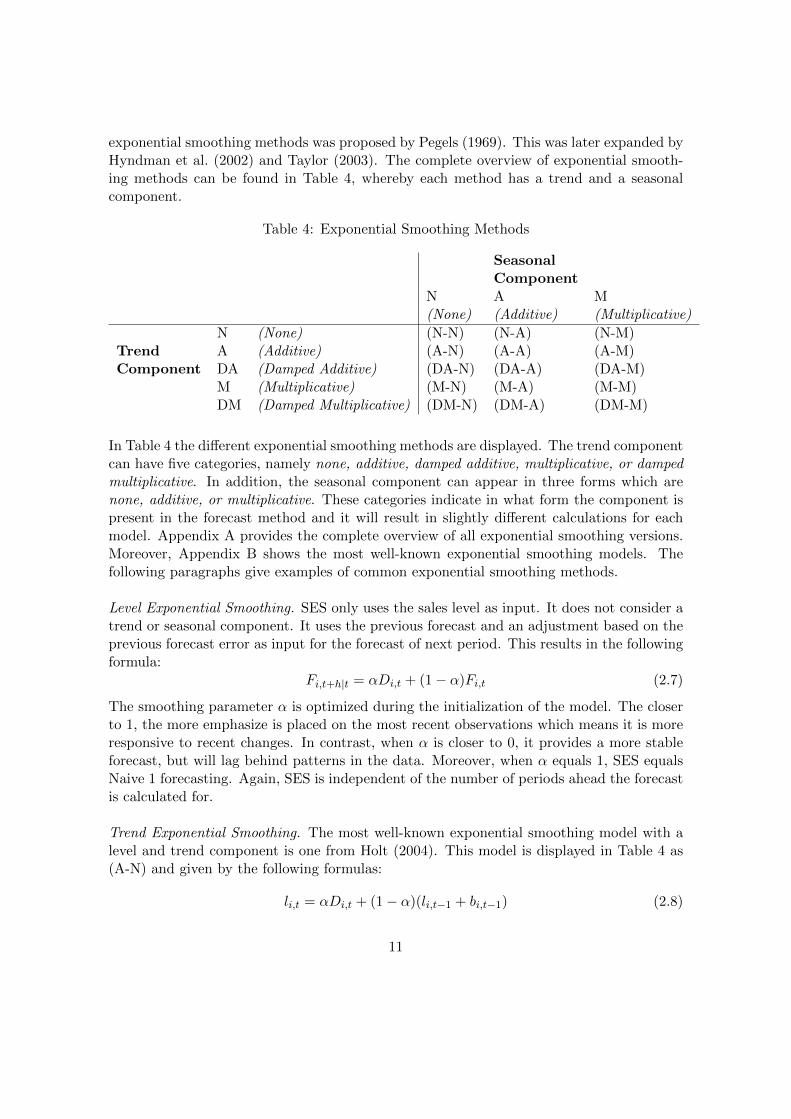
exponential smoothing methods was proposed by Pegels (1969). This was later expanded byHyndman et al. (2002) and Taylor (2003). The complete overview of exponential smooth-ing methods can be found in Table 4, whereby each method has a trend and a seasonalcomponent.

Table 4: Exponential Smoothing Methods

SeasonalComponent

N A M(None) (Additive) (Multiplicative)

N (None) (N-N) (N-A) (N-M)Trend A (Additive) (A-N) (A-A) (A-M)Component DA (Damped Additive) (DA-N) (DA-A) (DA-M)

M (Multiplicative) (M-N) (M-A) (M-M)DM (Damped Multiplicative) (DM-N) (DM-A) (DM-M)

In Table 4 the different exponential smoothing methods are displayed. The trend componentcan have five categories, namely none, additive, damped additive, multiplicative, or dampedmultiplicative. In addition, the seasonal component can appear in three forms which arenone, additive, or multiplicative. These categories indicate in what form the component ispresent in the forecast method and it will result in slightly different calculations for eachmodel. Appendix A provides the complete overview of all exponential smoothing versions.Moreover, Appendix B shows the most well-known exponential smoothing models. Thefollowing paragraphs give examples of common exponential smoothing methods.

Level Exponential Smoothing. SES only uses the sales level as input. It does not consider atrend or seasonal component. It uses the previous forecast and an adjustment based on theprevious forecast error as input for the forecast of next period. This results in the followingformula:

Fi,t+h|t = αDi,t + (1− α)Fi,t (2.7)

The smoothing parameter α is optimized during the initialization of the model. The closerto 1, the more emphasize is placed on the most recent observations which means it is moreresponsive to recent changes. In contrast, when α is closer to 0, it provides a more stableforecast, but will lag behind patterns in the data. Moreover, when α equals 1, SES equalsNaive 1 forecasting. Again, SES is independent of the number of periods ahead the forecastis calculated for.

Trend Exponential Smoothing. The most well-known exponential smoothing model with alevel and trend component is one from Holt (2004). This model is displayed in Table 4 as(A-N) and given by the following formulas:

li,t = αDi,t + (1− α)(li,t−1 + bi,t−1) (2.8)

11

bi,t = β(li,t − li,t−1) + (1− β)bi,t−1 (2.9)

Fi,t+h|t = li,t + hbi,t (2.10)

Gardner & McKenzie (1985) found that Holt’s method over-forecasted time series, especiallyfor larger forecast horizons. Therefore, they developed a dampening factor (φ). When φequals 1, the damped method equals Holt’s method. A damping method is used to dampthe trend factor in the model, which is expected to decline and stabilize on the long run.However, it is often not used to reduce model complexity.

Seasonal Exponential Smoothing. The seasonal component was first introduced in exponen-tial smoothing by Winters (1960). Holt and Winters together developed the Holt-Wintersexponential smoothing that considers both trend and seasonality in the time series. For thismethod both additive and multiplicative seasonality could be used. However, in practicemultiplicative seasonality is more common (Chopra & Meindl, 2016) which is displayed inTable 4 by (A-M). This method is calculated as follows:

li,t = αDi,t

Si,t−m+ (1− α)(li,t−1 + bi,t−1) (2.11)

bi,t = β(li,t − li,t−1) + (1− β)bi,t−1 (2.12)

Si,t = γDi,t

li,t−1 − bi,t−1+ (1− γ)Si,t−m (2.13)

Fi,t+h|t = (li,t + hbi,t)Si,t−m+h+m(2.14)

Intermittent & Lumpy demand. In this paragraph forecast methods dedicated to han-dle intermittent and lumpy demand are explained. In Section 2.1.1 intermittent demandis defined as an item with low demand size variation, but high inter-demand interval. Inaddition, lumpy demand has a high demand size variability and high inter-demand arrival,which make them more difficult to forecast (Syntetos et al., 2005).

Croston’s Method. Croston (1972) defined a forecast method to deal with demand intermit-tence or lumpiness based on the knowledge of exponential smoothing by Brown & Little(1956). However, Croston not only smoothed the demand size, but also the demand inter-arrival times. This is denoted in the following formulas:

If Di,t > 0, then:zi,t = δDi,t−1 + (1− δ)zi,t−1 (2.15)

pi,t = ηqi,t + (1− η)pi,t−1 (2.16)

If Di,t = 0, then:zi,t = zi,t−1 (2.17)

pi,t = pi,t−1 (2.18)

12

Where zi,t and pi,t represent the smoothed demand size and smoothed inter-arrival time ofproduct i at period t. In addition, qi,t is the number of periods since the previous demandobservation of product i at period t. δ and η represent the smoothing parameters for thedemand size and inter-arrival time. For both scenarios the forecast is calculated using:

Fi,t+h|t =zi,tpi,t

(2.19)

Croston’s method seemed promising, however, it has several pitfalls pointed out and im-proved by Syntetos & Boylan (2001) and Teunter et al. (2011). Syntetos & Boylan discoveredthat Croston’s method has a positive bias. In addition, it is not able to deal with obso-lescence issues, because it only updates the forecast after each period of positive demand(Teunter et al., 2011). Thus, it is possible that products that are not sold anymore stillhave a positive forecast due to Croston’s model definition. Syntetos & Boylan (2001) in-troduced the so-called Syntetos & Boylan Approximation (SBA) to avoid the positive biasof Croston. However, Syntetos et al. (2005) found that SBA did not perform best whencomparing it with SMAs, SES, and Croston forecasting. Leven & Segerstedt (2004) alsointroduced another Croston modification, however, again the disadvantage of this modelwas that it only updates after a positive demand observation.

Teunter et al. (TSB) Croston modification. Teunter et al. (2011) also proposed a modi-fication on Croston’s method, referred to as TSB. A disadvantage of Croston and Leven& Segerstedt is that they only update the forecast after a period of positive demand. Incontrast, TSB estimates the probability of non-zero demand (rather than interval size) andthe demand size. In that also updates its parameters every period which makes it morereactive to changes in the demand pattern. In addition, TSB makes use of two smoothingconstants, namely δ for the demand size and λ for the demand probability, because in gen-eral the demand probability is updated more often than the demand size. Also, note whenthe smoothing constants equal 1, TSB will result in Naive forecasting. Additionally, Teunteret al. (2011) has shown that TSB is less biased with stationary demand, linearly decreas-ing (increasing risk of obsolescence), and step-changed demand (sudden obsolescence) thanCroston’s method and SBA. However, the result is very sensitive to the chosen smoothingparameters. TSB is calculated as follows:

If Di,t > 0, then ci,t=1:

zi,t = zi,t−1 + δ(Di,t − zi,t−1) (2.20)

ci,t = ci,t−1 + λ(ci,t − ci,t−1) (2.21)

If Di,t = 0, then ci,t=0:zi,t = zi,t−1 (2.22)

ci,t = ci,t−1 + λ(ci,t − ci,t−1) (2.23)

Where ci,t represent the demand indicator for product i at period t which equals 1 if apositive demand has occurred for product i at period t, and 0 otherwise. In addition,

13

ci,t estimates the probability of demand of product i at period t. For both situations theforecast is calculated by:

Fi,t+h|t = zi,tci,t (2.24)

2.1.3 Demand Forecast Evaluation

Forecast models will always result in errors (Silver et al., 1998), therefore, to improve theforecast decision making errors should be tracked. However, Armstrong & Collopy (1992)stated that one single metric cannot provide an unambiguous conclusion of the forecastmodel performance. Over the years different metrics have been proposed which are classifiedin four groups by Hyndman & Koehler (2006). In the following paragraphs these groupsare discussed. Additionally, several other metrics are presented. Forecast error for producti at period t is defined as follows:

Ei,t = Di,t − Fi,t (2.25)

Scale-dependent measures. As the name suggest, scale-dependent measures dependon the scale of the data. These metrics are best used when comparing different forecastmethods on the same data set. Their applicability when comparing different data sets islimited due to data scale influence on the performance indicators. The most commonly usedscale-dependent measures are MAE, Mean Squared Error (MSE), and Root Mean SquaredError (RMSE). Historically, RMSE and MSE have been popular due to their theoreticalrelevance in statistical modeling (Hyndman & Koehler, 2006). However, these metrics aremore sensitive to outliers, which lead to criticism from several authors and their advice tonot use these metrics as forecast accuracy measures (Armstrong (2001); Chatfield (1988)).In addition, MAE is easy to understand and calculate, while RMSE is more difficult tointerpret (Hyndman & Athanasopoulos, 2018).

Mean Absolute Error (MAE) =1

T

T∑t=1

|Ei,t| (2.26)

Mean Squared Error (MSE) =1

T

T∑t=1

E2i,t (2.27)

Root Mean Squared Error (RMSE) =

√√√√ 1

T

T∑t=1

E2i,t (2.28)

Syntetos et al. (2005) recommended another scale-dependent measure for intermittent de-mand specifically, namely Geometric MAE (GMAE), however due to intermittent demandcharacteristics GMAE might be inappropriate to use as forecast accuracy measure (Boylan& Syntetos, 2006).

14

Percentage error measures. Percentage errors have the advantage of being scale-independent,thus are frequently used to compare forecast performance across different data sets. How-ever, they are infinite or undefined when the sales value is (close to) zero. Several well-knownpercentage error measures are Mean Absolute Percentage Error (MAPE) and Root MeanSquared Percentage Error (RMSPE). MAPE was also the primary metric in the first M-competition of Makridakis et al. (1982). A drawback of MAPE is its asymmetry since aforecast error larger than the actual demand observation results in a larger MAPE com-pared to an equal forecast error below the actual demand observation (Makridakis et al.,1993). Therefore, a symmetric MAPE (sMAPE) has been developed and tested in the thirdM-competition (Makridakis & Hibon, 2000).

Mean Absolute Percentage Error (MAPE) =1

T

T∑t=1

|100Ei,tDi,t

| (2.29)

Symmetric Mean Absolute Percentage Error (sMAPE) =1

T

T∑t=1

200 ∗ |Di,t − Fi,t|Di,t + Fi,t

(2.30)

Root Mean Squared Percentage Error (RMSPE) =

√√√√ 1

T

T∑t=1

(100Ei,tDi,t

)2 (2.31)

Median measures were introduced to avoid extreme values (Armstrong & Collopy, 1992).Still, all percentage error measures only make sense for forecasting data with a meaningfulzero (Hyndman & Koehler, 2006). For example, they are not suitable for measuring theforecast error of temperatures on Celsius or Fahrenheit scales. There is still some discus-sion on whether symmetric measures are actually symmetric (Goodwin & Lawton (1999);Koehler (2001)). Also, Kolassa & Martin (2011) stated that percentage forecast errors arebiased in general.

Relative error measures. The next group of forecast error measures are relative errormeasures, which are also scale-independent. They use an alternative way of scaling, becauseit divides each calculated error by an error obtained using a benchmark forecast method(E∗i,t). A commonly used benchmark method is naive forecasting. An advantage of relativeforecast measures is the ease of understanding. If the relative error is greater than 1, themain forecast method performs worse than the benchmark. In contrast, a value lower than 1indicates the opposite. The most popular relative error measure is Mean Relative AbsoluteError (MRAE).

Ri,t =Ei,tE∗i,t

(2.32)

Mean Relative Absolute Error (MRAE) =1

T

T∑t=1

|Ri,t| (2.33)

15

However, Hyndman (2006) indicated that when errors are small, which can occur often withan intermittent demand pattern, the use of benchmark methods such as naive forecastingcan lead to division by zero. For that, Armstrong & Collopy (1992) recommended to trimthe extreme values by using ’winsorizing’, which avoids the difficulties with small values, butincrease the calculation complexity. In addition, the statistical distribution of relative errorswill result in an undefined mean and infinite variance (Hyndman & Koehler, 2006).

Scale-free measures. Relative error measures try to remove the scale of the data bycomparing the data with some benchmark method. However, this is only possible whenboth forecasts are calculated on the same demand data. Therefore, Hyndman & Koehler(2006) developed a scaled error based on the in-sample MAE from the naive forecastingmethod, which overcomes the previously described issues. A scaled error is below one if itarises from a better forecast than the average one-step ahead naive forecast computed in-sample. In contrast, it is greater than one if the forecast is worse than the average one-stepahead naive forecast. A drawback is this scale-free measures is being infinite or undefinedwhen historical demand observations are equal.

Other measure. Bias indicates if the forecast method reflects the underlying demandpattern by checking if the forecast errors are randomly distributed around 0 (Chopra &Meindl, 2016). Additionally, a large positive or negative bias value can indicate a biasedforecast, which calculate by Equation 2.34. Another measure to indicate possible forecastbias is the tracking signal (Blackstone, 2010).

Biasi,T =

T∑t=1

Ei,t (2.34)

2.1.4 Contribution to the literature

As mentioned by Stevenson (2011), forecasts are used to make important decisions in acompany’s supply chain management process. In addition, it has a large impact on thecustomer’s order fulfillment requirements Reiner & Fichtinger (2009), which was also em-phasized by Armstrong (1988). Moreover, over the years a tremendous amount of researchhas performed on forecasting techniques and evaluations. Therefore, this work will pro-vide an empirical study on different demand classification schemes using 46 SKUs of a fastmoving consumer good (FMCG) environment. In addition, it will provide a case studythat investigates the effects of different forecasting models on the forecast accuracy in thischallenging environment. Moreover, it gives an analysis on the forecast accuracy of thequalitative forecasting methods currently used. Finally, it will investigate the effect of aredesigned forecast model on the inventory control system.

16

2.2 Research Questions

In this section the research questions and the sub research questions are discussed. Thisresearch aims to discover opportunities for BNE to improve the forecast accuracy of theNordic market. To reach this goal the following main research question and sub researchquestions are defined.

Main Research Question:How can a redesigned forecast model be used to improve the Nordic forecast accuracy whileincreasing the stock performance and product availability to customers?

2.2.1 Sub Research Questions

In order to answer this main research question, several sub research questions (SRQs) aredefined. These are defined as follows:

SRQ 1: What are the relevant characteristics of the assortment in scope?

SRQ 2: Which forecast methods that have been applied in a similar environment are de-scribed in the literature?

SRQ 3: What forecast model can be designed that accounts for the different characteristicsof the assortment in scope?

SRQ 4: How does the current forecasting method for promotional sales perform?

SRQ 5: How does the redesigned forecast model perform compared to the current forecastmodel?

SRQ 6: What is the impact of the redesigned forecast model on the stock performanceand product availability to customers?

2.2.2 Deliverables

This work should contribute to both the needs of the company as well as the academics.Therefore, a list of deliverables has been formulated. For each deliverable is indicated whichSRQ fulfills this deliverable (DEL).

DEL 1: Describe the characteristics relevant to forecast the assortment in scope (SRQ 1)

DEL 2: Provide different forecast methods described within the literature that have beenused in a similar environment (SRQ 2)

DEL 3: Design a forecast model for the assortment in scope (SRQ 3)

17

DEL 4: Evaluate the current used forecasting method for promotional sales (SRQ 4)

DEL 5: Simulate the redesigned forecast model, compare it to the current forecast model,and analyze the differences (SRQ 5)

DEL 6: Suggestions for the implementation of the new redesigned forecast model, if itoutperforms the current model, in the FM environment (SRQ 5)

DEL 7: Investigate the impact of the new forecast model on forecast accuracy whileincreasing the stock performance and product availability to customers (SRQ 6)

2.3 Scope

An overview of the scope of this work is given in this section. As mentioned before, thiswork focuses on the Nordic region of BNE, which means that the Benelux is out of scopeof this work. This Nordic region consists of Denmark, Norway, Sweden, and Finland. Inthe Nordic region two types of customers are served, retail customers such as supermarketsand food service customers such as restaurants. These customer sections are both includedin the scope of this work. In addition, both canned and frozen products sold are included.

Besides, the baseline sales is chosen as the main focus, which means that the redesignedforecast model will be applicable for the baseline sales only. This makes sense, because thepromotion forecast is calculated in a different tool. In addition, based on data availabilitythe selection of specific products in scope has been determined, which is further explainedin Section 4.1.1.

18

3 Case study current supply chain operations

In this chapter, the current supply chain operations of the case study company are studiedin more depth. First of all, Section 3.1 the current demand forecasting techniques aredescribed. Next, in Section 3.2 the current inventory control policy is explained.

3.1 Demand forecast

This project focuses on the forecasting of future demand in the Nordic countries BNEis operating. In the following sections the different demand forecast techniques that arecurrently used are described in detail.

3.1.1 Main forecast model

Each product’s forecast consists of two parts, namely baseline and promotion forecast. Ev-ery part is determined using its own forecast method and the results are summed afterwardsto derive the total forecast for a specific period. For each product sales observation data isaggregated weekly due to frequent zero demand observations on a daily basis, promotionsschedules that are planned on weekly basis, and to be consistent with the review periodwhich is once a week. This weekly sales data is only saved for the current book year dueprogramming limitations. Therefore, as explained later in this work, historical monthlydata is manually split into weekly data.

Baseline forecast The baseline forecast is determined using FM’s historical baseline salesdata. The demand planner chooses an available model to calculate the forecast. This choiceis based on the calculated MAE, exogenous knowledge about future periods, or demandplanner experience. When the model is chosen, FM calculates the best fitting parametersfor this model based on the historical sales data and uses these model parameters to forecastfuture demand. FM is also able to indicate the best fitting model itself based on the MAEcalculated over a pre-determined historical interval. The historical interval length for thisbest fitting model is determined by the demand planner which indicates the relative impor-tance of fitting recent or older data observations correctly. At this point BNE often usesa level shift model, also known as moving average, to forecast demand. Other models orthe best fit model are rarely considered yet. Moreover, as mentioned before FM is also ableto integrate trend and seasonality characteristics in the chosen forecast model. However,at this point this is also hardly considered yet. Therefore, this gives the opportunity toinvestigate an improved method to forecast future baseline demand.

An important note here is that FM interprets level, trend, and seasonality different thanacademic literature. First of all, level and trend are combined in the FM parameter trend,which is uncommon in academic literature. Second, FM usually includes a seasonalityfactor, which can appear in different forms. This means that to determine the final forecastin FM the so called trend of the model is multiplied with a weekly seasonality based onhistorical sales, even if historical seasonality does not make sense.

19

Promo forecast. In contrast, the promotional forecast is not calculated using a forecasttool like FM. This forecast is determined by the sales team. They base their forecast oninformation retrieved from close contact with the customer and possible contracts signed.In addition, there is no model behind this calculation that takes into account for examplecannibalization with other products or the influence on the sales of other Bonduelle cus-tomers. Moreover, it works separately from the baseline sales forecast model, which meansthat the baseline sales is not adjusted in promotion weeks. At this point, there is no checkif the promotional forecast determined by the sales team is reflecting the actual sales to thecustomers. Therefore, this gives the opportunity to investigate the current performance ofthis promotional demand forecast.

3.1.2 Manual Adjustments

The forecasting methods as described in Section 3.1.1 do not lead to satisfying FA results.Therefore, in some situations manual adjustments are performed. Examples are when amajor customer decides to not order anymore, while the forecast is still based on also thesales to this customer. There are several ways a manual adjustment can be performed,namely by a percentage or factor, or an change in the model assumptions.

These manual adjustments often result from so called Supply & Operations Planning(S&OP) meetings. This meeting is held every month with several departments to review theforecast and to compare the actual sales with the budget. The main departments involvedare supply chain and sales. The supply chain department has access to the quantitativedata resulting from FM, while the sales department has more information about qualita-tive data such as expected trends, new customers, and promotions. This information couldlead to adjustments in the forecast given by FM. For example, when the sales team hasestablished a contract with a new customer the forecast should be increased. Thus, manualadjustments are performed based on exogenous information to FM up- or downgrade theforecast with a factor or percentage or by adjusting the existing model assumptions. Anexample of this could be changing the start date the model is calculated on.

3.1.3 Forecast Performance Indicators

Even after possible manual adjustments, the final Nordic forecast does not lead to a sat-isfactory FA (as mentioned in Section 1.2). Therefore, methods to improve the Nordic FAare high on the agenda of BNE. In addition, as already mentioned in Section 1.2, the FA isthe most important performance indicator of forecast, its calculation is given in Equation1.1.

3.2 Inventory control

Forecasting has a large impact on inventory control, therefore, this paragraph is dedicatedto indicate the importance of correct forecasting for the inventory control.

20

Inventory Control Model. Currently no automatic Enterprise Resource Planning (ERP)system is controlling the inventory. This is manually done by the supply chain coordinatorfollowing the procedure as explained in this section. For each product, the stock level ischecked every week to determine if new products must be ordered. This means the stock isreviewed every week, which results in a review period of 1 week. The height of the replen-ishment order is calculated based on the reorder level. This reorder level is the based on twocomponents, the expected demand during review period plus lead time and safety stock. Ifat the review moment the inventory position, which is inventory on hand (inventory phys-ically available) and pipeline inventory, is below the reorder level a new order is placed.The height of the replenishment order is n times the case pack size such that the inventoryposition is raised at or above the reorder level. The safety stock is determined using anABC classification model, which categorizes each product in one of the three groups basedon the average number of boxes sold per week of the last 52 weeks. The categories are asfollows; products in category A have an average weekly sales of more than 50 boxes perweek, which assigns them a safety stock of 3 weeks average sales. B products have a salesbetween 25 and 50 boxes per week, which results in a safety stock of 4 weeks average sales.Lastly, products in category C have an average sales below 25 boxes per week and will havea safety stock of 5 weeks average sales. This is displayed in Figure 5.

Table 5: ABC safety stock classification

CategoryAverage sales volume(in boxes per week)

Safety stock(in weeks average demand)

A >50 3B 25-50 4C <25 5

The current inventory policy used by the Nordic warehouse in Denmark is in the literatureknown as the (R,s,nQ) policy. In which R represents the review period, s the reorder level,n the order quantity, and Q the case pack size. This policy is displayed in the followingfigure 6. As displayed in red, BNE allows back orders using this policy. In addition, τ isan arbitrary point in time at which inventory position is reviewed. Then an order is placedwhich raises the inventory position above the reorder level of 22 and this order is receivedL periods later at τ + L. At τ + R the inventory position is again review, so R indicatesthe review period.

21

Figure 6: (R,s,nQ) inventory control policy (van Donselaar & Broekmeulen, 2017)

The standard (R,s,nQ) policy is adjusted by BNE, because replenishment orders are donein Full Truck Loads (FTLs). Each truck has 33 pallets places, which means that the totalreplenishment order must equal a multiple of 33. When this does not hold, the replenish-ment order is manually adjusted to fulfill the FTL requirement. For example, in the mostextreme case where the initial replenishment order equals 34 pallets, the total number ofpallets ordered is manually increased to 66 to completely fill the 2 trucks. The determi-nation of which 32 pallets are added to the order is done by the supply chain coordinatorbased on simple calculations and experience. This means that the truck is filled with palletsof different products. Thus, the inventory control policy that is used by Bonduelle is betterdescribed as a policy which base is established by the standard (R,s,nQ) inventory controlpolicy, but changed when implementing the full truck load heuristics.

A notable aspect is that this replenishment system does not take into account the perisha-bility of products. Therefore, it is of great importance forecasts are accurate. First of all,to guarantee product availability for customers. Second, to avoid overstock when unsoldpossibly result in violated BBD restrictions.

3.2.1 Inventory Control Performance Indicators

In order to determine the inventory control performance, several indicators have been es-tablished. First of all, to calculate the product availability to customer the fill rate is used.This service level is the number of boxes that could be directly delivered from inventoryon hand divided by the total amount of boxes that must be delivered to customers. Thetotal amount of boxes to be delivered are demand in the period plus the back orders fromprevious period.

22

FRi,t =#Boxes product i delivered in period t

# Demand product i in period t + #Back orders product i in period t-1(3.1)

This is the service level for one single product i at period t. In order to achieve theaggregated fill rate for all products in a specific period t a weighted fill rate is used andcalculated as follows:

FRt =

I∑i=1

wi,t ∗ FRi,t (3.2)

Where:

wi,t = weight of product i at period t withI∑i=1

wi,t = 1

=Di,t∑Ii=1Di,t

(3.3)

This aggregated fill rate consists of the individual fill rate using Equation 3.1 for eachproduct i multiplied with the weight of this product. This weight is determined using thedemand per period for product i divided by the total demand of all products together.

Second, to determine the stock performance several stock related indicators are calculated.The first indicator is the physical inventory to track the average amount of products on stockwhich are used to calculate the inventory holding costs. Second, is the number of back ordersis tracked to indicate the possibility to deliver directly from stock. For example, short-termback orders are allowed by the customers, however, in the case of long-term back orderscustomers might search for other suppliers which is harmful for BNEs business.

23

4 Data analysis

In this chapter the available sales data is discussed. First, the rules to include a productin the scope are discussed. Then, the data split from monthly to weekly basis is explained.Also, the existing demand pattern characteristics are elaborated.

For this thesis, time series forecasting methods are used, which assume that historicalsales data is a good indicator to predict future demand. This is why the historical salesdata is used in this work. This chapter explains the data cleaning methods as well as thedemand characteristics. This ensures a clean and workable data set. In addition, basedon the demand characteristics found in the baseline sales, different forecast methods couldbe applied as explained in Chapter 5. For example, trend or seasonality characteristicsstimulate the use of forecast methods including those characteristics like Holt or Holt-Winters.

4.1 Baseline Data Analysis

4.1.1 Products in scope

The baseline products in the scope of this project are determined based on three subjects,which are geographical location, product categories, and product maturity.

Geographical Location. First, this thesis uses data of all the products sold in the Nordiccountries. This includes both canned and frozen products, which are sold in the retail orfood service segment. In addition, these products can be delivered directly from the factoryto the customers or first stored in the Nordic warehouse in Denmark. This depends on thetype of product, order size, or delivery agreements with the customers.

Product Categories. All product groups of BNE are in scope of the project. For theNordics this means both canned and frozen products. In addition, both products from theretail and food service businesses.

Table 6: Total Nordic products in categories

Canned Frozen Total

Retail 107 0 107Food Service 44 33 77

Total 151 33 184

The total number of products sold in the Nordics is 184. This set of products includes 151canned products, which is about 82.1%, and 33 frozen products that account for 17.9%. Inaddition, the products can be split based on business. This resulted in 107 retail productsand 77 food service products, respectively 58.2% and 41.8% of the products sold in theNordics.

24

Product Maturity. Furthermore, to determine a forecast model historical sales data isneeded. It is used to initialize parameters and to simulate the performance of different fore-cast models. Therefore, this work only considers matured products, which does not includephasing in or phasing out products. The phasing in products are excluded, because too fewdata points are available. Moreover, these data points are highly sensitive to the mannerand timing of the product introduction. The phasing out products are also excluded fromthe scope, because they often have an extremely downward trend and once sold out theproducts is removed from the assortment. Thus, they are of less interest for the company.The following rules are used to define a matured product:

1. Monthly sales data available from July 2017 till December 2019To ensure there is enough historical data available.

2. At least 7 months of sales in 2019To overcome that (more than) half of the months in 2019 have zero demand occurred.In addition, it ensures that the product is still active.

3. Maximum 12 months of zero salesTo ensure there is enough data available to initiate the model parameters and to checkthe model performance.

BNE’s goal is to use the 80/20 rule, which means that the products included in the scopeshould cover about 80% of the total sales. After applying these maturity rules, the productsconsidered lead to 75% of the sales in 2019, which made these products valid. The finalproducts that are used are the following:

Table 7: In scope Nordic products in categories

Canned Frozen Total

Retail 24 0 24Food Service 19 3 22

Total 43 3 46

As can be seen in Table 7, 46 products are considered in scope of this work of which themajority are canned products, namely 93.5%. This is reasonable, because frozen productsare only introduced in the FS section. In addition, phasing in and out of products in thedata set had a large influence on the number of products excluded from the scope.

In order to indicate the need for a better forecast method, the FA of the products in scopeis shown in Figure 7. As can be seen, the retail products have a low FA of 22.7% in 2019.Therefore, the need for a better forecasting method for the retail business is proven. Incontrast, the FS business shows nearly satisfying FAs each month except for December2019 on average 63.5%. In December 2019 an enormous out of stock has taken place on themajor products sold in the FS business. Based on only this figure there could be concluded

25

that the FS business displays no need for a redesigned forecast model. However, the firstquarter of 2020 resulted in a FA of 49.2% for the same set of products, therefore it isstill necessary to improve the forecast methods used for the FS business even if the overallimprovement potential might be lower than for the retail business.

Figure 7: Forecast Accuracy Nordics 2019 in scope products

4.1.2 Data Conversion

Currently, only monthly sales data with a split in baseline and promotion sales is available.To investigate any effect on stock performance and product availability for the baselinesales, the monthly sales must be converted into weekly sales to fit into the (R,s,nQ) inven-tory control policy as will be further explained in Section 5.2. In this work three methodsto split monthly sales data will be used, which are explained below:

1. Average weekly salesThe monthly sales are equally spread over the weeks.

2. Intermittent weekly salesThe monthly sales for uneven months are all ordered in the first week of the month,while the monthly sales for even months are all ordered in the last week of the month.

3. Random weekly salesThe monthly sales are ordered during random weeks of the month. In addition, thedemand size is randomly spread over those weeks.

These splitting methods are used to indicate different levels of demand intermittence anddemand size variability. In Chapter 6 the average results of these three types of weeklysales will be displayed unless mentioned otherwise. There is assumed that a combinationof three months follow a ’4-4-5’ weekly pattern, which means that for each quarter the first

26

and second month have 4 weeks and the third month 5 weeks. This is done to still achieve52 weeks in a year. Thus, every March, June, September, and December has 5 weeks, whilethe other months consist of 4 weeks. The first method, average, is considered to displaythe sales data as if in each week of a specific month the same volume is ordered. Thismethod is considered as the least challenging in terms of intermittence and demand sizevariability. The second method, intermittent, is considered to display a weekly pattern thatincludes the maximum level of demand inter-arrival time and demand size variability. Thelast option, random, is used create medium intermittence and sales size variability. For thismethod the monthly sales is ordered in a random amount of weeks of the month, then thereis randomly chosen which weeks will have sales, and the sales amount is again randomlyspread over the weeks with sales. This is organized in the following procedure:

1. Number of weeks with sales (n)Consider a month that has X weeks. A random generator will give a value between1 and X to indicate the number of weeks of that month will contain sales value.The month January is taken for this example. The month January has 4 weeks andbased on this procedure n equals 3 for this month.

2. Specify sales weeksBased on step 1, the value n is randomly chosen. In this step n unique numbers aregenerated between 1 and X to indicate which weeks of the month will have sales.Based on the first step, 3 weeks of January will contain sales. The second step providesthe values 1, 3, and 4, which means that the sales of January will occur in week 1, 3and 4 of January.

3. Specify sales valueIn this step n values are randomly draw from a uniform distribution between 1 and1,000, namely U1, ..., Un. The fraction of monthly sales in each of the n weeks equalsits uniform distribution value divided by the sum of all n uniform distribution values,

Ui∑ny=1 Uy

.

The 3 uniform distribution values are 798, 83, and 619, and the monthly sales ofJanuary was 10,000kg. Then the first week will contain 798

1,500 ∗ 10, 000 = 5, 320kg, thethird week 553kg, and the fourth week 4,127kg. Note here that the second week willhave zero sales, because step 2 determined that no sales will be dedicated to this week.

4.1.3 Demand Patterns

Syntetos & Boylan Demand Classification. In Section 2.1 the Syntetos & Boylandemand classification scheme has been presented. It fits demand patterns in four categoriesbased on demand size variation and demand inter-arrival time. The four categories areerratic, lumpy, smooth, and intermittent. This classification scheme is first used withmonthly data of the products in scope based on the rules defined in Section 4.1.1. Thisresults in Figure 8, which shows that based on monthly basis out of the 46 products in scope26% is classified erratic, 15% lumpy, and 59% smooth. In addition, none of the products inscope is characterized as intermittent. There can be concluded from this that on a monthly

27

basis most products display a smooth demand pattern. However, the weekly sales patternsplit defined in 4.1.2 might imply different demand patterns on a weekly basis.

Figure 8: Syntetos & Boylan classification on monthly data

In Figure 9 the Syntetos & Boylan classification based on weekly data is displayed. Theleft diagram shows the classification on weekly average data, which is quite similar to themonthly data. Only one product switched from smooth to erratic. However, as can be seenin central and right diagram, when considering the weekly intermittent and weekly randomdata only lumpy demand patterns are discovered. These classification diagrams indicatethe importance of a forecast model that includes demand intermittence, because the currentforecast model does not deal well with this yet.

Figure 9: Syntetos & Boylan classification on weekly data

Trend and Seasonality. Stationary demand is defined as ’a time series whose propertiesdo not depend on the time at which the series is observed’ (Kwiatkowski et al., 1992). Trendand seasonal behavior are characteristics of non-stationary demand. In order to indicatethat trend and seasonality are important factors to consider when redesigning the forecastmodel Figure 10 is displayed.

28

Figure 10: Total Monthly Sales

Figure 10 displays three concepts; actual monthly sales observations, linear regression basedon actual sales observations, and linear regression based on actual sales observations with aseasonal factor. The actual sales are represented in the bars, which show a similar patternevery 6 months. Second, a significant linear regression is calculated using the real salesdata of each month shown in the blue bars. As can be seen a positive trend is found,because the orange line has positive slope. Lastly, the linear regression is adjusted withan average monthly seasonal factor by multiplying linear regression value by the averagemonthly seasonal factor. Each monthly seasonal factor is calculated by dividing the realsales by the linear regression value. For each month these seasonal factors are averaged toderive the average monthly seasonal factor. This seasonal factor is then multiplied with theresult from the linear regression to calculate the value of a linear regression with a seasonalfactor. From this can be concluded that trend and seasonal factors should be consideredwhen redesigning the forecast model.

4.2 Promotion Data Analysis

In order to analyze the current promotion practices the so-called campaign schedule isused. This format was introduced at BNE in the beginning of 2019, because the forecasttool does not show promotion forecasts that are planned in the long-term future (severalmonths ahead). Therefore, this schedule was introduced to track campaign or promotionplanning of the Nordic customers on the long run. This schedule includes among otherthings customer and product information, quantity information, and planning information.

To achieve a workable data set the following rules and assumptions are used. First ofall, only promotions held between January 2019 and April 2020 are included in the scope.Because in the promotion forecast tool the forecast quantities and weeks are turned into

29

actual quantities once the order is received. Moreover, when the date of the forecast haspassed, the promotion forecast disappears in the system. Therefore, only campaigns thatare included in the campaign schedule are used. Second, promotions missing essential dataare excluded from the scope. By essential data is meant the following information; forecastquantity, forecast date, promotion in store date, actual quantity, actual sales date, productnumber, and customer. Finally, when the promotion is cancelled it is excluded from thescope. This resulted in a total set of 205 promotions. These promotions are held for 44different products and 14 different Nordic customers.

30

5 Forecast and inventory control policies

In this chapter the thesis policies are discussed. First, the chosen forecast models arediscussed in Section 5.1. Second, in Section 5.2 the inventory control policy used in thiswork is explained.

5.1 Forecast Policy

The main concern of BNE is an unsatisfying FA. The current forecasting practices giveopportunities to investigate using different forecast methods. This section explains theforecast policy for the baseline sales and its key performance indicators (KPIs). In addition,it defines the promotion forecast KPIs.

5.1.1 Baseline Policy

In this section the baseline forecast policy will in this work be discussed. Moreover, itsrelevant KPIs will be defined.

Baseline Forecast Policy. In Section 4.1.3 there has been shown based on the classifi-cation of Syntetos et al. (2005) different demand patterns are identified for the products inscope, namely smooth, lumpy, and erratic. These demand patterns indicate that demandinter-arrival time variability (intermittence) and demand size variability play a role in thefaced sales. Therefore, forecast models that include those characteristics are considered asredesigned forecast models. The following models implemented in this work are divided inthree categories, namely: smooth models, intermittent & lumpy models, and newly designedmodels. The smooth models are the following; SES, Holt’s additive trend, and Holt-Winters’additive trend with multiplicative seasonality. The intermittent & lumpy models are Cros-ton and TSB. Finally, the newly designed forecast models are Croston with additive trend,Croston with additive trend and multiplicative seasonality, TSB with additive trend, andTSB with additive trend and multiplicative seasonality. These newly designed models couldalso be classified as Croston and TSB combined with Holt’s and Holt & Winters’s models.These models are chosen for several reasons. First of all, the models include trend andseasonality factors, which were also found is Section 4.1.3. Second, Croston and TSB takeboth the demand inter-arrival time variability and demand size variability into account. Inthe following paragraphs the initialization, forecast model components, and parameters areelaborated. To clarify, only the weekly sales data of 2017 and 2018 is used to train themodels and optimize its parameters, the weekly sales of 2019 is used to test the models.

SES. SES forecasting uses Equation 2.7 to determine the h-period ahead forecast. In orderto initialize the model Fi,0 is needed, which is assumed to be the average weekly sales of2017 and 2018.

Holt. Holt’s forecast model uses Equation 2.8 to determine the level component, Equation2.9 for the trend component, and Equation 2.10 to calculate the h-period ahead forecast.

31

The initial values for level and trend, respectively li,0 and ti,0, are calculated by a linearregression over the weekly sales of 2017 and 2018, where the intercept equals the initial leveland the slope the initial trend component.

Holt-Winters. Holt-Winters’ seasonal exponential smoothing forecast with additive trendand multiplicative seasonality consists of three components, namely level, trend, and season-ality. These are calculated using respectively Equation 2.11, 2.12, and 2.13. The h-periodahead forecast is determined by Equation 2.14. The initial values of level and trend areagain calculated by a linear regression over the weekly sales of 2017 and 2018. The initialseasonal factors of each week are determined by averaging the weekly seasonal factor of theyears 2017 and 2018. This factor equals

Di,t

li,0+bi,0∗t , so the actual demand of period t divided

by the value resulting from the regression at period t.

Croston. The Croston’s forecast model is based on a demand size and inter-arrival timeestimation. When the sales at period t equal zero, Equation 2.17 and 2.18 are used, whilewith sales larger than zero Equation 2.15 and 2.16 are used. The forecast in both casesis calculated using equation 2.19. The initial values for zi,0, pi,0, and qi,0 are estimatedas follows; the demand size for period 0 is equal to the average weekly sales of 2017 and2018. The demand inter-arrival time and number of periods since previous sales at period0, respectively pi,0, and qi,0, are assumed to be 1 and 0. This implies that the expectedinter-arrival time is 1 period and that positive sales have occurred in period 0.

TSB. TSB forecasts are calculated using Equation 2.22 and 2.23 for the demand size anddemand probability estimators when the sales of period t equal zero. When the sales aregreater than zero, Equation 2.20 and 2.21 are used. The forecast is calculated using Equa-tion 2.24. The initial demand size estimation of period 0 is set to the average weekly sales of2017 and 2018. In addition, the probability estimation of period 0 equals 1, which impliesthat a positive demand is expected with 100% probability.

Holt-Croston. The Holt-Croston forecast model is a combination of the Holt’s trend expo-nential smoothing with additive trend and Croston’s forecast model. The calculations arevery similar to the individual models, however, the complete overview of formulas is givenbelow. First of all, while the demand size estimator of Croston’s model was only based onSES, now a trend factor is included which is shown in Equation 5.2 and 5.6. This results ina demand size estimator depending on the forecast horizon h, which is shown in Equations5.3 and 5.7. The initial values for level and trend, li,0 and ti,0 are again calculated by alinear regression over the weekly sales of 2017 and 2018, where the level is the intercept andtrend is the slope of this regression. Similar to Croston’s model the pi,0 and qi,0 are set to1 and 0.

If Di,t > 0, then:li,t = αDi,t + (1− α)(li,t−1 + bi,t−1) (5.1)

bi,t = β(li,t − li,t−1) + (1− β)bi,t−1 (5.2)

32

zi,t+h|t = li,t + hbi,t (5.3)

pi,t = ηqi,t + (1− η)pi,t−1 (5.4)

If Di,t = 0, then:li,t = li,t−1 (5.5)

bi,t = bi,t−1 (5.6)

zi,t+h|t = li,t + hbi,t (5.7)

pi,t = pi,t−1 (5.8)

The forecast is calculated by the demand size estimation divided by the expected inter-arrival time at period t.

Fi,t+h|t =zi,t+h|t

pi,t(5.9)

Holt-Winters-Croston. The Holt-Winters-Croston forecast model is a combination of theHolt-Winters’s additive trend with multiplicative seasonality exponential smoothing andCroston’s forecast model. This model consists of four components, namely level, trend, sea-sonality, and inter-arrival time estimations. The estimation of level, trend, and seasonalityis combined in the component demand size (zi,t+h|t). The initial values for level and trendare again retrieved from a linear regression over the weekly sales of 2017 and 2018. Theseasonal factor is determined using the same approach as explained in the Holt-Winters’smodel. The initial values for demand inter-arrival time and number of periods since lastsales occurrence are again set to 1 and 0. The complete model is represented by Equation5.10 to 5.20.

If Di,t > 0, then:

li,t = αDi,t

Si,t−m+ (1− α)(li,t−1 + bi,t−1) (5.10)

bi,t = β(li,t − li,t−1) + (1− β)bi,t−1 (5.11)

Si,t = γDi,t

li,t−1 − bi,t−1+ (1− γ)Si,t−m (5.12)

zi,t+h|t = (li,t + hbi,t)Si,t−m+h+m(5.13)

pi,t = ηqi,t + (1− η)pi,t−1 (5.14)

If Di,t = 0, then:li,t = li,t−1 (5.15)

bi,t = bi,t−1 (5.16)

Si,t = Si,t−m (5.17)

zi,t+h|t = (li,t + hbi,t)Si,t−m+h+m(5.18)

33

pi,t = pi,t−1 (5.19)

The forecast is again calculated by the demand size estimation divided by the expectedinter-arrival time at period t.

Fi,t+h|t =zi,t+h|t

pi,t(5.20)

Holt-TSB. The Holt-TSB forecast model expands Holt’s trend exponential smoothing modelby introducing a demand probability factor as used by Teunter et al. (2011) in their TSBmodel. In this model the demand size is estimated using a level and trend component,which are given in Equations 5.21 and 5.22 and Equations 5.25 and 5.26. As mentionedbefore, level and trend are estimated using a linear regression over the weekly sales of 2017and 2018. By introducing a trend component in the model, the demand size estimator isdependent on h which is displayed in Equation 5.23 and 5.27. Again, the demand proba-bility estimation of period 0 is set to 1, which means that demand is expected with 100%probability.

If Di,t > 0, then ci,t=1:

li,t = αDi,t + (1− α)(li,t−1 + bi,t−1) (5.21)

bi,t = β(li,t − li,t−1) + (1− β)bi,t−1 (5.22)

zi,t+h|t = li,t + hbi,t (5.23)

ci,t = ci,t−1 + λ(ci,t − ci,t−1) (5.24)

If Di,t = 0, then ci,t=0:li,t = li,t−1 (5.25)

bi,t = bi,t−1 (5.26)

zi,t+h|t = li,t + hbi,t (5.27)

ci,t = ci,t−1 + λ(ci,t − ci,t−1) (5.28)

The forecast is determined by multiplying the demand size estimation with the demandprobability estimation. This is represented in Equation 5.29.

Fi,t+h|t = zi,t+h|tci,t (5.29)

Holt-Winters-TSB. The Holt-Winters-TSB forecast model is a combination of the Holt-Winters’s additive trend with multiplicative seasonality forecast model and Teunter et al.(2011) TSB forecast model. This model is built based on two main components, whichare demand size estimation and demand size probability. The demand size estimation iscalculated using level, trend, and seasonality (Equations 5.30, 5.31, and 5.33 for positivesales and 5.35, 5.36, and 5.37 for zero sales in a period). As mentioned in Holt-Winters’s

34

forecast model, the initial values of level and trend are determined using a linear regressionover the weekly sales of 2017 and 2018. Also, the same approach for the initial values ofthe seasonal factor is used. In addition, the demand probability estimation of period 0 isset to 1. This model is represented by Equation 5.30 to 5.40.

If Di,t > 0, then ci,t=1:

li,t = αDi,t

Si,t−m+ (1− α)(li,t−1 + bi,t−1) (5.30)

bi,t = β(li,t − li,t−1) + (1− β)bi,t−1 (5.31)

Si,t = γDi,t

li,t−1 − bi,t−1+ (1− γ)Si,t−m (5.32)

zi,t+h|t = (li,t + hbi,t)Si,t−m+h+m(5.33)

ci,t = ci,t−1 + λ(ci,t − ci,t−1) (5.34)

If Di,t = 0, then ci,t=0:li,t = li,t−1 (5.35)

bi,t = bi,t−1 (5.36)

Si,t = Si,t−m (5.37)

zi,t+h|t = (li,t + hbi,t)Si,t−m+h+m(5.38)

ci,t = ci,t−1 + λ(ci,t − ci,t−1) (5.39)

The forecast is again determined by multiplying the demand size estimation with the de-mand probability estimation. This is represented in Equation 5.40.

Fi,t+h|t = zi,t+h|tci,t (5.40)

All these nine forecast methods are implemented for two different forecast horizons. First,a one week ahead forecast is made with each model for all products in scope. The mainreason for this is stability check. Moreover, the determined weekly parameters will be usedin the inventory control policy analysis. The second forecasting period is as follows; at theend of the current month, the weekly forecasts for the next month are made. For example,the forecasts in February are determined at the end of January. As explained in Section4.1.2 both January and February are assumed to contain four weeks. So, at the end of week4 (still January) all forecast parameters are updated and a 1-, 2-, 3-, and 4-week aheadforecast is made for week 5, 6, 7, and 8 of February. The most important reason for this isthat Bonduelle KPIs are measured over a one month period. This means that the forecastmade in January for the month February will be used to calculate the forecast accuracyof February. Therefore, it is important that the redesigned forecasts have a similar structure.

35

In addition, the smoothing parameters are optimized using Excel’s Generalized ReducedGradient solver. It minimizes the MAE while changing the values of the smoothing param-eters α, β, γ, η, and λ (depending on the forecast model used) between zero and one. In FM,the forecasting tool in use, MAE is also the performance indicator on which the best fittingmodel is chosen. Moreover, Armstrong (2001) and Hyndman & Koehler (2006) suggestedusing MAE over MSE, because MSE is more sensitive to outliers. In addition, the use of ascale-dependent forecast errors makes the most sense in this setting. Several reasons for thisare percentage errors are often highly skewed (Swanson et al., 2000), which is common forintermittent demand patterns. Also, the forecasting methods must be judged individually,which means relative forecast errors will not be used. Moreover, the explained forecastingprocedure is performed for all three weekly sales data conversions as mentioned in Section4.1.2.

Baseline forecast KPIs. In order to track the performance of the different forecastmodels several KPIs are used. First of all, MAE which was also mentioned before andused to optimize the smoothing parameters. MAE is calculated using Equation 2.26. Thesecond measure is the MSE, which in comparison with MAE puts more emphasize on thelarger errors due to the square, as can be seen in Equation 2.27. The next measure is theBonduelle FA (see Equation 1.1). Finally, the forecast bias is tracked to indicate possibleover- or under-forecasting. The bias calculation, which is used by Bonduelle, is slightlydifferent than 2.34, which is shown in 5.41. Both FA and bias are currently used by thecompany, therefore these should definitely be included in the baseline forecast KPIs. Allmeasures are calculated on monthly basis.

Biasi,T =

∑Tt=1Ei,t∑Tt=1Di,t

(5.41)

5.1.2 Promotion Policy

Currently, the performance of promotion forecasts is not separately measured. Therefore,in this section the policy used in this work to measure the performance of promotion salesis explained.

First of all, the promotion performance is measured based on the same KPIs as used forthe baseline sales. Thus, the Bonduelle forecast accuracy, Bonduelle bias, MAE, and MSE(respectively Equations 1.1, 5.41, 2.26, and 2.27). This is reasonable because currently base-line and promotion sales performances are simultaneously measured using these BonduelleKPIs already.

Moreover, a separate KPI for promotion sales is determined, which is a relative performancemeasure. A relative performance measure is used to indicate the relative performance ofa specific promotion category. The categories products and customers are considered inthis work. The relative performance measure, based on Koehler (2001), is calculated as

36

follows:

RPa =KPIa

1A

∑Aa=1KPIa

(5.42)

Where RPa stands for relative performance of case a, KPIa is the value of the consideredKPI for case a, and 1

A

∑Ai=aKPIa is the average performance of the considered KPI in the

chosen category. For this relative performance measure, different KPIs will be used; MAEand MSE. For example for MAE and MSE a relative performance value larger than 1 meansthat the specific case performs worse than average. In contrast, when the relative perfor-mance is smaller than 1 the case performs better than average. The following example isused to clarify; in the category corn products we consider three different product numberswith their MAE respectively 10, 40, and 100. This results in an average MAE of 50 forthe category corn product. Using 5.42 the relative performance of the products would be0.2, 0.8, and 2.0. The goal of this relative performance measure is to indicate possible casesof improvement. For this corn product category example corn product 3 lowers the over-all corn performance. Additionally, product and customer types could significantly differ,therefore it is better to measure and compare their performance separately.

In addition, several other measures are calculated for promotion sales. First, the numberof unannounced campaigns (UCs) which is as the word suggested the number of campaignsheld by the customer that were unknown to Bonduelle. These can be problematic, becausecampaigns usually increase the sales. When this sales increase is unknown to Bonduelleout of stock situations can occur. Second, the number of ’No Order’ (NO) promotions istracked, which is the number of promotions that were forecasted by Bonduelle, however thecustomer never ordered any products for this promotion. This could lead to overstock andBBD issues. Third, the week in which the promotion is forecasted, the week the promotionis active in the store, and the week the order is delivered are tracked. Currently, the forecastweek is placed on average three weeks before the in store week, however this procedure isnever checked. Therefore, the difference between the actual and in store week is tracked inorder to validate this procedure.

5.2 Inventory Control Policy

BNE’s main concern is a low forecast accuracy, however to know the effect of the redesignedforecast model on the inventory control policy would provide insight on stock performanceand product availability to customers. Using the redesigned forecast model in the cur-rent inventory control policy will track the performance in monetary and physical terms.By monetary terms is meant for example inventory holding costs and transportation costs,while physical terms indicate for example physical inventory (also called inventory on hand).Moreover, the product availability is tracked by fill rate. In this section the thesis inventorycontrol policy is explained in detail. In addition, its KPIs are defined.

The following data is used to implement the inventory control policy. First of all, the em-

37

pirical distribution is used for the sales in each period. At first the fitting procedure byAdan et al. (1995) was applied, however, none of the distributions provided a satisfyingfit. Moreover, the normal and gamma distribution were applied but again the results wereunsatisfying. Therefore, there this work uses the empirical distribution to represent the re-ality the best. Second, the expected demand during a period is represented by the forecastfor those periods of the forecast method considered with its forecast parameters dependingon the information that is available up until the current period.

At every review moment the inventory position of each product is checked. If the inventoryposition is below the reorder level si,t an order of n times the case pack size of product i(Qi) is placed to raise the inventory position to or above the reorder level. The inventoryposition is defined as inventory on hand, which is the number of products physical availablein the warehouse, and the products in transit, which are the products ordered but not yetarrived. The reorder level is determined using Equation 5.43.

si,t = SSi,t +t+L+R∑v=t+1

E[Di,v] (5.43)

In this equation SSi,t represents the safety stock of product i at period t and∑t+L+R

v=t+1 E[Di,v]the expected demand of product i during the lead time plus review period. The safety stockof each product is determined using Table 5. The inventory position just after the orderdecision is at or above si,t, but always less than si,t+Qi. ni,t is calculated using the followingformula:

If IPi,t < si,t then ni,t = d(si,t − IPi,t)+

Qie (5.44)

This summarizes the basic inventory model that is used by BNE. In the following sectionsthe different versions that are used in this work are elaborated.

5.2.1 Lost sales vs Back orders vs Emergency shipments

The basic (R,s,nQ) inventory control policy contains a lost sales principle, which meansthat demand that could not be fulfilled during the current period will be lost. However,BNE allows back orders, therefore the demand during an existing period will change. Inthe lost sales scenario, the demand of the current period only consists of the demand thathas arrived during that period. In contrast, for the back orders scenario the demand of thecurrent period will consist of the demand arrived during that period plus the demand ofthe previous period that could not be fulfilled. This is displayed in Equation 5.45.

Di,t = Di,t + (Di,t−1 − IOHi,t−1)+ (5.45)

Where (X)+ represents max(X, 0), thus if the demand of the previous period was smallerthan the inventory on hand of the previous period this will result in zero. In addition, ascenario that allows for back orders has an inventory position equal to inventory on hand

38

plus inventory in transit minus back orders.

Another scenario considered in this work is the so-called emergency shipment. This meansthat if current period demand could not be fulfilled by the available inventory on handan emergency shipment takes place, which fulfills the remaining demand directly from thefactory to the warehouse and is instantly available. There is assumed that factories havean unrestricted amount of stock available. The main reason for including this scenario isthe raising concern of Bonduelle whether the current safety stock is valid and necessary.In addition, this scenario ensures that customer demand is always fulfilled. Although anemergency shipment will be very costly, it could possibly outperform the need of safetystock.

5.2.2 Less Than Full-Truck vs Full Truck Load

Every review period a possible replenishment order is placed for each product. These re-plenishment orders are transported in trucks with fixed capacity of 33 pallets and fixedtransportation costs per delivery independent of the truck utilization. BNE strives for fulltruck deliveries, however, this implies also more inventory costs. In this work both Lessthan Truck Load (LTL) and Full Truck Load (FTL) are considered. In order to achieve anFTL an heuristic is determined based on current practices at Bonduelle, Vermeulen (2020),and Lardee (2020), which adds the cheapest pallets to the trucks. A disadvantage of thisheuristic is that it adds more pallets than advised by (R,s,nQ) inventory control policy, how-ever, the service level is still met. This heuristic determines the cheapest pallet based on theadditional holding cost of adding that extra pallet. The steps for this heuristic are as follows:

1. Initial LTL replenishment orderEvery review period, a replenishment order is placed based on the (R,s,nQ) inventorycontrol policy without considering truck loading. The number of pallets ordered atperiod t for product i equals ni,t with I the total number of products in the scope.

The total number of pallets ordered at review moment t equal Nt =∑I

i=1 ni,t.2. Needed trucks and pallets

When the number of pallets of the initial LTL replenishment order in step one aredetermined, the needed number of trucks at period t (Mt) is calculated as Mt = dNt

C e.This divides the total number of pallets by the capacity of the truck (C), which is 33pallets, and rounds up to the nearest integer. The number of pallets to have a fulltruck load order (Nt) is equal to C ∗Mt. The amount of pallets that need to be addedto the initial replenishment order to achieve full truck loads is Nt−Nt. If Nt−Nt > 0the next steps are executed, otherwise the trucks are fully loaded and the order isfinished.

3. Set added pallets to zeroThe total number of extra pallets added to the initial replenishment order is equal toN ′t =

∑Ii=1 n

′i,t. The initial value before the addition of any pallet is n′i,t = 0 ∀i ∈ I.

4. Calculate cheapest pallet

39

To calculate the cheapest pallet to be added the inventory on hand, inventory in tran-sit, reorder level, initial LTL order and added pallets by the FTL policy are takeninto account. Therefore the following formula is used:

τi,t =IPi,t − si,t + (ni,t + n′i,t) ∗Qi

µi(5.46)

Where n′i,t denotes the pallets of product i that already have been added extra tothe order. In addition, µi represents the average sales of product i. Moreover, theinventory turnover Ti for product i is calculated by Ti = Qi

µi, which denotes the time

one pallet can satisfy the average demand. The cheapest pallet to add is determinedby taking the smallest value of τi,t+Ti, because most likely this results in the smallestincrease of holding costs.

5. Add cheapest palletThe cheapest pallet of step three is added to the order, which increases n′i,t of product

i by 1. Then N ′t is again calculated by∑I

i=1 n′i,t.

6. FTL checkThe number of pallets to be added in order to achieve FTL equals Nt −Nt −N ′t . Ifthis is greater than 0, the policy is repeated from step four. However, if this equals 0the procedure is stopped and the trucks are fully loaded.

5.2.3 Relevant Costs & KPIs

In this section the relevant costs for the inventory control policy are defined. In addition,the tracked KPIs are formulated.

The relevant costs consist of two parts, namely inventory holding costs and transportationcosts. The inventory holding costs are calculated by multiplying the inventory on handwith the holding costs per pallet. The inventory on hand, in number of pallets, equals thenumber of boxes on hand divided by the number of boxes per pallet (also called case packsize). Next, the transportation costs are based on two parts; the ’normal’ transportationand the ’emergency’ transportation. Where Mj,t denotes the number of trucks of ’normal’transportation and Cj,T the costs of one ’normal’ transportation truck from factory j to thewarehouse. In contrast, MEj,t represents the number of ’emergency’ trucks with relevantcosts Cj,TE . This results in the following total costs function:

Total Costs = Holding costs+ ′Normal′ transport costs+ ′Emergency′ transport costs

=

T∑t=1

I∑i=1

dIOHi,t

Qie ∗ Ci,H +

T∑t=1

J∑j=1

Mj,t ∗ Cj,T +

T∑t=1

J∑j=1

MEj,t ∗ Cj,TE

(5.47)

Next to the costs, several other KPIs are tracked. First of all, the product availability tocustomers is calculated using Equations 3.1, 3.2, and 3.3. Additionally, the number of backorders in each period is calculated by (Di,t − IOHi,t)

+, which is positive if the demand

40

during a period could not be fulfilled by the inventory on hand available.

The following assumption is made to investigate the inventory control system. In the currentsituation only Danish canned products are stored in the Danish warehouse. Therefore, theinventory control policy is only implemented for the Danish products in scope, which are16 out of the 46 products. The Norwegian, Swedish and Finnish products are usuallydelivered directly from the factory to the customer. Moreover, their inventory is managedby Bonduelle central supply chain. Thus, these products are out of scope for the thesisinventory control policy.

41

6 Case study results

In this chapter the results that were found by the case study performed at BNE are provided.The methods explained in Chapter 5 are implemented on the products in scope.

6.1 Baseline Sales

As explained before in Chapter 5, the baseline thesis policy is using the sales data of 2017,2018, and 2019. Additionally, all parameters are calculated based on data of 2017 and 2018only. Finally, the models are tested on 2019 sales data and compared to the actual situationat BNE.

6.1.1 Baseline Forecast Results

In this section, the results of the different forecast models, as defined in Section 5.1.1, im-plemented on the data of 2017, 2018, and 2019 are discussed. The baseline forecast resultsare presented as average results of the three types of weekly sales data splits. Also, notethat the KPIs in this section are calculated on a monthly basis.

The forecasts results are compared with two types of original forecast data. The first typeis the original budget forecast, the second type is the original adjusted forecast data. Thebudget forecast is the monthly forecast made at the beginning of the book year for eachproduct. This ’raw’ forecast is implemented in the forecasting tool FM at the beginning ofthe book year. This forecast data is referred to as ’Original raw forecast data’ or ’Raw FCdata’. However, FM is adjusted during the year which results eventually in the last minuteforecast data. By adjustments is meant for example changing the forecast model or per-forming other manual adjustments. This forecast data is referred to as ’Original adjustedforecast data’ or ’Adjusted FC data’.

This section will now explain the results of product number 10 in detail. The analysisis done for the other 45 products in scope as well, the summary of results can be foundin Appendix C. Product 10, which is a canned retail product, is chosen for the followingreasons. First, retail products are most represented in the scope of products considered.Second, it is a canned product which is 93.5% of the in-scope products. Moreover, product10 represents about 10.1% of the total sales volume in 2017/2018 (684,753) and 7.9% ofthe total sales volume in 2019 (424,518), thus has a major impact. Therefore, product 10is a good representative.

First, the different forecast methods as explained in Section 5.1.1 are applied. Their smooth-ing parameters are optimized based on the MAE of 2017/2018. Its KPI results are presentedin Table 8. This table shows the MAE, MSE, Bonduelle FA, and Bonduelle Bias of the years2017 and 2018 combined. The best forecast method will be chosen based on the differentKPIs. Based on the MAE, MSE, and Bonduelle FA of the years 2017 and 2018 Holt-Winterswould result in the lowest MAE and MSE, and highest FA of respectively 5,974, 72,862,240,

42

and 84.3%. Comparing with the original forecast data, applying Holt-Winters forecastingwould reduce the MAE 2017/2018 by 62.6% when comparing with the raw budget forecastand even by 75.1% when comparing with the adjusted forecast data. Additionally, it sig-nificantly lowered the MSE. Also the FA increased by respectively 26.3 and 32.8 percentpoint. In addition, the Bonduelle bias improved, because it is closer to 0%. A positivebias indicates under-forecasting, while a negative bias indicates over-forecasting. The goalof Bonduelle is to keep the bias within ± 3%. This goal is achieved by implementing theHolt-Winters forecast model for product 10. In addition, BNE’s goal of having a 70% FAis also achieved, but one must note that all model parameters are fitted on the 2017/2018data as well. Thus, based on the different KPIs one should choose the Holt-Winters fore-cast model to forecast future demand of product 10. Other more simple models in terms ofcalculation complexity like the SES or Holt would also satisfy the forecast accuracy goal.However, Holt-Winters is the best forecast method chosen for product 10.

Table 8: KPIs product 10 year 2017/2018

Method MAE 17/18 MSE 17/18 FA 17/18 Bias 17/18

Original raw FC data 15,961 377,189,617 58.0% -8.6%Original adjusted FC data 24,025 1,088,978,619 51.5% -34.6%

SES 9,951 184,008,112 73.8% 0.0%Holt 9,552 172,144,752 74.9% 0.1%Holt-Winters 5,974 72,862,240 84.3% -0.6%Croston 14,664 315,025,135 61.5% 33.0%TSB 15,248 342,564,623 59.9% 32.7%Holt-Croston 14,039 286,145,770 63.1% 27.3%Holt-Winters-Croston 8,642 153,481,639 77.3% 18.4%Holt-TSB 14,837 317,980,523 61.0% 30.5%Holt-Winters-TSB 7,677 135,172,969 79.8% 15.2%

After optimizing the model parameters on the data of years 2017 and 2018, the forecastmodels are tested on sales data of 2019. The results are displayed in Table 9. Again, theHolt-Winters provides the lowest MAE of 10,702 and the highest FA of 2019 with 69.7%.Also, it halves the MAE compared with the original forecast data of 2019. Moreover,it almost fulfills the Bonduelle FA requirement of 70% and the Bonduelle bias interval.However, SES has the lowest MSE of approximately 187 million. Again, Croston, TSB, andtheir combination forecast models under-forecast the sales pattern faced in 2019. AlthoughHolt-Winters has the highest FA 2019, the differences with other forecast models are rathersmall.

43

Table 9: KPIs product 10 year 2019

Method MAE 19 MSE 19 FA 19 Bias 19

Original raw FC data 24,703 1,146,007,262 30.2% -58.3%Original adjusted FC data 24,053 962,490,962 35.4% -55.7%

SES 11,517 187,035,435 67.4% 7.5%Holt 11,415 217,083,419 67.7% 17.0%Holt-Winters 10,702 215,798,290 69.7% -2.1%Croston 11,162 223,836,524 68.4% 22.4%TSB 14,548 337,382,412 58.9% 34.0%Holt-Croston 13,926 314,907,340 60.6% 28.3%Holt-Winters-Croston 17,025 438,059,662 51.9% 33.8%Holt-TSB 15,573 381,988,383 56.0% 38.1%Holt-Winters-TSB 15,666 392,332,556 55.7% 25.1%

A notable aspect of the results presented in Table 8 and 9 is the Bonduelle bias. As can beseen in both tables the Croston, TSB, and their combined models tend to under-forecastthe demand. This is mainly caused by the errors retrieved from the ’weekly intermittent’sales data. As described in Section 4.1.2 the ’weekly intermittent’ sales pattern indicatesthat the monthly sales of uneven months is ordered in the first week, and of even monthsin the last week. This resulted in a very intermittent sales pattern that results in largeforecast errors for Croston, TSB, and their combined models for the following reasons. InTable 10 the forecasts for the different models with intermittent weekly sales data are givenfor the months November and December 2019. As can be seen November represent anuneven month so the sales occurred in the first week, the opposite holds for December. TheHolt-Winters forecast models follow the seasonal pattern that is created by intermittentdata. Bonduelle Croston forecasting decides in W43 the forecast for week 44-47. Dueto positive demand in week 43, the demand size value is updated to 1,408. However, asimilar sales pattern is shown in week 35 to 43, thus time between two successive demandsincreased to 8 weeks, which resulted in a smoothed demand inter-arrival time of 8. Thus,the final forecast for weeks 44 to 47 is 1,408

8 = 176. Also, because week 47 had zero sales theweekly forecasts of December equal the forecast of week 47. In addition, TSB forecasts avalue every week based on the demand size estimator and the estimated demand probability.Due to having many weeks with zero sales the demand probabilities are rather low, thereforethe demand is under-forecasted by TSB. Moreover, the combination models under-forecastdemand because of many zero sales occurrences. A positive bias for Croston models wasalready discovered by Syntetos & Boylan (2001) and Teunter et al. (2011) and again foundin this work. Additionally, as can be seen in Figure 10 generally an increase in sales hasoccurred in 2019. Therefore, forecasting models with optimized parameters on sales dataof 2017 and 2018 might under-forecast future demand in 2019.

44

Table 10: Sales & Forecast product 10 with weekly intermittent data

NOV 2019 DEC 2019W44 W45 W46 W47 W48 W49 W50 W51 W52

Sales 9180 0 0 0 0 0 0 0 2700

Holt-Winters 4410 0 0 0 0 0 0 0 4521Croston 176 176 176 176 176 176 176 176 176TSB 361 361 361 361 312 312 312 312 312Holt-Croston 271 270 269 268 428 427 426 424 423Holt-Winters-Croston 4072 0 0 0 0 0 0 0 0Holt-TSB 478 476 475 473 268 267 267 266 265Holt-Winters TSB 4729 0 0 0 0 0 0 0 1

To conclude, based on the KPIs of 2017/2018 the best forecast model for product 10 isHolt-Winters. Holt-Winters exponential smoothing with additional trend and multiplica-tive seasonality with the data of year 2017 and 2018 outperforms the other forecast models,therefore it is not recommended to use a simpler forecast model to reduce the calculationcomplexity. Thus, the forecast model chosen for product 10 is Holt-Winters with its opti-mized parameters on 2017/2018 sales data.

The same reasoning is performed for all 46 baseline products in scope. Appendix C givesan overview of the final forecast model chosen for each product.

The best forecast model is chosen for each baseline product based on the KPIs of 2017/2018,the total results are shown in Table 11. As expected implementing the redesigned forecastmodels for all products in scope leads to an overall improvement of the KPIs in 2017/2018.In addition, it fulfills the company FA requirement of 70% and a bias within ±3%. Thisis mainly because the forecast models are based on and optimized for the sales data of2017 and 2018. Therefore, one can expect the models capable of forecasting the data its(initial) parameters are determined on. Moreover, as expected the original adjusted FCdata performs in general better than the original raw FC data in 2017/2018 on BonduelleFA and Bias, namely 46.5% and -19.2% for raw FC data and 51.5% and 9.6% for adjustedFC data.

45

Table 11: KPIs total scope for original FC data versus redesigned FC models

KPIOriginal

raw FC dataOriginal

adjusted FC dataRedesignedFC models

MAE 17/18 202,378 213,876 63,782MSE 17/18 3,559,878,069 4,782,016,837 534,747,064FA 17/18 46.5% 51.5% 83.1%Bias 17/18 -19.2% 9.6% 2.7%

MAE 19 220,183 252,960 283,720MSE 19 6,612,353,896 20,828,900,247 32,413,967,354FA 19 32.5% 45.0% 78.7%Bias 19 -24.2% 7.7% 3.4%

After choosing the best model based on the results of 2017/2018 the models are tested onthe sales data of 2019. As can be seen in Table 11, the chosen forecast models perform worseon MAE and MSE in 2019. It has shown a 28.9% and 12.2% increase in MAE comparedto respectively original raw FC data and adjusted FC data. Moreover, its MSE almost fourdoubled compared with original raw forecast data, while comparing with adjusted forecastdata a 55.6% increase has shown. So, based on MAE and MSE 2019 the chosen forecastmodels perform worse than original. However, based on Bonduelle FA and Bias it outper-forms the original forecast data. It shows a 46.2 percent point improvement in FA comparedwith raw FC data and 33.7 percent point for adjusted FC data. Also, its bias is much closerto 0%, but just outside objective range of BNE.

An explanation should be given why an increase in MAE and/or MSE could still lead toa higher forecast accuracy. First of all, due to the choice of data sources small differencesare found in the sales data per period, which influence the ratios in the fraction used tocalculate the FA. Second, the so-called redesigned forecast models use a 4-4-5 structure todetermine the months. Due to a different distribution in sales and forecast during the weeksthe ratio of the FA changed.

Thus, implementing the redesigned forecast model based on its performance in 2017/2018will improve the performance compared to the original FC data in 2019. One should notethat updating forecast models and parameters might be necessary in the long-term future,because changing demand patterns can influence the results in the future. Moreover, oneshould consider that the results are averaged over the three types of weekly data as describedin Section 4.1.2, therefore, the results will depend on the demand pattern faced.

6.1.2 Baseline Inventory Control Results

As explained in Chapter 5 different inventory control versions of the (R,s,nQ) system willbe investigated in this work. Currently, the company uses a standard (R,s,nQ) system withBOs and FTL requirement to avoid having unused truck capacity. In this section the chosen

46

FC models based on the KPIs of 2017/2018 as explained in Section 6.1.1 are used, unlessmentioned otherwise. The inventory control system compares the results of those forecastmodels in 2019 with the original inventory control results of the company. In addition, itanalyzes different versions of the inventory control system. Moreover, only the 16 Danishproducts that are stored in the Danish warehouse are in scope. First the results using thechosen redesigned forecast models for each of the 16 Danish canned products in scope arecompared with the original inventory control policy of 2019.

Table 12: Inventory control system with BOs and FTL original versus chosen FC models2019

MethodFill

RateHoldingCosts

TransportationCosts

Original 63.8% e2,230 e18,875Chosen FC models 93.4% e4,275 e24,532

Difference + 29.6% + 91.7% + 30.0%

As can be seen in Table 12 the chosen FC models improved the fill rate of the inventorycontrol system with back orders and full truck load heuristic by 29.6 percent point. How-ever, it also increased the costs significantly. The inventory holding costs almost doubled(+91.7%), while also a sharp increase in the transportation costs is found (+30.0%). Inconclusion, this significant increase in fill rate comes with a large increase in costs. Notethat for the inventory control system of the chosen FC models again the three types ofweekly sales data are used and the average results are presented here. Also, the originallead time and safety stock assumptions are used. Further on in this section a sensitivityanalysis is performed on these assumptions.

Additionally, one could question the effect of the FTL heuristic on the performance of theinventory control model on both fill rate and monetary terms. Therefore in Table 13 thecomparison between LTL with BOs and FTL with BOs is shown.

Table 13: LTL versus FTL with BOs 2019

MethodFill

RateHoldingCosts

TransportationCosts

LTL with BOs 89.7% e3,395 e42,222FTL with BOs 93.4% e4,275 e24,532

Difference + 3.7% + 25.9% - 41.9%

Table 13 shows the results of this comparison. As can can be seen, the fill rate increaseda little with FTL, namely 3.7 percent point. This is best explainable by the increase ininventory, because with a FTL heuristic more inventory is held because empty truck ca-pacity is filled with additional pallets, this decreases the chance of having back orders thus

47

increases the fill rate. Therefore, the inventory holding costs are slightly higher for FTL,namely an increase of 25.9% compared to LTL. Additionally, a decrease in transportationcosts is seen when using FTL, which is caused by efficient truck loading. FTL decreases thetransportation costs by 41.9%.

Another scenario that is considered is lost sales instead of back orders. Currently, customersaccept short-term back orders, however, back orders are in general undesirable. Therefore,an inventory control system with FTL that allows for back orders is compared with FTLthat has a lost sales principle. The results are summarized in Table 14.

Table 14: FTL with lost sales versus FTL with back orders 2019

MethodFill

RateHoldingCosts

TransportationCosts

FTL with lost sales 93.8% e3,997 e23,709FTL with BOs 93.4% e4,275 e24,532

Difference - 0.4% + 7.0% + 3.5%

Table 14 indicates the differences in fill rate and costs in 2019 between the FTL with lostsales principle and the FTL that allows for back orders. As can be seen, lost sales scoresslightly better in terms of fill rate and costs. FTL with back orders decreases the fill rateand increases the inventory holding and transportation costs by respectively -0.4%, +7.0%,and +3.5%. However, as mentioned back ordering is currently accepted by the customers.Therefore, the lost sales principle is not used by the company.

The next scenario that is investigated is FTL which emergency ships the demand thatcould not be fulfilled from the inventory on hand immediately from the factory to thewarehouse.

Table 15: FTL with emergency shipments versus FTL with back orders 2019

MethodFill

RateHoldingCosts

TransportationCosts

FTL with emergency shipments 100.0% e4,346 e30,106FTL with BOs 93.4% e4,275 e24,532

Difference - 6.6% - 1.6% - 18.5%

As presented in Table 15, FTL with emergency shipments will result in a fill rate of 100.0%,which is logical, because demand that could not be fulfilled by the inventory on hand isimmediately fulfilled by the emergency shipments. Therefore, no demand will be lost andno back orders occur in each period. As can be expected, these emergency shipments willincrease the transportation costs, which in this case means that FTL with BOs has 18.5%less transportation costs than FTL with emergency shipments. Moreover, the holding costs

48

are slightly higher for emergency shipments. This is caused by the restriction of orderingin full pallets. For example, if the demand that could not be fulfilled from the inventory onhand equals 1 box and a pallet of this product contains 100 boxes, there is still one pallettransported by emergency shipment. This means that the other 99 boxes will be held onstock. Therefore, the inventory holding costs for FTL with BOs are lower.

Inventory control parameter sensitivity analysis. Before this section, the inventorycontrol models were built on the current parameters available. This means that the samelead times and safety weeks were used as determined by the company. In this section theseparameters are varied and their performance is examined. This sensitivity analysis is per-formed for the FTL with back orders scenario with the chosen FC models.

Figure 11 shows the performance when changing the safety stock levels. As can be seen,the fill rate has a decelerating growth, which also holds for the transportation costs. Fromthis figure can be concluded that increasing the safety stocks will increase the fill rate aswell as holding and transportation costs. This behavior is expected since higher safetystock levels imply more inventory and less back orders. The absolute difference in fill ratebetween having no safety stock (-100%) and applying the current safety stock levels (0%)is relatively large, namely an increase of 7.6 percent point, while the total costs increaseby 8.9%. In addition, doubling the safety stock (+100%) will increase the fill rate by just2.4 percent point, while increasing the total costs by 6.1% when compared with the currentsafety stock levels. Therefore, one could argue that applying the current safety stocks isreasonable. However, to achieve the Bonduelle fill rate requirement of 98.5% an increase insafety stocks levels could be considered.

Figure 11: Safety stock sensitivity analysis results for FTL with BOs using chosen FCmodels

49

Next, Figure 12 shows the performance of varying the current lead times by minus one weekor plus one or two weeks. As expected, the fill rate decreases when the lead time increases.This is caused by having more uncertainty when one needs to forecast further into thefuture (Chopra & Meindl, 2016). In contrast, the holding and transportation costs do notsignificantly change when changing the lead time. Thus, one could argue that decreasingthe lead time will have a positive effect on the fill rate.

Figure 12: Lead time sensitivity analysis results for FTL with BOs using chosen FC models

Forecast models comparison. In the previous sections of the inventory control resultsthe forecast models considered were the chosen FC models for each product as explainedin Section 6.1.1. However, one should question whether these forecast models also result inthe highest fill rate and lowest costs of the inventory control model. In this section only theinventory control model with FTL and back orders is considered. The results of the otherinventory control model scenarios are found in Appendix F.

Table 16: FTL with back orders for chosen FC models versus other FC models

ForecastMethod

FillRate

HoldingCosts

TransportationCosts

Chosen FC models 93.4% e4,275 e24,532

SES 88.3% e3,355 e22,710Holt 88.0% e3,485 e22,796Holt-Winters 93.4% e4,266 e24,430Croston 84.3% e3,066 e22,058TSB 83.6% e3,011 e21,937Holt-Croston 85.1% e3,123 e22,023Holt-Winters-Croston 88.8% e5,363 e27,210Holt-TSB 83.9% e3,038 e21,920Holt-Winters-TSB 90.5% e3,712 e23,089

In Table 16 the chosen FC models are presented as well as the other forecast models con-

50

sidered in this work. Note that for the chosen FC models the models defined in Section6.1.1 are used. When displaying ’SES’ this means that all products in the inventory controlscope were forecasted with SES forecasting. As can be seen none of the forecast methodsoutperforms the chosen FC models on fill rate. Holt-Winters forecasting results in the samefill rate, which is explainable by the fact that for the chosen FC models only Holt-Wintersforecasting is used except for one product. In general, forecast models that include season-ality such as Holt-Winters, outperform non-seasonal models on the KPI fill rate. However,they are also more expensive in both holding and transportation costs. Additionally, thechosen FC models have higher costs except when comparing with the Holt-Winters-Crostonforecast method. In conclusion, the chosen FC models perform best in terms of fill rate,however, its holding and transportation costs are slightly higher than the other forecastmodels. Thus, this increase of fill rate comes with a higher cost.

6.2 Promotion Sales

As explained in Chapter 5, the promotion analysis uses the promotion sales data of week1 2019 till week 18 2020 in which 205 promotions were held. The majority of promotionswere performed in Denmark (73.2%), and less in Finland (1.5%) and Sweden (25.4%). Inthis section first an overview of the total promotion results is given. Afterwards, a more indepth analysis on different categories is shown.

In Table 17 an overview of the promotions results is given. In this table the results aremeasured per promotion held, which means that the MAE of the total products in promotionscope, 4,114, indicates that the mean absolute error per promotion held equals 4,114. Inaddition, the timing of the promotion is not taken into account here yet, which means thatMAE only takes the quantitative difference into account and not whether the actual salesand the forecast occurred in the same period.

Table 17: Overview promotion results per promotion

KPI Total Denmark Finland Sweden

#Promotions 205 150 3 52#UC 2 2 0 0#NO 24 20 0 4

ME -2,705 -2,908 -6,000 -1,929MAE 4,114 4,430 6,000 3,095MSE 144,107,416 124,597 689,750 18,820,492

Mean Sales 13,593 13,387 4,800 14,699Mean FC 16,299 16,294 10,800 16,628

Mean ACT-FC Week -0,2 0,0 -0,7 -0,5Mean ACT-IN STORE Week -2,7 -2,4 -4,0 -3,4

As can be seen, most promotions are held in Denmark, Sweden and Finland have signif-icantly less promotions. Denmark is also the main market in the Nordics, therefore, it

51

makes sense it has the most promotions. In this period, 24 out of 205 promotions areforecasted, however never ordered, which is about 11.7%. This could lead to significantoverstock situations and eventually BBD problems. Relatively the most no order situationsoccur in Denmark. Moreover, Denmark also caused the unannounced campaigns which arepromotions held by the customer that were unknown to BNE. This could lead to out ofstock situations. Thus, in order to increase control on the promotion sales, unannouncedcampaigns and no order situations should avoided. Therefore, close collaboration with thecustomers is key.

Moreover, the Mean Error (ME), mean sales, and mean forecast indicate that promotionsare generally over-forecasted, which means that the forecast is larger than the sales. Addi-tionally, the week the actual order is received and the forecast week are compared. As canbe seen in ’Mean ACT-FC Week’ the actual week is in general smaller than the forecastweek, which means the order is often received before it is forecasted. Also, the actual weekis compared with the in store week. Currently, the forecast is set three weeks in advanceof the in store week. For Denmark, the order is on average received 2.4 weeks before the instore week so less than the three weeks set by default. The opposite holds for Finland andSweden, which on average order 4.0 and 3.4 weeks in advance of the in store week. Thus, toincrease the performance of promotion sales one should reconsider the current forecastingtechnique, because promotion sales are usually over-forecasted. Moreover, the default threeweeks forecast in advance should be reconsidered, because orders are generally received indifferent weeks than forecasted.

From now on the timing of sales and forecast is taken into account. Moreover, while beforethe KPIs were measured per promotion held, the KPIs are now measured on a monthlybasis. An overview of the promotion results timing based is given in Table 18. First,the MAE and MSE of the total is summed over the different countries. As can be seen,Denmark has the largest MAE. A reason for this is that on a monthly basis the Danishpromotions are larger than the other countries. To put this absolute error in perspectivethe Bonduelle FA is calculated. The overall monthly FA of the promotion sales was 17.8%,which is extremely low compared to the company’s goal of 70%. Moreover, none individualcountry achieved the FA goal. Additionally, the negative Bonduelle bias indicates generalover-forecasting of promotions, which is also pointed out by the mean forecast being largerthan the mean sales. In contrast, when calculating the FA only considering the forecast andactual quantity without the timing the FA increases 69.7%. Furthermore, excluding the noorders and unannounced campaigns increases the FA even to 78.0%. This still implies thatforecasting the correct quantities plays a major role in having a satisfying FA. Additionally,coordinating the correct timing of sales and forecast influences the FA significantly.

52

Table 18: Overview promotion results timing based

KPI Total Denmark Finland Sweden

MAE 127,245 94,422 1,000 31,823MSE 15,215,893,769 12,426,845,798 6,086,016 2,775,561,508

FA 17.8% 15.4% -25.0% 25.1%Bias -19.9% -21.7% -125.0% -13.1%

Mean Sales 154,280 111,556 800 42,463Mean FC 185,623 135,787 1,800 48,036

Therefore, two aspects should be considered improving the promotion sales performance.First, the forecast quantity should match the sales quantity better, because even if timingis not considered, the forecast errors are large. Second, the lack of timing lowers the per-formance of the promotion sales even further. Because these promotions sales often implyprice reductions when ordering in full truck loads, they are less sensitive to customer buyingpatterns. In fact, these agreements between the BNE and the customer could be managedmore closely to overcome or manage no order or unannounced campaign situations earlier.Moreover, the expected quantities should be checked with the customer again on a shorternotice than when the promotion was initialized in the system.

In order to point out more specific points for improvement the promotions are categorizedfirst by customer and afterwards by product group. The measures are again calculated on amonthly basis and timing of promotions is taken into account. First, the category customersis considered. Appendix D shows the complete results per customer, Table 19 shows therelative error for the customers considered. The customers considered in this table havea total sales above 100,000. This ensures the scale of the data influences the results less.Moreover, in Section 5.1.2 was mentioned that the relative performance was calculated foronly the MAE and MSE, however, due to scale influences of the data there is chosen to alsoinclude the Bonduelle FA and Bias.

Table 19: Relative performance largest customers

Customer MAE MSE FA Bias

C03 0.11 0.02 3.21 0.05C04 0.22 0.03 1.25 0.45C05 1.12 1.05 -1.50 2.02C10 3.04 4.48 -0.79 2.13C11 0.38 0.04 1.80 0.18C12 1.12 0.39 2.03 1.18

For MAE and MSE a relative performance lower than 1.00 indicates the KPI scores betterthan average, while a relative performance above 1.00 points out a below average score. Ascan be seen, promotion customer 10 has the worst performance on both MAE and MSE.

53

Also, promotion customer 5 scores slightly worse than average on both MAE and MSE.Additionally, promotion customer 12 scores also worse on MAE. In contrast, customer 2,4, and 11 score above average on both MAE and MSE. Considering FA, a relative perfor-mance lower than 1.00 indicates that the customer performs worse than average. Also, anegative relative error in this case means that the FA of the customer was negative, whichimplies that its absolute error was larger than its sales which is very undesirable. Again,customer 5 and 10 again perform on average worse than the other customers. Their FArelative performance is negative, which means their FA is also negative. Also bias is takeninto account as relative performance KPI. A bias either negative or positive close to zero ispreferred, therefore, a bias relative performance is better than average if the its value laysbetween -1.00 and 1.00 and worse if its value is below -1.00 or above 1.00. So, customer3, 4, and 11 have a bias relative performance close to zero, therefore, they perform betterthan average. In contrast, customer 5, 10, and 12 have a bias relative performance above1.00, which means they score worse than average. In conclusion, the relative performance ofdifferent KPIs indicate that in general customer 5 and 10 perform significantly worse thanaverage. This again indicates the need for closer collaboration with specific customers toimprove the promotion sales performance.

The promotions could also be split based on product categories. In total nine product cat-egories are found in the promotion data set. Appendix E shows the relative performanceof each product category. Table 20 shows the relative performance of product category5. Product category 5 is chosen, because it contains a representative amount of prod-ucts. Moreover, the products’ average sales are of the same range, which avoids data scaleinfluences.

Table 20: Relative performance product category 5

PromotionProduct Nr

MAE MSE FA Bias

PP34 2.06 3.55 -1.69 4.59PP35 1.34 0.84 0.69 0.00PP36 1.28 1.00 -0.80 2.44PP37 0.77 0.54 2.30 0.00PP38 0.77 0.54 1.29 0.00PP39 0.77 0.54 1.29 0.00PP44 0.02 0.00 3.92 -0.03

As can be seen, promotion product 44 outperforms the other products on all KPIs exceptfor bias. Moreover, promotion product 34 scores the worst on all KPIs considered. Also,promotion products 37-39 perform better than average on all KPIs. So, in order to improvethe promotion sales performance one could search for products in a category that performsignificantly lower than average. For product category 5, promotion product 34 shouldbe further investigated why it performs much worse than the others. In addition, one

54

could learn from the performance of promotion product 44. In Appendix E the relativeperformance tables for each product category can be found.

55

7 Conclusion & recommendations

This chapter provides an overview of the conclusions and recommendations that can bemade based on the results of this thesis project. First, the research questions are answered.Next, the recommendations are given.

7.1 Research Questions

SRQ 1: What are the relevant characteristics of the assortment in scope?In Chapter 4 the relevant characteristics of the products in scope are analyzed. Accordingto Syntetos et al. (2005) demand classification model, 41% of the baseline products in scopebelong to an erratic or lumpy demand pattern. This implies that they have a high demandsize variation. Moreover, their monthly demand pattern shows level, trend, and seasonalitycharacteristics. This means that non-stationary demand is faced.

SRQ 2: Which forecast methods that have been applied in a similar environment are de-scribed in the literature?Section 2.1 provides an overview of the available literature on forecasting and forecastingevaluation. Many different forecasting methods have been developed over the years. Themost well-known are exponential smoothing and Croston (1972) intermittent and lumpyforecasting methods. The exponential smoothing models of for example Holt (2004) andWinters (1960) account for level, trend, and seasonality characteristics, while Croston mod-els account for demand intermittence and demand size variability.

SRQ 3: What forecast model can be designed that accounts for the different characteristicsof the assortment in scope?As mentioned before, the baseline products in scope have characteristics of demand inter-mittence as well as demand size variance. Also, they have level, trend, and seasonalityfeatures. Therefore, SES, Holt, and Holt-Winters are used to account for trend and season-ality characteristics. While Croston and TSB are used to account for demand intermittenceand demand size variability. Therefore, also combinations of those forecast methods havebeen used, namely Holt-Croston, Holt-Winters-Croston, Holt-TSB, and Holt-Winters-TSB.

SRQ 4: How does the current forecasting method for promotional sales perform?In Section 6.2 the promotion sales results are presented. In conclusion, the promotion salesperform much worse than desired. The Bonduelle FA requirement is never met. In addition,a significant amount of the promotions forecasted is never ordered, which could eventuallylead to BBD problems. Additionally, several customers perform significantly worse thanothers which also holds for several products in a product category. Thus, BNE shouldquestion the current method of promotion sales forecasting.

SRQ 5: How does the redesigned forecast model perform compared to the current forecastmodel?

56

Section 6.1.1 summarizes the results of the redesigned baseline forecast model. There isfound that the Holt-Winters forecast model performs best for all products in scope exceptfor one product. These newly chosen forecast models for the products in scope fulfill theforecast accuracy requirement of 70% and almost fulfill the bias requirement of ±3%. Thus,the current forecast model does not fulfill the requirements. While the redesigned forecastmodel that accounts for trend and/or seasonality characteristics fulfills almost all require-ments set by BNE.

SRQ 6: What is the impact of the redesigned forecast model on the stock performance andproduct availability to customers?In section 6.1.2 the baseline inventory control results are presented. The redesigned forecastmodel, for the 16 Danish products stored in the Danish warehouse, improved the fill ratesignificantly compared with the original results. However, it also increased the holding andtransportation costs. Thus, the redesigned forecast model improved the stock performanceby producing less back orders, but lowers it by having more inventory costs. However, itimproves the product availability for customers by increasing the fill rate.

Main Research Question: How can a redesigned forecast model be used to improve theNordic forecast accuracy while increasing the stock performance and product availability tocustomers?All taken together, the exponential smoothing method of Holt-Winters will improve thebaseline sales forecast performance the most for the products in scope except for one whichsuits Holt-TSB the best. Notable aspect here is that the forecast methods especially de-signed for intermittent and highly variable demand patterns do not outperform more ’stan-dard’ exponential smoothing forecast models. They generally also have a positive bias whichwas also found by Syntetos & Boylan (2001) and Teunter et al. (2011). In addition, the(R,s,nQ) inventory control system with back orders and FTL restriction performs better interms of fill rate with the redesigned forecast model. However, it also results in higher costsfor both inventory and transportation.

7.2 Recommendations

In the previous section the conclusions of this work are drawn. This section provides anoverview of recommendations for BNE as well as other companies and academic litera-ture.

7.2.1 Recommendations for BNE

First of all, the most important recommendations for BNE is to implement the forecastingmodels as suggested in this report. Implementing the different forecast models will result ina significant increase in FA and an improvement in the bias. Mainly because the redesignedforecast model better accounts for the trend and seasonality characteristics of the sales.Moreover, it will improve the inventory control performance significantly in terms of fillrate and back orders. However, this also leads to higher inventory holding and transporta-

57

tion costs.

Next, BNE should evaluate the use of the current FA calculation. Because almost all fore-cast decisions are based on the monthly Bonduelle forecast accuracy calculation. Whileother KPIs should be taken into account as well. Additionally, a monthly FA calculationmakes less sense in the Nordic environment which has many products with a low turnoverrate for example a single pallet sold per three months. Therefore, evaluating the currentforecast accuracy would make sense.

Furthermore, the target fill rate of 98.5% should be evaluated. With the current inventorycontrol policies this target fill rate is never achieved even when improving the forecast sig-nificantly. Also, doubling the safety stocks or halving the lead times do not achieve thetarget fill rate. Therefore, BNE should evaluate the feasibility of the current target fill rateand reduce the uncertainty in the supply chain.

Fourth, an evaluation of the current lead times should be performed. As can be seen in Fig-ure 12, a reduction of one week lead time leads to a large increase of the fill rate. Therefore,BNE should investigate possibilities to reduce the lead time in order to increase the fill rate.

Also, BNE should pay closer attention to the promotion sales performance. Currently,the promotion sales perform much worse than required. The Bonduelle FA and bias re-quirements are never met. Thus, a closer collaboration between the customer and BNE isnecessary to improve the KPIs as well as avoid no order or unannounced promotions.

Lastly, BNE should pay more attention to data control. This includes the collection ofsales, forecasts, forecast errors, forecast adjustments, replenishment, and replenishmentadjustments data. Currently only monthly sales, forecast, and forecast error data is stored,while manual forecast adjustments are often not saved. This also holds for all replenishmentdata. It is advised to store all available data in order to investigate for example the effect ofmanual adjustments on KPIs. This data will ensure analysis feasibility in the future.

7.2.2 Recommendations for other companies and academic literature

First of all, this report indicates the importance for companies to apply more suitable fore-casting techniques in order to improve their forecasting and inventory control KPIs. It alsoindicates the importance of categorizing the demand pattern of the products considered,with for example the Syntetos et al. (2005) classification model, to apply the most suitableforecasting methods.

Also, the results have shown that several exponential smoothing and lumpy and intermit-tent forecasting methods could be generally applied in the FMCG industry to predict futuredemand. Moreover, they suit smooth as well as lumpy and erratic demand patterns.

58

Moreover, this report adds to the academic literature in several ways. First, it confirmsthe applicability of existing demand pattern classification models such as the one fromSyntetos et al. (2005) and other demand characteristics pointed out by among others Chopra& Meindl (2016) and Kwiatkowski et al. (1992). Second, it also proves the usability ofexisting exponential smoothing forecasting methods of Holt (2004) and Winters (1960).As well as lumpy and intermittent methods designed by Croston (1972) and Teunter etal. (2011). Additionally, it adds to scientific literature by the design of new forecastingmethods that combine exponential smoothing methods with lumpy and intermittent ones.This combination has to my knowledge has not been shown in the existing literature yet.Finally, it shows the effect of both existing and newly designed forecasting methods on aperiodic inventory control system that allows for back orders and replenishes with full truckload restriction.

59

8 Limitations & future research

In this chapter first the limitations of this study are formulated. Next, the possible directionsfor future research are given.

8.1 Limitations

First, the results of this work are based on a case study with specific model constraintsand parameters. Possible Scandinavian market or product characteristics have influencedthe demand patterns faced. However, it can be assumed that the insights of this researchare also useful for other products and markets, because a representative product scope ischosen. However, evidence for this is not proven yet. For example, most products in scopeface a smooth demand pattern on a monthly basis (59%) and no intermittent demand pat-tern was faced. Therefore, the general applicability might be questionable if less productsin scope follow a smooth demand pattern or an intermittent demand pattern was introduced.

Throughout this work numerous assumptions are made on for example data, models, andthe supply chain. Arguments have been given for the validity of these assumptions, however,changing assumptions could affect the results and eventually the conclusions. Examples ofassumptions that have a significant influence are no outdating of products and unrestrictedsupply possible from the factory. In fact BNE produces food products with BBD, whichimplies no infinity selling time. This is not considered in this work because the number ofoutdating products is assumed to be negligible. However, when considering other companieshaving products with a short limited selling time this assumption will be invalid and resultscould drastically change. Also, unlimited supply from the factories is reasonable just afterthe harvesting product, however, stock outs might occur close to the end of the harvest pe-riod. This assumption might be harmful with multiple possible stock out situations per yeardue to supply interruptions. Additionally, the inventory control policy includes only holdingand transportation costs. Expanding the costs considered will provide a more realistic view.

Third, the usability of this work might be limited with the current COVID-19 situation.The FMCG markets are still suffering and recovering from this pandemic. Also, people aremore resistant to eating out, which affects the food service market, while supermarket salesincrease. For this work historical sales data of 2017, 2018, and 2019 are used, therefore, re-calculations of models might be necessary to include the COVID-19 effects. Additionally,the models might be less generally applicable for other companies in similar or differentmarkets, because the COVID-19 effects are very different on a local level.

8.2 Future Research

In this work not all Scandinavian products are included in the scope. The products thatare included in the scope are chosen in such way that they correctly represent the Nordicmarket. However, it would be interesting and valuable to know the effect on the otherproducts and markets of BNE as well.

60

Next, this research mainly focused on improving the forecast of the baseline products inscope while applying existing and newly designed forecasting methods. Its effect is testedon the current used inventory control policy which is (R,s,nQ) and allows for back ordersand applies an FTL heuristic. Future research could be performed on improving and opti-mizing the inventory control policy to further increase the fill rate and reduce holding andtransportation costs.

Furthermore, time series forecasting is considered most applicable for the environment faced,which assumes that sales history is a good predictor of future demand. Evidence for thisassumption is show, because similar demand patterns were faced over the years. Thus,forecasting techniques such as qualitative methods and other quantitative methods such ascausal and simulation forecasting were not considered. However, they could provide valu-able insights that are overseen by time series forecasting.

Also, applying this forecasting methods on new data is interesting. Especially with the on-going COVID-19 situation, because 2020 data is considered out of the scope for this work.This most likely influences the demand pattern such as demand size variation and demandintermittence, which could lead to new insights.

Lastly, in this work the promotion sales are only analyzed on their past performance. Futureresearch could be dedicated to investigating promotion sales forecasting techniques and theinfluence of human judgement in the promotion sales process.

61

References

Adan, I., van Eenige, M., & Resing, J. (1995). Fitting discrete distributions on the firsttwo moments. Cambridge University Press, 9 (4), 623-632. Retrieved from https://

doi.org/10.1017/S0269964800004101

Armstrong, J. (1988). Research needs in forecasting. International Journal of Forecasting ,4 (3), 449-465. Retrieved from https://doi.org/10.1016/0169-2070(88)90111-2

Armstrong, J. (2001). Principles of forecasting: a handbook for researchers and prac-titioners. New York, NY: Springer US. Retrieved from https://doi.org/10.1007/

978-0-306-47630-3

Armstrong, J., & Collopy, F. (1992). Error measures for generalizing about forecastingmethods: Empirical comparisons. International Journal of Forecasting , 8 (1), 69-80. Re-trieved from https://doi.org/10.1016/0169-2070(92)90008-W

Bartezzaghi, E., Verganti, R., & Zotteri, G. (1999). A simulation framework for forecastinguncertain lumpy demand. International Journal of Production Economics, 59 (1), 499-510. Retrieved from https://doi.org/10.1016/S0925-5273(98)00012-7

Blackstone, J. H. (2010). Apics dictionary (13th edition, revised). Alexandria, VA: APICS.

Boylan, J., & Syntetos, A. (2006). Accuracy and accuracy-implication metrics for intermit-tent demand. Foresight: The International Journal of Applied Forecasting , 4 , 39-42. Re-trieved from https://www.researchgate.net/profile/John Boylan3/publication/

5055535 Accuracy and Accuracy Implication Metrics for Intermittent Demand/

links/02e7e51a7c26d354a4000000.pdf#page=49

Brown, R., & Little, A. (1956). Exponential smoothing for predicting demand. , 15.Retrieved from https://www.industrydocuments.ucsf.edu/docs/jzlc0130

Chatfield, C. (1988). Apples, oranges and mean square error. International Journal ofForecasting , 4 (4), 515-518. Retrieved from https://doi.org/10.1016/0169-2070(88)

90127-6

Chopra, S., & Meindl, P. (2016). Supply chain management: strategy, planning, andoperation (6th edition). Upper Saddle River, NJ: Pearson Education.

Croston, J. (1972). Forecasting and stock control for intermittent demands. Journal of theOperational Research Society , 23 , 289-303. Retrieved from https://doi.org/10.1057/

jors.1972.50

Devcic, J. (2010). Weighted moving averages: The basics. Retrieved 2020-02-25, fromhttps://www.investopedia.com/articles/technical/060401.asp

Gardner, E., & McKenzie, E. (1985). Forecasting trends in time series. Management Sci-ence, 31 (10), 1237-1246. Retrieved from https://doi.org/10.1287/mnsc.31.10.1237

62

Goodwin, P., & Lawton, R. (1999). On the asymmetry of the symmetric mape. In-ternational Journal of Forecasting , 15 (4), 405-408. Retrieved from https://doi.org/

10.1016/S0169-2070(99)00007-2

Halloran, A. (N.A.). Startups changing the face of new nordic food. Retrieved 2020-04-23, from https://www.norden.org/en/information/startups-changing-face-new

-nordic-food

Hayes, A. (2019). Simple moving average (sma). Retrieved 2020-02-25, from https://

www.investopedia.com/terms/s/sma.asp

Holt, C. (2004). Forecasting seasonals and trends by exponentially weighted moving av-erages. International Journal of Forecasting , 20 (1), 5-10. Retrieved from https://

doi.org/10.1016/j.ijforecast.2003.09.015

Hyndman, R. (2006). Another look at forecast-accuracy metrics for intermittent demand.Foresight: International Journal of Applied Forecasting , 4 (4), 43-46. Retrieved fromhttps://robjhyndman.com/papers/foresight.pdf

Hyndman, R., & Athanasopoulos, G. (2018). Forecasting: principles and practice (2ndedition). Melbourne, Australia: OTexts.

Hyndman, R., & Koehler, A. (2006). Another look at measures of forecast accuracy.International Journal of Forecasting , 22 (4), 679-688. Retrieved from https://doi.org/

10.1016/j.ijforecast.2006.03.001

Hyndman, R., Koehler, A., Ord, J., & Snyder, R. (2008). Forecasting with exponentialsmoothing: The state space approach. New York, NY: Springer.

Hyndman, R., Koehler, A., Snyder, R., & Grose, S. (2002). A state space frame-work for automatic forecasting using exponential smoothing methods. InternationalJournal of Forecasting , 18 (3), 439-454. Retrieved from https://doi.org/10.1016/

S0169-2070(01)00110-8

InsightVacations. (2017). Everything you need to know about new nordic cuisine. Re-trieved 2020-04-24, from https://www.insightvacations.com/blog/everything-need

-know-new-nordic-cuisine/

Koehler, A. (2001). The asymmetry of the sape measure and other comments on them3-competition. International Journal of Forecasting , 17 , 537-584.

Kolassa, S., & Martin, R. (2011). Percentage errors can ruin your day (and rolling the diceshows how). Foresight , 23 , 21-29.

Kwiatkowski, D., Philips, P., Schmidt, P., & Shin, Y. (1992). Testing the null hypothesisof stationarity against the alternative of a unit root: How sure are we that economictime series have a unit root? Journal of Econometrics, 54 , 159-178. Retrieved fromhttps://doi.org/10.1016/0304-4076(92)90104-Y

63

Lardee, D. (2020). Analysis of forecast-based inventory control policies under a targetservice level.

Lee, H., Padmanabhan, V., & Whang, S. (1997). The bullwhip effect in supply chains. Sloanmanagement review , 38 (3), 93-102. Retrieved from https://sloanreview.mit.edu/

article/the-bullwhip-effect-in-supply-chains/

Leven, E., & Segerstedt, A. (2004). Inventory control with a modified croston procedureand erlang distribution. International Journal of Production Economics, 90 (3), 361-367.Retrieved from https://doi.org/10.1016/S0925-5273(03)00053-7

Makridakis, S., Andersen, A., Carbone, R., Fildes, F., Hibon, M., Lewandowski, R., . . .Winkler, R. (1982). The accuracy of extrapolation (time series) methods: results of aforecasting competition. Journal of Forecasting , 1 (2), 111-153. Retrieved from https://

doi.org/10.1002/for.3980010202

Makridakis, S., Chatfield, C., Hibon, M., Lawrence, M., Mills, T., Ord, K., & Simmons,L. (1993). The m2-competition: a real-time judgementally based forecasting study.International Journal of Forecasting , 9 (1), 5-22. Retrieved from https://doi.org/10

.1016/0169-2070(93)90044-N

Makridakis, S., & Hibon, M. (2000). The m3-competition: results, conclusions andimplications. International Journal of Forecasting , 16 (4), 451-476. Retrieved fromhttps://doi.org/10.1016/S0169-2070(00)00057-1

Makridakis, S., Spiliotis, E., & Assimakopoulos, V. (2018). The m4 competition: results,findings, conclusion and way forward. International Journal of Forecasting , 34 (4), 802-808. Retrieved from https://doi.org/10.1016/j.ijforecast.2018.06.001

Pegels, C. (1969). Exponential smoothing: some new variations. Management Science,15 (5), 311-315.

Reiner, G., & Fichtinger, J. (2009). Demand forecasting for supply processes in considera-tion of pricing and market information. International Journal of Production Economics,118 (1), 55-62. Retrieved from https://doi.org/10.1016/j.ijpe.2008.08.009

Silver, E., Pyke, D., & Peterson, R. (1998). Inventory management and production planningand scheduling. New York, NY: Wiley.

Smith, K. (2019). The 7 pitfalls of moving averages. Retrieved 2020-02-25, from https://

www.investopedia.com/articles/trading/11/pitfalls-moving-averages.asp

Stevenson, W. (2011). Operations management (11th edition). New York, NY: McGraw-HillEducation.

Swanson, D., Tayman, J., & Barr, C. (2000). A note on the measurement of accuracyfor subnational demographic estimates. Demography , 37 (2), 193-201. Retrieved fromhttps://doi.org/10.2307/2648121

64

Syntetos, A., & Boylan, J. (2001). On the bias of intermittent demand estimates. In-ternational Journal of Production Economics, 71 (1), 457-466. Retrieved from https://

doi.org/10.1016/S0925-5273(00)00143-2

Syntetos, A., Boylan, J., & Croston, J. (2005). On the categorization of demand patterns.Journal of the Operational Research Society , 56 , 495-503. Retrieved from https://

doi.org/10.1057/palgrave.jors.2601841

Taylor, J. (2003). Exponential smoothing with a damped multiplicative trend. InternationalJournal of Forecasting , 19 (4), 715-725. Retrieved from https://doi.org/10.1016/

S0169-2070(03)00003-7

Teunter, R., Syntetos, A., & Babai, M. (2011). Intermittent demand: linking forecastingto inventory obsolescence. European Journal of Operational Research, 214 (3), 606-615.Retrieved from https://doi.org/10.1016/j.ejor.2011.05.018

van Donselaar, K., & Broekmeulen, R. (2017). Stochastic inventory models for a singleitem at a single location: Lecture notes and toolbox for the course stochastic operationsmanagement. BETA working paper 447 .

van Seggelen, A. (2020). Demand forecasting and evaluation: master thesis literature study.

Vermeulen, S. (2020). Inventory management of perishable goods with an order constraint.

Winters, P. (1960). Forecasting sales by exponentially weighted moving averages. Manage-ment Science, 6 (3), 324-342. Retrieved from https://doi.org/10.1287/mnsc.6.3.324

65

Appendices

A Appendix: Exponential Smoothing Formulae

The complete overview of exponential smoothing formulae for each trend and seasonalitycategory are found in Table 21.

66

Table 21: Exponential Smoothing Formulae based on Hyndman et al. (2008)

Seasonal ComponentN A M

Nli,t = αDi,t + (1− α)li,t−1

Fi,t+h|t = li,t

li,t = α(Di,t − Si,t−m) + (1− α)li,t−1Si,t = γ(Di,t − li,t) + (1− γ)Si,t−mFi,t+h|t = li,t + Si,t−m+h+

m

li,t = αDi,tSi,t−m

+ (1− α)li,t−1

Si,t = γDi,tli,t−1

+ (1− γ)Si,t−mFi,t+h|t = li,tSi,t−m+h+

m

A

li,t = αDi,t + (1− α)(li,t−1 + bi,t−1)bi,t = β(li,t − li,t−1) + (1− β)bi,t−1

Fi,t+h|t = li,t + hbi,t

li,t = α(Di,t − Si,t−m) + (1− α)(li,t−1 + bi,t−1)bi,t = β(li,t − li,t−1) + (1− β)bi,t−1Si,t = γ(Di,t − li,t−1 − bi,t−1) + (1− γ)Si,t−mFi,t+h|t = li,t + hbi,t + Si,t−m+h+

m

li,t = αDi,tSi,t−m

+ (1− α)(li,t−1 + bi,t−1)

bi,t = β(li,t − li,t−1) + (1− β)bi,t−1Si,t = γ

Di,tli,t−1+bi,t−1

+ (1− γ)Si,t−mFi,t+h|t = (li,t + hbi,t)Si,t−m+h+

m

TrendComponent

DA

li,t = αDi,t + (1− α)(li,t−1 + φbi,t−1)bi,t = β(li,t − li,t−1) + (1− β)φbi,t−1

Fi,t+h|t = li,t + φhbi,t

li,t = α(Di,t − Si,t−m) + (1− α)(li,t + φbi,t−1)bi,t = β(li,t − li,t−1) + (1− β)φbi,t−1Si,t = γ(Di,t − li,t−1 − φbi,t−1) + (1− γ)Si,t−mFi,t+h|t = li,t + φhbi,t + Si,t−m+h+

m

li,t = αDi,tSi,t−m

+ (1− α)(li,t−1 + φbi,t−1)

bi,t = β(li,t − li,t−1) + (1− β)φbi,t−1Si,t = γ

Di,tli,t−1+φbi,t−1

+ (1− γ)Si,t−mFi,t+h|t = (li,t + φhbi,t)Si,t−m+h+

m

M

li,t = αDi,t + (1− α)li,t−1bi,t−1bi,t = β(

li,tli,t−1

) + (1− β)bi,t−1

Fi,t+h|t = li,tbhi,t

li,t = α(Di,t − Si,t−m) + (1− α)li,t−1bi,t−1bi,t = β(

li,tli,t−1

) + (1− β)bi,t−1Si,t = γ(Di,t − li,t−1bi,t−1) + (1− γ)Si,t−mFi,t+h|t = li,tb

hi,t + Si,t−m+h+

m

li,t = αDi,tSi,t−m

+ (1− α)li,t−1bi,t−1

bi,t = β(li,tli,t−1

) + (1− β)bi,t−1

Si,t = γDi,t

li,t−1bi,t−1+ (1− γ)Si,t−m

Fi,t+h|t = li,tbhi,tSt−m+h+

m

DM

li,t = αDi,t + (1− α)li,t−1bφi,t−1

bi,t = β(li,tli,t−1

) + (1− β)bφi,t−1

Fi,t+h|t = li,tbφhi,t

li,t = α(Di,t − Si,t−m) + (1− α)li,t−1bφi,t−1

bi,t = β(li,tli,t−1

) + (1− β)bφi,t−1Si,t = γ(Di,t − li,t−1bφi,t−1) + (1− γ)Si,t−mFi,t+h|t = li,tb

φi,t−1 + Si,t−m+h+

m

li,t = αDi,tSi,t−m

+ (1− α)li,t−1bφi,t−1

bi,t = β(li,tli,t−1

) + (1− β)bφi,t−1Si,t = γ

Di,t

li,t−1bφi,t−1

+ (1− γ)Si,t−m

Fi,t+h|t = li,tbφhi,tSi,t−m+h+

m

67

B Appendix: Well-known Exponential Smoothing Methods

The most well-known methods and their original names are listed in Table 22.

Table 22: Well-known Exponential Smoothing methods

Abbreviation Name Method Reference

(N-N) Single Exponential Smoothing (SES) Brown & Little (1956)(A-N) Holt’s additive trend Holt (2004)(DA-N) Damped additive trend Gardner & McKenzie (1985)(A-A) Additive Holt-Winters’ method Winters (1960)(A-M) Multiplicative Holt-Winters’ method Winters (1960)(DA-M) Holt-Winters’ damped method Winters (1960), Holt (2004)(DM-N) Damped multiplicative trend Taylor (2003)

68

C Appendix: Baseline forecast model per product

Table 23 provides the chosen forecast model for each product in the baseline scope. Due toconfidentiality reasons the company product number is masked.

Table 23: Chosen FC models

CompanyProduct Nr

BaselineProduct Nr

FC modelCompany

Product NrBaseline

Product NrFC Model

100080GP BP01 Holt-Winters 46828GP BP24 Holt-Winters

103380GP BP02 Holt-Winters 47557RHF BP25 Holt-Winters

105348RHF BP03 Holt-Winters 48036RHF BP26 Holt-Winters

107170GP BP04 Holt-Winters 49404RHF BP27 Holt-Winters

107172GP BP05 Holt-TSB 50592RHF BP28 Holt-Winters

112693GP BP06 Holt-Winters 50863GP BP29 Holt-Winters

112695GP BP07 Holt-Winters 50863RHF BP30 Holt-Winters

23528GP BP08 Holt-Winters 58797GP BP31 Holt-Winters

23528RHF BP09 Holt-Winters 59575RHF BP32 Holt-Winters

24095GP BP10 Holt-Winters 63346RHF BP33 Holt-Winters

24648GP BP11 Holt-Winters 75154GP BP34 Holt-Winters

24657GP BP12 Holt-Winters 8516RHF BP35 Holt-Winters

24661GP BP13 Holt-Winters 8574RHF BP36 Holt-Winters

24678GP BP14 Holt-Winters 86467RHF BP37 Holt-Winters

24687GP BP15 Holt-Winters 87903RHF BP38 Holt-Winters

27316RHF BP16 Holt-Winters 88220GP BP39 Holt-Winters

27317RHF BP17 Holt-Winters 88221GP BP40 Holt-Winters

27318RHF BP18 Holt-Winters 88222GP BP41 Holt-Winters

35887RHF BP19 Holt-Winters 88223GP BP42 Holt-Winters

37443RHF BP20 Holt-Winters 95470GP BP43 Holt-Winters

38838RHF BP21 Holt-Winters 95471GP BP44 Holt-Winters

42266RHF BP22 Holt-Winters 99699RHF BP45 Holt-Winters

46533GP BP23 Holt-Winters 99700RHF BP46 Holt-Winters

69

D Appendix: Promotion forecast results per customer

In Table 24 the promotion forecast results per customer are shown.

Table 24: Promotion forecast results per customer

Customer MAE MSE FA Bias#Promo

(NO/UC)MeanSales

MeanFC

C01 1,232 27,320,832 0.0% 100.0% 1 (0/1) 1,232 0C02 1,411 35,819,648 10.3% -89.7% 2 (0/0) 1,573 2,984C03 2,187 40,171,520 81.2% -0.6% 9 (0/0) 11,616 11,691C04 4,600 64,203,603 31.5% -5.8% 8 (2/0) 6,720 7,110C05 23,038 2,649,218,616 -38.0% -26.2% 4 (0/0) 16,698 21,076C06 3,217 46,760,200 -26.8% -75.3% 6 (2/0) 2,537 4,447C07 396 1,126,222 -46.5% -13.2% 2 (0/0) 270 306C08 800 11,520,000 0.0% 0.0% 1 (1/0) 0 800C09 1,000 6,086,016 -25.0% -125.0% 3 (0/0) 800 1,800C10 62,367 11,263,390,596 -19.9% -27.7% 85 (7/1) 52,012 66,411C11 7,718 110,961,412 45.5% -2.3% 38 (3/0) 14,149 14,469C12 22,986 972,073,063 51.3% -15.3% 44 (8/0) 47,191 54,427C13 1 26 94.4% 5.6% 1 (0/0) 22 20C14 84 116,102 0.0% 0.0% 1 (1/0) 0 84

70

E Appendix: Relative performance promotion forecast perproduct category

In this appendix the relative performance of each promotion product category can be found.Due to confidentiality reasons the company product number is masked.

Table 25: Relative performance promotion product category 1

CompanyProduct Nr

PromotionProduct Nr

MAE MSE FA Bias

24673 PP03 1.29 1.32 -2.36 3.48

24678 PP04 0.65 0.50 0.00 0.00

92492 PP15 1.06 1.18 5.36 -0.48

Table 26: Relative performance promotion product category 2

CompanyProduct Nr

PromotionProduct Nr

MAE MSE FA Bias

24095 PP01 0.43 0.05 -9.69 7.41

24661 PP02 0.99 0.16 2.86 0.45

28805 PP05 0.05 0.00 -3.51 0.83

46828 PP07 5.86 10.24 -8.27 4.02

60004 PP08 0.20 0.03 -0.30 -4.33

63968 PP10 1.43 0.57 5.10 0.56

63969 PP11 0.33 0.04 4.28 -1.12

63975 PP12 0.89 0.29 1.74 1.12

103401 PP16 0.34 0.03 6.12 0.44

103404 PP18 0.58 0.12 5.38 0.19

113506 PP26 0.00 0.00 7.55 0.00

113737 PP27 0.00 0.00 7.55 0.00

118548 PP40 0.48 0.12 -2.20 2.69

119334 PP42 2.43 2.35 -2.63 1.76

Table 27: Relative performance promotion product category 3

CompanyProduct Nr

PromotionProduct Nr

MAE MSE FA Bias

46533 PP06 1.23 1.14 -9.72 2.01

62128 PP09 0.00 0.00 12.74 0.00

113187 PP25 0.32 0.14 0.00 1.63

119595 PP43 2.45 2.71 0.98 0.36

71

Table 28: Relative performance promotion product category 4

CompanyProduct Nr

PromotionProduct Nr

MAE MSE FA Bias

103403 PP17 NA NA 1.00 NA

Table 29: Relative performance promotion product category 5

CompanyProduct Nr

PromotionProduct Nr

MAE MSE FA Bias

117175 PP34 2.06 3.55 -1.69 4.59

117176 PP35 1.34 0.84 0.69 0.00

117178 PP36 1.28 1.00 -0.80 2.44

117179 PP37 0.77 0.54 2.30 0.00

117183 PP38 0.77 0.54 1.29 0.00

117184 PP39 0.77 0.54 1.29 0.00

128190 PP44 0.02 0.00 3.92 -0.03

Table 30: Relative performance promotion product category 6

CompanyProduct Nr

PromotionProduct Nr

MAE MSE FA Bias

116545 PP31 0.98 1.00 -0.32 0.84

116550 PP32 1.02 1.00 2.32 1.16

Table 31: Relative performance promotion product category 7

CompanyProduct Nr

PromotionProduct Nr

MAE MSE FA Bias

77490 PP13 0.84 1.06 0.00 0.00

77494 PP14 0.84 1.06 0.00 0.00

116538 PP28 1.54 1.29 0.51 2.54

116539 PP29 1.05 0.92 2.74 1.73

116540 PP30 1.05 0.92 2.74 1.73

118711 PP41 0.70 0.74 0.00 0.00

72

Table 32: Relative performance promotion product category 8

CompanyProduct Nr

PromotionProduct Nr

MAE MSE FA Bias

107168 PP19 NA NA 1.00 NA

107172 PP20 NA NA 1.00 NA

Table 33: Relative performance promotion product category 9

CompanyProduct Nr

PromotionProduct Nr

MAE MSE FA Bias

112265 PP21 1.11 1.12 0.89 0.25

112693 PP22 0.61 0.66 0.53 2.52

112694 PP23 1.09 1.08 0.76 0.10

112695 PP24 0.98 0.89 0.65 0.88

116663 PP33 1.21 1.25 2.18 1.25

73

F Appendix: Inventory control performance chosen FC ver-sus other FC models

In this Appendix the chosen FC models for the Danish products in scope of the inventorycontrol model are compared with other possible forecast models. The inventory controlmodels that are presented are LTL with back orders, FTL with lost sales, and FTL withemergency shipments. The inventory control policy with FTL and back orders can be foundin Chapter 6.

Table 34: LTL with back orders for chosen FC models versus other FC models

ForecastMethod

FillRate

HoldingCosts

TransportationCosts

Chosen FC models 87.7% e3,395 e42,222

SES 83.3% e2,616 e38,013Holt 83.5% e2,693 e39,348Holt-Winters 89.8% e3,417 e41,913Croston 78.1% e2,340 e36,811TSB 76.8% e2,314 e36,414Holt-Croston 78.4% e2,393 e38,527Holt-Winters-Croston 81.9% e4,558 e43,198Holt-TSB 78.2% e2,373 e37,498Holt-Winters-TSB 85.3% e3,017 e39,697

Table 35: FTL with lost sales for chosen FC models versus other FC models

ForecastMethod

FillRate

HoldingCosts

TransportationCosts

Chosen FC models 93.8% e3,997 e23,709

SES 86.8% e2,598 e20,908Holt 86.3% e2,673 e20,856Holt-Winters 93.9% e3,939 e23,606Croston 78.4% e2,187 e19,157TSB 79.6% e2,236 e19,706Holt-Croston 80.6% e2,322 e19,586Holt-Winters-Croston 86.9% e4,818 e25,150Holt-TSB 80.0% e2,204 e19,689Holt-Winters-TSB 88.8% e3,236 e21,270

74

Table 36: FTL with emergency shipments for chosen FC models versus other FC models

ForecastMethod

FillRate

HoldingCosts

TransportationCosts

Chosen FC models 100.0% e4,346 e30,106

SES 100.0% e3,391 e21,104Holt 100.0% e3,445 e30,036Holt-Winters 100.0% e4,299 e29,592Croston 100.0% e3,088 e30,962TSB 100.0% e3,055 e31,203Holt-Croston 100.0% e3,170 e30,345Holt-Winters-Croston 100.0% e5,359 e33,439Holt-TSB 100.0% e3,080 e30,371Holt-Winters-TSB 100.0% e3,776 e29,163

75