
Eindhoven University of Technology MASTER Galloping ... · TECHNISCHE UNIVERSITEIT EINDHOVEN...
58
Eindhoven University of Technology MASTER Galloping transmission lines Kaisara, T. Award date: 2008 Disclaimer This document contains a student thesis (bachelor's or master's), as authored by a student at Eindhoven University of Technology. Student theses are made available in the TU/e repository upon obtaining the required degree. The grade received is not published on the document as presented in the repository. The required complexity or quality of research of student theses may vary by program, and the required minimum study period may vary in duration. General rights Copyright and moral rights for the publications made accessible in the public portal are retained by the authors and/or other copyright owners and it is a condition of accessing publications that users recognise and abide by the legal requirements associated with these rights. • Users may download and print one copy of any publication from the public portal for the purpose of private study or research. • You may not further distribute the material or use it for any profit-making activity or commercial gain Take down policy If you believe that this document breaches copyright please contact us providing details, and we will remove access to the work immediately and investigate your claim. Download date: 30. Aug. 2018
Transcript of Eindhoven University of Technology MASTER Galloping ... · TECHNISCHE UNIVERSITEIT EINDHOVEN...
Eindhoven University of Technology
MASTER
Galloping transmission lines
Kaisara, T.
Award date:2008
DisclaimerThis document contains a student thesis (bachelor's or master's), as authored by a student at Eindhoven University of Technology. Studenttheses are made available in the TU/e repository upon obtaining the required degree. The grade received is not published on the documentas presented in the repository. The required complexity or quality of research of student theses may vary by program, and the requiredminimum study period may vary in duration.
General rightsCopyright and moral rights for the publications made accessible in the public portal are retained by the authors and/or other copyright ownersand it is a condition of accessing publications that users recognise and abide by the legal requirements associated with these rights.
• Users may download and print one copy of any publication from the public portal for the purpose of private study or research. • You may not further distribute the material or use it for any profit-making activity or commercial gain
Take down policyIf you believe that this document breaches copyright please contact us providing details, and we will remove access to the work immediatelyand investigate your claim.
Download date: 30. Aug. 2018
TECHNISCHE UNIVERSITEIT EINDHOVENDepartment of Mathematics and Computer Science
Galloping Transmission Lines
by Tefa Kaisara
Supervisor:Dr. Ir. J.H.M ten Thije Boonkkamp
Eindhoven, February 2008
Contents
List of Tables iii
List of Figures iii
Abstract iv
Abstract . . . . . . . . . . . . . . . . . . . . . . . . . . . . . . . . . v
Acknowledgements . . . . . . . . . . . . . . . . . . . . . . . . . . . vi
Abstract vi
1 Introduction 1
2 Problem Formulation 3
2.1 Mathematical model . . . . . . . . . . . . . . . . . . . . . . . 3
2.2 Reduced problem . . . . . . . . . . . . . . . . . . . . . . . . . 6
2.3 Boundary and coupling conditions . . . . . . . . . . . . . . . . 8
3 Numerical Solution Procedure 11
3.1 Stationary solution . . . . . . . . . . . . . . . . . . . . . . . . 11
3.2 Non-stationary solution . . . . . . . . . . . . . . . . . . . . . . 13
CONTENTS ii
4 Numerical Solution of the Hyperbolic System 16
4.1 Analytical solution . . . . . . . . . . . . . . . . . . . . . . . . 16
4.2 Upwind scheme . . . . . . . . . . . . . . . . . . . . . . . . . . 17
4.3 ADER schemes . . . . . . . . . . . . . . . . . . . . . . . . . . 20
4.3.1 ADER scheme for a linear system . . . . . . . . . . . . 23
4.3.2 Reconstruction and initial data . . . . . . . . . . . . . 25
4.3.3 Stability analysis . . . . . . . . . . . . . . . . . . . . . 30
4.4 Numerical boundary conditions . . . . . . . . . . . . . . . . . 30
5 Numerical Results 35
5.1 Numerical experiments for ADER scheme . . . . . . . . . . . . 35
5.2 Cable simulation results . . . . . . . . . . . . . . . . . . . . . 39
6 Conclusion and Recommendations 47
Bibliography 48
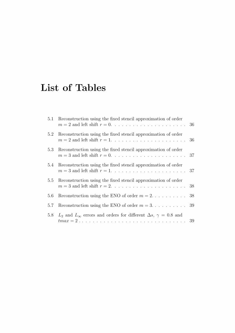
List of Tables
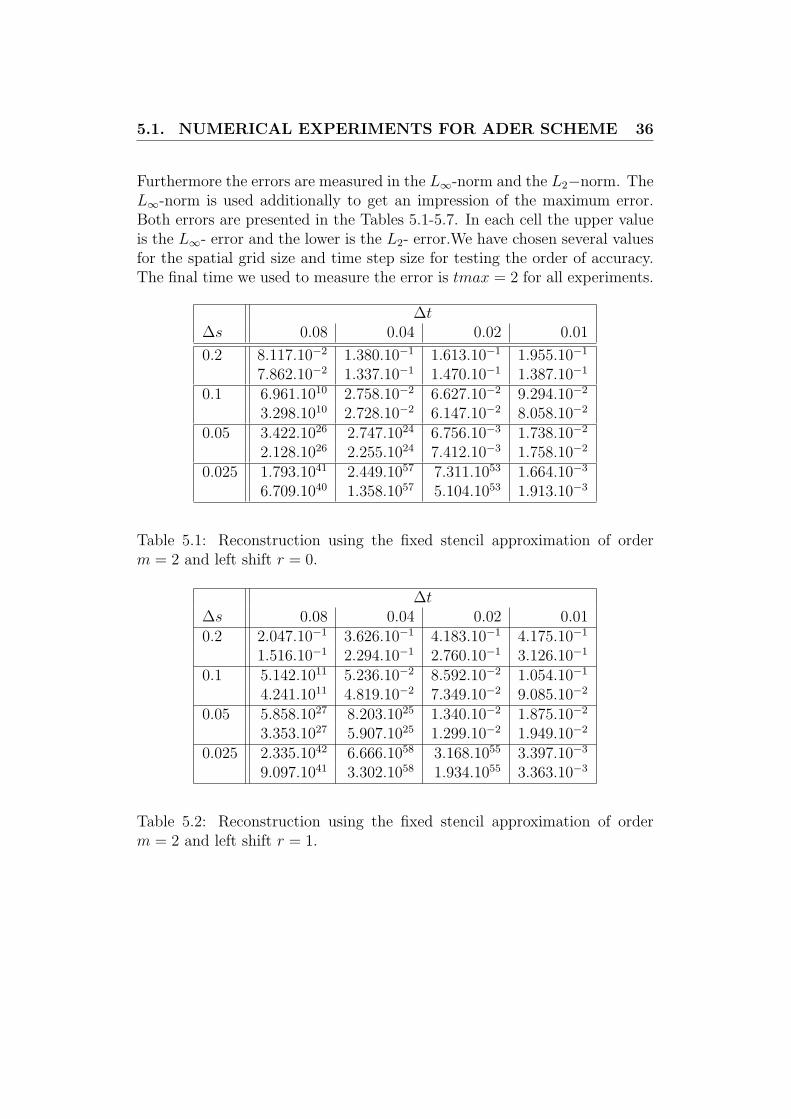
5.1 Reconstruction using the fixed stencil approximation of orderm = 2 and left shift r = 0. . . . . . . . . . . . . . . . . . . . . 36
5.2 Reconstruction using the fixed stencil approximation of orderm = 2 and left shift r = 1. . . . . . . . . . . . . . . . . . . . . 36
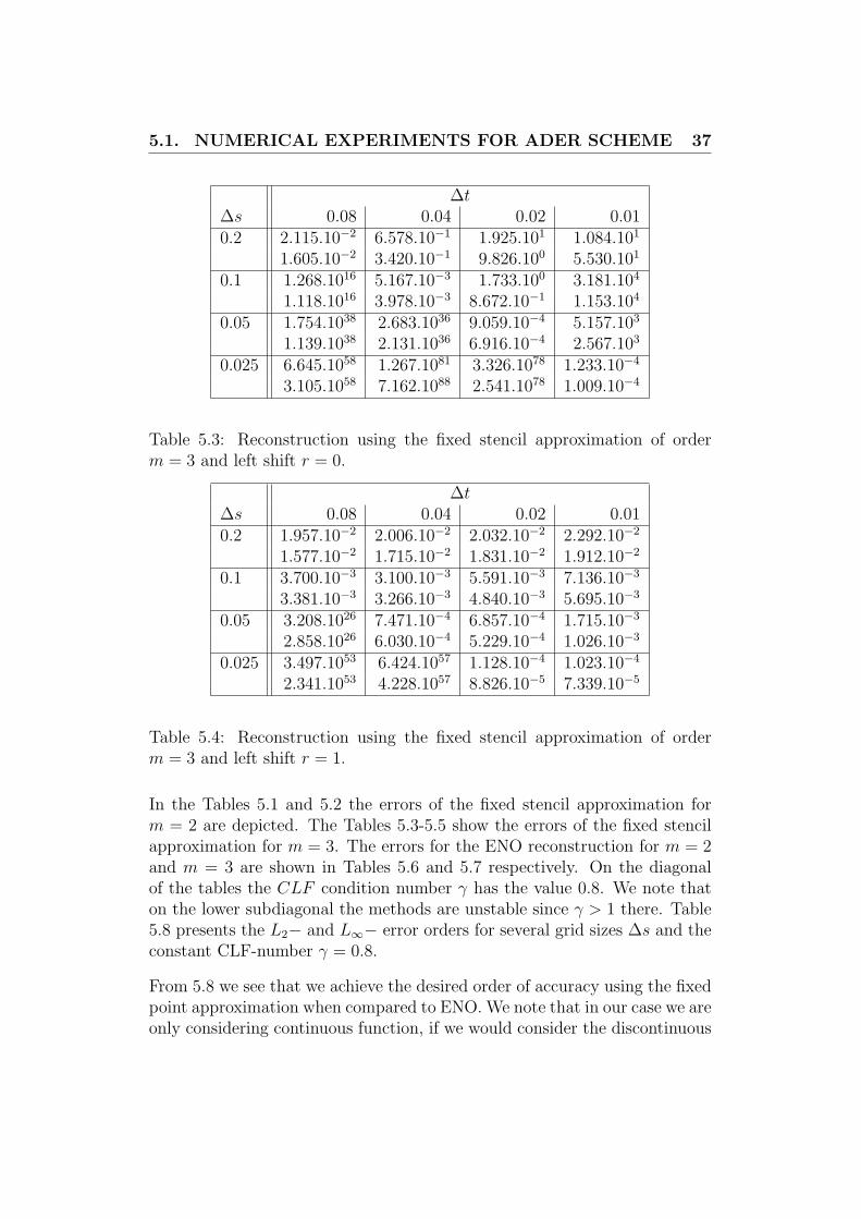
5.3 Reconstruction using the fixed stencil approximation of orderm = 3 and left shift r = 0. . . . . . . . . . . . . . . . . . . . . 37
5.4 Reconstruction using the fixed stencil approximation of orderm = 3 and left shift r = 1. . . . . . . . . . . . . . . . . . . . . 37
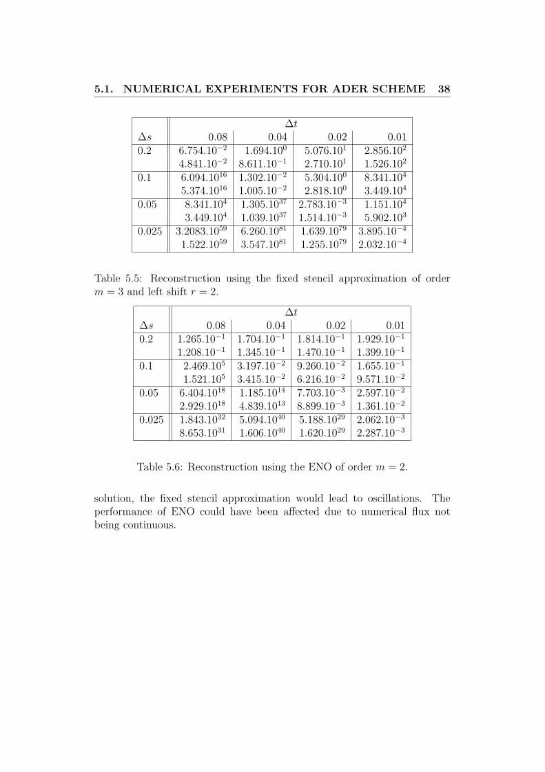
5.5 Reconstruction using the fixed stencil approximation of orderm = 3 and left shift r = 2. . . . . . . . . . . . . . . . . . . . . 38
5.6 Reconstruction using the ENO of order m = 2. . . . . . . . . . 38
5.7 Reconstruction using the ENO of order m = 3. . . . . . . . . . 39
5.8 L2 and L∞ errors and orders for different ∆s, γ = 0.8 andtmax = 2 . . . . . . . . . . . . . . . . . . . . . . . . . . . . . . 39
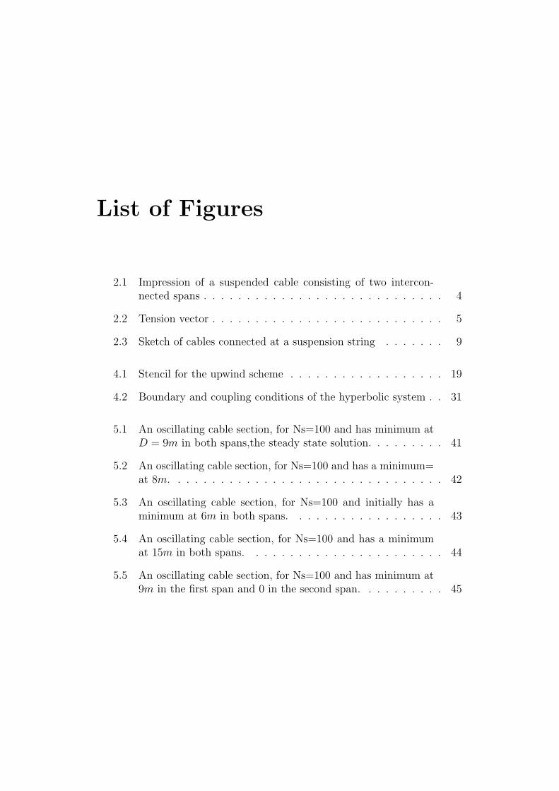
List of Figures
2.1 Impression of a suspended cable consisting of two intercon-nected spans . . . . . . . . . . . . . . . . . . . . . . . . . . . . 4
2.2 Tension vector . . . . . . . . . . . . . . . . . . . . . . . . . . . 5
2.3 Sketch of cables connected at a suspension string . . . . . . . 9
4.1 Stencil for the upwind scheme . . . . . . . . . . . . . . . . . . 19
4.2 Boundary and coupling conditions of the hyperbolic system . . 31
5.1 An oscillating cable section, for Ns=100 and has minimum atD = 9m in both spans,the steady state solution. . . . . . . . . 41
5.2 An oscillating cable section, for Ns=100 and has a minimum=at 8m. . . . . . . . . . . . . . . . . . . . . . . . . . . . . . . . 42
5.3 An oscillating cable section, for Ns=100 and initially has aminimum at 6m in both spans. . . . . . . . . . . . . . . . . . 43
5.4 An oscillating cable section, for Ns=100 and has a minimumat 15m in both spans. . . . . . . . . . . . . . . . . . . . . . . 44
5.5 An oscillating cable section, for Ns=100 and has minimum at9m in the first span and 0 in the second span. . . . . . . . . . 45
ABSTRACT v
Abstract
In this thesis, galloping of overhead transmission lines is studied.This is alow frequency, large amplitude, wind-induced vibrations of both a single anda bundle of overhead transmission lines. The model for this phenomenon isderived from the first principles of Newton’s and Hooke’s laws.
We analyze the model and develop an algorithm for solving the system. Wewill present two numerical schemes, that have been chosen for this task,namely the upwind and ADER schemes. Lastly, conduct several gallopingsimulations under practically relevant conditions.

ACKNOWLEDGEMENTS vi
Acknowledgements
I would like to acknowledge the following people, for without them this studywould not have been completed.
• Dr.Ir. J.H.M. ten Thije Boonkkamp, for supervising this project. Ithank him very much for his support,patience and guidance.
• My friends and colleagues, Cloo, Vryan, Maxim, Henry, Charles, Patri-cio, Marnah, Wanda, Yixin, Eric and Robert. For their support, shar-ing knowledge and the fun we had we together.
• My family, for their love, support, prayers also believing in me.
• The staff of both Eindhoven University of Technology and JohannesKepler University, for their much appreciated assistance for my stay inthese two Universities.
• Last but not least, i would like to acknowledge the European Unionunder the Erusmus Mundus, for their financial support and also for agiving me a chance to study in Europe.
Chapter 1
Introduction
Overhead transmission lines provide the transport highways to move elec-tricity from the generation sources to concentrated areas of customers. Fromthere, the distribution system moves the electricity to where the customeruses it at a business or at home. Unlike other commodities, electricity is gen-erated as it is used and there is very little ability to store it [8]. Because ofthe instantaneous nature of the electric system, constant modifications mustbe made to assure that the generation of power matches the consumption ofpower. The amount of power on a transmission line at any given momentdepends on production and dispatch, customer use, the status of other trans-mission lines and their associated equipment, and even the weather. Thesetransmission lines are cables of aluminium alloy suspended by several towersin a row. The part of the transmission line between two towers is called aspan. The cables are connected to the towers by a freely moveable suspensionstring or insulator, therefore the dynamical motion of neighbouring spans iscoupled.
Companies that supply electricity need to defend against weather-relateddamage and power outages. Ice and snow build-up on high-voltage electricpower lines in moderate to high winds cause large scale mechanical vibrations.This phenomenon of low frequency, large amplitude, wind-induced vibrationsof both a single and a bundle of overhead transmission lines, with a single or afew standing waves per span, is called galloping [3]. Galloping of transmissionlines is a dangerous phenomenon that seriously threatens the security ofpower systems. It is known that galloping causes such serious transmissionproblems as short circuits due to the entanglement of lines, snapping of theline-to-line spacers and the breakage of transmission towers. It is a result
2
of aerodynamic instability of conductors related to many aspects, such asparameters of transmission lines, temperature, speed and direction of wind,shape and position of the attached ice, etc [5]. It has attracted the attentionof many researchers who are attempting to understand and control this costlyvibration. To avoid accidents such as marginal discharge, break or line mixingin regions where galloping is likely to occur, the maximum amplitude of thetransmission lines should be calculated. Some analytical and experimentalmethods have been proposed and implemented in the past years. In general,galloping can roughly be divided into two types, vertical galloping withouttwist and torsional galloping with elliptical vibrating trajectory [5]. Thelatter is a much more complex non-linear problem, related to many aero-dynamic conditions as well as the stiffness of the conductors.
In this thesis we will consider the former. Although both torsional motionand horizontal cable deflection are important for the full problem we assumetorsion to be decoupled from the vertical vibration and the horizontal motionto be negligible. This type of galloping have been mathematically simulatedusing the finite element method [5], but we will derive a suitable algorithmand numerical techniques (ADER and upwind) for the simulation.
The outline of this thesis is as follows.
In Chapter 2, a mathematical model based on first principles of Newton’s andHooke’s law is derived. Asymptotic reduction of the full model, resulting ina systematic model, is discussed [4].
Chapter 3, we come up with a numerical solution procedure by analyzingboth the stationary and time dependent part of the systematic model derivedin the previous chapter. The procedure includes a hyperbolic system whichneeds to be solved.
In chapter 4, we discuss the solution of the hyperbolic system. The upwindand ADER schemes are discussed in detail. The abbreviation ADER standsfor ”Arbitrary high order schemes using DERivatives”. This is a finite volumescheme. In general, we approximate every smooth function to arbitrary highorder of accuracy using its Taylor expansion. Boundary conditions are alsoderived.
In chapter 5, the schemes are implemented. Simulations are conducted usingpractical relevant example parameters from [4]. Numerical results are given.
The last chapter , we summarize the work done, give some conclusive remarksand some ideas for the extension of this work.
Chapter 2
Problem Formulation
In this chapter we will derive a systematic model by asymptotic reductionof the model found in [4] and [3]; details on asymptotic reduction are foundin the same references. We derive the model from the first principles ofNewton’s and Hooke’s laws. Then present a reduced model based on asymp-totic analysis. Last in this chapter we shall discuss boundary and couplingconditions.
2.1 Mathematical model
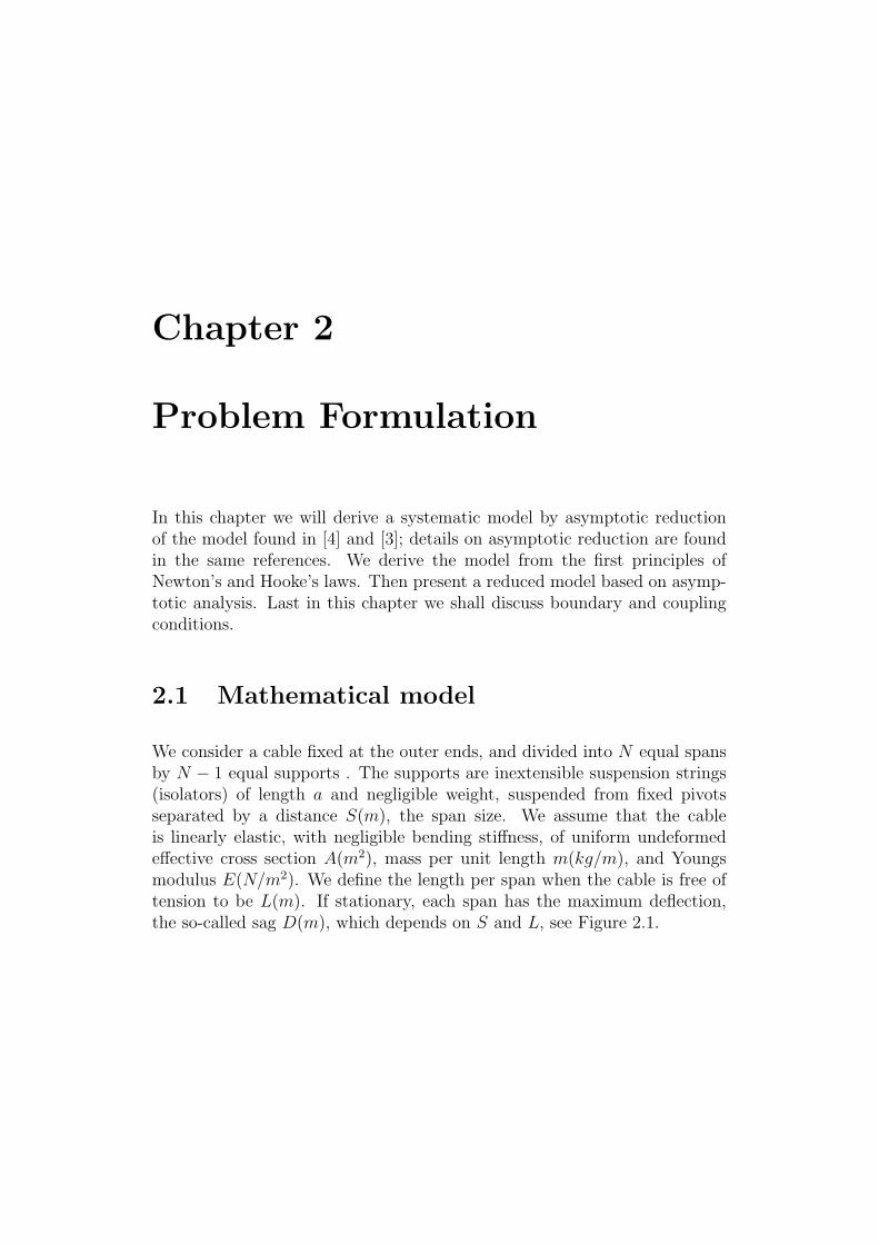
We consider a cable fixed at the outer ends, and divided into N equal spansby N − 1 equal supports . The supports are inextensible suspension strings(isolators) of length a and negligible weight, suspended from fixed pivotsseparated by a distance S(m), the span size. We assume that the cableis linearly elastic, with negligible bending stiffness, of uniform undeformedeffective cross section A(m2), mass per unit length m(kg/m), and Youngsmodulus E(N/m2). We define the length per span when the cable is free oftension to be L(m). If stationary, each span has the maximum deflection,the so-called sag D(m), which depends on S and L, see Figure 2.1.
2.1. MATHEMATICAL MODEL 4
Figure 2.1: Impression of a suspended cable consisting of two interconnectedspans
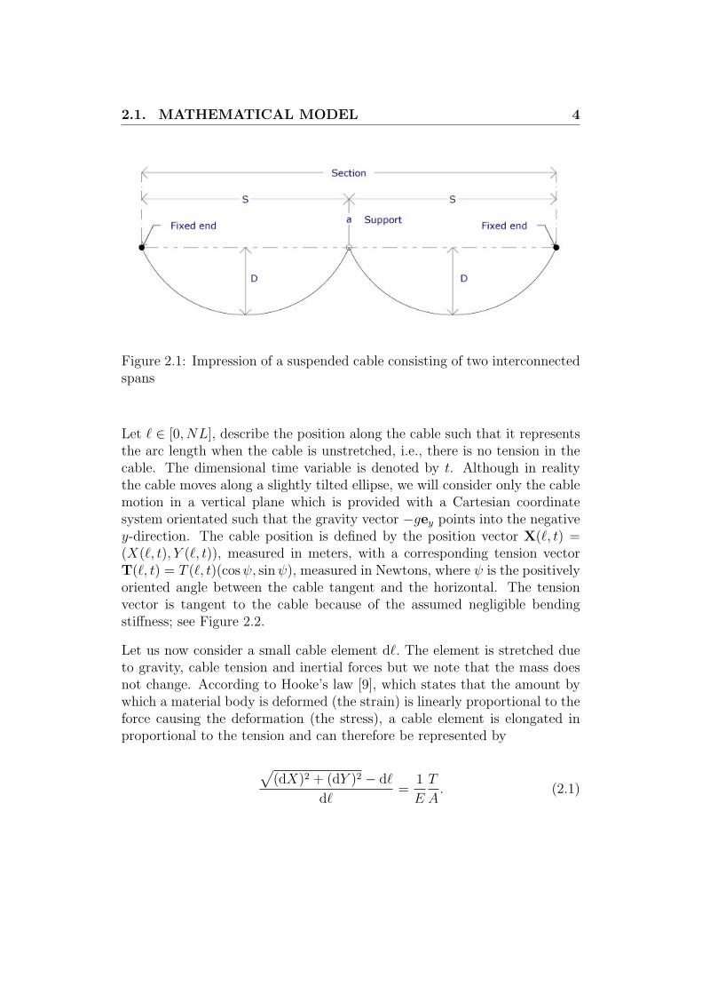
Let ` ∈ [0, NL], describe the position along the cable such that it representsthe arc length when the cable is unstretched, i.e., there is no tension in thecable. The dimensional time variable is denoted by t. Although in realitythe cable moves along a slightly tilted ellipse, we will consider only the cablemotion in a vertical plane which is provided with a Cartesian coordinatesystem orientated such that the gravity vector −gey points into the negativey-direction. The cable position is defined by the position vector X(`, t) =(X(`, t), Y (`, t)), measured in meters, with a corresponding tension vectorT(`, t) = T (`, t)(cosψ, sinψ), measured in Newtons, where ψ is the positivelyoriented angle between the cable tangent and the horizontal. The tensionvector is tangent to the cable because of the assumed negligible bendingstiffness; see Figure 2.2.
Let us now consider a small cable element d`. The element is stretched dueto gravity, cable tension and inertial forces but we note that the mass doesnot change. According to Hooke’s law [9], which states that the amount bywhich a material body is deformed (the strain) is linearly proportional to theforce causing the deformation (the stress), a cable element is elongated inproportional to the tension and can therefore be represented by
√(dX)2 + (dY )2 − d`
d`=
1
E
T
A. (2.1)
2.1. MATHEMATICAL MODEL 5
Figure 2.2: Tension vector
Rearranging terms in equation (2.1), we obtain(∂X
∂`
)2
+
(∂Y
∂`
)2
=
(1 +
T
EA
)2
. (2.2)
.
According to Newton’s second law, the net force on a particle is proportionalto the rate of its linear momentum, usually represented as F = ma. Sincemomentum is a product of mass and velocity, this is given by
∂T
∂`= m
(∂2X
∂t2+ gey
). (2.3)
The x-component of the tension is given by
∂
∂`(Tx) = m
∂2X
∂t2, (2.4)
and along the y-component, since gravitational force is acting, the tension isdescribed by
2.2. REDUCED PROBLEM 6
∂
∂`(Ty) = m
(∂2X
∂t2+ g
), (2.5)
where Tx = T cosψ and Ty = T sinψ . The tension vector is tangent to thecable because of the assumed negligible bending stiffness. From (2.2) it isobvious that
∣∣∣∣∂X∂`∣∣∣∣ = 1 +
T
EA, (2.6)
and therefore we have the sine and cosine of ψ defined by
cosψ =∂X∂`
1 + TEA
, sinψ =∂Y∂`
1 + TEA
. (2.7)
We then substitute (2.7) into (2.4) and (2.5) resulting in the system
∂
∂`
(T
1 + T/EA
∂X
∂`
)= m
∂2X
∂t2, (2.8a)
∂
∂`
(T
1 + T/EA
∂Y
∂`
)= m
∂2Y
∂t2+mg. (2.8b)
The mathematical model is described by (2.2) and (2.8).
2.2 Reduced problem
The type of motion we are interested in allows further reduction of the model.This is motivated by the ratio of sag D, which is the stationary vertical dis-placement and the cable length L. The ratio is known to be small, accordingto [3] it is typically in the order of 1
30. Therefore we have the slenderness,
ε = D/L→ 0
and this is clearly a small parameter problem. This basic small parameter εis used to reduce the general problem to an asymptotic model. Asymptotic
2.2. REDUCED PROBLEM 7
methods are usually most powerful precisely when numerical approaches en-counter their most serious difficulties, such as in cases of small parameters,phenomena on vastly different scales etc. Perturbation / asymptotic analysiscan then provide accurate information in analytic forms which are very wellsuited for both understanding and for further analysis [6].
The longitudinal wave speed is given by cL = (EA/m)12 , and the longitudinal
wave length λL is large compared to the length of the cable L leading to theestimate L/λL = O(ε). The frequency ω is inversely proportional to the wavelength and we have L/λL = ωL/cL = O(ε). We now introduce the referencefrequency ωref = εcL/L. The dimensionless frequency ω∗ and time variablet∗ are given by
ω = ωrefω∗, t = t∗/ωref . (2.9)
We also have that the total vertical non-stationary displacement Y is ofthe order of the sag D,and the transversal wave length λT is of order Lso that Y/L = O(ε) and λT/L = O(1). Clearly, we see that Y scales on
εL. The transversal wave velocity is given by cT = (T/m)12 , thus we have
λT/L = cT/ωL = O(1). This yields that the tension scales on Tref = ε2EA.Putting everything together, we have for ` ∈ the n− th span
` = (n− 1 + s)L, Y (`, t) = εLY ∗(s, t∗;n), T (`, t) = TrefT∗(s, t∗;n),
(2.10)where (∗) are dimensionless variables and where the variable s is a localnondimensional parameter, such that s ∈ [0, 1] parametrizing, the positionwithin a span. We also have to scale X, and we are only interested in thex-displacements that are very small. By substituting the above estimates inequation (2.8b), it transpires that ∂
∂`X = 1+O(ε2), therefore for X from the
n-th span we have
X(`, t) = (n− 1)S + Ls+ ε2LX∗(s, t∗;n). (2.11)
If we substitute the present estimates in (2.8b),we get the term mgL/EAε3
next to terms of order 1,so it is either has to be of order 1 or smaller. Assum-ing that it is smaller, then the stationary solution would be Y = 0 to leadingorder, so D = 0, which contradicts our scaling assumptions. Therefore itfollows that the term is of order 1. We introduce
µ =mgL
8EAε3= O(1) (2.12)
where the factor 8 comes from the assumption that the cable has a ratio ofsag to span of about 1:8 see [7]. For details on asymptotic expansions see [4]and [3].
2.3. BOUNDARY AND COUPLING CONDITIONS 8
Finally, we substitute all the above estimates in the system of equations (2.2)and (2.8). We obtain, under the approximation of small ε, the governingequations [4].
∂T ∗
∂s= 0, (2.13a)
∂
∂s
(T ∗∂Y ∗
∂s
)= 8µ+
∂2Y ∗
∂t∗2, (2.13b)
∂X∗
∂s+
1
2
(∂Y ∗
∂s
)2
= T ∗. (2.13c)
2.3 Boundary and coupling conditions
In this section we derive the boundary and coupling conditions for the modelof two spans (N = 2). We will then scale them using the estimates from theprevious section.
• We have fixed supports at ` = 0 and ` = 2L, therefore we have
X(0, t) = 0, Y (0, t) = 0 (` = 0), (2.14a)
X(2L, t) = 2S Y (2L, t) = 0 (` = 2L). (2.14b)
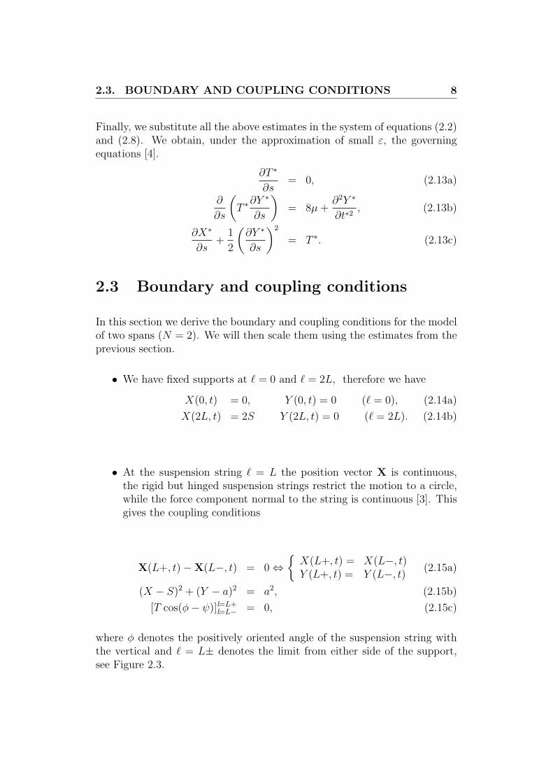
• At the suspension string ` = L the position vector X is continuous,the rigid but hinged suspension strings restrict the motion to a circle,while the force component normal to the string is continuous [3]. Thisgives the coupling conditions
X(L+, t)−X(L−, t) = 0 ⇔X(L+, t) = X(L−, t)Y (L+, t) = Y (L−, t) (2.15a)
(X − S)2 + (Y − a)2 = a2, (2.15b)
[T cos(φ− ψ)]l=L+l=L− = 0, (2.15c)
where φ denotes the positively oriented angle of the suspension string withthe vertical and ` = L± denotes the limit from either side of the support,see Figure 2.3.
2.3. BOUNDARY AND COUPLING CONDITIONS 9
Figure 2.3: Sketch of cables connected at a suspension string
In the first span we have n = 1 and s ∈ [0, 1]. Substituting these into therelations (2.10) and (2.11) we have
` = sL, Y (`, t) = εLY ∗(s, t∗; 1), T (`, t) = TrefT∗(s, t∗; 1),
X(`, t) = Ls+ ε2LX∗(s, t∗; 1).(2.16)
At the first fixed support we have s = 0 and ` = 0, hence we obtain theboundary conditions
X(0, t) = 0 ⇐⇒ ε2LX∗(0, t∗; 1) = 0 ⇐⇒ X∗(0, t∗; 1) = 0, (2.17)
Y (0, t) = 0 ⇐⇒ εLY ∗(0, t∗; 1) = 0 ⇐⇒ Y ∗(0, t∗; 1) = 0. (2.18)
For the second span we have n = 2 and s ∈ [0, 1] and substituting these into(2.10) and (2.11) we have
` = (1 + s)L, Y (`, t) = εLY ∗(s, t∗; 2), T (`, t) = TrefT∗(s, t∗; 2),
X(`, t) = S + Ls+ ε2LX∗(s, t∗; 2).
(2.19)
2.3. BOUNDARY AND COUPLING CONDITIONS 10
In the second span there is a fixed support at the end point, where ` = 2Land s = 1, leading to the boundary conditions
X(2L, t) = 2S ⇐⇒ S + L+ ε2LX∗(1, t∗; 2) = 2S
⇐⇒ X∗(1, t∗; 2) =S − L
ε2L= S0,
Y (2L, t) = 0 ⇐⇒ εLY ∗(1, t∗; 2) = 0 ⇐⇒ Y ∗(1, t∗; 2) = 0.
(2.20)
For the conditions at the suspension string we have for the first span, s = 1and ` = 1 and for the same point on the second span we have s = 0 and` = 2. It is observed that aφ/L = O(ε2), as it is of order of the x-variation,therefore φ = O(ε) [3]. For small ε we obtain the scaled coupling conditions.
From (2.15c) we have
T ∗(1, t∗; 1) = T ∗(0, t∗; 2). (2.21)
We have
Y (L, t) = 0 ⇐⇒ εLY ∗(1, t∗; 1) = εLY ∗(0, t∗; 2) = 0
⇐⇒ Y ∗(1, t∗; 1) = Y ∗(0, t; 2) = 0.(2.22)
For X(L, t) we have the coupling condition
X(L−, t) = X(L+, t) ⇐⇒ L+ ε2LX∗(1, t∗; 1) = S + ε2LX∗(0, t∗; 2) = 0
⇐⇒ X∗(1, t∗; 1) = X∗(0, t∗; 2) + S0.
(2.23)
Chapter 3
Numerical Solution Procedure
In this chapter we will analyze how to solve the governing equations (2.13)incorperating the boundary and the coupling conditions derived in the pre-vious chapter. In practice, the sag D and the span size S are known but thelength of the cable L is unknown and is to be determined. This means thatε and µ are to be determined from the stationary solution. We assume thatall problem parameters are the same for all spans and hence the stationarysolution is periodic in space. This motivates the analysis of a stationary anda nonstationary part. The stationary solution will later be used as the initialcondition for the the nonstationary solution.
3.1 Stationary solution
For the steady part of the problem we will represent the variables with asubscript 0, and then from (2.10) and (2.11) we have
T0(`) = Tref .T∗0 (s;n), X0(`) = (n− 1)S + Ls+ ε2LX∗
0 (s;n),
Y0(`) = εLY ∗0 (s;n).
(3.1)
We then have the governing equations for the stationary state given by
dT ∗0ds
= 0, (3.2a)
T ∗0d2Y ∗
0
d2s= 8µ, (3.2b)
dX∗0
ds+
1
2
(dY ∗
0
ds
)2
= T ∗0 . (3.2c)
3.1. STATIONARY SOLUTION 12
For the first span we have the boundary conditions, Y ∗0 (0; 1) = Y ∗
0 (1; 1) = 0and X∗
0 (0; 1) = 0. Since Y is scaled on the sag D, from symmetry weexpect the location of the maximum deflection half-way, hence we haveY (1
2L) = −D ⇔ Y ∗
0 (12; 1) = −1.To compute Y ∗
0 we integrate twice equation(3.2b) on the interval [0, 1] with respect to s and incoperate the boundaryequations. To find the steady solution of T we substitute the maximumdeflection condition of Y ∗
0 . We obtain
T ∗0 (s; 1) = µ and Y ∗0 (s; 1) = 4s(s− 1). (3.3)
We note that at the suspension spring, s = 1, we do not have a boundarybut a coupling condition which implicitly determines the unknown length L.Therefore, substituting Y ∗
0 into (3.2c), integrate the equation with respect tos and incoperate the boundary condition we obtain
X∗0 (s; 1) = µs− 4
3[(2s− 1)3 + 1]. (3.4)
The distance from the first fixed point to the suspension point is just thespan size S, thus we have
X∗0 (L) = S ⇐⇒ L+ ε2LX∗
0 (1; 1) = S. (3.5)
Since from (3.4) we have X∗0 (1; 1) = µ− 8
3, we now have
X∗0 (L) = S0 ⇐⇒ L2 − SL+D2
(µ− 8
3
)= 0, D = εL. (3.6)
Substituting µ = mgL8EAε3 in (3.6) we obtain the equation which determines the
length L, i.e.,
αL4 + L2 − SL− 8
3D2 = 0 α :=
mg
8EAD. (3.7)
In the second span we have ` = (1 + s)L . For the boundaries we havethe first suspension string s = 0, ` = L and the condition Y0(L) = 0 ⇔Y ∗
0 (0; 2) = 0. At the last fixed support s = 1, ` = 2L we have the boundarycondition Y0(2L) = 0 ⇔ Y ∗
0 (1; 2) = 0. From symmetry we assume again
3.2. NON-STATIONARY SOLUTION 13
that the maximum deflection is halfway the second span, hence we haveY (3
2L) = −D ⇔ Y ∗
0 (12; 2) = −1. We obtain the solutions for the second span
T ∗0 (s; 2) = µ, Y ∗0 (s; 2) = 4s(s−1), X∗
0 (s; 2) = µs−4
3[(2s−1)3+1]. (3.8)
These results show that the solution is indeed periodic and we have the lastboundary condition automatically satisfied, i.e.,
X∗0 (2L) = 2S0 ⇐⇒ X∗
0 (L) = S0. (3.9)
3.2 Non-stationary solution
In this section we will analyze the solution of the time depend part of thegoverning equations. From (2.13a) we have T ∗ = T ∗(t∗) in a single span.Since we have the coupling condition (2.21) we conclude that
T ∗(t∗; 1) = T ∗(t∗; 2) = T ∗(t∗). (3.10)
From (2.13b) we have
T ∗∂2Y ∗
∂s2=∂2Y ∗
∂t2+ 8µ. (3.11)
We define
v :=∂Y ∗
∂t+ 8µt, w :=
∂Y ∗
∂s. (3.12)
We then obtain
∂v
∂t∗=
∂2Y ∗
∂t∗2+ 8µ = T ∗
∂2Y ∗
∂s∗2= T ∗
∂w
∂s(3.13a)
∂w
∂t∗=
∂
∂s
(∂Y ∗
∂t∗
)=
∂
∂s(v − 8µt∗) =
∂v
∂s. (3.13b)
Substituting w into equation (2.13c) we obtain
∂X∗
∂s+
1
2w2 = T ∗. (3.14)
3.2. NON-STATIONARY SOLUTION 14
From (3.13) we have
∂u
∂t+ A.
∂u
∂s= 0, (3.15)
where
u =
(v
w
)A(u) =
(0 −T ∗−1 0
).
Note that since T ∗ = T ∗(t∗), we have A = A(t∗). The matrix A has twodifferent nonzero eigenvalues and two linearly independent eigenvectors. Itthen follows that system (3.15) is diagonalizable and therefore hyperbolic.Numerical methods used to solve this hyperbolic system will the discussed indetail in the next chapter. Y ∗(s, t∗;n) can therefore be computed per spanfrom the solutions w or v by integrating with respect to s equation w = ∂Y ∗
∂s.
From (3.14) we can compute the tension. Integrating equation (3.14) withrespect to s over the first span and incorporating the boundary conditionX∗(0, t∗; 1) = 0 we obtain
T ∗(t∗) = X∗(1, t; 1) +1
2
∫ 1
0
w2(s, t∗; 1)ds > 0. (3.16)
For the second span we apply the same procedure but use the boundarycondition X∗(1, t∗; 2) = S0 and we obtain
T ∗(t∗) = S0 −X∗(0, t; 2) +1
2
∫ 1
0
w2(s, t∗; 2)ds. (3.17)
To find the tension in both spans we add the two relatons (3.16) , (3.17) andapply the coupling condition X∗(1, t∗; 1) − X∗(0, t∗; 2) = S0 and obtain theexpression
T ∗(t∗) = S0 +1
4
∫ 1
0
w2(s, t∗; 1)ds+1
4
∫ 1
0
w2(s, t∗; 2)ds. (3.18)
We then compute X∗(s, t∗;n). We differentiate (3.14) with respect to s andobtain
3.2. NON-STATIONARY SOLUTION 15
∂2X∗
∂s2+ w
∂w
∂s= 0. (3.19)
We solve this system per span and incoperate the boundary conditionsX∗(0, t∗; 1) =0,X∗(1, t∗; 2) = S0 and the coupling condition X∗(1, t∗; 1) = S0 +X∗(0, t∗; 2).
We summarize the procedure discussed above in the form of an algorithm
Algorithm 1 Swinging cables algorithm
1: Compute L from αL4 + L2 − SL− 83D2 = 0 , α := mg
8EAD
compute ε = DL , µ = αL4
D2 , S0 = µ− 83
2: Give initial conditions: X∗0 (s), Y ∗
0 (s), T ∗03: Compute T ∗(0)
T ∗(0) = S0 + 14
∫ 10 w2(s, 0; 1)ds + 1
4
∫ 10 w2(s, 0; 2)ds
4: repeat5: Solve ∂un
∂t∗ + A.∂un∂s = 0 (numerical scheme)
6: Compute Y ∗(s, t∗;n).∂Y ∗
n∂s = wn
Y ∗(0, t∗; 1) = 0, Y ∗(1, t∗; 1) = 0Y ∗(0, t∗; 2) = 0, Y ∗(1, t∗; 2) = 0.
7: Compute T ∗(t∗)T ∗(t∗) = S0 + 1
4
∫ 10 w2(s, t∗; 1)ds + 1
4
∫ 10 w2(s, t∗; 2)ds
8: Solve ∂2X∗n
∂s2 + wn.∂wn∂s = 0
X∗(0, t∗; 1) = 0, X∗(1, t∗; 2) = S0
X∗(1, t∗; 1) = S0 + X∗(0, t∗; 2).9: t∗n = t∗n+1
10: until tmax
Chapter 4
Numerical Solution of theHyperbolic System
In this chapter we present two numerical schemes, viz the upwind and theADER schemes, to solve the linear system of hyperbolic conservation laws.First we will compute the analytical solution of system (3.15). We will thenderive the two numerical schemes and apply the schemes to our problemof interest. Stability for both schemes is investigated. Finally we deriveboundary conditions.
4.1 Analytical solution
Considering the initial value problem
ut + Aus = 0 in R2 × (0, Tmax), (4.1a)
u(s, 0) = υ(s) in R2, (4.1b)
where
u =
(v
w
)A =
(0 −T ∗−1 0
).
4.2. UPWIND SCHEME 17
The matrix A has the eigensystem,
r1 =
(c
1
), r2 =
(−c1
), λ1 = −c < 0, λ2 = c > 0, c =
√T ∗.
(4.2)
Since we have two linear independent eigenvectors, the system (4.1) is diago-nalizable so that A = RΛR−1 where Λ =diag(λ1, λ2) and R = (r1 r2). Wenow introduce the characteristic variable u(s, t) := R−1u(s, t) satisfying thedecoupled system
ut + Λus = 0. (4.3)
We have the characteristic variable u given by u(s, t) = R−1u(s, t) compo-nentwise, we obtain
v =1
2
(vc
+ w), w =
1
2
(−vc
+ w). (4.4)
We find, see [4], v(s, t) = v(s+ ct, 0) and w(s, t) = w(s− ct, 0).
Combining these results with the above relations for the characteristic vari-ables, we obtain the analytic solution,
v(s, t) =1
2
[υ1(s+ ct) + υ1(s− ct) +
c(υ2(s+ ct)− υ2(s− ct))], (4.5a)
w(s, t) =1
2
[1
c
(υ1(s+ ct)− υ1(s− ct)
)+
(υ2(s+ ct) + υ2(s− ct))], (4.5b)
thus the solution u consists of two components, one propagating with velocityλ1 = −c and the other with velocity λ2 = c. Since λ1 < 0, a wave propagatesin the negative x−direction and since λ2 > 0, the other wave propagates inthe positive x−direction.
4.2 Upwind scheme
In order to compute a numerical solution of (3.15), we cover the domainΩ := R× [0,∞) with grid point (sj, t
n), where sj := j∆s for j ∈ Z and tn :=n∆t for n ∈ N with ∆s the spatial grid size and ∆t the time step. We will
4.2. UPWIND SCHEME 18
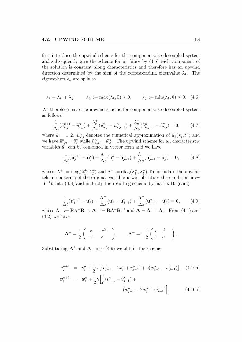
first introduce the upwind scheme for the componentwise decoupled systemand subsequently give the scheme for u. Since by (4.5) each component ofthe solution is constant along characteristics and therefore has an upwinddirection determined by the sign of the corresponding eigenvalue λk. Theeigenvalues λk are split as
λk = λ+k + λ−k , λ+
k := max(λk, 0) ≥ 0, λ−k := min(λk, 0) ≤ 0. (4.6)
We therefore have the upwind scheme for componentwise decoupled systemas follows
1
∆t(un+1
k,j − unk,j) +
λ+k
∆s(un
k,j − unk,j−1) +
λ−k∆s
(unk,j+1 − un
k,j) = 0, (4.7)
where k = 1, 2. unk,j denotes the numerical approximation of uk(sj, t
n) andwe have un
1,k = vnk while un
2,k = wnk . The upwind scheme for all characteristic
variables uk can be combined in vector form and we have
1
∆t(un+1
j − unj ) +
Λ+
∆s(un
j − unj−1) +
Λ−
∆s(un
j+1 − unj ) = 0, (4.8)
where, Λ+ := diag(λ+1 , λ
+2 ) and Λ− := diag(λ−1 , λ
−2 ).To formulate the upwind
scheme in terms of the original variable u we substitute the condition u :=R−1u into (4.8) and multiply the resulting scheme by matrix R giving
1
∆t(un+1
j − unj ) +
A+
∆s(un
j − unj−1) +
A−
∆s(un
j+1 − unj ) = 0, (4.9)
where A+ := RΛ+R−1, A− := RΛ−R−1 and A = A+ +A−. From (4.1) and(4.2) we have
A+ =1
2
(c −c2−1 c
), A− = −1
2
(c c2
1 c
).
Substituting A+ and A− into (4.9) we obtain the scheme
vn+1j = vn
j +1
2γ
[(vn
j+1 − 2vnj + vn
j−1) + c(wnj+1 − wn
j−1)], (4.10a)
wn+1j = wn
j +1
2γ[1
c(vn
j+1 − vnj−1) +
(wnj+1 − 2wn
j + wnj−1)
]. (4.10b)
4.2. UPWIND SCHEME 19
where γ = c∆t∆s
.
The stability of the upwind scheme is ensured if the corresponding scalarupwind schemes for all variables uk are stable. This is shown in details in[4]. This requirement gives the Courant, Friedrichs and Lewy (CFL) stabilitycondition
λ∆t
∆s≤ 1 ⇐⇒ c
∆t
∆s≤ 1, (4.11)
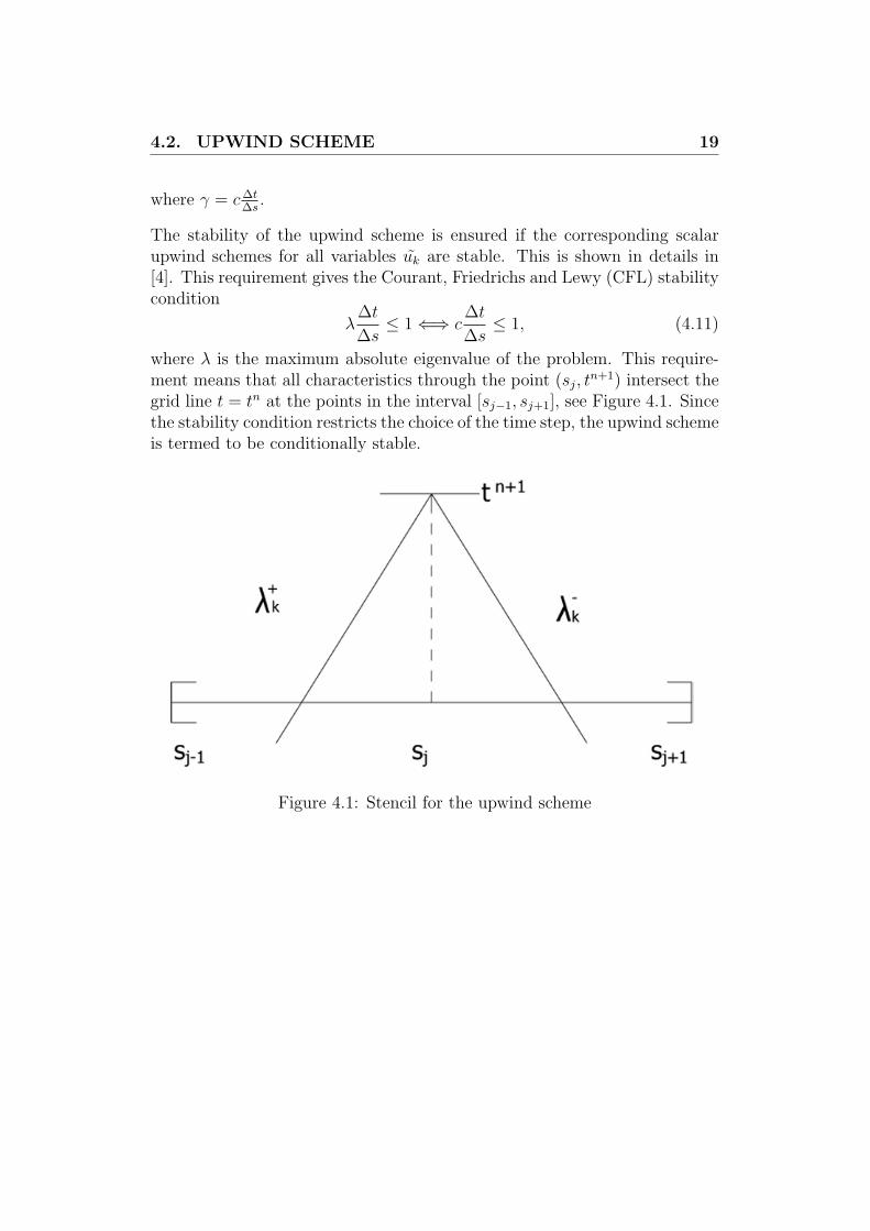
where λ is the maximum absolute eigenvalue of the problem. This require-ment means that all characteristics through the point (sj, t
n+1) intersect thegrid line t = tn at the points in the interval [sj−1, sj+1], see Figure 4.1. Sincethe stability condition restricts the choice of the time step, the upwind schemeis termed to be conditionally stable.
Figure 4.1: Stencil for the upwind scheme
4.3. ADER SCHEMES 20
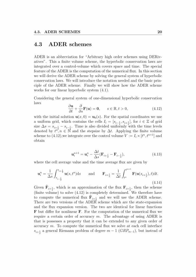
4.3 ADER schemes
ADER is an abbreviation for “Arbitrary high order schemes using DERiv-atives”. This a finite volume scheme, the hyperbolic conservation laws areintegrated over a control-volume which covers space and time. The specialfeature of the ADER is the computation of the numerical flux. In this sectionwe will derive the ADER scheme by solving the general system of hyperbolicconservation laws. We will introduce the notation needed and the basic prin-ciple of the ADER scheme. Finally we will show how the ADER schemeworks for our linear hyperbolic system (4.1).
Considering the general system of one-dimensional hyperbolic conservationlaws
∂u
∂t+
∂
∂sF(u) = 0, s ∈ R, t > 0, (4.12)
with the initial solution u(x, 0) = u0(s). For the spatial coordinates we usea uniform grid, which contains the cells Ii = [si− 1
2, si+ 1
2], for i ∈ Z of grid
size ∆s = si+ 12− si− 1
2. Time is also divided uniformly with the time levels
denoted by tn, n ∈ N and the stepsize by ∆t. Applying the finite volumescheme to (4.12),we integrate over the control volume V := Ii× [tn, tn+1] andobtain
un+1i = un
i −∆t
∆s(Fi+ 1
2− Fi− 1
2), (4.13)
where the cell average value and the time average flux are given by
uni =
1
∆s
∫ si+1
2
si− 1
2
u(s, tn)ds and Fi+ 12
=1
∆t
∫ tn+1
tnF(u(si+ 1
2), t)dt.
(4.14)Given Fi+ 1
2, which is an approximation of the flux Fi+ 1
2, then the scheme
(finite volume) to solve (4.12) is completely determined. We therefore haveto compute the numerical flux Fi+ 1
2and we will use the ADER scheme.
There are two versions of the ADER scheme which are the state-expansionand the flux expansion version. The two are identical for linear functionsF but differ for nonlinear F. For the computation of the numerical flux werequire a certain order of accuracy m. The advantage of using ADER isthat is possesses a property that it can be extended to any given order ofaccuracy m. To compute the numerical flux we solve at each cell interfacesi+ 1
2a general Riemann problem of degree m− 1 (GRPm−1), but instead of
4.3. ADER SCHEMES 21
a piecewise constant initial conditions we have polynomials of degree m− 1on the left and right side of the discontinuity. Thus we have to solve
∂tu + ∂sF(u) = 0, s ∈ R, t > tn
u(s, t) =
uL(s) := pi(s), s < si+ 1
2
uR(s) := pi+1(s), s > si+ 12
(4.15)
The initial conditions uL(s) and uR(s) are computed using some constructionmethod described briefly later. To obtain a scheme of order m, we expressthe approximate solution of (GRPm−1) (4.15) as a Taylor series expansion intime at the cell interface. Defining τ = t− tn, we have
u(si+ 12, t) = u(si+ 1
2, tn+) +
m−1∑k=1
[∂
(k)t u(si+ 1
2, tn+)
] τ k
k!+O(τm), (4.16)
where ∂kt u(s, t) := ∂k
∂tku(s, t). The leading term u(si+ 1
2, tn+) is the Godunov
state solution of the conventional Riemann problem (with piecewise constantdata) GRP0
∂tu + ∂sF(u) = 0, s ∈ R, t > tn
u(s, t) =
uL(si+ 1
2), s < si+ 1
2
uR(si+ 12), s > si+ 1
2.
(4.17)
We now have to compute ∂(k)t u(si+ 1
2, tn+) for the remaining m − 1 terms.
Since the derivatives with respect to time are usually not available at eachcell interface si+ 1
2, we use a method that is based on the representation of the
time derivatives in terms of spatial derivatives of u; for details see [1]. We
therefore compute the spatial derivatives.We define u(k) = ∂(k)s u the k − th
spatial derivative. Taking the derivative of (4.12) with respect to s we obtain
0 = ∂s(∂tu) + ∂s[∂sF(u)]
= ∂tu(1) + F′(u)∂su
(1) + ∂s
(F′(u)
)u(1). (4.18)
4.3. ADER SCHEMES 22
Hence, u(1) is determined from ∂tu(1) + F′(u)∂su
(1) = −∂s
(F′(u)
)u(1). Re-
peating the procedure of taking the derivative with respect to s of (4.12) ktimes, we obtain
∂tu(k) + F′(u)∂su
(k) = Gk(u,u(1), ...,u(k)). (4.19)
The function Gk is an algebraic function of u and all its derivative are ofdegree less than or equal to k. For the linear system the function Gk = 0.We only need u(k) at the first instant interaction of the left and right intialstates. According to [1] it is justified to neglect the source terms. The systemis linearized hence we obtain the state variable u(k) by solving the RP0
∂tu(k) + F′(u(si+ 1
2, tn+))∂su
(k) = 0, s ∈ R, t > tn
u(s, tn) =
u
(k)L = ∂
(k)s uL(si+ 1
2), s < si+ 1
2
u(k)R = ∂
(k)s uR(si+ 1
2), s > si+ 1
2.
(4.20)
We note that, to obtain the state variables for the numerical flux we solve onenonlinear and m− 1 linear Riemann-problems. We express time derivativesin terms of space derivatives. After computing all spatial derivatives we setup the Taylor expansion (4.16) as follows
u(si+ 12, τ) = C0 + C1τ + ...Cm−1
τm−1
(m− 1)!. (4.21)
Ck are constant vectors obtained from the Cauchy-Kovalevskaya method[14] together with spatial derivatives computed from (4.20). Hence (4.21)approximates the value of u at the interface si+ 1
2with an order of accuracy
m in time.
Finally we compute the numerical flux Fi+ 12. This is where the two ver-
sions of ADER differ. For the state expansion method, the numerical fluxis computed by using the approximate quadrature rules. Applying Gaussianquadrature we obtain
Fi+ 12
=Kα∑α=0
F(u(si+ 12, γα∆t))ωα, (4.22)
where γα and ωα are properly chosen nodes and weights. Kα is the numberof nodes and has to be chosen accordingly to the order m. For the flux
4.3. ADER SCHEMES 23
expansion version, we consider the Taylor series expansion of the physicalflux with respect to time
F(si+ 12, t) = F(si+ 1
2, tn+)
m−1∑k=1
[∂(k)t F(si+ 1
2, tn+)]
τ k
k!+O(τm). (4.23)
Hence, from (4.14) and (4.23), omitting the term O(τm), the numerical fluxis given by
Fi+ 12
= F(si+ 12, tn+) +
m−1∑k=1
[∂(k)t F(si+ 1
2, tn+)]
∆tk
(k + 1)!. (4.24)
The first term of (4.24) accounts for the interaction of the initial data and itis approximated using monotone flux functions like Godunov, Lax-Friedrich,etc [1]. in terms of the left and right cell boundary values. The other termsare computed by taking the derivatives of F(u) with respect to time t up toorder m− 1. These two methods (4.22) and (4.24) are the same for a linearsystem since we can compute the integral (4.14) exactly.
4.3.1 ADER scheme for a linear system
In this section we apply the scheme derived in the previous section to thelinear system of conservation laws (3.15). Since both the state-expansionand the flux-expansion versions of ADER give the same results for the linearsystem we can choose either one of the two. We will therefore use the state-expansion. To compute the numerical flux we first solve the appropriateGeneralized Riemann problem GRPm−1. Its solution will then be expressedin terms of a Taylor series expansion, see(4.16). We then express the time
derivatives in terms of spatial derivatives ∂(k)s u(s, t). The first derivative
∂tu(s, t) follow from the conservation law
∂tu(s, t) = −A∂su(s, t). (4.25)
Taking the time derivative of (4.25), we obtain the second time derivative
∂(2)t u(s, t) = A2∂
(2)s u(s, t). Therefore, we can conclude by induction for gen-
eral k, we have the k − th time derivative
∂(k)t u(s, t) = (−A)k∂(k)
s u(s, t). (4.26)
4.3. ADER SCHEMES 24
The determination of the time derivatives of u reduces to the estimation ofthe spatial derivatives u(k)(s, t). The spatial states u(k)(s, t) are associatedto the conventional Riemann problem RP0
∂tu + A∂su(k) = 0, s ∈ R, t > tn
u(k)(s, tn) =
u
(k)L = u
(k)L (si+ 1
2), s < si+ 1
2
u(k)R = u
(k)R (si+ 1
2), s > si+ 1
2.
(4.27a)
The sought particular values of the solutions to GRP0 is u(k)(si+ 12, tn+), the
so-called the Godunov state. Using (4.26), the Taylor expansion reads
u(si+ 12, t) = u(si+ 1
2, tn+) +
m−1∑k=1
[(−A)ku(k)(si+ 1
2, tn+)
] τ k
k!+O(τm), (4.28)
and hence the flux is computed from (4.14),i.e.,
Fi+ 12
= Au(si+ 12, tn+) +
m−1∑k=1
[(−A)ku(k)(si+ 1
2, tn+)
] ∆tk
(k + 1)!. (4.29)
The cell average value un+1i in the next step is given by (4.13). Finally we
have to compute the solutions of GRP0u(k)(s, τ). We are interested in the
Godunov state u(k)(si+ 12, tn+). For the linear system (4.1) the solution can
be expressed explicitly. We therefore express the solution of (4.27) in termsof eigenvectors (4.2), i.e;
u(k)i (s, t) =
2∑j=1
u(k)j,i (s, t)rj, (4.30)
with scalar functions u(k)j,i (s, t) to be determined later. The double notation
j, i is emphasized since u(k)j,i differ for every i. The initial functions uL(s)
and uR(s) can also decoupled since υ1 and υ2 are linearly independent. Weobtain
u(k)L (si+ 1
2) =
2∑j=1
α(k)j,i υj and u
(k)R (si+ 1
2) =
2∑j=1
β(k)j,i υj, (4.31)

4.3. ADER SCHEMES 25
with suitable constants α(k)j,i and β
(k)j,i . We are now considering the decoupled
system of equations. Using knowledge of the linear advection equation, thescalar function are given by
u(k)j,i (s− si+ 1
2, t) = u
(k)j,i (s− si+ 1
2− λj(t− tn), tn)
=
α
(k)j,i ,
s−si+1
2
t−tn< λj,
β(k)j,i ,
s−si+1
2
t−tn> λj.
(4.32)
The values u(k)j,i (si+ 1
2, tn+) correspond to the condition
u(k)j,i (si+ 1
2, tn+) =
α
(k)j,i , 0 < λj,
β(k)j,i , 0 > λj.
(4.33)
We note that, since the first eigenvalue is negative and the second one ispositive, the Godunov state using (4.32) and (4.33) is given by
u(k)i (si+ 1
2, tn+) = β
(k)1,i r1 + α
(k)2,i r2. (4.34)
4.3.2 Reconstruction and initial data
In this section we will show the basic issues, which are important for a numer-ical implementation of the ADER scheme. We will also present the structureof the conventional Riemann problems, i.e., we will state the initial datafor arbitrary expansion index m. In this thesis we will concentrate on thecases m = 2 and m = 3 for the fixed stencil approximation and the ENO-reconstruction.
The initial polynomials uL(s) and uR(s) of the GRP (m − 1) are computedusing the same construction methods. The technique is to construct the cellinterface values of a function using given cell average values. Hence, givenall cell averages un
i at time tn we should be able to construct the cell bound-ary values u±
i+ 12
with an accuracy of order m. These methods include the
essentially nonoscillatory (ENO), weighted ENO (WENO) reconstructions
4.3. ADER SCHEMES 26
etc. Form [2],[10], [11] or [12] we obtain for each interface two reconstructedvalues, u+
i+ 12
and u−i+ 1
2
.These are the cell boundary reconstructions at si+ 12
of
u when using a reconstruction stencil based on the i − th cell (denoted by-) and the i+ 1− th cell (denoted by +). For smooth functions these valuesare equal but they differ at discontinuities. We additionally get two recon-struction polynomials which provide the cell boundary values, which are ofdegree m− 1. These polynomials are used to set up the initial conditions of(4.17). The polynomial obtained by reconstruction based on the i − th cellcorresponds to uL(s) while the one based on the i + 1− th cell correspondsto uR(s).
Fixed stencil approximation uses a fixed (defined by the left shift r, which isfixed for all cells) stencil Sr(i) for each cell Ii of length m. We have
Sr(i) = Ii−r, ..., Ii, ..., Ii+m−r−1 (4.35)
to determine pi(s). For each cell we obtain from the reconstruction an inter-polation polynomial polynomial pi,r(s) of degree m − 1, which provides thecell interface values of the function u at si+ 1
2and si− 1
2with an m-th order
accuracy. These polynomials are used to set up the conventional Riemannproblem RP0, which have to be solved to get the solution to the GRPm−1. Wethen have the RP0 for the cell interface si+ 1
2, arbitrary order k = 0, ...,m− 1
and time tn as
∂tu(k) + A∂su
(k) = 0, s ∈ R, t > tn
u(k)(s, tn) =
u
(k)L = p
(k)i,r (si+ 1
2), s < si+ 1
2
u(k)R = p
(k)i+1,r(si+ 1
2), s > si+ 1
2.
(4.36)
We now present the formulas for the initial values u(k)L and u
(k)R at an ar-
bitrary cell interface si+ 12. We note that these values differ in every time
step n and therefore have to be calculated at each time step from the givenapproximation un
i .
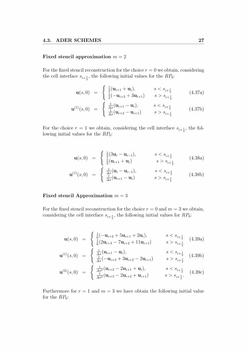
4.3. ADER SCHEMES 27
Fixed stencil approximation m = 2
For the fixed stencil reconstruction for the choice r = 0 we obtain, consideringthe cell interface si+ 1
2, the following initial values for the RP0:
u(s, 0) =
12(ui+1 + ui), s < si+ 1
212(−ui+2 + 3ui+1) s > si+ 1
2
(4.37a)
u(1)(s, 0) =
1
∆s(ui+1 − ui), s < si+ 1
21
∆s(ui+2 − ui+1) s > si+ 1
2
(4.37b)
For the choice r = 1 we obtain, considering the cell interface si+ 12, the fol-
lowing initial values for the RP0:
u(s, 0) =
12(3ui − ui−1), s < si+ 1
212(ui+1 + ui) s > si+ 1
2
(4.38a)
u(1)(s, 0) =
1
∆s(ui − ui−1), s < si+ 1
21
∆s(ui+1 − ui) s > si+ 1
2
(4.38b)
Fixed stencil Approximation m = 3
For the fixed stencil reconstruction for the choice r = 0 and m = 3 we obtain,considering the cell interface si+ 1
2, the following initial values for RP0:
u(s, 0) =
16(−ui+2 + 5ui+1 + 2ui), s < si+ 1
216(2ui+3 − 7ui+2 + 11ui+1) s > si+ 1
2
(4.39a)
u(1)(s, 0) =
1
∆s(ui+1 − ui), s < si+ 1
21
∆s(−ui+3 + 3ui+2 − 2ui+1) s > si+ 1
2
(4.39b)
u(2)(s, 0) =
1
∆s2 (ui+2 − 2ui+1 + ui), s < si+ 12
1∆s2 (ui+3 − 2ui+2 + ui+1) s > si+ 1
2.
(4.39c)
Furthermore for r = 1 and m = 3 we have obtain the following initial valuefor the RP0:
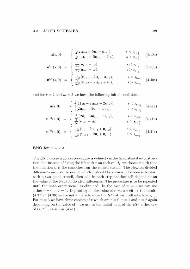
4.3. ADER SCHEMES 28
u(s, 0) =
16(2ui+1 + 5ui − ui−1), s < si+ 1
216(−ui+2 + 5ui+1 + 2ui), s > si+ 1
2
(4.40a)
u(1)(s, 0) =
1
∆s(ui+1 − ui), s < si+ 1
21
∆s(ui+1 − ui), s > si+ 1
2
(4.40b)
u(2)(s, 0) =
1
∆s2 (ui+1 − 2ui + ui−1), s < si+ 12
1∆s2 (ui+2 − 2ui+1 + ui), s > si+ 1
2
(4.40c)
and for r = 2 and m = 3 we have the following initial conditions:
u(s, 0) =
16(11ui − 7ui−1 + 2ui−2), s < si+ 1
216(2ui+1 + 5ui − ui−1), s > si+ 1
2
(4.41a)
u(1)(s, 0) =
1
∆s(2ui − 3ui−1 + ui−2), s < si+ 1
21
∆s(ui+1 − ui), s > si+ 1
2
(4.41b)
u(2)(s, 0) =
1
∆s2 (ui − 2ui−1 + ui−2), s < si+ 12
1∆s2 (ui+1 − 2ui + ui−1), s > si+ 1
2
(4.41c)
ENO for m = 2, 3
The ENO reconstruction procedure is defined via the fixed stencil reconstruc-tion, but instead of fixing the left shift r on each cell Ii, we choose r such thatthe function u is the smoothest on the chosen stencil. The Newton divideddifferences are used to decide which r should be chosen. The idea is to startwith a two point stencil, then add in each step another cell depending onthe value of the Newton divided differences. The procedure is to be repeateduntil the m-th order stencil is obtained. In the case of m = 2 we can useeither r = 0 or r = 1. Depending on the value of r we use either the results(4.37) or (4.38) as the initial data to solve the RP0 at each cell interface si+ 1
2.
For m = 3 we have three choices of r which are r = 0, r = 1 and r = 2 againdepending on the value of r we use as the initial data of the RP0 either oneof (4.39) , (4.40) or (4.41).
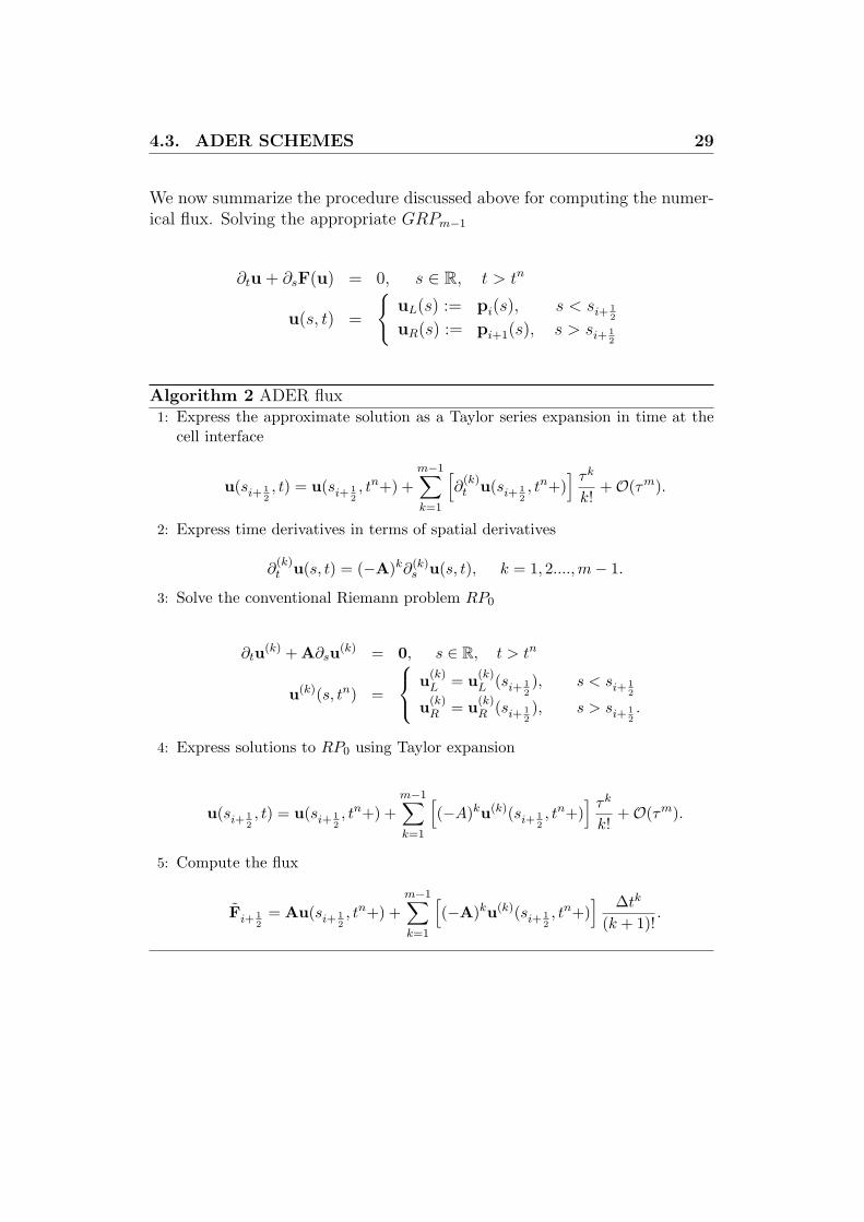
4.3. ADER SCHEMES 29
We now summarize the procedure discussed above for computing the numer-ical flux. Solving the appropriate GRPm−1
∂tu + ∂sF(u) = 0, s ∈ R, t > tn
u(s, t) =
uL(s) := pi(s), s < si+ 1
2
uR(s) := pi+1(s), s > si+ 12
Algorithm 2 ADER flux1: Express the approximate solution as a Taylor series expansion in time at the
cell interface
u(si+ 12, t) = u(si+ 1
2, tn+) +
m−1∑k=1
[∂
(k)t u(si+ 1
2, tn+)
] τk
k!+O(τm).
2: Express time derivatives in terms of spatial derivatives
∂(k)t u(s, t) = (−A)k∂(k)
s u(s, t), k = 1, 2...., m− 1.
3: Solve the conventional Riemann problem RP0
∂tu(k) + A∂su(k) = 0, s ∈ R, t > tn
u(k)(s, tn) =
u(k)L = u(k)
L (si+ 12), s < si+ 1
2
u(k)R = u(k)
R (si+ 12), s > si+ 1
2.
4: Express solutions to RP0 using Taylor expansion
u(si+ 12, t) = u(si+ 1
2, tn+) +
m−1∑k=1
[(−A)ku(k)(si+ 1
2, tn+)
] τk
k!+O(τm).
5: Compute the flux
Fi+ 12
= Au(si+ 12, tn+) +
m−1∑k=1
[(−A)ku(k)(si+ 1
2, tn+)
] ∆tk
(k + 1)!.
4.4. NUMERICAL BOUNDARY CONDITIONS 30
4.3.3 Stability analysis
Investigating the stability of the ADER schemes is complicated, and becomesmore complicated to analyze for higher m. Choosing the ENO/WENO re-constructions we would have to distinguish a lot of different cases, sincedifferent left-shifts r are used for different cells Ii and hence different com-binations have to be investigated. Investigating the stability using the fixedstencil reconstruction for m = 2 and r = 0. Considering the linear advectionequation
∂t + a∂su = 0, s ∈ R, t > 0, a ∈ R. (4.42)
Where u is uniquely determined by (4.42) and the initial condition u(s, 0) =u0(s), s ∈ R. We assume that a > 0 hence the result is right moving wave.This gives the stability condition
γ ≤ 1, (4.43)
where γ = a∆t∆s
, see [12] for full derivation. Subsequently, investigating thestability using the fixed stencil reconstruction for m = 2 and r = 1. Con-sidering the advection equation (4.42) and assuming now that a < 0. Weobtain the stability condition
−γ ≤ 2. (4.44)
We use the above conditions to investigate the stability of the decoupledsystem. Making use of the characteristic decomposition presented in thissection,we choose different reconstruction methods for the two independentequations.We consider the fixed stencil approximation and for the left movingwave r = 0 and r = 1 for the right moving wave. From the stability conditionsabove, we obtained the CLF- condition |γ| ≤ 2. Therefore, we obtain therestriction
γ = λ∆t
∆s≤ 2, (4.45)
where λ is the maximum absolute eigenvalue of the considered problem.
4.4 Numerical boundary conditions
In this section we will discuss and derive the boundary conditions and thecoupling conditions for the hyperbolic system (3.15). Our two span modelhas two boundaries at j = 1 and j = 2N−1, the coupling condition at j = Nas show in Figure 4.2.
4.4. NUMERICAL BOUNDARY CONDITIONS 31
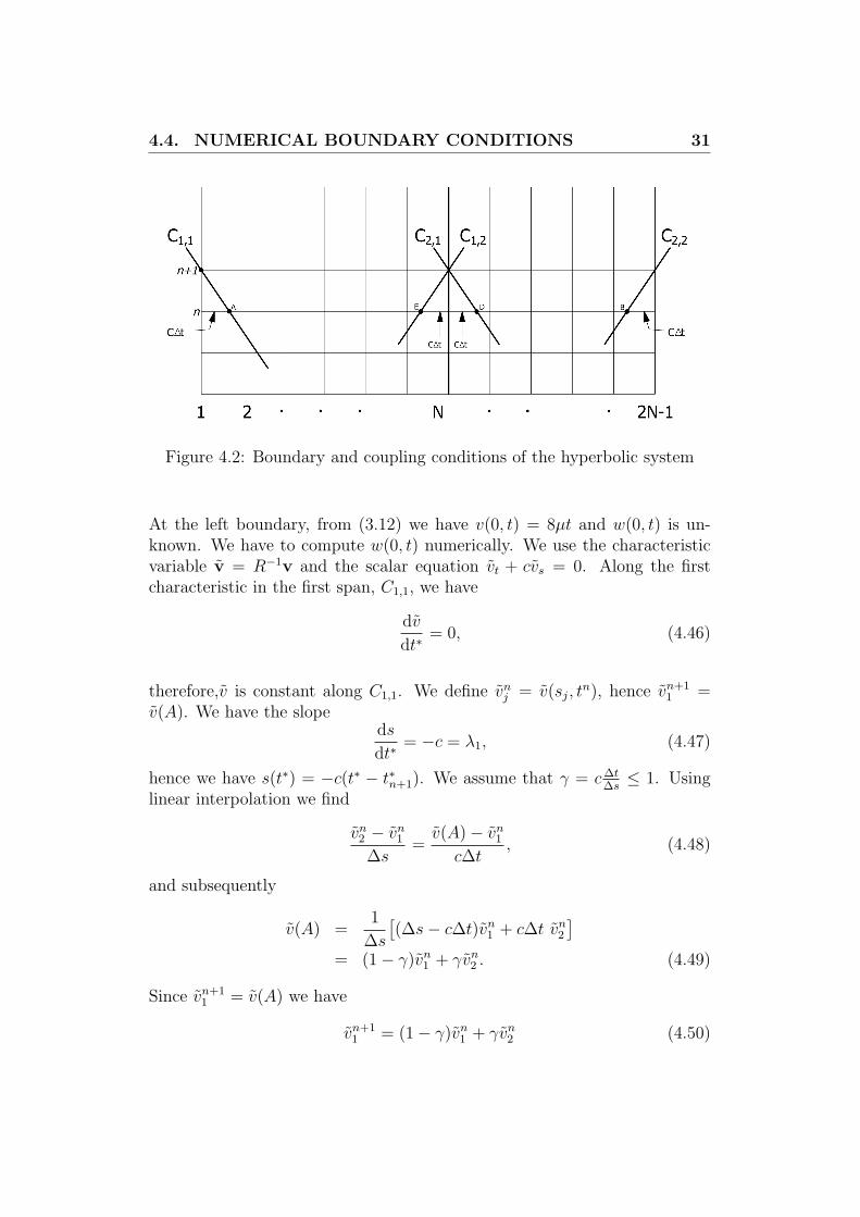
Figure 4.2: Boundary and coupling conditions of the hyperbolic system
At the left boundary, from (3.12) we have v(0, t) = 8µt and w(0, t) is un-known. We have to compute w(0, t) numerically. We use the characteristicvariable v = R−1v and the scalar equation vt + cvs = 0. Along the firstcharacteristic in the first span, C1,1, we have
dv
dt∗= 0, (4.46)
therefore,v is constant along C1,1. We define vnj = v(sj, t
n), hence vn+11 =
v(A). We have the slopeds
dt∗= −c = λ1, (4.47)
hence we have s(t∗) = −c(t∗ − t∗n+1). We assume that γ = c∆t∆s≤ 1. Using
linear interpolation we find
vn2 − vn
1
∆s=v(A)− vn
1
c∆t, (4.48)
and subsequently
v(A) =1
∆s
[(∆s− c∆t)vn
1 + c∆t vn2
]= (1− γ)vn
1 + γvn2 . (4.49)
Since vn+11 = v(A) we have
vn+11 = (1− γ)vn
1 + γvn2 (4.50)
4.4. NUMERICAL BOUNDARY CONDITIONS 32
This is just the upwind scheme for vt + cvs = 0.
From (4.4) we have
v =1
2
(vc
+ w)
=⇒ w = 2v − v
c. (4.51)
Thus we have the boundary conditions;
vn2 =
1
2
(1
cvn
2 + wn2
).
vn+11 = 8µt∗n+1.
wn+11 = 2vn+1
1 − 1
cvn+1
1 .
At the right boundary, from equation (3.12) we have v(S2N−1, t) = 8µt andw(S2N−1, t) has to be computed numerically. We have on C2,2
ds
dt∗= c = λ2, (4.52)
hence we have s(t∗) = 1 + c(t∗ − t∗n+1). Since
dw
dt∗= 0, (4.53)
this means that w is constant along the characteristic C2,2 hence wn+12N−1 =
w(B).
Assuming that γ = c∆t∆s≤ 1, and using linear interpolation we find
wn2N−1 − wn
2N−2
∆s=w2N−1 − w(B)
c∆t, (4.54)
and subsequently
w(B) =1
∆s
[c∆t wn
2N−2 + (∆s− c∆t)wn2N−1
]= γwn
2N−2 + (1− γ)wn2N−1. (4.55)
Since wn+12N−1 = w(B) we have
wn+12N−1 = γwn
2N−2 + (1− γ)wn2N−1. (4.56)
4.4. NUMERICAL BOUNDARY CONDITIONS 33
From (4.4) we have
w =1
2
[−vc
+ w
]=⇒ w = 2w +
v
c. (4.57)
Thus, we have
wn2N−1 =
1
2
(−1
cvn
2N−1 + wn2N−1
).
vn+12N−1 = 8µt∗n+1.
wn+12N−1 = 2wn+1
2N−1 +1
cvn+1
2N−1.
We now consider the coupling condition occurring at j = N . We have from(3.12) that v(1, t∗; 1) = v(0, t∗; 2) = 8µt∗. Along the characteristic C1,2 wehave
ds
dt∗= c =⇒ s(t∗) = 1 + c(t∗ − t∗n+1). (4.58)
Since dwdt
= 0, it implies that w is constant along the characteristic C1,2.Therefore wn+1
N = w(E). Assuming that γ = c∆t∆s
< 1 and using interpolationwe obtain
w(E) = γwnN−1 + (1− γ)wn
N . (4.59)
Hence we havewn+1
N = γwnN−1 + (1− γ)wn
N . (4.60)
Thus;
wnN =
1
2
(−1
cvn
N + wnN
).
vn+1N = 8µt∗n+1.
wn+1N = 2wn+1
N +1
cvn+1
N .
Similarly along C2,1, we have
ds
dt∗= −c =⇒ s(t∗) = −c(t∗ − t∗n+1). (4.61)
Since dv2
dt= 0, it implies that v is constant along C2,1. Therefore vn+1
N =v(D). Assuming that γ = c∆t
∆s< 1 and using interpolation we obtain
v(D) = (1− γ)vnN + γvn
N+1. (4.62)
4.4. NUMERICAL BOUNDARY CONDITIONS 34
Thus;
vnN =
1
2
(1
cvn
N + wnN
).
vn+1N = 8µt∗n+1.
wn+1N = 2vn+1
N − 1
cvn+1
N .
Chapter 5
Numerical Results
In this chapter, we illustrate the performance of the schemes presented in thisthesis. We will first present numerical results and analysis of the accuracyof the ADER scheme for solving the hyperbolic system (3.15). Next we willpresent the simulation results of galloping transmission lines for the upwindscheme.
5.1 Numerical experiments for ADER scheme
In this section we perform numerical tests and measure the error with respectto the given analytical solution (4.5). We are expecting an error of the orderm for constant CLF number, which is defined by
γ = c∆t
∆s,
For our experiments we choose T ∗ = 4, therefore we get c = 2. Thus, the ratiobetween the step size ∆t and the grid size ∆s has to be a constant in orderto obtain the desired order of accuracy m. The linear stability condition,mentioned in [1], is the CLF condition γ ≤ 1. All tests are performed usingthe initial condition,
u0(s) =
(sin πs
cos πs
).
5.1. NUMERICAL EXPERIMENTS FOR ADER SCHEME 36
Furthermore the errors are measured in the L∞-norm and the L2−norm. TheL∞-norm is used additionally to get an impression of the maximum error.Both errors are presented in the Tables 5.1-5.7. In each cell the upper valueis the L∞- error and the lower is the L2- error.We have chosen several valuesfor the spatial grid size and time step size for testing the order of accuracy.The final time we used to measure the error is tmax = 2 for all experiments.
∆t∆s 0.08 0.04 0.02 0.01
0.2 8.117.10−2 1.380.10−1 1.613.10−1 1.955.10−1
7.862.10−2 1.337.10−1 1.470.10−1 1.387.10−1
0.1 6.961.1010 2.758.10−2 6.627.10−2 9.294.10−2
3.298.1010 2.728.10−2 6.147.10−2 8.058.10−2
0.05 3.422.1026 2.747.1024 6.756.10−3 1.738.10−2
2.128.1026 2.255.1024 7.412.10−3 1.758.10−2
0.025 1.793.1041 2.449.1057 7.311.1053 1.664.10−3
6.709.1040 1.358.1057 5.104.1053 1.913.10−3
Table 5.1: Reconstruction using the fixed stencil approximation of orderm = 2 and left shift r = 0.
∆t∆s 0.08 0.04 0.02 0.010.2 2.047.10−1 3.626.10−1 4.183.10−1 4.175.10−1
1.516.10−1 2.294.10−1 2.760.10−1 3.126.10−1
0.1 5.142.1011 5.236.10−2 8.592.10−2 1.054.10−1
4.241.1011 4.819.10−2 7.349.10−2 9.085.10−2
0.05 5.858.1027 8.203.1025 1.340.10−2 1.875.10−2
3.353.1027 5.907.1025 1.299.10−2 1.949.10−2
0.025 2.335.1042 6.666.1058 3.168.1055 3.397.10−3
9.097.1041 3.302.1058 1.934.1055 3.363.10−3
Table 5.2: Reconstruction using the fixed stencil approximation of orderm = 2 and left shift r = 1.
5.1. NUMERICAL EXPERIMENTS FOR ADER SCHEME 37
∆t∆s 0.08 0.04 0.02 0.010.2 2.115.10−2 6.578.10−1 1.925.101 1.084.101
1.605.10−2 3.420.10−1 9.826.100 5.530.101
0.1 1.268.1016 5.167.10−3 1.733.100 3.181.104
1.118.1016 3.978.10−3 8.672.10−1 1.153.104
0.05 1.754.1038 2.683.1036 9.059.10−4 5.157.103
1.139.1038 2.131.1036 6.916.10−4 2.567.103
0.025 6.645.1058 1.267.1081 3.326.1078 1.233.10−4
3.105.1058 7.162.1088 2.541.1078 1.009.10−4
Table 5.3: Reconstruction using the fixed stencil approximation of orderm = 3 and left shift r = 0.
∆t∆s 0.08 0.04 0.02 0.010.2 1.957.10−2 2.006.10−2 2.032.10−2 2.292.10−2
1.577.10−2 1.715.10−2 1.831.10−2 1.912.10−2
0.1 3.700.10−3 3.100.10−3 5.591.10−3 7.136.10−3
3.381.10−3 3.266.10−3 4.840.10−3 5.695.10−3
0.05 3.208.1026 7.471.10−4 6.857.10−4 1.715.10−3
2.858.1026 6.030.10−4 5.229.10−4 1.026.10−3
0.025 3.497.1053 6.424.1057 1.128.10−4 1.023.10−4
2.341.1053 4.228.1057 8.826.10−5 7.339.10−5
Table 5.4: Reconstruction using the fixed stencil approximation of orderm = 3 and left shift r = 1.
In the Tables 5.1 and 5.2 the errors of the fixed stencil approximation form = 2 are depicted. The Tables 5.3-5.5 show the errors of the fixed stencilapproximation for m = 3. The errors for the ENO reconstruction for m = 2and m = 3 are shown in Tables 5.6 and 5.7 respectively. On the diagonalof the tables the CLF condition number γ has the value 0.8. We note thaton the lower subdiagonal the methods are unstable since γ > 1 there. Table5.8 presents the L2− and L∞− error orders for several grid sizes ∆s and theconstant CLF-number γ = 0.8.
From 5.8 we see that we achieve the desired order of accuracy using the fixedpoint approximation when compared to ENO. We note that in our case we areonly considering continuous function, if we would consider the discontinuous
5.1. NUMERICAL EXPERIMENTS FOR ADER SCHEME 38
∆t∆s 0.08 0.04 0.02 0.010.2 6.754.10−2 1.694.100 5.076.101 2.856.102
4.841.10−2 8.611.10−1 2.710.101 1.526.102
0.1 6.094.1016 1.302.10−2 5.304.100 8.341.104
5.374.1016 1.005.10−2 2.818.100 3.449.104
0.05 8.341.104 1.305.1037 2.783.10−3 1.151.104
3.449.104 1.039.1037 1.514.10−3 5.902.103
0.025 3.2083.1059 6.260.1081 1.639.1079 3.895.10−4
1.522.1059 3.547.1081 1.255.1079 2.032.10−4
Table 5.5: Reconstruction using the fixed stencil approximation of orderm = 3 and left shift r = 2.
∆t∆s 0.08 0.04 0.02 0.010.2 1.265.10−1 1.704.10−1 1.814.10−1 1.929.10−1
1.208.10−1 1.345.10−1 1.470.10−1 1.399.10−1
0.1 2.469.105 3.197.10−2 9.260.10−2 1.655.10−1
1.521.105 3.415.10−2 6.216.10−2 9.571.10−2
0.05 6.404.1018 1.185.1014 7.703.10−3 2.597.10−2
2.929.1018 4.839.1013 8.899.10−3 1.361.10−2
0.025 1.843.1032 5.094.1040 5.188.1029 2.062.10−3
8.653.1031 1.606.1040 1.620.1029 2.287.10−3
Table 5.6: Reconstruction using the ENO of order m = 2.
solution, the fixed stencil approximation would lead to oscillations. Theperformance of ENO could have been affected due to numerical flux notbeing continuous.
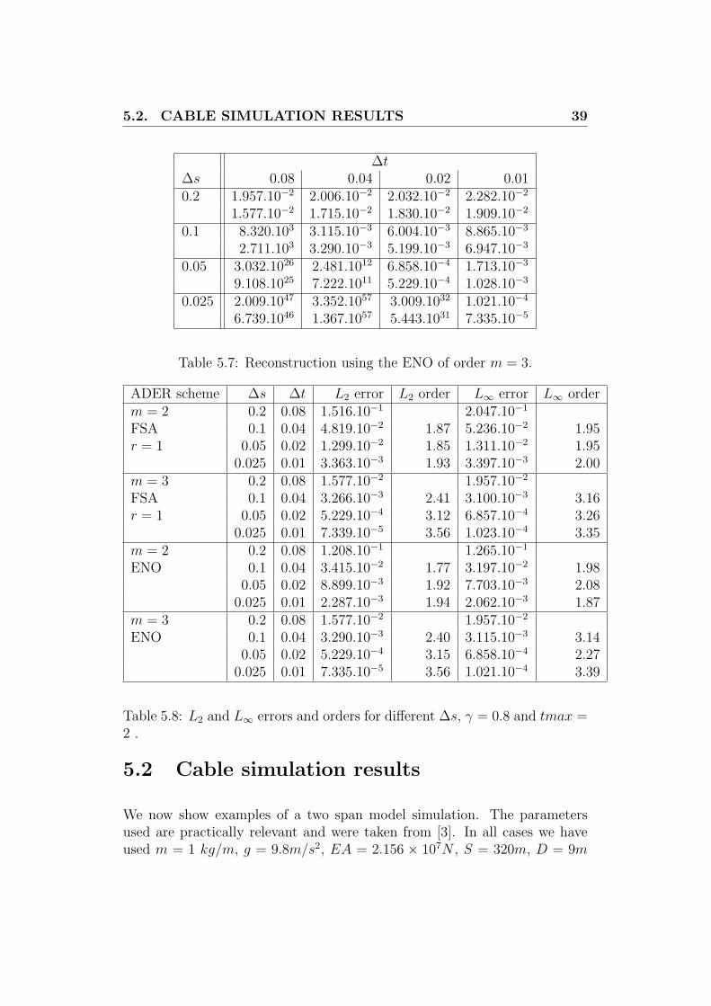
5.2. CABLE SIMULATION RESULTS 39
∆t∆s 0.08 0.04 0.02 0.010.2 1.957.10−2 2.006.10−2 2.032.10−2 2.282.10−2
1.577.10−2 1.715.10−2 1.830.10−2 1.909.10−2
0.1 8.320.103 3.115.10−3 6.004.10−3 8.865.10−3
2.711.103 3.290.10−3 5.199.10−3 6.947.10−3
0.05 3.032.1026 2.481.1012 6.858.10−4 1.713.10−3
9.108.1025 7.222.1011 5.229.10−4 1.028.10−3
0.025 2.009.1047 3.352.1057 3.009.1032 1.021.10−4
6.739.1046 1.367.1057 5.443.1031 7.335.10−5
Table 5.7: Reconstruction using the ENO of order m = 3.
ADER scheme ∆s ∆t L2 error L2 order L∞ error L∞ orderm = 2 0.2 0.08 1.516.10−1 2.047.10−1
FSA 0.1 0.04 4.819.10−2 1.87 5.236.10−2 1.95r = 1 0.05 0.02 1.299.10−2 1.85 1.311.10−2 1.95
0.025 0.01 3.363.10−3 1.93 3.397.10−3 2.00m = 3 0.2 0.08 1.577.10−2 1.957.10−2
FSA 0.1 0.04 3.266.10−3 2.41 3.100.10−3 3.16r = 1 0.05 0.02 5.229.10−4 3.12 6.857.10−4 3.26
0.025 0.01 7.339.10−5 3.56 1.023.10−4 3.35m = 2 0.2 0.08 1.208.10−1 1.265.10−1
ENO 0.1 0.04 3.415.10−2 1.77 3.197.10−2 1.980.05 0.02 8.899.10−3 1.92 7.703.10−3 2.08
0.025 0.01 2.287.10−3 1.94 2.062.10−3 1.87m = 3 0.2 0.08 1.577.10−2 1.957.10−2
ENO 0.1 0.04 3.290.10−3 2.40 3.115.10−3 3.140.05 0.02 5.229.10−4 3.15 6.858.10−4 2.27
0.025 0.01 7.335.10−5 3.56 1.021.10−4 3.39
Table 5.8: L2 and L∞ errors and orders for different ∆s, γ = 0.8 and tmax =2 .
5.2 Cable simulation results
We now show examples of a two span model simulation. The parametersused are practically relevant and were taken from [3]. In all cases we haveused m = 1 kg/m, g = 9.8m/s2, EA = 2.156 × 10⁷N , S = 320m, D = 9m
5.2. CABLE SIMULATION RESULTS 40
and time step ∆t = 10−3 for grid sizes ∆s = 0.01 and initial positions of thecable. The final time used is tmax = 10. For all the experiments the upwindscheme was used.
In the first simulation, we present the initial the position of the cable, thatis the steady state of the cable. We then multiply the the initial conditionsof the steady solution by several factors to change the initial position of thecable for simulations. The results below show the initial position of the cable,the vertical displacement of the cable and the tension against time in eachsimulation.
5.2. CABLE SIMULATION RESULTS 41
(a) Initial position of the cable
(b) Vertical displacement of the cable
(c) Tension against time
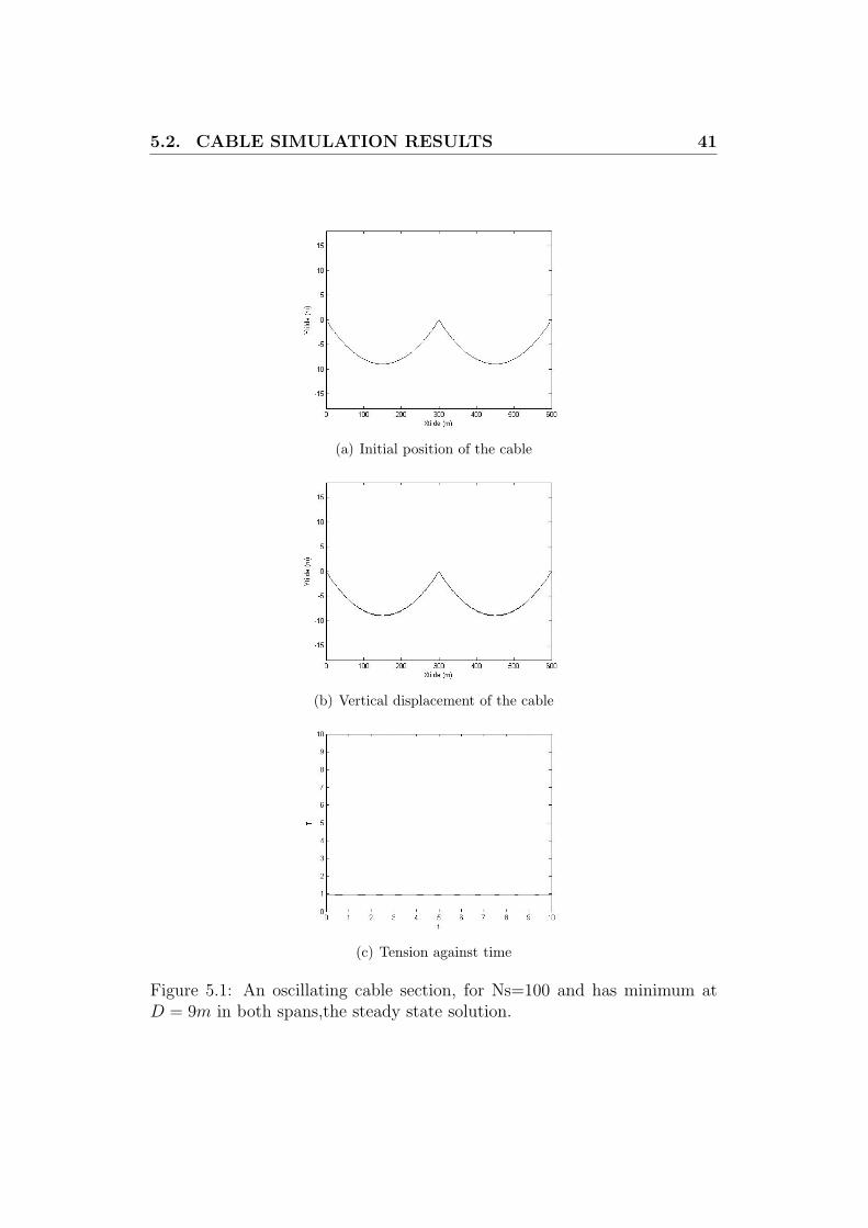
Figure 5.1: An oscillating cable section, for Ns=100 and has minimum atD = 9m in both spans,the steady state solution.
5.2. CABLE SIMULATION RESULTS 42
(a) Initial position of the cable (b) Displacement of the cable att = 0.1
(c) Displacement of the cable att = 0.4
(d) Displacement of the cable att = 1
(e) Displacement of the cable att = 10
(f) Tension against time
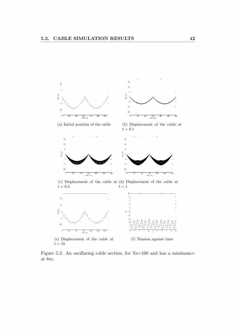
Figure 5.2: An oscillating cable section, for Ns=100 and has a minimum=at 8m.
5.2. CABLE SIMULATION RESULTS 43
(a) Initial position of the cable (b) Vertical displacement of thecable at t = 0.2
(c) Vertical displacement of the ca-ble at t = 0.7
(d) Vertical displacement of thecable at t = 1.2
(e) Vertical displacement of the ca-ble at t = 10
(f) Tension against time
Figure 5.3: An oscillating cable section, for Ns=100 and initially has a min-imum at 6m in both spans.
5.2. CABLE SIMULATION RESULTS 44
(a) Initial position of the cable (b) Vertical displacement of thecable at t = 0.1
(c) Vertical displacement of the ca-ble at t = 0.4
(d) Vertical displacement of thecable at t = 1
(e) Vertical displacement of the ca-ble at t = 10
(f) Tension against time
Figure 5.4: An oscillating cable section, for Ns=100 and has a minimum at15m in both spans.
5.2. CABLE SIMULATION RESULTS 45
(a) Initial position of the cable (b) Vertical displacement of thecable at t = 0.1
(c) Vertical displacement of the ca-ble at t = 0.8
(d) Vertical displacement of thecable at t = 1
(e) Vertical displacement of the ca-ble at t = 10
(f) Tension against time
Figure 5.5: An oscillating cable section, for Ns=100 and has minimum at 9min the first span and 0 in the second span.
5.2. CABLE SIMULATION RESULTS 46
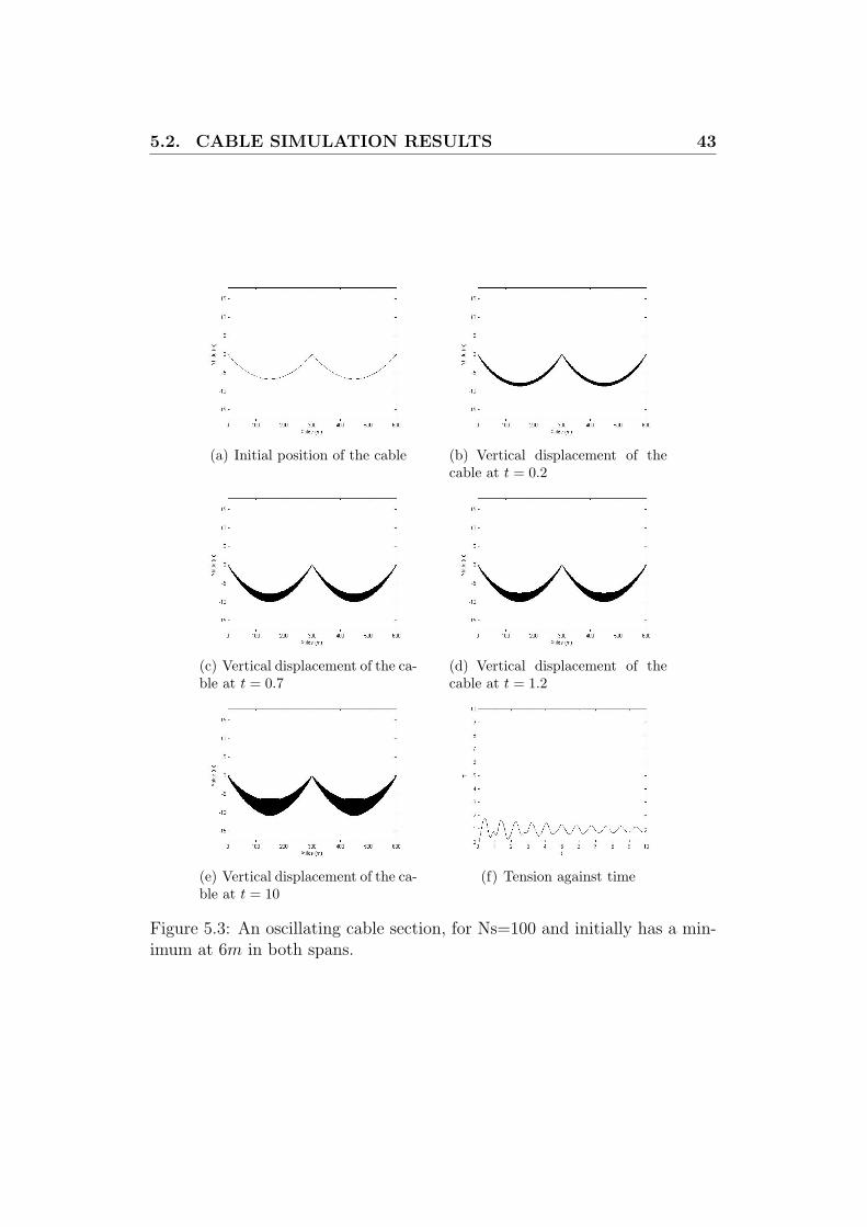
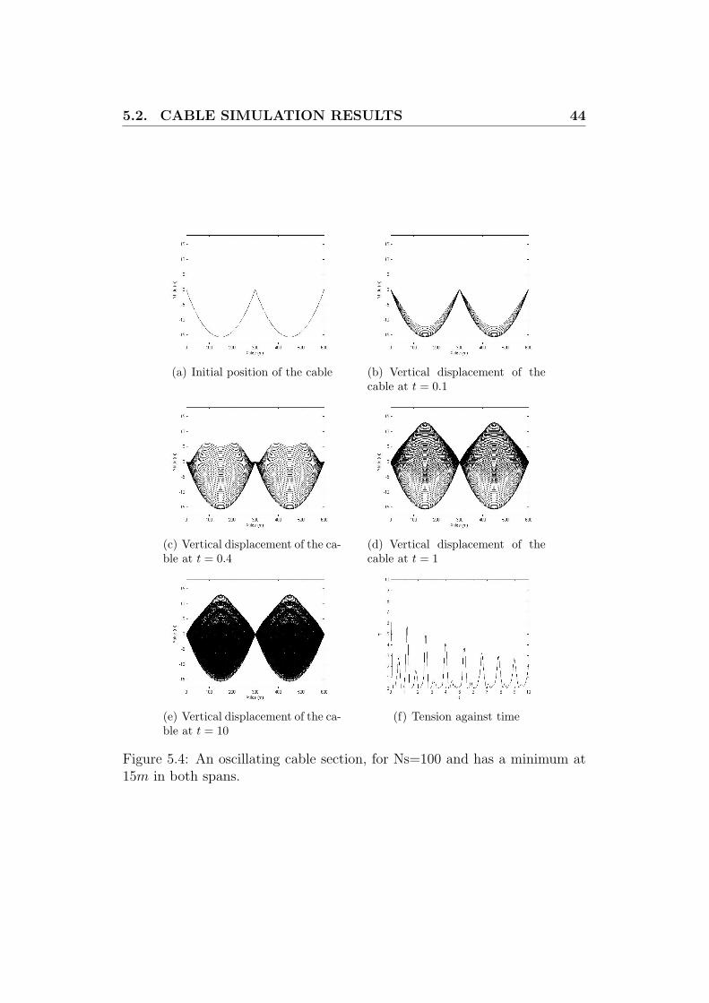
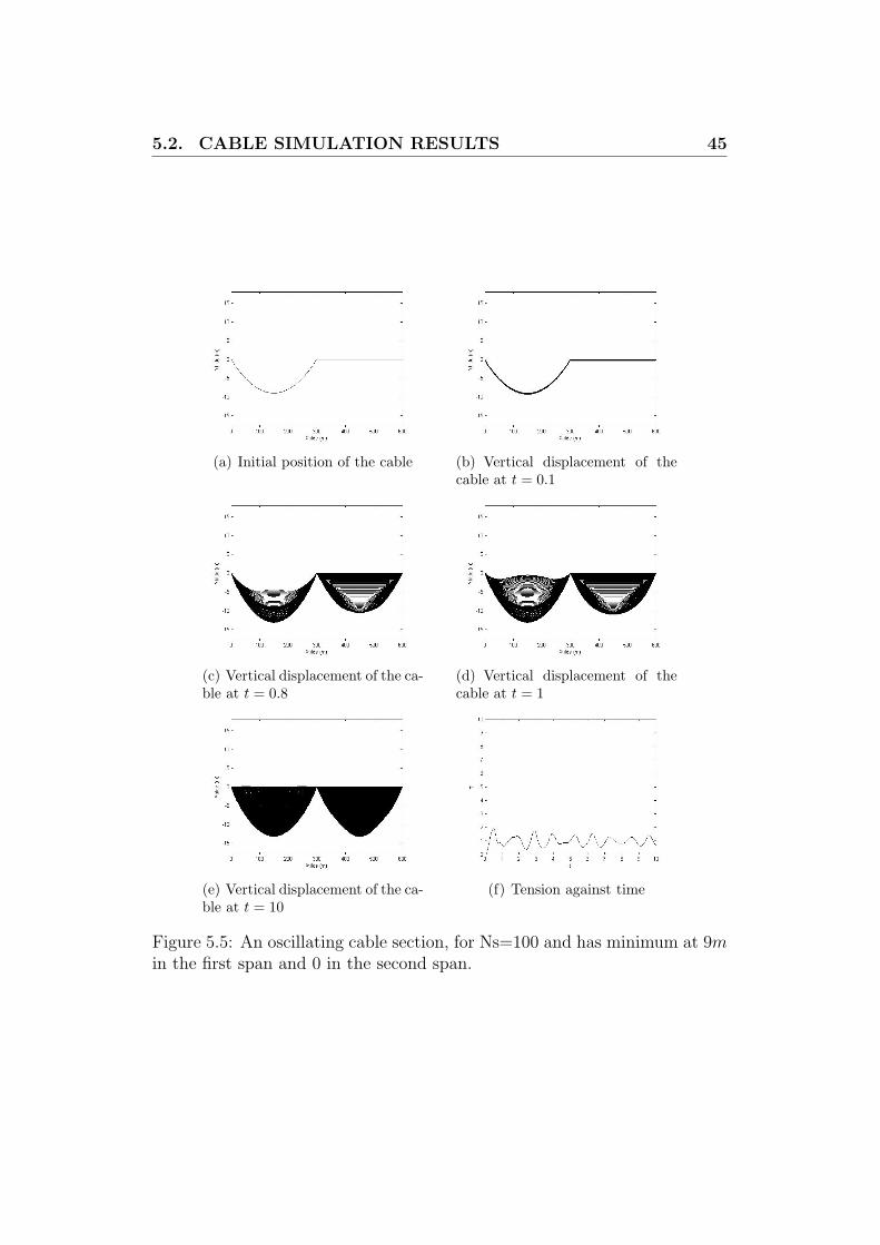
The first case Figure 5.1, we have a steady solution. Tension is constantthroughout, this is expected because the cable is stationary. In the secondcase, the initial conditions of a steady state are changed such that the cableis raised up such that it has a minimum at 8m. When released the cablefalls down first and oscillate up and down. The results are shown in Figure5.2. In the first subfigure the initial position of the cable is shown, the nextone shows the vertical displacement of the cable as it oscillates and the lastfigure shows tension variation in time. For the third case we repeat thesame procedure but with the minimum is at 6m and for the fourth case theminimum is at 15m. In last case we change the initial position only on thesecond span such that minimum of the cable in the second span is at 0.When released, on the second span the cable falls down and the motion istransferred to the first span. This is expected as we have middle point is notfixed, we have coupling conditions.
The motion of the cable seems to be symmetric for the first four tests, butthats not the case for the last test. The last test clearly shows the decouplinggalloping as the motion is transferred from span to another. The tension ischanging per unit time when the cable vibrates, this is expected because asthe cable displacement changes the tension is also affected. From analysis ofthe system we expect tension to be greater than zero, and this is the casewith our results. The length of the cable, L, does not change throughout thecomputation.
Chapter 6
Conclusion andRecommendations
The problem of galloping transmission lines was simulated. The model wasfirst derived from first principles of Newton’s and Hooke’s laws. Asymptoticanalysis was used to reduce the problem, by exploiting the geometrical thick-ness and relative elasticity, resulting in a system of equations to be solvednumerically. Practically relevant parameter were used to simulate the mo-tion of the cable in Matlab. Two schemes, the upwind and ADER, wereimplemented. Although the ADER schemes showed more accurate and sta-ble results when solving linear hyperbolic conservation laws, it is complicatedto implement the scheme to solve the system. This could be due to the factthat the tension is changing per time step, hence the matrix is not fixed.Therefore several tests were conducted using the upwind scheme. The mo-tion is symmetric when the same initial conditions are set on both spans.For the case where different initial conditions were set per span, the motionwas seen to be asymmetric then tends to be symmetric after some time.
The results we obtained do not clarify the characteristics of the galloping phe-nomenon, which could be used to prevent galloping. Therefore the followingare possible suggestions for the extension of the work.
• Propose various external driving forces that improve the model.
• Derive ADER schemes for a non-fixed matrix
• Formulate and simulate the related problem for motion of the cable inthree dimensions.

48
• Conduct several galloping simulations under various analytical condi-tions.
Bibliography
[1] E. F. Toro and V.A. Titarev, TVD Fluxes for the High-Order ADERSchemes, Journal of Scientific Computing, 24 (2005), no. 3, 285–309.
[2] B. Cockburn, C. Johnson, C.W. Shu, and E.Tadmor, Advanced Numer-ical Approximation of Nonlinear Hyperbolic Equations., Lecture Notesin Mathematics, Springer, Italy, 5(4) (1997), 325434.
[3] Sjoerd W. Rienstra, Nonlinear Free Vibration of Coupled Spans of Over-head Transmission Lines, Proceedings of the Third European Confer-ence on Mathematics in Industry 27-31 (1988), 133–144.
[4] R.M.M Mattheij, S.W Rienstra and J.H.M ten Boonkkamp, Partial Dif-ferential Equations : Modelling, Analysis, Computation, Philadephia :SIAM, (2005).
[5] J. H. Zhang, Y. H. Shi and G. X. Liu., Simulation of Transmission LineGalloping Using Finite Element Method IEE 2nd International Confer-ence on Advances in Power System Control,Operation and Management,Hong Kong 1993, 644–648.
[6] C.M Bender and S.A Orszag , Advanced Mathematical Methods for Sci-entists and Engineers , New York : McGraw Hill, (1978).
[7] H.M. Irvine and T.K. Caughey , The Linear Theory of Free Vibrationsof a Suspended Cable, Proceedings of the Royal Society of London. SeriesA, Mathematical and Physical Sciences.341 (1974), 299–315.
[8] Public Service Commission of Wisconsin, Electric transmissionlines: Electricity From Power Plants to Consumers. URL:http://psc.wi.gov/thelibrary/publications/electric/electric09.pdf
[9] L.D. Landau and E.M Lifshitz, Theory of Elasticity, Oxford: PergamonPress, (1970).
BIBLIOGRAPHY 50
[10] C. W. Shu and S. Osher, Efficient implementation of essential non-oscillatiory shock capturing schemes, Journal of Computational Physics,77 (1988), 439–471.
[11] G.S. Jiang and C. W. Shu , Efficient implementation of Weighted ENOSchemes, Journal of Computational Physics, 126 (1996), 202–228.
[12] Erwin Karer, Higher Order ADER Schemes for Linear Hyperbolic sys-tems, Capita Selecta report, Technische Universiteit Eindhoven, (2006).
[13] E.F Toro, Derivative Riemann solvers for Systems of conservation Lawsand ADER Methods, Laboratory of Applied Mathematics, Faculty ofengineering, University of Trento, Italy.
[14] M. Renardy S.W and R.C. Rogers, An introduction to Partial Differen-tial Equations, Texts in Applied Mathematics,Series 13,Second Edition,Springer , (2003).
[15] D. Gottlieb, M. Gunzburger and E. Turkel , On Numerical BoundaryTreatment of Hyperbolic Systems for Finite Difference and Finite Ele-ment Methods, SIAM Journal on Numeric Analysis, 19 (1982), 671–682.


![Y PRESENTE .EIciñe en ;0] TEFA NIASETOES TAAL SOLhemeroteca-paginas.mundodeportivo.com/./EMD01/HEM/1967/01/20… · s TEFA NIASETOES TAAL SOL /UiEUito Y PRESENTE Seguirá en San](https://static.fdocuments.net/doc/165x107/6035531e623cd91d470842e3/y-presente-eicie-en-0-tefa-niasetoes-taal-solhemeroteca-s-tefa-niasetoes-taal.jpg)