Eigenvalues and root systems in finite geometry
61
Eigenvalues and root systems in finite geometry Peter J. Cameron School of Mathematics and Statistics University of St Andrews North Haugh St Andrews, Fife KY16 9SS UK [email protected]
Transcript of Eigenvalues and root systems in finite geometry

Eigenvalues and root systems infinite geometry
Peter J. CameronSchool of Mathematics and Statistics
University of St AndrewsNorth Haugh
St Andrews, Fife KY16 9SSUK
Contents
Preface iv
1 Graphs 11.1 The Friendship Theorem . . . . . . . . . . . . . . . . . . . . . . 11.2 Graphs . . . . . . . . . . . . . . . . . . . . . . . . . . . . . . . . 11.3 Proof of the Friendship Theorem . . . . . . . . . . . . . . . . . . 41.4 Moore graphs . . . . . . . . . . . . . . . . . . . . . . . . . . . . 61.5 Polarities of projective planes . . . . . . . . . . . . . . . . . . . . 81.6 Appendix: symmetric matrices . . . . . . . . . . . . . . . . . . . 91.7 Appendix: Moore graphs . . . . . . . . . . . . . . . . . . . . . . 12
2 Strongly regular graphs 142.1 Strongly regular graphs . . . . . . . . . . . . . . . . . . . . . . . 142.2 Petersen, Clebsch and Schlafli graphs . . . . . . . . . . . . . . . 172.3 Partition into Petersen and Clebsch graphs . . . . . . . . . . . . . 192.4 Ramsey’s Theorem . . . . . . . . . . . . . . . . . . . . . . . . . 212.5 Regular two-graphs . . . . . . . . . . . . . . . . . . . . . . . . . 23
3 The Strong Triangle Property 263.1 The Strong Triangle Property . . . . . . . . . . . . . . . . . . . . 263.2 Root systems and the ADE affair . . . . . . . . . . . . . . . . . . 283.3 Graphs with greatest eigenvalue ≤ 2 . . . . . . . . . . . . . . . . 313.4 Graphs with least eigenvalue ≥−2 . . . . . . . . . . . . . . . . 333.5 The other root systems . . . . . . . . . . . . . . . . . . . . . . . 38
ii
Contents iii
4 Polar spaces 404.1 Vector spaces over GF(2) . . . . . . . . . . . . . . . . . . . . . . 404.2 Quadratic and bilinear forms . . . . . . . . . . . . . . . . . . . . 424.3 The Triangle Property . . . . . . . . . . . . . . . . . . . . . . . . 444.4 The Buekenhout–Shult Theorem . . . . . . . . . . . . . . . . . . 474.5 Generalised quadrangles . . . . . . . . . . . . . . . . . . . . . . 494.6 Generalised polygons . . . . . . . . . . . . . . . . . . . . . . . . 51
Index 56
Preface
These are the notes of lectures I gave at a summer school on Finite Geometry atthe University of Sussex, organised by Fatma Karaoglu, in June 2017.
The notes are partly based on a lecture course on Advanced Combinatorics Igave at the University of St Andrews in the second semester of 2015–2016.
The central plank of the course is the determination of graphs which havethe “strong triangle property”: there are two infinite families of such graphs andthree sporadic examples, and they form one of the many occurrences of a patternwhich appears throughout mathematics, the “ADE affair”. In other guises, thisis the classification of the root systems with all roots of the same length, or theclassification of generalised quadranges with line size 3, or the classification of thequadratic forms with Witt index 2 over the field of two elements. I pursue all ofthese leads. The first is connected with spectral graph theory, the second with thetheory of generalised polygons, and the third is a precursor of the Buekenhout–Shult classification of polar spaces by their point–line structure.
Along the way, there are various interesting diversions to be followed.
iv
CHAPTER 1
Graphs
1.1 The Friendship Theorem
Theorem 1.1 In a finite society with the property that any two individuals have aunique common friend, there must be somebody who is everybody else’s friend.
This theorem was proved by Erdos, Renyi and Sos in the 1960s. We assumethat friendship is an irreflexive and symmetric relation on a set of individuals: thatis, nobody is his or her own friend, and if A is B’s friend then B is A’s friend. (Itmay be doubtful if these assumptions are valid in the age of social media – but weare doing mathematics, not sociology.)
In other words, the configuration of friendships is a graph; the people arevertices, and two people are joined by an edge if they are friends. We discuss thisnotion in a moment.
The graph in the conclusion to the Friendship Theorem, with each individualrepresented by a dot, and friends joined by a line, is as shown in Figure 1.1.
1.2 Graphs
The mathematical model for a structure of the type described in the FriendshipTheorem is a graph.
A simple graph (one “without loops or multiple edges”) can be thought of invarious ways, for example:
• a set of vertices, with a symmetric and irreflexive relation called adjacency;
1

2 Chapter 1. Graphs
u uuuu
uuuu�
��������������
TTTTTTTT
bb
bbb
bbb
""
"""
""" B
BBBB
PPPPP
���
PPPPP
···
·
·····
Figure 1.1: The Friendship graph
• a pair (V,E), where V is the set of vertices, and E a set of 2-element subsetscalled edges;
• an incidence structure (V,E), where each element of E is incident with twoelements of V and there are no “repeated blocks”.
In particular, a graph is a special sort of block design.We write v∼w to denote that the vertices v and w are joined by an edge {v,w}.
Sometimes we write the edge more briefly as vw.More general graphs can involve weakenings of these conditions:
• We might allow loops, which are edges joining a vertex to itself.
• We might allow multiple edges, more than one edge connecting a given pairof vertices (so that the edges form a multiset rather than a set).
• We might allow the edges to be directed, that is, ordered rather than un-ordered pairs of vertices.
• Sometimes we might even allow “half-edges” which are attached to a vertexat one end, the other end being free.
But in these lectures, unless specified otherwise, graphs will be simple.A few definitions:
• Two vertices are neighbours if there is an edge joining them. The neigh-bourhood of a vertex is the set of its neighbours. (Sometimes this is calledthe open neighbourhood, and the closed neighbourhood also includes thevertex.)

1.2. Graphs 3
• The valency or degree of a vertex is the number of neighbours it has. Agraph is regular if every vertex has the same valency.
• A path is a sequence (v0,v1, . . . ,vd) of vertices such that vi−1 ∼ vi for 1 ≤i ≤ d. (We usually assume that all the vertices are distinct, except possiblythe first and the last.)
• A graph is connected if there is a path between any two of its vertices. Ina connected graph, the distance between two vertices is the length of theshortest path joining them, and the diameter of the graph is the maximumdistance between two vertices. The vertex set of a connected graph, withthe distance function, satifies the axioms for a metric space.
• A cycle is a path (v0, . . . ,vd) with d > 2 in which v0, . . . ,vd−1 are distinctand vd = v0. (We exclude d = 2 which would represent a single edge.) Agraph with no cycles is a forest; if it is also connected, it is a tree. In a graphwhich is not a forest, the girth is the number of vertices in a shortest cycle.
• The complete graph on a given vertex set is the graph in which all pairs ofdistinct vertices are joined; the null graph is the graph with no edges.
• The complete bipartite graph Km,n has vertex set partitioned into two sub-sets A and B, of sizes m and n; two vertices are joined if and only if one is inA and the other in B. So K2,2 is the 4-cycle graph. More generally, a graphis bipartite if its vertex set can be partitioned into two subsets A and B suchthat every edge has one vertex in A and the other in B.
• The complement of a graph G is the graph G on the same vertex set, forwhich two vertices are joined in G if and only if they are not joined in G.(So the complement of a complete graph is a null graph.)
• Given a graph G, the line graph of G is the graph L(G) whose vertices arethe edges of G; two vertices of L(G) are joined by an edge if and only if (asedges of G) they have a vertex in common. Figure 1.2 is an example.
• Given a graph with vertex set V , we consider square matrices whose rowsand columns are indexed by the elements of V . (Such a matrix can bethought of as a function from V ×V to the field of numbers being used.If V = {v1, . . . ,vn}, we assume that vertex vi labels the ith row and columnof the matrix. Now the adjacency matrix of the graph is the matrix A (withrows and columns indexed by V ) with (v,w) entry 1 if v ∼ w, and 0 other-wise. Note that the adjacency matrix of a graph is a real symmetric matrix,and so it is diagonalisable, and all its eigenvalues are real.
Further definitions will be introduced as required.

4 Chapter 1. Graphs
r
rr r
���
���
@@@
@@@
1
2
3
4
r r
r rr
������
@@
@@
@@
23 34
12 14
13
GL(G)
Figure 1.2: A graph and its line graph
For example, the triangle (a cycle with 3 vertices) has diameter 1 and girth 3;it is regular with valency 2. Its adjacency matrix is
0 1 11 0 11 1 0
.
1.3 Proof of the Friendship Theorem
The proof of the Friendship Theorem 1.1 falls into two parts. First, we showthat any counterexample to the theorem must be a regular graph; then, using meth-ods from linear algebra, we show that the only regular graph satisfying the hypoth-esis is the triangle (which is not a counterexample).
Step 1: A counterexample is regularLet G be a graph satisfying the hypothesis of the Friendship Theorem: that is,
any two vertices have a unique common neighbour.First we observe: Any two non-adjacent vertices of G have the same valency.
For let u and v be non-adjacent. They have one common neighbour, say w.Then u and w have a common neighbour, as do v and w. If x is any other neighbourof u, then x and v have a unique common neighbour y; then obviously y is aneighbour of v, and y and u have a unique common neighbour x. (The sequence(u,x,y,v) is a path.) So we have a bijection from the neighbourhood of u to theneighbourhood of y.

1.3. Proof of the Friendship Theorem 5
s sss ss ss s"""
bbb
���
BBB@@ ��
DDDDD
�����
u vw
x y
Now we have to show: If G is not regular, then it satisfies the conclusion ofthe theorem.
Suppose that a and b are vertices of G with different valencies. Then a and bare adjacent. Also, any further vertex x has different valency from either a or b,and so is joined to either a or b; but only one vertex, say c, is joined to both.
Suppose that the valency of c is different from that of a. Then any vertexwhich is not joined to a must be joined to both b and c. But there can be no suchvertex, since a is the only common neighbour of b and c. So every vertex otherthan a is joined to a, and the assertion is proved. (The structure of the graph in thiscase must be a collection of triangles with one vertex identified, as in the diagramafter the statement of the theorem.)
Step 2: A regular graph satisfying the hypotheses must be a triangleLet G be a regular graph satisfying the statement of the theorem; let its valency
be k.Let A be the adjacency matrix of G, and let J denote the matrix (with rows and
columns indexed by vertices of G) with every entry 1. We have AJ = kJ, sinceeach entry in AJ is obtained by summing the entries in a row of A, and this sum isk, by regularity. We claim that
A2 = kI +(J− I) = (k−1)I + J.
For the (u,w) entry in A2 is the sum, over all vertices v, of AuvAvw; this term is 1if and only if u∼ v and v∼ w. If u = w, then there are k such v (all the neighboursof u), but if u 6= w, then by assumption there is a unique such vertex. So A2 hasdiagonal entries k and off-diagonal entries 1, whence the displayed equation holds.
Now A is a real symmetric matrix, and so it is diagonalisable. The equationAJ = kJ says that the all-1 vector j is an eigenvector of A with eigenvalue k. Anyother eigenvector x is orthogonal to j, and so Jx = 0; thus, if the eigenvalue is θ ,we have
θ2x = A2x = ((k−1)I + J)x = (k−1)x,
so θ =±√
k−1.Thus A has eigenvalues k (with multiplicity 1) and ±
√k−1 (with multiplici-
ties f and g, say, where f +g = n−1.The sum of the eigenvalues of A is equal to its trace (the sum of its diagonal
entries), which is zero since all diagonal entries are zero. Thus k + f√
k−1+g(−√
k−1) = 0. So g− f = k/√
k−1.
6 Chapter 1. Graphs
Now g− f must be an integer; so we conclude that k− 1 is a square, sayk = s2 + 1, and that s divides k. This is only possible if s = 1. So k = 2, and thegraph is a triangle, as claimed.
Remark The finiteness assumption in the Friendship Theorem is necessary; in-finite “friendship graphs” failing the conclusion of the theorem exist in great pro-fusion. They can be built by a free construction, as follows.
Start with a set of vertices. Now the construction proceeds in stages. Ateach stage, for each pair of vertices without a common neighbour, add a newvertex joined to both of them. After countably many stages, any two vertices havea unique common neighbour, added at the latest at the stage after both verticesappear.
More generally, we can start the construction with any graph (finite or infinite)in which each pair of vertices has at most one common neighbour. For thoseinterested in such things, if the set we start with is infinite, then the cardinality ofthe final vertex set is the same as that of the starting set, so all infinite cardinalitiesare possible.
1.4 Moore graphs
Before proceeding to a general definition of the class of graphs to which suchlinear algebra methods apply, we give one further example, the classification ofMoore graphs of diameter 2.
Theorem 1.2 Let G be a regular graph having n vertices and valency k, wherek ≥ 2.
(a) If G is connected with diameter 2, then n≤ k2 +1, with equality if and onlyif G has girth 5.
(b) If G has girth 5, then n≥ k2 +1, with equality if and only if G is connectedwith diameter 2.
Proof (a) Take a vertex v. It has k neighbours, each of which has k−1 neighboursapart from v. These vertices include all those whose distance from v is at most 2(which, by assumption, is the whole graph). So n≤ 1+ k+ k(k−1) = k2 +1.
If equality holds, then there is no duplication among these vertices. So, first,all neighbours of neighbours of v lie at distance 2 from v, and second, each isjoined to just one neighbour of v. So there are no 3-cycles or 4-cycles, and thegirth is 5.
(b) Similar argument: try it for yourself.
1.4. Moore graphs 7
A graph which is regular of valency k > 2, is connected with diameter 2, andhas girth 5 (and so has k2 + 1 vertices) is called a Moore graph of diameter 2.(There is a similar result for diameter d and girth 2d+1 which we will not require:here, “Moore graphs” have diameter 2.
Examples
(a) The 5-cycle is clearly the unique Moore graph with valency 2.
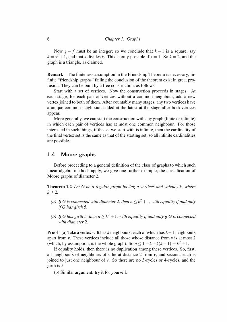
(b) There is a unique Moore graph with valency 3, the famous Petersen graph,shown below.
�������ZZ
ZZZZ��
����BBBBBBB���
SSS
���PPP
ZZ
ZZZ
�����
BBBBBB
������
t t
tt
tt t
t tt
Figure 1.3: The Petersen graph
This celebrated graph has been a counterexample to many plausible conjec-tures in graph theory, and has even had a book devoted entirely to it and its prop-erties (Derek Holton and John Sheehan, The Petersen Graph). We will say moreabout it in the next lecture.
It can be shown directly that there is no Moore graph of valency 4. (An outlineof a proof is given in the second appendix below.) But we are going to prove thefollowing theorem:
Theorem 1.3 If there exists a Moore graph of valency k, then k = 2, 3, 7, or 57.
There is a unique Moore graph of valency 7, the Hoffman–Singleton graph.I outline a construction of it in the appendix to this chapter. The existence ofa Moore graph of valency 57 is unknown: this is one of the big open problemsof extremal graph theory. Such a graph would have 3250 vertices, too large forcomputation! Graham Higman showed that it cannot have a vertex-transitive au-tomorphism group.
8 Chapter 1. Graphs
Proof Suppose that G is a Moore graph of valency k, and let A be its adjacencymatrix. We have
AJ = kJ, A2 = kI +(J− I−A).
The first equation holds for any regular graph. The second asserts that the numberof paths of length 2 from u to w is k if u = w, 0 if u ∼ w (since there are notriangles), and 1 otherwise (since there are no quadrilaterals but the diameter is 2.
As before, the all-1 vector is an eigenvector of A with eigenvalue k. Note thatthe second equation now gives k2 = k +(n− 1− k), or n = k2 + 1.) Any othereigenvector x is orthogonal to the all-1 vector, and so satisfies Jx = 0, from whichwe obtain the equation θ 2 = k−1−θ for the eigenvalue θ , giving
θ =−1±
√4k−3
2.
If these two eigenvalues have multiplicities f and g, we have
f +g = k2,
f (−1+√
4k−3)/2+g(−1−√
4k−3)/2 = −k.
Multiplying the second equation by 2 and adding the first gives
( f −g)√
4k−3 = k2−2k.
Now if k = 2, we have f = g = 2: this corresponds to a solution, the 5-cycle.Suppose that k > 2. Then the right-hand side is non-zero, so 4k−3 must be a
perfect square, say 4k− 3 = (2s− 1)2, so that k = s2− s+ 1. Then our equationbecomes ( f −g)(2s−1) = (s2− s+1)(s2− s−1).
So 2s− 1 divides (s2− s + 1)(s2− s− 1). Multiplying the right-hand sideby 16, and using the fact that 2s ≡ 1 (mod 2s− 1), we see that 2s− 1 divides(1− 2+ 4)(1− 2− 4) = −15, so that 2s− 1 = 1, 3, 5, or 15. This gives s = 1,s = 2, s = 3 or s = 8, and so k = 1, 3, 7 or 57. The case k = 1 gives a graph whichis a single edge, and doesn’t satisfy our condition of having diameter 2, so we areleft with the other three values.
1.5 Polarities of projective planes
The Friendship Theorem has a close link to finite geometry, which has beenrecognised from the time it was proved.
A projective plane is an incidence structure of points and lines satisfying theconditions
• any two points are incident with a unique line, and any two lines with aunique point;
• (nondegeneracy) there exist four points, no three collinear.

1.6. Appendix: symmetric matrices 9
Exercise Show that, if the nondegeneracy condition is weakened to the state-ment that no point lies on all lines, and no line contains all points, the only addi-tional structures that arise consist of a line L incident with all but one point P, and2-point lines joining P to the points of L.
The class of projective planes is self-dual; the nondegeneracy condition im-plies its dual. However, not every individual projective plane is “self-dual” (iso-morphic to its dual). We define a duality of a projective plane to be an isomor-phism from the plane to its dual (a pair of bijections from points to lines and fromlines to points which preserves incidence); it is a polarity if its square is the iden-tity. A point P is absolute (with respect to a polarity π) if it is incident with itsimage Pπ .
Theorem 1.4 Any polarity of a finite projective plane has absolute points.
Proof Suppose that π is a polarity with no absolute points. Form a graph whosevertices are the points of the plane, two vertices P and Q being adjacent if P isincident with Qπ (equivalently, Q is incident with Pπ ). Given any two points Pand Q, let L be the line incident with both, and let R = Lπ . Then R is the uniquecommon neighbour of P and Q.
By the Friendship Theorem, there is a point collinear with all others; that is,the projective plane is degenerate.
Remark As we noted after the proof of the Friendship Theorem, this is false forinfinite projective planes, which can be produced in great proliferation by a freeconstruction.
1.6 Appendix: symmetric matrices
Recall that a symmetric matrix A is a real matrix satisfying A = A>, while anorthogonal matrix P satisfies PP> = I. The following result is basic.
Theorem 1.5 Let A be a n×n real symmetric matrix. Then there is an orthogonalmatrix P such that P−1AP is diagonal. Equivalently, there is an orthonormal basisfor Rn consisting of eigenvectors of A.
This is the extension we need.
Theorem 1.6 Let A1,A2, . . . ,Am be n× n real symmetric matrices, and supposethat these matrices commute (that is, AiA j = A jAi for i, j = 1, . . . ,m). Then thereis an orthogonal matrix P such that P−1AiP is diagonal for i = 1, . . . ,m. Equiva-lently, there is an orthonormal basis for Rn consisting of simultaneous eigenvec-tors of A1, . . . ,Am.
10 Chapter 1. Graphs
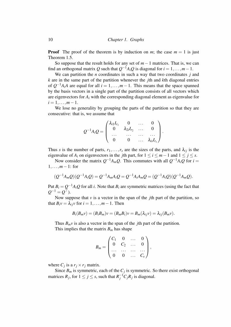
Proof The proof of the theorem is by induction on m; the case m = 1 is justTheorem 1.5.
So suppose that the result holds for any set of m−1 matrices. That is, we canfind an orthogonal matrix Q such that Q−1AiQ is diagonal for i = 1, . . . ,m−1.
We can partition the n coordinates in such a way that two coordinates j andk are in the same part of the partition whenever the jth and kth diagonal entriesof Q−1AiA are equal for all i = 1, . . . ,m− 1. This means that the space spannedby the basis vectors in a single part of the partition consists of all vectors whichare eigenvectors for Ai with the corresponding diagonal element as eigenvalue fori = 1, . . . ,m−1.
We lose no generality by grouping the parts of the partition so that they areconsecutive: that is, we assume that
Q−1AiQ =
λi1Ir1 0 . . . 0
0 λ2iIr2 . . . 0. . . . . . . . . . . .0 0 . . . λisIrs
.
Thus s is the number of parts, r1, . . . ,rs are the sizes of the parts, and λi j is theeigenvalue of Ai on eigenvectors in the jth part, for 1≤ i≤ m−1 and 1≤ j ≤ s.
Now consider the matrix Q−1AmQ. This commutes with all Q−1AiQ for i =1, . . . ,m−1: for
(Q−1AmQ)(Q−1AiQ) = Q−1AmAiQ = Q−1AiAmQ = (Q−1AiQ)(Q−1AmQ).
Put Bi = Q−1AiQ for all i. Note that Bi are symmetric matrices (using the fact thatQ−1 = Q>).
Now suppose that v is a vector in the span of the jth part of the partition, sothat Biv = λi jv for i = 1, . . . ,m−1. Then
Bi(Bmv) = (BiBm)v = (BmBi)v = Bm(λi jv) = λi j(Bmv).
Thus Bmv is also a vector in the span of the jth part of the partition.This implies that the matrix Bm has shape
Bm =
C1 0 . . . 00 C2 . . . 0. . . . . . . . . . . .0 0 . . . Cs
,
where C j is a r j× r j matrix.Since Bm is symmetric, each of the C j is symmetric. So there exist orthogonal
matrices R j, for 1≤ j ≤ s, such that R−1j C jR j is diagonal.
1.6. Appendix: symmetric matrices 11
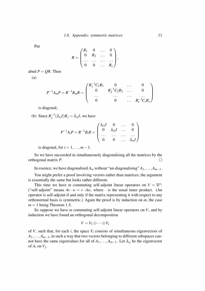
Put
R =
R1 0 . . . 00 R2 . . . 0. . . . . . . . . . . .0 0 . . . Rs
,
abnd P = QR. Then(a)
P−1AmP = R−1BmR =
R−1
1 C1R1 0 . . . 00 R−1
2 C2R2 . . . 0. . . . . . . . . . . .0 0 . . . R−1
s CsRs
is diagonal;
(b) Since R−1j (λi jI)R j = λi jI, we have
P−1AiP = R−1BiR =
λi1I 0 . . . 0
0 λi2I . . . 0. . . . . . . . . . . .0 0 . . . λisI
is diagonal, for i = 1, . . . ,m−1.
So we have succeeded in simultaneously diagonalising all the matrices by theorthogonal matrix P. �
In essence, we have diagonalised Am without “un-diagonalising” A1, . . . ,Am−1.
You might prefer a proof involving vectors rather than matrices; the argumentis essentially the same but looks rather different.
This time we have m commuting self-adjoint linear operators on V = Rn:(“self-adjoint” means Av ·w = v · Aw, where · is the usual inner product. (Anoperator is self-adjoint if and only if the matrix representing it with respect to anyorthonormal basis is symmetric.) Again the proof is by induction on m, the casem = 1 being Theorem 1.5.
So suppose we have m commuting self-adjoint linear operators on V , and byinduction we have found an orthogonal decomposition
V =V1⊕·· ·⊕Vs
of V , such that, for each i, the space Vi consists of simultaneous eigenvectors ofA1, . . . ,Am−1, in such a way that two vectors belonging to different subspaces can-not have the same eigenvalues for all of A1, . . . ,Am−1. Let λi j be the eigenvectorof Ai on Vj.

12 Chapter 1. Graphs
Since the Ai commute, if v ∈Vj, we have
Ai(Amv) = Am(Aiv) = Am(λi jv) = λi j(Amv).
Thus Amv is a simultanous eigenvector for A1, . . . ,Am−1, having the same eigen-values as v; thus Amv ∈Vj.
So Am maps Vj to itself. Clearly the restriction of Am to Vj is self-adjoint. Soby Theorem 1.5, there is an orthonormal basis for Vj consisting of eigenvectors ofAm. Clearly these vectors are still eigenvectors for A1, . . . ,Am−1.
Putting all these basis vectors together, and using the fact that Vj and Vk areorthogonal for j 6= k, we get an orthogonal matrix for the whole of V consistingof simultaneous eigenvectors of all of A1, . . . ,Am. �
A final note. If a set of symmetric matrices can be simultaneously diagonalisedby an orthogonal matrix, then they must commute. For suppose that P−1AiP = Diis diagonal for 1≤ i≤ m. Then Ai = PDiP−1, and so
AiA j = (PDiP−1)(PD jP−1) = PDiD jP−1 = PD jDiP−1 = A jAi,
since diagonal matrices commute.Now the two theorems stated above both remain true if we replace the real
numbers by the complex numbers, “symmetric” by “Hermitian”, and “orthogonal”by “unitary”. The proof is essentially the same: instead of transpose, simply useconjugate transpose.
But the converse is not true in this case; we need something a little moregeneral. A complex matrix A is said to be normal if it commutes with its conjugatetranspose: AA> = A>A. Now a normal matrix can be diagonalised by a unitarymatrix. In general, a set of complex matrices can be diagonalised by a unitarymatrix if and only if it consists of commuting normal matrices.
The proofs are left to you . . .
1.7 Appendix: Moore graphs
This appendix leads you through an elementary proof of the nonexistence of aMoore graph of diameter 2 and valency 4.
Recall that a Moore graph of diameter 2 and valency k is a connected graphwith diameter 2, girth 5, valency k, and having k2 + 1 vertices. Let G be such agraph. Let m = k−1.
(a) Let {u,v} be an edge. Show that the remaining vertices consist of three sets:
• A, the set of neighours of u other than v; the vertices of A are not joinedto one another or to v, and |A|= m.

1.7. Appendix: Moore graphs 13
• B, the set of neighours of v other than u; the vertices of B are not joinedto one another or to u, and |B|= m.• C, the set of vertices remaining: each vertex in C has one neighbour in
A and one in B, and each pair (a,b) with a ∈ A and b ∈ B correspondsto a unique vertex c ∈C in this manner, so that |C|= m2.
Check that 2+m+m+m2 = k2 +1. See the figure below.
(b) Identify C with A×B in the obvious way. Show that each vertex (a,b) of Chas m−1 neighbours in C, say (a1,b1), . . . ,(am−1,bm−1), where a,a1, . . . ,am−1are all distinct, as are b,b1, . . . ,bm−1.
(c) Suppose that m = 2, with A = {a1,a2} and B = {b1,b2}. Show that the onlypossibility for the edges in C is from (a1,b1) to (a2,b2) and from (a1,b2) to(a2,b1). Deduce the uniqueness of the Petersen graph.
(d) Suppose that m = 3, with A = {a1,a2,a3} and B = {b1,b2,b3}. Suppose,without loss of generality, that (a1,b1) is joined to (a2,b2) and (a3,b3).Show that necessarily (a2,b2) is joined to (a3,b3), in contradiction to thefact that there are no triangles. Deduce the non-existence of the Mooregraph with valency 4.
u u
�
�
�
�
�
�
�
�rrrrr
rrrrr
LLLLLLL
HHH
�������
���
����r##
##
##
cccccc
u v
A B
a b
C = A×B(a,b)
I mention briefly a construction of the Moore graph of valency 7: see Cameronand van Lint, Designs, Graphs, Codes and their Links, for further details. In thiscase, |A| = |B| = 6. We exploit the fact that the symmetric group of degree 6has an outer automorphism: that is, it has two different actions on sets of size6, which we can take to be A and B in our construction. These actions have theproperty that the element of S6 acting as a transposition (a1,a2) on A acts on B asthe product of three transpositions; if (b1,b2) is one of these three transpositions,then the element of S6 acting on B as the transposition (b1,b2) acts on A as theproduct of three transpositions, one of which is (a1,a2).
Now we complete the graph by putting an edge from (a1,b1) to (a2,b2) when-ever the above situation holds. Properties of the outer automorphism enable oneto show that this graph is indeed a Moore graph of valency 7.
CHAPTER 2
Strongly regular graphs
In the preceding section we met two examples of “strongly regular graphs”: pu-tative counterexamples to the Friendship Theorem, and Moore graphs. Now weexamine this class of graphs in more details.
2.1 Strongly regular graphs
A graph G is strongly regular with parameters (n,k,λ ,µ) if the followingconditions hold:
• G has n vertices;
• G is regular with valency k;
• the number of common neighbours of two distinct vertices v and w is λ ifv∼ w and µ otherwise.
The parameters are not all independent. Fix a vertex u, and count pairs (v,w)of vertices where u ∼ v ∼ w but u 6∼ w. If l denotes the number of vertices notjoined to u, we have
k(k−λ −1) = lµ,
so the parameters k,λ ,µ determine l, and hence n = 1+ k+ l. The argument alsogives us a divisibility condition: µ divides k(k−λ −1).
A regular counterexample to the Friendship Theorem would be a strongly reg-ular graph with λ = µ = 1, while a Moore graph of diameter 2 is a strongly regu-lar graph with λ = 0, µ = 1. So, for example, the Petersen graph has parameters(10,3,0,1).
14

2.1. Strongly regular graphs 15
Here are some strongly regular graphs.
• L(Km) is strongly regular with parameters (m(m−1)/2,2(m−2),m−2,4).(This graph is called the triangular graph T (m).)For clearly there are m(m−1)/2 vertices (edges of Km. Given an edge vw,it is adjacent to all edges vx and wx with x 6= v,w (so 2(m− 2) of these).Two adjacent edges uv and uw are joined to vw and to all ux with x 6= u,v,w:1+(m− 3) of these; and finally, nonadjacent edges uv and wz have fourcommon neighbours, uw, uz, vw and vz.Hoffman and Chang showed that, for m 6= 8, any strongly regular graph withthe same parameters as T (m) is isomorphic to T (m); for m = 8, there arethree exceptional graphs, the Chang graphs.. We will see the explanationfor this later.
• L(Km,m) is strongly regular with parameters (m2,2(m−1),m−2,2). (Thisgraph is called the square lattice graph L2(m). It can be viewed as m2
vertices in an m×m array, with vertices in the same row or column beingadjacent.)Shrikhande showed that, for m 6= 4, a strongly regular graph with the sameparameters as L2(m) is isomorphic to L2(m); for m = 4 there is a uniqueexception, the Shrikhande graph. Again we will see the reason later.
There are many more examples, derived from group-theoretic, geometric or com-binatorial configurations; we will meet some of them later in this course. Astrongly regular graph is a special case of a more general type of structure, anassociation scheme.
The disjoint union of complete graphs of size k+ 1 is strongly regular, withµ = 0. Such a graph is sometimes called “trivial”. Its complement is a completemultipartite graph, and is also strongly regular, with µ = k. (Indeed, the comple-ment of a strongly regular graph is again strongly regular – can you prove this?)
We now apply the eigenvalue methods we saw in the two examples. Theadjacency matrix A has an eigenvalue k with eigenvector the all-1 vector j, aswe see from the equation AJ = kJ. Any other eigenvector x can be taken to beorthogonal to j, and so satisfies Jx = 0; thus, if the eigenvalue is θ , we have
θ2x = A2x = ((k−µ)I +(λ −µ)A)x = ((k−µ)+λ −µ)θx,
and so θ 2− (λ −µ)θ − (k−µ) = 0.The roots of this equation give the other eigenvalues of A, which (by conven-
tion) are denoted r and s. Their product is −(k−µ), which is negative (if k 6= µ);so we assume that r > 0 and s < 0. We have
r,s = 12
(λ −µ±
√(λ −µ)2 +4(k−µ)
).

16 Chapter 2. Strongly regular graphs
If r and s have multiplicities f and g, then we have
f +g = n−1,f r+gs = −k,
the second equation coming from the fact that the trace of A is 0.These equations can be solved to give f and g, which must be non-negative
integers:
Theorem 2.1 If a strongly regular graph with parameters (n,k,λ ,µ) exists, thenthe numbers
f ,g = 12
(n−1± (n−1)(µ−λ )−2k√
(µ−λ )2 +4(k−µ)
)are non-negative integers.
To analyse further, we divide strongly regular graphs into two types:
Type I, with (n−1)(µ−λ ) = 2k. In this case
n = 1+2k
µ−λ> 1+ k,
so 0 < µ−λ < 2. So we must have µ−λ = 1, which gives λ = µ +1, k = 2µ ,n = 4µ +1. Examples of graphs of this type include the 5-cycle (with µ = 1) andL2(3) (with µ = 2).
Type 2, with (n−1)(µ−λ ) 6= 2k. In this case, we see that (µ−λ )2−4(k−µ)must be a perfect square, say u2; that u divides (n−1)(µ−λ )−2k, and that thequotient is congruent to n−1 (mod 2). This is the “general case”: most parametersets for strongly regular graphs fall into this case.
Example Consider the triangular graph, which has parameters(m(m−1)/2,2(m−2),m−2,4). We have√
(µ−λ )2 +4(k−µ) =√
(m−6)2 +8(m−4) = m−2,
and some further calculation gives the multiplicities of the eigenvalues as m− 1and m(m−3)/2, which are integers (as they should be).
2.2. Petersen, Clebsch and Schlafli graphs 17
Example Let us consider our previous examples.We saw that a counterexample to the Friendship Theorem would be strongly
regular, with λ = µ = 1 and n = k2− k+1. We find√(µ−λ )2 +4(k−µ) = 2
√k−1,
so k = s2 +1, where s divides k; we reach the same contradiction as before unlesss = 0.
A Moore graph of diameter 2 is strongly regular, with λ = 0, µ = 1, andn = k2 + 1. This time, Type 1 is possible, and corresponds to the 5-cycle. ForType 2, we have that 4k−3 is a perfect square, say (2u−1)2, where 2u−1 dividesk(k−2); again we reach the same conclusion as before.
2.1.1 Resources
Andries Brouwer keeps a list of parameter sets of strongly regular graphs on atmost 1300 vertices at http://www.win.tue.nl/~aeb/graphs/srg/srgtab.html
A list of strongly regular graphs on at most 64 vertices is maintained by TedSpence at http://www.maths.gla.ac.uk/~es/srgraphs.php (there may bemany different graphs with the same parameters – note that the list is not quitecomplete, see the documentation).
2.2 Petersen, Clebsch and Schlafli graphs
Three important graphs which play an important role in these lectures are thosenamed in the section title. They are strongly regular graphs having parametersrespectively (10,3,0,1), (16,5,0,2), and (27,10,1,5).
We already met the Petersen graph (and saw its portrait) in the last lecture.More formally, it is the complement of the line graph of K5: in other words, itsvertices can be labelled with the 2-element subsets of {1,2,3,4,5}, so that twovertices are joined if and only if their labels are disjoint.
Another construction of it is from the dodecahedral graph (the 1-skeleton ofthe dodecahedron). This graph has 20 vertices, falling into 10 “antipodal pairs”(lying at the maximum distance, namely 5, from each other). If we form a graphon 10 vertices by identifying antipodal vertices, we obtain the Petersen graph.
The Clebsch graph can be constructed as follows. Take a set A of size 5, say{1,2,3,4,5}. The vertices of the graph are the subsets of A of cardinality 1 or2, together with an extra vertex ∗. Edges are as follows (we identify a singletonsubset of A with an element of A):

18 Chapter 2. Strongly regular graphs
• ∗ is joined to the five elements of A;
• an element of A is joined to a 2-subset of A containing it;
• two 2-subsets of A are joined if and only if they are disjoint.
A relatively small amount of checking shows that this graph is regular with va-lency 5 and contains no triangles, while two vertices at distance 2 have two com-mon neighbours – in other words, it is strongly regular (16,5,0,2).
Another construction is from the 5-dimensional cube (the graph whose ver-tices are all 5-tuples of zeros and ones, two vertices joined if they agree in all butone coordinate, in other words, their Hamming distance is 1). For each vertex,there is a unique antipodal vertex at distance 5 (obtained by changing the 0s into1s and vice versa. Now, if we identify antipodal vertices, we obtain the Clebschgraph. This can be looked at another way. The set of 5-tuples containing an evennumber of ones (those with even Hamming weight) contains one vertex from eachantipodal pair, so we can regard these tuples as the vertices of the Clebsch graph;two vertices are joined if they differ in all but one position.
Note that the graph on the set of vertices not adjacent to a fixed vertex in theClebsch graph is the Petersen graph.
The Schlafli graph is defined in a somewhat similar way. The vertex setconsists of three parts: a set of ten vertices falling into five 2-sets {ai,bi} fori = 1, . . . ,5; the set of all 5-tuples of zeros and ones with even Hamming weight(an even number of ones); and one further vertex ∗. Edges are of three types:
• ∗ is joined to ai and bi for all i;
• a word w (a 5-tuple with even weight) is joined to ai if wi = 0, and to bi ifwi = 1;
• two words are joined if they differ in all positions except one.
Again, checking shows that the graph is strongly regular (27,10,1,5).The graph on the set of vertices not adjacent to a fixed vertex in the Schlafli
graph is the Clebsch graph.
Theorem 2.2 Each of the Petersen, Clebsch and Schlafli graphs is the uniquestrongly regular graph with its parameters (up to isomorphism).
Here is the proof of uniqueness of the Clebsch graph. The other two are leftas exercises for you.
Let G be a strongly regular graph with parameters (16,5,0,2). Let A be theset of five neighbours of a fixed vertex v, and B the set of non-neighbours. Theinduced subgraph on A is null, since λ = 0. Now µ = 2, from which we conclude
2.3. Partition into Petersen and Clebsch graphs 19
that any vertex in B has two neighbours in A, and any two vertices in A have aunique common neighbour in B. So vertices in B correspond to 2-element subsetsof A. Now a vertex in B has two neighbours in A, and so three in B. Two adjacentvertices in B must be indexed by disjoint subsets, since otherwise we would havea triangle. Since there are three pairs disjoint from a given one, the edges in Bare determined: two vertices are joined if and only if the pairs labelling them aredisjoint. So everything is determined.
2.3 Partition into Petersen and Clebsch graphs
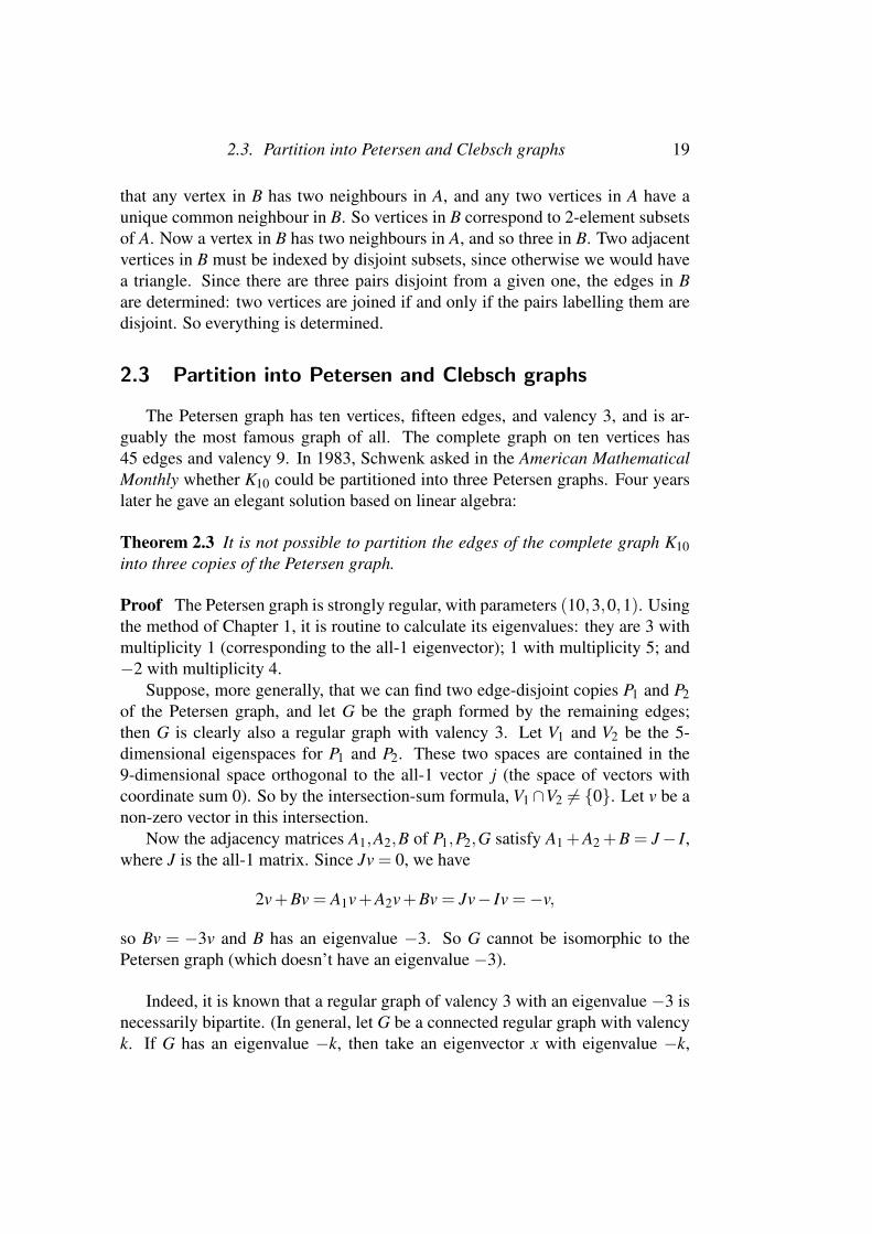
The Petersen graph has ten vertices, fifteen edges, and valency 3, and is ar-guably the most famous graph of all. The complete graph on ten vertices has45 edges and valency 9. In 1983, Schwenk asked in the American MathematicalMonthly whether K10 could be partitioned into three Petersen graphs. Four yearslater he gave an elegant solution based on linear algebra:
Theorem 2.3 It is not possible to partition the edges of the complete graph K10into three copies of the Petersen graph.
Proof The Petersen graph is strongly regular, with parameters (10,3,0,1). Usingthe method of Chapter 1, it is routine to calculate its eigenvalues: they are 3 withmultiplicity 1 (corresponding to the all-1 eigenvector); 1 with multiplicity 5; and−2 with multiplicity 4.
Suppose, more generally, that we can find two edge-disjoint copies P1 and P2of the Petersen graph, and let G be the graph formed by the remaining edges;then G is clearly also a regular graph with valency 3. Let V1 and V2 be the 5-dimensional eigenspaces for P1 and P2. These two spaces are contained in the9-dimensional space orthogonal to the all-1 vector j (the space of vectors withcoordinate sum 0). So by the intersection-sum formula, V1∩V2 6= {0}. Let v be anon-zero vector in this intersection.
Now the adjacency matrices A1,A2,B of P1,P2,G satisfy A1 +A2 +B = J− I,where J is the all-1 matrix. Since Jv = 0, we have
2v+Bv = A1v+A2v+Bv = Jv− Iv =−v,
so Bv = −3v and B has an eigenvalue −3. So G cannot be isomorphic to thePetersen graph (which doesn’t have an eigenvalue −3).
Indeed, it is known that a regular graph of valency 3 with an eigenvalue −3 isnecessarily bipartite. (In general, let G be a connected regular graph with valencyk. If G has an eigenvalue −k, then take an eigenvector x with eigenvalue −k,

20 Chapter 2. Strongly regular graphs
and partition the vertices into those with positive and negative sign; show that anyedge goes between parts of this partition.)
The next question is: Can the edge set of K16 be partitioned into three copiesof the Clebsch graph?
This time the answer is “yes”, and this fact is significant in Ramsey theory, aswe will briefly discuss. The construction is due to Greenwood and Gleason.
Here is the construction. Let F be the field GF(16). The multiplicative groupof F is cyclic of order 15, and so has a subgroup A of order 5, which has threecosets, say A,B,C in the multiplicative group. Now define three graphs as follows:The vertex set is the set F ; two vertices x,y are joined in the first, second, thirdgraph respectively if y− x lies in A, B, C respectively. Each graph has valency 5,since |A|= |B|= |C|= 5, and the three graphs are isomorphic (multiplication byan element of order 3 in the multiplicative group permutes them cyclically).
It can be shown that each of the three graphs is isomorphic to the Clebschgraph. Using the uniqueness, it is enough to show that they are all strongly regularwith parameters (16,5,0,2). The first two parameters are clear.
Let a,b,c,d,e be the fifth roots of unity in GF(16). These five elements sumto zero: Any 5th root of unity ω except 1 itself satisfies
1+ω +ω2 +ω
4 +ω5 = 0.
We claim that no proper subset sums to 0. Choose a subset of cardinality i. Ifi = 1, we would have (say) a = 0, which is not so. If i = 2, we would have (say)a+b = 0, so b = a (as the characteristic is 2), which again is not so. If i≥ 3, thenthe complementary set would also sum to zero, which again is not so.
Now, if (x1, . . . ,xk) is a cycle in the graph with “connection set” A, then eachof x2−x1, x3−x2, . . . , x1−xk would be a fifth root of unity, and these roots wouldsum to 0. So the graph contains no triangles; and the only 4-cycles are those ofthe form (x,x+a,x+a+b,x+b) for a,b ∈ A. Thus indeed λ = 0 and µ = 2.
Now, unlike what happened with the Petersen graph, if we remove the edgesof two edge-disjoint Clebsch graphs from K16, what remains must be anotherClebsch graph:
Proposition 2.4 The complement of two edge-disjoint Clebsch graphs in K16 isisomorphic to the Clebsch graph.
Proof As in the Petersen proof, we let A1 and A2 be the adjacency matrices for thetwo Clebsch graphs, and B the matrix for what remains. So we have A1+A2+B=J− I.
This time we find that the Clebsch graph has eigenvalues 5 (multiplicity 1),1 (multiplicity 10), and −3 (multiplicity 5). So each of A1 and A2 has a 10-dimensional space of eigenvectors with eigenvalue 1, contained in the 15-dimensional
2.4. Ramsey’s Theorem 21
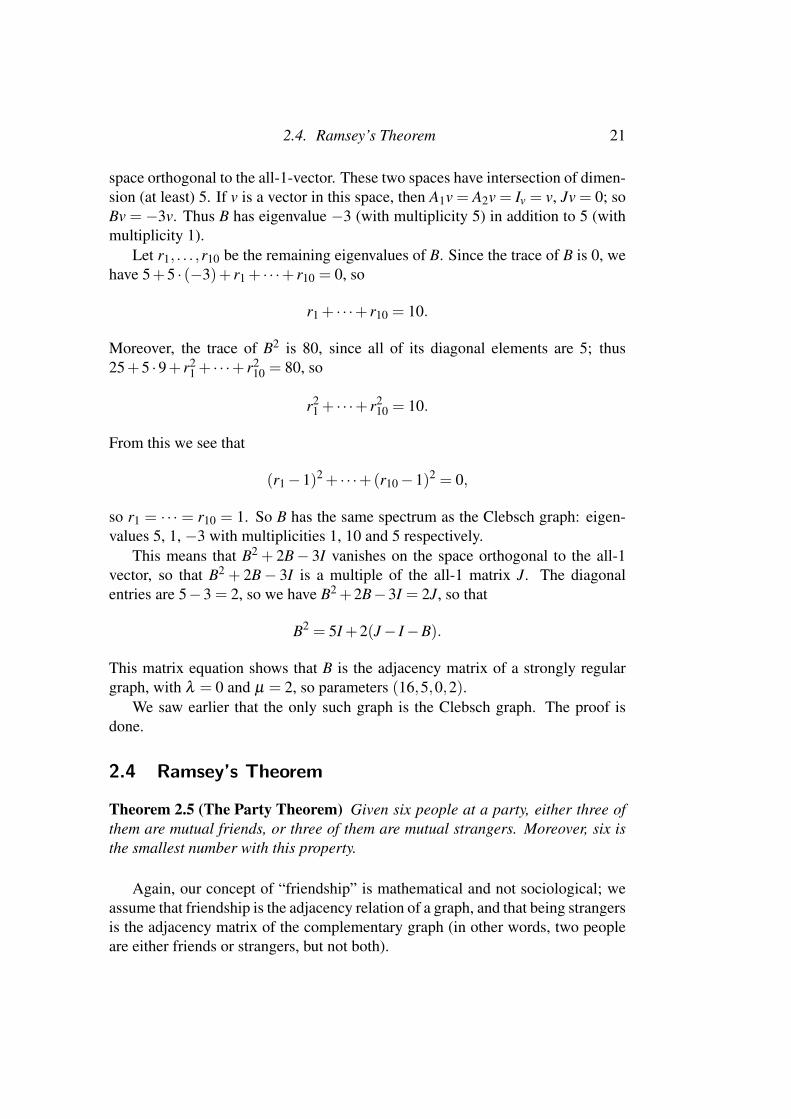
space orthogonal to the all-1-vector. These two spaces have intersection of dimen-sion (at least) 5. If v is a vector in this space, then A1v = A2v = Iv = v, Jv = 0; soBv = −3v. Thus B has eigenvalue −3 (with multiplicity 5) in addition to 5 (withmultiplicity 1).
Let r1, . . . ,r10 be the remaining eigenvalues of B. Since the trace of B is 0, wehave 5+5 · (−3)+ r1 + · · ·+ r10 = 0, so
r1 + · · ·+ r10 = 10.
Moreover, the trace of B2 is 80, since all of its diagonal elements are 5; thus25+5 ·9+ r2
1 + · · ·+ r210 = 80, so
r21 + · · ·+ r2
10 = 10.
From this we see that
(r1−1)2 + · · ·+(r10−1)2 = 0,
so r1 = · · · = r10 = 1. So B has the same spectrum as the Clebsch graph: eigen-values 5, 1, −3 with multiplicities 1, 10 and 5 respectively.
This means that B2 + 2B− 3I vanishes on the space orthogonal to the all-1vector, so that B2 + 2B− 3I is a multiple of the all-1 matrix J. The diagonalentries are 5−3 = 2, so we have B2 +2B−3I = 2J, so that
B2 = 5I +2(J− I−B).
This matrix equation shows that B is the adjacency matrix of a strongly regulargraph, with λ = 0 and µ = 2, so parameters (16,5,0,2).
We saw earlier that the only such graph is the Clebsch graph. The proof isdone.
2.4 Ramsey’s Theorem
Theorem 2.5 (The Party Theorem) Given six people at a party, either three ofthem are mutual friends, or three of them are mutual strangers. Moreover, six isthe smallest number with this property.
Again, our concept of “friendship” is mathematical and not sociological; weassume that friendship is the adjacency relation of a graph, and that being strangersis the adjacency matrix of the complementary graph (in other words, two peopleare either friends or strangers, but not both).

22 Chapter 2. Strongly regular graphs
Proof We have two things to do: to show that the assertion is true with six peoplebut false for five. In this case, the latter is easily dealt with: the pentagon or 5-cycle is a graph on 5 vertices containing no triangle; its complement is also a5-cycle and contains no triangle. (Think of the edges and diagonals of a 5-gon.)
Given six people at a party, select one of them, say A. Of the other five,according to the Pigeonhole Principle, either at least three are friends of A, orat least three are strangers to A. Let us consider the first case, and suppose thatB,C,D are friends of A. (The other case is similar.) If any two of B,C,D (say Band C) are friends, then we have three mutual friends A,B,C. If not, then B,C,Dare mutual strangers.
This theorem has a far-reaching generalisation, found in the 1930s. In order tostate it, we use the languge of colourings rather than friendship.
Theorem 2.6 (Ramsey’s Theorem) Let r,k, l1, . . . , lr be given positive integers.Then there exists a positive integer N such that, if the k-subsets of {1, . . . ,N} arecoloured with r colours, say c1, . . . ,cr, then there is some i with 1≤ i≤ r and a lisubset Li of {1, . . . ,N} so that every k-subset of Li has colour ci.
I will not prove the theorem here; the proof is just an elaboration of the argu-ment we saw for the Party Theorem. A consequence of Ramsey’s Theorem is thatthere is a smallest number N with the property of the theorem; we call this theRamsey number Rk(l1, . . . , lr).
Thus, the Party Theorem tells us that R2(3,3) = 6.Very few Ramsey numbers are known exactly (see the survey by Radzizowski
in the Electronic Journal of Combinatorics). For example, it is known that R2(4,4)=18, but R2(l, l) is not known for any larger value of l. In fact, Paul Erdos said that,if powerful aliens arrived and threatened to destroy the earth unless we told themthe value of R2(5,5), then we should put every mathematician and computer onthe planet to work on the problem; but if they asked for R2(6,6), our only hopewould be to get them before they got us.
One of the few values that is known is:
Theorem 2.7 R2(3,3,3) = 17.
Proof We suppose that the edges of K17 are coloured with three colours, say red,blue, green. Choose a vertex a. By the Pigeonhole Principle, there is a colour(let us say red) such that at least six vertices are joined to a by red edges – this isbecause 1+5+5+5 < 17. Let b,c,d,e, f ,g be vertices joined to a by red edges.If any of the edges within this set is red, we have a red triangle with a. If not, then{b, . . . ,g} is a set of six vertices with edges coloured blue and green; by the PartyTheorem, there is either a blue triangle or a green triangle within this set.

2.5. Regular two-graphs 23
Now we have to show that 16 is not enough. For that we use the configurationof three edge-disjoint Clebsch graphs. Colour their edges red, blue and greenrespectively; since each is a Clebsch graph, there is no triangle of a single colour.
2.5 Regular two-graphs
Regular two-graphs are objects introduced by Graham Higman to study var-ious doubly transitive permutation groups, especially the third Conway group.They have very close connections with strongly regular graphs, and also to otherstructures such as equiangular lines in Euclidean space (which are outside what Ican talk about here, unfortunately).
A regular two-graph (X ,T ) consists of a set X and a set T of 3-elementsubsets of X (which, to exclude degenerate cases, we assume is not the empty setand not the set of all 3-subsets of X) with the properties:
(a) any 4-element subset of X contains an even number of members of T ;
(b) any 2-element subset of X is contained in a constant number c of elementsof T (in other terminology, (X ,T ) is a 2-(|X |,3,c) design).
Given a regular two-graph (X ,T ), and a point x ∈ X , we define a graph Gx asfollows: the vertex set is X \{x}, and the vertices y and z are adjacent if and onlyif {x,y,z} ∈T .
Theorem 2.8 If (X ,T ) is a regular two-graph with parameter c, then for anyx ∈ X, the graph Gx defined above is a strongly regular graph (n−1,k,λ ,µ) withn = |X |, k = c, and µ = c/2.
Conversely, given a strongly regular graph G with µ = k/2, there is a regulartwo-graph (X ,T ), where X consists of the vertex set of X and a new isolatedvertex x, and T consists of the triples {y,z,w} containing an odd number an oddnumber of edges of G.
Proof We say that a 4-subset of X is complete if it contains four members ofT . Note that {x,y,z,w} is complete if and only if {y,z,w} is a triangle in Gx.(The forward implication is trivial; for the reverse, if {y,z,w} is a triangle, then{x,y,z,w} contains at least three members of T , and so is complete.
We show that any triple in T is contained in a constant number d of 4-sets,where |X | = 3c− 2d. Let {x,y,z} ∈ T . For any further point w, either all of{x,y,w}, {x,z,w} and {y,z,w} are in T (this happens for d points w) or exactlyone of them is (this happens c− d− 1 times for any given triple). So d + 3(c−d−1) = |X |−3 as required.
It now follows that Gx has valency k = c, and any two adjacent points haveλ = d common neighbours.
24 Chapter 2. Strongly regular graphs
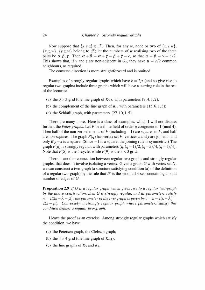
Now suppose that {x,y,z} /∈ T . Then, for any w, none or two of {x,y,w},{x,z,w}, {y,z,w} belong to T ; let the numbers of w realising two of the threepairs be α,β ,γ . Then α + β = α + γ = β + γ = c, so that α = β = γ = c/2.This shows that, if y and z are non-adjacent in Gx, they have µ = c/2 commonneighbours, as required.
The converse direction is more straightforward and is omitted.
Examples of strongly regular graphs which have k = 2µ (and so give rise toregular two-graphs) include three graphs which will have a starring role in the restof the lectures:
(a) the 3×3 grid (the line graph of K3,3, with parameters (9,4,1,2);
(b) the complement of the line graph of K6, with parameters (15,6,1,3);
(c) the Schlafli graph, with parameters (27,10,1,5).
There are many more. Here is a class of examples, which I will not discussfurther, the Paley graphs. Let F be a finite field of order q congruent to 1 (mod 4).Then half of the non-zero elements of F (including −1) are squares in F , and halfare non-squares. The graph P(q) has vertex set F ; vertices x and y are joined if andonly if y−x is a square. (Since−1 is a square, the joining rule is symmetric.) Thegraph P(q) is strongly regular, with parameters (q,(q−1)/2,(q−5)/4,(q−1)/4).Note that P(5) is the 5-cycle, while P(9) is the 3×3 grid.
There is another connection between regular two-graphs and strongly regulargraphs, that doesn’t involve isolating a vertex. Given a graph G with vertex set X ,we can construct a two-graph (a structure satisfying condition (a) of the definitionof a regular two-graph) by the rule that T is the set of all 3-sets containing an oddnumber of edges of G.
Proposition 2.9 If G is a regular graph which gives rise to a regular two-graphby the above construction, then G is strongly regular, and its parameters satisfyn = 2(2k−λ −µ); the parameter of the two-graph is given by c = n−2(k−λ ) =2(k− µ). Conversely, a strongly regular graph whose parameters satisfy thiscondition defines a regular two-graph.
I leave the proof as an exercise. Among strongly regular graphs which satisfythe condition, we have
(a) the Petersen graph, the Clebsch graph;
(b) the 4×4 grid (the line graph of K4,4);
(c) the line graphs of K5 and K8.

2.5. Regular two-graphs 25
To conclude this section, here is a design-theoretic construction of a very im-portant regular two-graph. This uses the famous 4-(23,7,1) Witt design, with 23points, 253 blocks, each block a set of seven points, and any four points containedin a unique block. It is known that there is a unique such design; it has the propertythat any two blocks intersect in 1 or 3 points.
Build a graph G, whose vertex set is P ∪B, where P and B are the pointand block sets of the design. Here are the edges:
• Any two vertices in P are adjacent.
• A vertex in P and a vertex in B are adjacent if and only if they are incident.
• Two vertices in B are adjacent if and only if their intersection has cardinal-ity 3.
Let X be the vertex set, and T the set of triples from X containing an odd numberof edges of G. Counting arguments show that this is a regular two-graph withparameter c = 162. (For example, if x,y ∈P , then there are 21 further points ofP (joined to both), 21 blocks containing both, and 120 blocks containing neither.)
The automorphism group of the two-graph is the third Conway group. (Thisconstruction was given by Graham Higman.)
The graph Gx we obtain from it is strongly regular with parameters (275,162,105,81).This is the McLaughlin graph.

CHAPTER 3
The Strong Triangle Property
We begin with one further result which looks superficially similar to the Friend-ship Theorem. However, this result, the classification of graphs with the StrongTriangle Property, will lead us on to root systems, graphs with smallest eigenvalue−2, characterisation of quadrics over the field of two elements, and more besides.
3.1 The Strong Triangle Property
We say that a graph G has the strong triangle property if
Every edge {u,v} of G is contained in a triangle {u,v,w} with theproperty that, for any vertex x /∈ {u,v,w}, x is joined to exactly one ofu,v,w.
Theorem 3.1 A graph with the strong triangle property is one of the following:
(a) a null graph;
(b) a Friendship Theorem graph (see Figure 1.1);
(c) one of three special graphs on 9, 15 and 27 vertices.
Remark The three special graphs are the line graph of K3,3, the complement ofthe line graph of K6, and the Schlafli graph; the three graphs we met in connectionwith regular two-graphs in the last section.
26

3.1. The Strong Triangle Property 27
Proof Let G be such a graph. If G has no edges, then (a) holds, so we mayassume there is at least one edge. Now we follow the proof of the FriendshipTheorem, by showing that either (b) holds or the graph is regular.
First we claim that, if u and v are not joined, then they have the same va-lency. For, given any vertex u, the subgraph on the closed neighbourhood of u is aFriendship Theorem graph, consisting of (say) m triangles joined at a vertex, andso u has valency 2m. Since v is not joined to u, it is joined to one vertex in eachof these triangles; so the neighbourhood of v consists of at least m triangles, and vhas valency at least 2m. Reversing the roles of u and v gives the claim.
Suppose that the graph is not regular, and let a and b be vertices with differentvalencies. There is a third vertex c joined to both, as in the Friendship Theorem.Now c has different valency from at least one of a and b, say a. Any further vertexis joined to exactly one of a,b,c, and also to at least one of a and b and at leastone of a and c; so it is joined to a, and we have a Friendship Theorem graph.
In the case when the graph is regular, we have that any two adjacent verticeshave one common neighbour, while two non-adjacent vertices have m commonneighbours, where 2m is the valency of the graph. So it is strongly regular, withparameters n,2m,1,m; and calculation shows that n = 6m− 3. (Note that, sincek = 2µ , the graph will give rise to a regular two-graph.)
Our analysis of strongly regular graphs in Chapter 2 shows that the eigenvaluesare 2m, 1 and −m. If their multiplicities are 1, f , g, we get
1+ f +g = 6m−3,2m+ f −mg = 0,
so (m+1)g = 8m−4. Thus m+1 divides 12, that is, m = 2, 3, 5 or 11.Further analysis shows that m = 11 is impossible while the graphs in the other
three cases are unique. (There is a bare-hands argument which comes up with thevalues 2, 3, 5 without using the strongly regular graph conditions; alternatively,the next result in the theory of strongly regular graphs beyond what we did in thelast lecture, the Krein condition, excludes the case m = 11.)
Here is the combinatorial argument. Let I be an index set for the set of trian-gles containing a given base point ∗; denote the two points of triangle i by (i,0)and (i,1). Now any point p not adjacent to ∗ is joined to one point in each triangle;so we can label p by a function wp : I→ {0,1}, where p is adjacent to (i,wp(i))for all i ∈ I. Now let p and q be non-neighbours of ∗, and consider the possiblerelations between p and q.
• If p and q are adjacent, then wp and wq agree in one point and differ inall others: for the third point in the triangle containing p an q has the form(i,ε) for some ε ∈ {0,1}, whence wp(i) = wq(i) = ε but there are no furtheragreements.

28 Chapter 3. The Strong Triangle Property
• If p and q are nonadjacent but have a common neighbour r not joined to ∗,then wp and wq agree in all but two positions; to see this, observe that allbut two values are changed twice as we go from p to r to q.
• Otherwise, every triangle on p contains a neighbour of ∗ and a neighbour rof q, and these two must be equal since there is a path prq which cannot liein the non-neighbourhood of ∗. So wp and wq agree everywhere: wp = wq.
But now, if |I| > 2, there is a path of length 3 in the set of non-neighbours of ∗,then all but three values of the function are changed three times, so the functionsassociated with the end points of the path agree in three points only. Since wecovered all cases, “three” must be equal to “all of I” or “all but two points of I”,and |I| ≤ 5, as required.
Note the finiteness of I is not assumed here. So there are no infinite regulargraphs with the strong triangle property, a fact we will meet again!
3.2 Root systems and the ADE affair
Root systems are geometric objects in Euclidean space, which crop up inmany parts of mathematics including Lie algebras, singularity theory, mathemati-cal physics, and graph theory.
In this section of the lectures, we will use graph theory to give the famous ADEclassification of root systems in which all roots have the same length. This willthen be used to determine the graphs whose adjacency matrix has least eigenvalue−2 or greater.
3.2.1 The definition
We work in the Euclidean space V = Rd , with the standard inner product.Given a non-zero vector u ∈ V , there is a unique hyperplane Hu through the
origin which is perpendicular to u. We define the reflection ru in this hyperplaneto be the linear map which fixes every vector in Hu and maps u to −u.
The formula for this reflection is
ru(x) = x− 2(x.u)u.u
u.
For this map is clearly linear, and does map u to −u and fixes every x satisfyingx.u = 0.
A root system is a set S of non-zero vectors of Rd satisfying the four conditions
• 〈S〉=V (S spans V );
• if u,λu ∈ S, then λ =±1;
3.2. Root systems and the ADE affair 29
• if u,v ∈ S, then 2(v.u)/(u.u) is an integer;
• for all u ∈ S, the reflection ru maps S to itself.
We remark that the first condition is not crucial, since we could replace V by thesubspace spanned by S to ensure that it holds. Also, the fourth condition impliesthe converse of the second (that is, if u ∈ S, then ru(u) =−u ∈ S). Also, the thirdcondition shows that ru(v) is an integer combination of u and v, for all u,v ∈ S.(This is called the crystallographic condition.)
Suppose that S1 and S2 are root systems in spaces V1 and V2. Then clearly S1∪S2 is a root system in the orthogonal direct sum of V1 and V2. Such a root systemis called decomposable; if there is no orthogonal direct sum decomposition with Sthe union of its intersections with the two summands it is called indecomposable.Clearly, to classify all root systems, it suffices to classify the indecomposableones, and take direct sums of them.
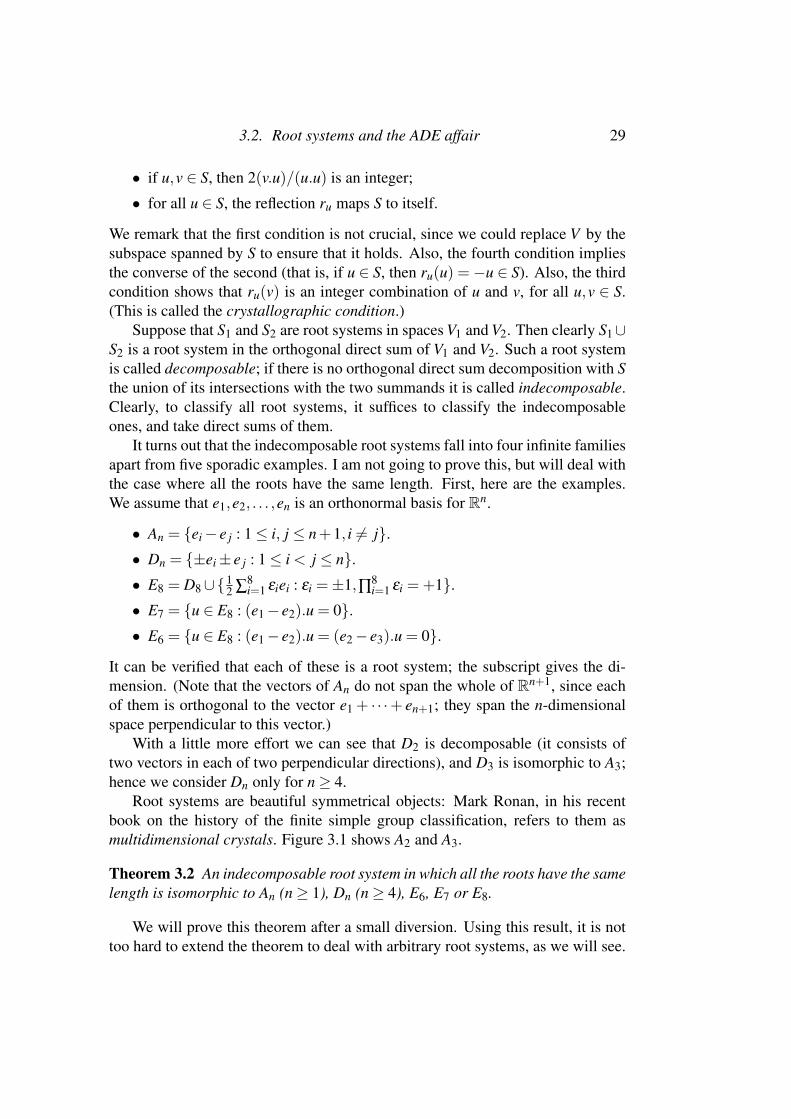
It turns out that the indecomposable root systems fall into four infinite familiesapart from five sporadic examples. I am not going to prove this, but will deal withthe case where all the roots have the same length. First, here are the examples.We assume that e1,e2, . . . ,en is an orthonormal basis for Rn.
• An = {ei− e j : 1≤ i, j ≤ n+1, i 6= j}.• Dn = {±ei± e j : 1≤ i < j ≤ n}.• E8 = D8∪{1
2 ∑8i=1 εiei : εi =±1,∏8
i=1 εi =+1}.• E7 = {u ∈ E8 : (e1− e2).u = 0}.• E6 = {u ∈ E8 : (e1− e2).u = (e2− e3).u = 0}.
It can be verified that each of these is a root system; the subscript gives the di-mension. (Note that the vectors of An do not span the whole of Rn+1, since eachof them is orthogonal to the vector e1 + · · ·+ en+1; they span the n-dimensionalspace perpendicular to this vector.)
With a little more effort we can see that D2 is decomposable (it consists oftwo vectors in each of two perpendicular directions), and D3 is isomorphic to A3;hence we consider Dn only for n≥ 4.
Root systems are beautiful symmetrical objects: Mark Ronan, in his recentbook on the history of the finite simple group classification, refers to them asmultidimensional crystals. Figure 3.1 shows A2 and A3.
Theorem 3.2 An indecomposable root system in which all the roots have the samelength is isomorphic to An (n≥ 1), Dn (n≥ 4), E6, E7 or E8.
We will prove this theorem after a small diversion. Using this result, it is nottoo hard to extend the theorem to deal with arbitrary root systems, as we will see.

30 Chapter 3. The Strong Triangle Property
r rr rr r
������
TTTTTT
��
��
��
��
��
��
��
��
r
r
�����������
r
r
�������
r
r
@@@
@@@@
rrAAAAr
r!!
!!!!
!!!
rr
QQQ
QQQ
Figure 3.1: The root systems A2 and A3
3.2.2 Proof of Theorem 3.2
Suppose we have an indecomposable root system in Rd with all roots of thesame length. Without loss of generality, we take this length to be
√2; so u.u = 2
for every root u, and u.v ∈ {2,1,0,−1,−2} for any roots u and v. This means thatany two roots are at an angle 0◦, 60◦, 90◦, 120◦ or 180◦. In other words, the linesspanned by the roots make angles 90◦ or 60◦ with each other.
There exist two roots u,v with u.v =−1 (in other words, an angle 120◦). Thenw =−u− v is also a root (it is −ru(v)). We call six roots of the form ±u, ±v and±w a star. (They form a root system of type A2 in the plane they span.)
Let S be a set of lines through the origin in Euclidean space Rd , any twomaking an angle 90◦ or 60◦. We say that S is star-closed if, whenever two linesL1,L2 ∈ S are at angle 60◦, the third line in their plane making an angle 60◦ withboth is also in S. (See Figure 3.2.)
.
................................................................................................................................................................................................................................................................................................................................................................................................................ .
................................................................................................................................................................................................................................................................................................................................................................................................................
Figure 3.2: A star
Proposition 3.3 Fix a positive number l. Then the vectors of length l in bothdirections along the lines of a set S form a root system if and only if the lines in Smake angles 90◦ or 60◦ with each other and the set S is star-closed.

3.3. Graphs with greatest eigenvalue ≤ 2 31
This is hopefully obvious from the preceding remarks. We will classify theroot systems by classifying the line systems with these properties instead.
If {〈u〉,〈v〉,〈w〉} is a star with u+v+w= 0, then any further root is orthogonalto one or all of u,v,w. For x.u,x.v,x.w ∈ {−1,0,1} and x.u+ x.v+ x.w = 0.
Let Au, Av, Aw, B be the sets of lines spanned by roots which are orthogonalto just u, just v, just w, or all three, and choose spanning roots on these lines sothat, for example, if 〈x〉 ∈ Au, then x.v =+1 and x.w =−1. Now form a graph Gwith vertex set Au, in which two vertices are adjacent if the corresponding linesare perpendicular.
First we claim that any two spanning vectors of lines in Au have non-negativeinner product. For if x,y are two such and x.y = −1, then 〈x+ y〉 ∈ Au, and (x+y).v = 2, which forces x+ y = v, a contradiction.
Next we claim that the graph G has the strong triangle property. For supposethat 〈x〉 and 〈y〉 are adjacent, so that x.y = 0. Then v− x and w+ y are roots, and(v− x).(w+ y) = 1; so v− x−w− y = z is a root. Checking inner products, wefind that 〈z〉 ∈ Ax. Now x+ y+ z = v−w, and so
(t.x)+(t.y)+(t.z) = 2
for all 〈t〉 ∈ Au. This means that exactly two of these three inner products are 1,so exactly one of the lines 〈x〉, 〈y〉 and 〈z〉 is perpendicular to 〈t〉 (and so joined toit in G).
Finally we claim that G determines the root system uniquely. For the graphstructure of G determines the inner products of vectors spanning the lines in
{〈u〉,〈v〉,〈w〉}∪Au;
and any other root can be obtained from these by closing under reflection.Now it is readily checked that, for the root systems An, Dn, E6, E7 and E8, the
structure of the graph G is null, a Friendship graph, or one of the three exceptionalgraphs in Theorem 3.1. This completes the proof.
For example, take the root system An, and let u = e1− e2, v = e2− e3 andw = e3− e1. Then Au consists of the lines spanned by vectors e2− ei for i > 3,and no two of these are orthogonal, so G is the null graph.
3.3 Graphs with greatest eigenvalue ≤ 2
The most iconic representation of the ADE root systems is given by the fa-mous “Coxeter–Dynkin diagrams”. Indeed, Francis Buekenhout suggested thatthey could be used in attempts to contact extraterrestrial civilisations, since anycivilisation advanced enough to receive our transmissions has almost certainlymet these ubiquitous diagrams!

32 Chapter 3. The Strong Triangle Property
E8 t t t t t t tt
E7 t t t t t tt
E6 t t t t tt
Dn(n≥ 4) t t t t ttt���
HHH . . . (n nodes)
An(n≥ 1)t t t t t t. . . (n nodes)
Figure 3.3: The ADE diagrams
Associated with each diagram is an “extended” diagram with one extra node:An is an (n+ 1)-cycle; Dn forks at both ends (if n = 4 it is a “star” with fourarms); and E6, E7 and E8 have arms where the numbers of edges are (2,2,2),(1,3,3) and (1,2,5) respectively. (Add one to each of these numbers: the resultsshould remind you of plane symmetry groups!)
I will not describe in detail how these are connected with the root systems.Here is their characterisation in graph-theoretic terms:
Theorem 3.4 (a) A connected graph whose adjacency matrix has greatest eigen-value less than 2 is a Coxeter–Dynkin diagram of type ADE, and conversely.
(b) A connected graph whose adjacency matrix has greatest eigenvalue 2 is anextended Coxeter–Dynkin diagram of type ADE, and conversely.
Proof First a general observation. By the Perron–Frobenius Theorem, if G is aconnected graph, then the largest eigenvalue of its adjacency matrix is a simpleeigenvalue with an eigenvector having every entry positive; if the graph is regular,then the largest eigenvalue is the degree. Moreover, the only eigenvectors withevery entry positive are multiples of this one.
Now show that each exteneded Dynkin diagram has largest eigenvalue 2. Thisis simply a case of writing down an eigenvector, that is, putting a number on eachvertex such that the sum of the numbers on neighbours of v is twice the numberon v. For An, this is easy: put 1 on each vertex. The eigenvector for E8 is shown.
Thus, a graph with largest eigenvalue strictly less than 2 cannot contain anyextended Dynkin diagram. In particular,

3.4. Graphs with least eigenvalue ≥−2 33
s s s s s s s ss
2 4 6 5 4 3 2 1
3
Figure 3.4: An eigenvector for E8
• it contains no cycle, so it is a tree;
• it has no vertex of valency 4, and at most one of valency 3;
• there are restrictions on the lengths of the arms if there is a vertex of valency3.
Only the Coxeter–Dynkin diagrams survive these conditions. This proves (a) oneway round; the converse holds since these graphs are contained in the extendeddiagrams, which have greatest eigenvalue 2, as we saw. The proof of (b) is similar,just a little more elaborate.
The usual proof of the characterisation of ADE root systems by Cartan andKilling works by showing that such a system has a “fundamental basis”, any twoof whose vectors have non-positive inner product; such a basis is represented by agraph with greatest eigenvalue less than 2, and the argument above determines it.
3.4 Graphs with least eigenvalue ≥−2
In this section, we use the classification of the root systems with all roots ofthe same length to determine the graphs G whose adjacency matrix A(G) has leasteigenvalue A(G) or larger.
Note that, if G is a graph with at least one edge, then the sum of the eigenvaluesof A(G) is zero (the trace of A(G), and hence G has both positive and negativeeigenvalues. So, for non-null graphs, the smallest eigenvalue is negative.
3.4.1 Preliminaries
Theorem 3.5 Let A= (ai j) be a positive semidefinite real symmetric n×n matrix.Then there are vectors v1, . . . ,vn ∈ Rd with vi.v j = ai j for all i and j, where d isthe rank of A.
Proof From the theory of real quadratic forms we know that, if A is a real sym-

34 Chapter 3. The Strong Triangle Property
metric matrix, then there exists an invertible matrix P such that
PAP> =
Ir O OO −Is OO O O
,
where r+s and r−s are the rank and signature of A. Since our matrix A is positivesemidefinite, we have s = 0, and so
PAP> =
(Id OO O
).
Put Q = P−1. Then
A = Q(
Id OO O
)Q> = Q1Q>1 ,
where Q1 is the matrix consisting of the first d columns of Q. Now if vi denotesthe ith row of Q1, the (i, j) entry of A = Q1Q>1 is equal to vi.v j, as required.
Here is an application, to point us in the direction we will go.
Proposition 3.6 Let G be a connected graph with smallest eigenvalue −1 (orgreater). Then G is a complete graph.
Proof Let A(G) be the adjacency matrix of G. By assumption, A(G)+ I is posi-tive semi-definite, so there are vectors v1, . . . ,vn with vi.v j equal to the (i, j) entry.Thus we have
• vi.vi = 1, so vi is a unit vector.
• if the ith and jth vertices are adjacent, then vi.v j = 1. But then(vi− v j).(vi− v j) = 0, and so vi = v j.
Since the graph is connected, all the vectors vi are equal. So vi.v j = 1 for all pairs(i, j); this means that G is a complete graph.
Indeed, the complete graph Kn has eigenvalues n−1 (with multiplicity 1) and−1 (with multiplicity n−1).
3.4.2 Generalised line graphs
In this section we define generalised line graphs. The definition is due to AlanHoffman, who proved the first version of the theorem given in the next section.
Our strategy is to represent a graph (if possible) by a set of vectors in Euclideanspace, where vi.vi = 2 for all i, and
vi.v j ={1 if vertices i and j are joined,
0 otherwise.
3.4. Graphs with least eigenvalue ≥−2 35
Proposition 3.7 A graph has a Euclidean representation in the above sense if andonly if its adjacency matrix has least eigenvalue −2 or greater.
Proof Suppse the least eigenvalue of A(G) has least eigenvalue −2 or greater.Then 2I +A(G) is positive semidefinite, and so represents the inner product of aset of vectors forming the required Euclidean representation. The other directionworks in the same way.
So which graphs can be represented?First we observe that any line graph has such a representation. Let G be a
graph on n vertices 1,2, . . . ,n. Take e1,e2, . . . ,en to be an orthonormal basis forRn. Then, for each edge i j in the graph G, we take the vector ei+e j. It is clear thateach vector has inner product 2 with itself, 1 with the vector ei + ek representingan edge sharing a vertex with i j, and 0 otherwise; so our conditions are satisfied.
Note that the representing vectors all lie in the root system Dn.Hoffman observed another class of graphs which are representable. The cock-
tail party graph CP(n) has 2n vertices, numbered 1,2, . . . ,2n; every pair of ver-tices is joined by an edge except for the pairs (2i−1),2i for i = 1,2, . . . ,n. (Thename reflects a cocktail party attended by n couples, each person talks to everyoneat the party except for his/her partner.)
The cocktail party graph can be represented in Rn+1, with standard basise0,e1, . . . ,en, in the following way: 2i− 1 7→ e0 + ei, 2i 7→ e0− ei. Again wehave a representation in a root system, this time Dn+1.
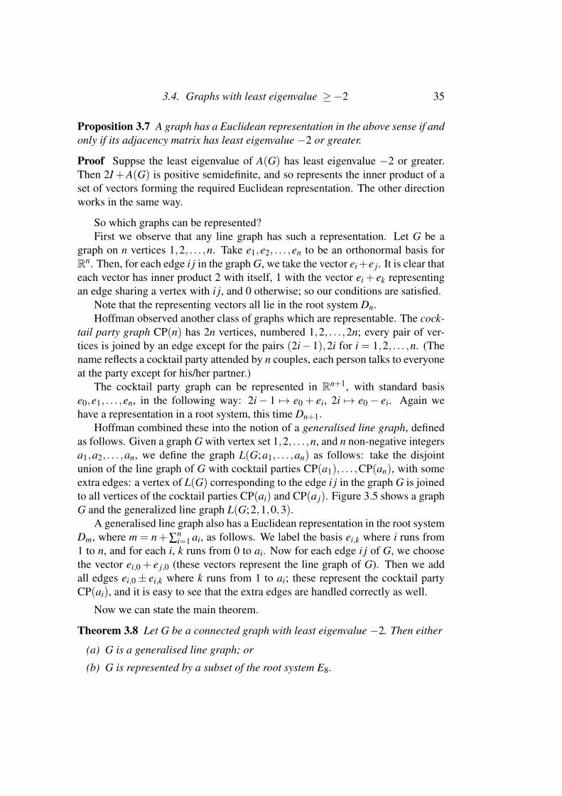
Hoffman combined these into the notion of a generalised line graph, definedas follows. Given a graph G with vertex set 1,2, . . . ,n, and n non-negative integersa1,a2, . . . ,an, we define the graph L(G;a1, . . . ,an) as follows: take the disjointunion of the line graph of G with cocktail parties CP(a1), . . . ,CP(an), with someextra edges: a vertex of L(G) corresponding to the edge i j in the graph G is joinedto all vertices of the cocktail parties CP(ai) and CP(a j). Figure 3.5 shows a graphG and the generalized line graph L(G;2,1,0,3).
A generalised line graph also has a Euclidean representation in the root systemDm, where m = n+∑
ni=1 ai, as follows. We label the basis ei,k where i runs from
1 to n, and for each i, k runs from 0 to ai. Now for each edge i j of G, we choosethe vector ei,0 + e j,0 (these vectors represent the line graph of G). Then we addall edges ei,0± ei,k where k runs from 1 to ai; these represent the cocktail partyCP(ai), and it is easy to see that the extra edges are handled correctly as well.
Now we can state the main theorem.
Theorem 3.8 Let G be a connected graph with least eigenvalue −2. Then either
(a) G is a generalised line graph; or
(b) G is represented by a subset of the root system E8.

36 Chapter 3. The Strong Triangle Property
r
rr r
���
���
@@@
@@@
1
2
3
4
r r
r rr
������
@@
@@
@@
23 34
12 14
13
rr rr��@@����CP(2)
��
@@
rr����CP(1)
���
@@@
rr rr rr����\\\\��
��XX
XX���ZZZ
����
��
@@
CP(3)
GL(G;2,1,0,3)
Figure 3.5: A generalised line graph
Remark In Hoffman’s earlier version of the theorem, condition (b) simply saidthat the number of vertices of G is bounded above by a constant. In fact, it can beshown easily that a graph represented by a subset of E8 has at most 36 vertices,and has valency at most 28; these bounds are best possible.
The proof depends on the following lemma.
Lemma 3.9 Let S be a set of vectors in Euclidean space such that
(a) v.v = 2 for all v ∈ S;
(b) v.w ∈ {−1,0,1} for all v,w ∈ S with w 6=±v.
Then S is a subset of a root system.
Proof We can adjoin to S the negatives of its vectors. Now suppose that v,w ∈ Swith v.w =−1. If v+w /∈ S, we consider inner products:
• (v+w).(v+w) = 2−2+2 = 2.
• Take any vector x ∈ S. Then x.(v+w) = x.v+ x.w, and each of x.v and
x.w is in {−1,0,1}. If x.v = x.w = 1, then x.(v+w) = 2, and so
(x− v−w).(x− v−w) = 2−2−2+2 = 0,
so x = v+w, contrary to the assumption that v+w /∈ S. A similar argu-ment holds if x.v = x.w = −1. We conclude that we can add v+w (and itsnegative) to S while preserving the hypotheses.
When this process terminates, we have a root system.

3.4. Graphs with least eigenvalue ≥−2 37
Proof of Theorem 3.8 To prove the theorem, take a graph with least eigenvalue−2 or greater. We know that it has a Euclidean representation, by a subset of aroot system, and so we only need to examine the root systems. Moreover, since Anis contained in Dn+1, we can assume that the root system is Dn (for some n) or E8;so to complete the proof, we only need to examine the case where the embeddingis into Dn.
So suppose G is a connected graph with a Euclidean representation as a subsetof Dn. We know that the vectors in the representation have non-negative innerproducts with each other. In particular, a vector and its negative cannot both occur.
Suppose that both ei+e j and ei−e j occur in the representation. Then no othervector can involve e j, and none can involve −ei. Thus we obtain a cocktail partygraph consisting of vectors ei± ek for some values of k. We call the vector ei theindex of this cocktail party.
If we have −ei + e j and −ei− e j, then we can change the sign of ei to obtaina cocktail party of the previous form with index ei.
Any other basis vector el occurs in only one of ±el± em, and we may assumethat it occurs with positive sign.
Then the vectors consist of a number of cocktail parties, and some vectorsei + el where each of ei and el is either the index of a cocktail party of one of theadditional vectors (which could be regarded as indices of empty cocktail parties).So we have reconstructed the graph, and it is a generalised line graph. (In detail,take the vertices of the graph G to be the indices of the cocktail parties, includingtrivial indices of empty cocktail parties; edges of G have the form il, where vi+vlis a vector in our set. Now we have precisely the representing set of the generalisedline graph L(G;a1, . . .), where CP(ai) is the cocktail party whose index is the ithvertex of G.)
Many characterisations of graphs by their eigenvalues can be deduced fromthis theorem. Here is an example, a theorem of Hoffman and Ray-Chaudhuri.(Originally, the theorem originally said “A sufficiently large connected regulargraph . . . is a line graph or a cocktail party graph”.)
Theorem 3.10 A connected regular graph whose ajacency matrix has least eigen-value −2 or greater is a line graph, a cocktail party graph, or is represented by asubset of E8.
Proof All we need to do is to show that a generalised line graph cannot be regularunless it is either a line graph or a cocktail party graph. So consider a generalisedline graph L(G;a1, . . . ,an), which has an edge i j and has ai > 0. Let di and d j bethe valencies of i and j in G. Then the vertex corresponding to the edge i j hasvalency (di− 1)+ (d j− 1)+ 2ai + 2a j, whereas a vertex in CP(ai) has valency

38 Chapter 3. The Strong Triangle Property
(2ai−2)+di. These differ by d j +2a j, where d j ≥ 1, a contradiction. So eitherG has one vertex and no edges (and we have just a cocktail party graph), or ai = 0for all i (and we have a line graph). The regular graphs represented by subsets ofE8 have been classified by Bussemaker, Cvetkovic and Seidel. There are 187 suchgraphs which are not line graphs or cocktail party graphs.
Another example is an even earlier theorem of Seidel (which, however, in-cluded a classification of all the exceptional graphs: there are exactly seven ofthem, the smallest being the Petersen graph). Seidel’s theorem extended earlierresults by Hoffman, Chang and Shrikhande. Indeed, the Shrikhande and Changgraphs we met earlier are represented in the root system E8, as well as the otherexceptions (the Petersen, Clebsch and Schlafli graphs).
Theorem 3.11 A strongly regular graph whose adjacency matrix has least eigen-value −2 is isomorphic to L(Km), L(Km,m), or CP(m), or is one of finitely manyexceptions.
The theorem in this form now follows if we can show that the only stronglyregular line graphs are L(Km), L(Km,m), and L(C5)∼=C5; this is an exercise.
3.5 The other root systems
In addition to the root systems of types An, Dn, E6, E7 and E8, there are furtherindecomposable root systems where roots can have different lengths.
Note that, if u and v are roots, with v 6=±u, then 2(u.v)/(u.u) and 2(u.v)/(v.v)are integers; their product is 4(u.v)2/(u.u)(v.v), which is strictly less than 4, bythe Cauchy–Schwarz inequality. So this product is 0, 1, 2 or 3. This means that,assuming v is longer than u, we have |v|=
√2|u| or |v|=
√3|u|. In particular, we
see that only two different lengths can occur, and they are in the ratio√
2 or√
3.Now in such a mixed root system, the roots of fixed length form a root system
(since reflections map them to themselves); this root system must be an orthogonaldirect sum of root systems of type ADE. A little more thought shows that thepossibilities are:
• two copies of A2, length ratio√
3 (this gives type G2);
• a copy of Dn together with an orthonormal basis, length ratio√
2 or 1/√
2(this gives types Bn and Cn);
• two copies of D4, length ratio√
2 (this gives type F4).
Thus we have the complete classification. B2 and G2 are shown below.The root system F4 can be represented (in terms of an orthonormal basis
e1,e2,e3,e4) by the vectors

3.5. The other root systems 39
���������@
@@@@@@@@
.
........................................................................................................................................................................................................ .
.........................................................................................................................................................................................................
..........................................................................................................................................................................................................................................................................................................................................................
.
............................................................
............................................................
............................................................
............................................................
............................................................
..............................................
Figure 3.6: The root systems B2 and G2
• ±e1, ±e2, ±e3, ±e4 (8 vectors);
• ±ei± e j (i 6= j) (24 vectors);
• (±e1± e2± e3± e4)/2 (16 vectors).
These root systems also have applications to spectral graph theory. A theoremof Whitney asserts that graphs G and G′ on more than four vertices which haveisomorphic line graphs must themselves be isomorphic. (An exception on fourvertices is given by the two graphs in Figure 3.7.
u uuu
�����
TTTTT
u uuu
"""
bbb
Figure 3.7: Graphs with isomorphic line graphs
This theorem can be extended to generalised line graphs. If L(G;a1, . . . ,an)and L(H;b1, . . . ,bm) are isomorphic, and n+∑ai > 4, then G is isomorphic to H,so m = n, and ai = bi for i = 1, . . . ,n.
This is proved by representing the edge set of a generalised line graph by asubset of a root system of type Dn as before. Now vertices correspond to unit vec-tors having inner product 0 or ±1 with all the vectors of Dn. If n > 4, then addingin these vectors gives a root system of type Bn, and the vertices are uniquely de-fined. The exceptional cases correspond to the exceptional root system F4.
Exercise In R4, with orthonormal basis {e1,e2,e3,e4}, the vectors ei + e j, for1 ≤ i < j ≤ 4, represent L(K4). Find another orthonormal basis f1, f2, f3, f4 rel-ative to which these vectors have the form f1± fk f or k = 2,3,4 (representingCP(3) = L(K1;3)).

CHAPTER 4
Polar spaces
4.1 Vector spaces over GF(2)
Vector spaces over the field of two elements are particularly easy to recogniseand pleasant to work in. If X denotes a basis for such a vector space, then anarbitrary vector v has coordinates 0 and 1 relative to X , and so defines a subset ofX , the set of basis vectors which occur with coefficient equal to 1. The correspon-dence between the vector space and the power set of X is a bijection; addition ofvectors corresponds to symmetric difference of subsets.
The projective space based on such a vector space is also easy to recognise.In general, the points and lines of the projective space based on a vector space Vcorrespond to the 1-dimensional and 2-dimensional subspaces of V . Over GF(2),a 1-dimensional space has the form {0,v} for some non-zero vector v, so pointscan be identified with elements of V \ {0}; any 2-dimensional subspace has theform {0,u,v,w}, where w= u+v, and so the lines can be identified with the triplesof points having sum 0.
The Veblen–Young characterisation of projective space is also very simple.
Theorem 4.1 An incidence structure of points and lines is a projective space overGF(2) if and only if it satisfies the following:
(a) any line contains exactly three points;
(b) two points lie on a unique line;
(c) if a line meets two sides of a triangle, not at a vertex, then it meets the thirdside also (see Figure 4.1).
40

4.1. Vector spaces over GF(2) 41
s s s
ss s������
BBBBBB
PPPP
PPPP
Figure 4.1: Veblen–Young axiom (c)
Proof To prove the theorem we have to reconstruct the vector space. The obviousway to do this is to define V = P∪ {0}, where P is the point set and 0 a newsymbol; then define addition by
v+0 = 0+ v = v, v+ v = 0, u+ v = w if {u,v,w} is a line,
and scalar multiplication by
0.v = 0 1.v = v,
and prove that this is a vector space over GF(2). The only thing that is not obviousis the associative law, which follows from condition (c).
However, I will give a different proof, which is a gentle introduction to theargument (of Jonathan Hall) we use later to recognise polar spaces over GF(2).
Let V be the vector space of functions from P to GF(2). This space has a basisconsisting of the characteristic functions x of singleton subsets {x} of P. Nowlet R be the subspace of V spanned by all vectors of the form u+ v+ w, where{u,v,w} is a line of the projective space, and V = V/R. Let x be the image of x inV . We are going to show that
• the map P→V given by x 7→ x is one-to-one, and its image is V \{0}, where0 is the zero of V ;
• u+ v+ w = 0 if and only if {u,v,w} is a line.
The result will follow.We show that, if S is a set of points with ∑{v : v ∈ S} = 0, then |S| ≥ 3, with
equality if and only if S is a line. This clearly establishes the second point above.Suppose that it holds. Then clearly x 6= 0 and x+ y 6= 0 for all distinct x,y, so thefirst point holds too.
If a set S has sum zero as above, and two points x,y belong to S, then eitherthe third point z on the line through xy belongs to S, or we can replace x and yby z to get a smaller set. So we may assume that |S| = 1, say S = {v}. Nowv = 0 means that there is a set L of lines such that the sum of the correspondingspanning vectors of R is v; that is, v lies on an odd number of lines of L and every

42 Chapter 4. Polar spaces
other point on an even number. Suppose that, subject to this, |L | is minimal.Then there is no triangle formed by lines of L (since we could replace {a,b,z},{a,c,y}, {b,c,x} by {x,y,z}, which is a line by the VY axiom).
The set L must contain a cycle. But any cycle can be shortened, which con-tradicts the fact that there are no triangles. For suppose that {a,b,c}, {c,d,e},{e, f ,g} and {g,h, i} are lines in L . Let {c,g, j} be the line on c and g. Then{d, f , j} is a line; replacing {c,d,e} and {e, f ,g} by {c,g, j} and {d, f , j} gives ashorter cycle, as claimed.
4.2 Quadratic and bilinear forms
Let V be a vector space over a field F . A bilinear form B on V is a functionfrom V ×V to F , which is linear in each variable (the other being fixed): that is,
B(v1 + v2,w) = B(v1,w)+B(v2,w), B(cv,w) = cB(v,w),B(v,w1 +w2) = B(v,w1)+B(v,w2), B(v,cw) = cB(v,w)
for all v, . . . ,∈V and c ∈ F .A bilinear form B has a left and a right radical, defined by
LB = {v ∈V : (∀w ∈V )B(v,w) = 0,RB = {w ∈V : (∀v ∈V )B(v,w) = 0.
If V is finite-dimensional, the radicals have the same dimension. We say that B isnon-degenerate if they are equal to {0}.
A bilinear form B is reflexive if B(v,w) = 0 if and only if B(w,v) = 0. Clearlythe left and right radicals of a reflexive form are equal.
Theorem 4.2 A non-degenerate reflexive bilinear form is either
• symmetric, that is, B(v,w) = B(w,v) for all v,w ∈V ; or
• alternating. that is, B(v,v) = 0 for all v ∈V .
Note that, if B is alternating, then expanding B(v+w,v+w) = 0 we find thatB(v,w) =−B(w,v). In particular,
• if the characteristic of F is not 2, then only the zero form is both symmetricand alternating;
• if the characteristic is 2, then an alternating form is symmetric.

4.2. Quadratic and bilinear forms 43
Non-degenerate alternating bilinear forms can be defined on V if and only if thedimension of V is even.
A quadratic form on a vector space V over F is a function Q : V →F satisfyingthe conditions
• Q(cv) = c2Q(v) for all c ∈ F , v ∈V ;
• the function B(v,w) = Q(v+w)−Q(v)−Q(w) is bilinear.
The bilinear form B is said to be obtained by polarisation of Q.The behaviour depends on the characteristic of F :
• If the characteristic of F is not 2, then B is a symmetric bilinear form, andQ can be recovered from B by Q(v) = 1
2B(v,v).
• If the characteristic of F is 2, then B is an alternating bilinear form, and Qis not recoverable from Q.
• In the special case where F has two elements, the set of quadratic formswhich polarise to a given alternating bilinear form is a coset of the spaceof linear forms on V (the dual space of V ), so there are 2n such quadraticforms, where n = dim(V ).
A quadratic form Q (which polarises to B) is said to be non-singular if Q(v) =0 and B(v,w) = 0 for all w ∈ V imply v = 0. If the characteristic is not 2, then Qis non-singular if and only if B is non-degenerate. However, if the characteristicis 2, then it may happen that B has 1-dimensional radical and Q is non-zero on thenonzero vectors of the radical. Indeed, in the case where |F | = 2, the restrictionof Q to the radical of B is a linear function, so its kernel has codimension 1; thus,for a non-singular form, the radical has dimension at most 1.
We conclude this brief survey with a result about defining forms by their valueson a basis.
Proposition 4.3 Let V be a vector space with basis {e1, . . . ,en}.
(a) We can define a bilinear form B on V by specifying the values B(ei,e j) for1≤ i, j ≤ n.
(b) In characteristic 2, if we specify B(ei,ei)= 0 for all i and B(ei,e j)=B(e j,ei)for all i, j, then B is alternating.
(c) In characteristic 2, given an alternating bilinear form B, we can define aquadratic form Q polarising to B by specifying the values Q(ei) for 1≤ i≤n.

44 Chapter 4. Polar spaces
Proof (a) Given B on a basis, we define
B
(∑
ixiei,∑
jy je j
)= ∑
i∑
jxiy jB(ei,e j).
(b) If B(ei,ei) = 0 for all i and the characteristic is 2, then
B
(∑
ixiei,∑
ixiei
)= 2 ∑
i< jxix jB(ei,e j) = 0
because of the factor 2.(c) Given the values of Q(ei), we have
Q(xiei + x je j) = x2i Q(ei)+ x2
yQ(e j)+ xix jB(ei,e j),
and similarly we extend Q to linear combinations of more than two basis vectors.
4.3 The Triangle Property
In this section, we give a generalisation of Theorem 3.1, the classification ofgraphs with the strong triangle property.
Theorem 4.4 Let G be a graph with the triangle property. Then one of the fol-lowing holds:
(a) G is a null graph;
(b) there is a vertex of Γ joined to all others;
(c) G is the graph associated with a non-singular formed space over GF(2).
The theorem is due to Shult, with a refinement by Seidel. The proof given hereis by Jonathan Hall: with small modifications it works for infinite graphs as wellas finite ones.
Proof The null graph clearly satisfies the hypotheses; so we may assume that Gis not null. We also assume that (b) does not hold, that is, there is no vertex joinedto all others.
It follows from this assumption that, given an edge {u,v}, the third vertex wspecified in the triangle property is unique. For suppose that the triangles {u,v,x}and {u,v,y} both satisfy the conditions of the triangle property. Then y is joinedto u and v, and so also with x; so there is a triangle {x,y,z} for some z, and both u

4.3. The Triangle Property 45
and v are joined to z. Any further point is joined to both or neither x and y, and sois joined to z, contradicting the assumption.
Let X be the vertex set of the graph G, and let F = GF(2). We begin with thevector space V of all functions from X to F , with pointwise operations. Let x ∈ Vbe the characteristic function of the singleton set {x}. The functions x, for x ∈ X ,form a basis for V . We define a bilinear form B on V by setting
B(x, y) ={
0 if x = y or x is joined to y,1 otherwise,
and extending linearly. Then we define a quadratic form Q by setting Q(x) = 0for all x ∈ X and extending to V by the rule
Q(v+w) = Q(v)+ Q(w)+ B(v,w).
Note that both B and Q are well-defined, by our remarks before the theorem.Let R be the radical of Q; that is, R is the subspace
{v ∈ V : Q(v) = 0, B(v,w) = 0 for all w ∈ V},
and set V = V/R. Then B and Q induce bilinear and quadratic forms B,Q on V : forexample, we have Q(v+R) = Q(v) (and this is well-defined, that is, independentof the choice of coset representative). Now let x = x+R ∈V .
We claim that the embedding x 7→ x has the required properties; in other words,it is one-to-one; its image is the set of singular points of Q; and two vertices x,y areadjacent if and only if the corresponding vectors x, y are orthogonal. We proceedin a series of steps.
Step 1 Let {x,y,z} be a special triangle, as in the statement of the triangle prop-erty. Then x+ y+ z = 0.
It is required to show that r = x+ y+ z ∈ R. We have
B(r, v) = B(x, v)+ B(y, v)+ B(z, v) = 0
for all v ∈ X , by the triangle property; and
Q(r) = Q(x)+ Q(y)+ Q(z)+ B(x, y)+ B(y, z)+ B(z, x) = 0
by definition.
Step 2 The map x 7→ x is one-to-one on X.Suppose that x = y. Then r = x+ y ∈ R. Hence B(x, y) = 0, and so x is joined
to y. Let z be the third vertex of the special triangle containing x and y. Thenz = x+ y ∈ R by Step 1, and so z is joined to all other points of X , contrary toassumption.
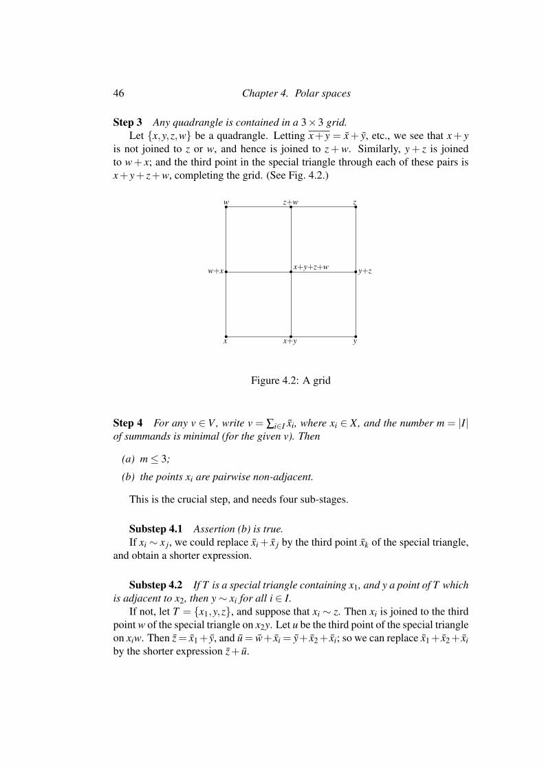
46 Chapter 4. Polar spaces
Step 3 Any quadrangle is contained in a 3×3 grid.Let {x,y,z,w} be a quadrangle. Letting x+ y = x+ y, etc., we see that x+ y
is not joined to z or w, and hence is joined to z+w. Similarly, y+ z is joinedto w+ x; and the third point in the special triangle through each of these pairs isx+ y+ z+w, completing the grid. (See Fig. 4.2.)
r r r
r r r
r r r
x x+y y
y+z
zz+ww
w+x x+y+z+w
Figure 4.2: A grid
Step 4 For any v ∈ V , write v = ∑i∈I xi, where xi ∈ X, and the number m = |I|of summands is minimal (for the given v). Then
(a) m≤ 3;
(b) the points xi are pairwise non-adjacent.
This is the crucial step, and needs four sub-stages.
Substep 4.1 Assertion (b) is true.If xi ∼ x j, we could replace xi + x j by the third point xk of the special triangle,
and obtain a shorter expression.
Substep 4.2 If T is a special triangle containing x1, and y a point of T whichis adjacent to x2, then y∼ xi for all i ∈ I.
If not, let T = {x1,y,z}, and suppose that xi ∼ z. Then xi is joined to the thirdpoint w of the special triangle on x2y. Let u be the third point of the special triangleon xiw. Then z= x1+ y, and u= w+ xi = y+ x2+ xi; so we can replace x1+ x2+ xiby the shorter expression z+ u.
4.4. The Buekenhout–Shult Theorem 47
Substep 4.3 There are two points y,z joined to all xi.Each special triangle on x1 contains a point with this property, by Substep 4.2.
It is easily seen that if x1 lies in a unique special triangle, then one of the pointson this line is adjacent to all others, contrary to assumption.
Substep 4.4 m≤ 3.Suppose not. Considering the quadrangles {x1,y,x2,z} and {x3,y,x4,z}, we
find (by Step 3) points a and b with
x1 + y+ x2 + z = a, x3 + y+ x4 + z = b.
But then x1 + x2 + x3 + x4 = a+ b, a shorter expression.
Step 5 If v ∈V , v 6= 0, and Q(v) = 0, then v = x for some x ∈ X.If not then, by Step 4, either v = x+ y, or v = x+ y+ z, where points x,y (and
z) are (pairwise) non-adjacent. In the second case,
Q(v) =Q(x)+Q(y)+Q(z)+B(x, y)+B(y, z)+B(z, x) = 0+0+0+1+1+1= 1.
The other case is similar but easier.
Step 6 x∼ y if and only if B(x, y) = 0.This is true by definition, since B(x, y) = B(x, y).
4.4 The Buekenhout–Shult Theorem
This section describes a wide generalisation of the material in the precedingsection. I will give only a general description, with no proofs. Also we willconsider only finite fields. (Additional complications arise in the infinite case!)
We met vector spaces carrying various kinds of forms (non-degenerate alter-nating bilinear forms, or non-singular quadratic forms). There is a third kind ofform to be considered in conjunction with these, non-degenerate Hermitian forms.Such a form is sesquilinear, that is, linear in the first variable and semilinar in thesecond (this means there is an associated field automorphism σ such that
B(v,w1 = w2) = B(v,w1)+B(v,w2), B(v,cw) = cσ B(v,w).
We pause to recall that the automorphism group of a finite field of order q = pr
(wherer p is prime) is cyclic of order n, generated by the Frobenius map x 7→ xp.A Hermitian form is a non-degenerate (that is, radical is zero) sesquilinear
form satisfying B(w,v) = B(v,w)σ , where σ is the associated field automorphism.It is immediate that σ2 = 1, so that q = q2
0 and σ is the map x 7→ xq0 .
48 Chapter 4. Polar spaces
Now alternating bilinear forms, quadratic forms, and Hermitian forms can betreated together. The geometry associated with such a form is called a polar space;its points, lines, . . . , are the points, lines, . . . of the projective space which aretotally isotropic (in the case of bilinear or Hermitian forms) or totally singular (forquadratic forms), that is to say, the form vanishes on the subspace. The maximumvector space dimension of such a subspace is called the Witt index of the space.If the Witt index is r, then the vector space dimension n of V is at least 2r, andis at most 2r+2 (in the case of a quadratic form), 2r+1 (for a Hermitian form),and 2r (for an alternating form). Thus there are six kinds of polar space. Thosecoming from a quadratic form are called quadrics, and are elliptic, parabolic orhyperbolic according as n = 2r+ 2, n = 2r+ 1, or n = 2r. (Remember that thegeometric dimension is n−1.)
Now with a polar space we associate a graph as follows: the vertices are thepoints of the polar space; two vertices are joined if and only if they are orthog-onal with respect to the sesquilinear form, that is, they are contained in a totallyisotropic or totally singular line.
The Buekenhout–Shult theorem gives a unified characterisation of all thesepolar spaces, in the finite case, in terms of this graph.
Theorem 4.5 Let G be a finite graph with the property that any edge of G iscontained in a clique (a complete subgraph) C with |C| > 2 such that any vertexoutside C is joined to one or all points of C. Then one of the following holds:
• G is a null graph;
• G has a vertex which is joined to all other vertices;
• G is the graph associated with a non-degenerate polar space.
(Note that the polar spaces here include generalised quadrangles, which wewill consider in the next section.)
Note how this theorem is a natural generalisation of the characterisation ofgraphs with the triangle property. Unlike that theorem, in this case the vectorspace is not constructed directly from the graph, but instead the entire polar spaceis reconstructed, and a theorem of Veldkamp and Tits is used to recognise it.
Note also that there is a version of the theorem not assuming finiteness. It isnecessary to assume finite rank (that is, chains of subspaces, suitably defined, arerequired to be finite), and also there are some other types of spaces which have tobe added to the list.
For an example of this, the lines in the 3-dimensional vector space over a fieldF carry the structure of a graph satisfying the hypothesis. (There are two types ofcliques: the set of lines in a plane, and the set of lines in the pencil through a point.The hypothesis is easily checked.) If F is commutative, then this is isomorphic to
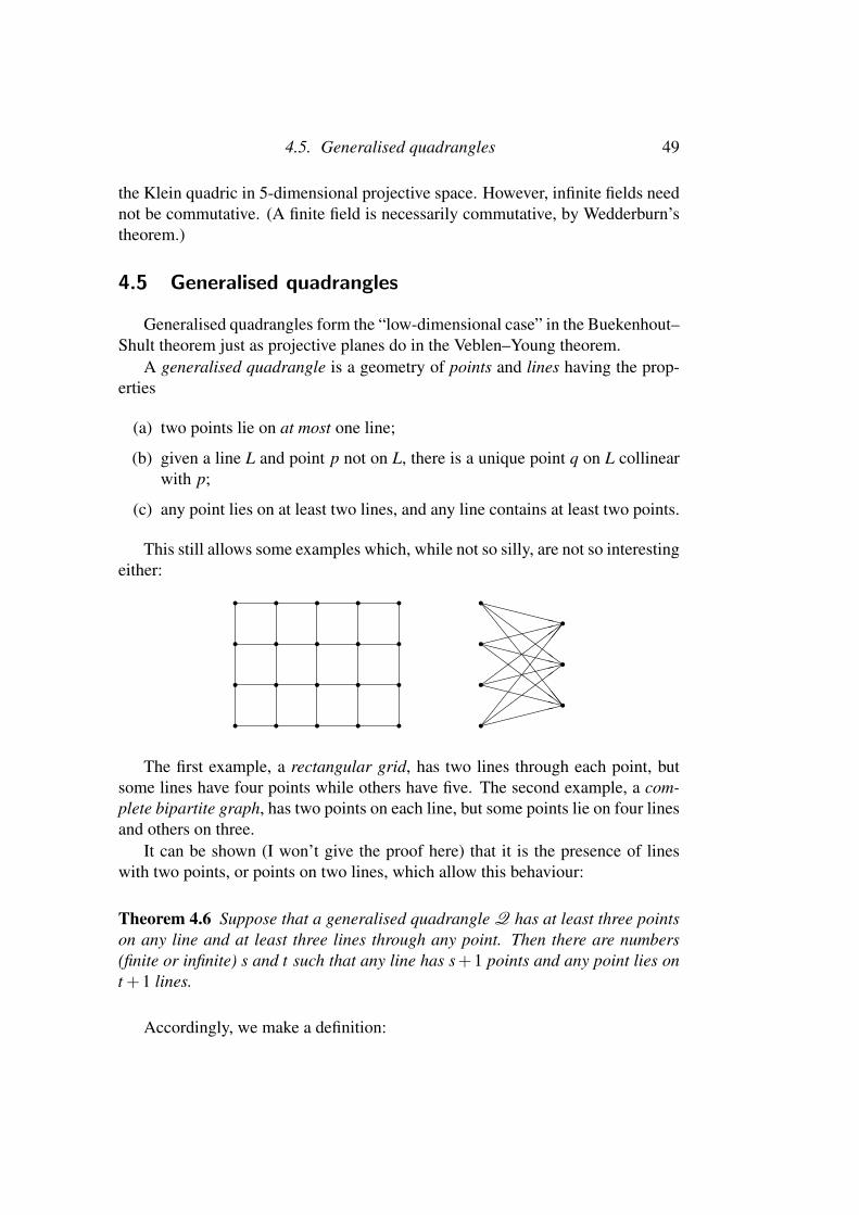
4.5. Generalised quadrangles 49
the Klein quadric in 5-dimensional projective space. However, infinite fields neednot be commutative. (A finite field is necessarily commutative, by Wedderburn’stheorem.)
4.5 Generalised quadrangles
Generalised quadrangles form the “low-dimensional case” in the Buekenhout–Shult theorem just as projective planes do in the Veblen–Young theorem.
A generalised quadrangle is a geometry of points and lines having the prop-erties
(a) two points lie on at most one line;
(b) given a line L and point p not on L, there is a unique point q on L collinearwith p;
(c) any point lies on at least two lines, and any line contains at least two points.
This still allows some examples which, while not so silly, are not so interestingeither:
r r r r rr r r r rr r r r rr r r r r
rrrr
rrr
������
������
�����
�
������
������
��������
XXXXXX
XXXXXX
XXXXXX
ZZZZZZ
ZZZZZZ
\\\\\\\\
The first example, a rectangular grid, has two lines through each point, butsome lines have four points while others have five. The second example, a com-plete bipartite graph, has two points on each line, but some points lie on four linesand others on three.
It can be shown (I won’t give the proof here) that it is the presence of lineswith two points, or points on two lines, which allow this behaviour:
Theorem 4.6 Suppose that a generalised quadrangle Q has at least three pointson any line and at least three lines through any point. Then there are numbers(finite or infinite) s and t such that any line has s+1 points and any point lies ont +1 lines.
Accordingly, we make a definition:

50 Chapter 4. Polar spaces
Definition A generalised quadrangle Q has parameters (s, t) if every line hass+1 points and every point lies on t +1 lines.
Thus we see that a rectangular grid has parameters if and only if it is square;and a complete bipartite graph has parameters if and only if the two parts of thepartition have equal size. Any generalised quadrangle not of one of these formsnecessarily has parameters.
There is a famous open problem here. Can we have a generalised quadranglewith parameters (s, t), where s is finite and s > 1, while t is infinite? It is knownthat this is not possible for s = 2, s = 3, and s = 4, though the arguments for thethree cases are very different and the degree of difficulty increases rapidly. Forlarger values of s, the problem is open. We will look at the case s = 2 shortly.
Theorem 4.7 Let Q be a generalised quadrangle with parameters (s, t). Then
(a) The number of points in Q is (s+ 1)(st + 1), and the number of lines is(t +1)(st +1).
(b) The point graph of Q, whose vertices are the points of Q, two verticesadjacent if they are collinear, is strongly regular, with parameters((s+1)(st +1),(t +1)s,s−1, t +1).
(c) A dual statement (with s and t exchanged) holds for the line graph of Q,whose vertices are the lines, two vertices adjacent if they intersect in a point.
Proof We prove (a) and (b) together. Take a point p, and let A(p) be the setof points collinear with p and B(p) the set not collinear. Then p lies on t + 1lines, each with s further points, and there are no overlaps among these points; so|A(p)|= (t +1)s is the number of neighbours of p.
Each neighbour q of p is joined to the s−1 further points on the line pq, andto no other points in A(p) (since the geometry contains no triangles). So there are(t +1)s−1− (s−1) = ts edges from q to points in B(p). On the other hand, eachpoint r ∈ B(p) is joined to one point on each of the t + 1 lines containing p; sop and r have t + 1 common neighbours. This shows the strong regularity of thegraph, and gives the stated parameters. Also, counting edges from A(p) to B(p),we have
|A(p)| · st = |B(p)| · (t +1),
and using |A(p)|= (t +1)s we get |B(p)|= s2t. So the total number of vertices is1+(t +1)s+ s2t = (s+1)(st +1), as required.
Part (c) is proved (and the number of lines counted) by a similar argumentwith the roles of points and lines reversed, or more simply by observing that thedual of Q (the geometry whose points are the lines of Q and whose lines are thepencils of lines of Q through a point, is a generalised quadrangle with parameters(t,s).

4.6. Generalised polygons 51
We now turn our attention to the case s = 2.
Theorem 4.8 Let Q be a (possibly degenerate) generalised quadrangle with threepoints on any line. Then the point graph of Q has the strong triangle property.Hence, if Q has parameters (2, t), then t = 1, 2 or 4.
Proof A line in Q corresponds to a triangle in the point graph; the second axiomfor a generalised quadrangle shows that any further vertex is joined to a uniquevertex in such a triangle. Thus the Strong Triangle Property holds. So the graph isnull, a Friendship graph, or one of our three exceptions. The null and Friendshipgraphs are degenerate (the first has no lines, and the second has points lying ononly one line); the other three cases give the three values of t in the theorem.
Remark A generalised quadrangle with three points on a line is equivalent toa graph with the strong triangle property. We saw while discussing that theoremthat necessarily t = 1, 2 or 4.
More generally, it is known that the parameters (s, t) of a generalised quad-rangle satisfy t ≤ s2 if s > 1, and dually s ≤ t2 if t > 1 (provided that s and t arefinite!).
There is a rather limited range of parameters for which generalised quadran-gles are known to exist. The following list includes all known examples. In thelist, q denotes a prime power.
• s = 1 (regular complete bipartite graphs);
• t = 1 (square grids);
• (s, t) = (q,q), (q,q2), (q2,q), (q2,q3), q3,q2);
• (s, t) = (q−1,q+1) or (q+1,q−1).
4.6 Generalised polygons
Generalised polygons are a class of geometries introduced by the Belgian ge-ometer Jacques Tits (winner of the Abel prize along with John Thompson a fewyears ago). They bear a similar relation to a more general class of things calledbuildings as projective planes do to projective spaces.
We now work towards the definition of a generalised n-gon, via a short detour.We have several times considered structures with points and lines, or points
and blocks. Sometimes (as with projective planes) we have considered a dualobject, where lines become points and points become lines. We need a way ofthinking about these which treats points and lines on the same footing.
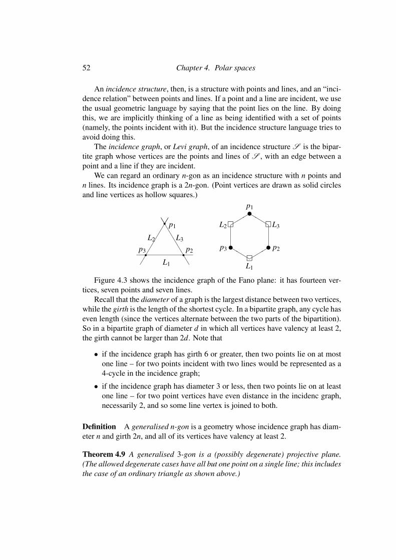
52 Chapter 4. Polar spaces
An incidence structure, then, is a structure with points and lines, and an “inci-dence relation” between points and lines. If a point and a line are incident, we usethe usual geometric language by saying that the point lies on the line. By doingthis, we are implicitly thinking of a line as being identified with a set of points(namely, the points incident with it). But the incidence structure language tries toavoid doing this.
The incidence graph, or Levi graph, of an incidence structure S is the bipar-tite graph whose vertices are the points and lines of S , with an edge between apoint and a line if they are incident.
We can regard an ordinary n-gon as an incidence structure with n points andn lines. Its incidence graph is a 2n-gon. (Point vertices are drawn as solid circlesand line vertices as hollow squares.)
��������
TTTTTTTT
r rr
L1
L2 L3
p3 p2
p1
�L1
up3
�L2
up1
�L3
up2"""
"""
bbb
bbb
Figure 4.3 shows the incidence graph of the Fano plane: it has fourteen ver-tices, seven points and seven lines.
Recall that the diameter of a graph is the largest distance between two vertices,while the girth is the length of the shortest cycle. In a bipartite graph, any cycle haseven length (since the vertices alternate between the two parts of the bipartition).So in a bipartite graph of diameter d in which all vertices have valency at least 2,the girth cannot be larger than 2d. Note that
• if the incidence graph has girth 6 or greater, then two points lie on at mostone line – for two points incident with two lines would be represented as a4-cycle in the incidence graph;
• if the incidence graph has diameter 3 or less, then two points lie on at leastone line – for two point vertices have even distance in the incidenc graph,necessarily 2, and so some line vertex is joined to both.
Definition A generalised n-gon is a geometry whose incidence graph has diam-eter n and girth 2n, and all of its vertices have valency at least 2.
Theorem 4.9 A generalised 3-gon is a (possibly degenerate) projective plane.(The allowed degenerate cases have all but one point on a single line; this includesthe case of an ordinary triangle as shown above.)
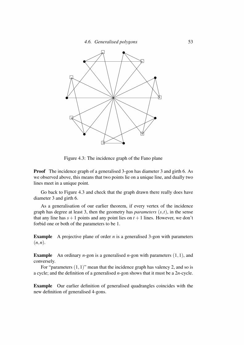
4.6. Generalised polygons 53
.
..............................................................................................................................................................
..............................................................................................................................................................................................................................................................................................................................................................................................................................
.
.............................................................................................................................................................
........................
........................
........................
........................
........................
........................
........................
........................
........................
........................
........................
........................
........................
........................
........................
........................
........................
........................
........................
........................
........................
........................
........................
........................
........................
........................
........................
...............
.
............................................
............................................
............................................
.........................
........................
........................
........................
........................
........................
........................
........................
........................
........................
........................
........................
........................
........................
........................
........................
........................
........................
.......
...............................................................................................................................................................................................................................................................................................................................................................................................................................................................................................................................................................................................................................................................................................................................
.
..............................................................................................................................................................
.......................................................................................................................................................................................................................................................................................................................................................................................................................................................
............................................
............................................
............................................
............................................
............................................
............................................
............................................
............................................
............................................
............................................
............................................
............................................
............................................
............................................
............................................
........................................
.
........................
........................
........................
........................
........................
........................
.....
............................................
............................................
............................................
............................................
............................................
............................................
............................................
............................................
............................................
..........................................
............................................................................................................................................................................................................................................................................................................................................................................................................................................................................................................................................................................................................................................................................................................................
.
......................................................................................................................................................................................................................................................................................................................................................................................................................................................
...............................................................................................................................................................................................................................................................................................................................................................................................................................................................................................................................................................................................................................................................................................................................
.
.....................................................................................................................................................
.......................................................................................................................................................................................................................................................................................................................................................................................................................................................
.......................................................................................................................................................................................................................................................................................................................................................................................................................................................................................................................................................................................................................................................................................
�
�
�
�
�
�
�
u
u
u
u
u
u
u
Figure 4.3: The incidence graph of the Fano plane
Proof The incidence graph of a generalised 3-gon has diameter 3 and girth 6. Aswe observed above, this means that two points lie on a unique line, and dually twolines meet in a unique point.
Go back to Figure 4.3 and check that the graph drawn there really does havediameter 3 and girth 6.
As a generalisation of our earlier theorem, if every vertex of the incidencegraph has degree at least 3, then the geometry has parameters (s, t), in the sensethat any line has s+1 points and any point lies on t +1 lines. However, we don’tforbid one or both of the parameters to be 1.
Example A projective plane of order n is a generalised 3-gon with parameters(n,n).
Example An ordinary n-gon is a generalised n-gon with parameters (1,1), andconversely.
For “parameters (1,1)” mean that the incidence graph has valency 2, and so isa cycle; and the definition of a generalised n-gon shows that it must be a 2n-cycle.
Example Our earlier definition of generalised quadrangles coincides with thenew definition of generalised 4-gons.

54 Chapter 4. Polar spaces
Proposition 4.10 If a generalised n-gon with n odd has parameters (s, t), thens = t.
Proof Take two vertices at maximum distance in the incidence graph. One is apoint p, and the other a line L. Now any point on L has a unique path to p oflength n−1, whose penultimate step is a line on p; and in reverse, any line on phas a unique path to L of length n−1, whose penultimate step is a point on L. Sothere is a bijection between lines through p and points on L.
The diagram shows the case n = 3. The lines through p are matched to thepoints on L by incidence. Note that this case refers to projective planes, which wehave seen before.
rrrrrr
����
�����
((((((((
(
hhhhhhhhhPPPPPPPPP
p L
The most important theorem about generalised polygons is the Feit–HigmanTheorem, proved in 1964.
Theorem 4.11 A finite generalised n-gon G with n≥ 3 and parameters (s, t) canexist only in the following cases:
(a) s = t = 1 (G is an ordinary n-gon);
(b) n = 3, 4, 6, 8 or 12 (and if n = 12, then s = 1 or t = 1).
The proof uses the eigenvalue techniques we have used often in this course. Iwill prove one special case of the theorem.
Theorem 4.12 A generalised 5-gon with parameters (s, t) exists only if s = t = 1.
Proof Suppose that G is a generalised 5-gon with parameters (s, t). Since 5 isodd, we know that s = t. Let G be the point graph of G .
We claim that G is a strongly regular graph with parameters (s4+ s3+ s2+ s+1,s(s+1),s−1,1).
Take a point p. This lies on s+ 1 lines, each containing s further points, andwithout overlap. So k = s(s+1).
Since the graph has no triangles, a neighbour q of p is joined to the s− 1further points on the line pq and no other neighbours of p. So λ = s−1.

4.6. Generalised polygons 55
Let r be a non-neighbour of p. Then the distance from p to r in the incidencegraph is 4. (It cannot be greater, since the diameter is 5; and it cannot be less,since r is not collinear with p.) So there is at least one point joined to both p andr. But there cannot be more than one, since the existence of two such points a andb would create either a triangle or a quadrangle in G , hence a circuit of length 6or 8 in the incidence graph. So µ = 1.
We calculate the number of vertices in the usual way.Now we apply the eigenvalue conditions. The adjacency matrix A of G sat-
isfies A2 = s(s+ 1)I +(s− 1)A+(J− I−A). So it has eigenvalue k = s(s+ 1)with multiplicity 1. The other eigenvalues satisfy θ 2 = s(s+1)+(s−1)θ−1−θ ,giving
θ = 12(s−2± s
√5).
Since both eigenvalues are irrational, their multiplicities must be equal, and musteach be 1
2s(s3 + s2 + s+1). Thus the equation Trace(A) = 0 gives
s(s+1)+ 12s(s+1)(s2 +1)(s−2) = 0.
This equation is satisfied when s = 1.But if s≥ 2, then s(s+1)> 0 and 1
2s(s+1)2(s−2)≥ 0, so the equation cannothold.
Remark An alternative way to finish the proof goes as follows. We saw in ourdiscussion of strongly regular graphs that, if the eigenvalues of A are irrational,then we are in Type 1, where n = 4µ +1 holds. Here, µ = 1, so n = 5.

Index
adjacency, 1adjacency matrix, 3alternating bilinear form, 42association scheme, 15
bilinear form, 42bipartite graph, 3Buekenhout–Shult Theorem, 48
Chang graph, 15Clebsch graph, 17complement, 3complete bipartite graph, 3complete graph, 3complete multipartite graph, 15connected graph, 3Conway group, 25Coxeter–Dynkin diagram, 31cube, 18cycle, 3
degree, 3design, 23diameter, 3directed edges, 2distance, 3dodecahedral graph, 17duality, 9
edges, 1
Feit–Higman Theorem, 54forest, 3Friendship Theorem, 1, 26Frobenius map, 47
generalised pentagon, 54generalised polygon, 52girth, 3graph, 1
bipartite, 3complete, 3complete bipartite, 3complete multipartite, 15connected, 3null, 3regular, 3square lattice, 15strongly regular, 14triangular, 15
Hamming distance, 18Hamming weight, 18Hermitian form, 47Higman, Graham, 25Hoffman–Singleton graph, 7
incidence graph, 52incidence structure, 52
Krein condition, 27
56
Index 57
Levi graph, 52line, 8line graph, 3loops, 2
McLaughlin graph, 25metric space, 3Moore graph, 7multiple edges, 2
neighbourhood, 2non-degenerate bilinear form, 42non-singular quadratic form, 43null graph, 3
orthogonal matrix, 9outer automorphism of S6, 13
Paley graph, 24parameters, 50Party Theorem, 21path, 3Perron–Frobenius Theorem, 32Petersen graph, 7, 17point, 8polar space, 48polarisation, 43polarity, 9projective plane, 8, 53projective space, 40
quadratic form, 43
radical, 42Ramsey number, 22Ramsey’s Theorem, 22reflexive bilinear form, 42regular graph, 3regular two-graph, 23, 26
Schlafli graph, 17self-dual, 9sesquilinear form, 47
Shrikhande graph, 15simple graph, 1square lattice graph, 15strong triangle property, 26strongly regular graph, 14symmetric bilinear form, 42symmetric matrix, 9
tree, 3triangle property, 44triangular graph, 15
valency, 3Veblen–Young theorem, 41vertices, 1
Wedderburn’s Theorem, 49Whitney’s Theorem, 39Witt design, 25Witt index, 48