Eigenvalues and Eigenvectorsstecher/LinearAlgebraPdfFiles/chapterFive.pdf · The eigenvalue 2 has...
28
Chapter 5 Eigenvalues and Eigenvectors In this chapter we return to the study of linear transformations that we started in Chapter 3. The ideas presented here are related to finding the “simplest” matrix representation for a fixed linear transformation. As you recall, a matrix representation is determined once the bases for the two vector spaces are picked. Thus our problem is how to pick these bases. 5.1 What is an Eigenvector? Before defining eigenvectors and eigenvalues let us look at the linear transfor- mation L, from R 2 to R 2 , whose matrix representation is A = 2 0 0 3 We cannot compute L(x 1 ,x 2 ) until we specify which basis G we used. Let’s assume that G = {g 1 ,g 2 }. Then we know that L(g 1 )=2g 1 +0g 2 =2g 1 and L(g 2 )=0g 1 +3g 2 =3g 2 . Thus, L(g k ) just multiplies g k by the corresponding element in the main diagonal of A. Figure 5.1 illustrates this. If x = x 1 g 1 + x 2 g 2 , then L(x)=2x 1 g 1 +3x 2 g 2 . Since L multiplies each basis vector by some constant, it is extremely easy to compute and visualize what the linear transformation does to R 2 . In fact, since scalar multiplication is the simplest linear transformation possible, we would like to be able to do the following. Given a linear transformation L from R n to R n , find a basis F = {f 1 ,...,f n } such that L(f k )= λ k f k for k =1, 2,...,n, that is, find n linearly independent vectors upon which L acts as scalar multiplication. Unfortunately, it is not always possible to do this. There are, however, large classes of linear transfor- mations for which it is possible to find such a set of vectors. These vectors are called eigenvectors and the scalar multipliers λ k are called the eigenvalues of L. The reader should note that the terms characteristic 173
Transcript of Eigenvalues and Eigenvectorsstecher/LinearAlgebraPdfFiles/chapterFive.pdf · The eigenvalue 2 has...
Chapter 5
Eigenvalues and
Eigenvectors
In this chapter we return to the study of linear transformations that we startedin Chapter 3. The ideas presented here are related to finding the “simplest”matrix representation for a fixed linear transformation. As you recall, a matrixrepresentation is determined once the bases for the two vector spaces are picked.Thus our problem is how to pick these bases.
5.1 What is an Eigenvector?
Before defining eigenvectors and eigenvalues let us look at the linear transfor-mation L, from R2 to R2, whose matrix representation is
A =
[
2 00 3
]
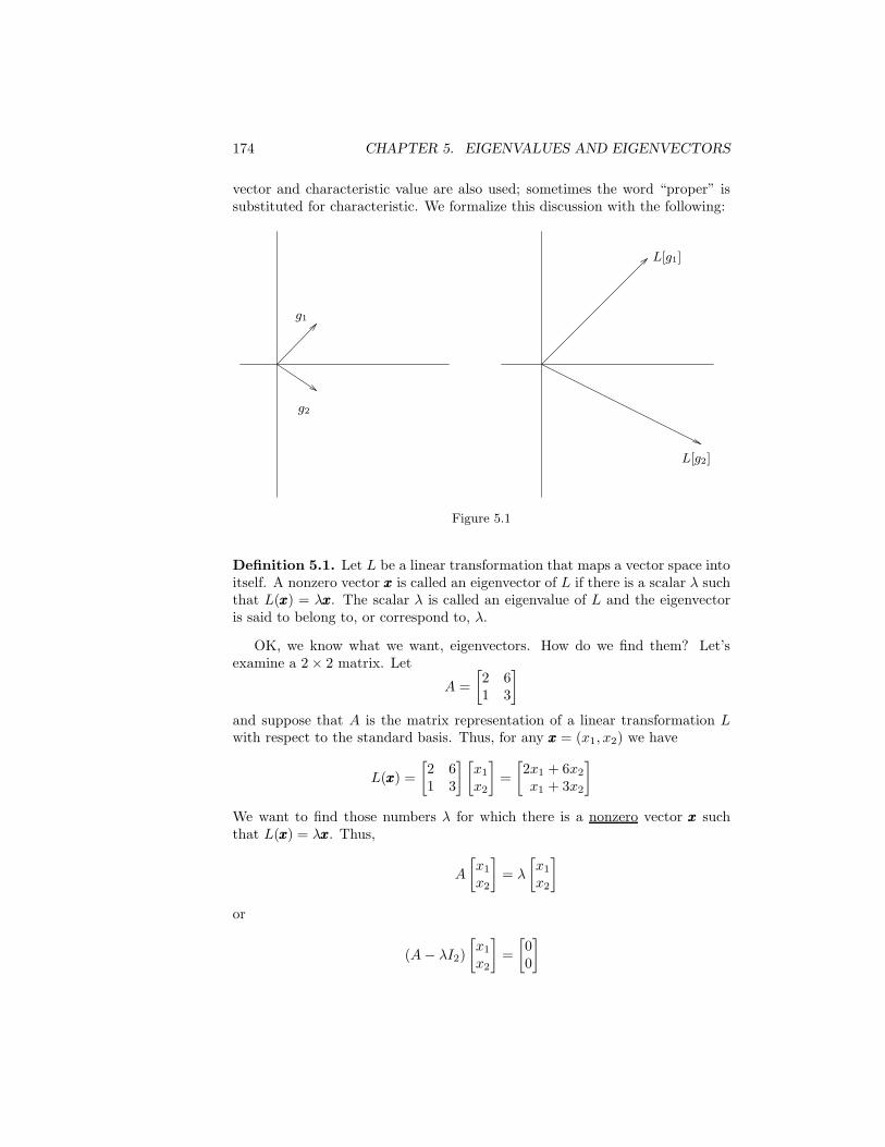
We cannot compute L(x1, x2) until we specify which basis G we used. Let’sassume that G = {ggg1, ggg2}. Then we know that L(ggg1) = 2ggg1 + 0ggg2 = 2ggg1 andL(ggg2) = 0ggg1 + 3ggg2 = 3ggg2. Thus, L(gggk) just multiplies gggk by the correspondingelement in the main diagonal of A. Figure 5.1 illustrates this. If xxx = x1ggg1 +x2ggg2, then L(xxx) = 2x1ggg1 + 3x2ggg2. Since L multiplies each basis vector bysome constant, it is extremely easy to compute and visualize what the lineartransformation does to R2. In fact, since scalar multiplication is the simplestlinear transformation possible, we would like to be able to do the following.
Given a linear transformationL from Rn to Rn, find a basis F = {fff1, . . . , fffn}such that L(fffk) = λkfffk for k = 1, 2, . . . , n, that is, find n linearly independentvectors upon which L acts as scalar multiplication. Unfortunately, it is notalways possible to do this. There are, however, large classes of linear transfor-mations for which it is possible to find such a set of vectors.
These vectors are called eigenvectors and the scalar multipliers λk are calledthe eigenvalues of L. The reader should note that the terms characteristic
173
174 CHAPTER 5. EIGENVALUES AND EIGENVECTORS
vector and characteristic value are also used; sometimes the word “proper” issubstituted for characteristic. We formalize this discussion with the following:
g1
g2
L[g1]
L[g2]
Figure 5.1
Definition 5.1. Let L be a linear transformation that maps a vector space intoitself. A nonzero vector xxx is called an eigenvector of L if there is a scalar λ suchthat L(xxx) = λxxx. The scalar λ is called an eigenvalue of L and the eigenvectoris said to belong to, or correspond to, λ.
OK, we know what we want, eigenvectors. How do we find them? Let’sexamine a 2× 2 matrix. Let
A =
[
2 61 3
]
and suppose that A is the matrix representation of a linear transformation Lwith respect to the standard basis. Thus, for any xxx = (x1, x2) we have
L(xxx) =
[
2 61 3
] [
x1x2
]
=
[
2x1 + 6x2x1 + 3x2
]
We want to find those numbers λ for which there is a nonzero vector xxx suchthat L(xxx) = λxxx. Thus,
A
[
x1x2
]
= λ
[
x1x2
]
or
(A− λI2)
[
x1x2
]
=
[
00
]

5.1. WHAT IS AN EIGENVECTOR? 175
Hence, we are looking for those numbers λ for which the equation (A−λI2)xxx = 000has a nontrivial solution. But this happens if and only if det(A−λI2) = 0. Forthis particular A we have
det(A− λI2) = det
[
2− λ 61 3− λ
]
= (2− λ)(3 − λ) − 6
= λ2 − 5λ = λ(λ− 5)
The only values of λ that satisfy the equation det(A − λI2) = 0 are λ = 0 andλ = 5. Thus the eigenvalues of L are 0 and 5. An eigenvector of 5, for example,will be any nonzero vector xxx in the kernel of A− 5I2.
In the following pages when we talk about finding the eigenvalues and eigen-vectors of some n×nmatrix A, what we mean is that A is the matrix representa-tion, with respect to the standard basis in Rn, of a linear transformation L, andthe eigenvalues and eigenvectors of A are just the eigenvalues and eigenvectorsof L.
Example 1. Find the eigenvalues and eigenvectors of the matrix
[
2 61 3
]
From the above discussion we know that the only possible eigenvalues of A are0 and 5.
λ = 0: We want xxx = (x1, x2) such that
([
2 61 3
]
− 0
[
1 00 1
])[
x1x2
]
=
[
00
]
The coefficient matrix of this system is
[
2 61 3
]
, and it is row equivalent to the
matrix
[
1 30 0
]
. The solutions to this homogeneous equation satisfy x1 = −3x2.
Therefore, ker(A − 0I2) = S[(−3, 1)], and any eigenvector of A correspondingto the eigenvalue 0 is a nonzero multiple of (−3, 1). As a check we compute
A
[
−31
]
=
[
2 61 3
] [
−31
]
=
[
00
]
= 0
[
−31
]
λ = 5: We want to find those vectors xxx such that (A− 5I2)xxx = 000. This leadsto the equation
([
2 61 3
]
− 5
[
1 00 1
])[
x1x2
]
=
[
00
]
The coefficient matrix of this system,
[
−3 61 −2
]
, is row equivalent to the matrix[
1 −20 0
]
. Any solution of this system satisfies x1 = 2x2. Hence, ker(A −
176 CHAPTER 5. EIGENVALUES AND EIGENVECTORS
5I2) = S[(2, 1)]. All eigenvectors corresponding to the eigenvalue λ = 5 must benonzero multiples of (2,1). Checking to see that (2,1) is indeed an eigenvectorcorresponding to 5, we have
A
[
21
]
=
[
2 61 3
] [
21
]
=
[
105
]
= 5
[
21
]
�
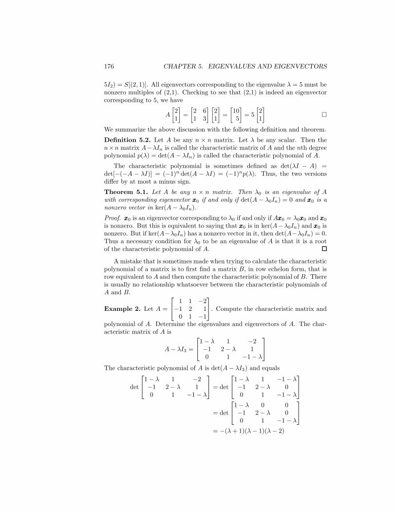
We summarize the above discussion with the following definition and theorem.
Definition 5.2. Let A be any n × n matrix. Let λ be any scalar. Then then×n matrix A−λIn is called the characteristic matrix of A and the nth degreepolynomial p(λ) = det(A− λIn) is called the characteristic polynomial of A.
The characteristic polynomial is sometimes defined as det(λI − A) =det[−(−A − λI)] = (−1)n det(A − λI) = (−1)np(λ). Thus, the two versionsdiffer by at most a minus sign.
Theorem 5.1. Let A be any n × n matrix. Then λ0 is an eigenvalue of Awith corresponding eigenvector xxx0 if and only if det(A− λ0In) = 0 and xxx0 is anonzero vector in ker(A− λ0In).
Proof. xxx0 is an eigenvector corresponding to λ0 if and only if Axxx0 = λ0xxx0 and xxx0is nonzero. But this is equivalent to saying that xxx0 is in ker(A−λ0In) and xxx0 isnonzero. But if ker(A−λ0In) has a nonzero vector in it, then det(A−λ0In) = 0.Thus a necessary condition for λ0 to be an eigenvalue of A is that it is a rootof the characteristic polynomial of A.
A mistake that is sometimes made when trying to calculate the characteristicpolynomial of a matrix is to first find a matrix B, in row echelon form, that isrow equivalent to A and then compute the characteristic polynomial of B. Thereis usually no relationship whatsoever between the characteristic polynomials ofA and B.
Example 2. Let A =
1 1 −2−1 2 10 1 −1
. Compute the characteristic matrix and
polynomial of A. Determine the eigenvalues and eigenvectors of A. The char-acteristic matrix of A is
A− λI3 =
1− λ 1 −2−1 2− λ 10 1 −1− λ
The characteristic polynomial of A is det(A− λI3) and equals
det
1− λ 1 −2−1 2− λ 10 1 −1− λ
= det
1− λ 1 −1− λ−1 2− λ 00 1 −1− λ
= det
1− λ 0 0−1 2− λ 00 1 −1− λ
= −(λ+ 1)(λ− 1)(λ− 2)

5.1. WHAT IS AN EIGENVECTOR? 177
Thus, the eigenvalues of A are −1, 1, and 2. We determine the eigenvectors ofA by finding the nonzero vectors in ker(A− λ0I3), for λ0 = −1, 1, and 2.
λ = −1: The matrix A− (−1)I3 equals
2 1 −2−1 3 10 1 0
and it is row equiva-
lent to the matrix
1 0 −10 1 00 0 0
. This implies that ker(A+I3) equals S[(1, 0, 1)].
One easily checks that A(1, 0, 1)T = (−1)(1, 0, 1)T .
λ = 1: A − I3 =
0 1 −2−1 1 10 1 −2
, and this matrix is row equivalent to
0 1 −21 0 −30 0 0
. Clearly ker(A − I3) = S[(3, 2, 1)], and a quick calculation shows
that A(3, 2, 1)T = (3, 2, 1)T .
λ = 2: A − 2I3 =
−1 1 −2−1 0 10 1 −3
. This matrix is row equivalent to
1 0 −10 1 −30 0 0
. Thus, ker(A − 2I3) = S[(1, 3, 1)]. Computing A(1, 3, 1)T , we
see that it equals 2(1, 3, 1)T . �
If A is an n× n matrix, we’ve defined the characteristic polynomial p(λ) ofA to be det(A − λIn). If λ1, λ2, . . . , λq are the distinct roots of p(λ), then wemay write
p(λ) = (−1)n(λ− λ1)m1(λ− λ2)
m2 . . . (λ − λq)mq
wherem1+m2+ · · ·+mq = n. The multiplicity of an eigenvalue is the exponentcorresponding to that eigenvalue. Thus, the multiplicity of λ1 is m1, that of λ2
beingm2, etc. For example, if A equals
2 1 0 00 2 1 00 0 2 20 0 0 4
, then p(λ) = (λ−2)3(λ−
4). The eigenvalue 2 has multiplicity 3 while the eigenvalue 4 has multiplicity1.
One last bit of terminology: When we wish to talk about all the eigenvectorsassociated with one eigenvalue we use the term eigenspace. Thus, in Example 2the eigenspace of the eigenvalue (−1) is just ker(A− (−1)I). In general, if L isany linear transformation from a vector space into itself and λ0 is an eigenvalueof L, the eigenspace of λ0 is ker(L−λ0I). That is, the eigenspace of λ0 consistsof all its eigenvectors plus the zero vector. Note that the zero vector is never aneigenvector.
We’ve seen how to compute the eigenvalues of a linear transformation if thelinear transformation is matrix multiplication. What do we do in the more
178 CHAPTER 5. EIGENVALUES AND EIGENVECTORS
abstract setting when L : V → V ? Well, in Chapter 3 we saw that once wefix a basis F = {fff1, . . . , fffn} of V , we have a matrix representation, A, of L.Moreover, L(xxx) = λxxx for some nonzero vector xxx and scalar λ if and only ifA[xxx]F = λ[xxx]F . Thus, λ is an eigenvalue of L if and only if det(A−λI) = 0, andker(A−λI) has a nonzero vector and the nonzero vectors in ker(A−λI) are thecoordinates, with respect to the basis F , of the nonzero vectors in ker(L− λI).What this means is that we may calculate the eigenvalues and eigenvectorsof L by calculating the eigenvalues and eigenvectors of any one of its matrixrepresentations.
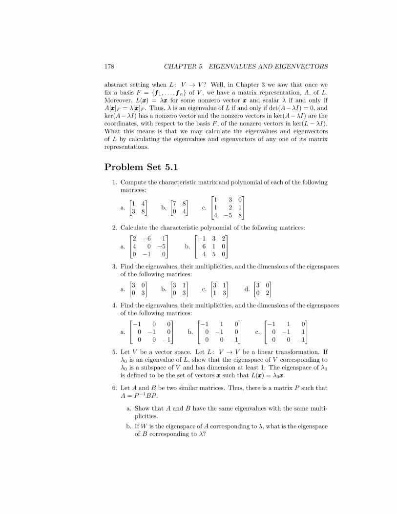
Problem Set 5.1
1. Compute the characteristic matrix and polynomial of each of the followingmatrices:
a.
[
1 43 8
]
b.
[
7 80 4
]
c.
1 3 01 2 14 −5 8
2. Calculate the characteristic polynomial of the following matrices:
a.
2 −6 14 0 −50 −1 0
b.
−1 3 26 1 04 5 0
3. Find the eigenvalues, their multiplicities, and the dimensions of the eigenspacesof the following matrices:
a.
[
3 00 3
]
b.
[
3 10 3
]
c.
[
3 11 3
]
d.
[
3 00 2
]
4. Find the eigenvalues, their multiplicities, and the dimensions of the eigenspacesof the following matrices:
a.
−1 0 00 −1 00 0 −1
b.
−1 1 00 −1 00 0 −1
c.
−1 1 00 −1 10 0 −1
5. Let V be a vector space. Let L : V → V be a linear transformation. Ifλ0 is an eigenvalue of L, show that the eigenspace of V corresponding toλ0 is a subspace of V and has dimension at least 1. The eigenspace of λ0is defined to be the set of vectors xxx such that L(xxx) = λ0xxx.
6. Let A and B be two similar matrices. Thus, there is a matrix P such thatA = P−1BP .
a. Show that A and B have the same eigenvalues with the same multi-plicities.
b. IfW is the eigenspace of A corresponding to λ, what is the eigenspaceof B corresponding to λ?

5.1. WHAT IS AN EIGENVECTOR? 179
7. Let A be an n × n matrix. Let p(λ) = det(A − λIn) be its characteristicpolynomial. Then if λ1, λ2, . . . , λn are the roots of p(λ), we may write
p(λ) = (−1)n(λ− λ1)(λ − λ2) . . . (λ− λn)
= (−1)n[λn − c1λn−1 + · · ·+ (−1)ncn]
a. Assume A is a 2 × 2 matrix, A = [ajk]. Then p(λ) = λ2 − c1λ + c2.Show that c2 = det(A) = λ1λ2 and c1 = λ1 + λ2 = a11 + a22.
b. Assume A = [ajk] is a 3 × 3 matrix. Then p(λ) = −(λ3 − c1λ2 +
c2λ − c3). Show that c1 = λ1 + λ2 + λ3 = a11 + a22 + a33 and thatc3 = det(A) = λ1λ2λ3.
c. Generalize parts a and b to n× n matrices.
8. If A is an n × n matrix, A = [ajk], we define the trace of A = Tr(A) =a11 + a22 + · · ·+ ann. Show that the following are true for any two n× nmatrices A and B:
a. Tr(A+B) = Tr(A) + Tr(B)
b. Tr(AB) = Tr(BA)
c. Tr(A) = Tr(AT )
d. Show that if A and B are similar matrices, Tr(A) = Tr(B).
9. Let A be an n× n matrix and let p(λ) = det(A− λIn), the characteristicpolynomial of A. Then if λ1, λ2, . . . , λn are the roots of p(λ), we may write
p(λ) = (−1)n(λ− λ1)(λ − λ2) . . . (λ− λn)
= (−1)n[λn − c1λn−1 + · · ·+ (−1)ncn]
By p(A) we mean
p(A) = (−1)n[An − c1An−1 + · · ·+ (−1)ncnIn]
That is, wherever λ appears in p(λ), it is replaced by A. For each of thematrices in problem 1 compute p(A).
10. Let A =
[
0 22 0
]
. Show that the eigenvalues of A are ±2. Let xxx and yyy be
two eigenvectors corresponding to 2 and −2, respectively.
a. Show that Anxxx = 2nxxx and Anyyy = (−2)nyyy.
b. Let g(λ) = λn+c1λn−1+ · · ·+cn be an arbitrary polynomial. Define
the matrix g(A) by g(A) = An + c1An−1 + · · · + cnI. Show that
g(A)xxx = g(2)xxx and g(A)yyy = g(−2)yyy.
11. Let A be any n× n matrix. Suppose λ0 is an eigenvalue of A with xxx0 anyeigenvector corresponding to λ0. Let g(λ) be any polynomial in λ; defineg(A) as in problem 10. Show that g(A)xxx0 = g(λ0)xxx0.

180 CHAPTER 5. EIGENVALUES AND EIGENVECTORS
12. Let A =
[
0 −11 0
]
. As we saw in Chapter 3, this matrix represents a
rotation of 90 degrees about the origin. As such, we should not expectany eigenvectors. Why? Compute det(A − λI) and find all the roots ofthis polynomial. Show that there is no vector xxx in R2 such that Axxx = λxxxexcept for the zero vector. What happens if R2 is replaced by C2? Forwhich rotations in R2, if any, are there eigenvectors?
13. Find the eigenvalues and eigenspaces of the matrices below:
0 0 −3 4−2 2 −2 4−2 0 1 2−3 0 −3 7
4
3
4
30 2
2
3
2
30 1
−1 −1 0 3
−1
3−1
30 0
14. Let A =
[
d1 00 d2
]
.
a. Find the eigenvalues and eigenspaces of A.
b. Let p(λ) = det(A−λI). Show that p(A) = 022, the zero 2×2 matrix;cf. problem 10.
c. Assume that det(A) = d1d2 6= 0. Use the equation p(A) = 022 tocompute A−1, where p(λ) = det(A− λI).
15. Let A = [ajk] be any 2 × 2 matrix. Let p(λ) be its characteristic polyno-mial. Show that p(A) = 022. Assume that det(A) 6= 0 and show how tocompute A−1 using this information.
16. Let A be any n× n matrix and let p(λ) be its characteristic polynomial.The Hamilton–Cayley theorem states that p(A) = 0nn. Assuming thatdet(A) 6= 0, explain how one could compute A−1 by using the equationp(A) = 0nn.
17. Let A =
[
6 10 9
]
.
a. Find the eigenvalues of A.
b. For any constant c, find the eigenvalues of the matrix A− cI.
c. For any constant c, find the eigenvalues of the matrix cA.
18. Let A be any n×n matrix. Suppose the eigenvalues of A are {λ1, . . . , λn}.Let c be any constant.
a. Show that the eigenvalues of A− cI are {λ1 − c, . . . , λn − c}.b. What are the eigenvalues of cA?

5.1. WHAT IS AN EIGENVECTOR? 181
19. Let A = [ajk] be an invertible n × n matrix. Suppose that {λ1, . . . , λn}is the set of eigenvalues of A. Show that λj 6= 0 for j = 1, . . . , n. Thenshow that the eigenvalues of A−1 are the reciprocals of the λj . That is,if 2 is an eigenvalue of A, then 1
2 is an eigenvalue of A−1. How are theeigenvectors of A and A−1 related?
20. Let A be an n× n matrix. Suppose xxx0 is an eigenvector of A.
a. Show that xxx0 is an eigenvector of An for any n.
b. What is the eigenvalue of An for which xxx0 is the corresponding eigen-vector?
c. Show that xxx0 is an eigenvector of A− kI for any constant k.
d. What is the eigenvalue of A − kI for which xxx0 is the correspondingeigenvector?
21. Show that det(A−λI) = det(AT−λI) for any constant λ. Thus, A and AT
have the same characteristic polynomial, and hence the same eigenvalues.
22. Find a 2×2 matrixA for which A andAT do not have the same eigenspaces.
23. Find the eigenvalues, their multiplicities, and the dimensions of the cor-responding eigenspaces for each of the following matrices:
a.
1 1 0 00 1 0 00 0 1 00 0 0 1
b.
1 1 0 00 1 1 00 0 1 00 0 0 1
c.
1 1 0 00 1 1 00 0 1 10 0 0 1
24. Let A =
[
−1 31 1
]
. Define L : M22 → M22 by L[B] = AB for any B in
M22. Find the eigenvalues of L, their multiplicities, and the dimensionsof the eigenspaces.
25. Let A be any n×n matrix. Define L : Mnn → Mnn by L[B] = AB. Showthat λ is an eigenvalue of L if and only if λ is an eigenvalue of the matrixA. Remember that λ is an eigenvalue of A only if there exists a nonzeroxxx in Rn such that Axxx = λxxx.
26. Define L : P2 → P2 by L[ppp](t) = (1/t)´ t
0 ppp(s)ds. Find the eigenvalues,their multiplicities, and the dimensions of the eigenspaces.
27. Let A =
[
1 30 1
]
. Let B =
[
1 00 6
]
. Define L : M22 → M22 by
L[xxx] = Axxx + xxxB. Show that L is a linear transformation, and then findits eigenvalues, their multiplicities, and the corresponding eigenspaces.
182 CHAPTER 5. EIGENVALUES AND EIGENVECTORS
5.2 Diagonalization of Matrices
In the last section we stated that the eigenvalues of a matrix A are those rootsof the characteristic polynomial p(λ) = det(A − λI) for which ker(A − λI)contains more than just the zero vector. The fundamental theorem of algebrastates that every polynomial has at least one root. Thus, every matrix shouldhave at least one eigenvalue and a corresponding eigenvector. This argumenterroneously leads us to believe that every linear transformation L, from a vectorspace V into V , has at least one eigenvector and eigenvalue. This need not betrue when V is a real vector space, since multiplication by complex numbers isnot allowed, and the root of p(λ) = 0 that is guaranteed by the fundamental
theorem of algebra may be a complex number. The matrix
[
0 −11 0
]
is one such
example; cf. problem 12 in Section 5.1. The trouble with a complex numberbeing an eigenvalue is that our vector space may only allow multiplication byreal numbers. For example, if i represents the square root of −1 and xxx = (1, 2),a vector in R2, then ixxx = (i, 2i) makes sense, but it is no longer in R2. If ourvector space is C2, then, since multiplication by complex scalars is allowed, theabove problem does not arise.
Let’s step back and review what it is we want:
simple representations for linear transformations.
From this, we are led to the idea of eigenvectors and the realization that wewant not just one eigenvector, but a basis of eigenvectors. In fact, we have thefollowing theorem.
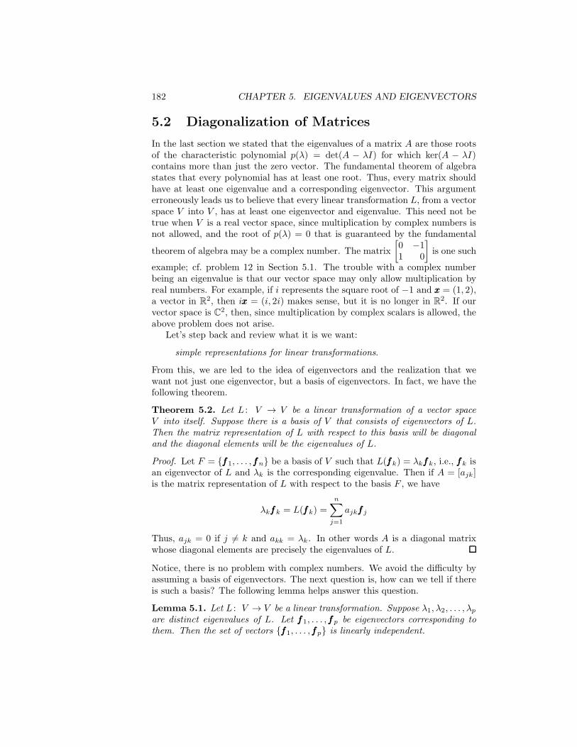
Theorem 5.2. Let L : V → V be a linear transformation of a vector spaceV into itself. Suppose there is a basis of V that consists of eigenvectors of L.Then the matrix representation of L with respect to this basis will be diagonaland the diagonal elements will be the eigenvalues of L.
Proof. Let F = {fff1, . . . , fffn} be a basis of V such that L(fffk) = λkfffk, i.e., fffk isan eigenvector of L and λk is the corresponding eigenvalue. Then if A = [ajk]is the matrix representation of L with respect to the basis F , we have
λkfffk = L(fffk) =
n∑
j=1
ajkfff j
Thus, ajk = 0 if j 6= k and akk = λk. In other words A is a diagonal matrixwhose diagonal elements are precisely the eigenvalues of L.
Notice, there is no problem with complex numbers. We avoid the difficulty byassuming a basis of eigenvectors. The next question is, how can we tell if thereis such a basis? The following lemma helps answer this question.
Lemma 5.1. Let L : V → V be a linear transformation. Suppose λ1, λ2, . . . , λpare distinct eigenvalues of L. Let fff1, . . . , fffp be eigenvectors corresponding tothem. Then the set of vectors {fff1, . . . , fffp} is linearly independent.

5.2. DIAGONALIZATION OF MATRICES 183
Proof. We prove that this set is linearly independent by an inductive process;that is, we show the theorem is true when p = 1 and 2 and then show how to gofrom p− 1 to p. Suppose p = 1: then the set in question is just {fff1}, and sincefff1 6= 0, it is linearly independent. Now suppose there are constants c1 and c2such that
000 = c1fff1 + c2fff2 (5.1)
Then we also have
000 = L(000) = L(c1fff1 + c2fff2)
= c1L(fff1) + c2L(fff2)
= c1λ1fff1 + c2λ2fff2 (5.2)
Multiplying (5.1) by λ1, and subtracting the resulting equation from (5.2), wehave
000 = c2(λ2 − λ1)fff2
Since fff2 6= 0 and λ2 6= λ1, we must have c2 = 0. This and (5.1) imply c1 = 0.Hence, {fff1, fff2} is linearly independent. Assume now that the set {fff1, . . . , fffp−1}is linearly independent and
000 = c1fff1 + c2fff2 + · · ·+ cp−1fffp−1 + cpfffp (5.3)
for some constants c1, . . . , cp. Then
000 = L[c1fff1 + · · ·+ cpfffp]
= c1L(fff1) + · · ·+ cpL(fffp)
= c1λ1fff1 + · · ·+ cpλpfffp (5.4)
Multiplying (5.3) by λp, and then subtracting from (5.4), we have
000 = c1(λ1 − λp)fff1 + c2(λ2 − λp)fff2 + · · ·+ cp−1(λp−1 − λp)fffp−1
Since the fffk’s, 1 ≤ k ≤ p − 1, are linearly independent we must have ck(λk −λp) = 0 for k = 1, 2, . . . , p− 1. But λp 6= λk; hence ck = 0, k = 1, 2, . . . , p− 1.Thus, (5.3) reduces to cpfffp = 000 and we conclude that cp = 0 also. This ofcourse means that our set of vectors is linearly independent.
Theorem 5.3. Let V be a real n-dimensional vector space. Let L be a lineartransformation from V into V . Suppose that the characteristic polynomial of Lhas n distinct real roots. Then L has a diagonal matrix representation.
Proof. Let the roots of the characteristic polynomial be λ1, λ2, . . . , λn. By hy-pothesis they are all different and real. Thus, for each j, ker(L − λjI) willcontain more than just the zero vector. Hence, each of these roots is an eigen-values, and if fff1, . . . , fffn is a set of associated eigenvectors, the previous lemmaensures that they form a linearly independent set. Since dim(V ) = n, they alsoform a basis for V . Theorem 5.2 guarantees that L does indeed have a matrixrepresentation that is diagonal.

184 CHAPTER 5. EIGENVALUES AND EIGENVECTORS
Note that if V in the above theorem is an n-dimensional complex vectorspace, we would not need to insist that the roots of the characteristic polynomialbe real.
Example 1. Let L be a linear transformation from R4 to R4 whose matrixrepresentation A with respect to the standard basis is
−3 0 2 −4−6 2 2 −54 0 −1 46 0 −2 7
Find a diagonal representation for L.
Solution. The characteristic polynomial p(λ) of L is
p(λ) = det
−3− λ 0 2 −4−6 2− λ 2 −54 0 −1− λ 46 0 −2 7− λ
= (2− λ) det
−3− λ 2 −44 −1− λ 46 −2 7− λ
= (2− λ) det
3− λ 0 3− λ4 −1− λ 46 −2 7− λ
= (2− λ) det
3− λ 0 04 −1− λ 06 −2 1− λ
= (−1− λ)(1 − λ)(2 − λ)(3 − λ)
Thus, the roots of p(λ) are −1, 1, 2, and 3. Since they are real and distinct,Theorem 5.3 guarantees that R4 will have a basis that consists of eigenvectorsof L. We next find one eigenvector for each of the eigenvalues.
λ = −1:
A− (−1)I =
−2 0 2 −4−6 3 2 −54 0 0 46 0 −2 8
is row equivalent to
1 0 0 10 1 0 10 0 1 −10 0 0 0
Thus, ker(A + I) = S[(−1,−1, 1, 1)], and fff1 = (−1,−1, 1, 1) is an eigenvectorcorresponding to −1.
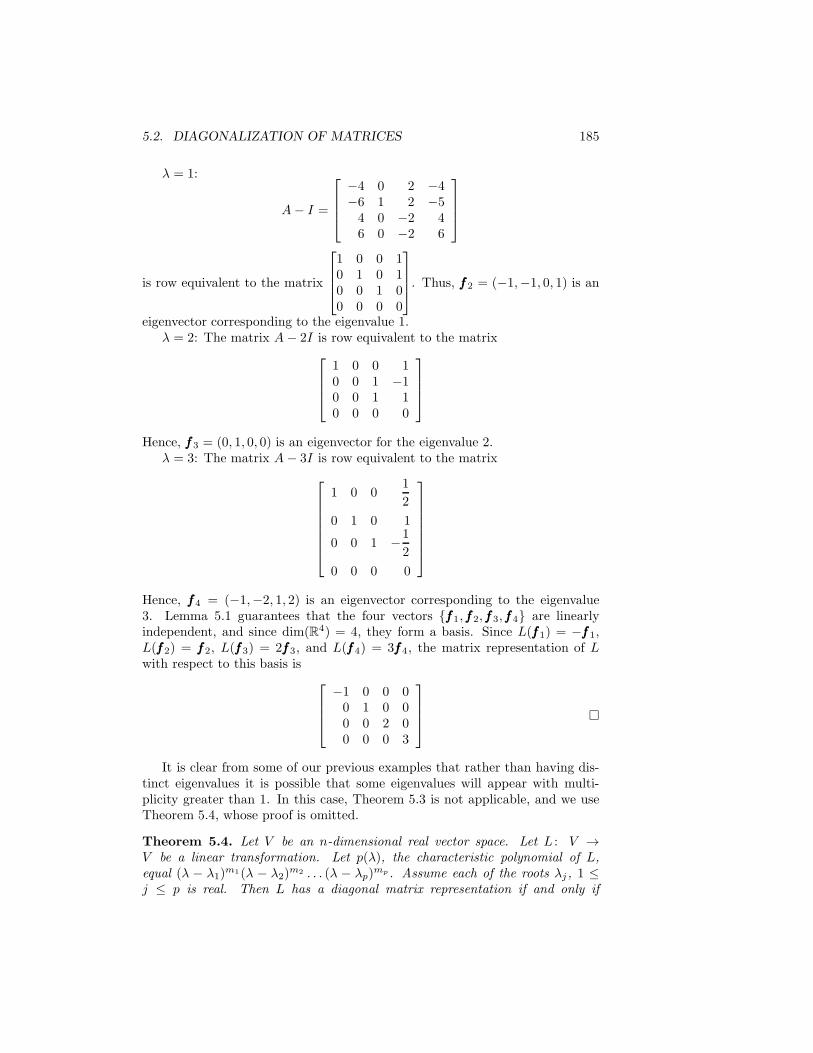
5.2. DIAGONALIZATION OF MATRICES 185
λ = 1:
A− I =
−4 0 2 −4−6 1 2 −54 0 −2 46 0 −2 6
is row equivalent to the matrix
1 0 0 10 1 0 10 0 1 00 0 0 0
. Thus, fff2 = (−1,−1, 0, 1) is an
eigenvector corresponding to the eigenvalue 1.λ = 2: The matrix A− 2I is row equivalent to the matrix
1 0 0 10 0 1 −10 0 1 10 0 0 0
Hence, fff3 = (0, 1, 0, 0) is an eigenvector for the eigenvalue 2.λ = 3: The matrix A− 3I is row equivalent to the matrix
1 0 01
2
0 1 0 1
0 0 1 −1
2
0 0 0 0
Hence, fff4 = (−1,−2, 1, 2) is an eigenvector corresponding to the eigenvalue3. Lemma 5.1 guarantees that the four vectors {fff1, fff2, fff3, fff4} are linearlyindependent, and since dim(R4) = 4, they form a basis. Since L(fff1) = −fff1,L(fff2) = fff2, L(fff3) = 2fff3, and L(fff4) = 3fff4, the matrix representation of Lwith respect to this basis is
−1 0 0 00 1 0 00 0 2 00 0 0 3
�
It is clear from some of our previous examples that rather than having dis-tinct eigenvalues it is possible that some eigenvalues will appear with multi-plicity greater than 1. In this case, Theorem 5.3 is not applicable, and we useTheorem 5.4, whose proof is omitted.
Theorem 5.4. Let V be an n-dimensional real vector space. Let L : V →V be a linear transformation. Let p(λ), the characteristic polynomial of L,equal (λ − λ1)
m1(λ − λ2)m2 . . . (λ − λp)
mp . Assume each of the roots λj , 1 ≤j ≤ p is real. Then L has a diagonal matrix representation if and only if

186 CHAPTER 5. EIGENVALUES AND EIGENVECTORS
dim(ker(A − λjI)) = mj for each of the eigenvalues λj ; that is, the number oflinearly independent solutions to the homogeneous equation (A−λjI)xxx = 000 mustequal the multiplicity of the eigenvalue λj .
We illustrate this theorem in the next example.
Example 2. Determine which of the following linear transformations has adiagonal representation. The matrices that are given are the representations ofthe transformations with respect to the standard basis of R3.
a. A =
3 1 00 3 00 0 4
p(λ) = (3− λ)2(4− λ)
The eigenvalues of A are 3, with multiplicity 2, and 4 with multiplicity 1. Thematrix A− 3I equals
0 1 00 0 00 0 1
Clearly the kernel of this matrix has dimension 1. Thus, dim(ker(A − 3I))equals 1, which is less than the multiplicity of the eigenvalue 3. Hence, thelinear transformation L, represented by A, cannot be diagonalized.
b. A =
3 1 01 3 00 0 4
p(λ) = −(λ− 4)2(λ − 2)
The eigenvalue 4 has multiplicity 2 and the eigenvalue 2 has multiplicity 1.Hence, this linear transformation will have a diagonal representation if and onlyif dim(ker(A − 4I)) = 2 and dim(ker(A − 2I)) = 1. Since the last equality isobvious, we will only check the first one. The matrix (A− 4I) is row equivalentto the matrix
1 −1 00 0 00 0 0
Since this matrix has rank equal to 1, its kernel must have dimension equal to 2.In fact the eigenspace ker(A− 4I) has {(1, 1, 0), (0, 0, 1)} as a basis. A routinecalculation shows that the vector (1,−1, 0) is an eigenvector corresponding tothe eigenvalue 2. Thus, a basis of eigenvectors is {(1, 1, 0), (0, 0, 1), (1,−1, 0)},and L with respect to this basis has the diagonal representation
4 0 00 4 00 0 2
�
This last example is a special case of a very important and useful result.Before stating it, we remind the reader that a matrix A is said to be symmetricif A = AT ; cf. Example 2b.
5.2. DIAGONALIZATION OF MATRICES 187
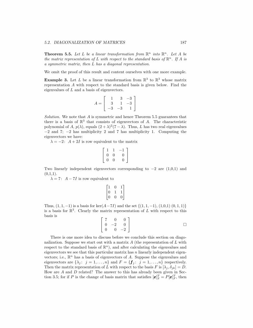
Theorem 5.5. Let L be a linear transformation from Rn into Rn. Let A bethe matrix representation of L with respect to the standard basis of Rn. If A isa symmetric matrix, then L has a diagonal representation.
We omit the proof of this result and content ourselves with one more example.
Example 3. Let L be a linear transformation from R3 to R3 whose matrixrepresentation A with respect to the standard basis is given below. Find theeigenvalues of L and a basis of eigenvectors.
A =
1 3 −33 1 −3
−3 −3 1
Solution. We note that A is symmetric and hence Theorem 5.5 guarantees thatthere is a basis of R3 that consists of eigenvectors of A. The characteristicpolynomial of A, p(λ), equals (2 + λ)2(7− λ). Thus, L has two real eigenvalues−2 and 7; −2 has multiplicity 2 and 7 has multiplicity 1. Computing theeigenvectors we have:
λ = −2: A+ 2I is row equivalent to the matrix
1 1 −10 0 00 0 0
Two linearly independent eigenvectors corresponding to −2 are (1,0,1) and(0,1,1).
λ = 7: A− 7I is row equivalent to
1 0 10 1 10 0 0
Thus, (1, 1,−1) is a basis for ker(A−7I) and the set {(1, 1,−1), (1,0,1) (0, 1, 1)}is a basis for R
3. Clearly the matrix representation of L with respect to thisbasis is
7 0 00 −2 00 0 −2
�
There is one more idea to discuss before we conclude this section on diago-nalization. Suppose we start out with a matrix A (the representation of L withrespect to the standard basis of Rn), and after calculating the eigenvalues andeigenvectors we see that this particular matrix has n linearly independent eigen-vectors; i.e., Rn has a basis of eigenvectors of A. Suppose the eigenvalues andeigenvectors are {λj : j = 1, . . . , n} and F = {fff j : j = 1, . . . , n} respectively.Then the matrix representation of L with respect to the basis F is [λj , δjk] = D.How are A and D related? The answer to this has already been given in Sec-tion 3.5; for if P is the change of basis matrix that satisfies [xxx]TS = P [xxx]TF , then

188 CHAPTER 5. EIGENVALUES AND EIGENVECTORS
P is easy to write out, for its columns are the coordinates of the eigenvectorswith respect to the standard basis. Moreover, we have
A = PDP−1 (5.5)
or
D = P−1AP
Note that in the formula D = P−1AP , the matrix that multiplies A on the rightis the matrix whose columns consist of the eigenvectors of A. Note also that Aand D are similar; cf. Section 3.5.
Example 4. Let A be the matrix
1 3 −33 1 −3
−3 −3 1
Since A is symmetric, we know that it can be diagonalized. In fact, in Example 3,we computed the eigenvalues and eigenvectors of A and got
λ1 = −2 fff1 = (1, 0, 1λ2 = −2 fff2 = (0, 1, 1)λ3 = 7 fff3 = (1, 1,−1)
Thus,
D =
−2 0 00 −2 00 0 7
and P =
1 0 10 1 11 1 −1
Computing P−1 we have
D = P−1AP
=1
3
2 −1 1−1 2 11 1 −1
1 3 −33 1 −3
−3 −3 1
1 0 10 1 11 1 −1
=
−2 0 00 −2 00 0 7
�
Formula (5.5) and the following calculations enable us to compute fairlyeasily the various powers of A, once we know the eigenvalues and eigenvectorsof this matrix.
A2 = [PDP−1][PDP−1] = PD(P−1P )DP−1 = PD2P−1
In a similar fashion, we have
An = PDnP−1 (5.6)
The advantage in using (5.6) to compute An is that D is a diagonal matrix andits powers are easy to calculate.
5.2. DIAGONALIZATION OF MATRICES 189
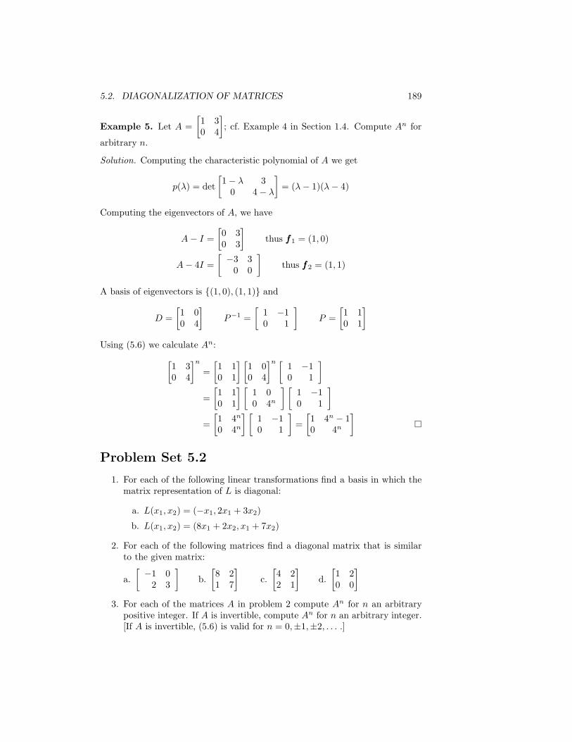
Example 5. Let A =
[
1 30 4
]
; cf. Example 4 in Section 1.4. Compute An for
arbitrary n.
Solution. Computing the characteristic polynomial of A we get
p(λ) = det
[
1− λ 30 4− λ
]
= (λ− 1)(λ− 4)
Computing the eigenvectors of A, we have
A− I =
[
0 30 3
]
thus fff1 = (1, 0)
A− 4I =
[
−3 30 0
]
thus fff2 = (1, 1)
A basis of eigenvectors is {(1, 0), (1, 1)} and
D =
[
1 00 4
]
P−1 =
[
1 −10 1
]
P =
[
1 10 1
]
Using (5.6) we calculate An:
[
1 30 4
]n
=
[
1 10 1
] [
1 00 4
]n [1 −10 1
]
=
[
1 10 1
] [
1 00 4n
] [
1 −10 1
]
=
[
1 4n
0 4n
] [
1 −10 1
]
=
[
1 4n − 10 4n
]
�
Problem Set 5.2
1. For each of the following linear transformations find a basis in which thematrix representation of L is diagonal:
a. L(x1, x2) = (−x1, 2x1 + 3x2)
b. L(x1, x2) = (8x1 + 2x2, x1 + 7x2)
2. For each of the following matrices find a diagonal matrix that is similarto the given matrix:
a.
[
−1 02 3
]
b.
[
8 21 7
]
c.
[
4 22 1
]
d.
[
1 20 0
]
3. For each of the matrices A in problem 2 compute An for n an arbitrarypositive integer. If A is invertible, compute An for n an arbitrary integer.[If A is invertible, (5.6) is valid for n = 0,±1,±2, . . . .]

190 CHAPTER 5. EIGENVALUES AND EIGENVECTORS
4. Let A be the matrix
A =
4 1 −11 4 −1
−1 −1 4
a. Find a matrix P such that P−1AP = D is a diagonal matrix.
b. Compute A10.
c. Compute A−10.
5. Let A be the matrix
A =
3 0 1 −22 3 2 −40 0 2 01 0 1 0
a. Compute the eigenvalues and eigenvectors of A.
b. Find a matrix P such that P−1AP is a diagonal matrix.
c. Compute A3.
6. Let L : V → W be a linear transformation. Suppose dim(V ) = n anddim(W ) = m. Show that it is possible to pick bases in V and W suchthat the matrix representation of L with respect to these bases is an m×nmatrix A = [ajk] with ajk = 0 if j is not equal to k and akk equals zeroor one. Moreover, the number of ones that occur in A is exactly equal todim(Rg(L)) = rank(A).
7. Let Ap = [apjk] be a sequence of n× n matrices. We say that limp→∞
Ap =
A = [ajk], if and only if limp→∞
apjk = ajk for each j and k. For each of the
matrices in problem 2, determine whether or not limn→∞
An exists, and then
evaluate the limit if possible.
8. For the matrix A in problem 5, limn→∞
An =?
9. Let A =
[
λ1 00 λ2
]
. Let g(λ) =∑p
k=0 gkλk be any polynomial in λ. Define
g(A) by g(A) =∑p
k=0 gkAk. Show that
g(A) =
[
g(λ1) 00 g(λ2)
]
Generalize this formula to the case when A is an n× n diagonal matrix.
10. Suppose A and B are similar matrices. Thus, A = PBP−1 for somenonsingular matrix P . Let g(λ) be any polynomial in λ. Show thatg(A) = Pg(B)P−1.
5.3. APPLICATIONS 191
11. If c is a nonnegative real number, we can compute its square root. In factcα is defined for any real number α if c > 0. Suppose A is a diagonalizablematrix with nonnegative eigenvalues. Thus A = PDP−1, where D equals[λjδjk]. Define Aα = PDαP−1, where Dα = [λαj δjk].
a. Show that (D1/2)2 = D, assuming λj ≥ 0.
b. Show that (A1/2)2 = A, with the same assumption as in a.
12. For each matrix A below compute A1/2.
a.
[
8 11 7
]
b.
[
4 22 1
]
c.
4 1 −11 4 −1
−1 −1 4
13. For each matrix in the preceding problem compute when possible A−1/6
and A2/3.
14. Compute A1/2 and A−1/2 where A is the matrix in problem 5. Verify thatA1/2A−1/2 = I.
5.3 Applications
In this section, instead of presenting any new material we discuss and analyzea few problems by employing the techniques of the preceding sections. Severalthings should be observed. One is the recasting of the problem into the lan-guage of matrices, and the other is the method of analyzing matrices via theireigenvalues and eigenvectors.
The reader should also be aware that these problems are contrived, in thesense that they do not model (to the author’s knowledge) any real phenomenon.They were made up so that the arithmetic would not be too tedious and yet theflavor of certain types of analyses would be allowed to seep through. Modelingreal world problems mathematically usually leads to a lengthy analysis of thephysical situation. This is done so that the mathematical model is believable;that is, we wish to analyze a mathematical structure, for us a matrix, and thenbe able, from this analysis, to infer something about the original problem. Inmost cases this just takes too much time—not the analysis, but making themodel believable.
Example 1. An individual has some money that is to be invested in threedifferent accounts. The first, second, and third investments realize a profit of 8,10, and 12 percent per year, respectively. Suppose our investor decides that atthe end of each year, one-fourth of the money earned in the second investmentand three-fourths of that earned in the third investment should be transferredinto the first account, and that one-fourth of the third account’s earnings willbe transferred to the second account. Assuming that each account starts outwith the same amount, how long will it take for the money in the first accountto double?
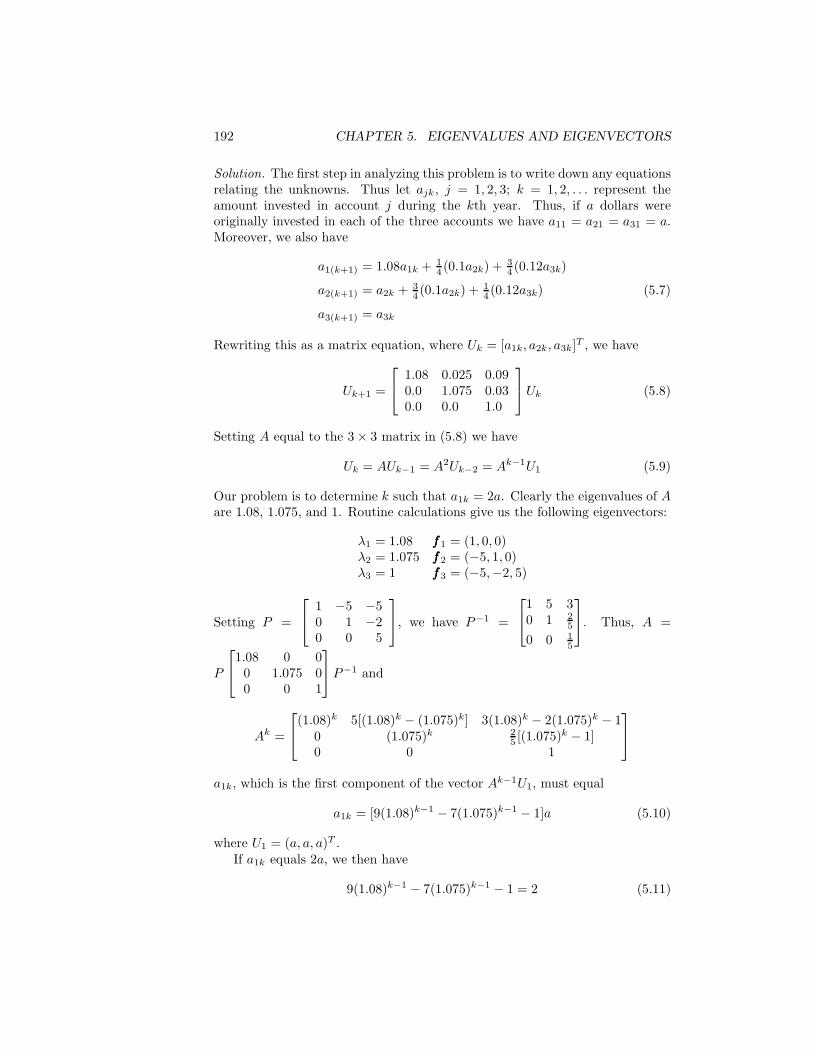
192 CHAPTER 5. EIGENVALUES AND EIGENVECTORS
Solution. The first step in analyzing this problem is to write down any equationsrelating the unknowns. Thus let ajk, j = 1, 2, 3; k = 1, 2, . . . represent theamount invested in account j during the kth year. Thus, if a dollars wereoriginally invested in each of the three accounts we have a11 = a21 = a31 = a.Moreover, we also have
a1(k+1) = 1.08a1k +14 (0.1a2k) +
34 (0.12a3k)
a2(k+1) = a2k +34 (0.1a2k) +
14 (0.12a3k)
a3(k+1) = a3k
(5.7)
Rewriting this as a matrix equation, where Uk = [a1k, a2k, a3k]T , we have
Uk+1 =
1.08 0.025 0.090.0 1.075 0.030.0 0.0 1.0
Uk (5.8)
Setting A equal to the 3× 3 matrix in (5.8) we have
Uk = AUk−1 = A2Uk−2 = Ak−1U1 (5.9)
Our problem is to determine k such that a1k = 2a. Clearly the eigenvalues of Aare 1.08, 1.075, and 1. Routine calculations give us the following eigenvectors:
λ1 = 1.08 fff1 = (1, 0, 0)λ2 = 1.075 fff2 = (−5, 1, 0)λ3 = 1 fff3 = (−5,−2, 5)
Setting P =
1 −5 −50 1 −20 0 5
, we have P−1 =
1 5 30 1 2
5
0 0 15
. Thus, A =
P
1.08 0 00 1.075 00 0 1
P−1 and
Ak =
(1.08)k 5[(1.08)k − (1.075)k] 3(1.08)k − 2(1.075)k − 10 (1.075)k 2
5 [(1.075)k − 1]
0 0 1
a1k, which is the first component of the vector Ak−1U1, must equal
a1k = [9(1.08)k−1 − 7(1.075)k−1 − 1]a (5.10)
where U1 = (a, a, a)T .If a1k equals 2a, we then have
9(1.08)k−1 − 7(1.075)k−1 − 1 = 2 (5.11)
5.3. APPLICATIONS 193
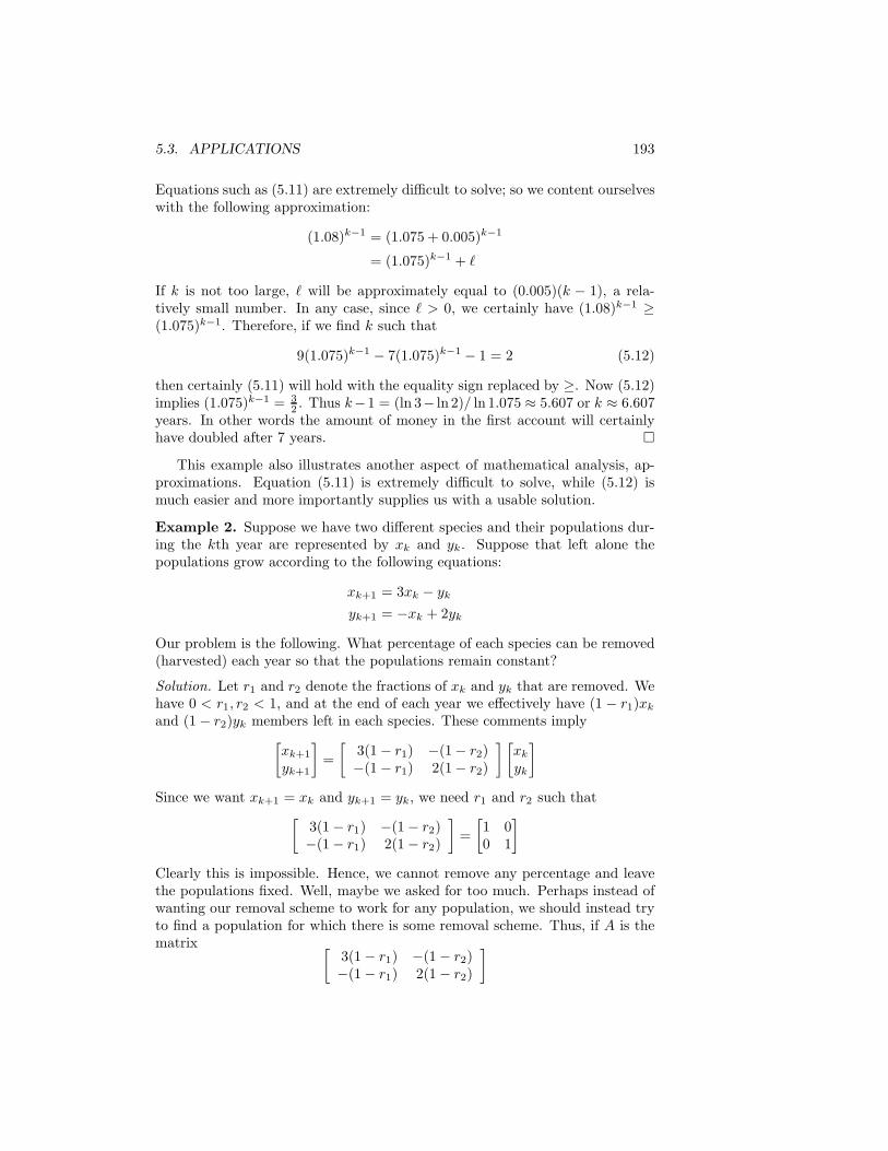
Equations such as (5.11) are extremely difficult to solve; so we content ourselveswith the following approximation:
(1.08)k−1 = (1.075 + 0.005)k−1
= (1.075)k−1 + ℓ
If k is not too large, ℓ will be approximately equal to (0.005)(k − 1), a rela-tively small number. In any case, since ℓ > 0, we certainly have (1.08)k−1 ≥(1.075)k−1. Therefore, if we find k such that
9(1.075)k−1 − 7(1.075)k−1 − 1 = 2 (5.12)
then certainly (5.11) will hold with the equality sign replaced by ≥. Now (5.12)implies (1.075)k−1 = 3
2 . Thus k−1 = (ln 3− ln 2)/ ln 1.075 ≈ 5.607 or k ≈ 6.607years. In other words the amount of money in the first account will certainlyhave doubled after 7 years. �
This example also illustrates another aspect of mathematical analysis, ap-proximations. Equation (5.11) is extremely difficult to solve, while (5.12) ismuch easier and more importantly supplies us with a usable solution.
Example 2. Suppose we have two different species and their populations dur-ing the kth year are represented by xk and yk. Suppose that left alone thepopulations grow according to the following equations:
xk+1 = 3xk − yk
yk+1 = −xk + 2yk
Our problem is the following. What percentage of each species can be removed(harvested) each year so that the populations remain constant?
Solution. Let r1 and r2 denote the fractions of xk and yk that are removed. Wehave 0 < r1, r2 < 1, and at the end of each year we effectively have (1 − r1)xkand (1− r2)yk members left in each species. These comments imply
[
xk+1
yk+1
]
=
[
3(1− r1) −(1− r2)−(1− r1) 2(1− r2)
] [
xkyk
]
Since we want xk+1 = xk and yk+1 = yk, we need r1 and r2 such that[
3(1− r1) −(1− r2)−(1− r1) 2(1− r2)
]
=
[
1 00 1
]
Clearly this is impossible. Hence, we cannot remove any percentage and leavethe populations fixed. Well, maybe we asked for too much. Perhaps instead ofwanting our removal scheme to work for any population, we should instead tryto find a population for which there is some removal scheme. Thus, if A is thematrix
[
3(1− r1) −(1− r2)−(1− r1) 2(1− r2)
]

194 CHAPTER 5. EIGENVALUES AND EIGENVECTORS
we want to find numbers x and y such that A[
x y]T
=[
x y]T
. In otherwords, can we pick r1 and r2 so that 1 not only is an eigenvalue for A but alsohas an eigenvector with positive components. Let’s compute the characteristicpolynomial of A.
p(λ; r1, r2) = det
[
3(1− r1)− λ −(1− r2)−(1− r1) 2(1− r2)− λ
]
= [λ− 3(1− r1)][λ− 2(1− r2)]− (1− r1)(1− r2)
= λ2 − (5− 3r1 − 2r2)λ+ 5(1− r1)(1− r2)
Now we want p(1; r1, r2) = 0. Setting λ = 1, we have after some simplification
r1(5r2 − 2) = 3r2 − 1 (5.13)
where we want rk, k = 1 or 2, to lie between 0 and 1. Solving (5.13) for r1 andchecking the various possibilities to ensure that both rk’s lie between 0 and 1,we have
r1 =3r2 − 1
5r2 − 20 < r2 <
1
3or
1
2< r2 < 1 (5.14)
For r1 and r2 so related let’s calculate the eigenvectors of the eigenvalue 1. Thematrix
A− I2 =
[
2− 3r1 −(1− r2)−(1− r1) 1− 2r2
]
is row equivalent to the matrix
1
5r2 − 21
0 0
Thus, the eigenvector (x, y) corresponding to λ = 1 satisfies x = (2 − 5r2)y. Ifboth x and y are to be positive we clearly need 2 − 5r2 positive. We thereforehave the following solution to our original problem. First r1 = (3r2−1)/(5r2−2),where r2 satisfies the inequalities in (5.14). To ensure that x and y are positivewe then restrict r2 to satisfy 0 < r2 <
13 only. In conclusion, if we harvest less
than 13 of the second species and (3r2 − 1)/(5r2 − 2) of the first species where
the two species are in the ratio 1/(2− 5r2), we will have a constant populationfrom one year to the next. �
Example 3. This last example is interesting in that it is not all clear how toexpress the problem in terms of matrices. Suppose we construct the followingsequence of numbers: let a0 = 0 and a1 = 1, a2 = 1
2 , a3 = (1 + 12 )/2 = 3
4 ,a4 = (12 + 3
4 )/2 = 58 , and in general an+2 = (an + an+1)/2; that is, an+2 is
the average of the two preceding numbers. Do these numbers approach someconstant as n gets larger and larger?

5.3. APPLICATIONS 195
Solution. Let Un =[
an−1 an]T
for n = 1, 2, . . . . Recalling how the an aredefined, we have
Un+1 =
[
anan+1
]
=
an
an+1
2+an2
=
0 1
1
2
1
2
[
an−1
an
]
= AUn (5.15)
where A is the 2 × 2 matrix appearing in (5.15). As in similar examples, we
have Un = An−1U1, where U1 equals[
0 1]T
. The characteristic polynomial ofA is
p(λ) = det(A− λI) = det
−λ 1
1
2
1
2− λ
=1
2(2λ+ 1)(λ− 1)
Thus, the eigenvalues of A are 1 and − 12 . We will see later that, if the an have
a limiting value, it is necessary for the number 1 to be an eigenvalue.
λ1 = 1, fff1 = (1, 1)
λ = −1
2, fff2 = (−2, 1)
Setting P equal to
[
1 −21 1
]
, we calculate P−1 = 13
[
1 2−1 1
]
. Thus, we
have
An =
[
1 −21 1
]
1 0
0
(
−1
2
)n
1
3
2
3
−1
3
1
3
Clearly, the larger n gets the closer the middle matrix on the right-hand side
gets to the matrix
[
1 00 0
]
which means that the vector Un = An−1U1 gets close
to the vector U∞, where
U∞ =
[
1 −21 1
] [
1 00 0
]
1
3
2
3
−1
3
1
3
[
01
]
=
1
3
2
31
3
2
3
[
01
]
=
2
32
3
Thus, Un =[
an−1 an]T
gets close to[
23
23
]T, which means that the numbers
an get close to the number 23 . Notice too that U∞ is an eigenvector of A
196 CHAPTER 5. EIGENVALUES AND EIGENVECTORS
corresponding to the eigenvalue 1. In fact, this was to be expected from theequation Un+1 = AUn; for if the Un converge to something nonzero, calledU∞, then U∞ must satisfy the equation U∞ = AU∞. That is, U∞ must be aneigenvector of the matrix A corresponding to the eigenvalue 1. This is why 1must be an eigenvalue. �
Problem Set 5.3
1. Suppose we have a single species that increases from one year to the nextaccording to the rule
xk+1 = 2xk
What percentage of the population can be harvested and have the popu-lation remain constant from one year to the next? If the initial populationequals 10, assuming no harvesting, what will the population be in 20 years?
2. The following sequence of numbers is called the Fibonacci sequence:
a0 = 1, a1 = 1, a2 = 2, a3 = 3, . . . , an+1 = an + an−1
Find a general formula for an and determine its limit if one exists.
3. Define the following sequence of numbers:
a0 = a a1 = b a2 =1
3a0 +
2
3a1 and an+2 =
1
3an +
2
3an+1
Find a general formula for an and determine its limiting behavior.
4. Define the following sequence of numbers:
a0 = a a1 = b a2 = ca0 + da1 an+2 = can + dan+1
a. If c and d are nonnegative and c+ d = 1, determine a formula for anand the limiting behavior of this sequence.
b. What happens if we just assume that c+ d = 1?
c. What happens if there are no restrictions on c and d?
5. Suppose there are two cities, the sum of whose populations remains con-stant. Assume that each year a certain fraction of one city’s populationmoves to the second city and the same fraction of the second city’s popu-lation moves to the first city. Let xk and yk denote each city’s populationin the kth year.
a. Find formulas for xk+1 and yk+1 in terms of xk and yk. These for-mulas will of course depend on the fraction r of the populations thatmove.
b. What is the limiting population of each city in terms of the originalpopulations and r?
5.3. APPLICATIONS 197
6. We again have the same two cities as in problem 5, only this time let’sassume that r1 represents the fraction of the first city’s population thatmoves to the second city and r2 the fraction of the second city’s populationthat moves to the first city.
a. Find formulas for xk+1 and yk+1.
b. What is the limiting population of each city?
7. Suppose that the populations of two species change from one year to thenext according to the equations
xk+1 = 4xk + 3yk
yk+1 = 3xk + 9yk
Are there any initial populations and harvesting schemes that leave thepopulations constant from one year to the next?
8. Let u0 = a > 0, u1 = b > 0. Define u2 = u0u1, un+2 = unun+1. What islim un? Hint: log un =?
Supplementary Problems
1. Define and give examples of the following:
a. Eigenvector and eigenvalue
b. Eigenspace
c. Characteristic matrix and polynomial
2. Find a linear transformation from R3 to R3 such that 4 is an eigenvalueof multiplicity 2 and 5 is an eigenvalue of multiplicity 1.
3. Let L be a linear transformation from V to V . Let λ be any eigenvalue ofL, and let Kλ be the eigenspace of λ. That is, Kλ = {xxx : Lxxx = λxxx}. Showthat Kλ is a subspace of V , and that it is invariant under L, cf. number13 in the Supplementary Problems for Chapter 3.
4. Let λ be an eigenvector of L. A nonzero vector xxx is said to be a generalizedeigenvector of L, if there is a positive integer k such that
[L− λI]kxxx = 000
Show that the set of all generalized eigenvectors of λ along with the zerovector is an invariant subspace.
5. Let
A =
2 1 00 2 10 0 2

198 CHAPTER 5. EIGENVALUES AND EIGENVECTORS
a. Find all the eigenvalues of A.
b. Find the eigenspaces of A.
c. Find the generalized eigenspaces of A; cf. problem 4.
6. Let
A =
1 2 −40 −1 60 −1 4
a. Determine the eigenvalues and eigenspaces of A.
b. Show that A is not similar to a diagonal matrix.
c. Find the generalized eigenspaces of A.
7. Let L be a linear transformation from R2 to R2. Let xxx be a vector in R2
for which xxx and Lxxx are not zero, but for which L2xxx = 000.
a. Show that F = {Lxxx,xxx} is linearly independent.
b. Show that the matrix representation A of L with respect to the basis
F of part a equals
[
0 10 0
]
.
c. Deduce that L2yyy = 0 for every vector yyy in R2.
8. Suppose that L is a linear transformation from R3 to R
3, and there is avector xxx for which L2xxx = 000, but xxx, Lxxx, and L2xxx are not equal to the zerovector. Set F = {L2xxx, Lxxx,xxx}.
a. Show that F is a basis of R3.
b. Find the matrix representation A of L with respect to the basis F .
c. Show that L3yyy = 000 for every vector yyy in R3.
9. Let
A =
1 0 0 20 1 3 00 0 2 00 0 0 2
Find a matrix P such that P−1AP is a diagonal matrix. Compute A10.
10. A mapping T from a vector space V into V is called affine if Txxx = Lxxx+aaa,where L is a linear transformation and a is a fixed vector in V .
a. Show that T nxxx = Lnxxx +∑n−1
k=0 Lkaaa. Thus every power of T is also
an affine transformation.
b. Let A =
[
2 33 2
]
. Define Txxx = Axxx+
[
13
]
. If xxx = (1, 1), compute T 10xxx.
Hint: 1 + r + · · ·+ rn = [1− rn+1][1− r]−1.
5.3. APPLICATIONS 199
11. Let V = {∑2n=0 an cosnt : an any real number}.
a. Show that {1, cos t, cos 2t} is a basis of V .
b. Define L : V → V by L(∑2
n=0 an cosnt) =∑2
n=0 −n2an cosnt. Findthe eigenvalues and eigenvectors of L. Note that L[f ] = −f ′′.
c. Find L1/2, i.e., find a linear transformation T such that T 2 = L.
d. For any positive integers p and q find Lp/q.
12. Consider the following set of directions. Start at the origin, facing towardthe positive x1 axis, turn 45 degrees counterclockwise, and walk 1 unit inthis direction. Thus, you will be at the point (1/
√2, 1/
√2). Then turn 45
degrees counterclockwise and walk 12 unit in this new direction; then turn
45 degrees counterclockwise and walk 14 unit in this direction. If a cycle
consists of a 45-degree counterclockwise rotation plus a walk that is halfas long as the previous walk, where will you be after 20 cycles?
13. Let M be the set of 2× 2 matrices A for which
A
[
10
]
= λ
[
10
]
for some real number λ. That is, A is in M if (1,0) is an eigenvector of A.
a. Show that M is a subspace of M22.
b. Find a basis for M .
14. Let xxx be a fixed nonzero vector in Rn. Let Mxxx be the set of n×n matricesfor which xxx is an eigenvector.
a. Show that Mxxx is a subspace of Mnn.
b. If xxx = eee1, find a basis for Mxxx.
c. Can you find a basis for Mxxx if xxx is arbitrary? Hint: If B is aninvertible n× n matrix for which Bxxx1 = xxx2, then BAB
−1 is in Mxxx2
if A is in Mxxx1 .

200 CHAPTER 5. EIGENVALUES AND EIGENVECTORS