Efﬁcient Gradient-Domain Compositing Using an Approximate...

Pacific Graphics 2017J. Barbic and O. Sorkine-Hornung(Guest Editors)

Volume 36 (2017), Number 7

Efficient Gradient-Domain Compositing Using an Approximate

Curl-free Wavelet Projection

Xiaohua Ren1 , Luan Lyu1, Xiaowei He2, Yanci Zhang†3 and Enhua Wu‡1,2,4

1University of Macau, 2State Key Lab. of CS, ISCAS & Univ. of CAS, 3 Sichuan University,4Zhuhai-UM Science and Technology Research Institute

Figure 1: Red rock: A 19588×4457 (83-megapixel) panorama (top row) from 9 photos produced by our curl-free wavelet projection in 26.11s

on CPU and 0.45s on GPU. The bottom row is the extracted wavelet coefficients by our method. (Data is courtesy of Aseem Agarwala.)

Abstract

Gradient-domain compositing has been widely used to create a seamless composite with gradient close to a composite gradient

field generated from one or more registered images. The key to this problem is to solve a Poisson equation, whose unknown

variables can reach the size of the composite if no region of interest is drawn explicitly, thus making both the time and memory

cost expensive in processing multi-megapixel images. In this paper, we propose an approximate projection method based on

biorthogonal Multiresolution Analyses (MRA) to solve the Poisson equation. Unlike previous Poisson equation solvers which

try to converge to the accurate solution with iterative algorithms, we use biorthogonal compactly supported curl-free wavelets as

the fundamental bases to approximately project the composite gradient field onto a curl-free vector space. Then, the composite

can be efficiently recovered by applying a fast inverse wavelet transform. Considering an n-pixel composite, our method only

requires 2n of memory for all vector fields and is more efficient than state-of-the-art methods while achieving almost identical

results. Specifically, experiments show that our method gains a 5x speedup over the streaming multigrid in certain cases.

Categories and Subject Descriptors (according to ACM CCS): I.3.3 [Computer Graphics]: Picture/Image Generation—Displayalgorithms

1. Introduction

Gradient-domain compositing is one of the most important tech-niques in image processing, which has been widely used in appli-cations such as seamless cloning [PGB03,JSTS06,FHL∗09], seam-less stitching [Aga07,YHLX13,LDLM15], gradient domain paint-ing [MP08]. Its basic idea is to find a composite image whose gra-dients best match a composite gradient field extracted from two ormore registered images. This matching process is actually equiva-lent to solving a Poisson equation. Although there exist a lot of al-

† [email protected]‡ [email protected]

gorithms that can be used to efficiently solve the Poisson equation,gradient-domain compositing for large images still remains a chal-lenge. One reason is that direct solvers like Cholesky factorizationand Gaussian elimination become impractical for large linear sys-tem of equations. Iterative solvers like conjugate gradients are ap-plicable to large sparse systems, but would require many iterationsto get the desired solution if no preconditioning technique, which isusually non-parallelizable, is used. Another reason is that efficien-t iterative solvers like traditional multgrid consume 8/3n memoryfor two dimensions. As the number of pixels increases, solving thelinear system entirely in-core quickly becomes impossible.

According to Helmholtz-Hodge decomposition, any sufficientlysmooth vector field can be decomposed into the sum of a curl-free

c© 2017 The Author(s)Computer Graphics Forum c© 2017 The Eurographics Association and JohnWiley & Sons Ltd. Published by John Wiley & Sons Ltd.

Ren et al. / Efficient Gradient-Domain Compositing Using an Approximate Curl-free Wavelet Projection

vector field and a divergence-free vector field for a simply con-nected domain (like an image). Therefore, we can reformulate thePoisson equation as a projection problem which projects the com-posite gradient field onto a curl-free vector space. The key now be-comes how can we find an appropriate curl-free basis for the curl-free space so that the projection is both lightweight and efficient.As we know, the most commonly used curl-free basis is the orthog-onal basis based on cosine functions, which can lead to an accu-rate Poisson-equation solution. Unfortunately, cosine functions areglobal, and the complexity is O(nlogn). Its total computation costcan be twice that of the modern iterative methods according to [M-cC08, BCCZ08].

Considering the Poisson-equation solution will be rounded offto integer numbers ranging from 0 to 255 in image applications, itis actually not necessary to get a solution with high accuracy. Thismotivates us to propose an approximate projection method to solvethe Poisson equation. Inspired by works in fluid dynamics [Ur-b00, DP06], we use spline functions to form compactly support-ed biorthogonal curl-free bases for the projection. Then, we showthat the projection can be highly parallelized on GPU with onlya small extra memory cost by applying the lifting wavelet trans-form [SS96]. Compared to an exact projection based on orthogo-nal bases, our approximate projection based on biorthogonal curl-free bases is sufficient to get almost identical results for gradient-domain compositing with the following advantages

• Our approximate projection has an O(n) time-complexity, whichonly consists of three fast wavelet transforms.

• By applying the lifting wavelet transform, our method only needs2n of memory for an n-pixel composite, making it possible toprocess larger in-core images.

• Our method is highly parallelizable, which can be fully exploitedon modern GPUs to achieve an order of magnitude speedup overthe CPU implementation.

2. Related Work

The Poisson equation arises from many areas and a lot of practi-cal algorithms are available to solve this problem. Direct methodssuch as Cholesky decomposition and Gaussian elimination are veryaccurate at solving small-scale problems. However, for large-scaleproblems, iterative methods are better choice, in items of compu-tation time and memory storage (e.g., direct methods would needextra storage for the factored matrix). Simple iterative methods likeJacobi and Gauss-Seidel are efficient for each iteration, but theyrequire many iterations to remove low-frequency errors. Jeschkeet al. [JCW09] point out that the convergence rate of the Jacobimethod can be accelerated by appropriately choosing the right s-tencil size. Alternatively, the number of iterations can be greatlyreduced by applying a multigrid scheme [BHM00], which has anO(n) time cost and 8/3n memory cost for 2D cases. The multigridmethod has also been widely used in gradient-domain composit-ing, such as high dynamic range compression [FLW02] and real-time painting [MP08]. Unfortunately, traditional multigrid method-s require multiple V-cycles, which are inefficient for solving largelinear systems with out-of-core data. Kazhdan and Hoppe [KH08]address this problem by proposing a streaming multigrid solver,which needs just two sequential passes over out-of-core data. Their

method is later extended to handle spherical images in [KH10]and to run on a distributed computer cluster with multiple nodesin [KSH10].

Besides the multigrid methods, conjugate gradient methods al-so converge much faster than the Jacobi or Gauss-Seidel method-s, especially when a preconditioner is also used. Pérez et al. [PG-B03] use the preconditioned conjugate gradient method for seam-less cloning and Agarwala et al. [ADA∗04] for gradient-domaincompositing. Later, Agarwala [Aga07] solves a reduced linear sys-tem by exploiting the fact the difference between a simple colorcomposite and its associated gradient-domain composite is largelysmooth. Szeliski et al. [SUS11] propose a similar technique usinglow-dimensional B-splines to represent the offset field. Similarly,Farbman et al. [FHL∗09] use mean value coordinates (MVC) de-fined over an adaptive triangulation of the cloned region to interpo-late the offset field at the region boundary or the seams. To accel-erate the convergence rate, Szeliski [Sze90] proposes to use hierar-chical basis functions as the preconditioner, which is later improvedin [Sze06]. Although these two methods are efficient at solving thePoisson equation, they typically require more memory usage as dis-cussed in [Aga07]. Besides, parallelizing the preconditioning stepis usually not an easy task (e.g., preconditioning via Gauss-Seidelsteps requires advanced techniques).

Over the last decades, wavelets have been widely used in im-age processing, such as denoising, compression, fusion, etc. Butthere are very few works that apply wavelets to improve the effi-ciency of gradient-domain compositing. Burt and Adelson [BA83]first propose to use multiresolution B-splines to hide the seam-s at different scales. Urban [Urb00] constructs curl-free wavelet-s to supplement the divergence-free wavelets [LR92]. With boththe curl-free and divergence-free wavelets, Deriaz and Perrier [D-P06] propose a novel iterative algorithm to decompose a gener-al vector field into the sum of a curl-free part and a divergence-free part by alternatively performing curl-free and divergence-freeprojections. The problem with their work is that it is only appli-cable to problems with periodic boundary conditions. Manson etal. [MPS08] propose a wavelet method to reconstruct the indica-tor function of a solid from an oriented point cloud. Farbmann etal. [FFL11] introduced a pyramidal convolution approach to solvelinear translation-invariant problems with O(n) time cost and 8/3n

memory cost. Recently, Edge-avoiding wavelets are constructed us-ing the lifting scheme in [Fat09] to avoid the difficulties in solv-ing large and poorly-conditioned systems of equations. Later, thismethod is extended by applying the À-Trous wavelet transform [D-SHL10, HDL11]. Compared to the lifting wavelet transform, theÀ-Trous wavelet transform has s ·n extra memory cost with s beingthe number of scales to transform. Note that edge-voiding waveletsare designed to process scalar fields, we focus on handling vectorfields.

3. Background

In this section, we first review the problem of gradient-domaincompositing and its solution techniques. Then, we present a solverbased on curl-free cosine functions. Finally, we briefly discuss it-s disadvantages, which motivate us to use more general curl-freebases to overcome them.

c© 2017 The Author(s)Computer Graphics Forum c© 2017 The Eurographics Association and John Wiley & Sons Ltd.


Notation. Scalars appear in lower case: x and vectors inbold lower case: x. 〈u,v〉 and uv denote inner product and thecomponent-wise multiplication of u and v, respectively. A vectorfield whose curl is zero is called a curl-free field, which can be rep-resented as the gradient of a scalar field p, i.e. uc =∇p. We denoteL2(Ω) the vector space of all scalar functions f (x) : Ω → R of fi-nite energy and L2(Ω) := L2 ×L2 the vector space of all vector

fields over Ω. Both spaces are equipped with the Euclidean nor-m. The curl-free space denoted by H0

c(Ω) is the subspace formedby all the curl-free fields in L2(Ω). R, N and Z are used to de-note the set of all real numbers, natural numbers and integers, re-spectively. A 2 j-scaled and k-shifted function of f (x) is written asf j,k := f (2 jx− k) for j,k ∈ Z.

3.1. Gradient-domain compositing

In gradient-domain compositing, a composite vector field u ∈L2(Ω) is generated by copying and blending the gradients of oneor more registered images, which may not be a curl-free or conser-vative field. Our purpose is to find uc ∈ H0

c(Ω) that is closest to u

by solving the minimization problem:

minuc∈H0

c(Ω)

12

∫Ω‖u−uc‖2. (1)

One solution of the problem is to solving a Poisson equation. Sub-stituting uc =∇p and using the Euler-Lagrange equation yield

∆p =∇·u (2)

After discretizing the Poisson equation, direct or iterative solverscan be used to solve it.

Another solution is by projecting u onto H0c(Ω), if orthogonal

bases of H0c(Ω) are given. As an example, we use the well-known

curl-free cosine functions to illustrate the basic idea.

3.2. A solver using curl-free cosine functions

Curl-free cosine functions. It’s known that the set of cosine func-tions ϕk = cos(k1x)cos(k2y) is an orthogonal basis of L2(Ω =[0,π]2) with Neumann BCs, where k = [k1,k2]

T ∈ N2. Then, the

curl-free cosine functions are defined as

Φc,k =∇ϕk =−kΦk, (3)

where

Φk =

[

sin(k1x)cos(k2y)cos(k1x)sin(k2y)

]

. (4)

Finally, we have Φc,k and Φk, which are orthogonal bases of

H0c(Ω) and L2(Ω), respectively.

Curl-free cosine projection. With these bases, we take threesteps to obtain the closest uc of u as well as the scalar field p. First,the coefficients u = [ux, uy]

T of u = ∑k u(k)Φk are computed byapplying the sine and cosine transforms of u. Then, the coefficientsuc of uc = ∑k uc(k)Φc,k are computed by projecting u(k) onto k:

uc(k) =−〈k, u(k)〉‖k‖2 . (5)

Please refer to Appendix A for a derivation of the above equation.Finally, uc and p are reconstructed by

p = ∑k

uc(k)ϕk, uc =∇p. (6)

Discussion. Because curl-free cosine functions are orthogonal,the solution is exact. However, since sine/cosine functions are glob-al, the cosine/sine transform is time-consuming, whose best timecomplexity is O(nlogn) in case that the size of signal is power-of-two. In this paper, we explore to use biorthogonal compactly sup-

ported curl-free wavelets, whose transforms have O(n) time com-plexity.

4. Our Solver using Curl-free Wavelets

Multiresolution analysis (MRA). A MRA of L2(R) is a se-quence of closed subspaces V j = spanϕ j,kk∈Z j∈Z satisfyingV j ⊂ V j+1 and some other properties defined in [Mal08], whereϕ(x) is referred to as a scaling function of the MRA. Wavelet s-paces W j = spanψ j,kk∈Z are the complements such that V j+1 =V j ⊕W j, where ⊕ indicates the direct sum. ψ(x) is referred to asa wavelet of the MRA. Then we have the wavelet space decompo-sition L2(R) = V0 ⊕ j∈N W j . For simplicity we write ϕ0,k,ψ j,kto denote the basis of L2(R) generated by a MRA with associatedscaling function and wavelet (ϕ,ψ).

By tensor-products of L2(R) = V0 ⊕ j∈N W j, the wavelet s-

pace decomposition of the 2D function space is L2(R2) = V0 ⊕j1

Wj1⊕j2

Wj2⊕j3 Wj3 , where 0=(0,0), j1 =( j1,0), j2 =(0, j2), j3 =

( j1, j2) and j1, j2 ∈N. The base functions of V0 = spanϕ0,k andWje

= spanψje,k for e ∈ 1,2,3 are defined by tensor-productsof ϕ j,k,ψ j,k:

ϕ0,k = ϕ0,k1 ϕ0,k2 ,ψj1,k = ψ j1,k1 ϕ0,k2 ,

ψj2,k = ϕ0,k1 ψ j2,k2 ,ψj3,k = ψ j1,k1 ψ j2,k2 .(7)

Similarly, we write ϕ0,k,ψje,k to denote the basis of L2(R2)formed by above base functions.

Notice that curl-free cosine functions are actually the gradientsof cosine functions. In one dimension, the derivative of cos(kx)is −k sin(kx) and either of them forms a basis of L2([0,π]) withcorresponding BCs. So in order to construct more general curl-freewavelet bases, a crucial step is to find two bases linked by differen-tiation like cosine and sine functions. The existence of such pairs ofbases is guaranteed by Lemarié-Rieusset’s proposition in [LR92].The following English version is borrowed from [DP09].

Proposition: Let V 1j be a MRA of L2(R), with associated

scaling function and wavelet (ϕ1,ψ1). Then, there exists a M-RA V 0

j of L2(R), with associated scaling function and wavelet

(ϕ0,ψ0), satisfying:

(ϕ1)′

(x) = ϕ0(x)−ϕ0(x−1), (8a)

(ψ1)′

(x) = 4 ·ψ0(x). (8b)

Famous pairs of (ϕ1,ψ1) and (ϕ0,ψ0) satisfying Equations (8a, 8b)are B-splines of degree n and n− 1, with corresponding waveletsof vanishing moment m and m + 1. These scaling functions and



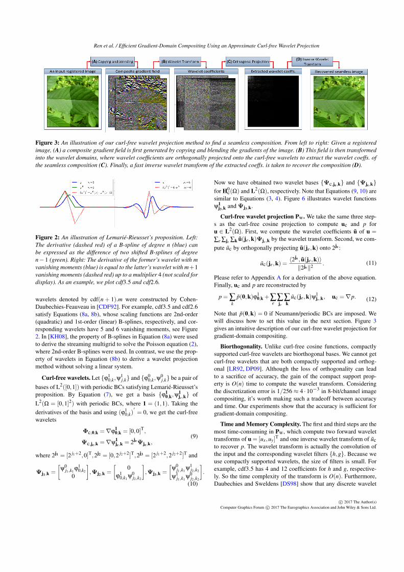
Figure 3: An illustration of our curl-free wavelet projection method to find a seamless composition. From left to right: Given a registered

image, (A) a composite gradient field is first generated by copying and blending the gradients of the image. (B) This field is then transformed

into the wavelet domains, where wavelet coefficients are orthogonally projected onto the curl-free wavelets to extract the wavelet coeffs. of

the seamless composition (C). Finally, a fast inverse wavelet transform of the extracted coeffs. is taken to recover the composition (D).

Figure 2: An illustration of Lemarié-Rieusset’s proposition. Left:

The derivative (dashed red) of a B-spline of degree n (blue) can

be expressed as the difference of two shifted B-splines of degree

n−1 (green). Right: The derivative of the former’s wavelet with m

vanishing moments (blue) is equal to the latter’s wavelet with m+1vanishing moments (dashed red) up to a multiplier 4 (not scaled for

display). As an example, we plot cdf3.5 and cdf2.6.

wavelets denoted by cdf(n + 1).m were constructed by Cohen-Daubechies-Feauveau in [CDF92]. For example, cdf3.5 and cdf2.6satisfy Equations (8a, 8b), whose scaling functions are 2nd-order(quadratic) and 1st-order (linear) B-splines, respectively, and cor-responding wavelets have 5 and 6 vanishing moments, see Figure2. In [KH08], the property of B-splines in Equation (8a) were usedto derive the streaming multigrid to solve the Poisson equation (2),where 2nd-order B-splines were used. In contrast, we use the prop-erty of wavelets in Equation (8b) to derive a wavelet projectionmethod without solving a linear system.

Curl-free wavelets. Let ϕ10,k,ψ

1j,k and ϕ0

0,k,ψ0j,k be a pair of

bases of L2([0,1]) with periodic BCs satisfying Lemarié-Rieusset’sproposition. By Equation (7), we get a basis ϕ1

0,k,ψ1je,k of

L2(Ω = [0,1]2) with periodic BCs, where 1 = (1,1). Taking the

derivatives of the basis and using (ϕ10,k)

′

= 0, we get the curl-freewavelets

Φc,0,k =∇ϕ10,k = [0,0]T,

Ψc,je,k =∇ψ1je,k = 2je

Ψje,k,(9)

where 2j1 = [2 j1+2,0]T,2j2 = [0,2 j2+2]T,2j3 = [2 j1+2,2 j2+2]T and

Ψj1,k =

[

ψ0j1,k1

ϕ10,k2

0

]

,Ψj2,k =

[

0ϕ1

0,k1ψ0

j2,k2

]

,Ψj3,k =

[

ψ0j1,k1

ψ1j2,k2

ψ1j1,k1

ψ0j2,k2

]

.

(10)

Now we have obtained two wavelet bases Ψc,je,k and Ψje,kfor H0

c(Ω) and L2(Ω), respectively. Note that Equations (9, 10) aresimilar to Equations (3, 4). Figure 6 illustrates wavelet functionsψ1

j3,k and Ψj3,k.

Curl-free wavelet projection Pw. We take the same three step-s as the curl-free cosine projection to compute uc and p foru ∈ L2(Ω). First, we compute the wavelet coefficients u of u =

∑e ∑je∑k u(je,k)Ψje,k by the wavelet transform. Second, we com-

pute uc by orthogonally projecting u(je,k) onto 2je :

uc(je,k) =〈2je , u(je,k)〉

‖2je‖2 . (11)

Please refer to Appendix A for a derivation of the above equation.Finally, uc and p are reconstructed by

p = ∑k

p(0,k)ϕ10,k +∑

e∑je

∑k

uc(je,k)ψ1je,k, uc =∇p. (12)

Note that p(0,k) = 0 if Neumann/periodic BCs are imposed. Wewill discuss how to set this value in the next section. Figure 3gives an intuitive description of our curl-free wavelet projection forgradient-domain compositing.

Biorthogonality. Unlike curl-free cosine functions, compactlysupported curl-free wavelets are biorthogonal bases. We cannot getcurl-free wavelets that are both compactly supported and orthog-onal [LR92, DP09]. Although the loss of orthogonality can leadto a sacrifice of accuracy, the gain of the compact support prop-erty is O(n) time to compute the wavelet transform. Consideringthe discretization error is 1/256 ≈ 4 · 10−3 in 8-bit/channel imagecompositing, it’s worth making such a tradeoff between accuracyand time. Our experiments show that the accuracy is sufficient forgradient-domain compositing.

Time and Memory Complexity. The first and third steps are themost time-consuming in Pw, which compute two forward wavelettransforms of u = [ux,uy]

T and one inverse wavelet transform of ucto recover p. The wavelet transform is actually the convolution ofthe input and the corresponding wavelet filters h,g. Because weuse compactly supported wavelets, the size of filters is small. Forexample, cdf3.5 has 4 and 12 coefficients for h and g, respective-ly. So the time complexity of the transform is O(n). Furthermore,Daubechies and Sweldens [DS98] show that any discrete wavelet



transform can be decomposed into a finite sequence of simple fil-tering steps, called lifting steps. Their method called the liftingwavelet transform not only reduces the computational complexi-ty of the convolution-based wavelet transform by a factor of two,but also can be taken in place with constant memory.

Thanks to the lifting wavelet transform, only two pieces of mem-ory (each with size n) are needed, which are first used to store eachcomponent of u. After being transformed in place, one of them isreused to store extracted wavelet coefficients uc, which is finallytransformed in place to recover p. Thus, the memory cost is 2n.

Parallelism. Since the size of wavelet filters is small and thecomputation of each wavelet coefficient is independent, the wavelettransform (also the lifting wavelet transform) is highly paralleliz-able [TSP∗08, vdLJR11]. Experiments show that our GPU imple-mentation can achieve ∼ 20x speedup.

Boundary conditions. In gradient-domain compositing, Neu-mann BCs are commonly used. But it’s also reasonable to useperiodic BCs and Lemarié-Rieusset’s proposition is applicable toL2[0,1] with periodic BCs. In next section, we will introduce theimplementation of our method and the support for Neumann BCs.

5. Implementation

The procedure of the curl-free wavelet projection is the same asthat of the curl-free cosine projection. Algorithm 1 is an outline ofour implementation. The key part of the algorithm is the standard

two-dimensional wavelet transform [SDS95]. To obtain the stan-dard wavelet transform of a two-dimensional signal, we first applythe one-dimensional wavelet transform to each row of the signal(row transform), and then to each column of the row-transformedsignal (column transform). In the following, we briefly introducethe one-dimensional wavelet transform based on convolution, forthe lifting wavelet transform we refer the reader to the excellentcourse [SS96].

One-dimensional wavelet transform. Let (ϕ, ψ) be the dual s-caling function and dual wavelet of (ϕ,ψ). They satisfy the follow-ing two-scale relations

ϕ j−1,k = ∑m

h(m,k)ϕ j,2k+m,ψ j−1,k = ∑m

g(m,k)ϕ j,2k+m,

ϕ j−1,k = ∑m

h(m,k)ϕ j,2k+m, ψ j−1,k = ∑m

g(m,k)ϕ j,2k+m,(13)

where h,g and h, g are called synthesis and analysis filters,respectively. We will denote by H = [h(m,k)] the matrix whose(m,k) entry is h(m,k). By using block-matrix notation, we de-fine the synthesis matrix as S =

[

H|G]

and the analysis ma-

trix as A =[

H|G]T

, where H = [h(m,k)],G = [g(m,k)] andH = [h(m,k)],G = [g(m,k)]. Given a one-dimensional signal f j =

[ f j(k)]T, its one-scale wavelet transform and inverse are given by

f j =[ f j−1

d j−1

]

= Af j, (14a)

f j = Sf j = S[ f j−1

d j−1

]

, (14b)

where f j−1 and d j−1 are called approximate and wavelet coeffi-

cients, respectively. The full-scale wavelet transform of f is ob-tained by recursively performing Equation (14a) from f j to f1. Theinverse transform is done by recursively performing Equation (14b)from f1 to f j.

Constructions of A and S. Here we only introduce the construc-tion of the synthesis matrix S. The construction of A is similar. S

consists of two blocks: H and G. The assemblies of H and G de-pend on the domain and its boundary conditions over which scalingfunctions and wavelets are constructed. For the domain R, H has asimple structure: The columns h(·,k) of H are shifted versions ofeach other, as are the columns g(·,k) of G. For the interval I= [0,1]with periodic BCs, the h(·,k) are circular-shifted versions of eachother, as are g(·,k). For I with Neumann/Dirichlet BCs, we needto pay attention to the columns that intersect with the boundaries.We use reflection and skew-reflection methods to enforce Neuman-n and Dirichlet BCs, respectively. More specifically, assume thath(·,0) and g(·,0) intersect with the left boundary of I, the newfilters are obtained by h(m,0) = h(m,0)+ h(−m,0) for NeumannBCs and h(m,0) = h(m,0)−h(−m,0) for Dirichlet BCs. The sameprocess is also applied to g(·,0). In the additional files, we give thevalues of S and A of cdf3.5 with Neumann BCs and cdf2.6 withDirichlet BCs for different scales.

Note on Pw. Here we give some details of the curl-free waveletprojection Pw as listed in Algorithm 1. The input of the algorithmis a composite gradient field and the output is a composite. In Line1,2 and 4, WT2 (iWT2) represents the standard forward (resp. in-verse) two-dimensional wavelet transform as described in [SDS95],in which the one-dimensional wavelet transform for each row andcolumn transform has been introduced in the above paragraphs. Welist the pseudocode of WT2 in Algorithm 3. The first parameter ofWT2 (iWT2) is a two-dimensional signal and the other two arethe wavelet types of the row and column transforms, respectively.In this paper, we use cdf3.5 and cdf2.6 as (ϕ1,ψ1) and (ϕ0,ψ0),respectively. Line 3 is the computation of curl-free wavelet coeffi-cients uc as listed in Algorithm 2.

GPU Implementation. We implement both the convolution andlifting wavelet transforms on GPU with CUDA. We find that forsmall images (<0.5 megapixel), the former is 70% faster than thelatter. But, for large images, the latter is 10 ∼ 12% faster than theformer. The reason is that the size of the former’s filters is largerthan that of the latter’s filters, which leads to more cache misses. Onthe other hand, the convolution transform needs one extra memory.We refer the reader to [TSP∗08,vdLJR11] for more comprehensivecomparisons of these two kinds of transforms on GPU.

Non-power-of-two images. For non-power-of-two images, wepad the input image of resolution n = (nx,ny) using the bound-ary pixel values to a resolution (2J1 ,2J2) with J1 = ⌈log2(nx)⌉ andJ2 = ⌈log2(ny)⌉. Thus, the gradients of the padded pixels are ze-ros. In practice, we do not store them when preparing the compositegradient field u. In the wavelet transform stage, we need addition-al memory to store wavelet coefficients of the padded parts of u.However, since we use compactly supported wavelets, the size ofthe memory, which linearly depends on the size of filters h j, g j,is small.

Setting the image mean. For Neumann/periodic boundary con-ditions, the solution of the Poisson equation has an unconstrained



Algorithm 1 Curl-free wavelet projection: Pw

Input: u = [ux,uy]T ∈ L2([0,1]2)

Output: p ∈ L2([0,1]2)1: ux = WT2(ux,cdf2.6,cdf3.5) ⊲ 2D wavelet transform of ux

2: uy = WT2(uy,cdf3.5,cdf2.6) ⊲ 2D wavelet transform of uy

3: uc = Po(u) ⊲ Algorithm 2

4: p = iWT2(uc,cdf3.5,cdf3.5) ⊲ inverse 2D wavelet transform

Algorithm 2 Orthogonal projection of u onto 2je : Po

Input: u = [ux, uy]T ⊲ wavelet coefficients of u

Input: n = (nx,ny) ⊲ the size of uc

Output: uc

1: J = (⌈log2(nx)⌉,⌈log2(ny)⌉) ⊲ ⌈·⌉ is the ceil function.

2: J1 = 0,1, ...,J1 −1,J2 = 0,1, ...,J2 −1,O= 03: K j1 = 0,1, ...,2 j1 −1,K j2 = 0,1, ...,2 j2 −1

⊲ In the following, × is the Cartesian product of two sets.

4: J1 = J1 ×O,J2 =O×J2,J3 = J1 ×J25: Kj1 =K j1 ×O,Kj2 =O×K j2 ,Kj3 =K j1 ×K j2

6: for e ∈ 1,2,3 do

7: for je ∈ Je do

8: uc(je,k) =〈2je ,u(je,k)〉

‖2je‖2 for all k ∈ Kje⊲ Equation (11)

9: end for

10: end for

mean value, which leads to the coarsest coefficient p(0,k) in Equa-tion (12) is zero. A common method is to explicitly add the averageof the simply copy composition of registered images to the solution.Our approach is to set p(0,k) =A ·(

√2)J1+J2 with A being the aver-

age. This is because the wavelet coefficients of a C-value constantimage of size (2J1 ,2J2) are all zeros except the coarsest coefficientwhose value is C · (

√2)J1+J2 .

6. Experimental Results

The method proposed in this paper has been implemented on adesktop PC with an Intel i7-3930K processor with 12G RAM andan Nvidia GTX 980 graphics card. All other algorithms used forcomparison are also tested on the same machine.

Two different gradient fields are employed as the input for ourmethod. Because we use second-order B-spline wavelets, the gra-dient is discretized on a staggered-grid like finite difference, see[KH08].

Copying Gradients. Similar to the approach of [KH08], we gen-erate a composite gradient field by copying the gradients from theimages and zeroing out the gradients across the seams. And thenthis field is employed as the input of Algorithm 1. One compositeresult generated by our method is shown in Figure 5, which demon-strates that our method works well for large exposure and hue vari-ations in the registered photos. Another result is shown in Figure 1to illustrate that our method works well for large images.

Mixing Gradients. The second type of input gradient field isgenerated by choosing the gradient values with largest absolute val-ues among two or more images [PGB03]. The composition of this

Image RMS residual RMS error Max errorname Ours JM Ours SM Ours SM

Leaf 6·10−3 6·10−3 2·10−3 2·10−5 2·10−2 4·10−3

Flower 4·10−3 4·10−3 3·10−3 2·10−5 2·10−2 6·10−3

Leaf2 8·10−3 8·10−3 3·10−3 1·10−4 3·10−2 4·10−3

Paper flower 5·10−4 3·10−3 1·10−3 3·10−3 1·10−2 3·10−2

PNC Park 8·10−3 7·10−3 7·10−3 3·10−3 7·10−2 1·10−2

Edingburgh 4·10−3 NA 2·10−3 5·10−3 4·10−2 2·10−2

Redrock 3·10−3 NA NA NA NA NA

Table 2: Error and residual statistics of our method. The last image

is too large to practically obtain the ground truth by PCG.

0 0.2 0.4 0.6 0.8 1−3

−2

−1

0

1

2

3x 10

−3

Figure 4: Error distribution of the composition of a leaf. Middle:

The 60x-magnified absolute errors of the generated seamless im-

age (left top). Right: The middle row of the errors. The lines of the

errors of RGB channels are marked using the corresponding color.

type field is more challenge than that of copying gradients since itmay have complex structures. Two mixing gradient compositionsshown in Figure 7 and Figure 8 demonstrate that our method workswell. They are vivider than the simply-copy compositions.

Now we demonstrate our method can achieve almost identicalresults by numerical error analysis and visual comparisons.

Accuracy Analysis. A theoretical discussion on the reason whyour method provides approximate solutions is given in AppendixA. Here we give a numerical accuracy analysis. We use two mea-sures to numerically evaluate the accuracy: the relative residual‖∇ ·u−∆p‖/‖∇ ·u‖ of the Poisson equation and the root-mean-square (RMS) and maximal errors compared to ground truth so-lutions solved by PCG with a tolerance factor of 10−12 when thesizes of images are suitable.

We run a number of stitching examples. Our residuals and solu-tion errors are listed in Table 2. As seen in the table, most of re-sults can achieve a RMS error around 4×10−3 and maximal erroraround 10−2. Note that these errors are low frequency and actuallythe difference of brightness. Figure 4 shows the error distributionof the leaf case. In the right part of the figure, the middle row of theerrors is plotted, which illustrates that the errors are low-frequency.Figure 8 shows that our method can achieve visually identical re-sults for mixing gradient compositions. We refer the reader to ouradditional materials for more visual comparisons of our results tothe ground truth solutions.

Now we demonstrate the efficiency of our algorithm. Two oth-er algorithms are employed as comparison basis. The first is theCPU-based streaming multigrid (SM) method [KH08] which uses



Image Size Mem. (MB) CPU-Ver. Time (s) GPU-Ver. Time (ms)name (MP) Ours SM SM Ours SM SM

Ours JM(Data + Solver) (in) (out) (I/O + Solver) (in) (out)

Leaf 1.0 4 + 4 = 8 69 83 0.11 + 0.13 = 0.24 0.6 1.43 6 9Flower 1.7 7 + 7 = 14 107 123 0.17 + 0.23 = 0.40 1.11 2.26 10 41Leaf2 2.0 8 + 8 = 16 135 153 0.25 + 0.30 = 0.55 2.29 3.38 12 39Paper flower 9.4 37 + 38 = 75 564 169 1.18 + 1.38 = 2.56 5.93 8.82 49 126PNC Park 27.3 109 + 111 = 220 1623 130 3.75 + 3.97 = 7.72 18.37 23.68 142 189Edingburgh 47.8 189 + 196 = 385 2853 216 7.26 + 7.44 = 14.7 32.56 33.06 254 NARedrock 83.3 333 + 337 = 670 5003 143 14.78 + 11.33 = 26.11 52.17 68.43 451 NA

Table 1: A comparison of memory and run-time performance of our CPU version to the (in)-core and (out)-of-core streaming multigrid (SM)

with one V-cycle, and our GPU version to MaCann and Pollard’s multigrid (JM). The results of MaCann and Pollard’s mutigrid of last two

cases are not available since their method was implemented by OpenGL by which the maximal size of textures supported is 8196×8196.

second-order B-splines for the Poisson equation and Gauss-Seidelas the smoother thus has high convergence rate, and the secondmethod is the GPU-based multigrid (JM) proposed by Macann andPoallard [MP08], who use Jacobi as the smoother for its high par-allelism. All performance data, including the memory cost and run-ning time are listed in Table 1.

Comparison to SM. The SM method has in-core and out-of coreversions. The speed of the in-core SM is better than that of the out-core SM, but at high memory cost. For a fair comparison, both SMand our method use 16-bit floats to store the composition gradientfields and run on a single CPU core. Our method has average 2.6x

and 4.1x speedups over the in-core and out-of-core SM, respec-tively. As shown in the Table 1, our method has the fastest speedand lowest memory cost (including data term) for normal size (<20megapixel) images. Our solver time is approximately the same asthe I/O time. For very large images, the out-of-core SM has a bettertradeoff between the time and memory cost. On the other hand, asshown in Table 2, SM has better precision than ours, thus is moresuitable for applications with higher accuracy requirements.

In [KSH10], the SM is to run on a distributed computer clusterand parallelized using multiple threads within each node while pre-serving the same precision. The distributed SM can achieve linearspeedup versus the number of nodes. As reported in their work, forexample, 4.6x and 6.5x speedups are achieved on the Edingburghand Redrock datasets, respectively, on a 4-node computer clusterwith each node equipped an 8-core CPU. Currently, our method isparallelized using GPU and achieves ∼ 20x speedup on a modernGPU.

Comparison to JM. MaCann and Pollard’s multigrid (JM)solver is a variant of standard GPU multigrid solvers such as[BFGS03] customized for gradient-domain painting thus suitablefor gradient-domain compositing, which has no pre-smoothing and2 post-smoothing steps per V-cycle. To make a fair comparison, werun their solver until convergence to a solution with a comparableresidual like ours for each case, whose values we choose are list-ed in Table 2. Our method achieve average 2.5x speedup over theirmethod.

7. Conclusion and Future Work

We have introduced a fast approximate curl-free wavelet projec-tion method for gradient-domain compositing that outperforms the

Figure 5: Example result of copying gradient composition. Top:

A 7963x3589 (27-megapixel) panorama from 7 photos, obtained

by our method. Bottom: Close-ups, comparing our result to the

simply-copy composition. (Data is courtesy of Michael Kazhdan.)

Figure 6: An illustration of 2D wavelet functions. Left: ψ1j3,k; Mid-

dle and Right: the x- and y-component of Ψj3,k.

state-of-the-art methods both on CPU and GPU. Experiments showthat it is a competitive tool for gradient-domain compositing of8-bit/channel images. However, our method is not applicable togradient-domain applications with a high requirement of accuracyor with irregular boundaries, such as gradient-domain high dynam-ic range (HDR) compression [FLW02], which requires high pre-cision solutions otherwise "halo" artifacts will appear, and imagecloning [PGB03] which has arbitrary boundaries. Since our solveris an in-core solver, the memory becomes the bottleneck when pro-cessing gigapixel images. In this case, an out-of-core solver like thestreaming multigrid or its distributed version is a good choice.

There are two directions to extend our method. The first one is



Figure 7: A mixing gradient composition (2048x1024) of a "pacific graphics" image with a leaf solved by our method. Note that the mixing

gradient composition (right) is vivider than the simply-copy composition (left).

Figure 8: A mixing gradient composition (1024x1024) of a paper-

flower image (left top) with a leaf (left middle) solved by our method

(middle column) and by PCG as the ground truth (right column).

The simply-copy composition is shown in the bottom of the left col-

umn. Our solution is visually identical to the ground truth.

to improve the accuracy and apply it to HDR compression. Theother one is to extend our in-core version to out-of-core to sup-port gigapixel image processing. Our method is efficient for out-of-core data since it needs only one projection and thus does notrequire multiple accesses over out-of-core data like iterative meth-ods. However, one challenge is that an out-of-core transposition ofthe data would be required when performing the wavelet transform,which is expensive. We are also interested in applying our methodto real-time gradient-domain painting.

Acknowledgements

The authors would like to thank the anonymous reviewers fortheir constructive comments and Wei Cao for preparing the im-ages. The work is supported by the Macao Science and Tech-nology Development Fund (FDCT: 068/2015/A2, 136/2014/A3),NSFC (61672502, 61632003, 6140051239, 61472261, 61502109),University of Macau Research Fund (MYRG2014-00139-FST),National High Technology Research and Development Programof China (2015AA016405), and Natural Science Foundation ofGuangdong Province (2016A030310342).

References

[ADA∗04] AGARWALA A., DONTCHEVA M., AGRAWALA M.,DRUCKER S., COLBURN A., CURLESS B., SALESIN D., COHEN

M.: Interactive digital photomontage. ACM Trans. Graph. 23, 3 (Aug.2004), 294–302. 2

[Aga07] AGARWALA A.: Efficient gradient-domain compositing using

quadtrees. In ACM SIGGRAPH 2007 Papers (2007), SIGGRAPH ’07.1, 2

[BA83] BURT P. J., ADELSON E. H.: A multiresolution spline with ap-plication to image mosaics. ACM Trans. Graph. 2, 4 (Oct. 1983), 217–236. 2

[BCCZ08] BHAT P., CURLESS B., COHEN M., ZITNICK C. L.: Fourieranalysis of the 2d screened poisson equation for gradient domain prob-lems. In Proceedings of the 10th European Conference on Computer

Vision: Part II (2008), ECCV ’08, pp. 114–128. 2

[BFGS03] BOLZ J., FARMER I., GRINSPUN E., SCHRÖODER P.: S-parse matrix solvers on the gpu: Conjugate gradients and multigrid. ACM

Trans. Graph. 22, 3 (July 2003), 917–924. 7

[BHM00] BRIGGS W. L., HENSON V. E., MCCORMICK S. F.: A Multi-

grid Tutorial: Second Edition. Society for Industrial and Applied Math-ematics, Philadelphia, PA, USA, 2000. 2

[CDF92] COHEN A., DAUBECHIES I., FEAUVEAU J.-C.: Biorthogonalbases of compactly supported wavelets. Communications in Pure and

Applied Mahtematics 45, 5 (1992), 485–560. 4

[DP06] DERIAZ E., PERRIER V.: Divergence-free and curl-free waveletsin two dimensions and three dimensions:application to turbulent flows.Journal of Turbulence 7, 3 (Feb. 2006), 1–37. 2

[DP09] DERIAZ E., PERRIER V.: Orthogonal helmholtz decompostionin arbitrary dimension using divergence-free and curl-free wavelets. Ap-

plied and Computational Harmonic Analysis 26, 2 (Mar. 2009), 249–269. 3, 4

[DS98] DAUBECHIES I., SWELDENS W.: Factoring wavelet transform-s into lifting steps. Journal of Fourier Analysis and Applications 4, 3(1998), 247–269. 4

[DSHL10] DAMMERTZ H., SEWTZ D., HANIKA J., LENSCH H. P. A.:Edge-avoiding À-trous wavelet transform for fast global illumination fil-tering. In Proceedings of the Conference on High Performance Graphics

(2010), HPG ’10, pp. 67–75. 2

[Fat09] FATTAL R.: Edge-avoiding wavelets and their applications. InACM SIGGRAPH 2009 Papers (2009), SIGGRAPH ’09, pp. 22:1–22:10.2

[FFL11] FARBMAN Z., FATTAL R., LISCHINSKI D.: Convolution pyra-mids. ACM Trans. Graph. 30, 6 (Dec. 2011), 175:1–175:8. 2

[FHL∗09] FARBMAN Z., HOFFER G., LIPMAN Y., COHEN-OR D.,LISCHINSKI D.: Coordinates for instant image cloning. ACM Trans.

Graph. 28, 3 (July 2009), 67:1–67:9. 1, 2

[FLW02] FATTAL R., LISCHINSKI D., WERMAN M.: Gradient domainhigh dynamic range compression. ACM Trans. Graph. 21, 3 (July 2002),249–256. 2, 7

[HDL11] HANIKA J., DAMMERTZ H., LENSCH H.: Edge-optimizedà-trous wavelets for local contrast enhancement with robust denoising.Computer Graphics Forum 30, 7 (2011). 2



[JCW09] JESCHKE S., CLINE D., WONKA P.: A gpu laplacian solverfor diffusion curves and poisson image editing. ACM Trans. Graph. 28,5 (Dec. 2009), 116:1–116:8. 2

[JSTS06] JIA J., SUN J., TANG C.-K., SHUM H.-Y.: Drag-and-droppasting. In ACM Transactions on Graphics (TOG) (2006), vol. 25, ACM,pp. 631–637. 1

[KH08] KAZHDAN M., HOPPE H.: Streaming multigrid for gradient-domain operations on large images. ACM Trans. Graph. 27, 3 (Aug.2008), 21:1–21:10. 2, 4, 6

[KH10] KAZHDAN M., HOPPE H.: Metric-aware processing of sphericalimagery. ACM Trans. Graph. 29, 6 (Dec. 2010), 149:1–149:10. 2

[KSH10] KAZHDAN M., SURENDRAN D., HOPPE H.: Distributedgradient-domain processing of planar and spherical images. ACM Trans.

Graph. 29, 2 (Apr. 2010), 14:1–14:11. 2, 7

[LDLM15] LU S.-P., DAUPHIN G., LAFRUIT G., MUNTEANU A.: Col-or retargeting: Interactive time-varying color image composition fromtime-lapse sequences. Computational Visual Media 1, 4 (Dec 2015),321–330. 1

[LR92] LEMARIÉ-RIEUSSET P. G.: Analyses multi-résolutions non or-thogonales, commutation entre projecteurs et dérivation et ondelettesvecteurs à divergence nulle. Rev. Mat. Iberoamericana 8, 2 (Mar. 1992),221–237. 2, 3, 4

[Mal08] MALLAT S.: A Wavelet Tour of Signal Processing, Third Edi-

tion: The Sparse Way, 3rd ed. Academic Press, 2008. 3

[McC08] MCCANN J.: Recalling the single-fft direct poisson solve. InACM SIGGRAPH 2008 Posters (2008), SIGGRAPH ’08, pp. 71:1–71:1.2

[MP08] MCCANN J., POLLARD N. S.: Real-time gradient-domainpainting. In ACM SIGGRAPH 2008 Papers (2008), SIGGRAPH ’08,pp. 93:1–93:7. 1, 2, 7

[MPS08] MANSON J., PETROVA G., SCHAEFER S.: Streaming surfacereconstruction using wavelets. In Proceedings of the Symposium on Ge-

ometry Processing (2008), SGP ’08, pp. 1411–1420. 2

[PGB03] PÉREZ P., GANGNET M., BLAKE A.: Poisson image editing.ACM Trans. Graph. 22, 3 (July 2003), 313–318. 1, 2, 6, 7

[SDS95] STOLLNITZ E. J., DEROSE T. D., SALESIN D. H.: Waveletsfor computer graphics: A primer, part 1. IEEE Comput. Graph. Appl. 15,3 (May 1995), 76–84. 5

[SS96] SWELDENS W., SCHRÖDER P.: Building your own wavelets athome. In Wavelets in Computer Graphics (1996), ACM SIGGRAPHCourse notes, pp. 15–87. 2, 5

[SUS11] SZELISKI R., UYTTENDAELE M., STEEDLY D.: Fast poissonblending using multi-splines. In 2011 IEEE International Conference on

Computational Photography (ICCP) (2011), pp. 1–8. 2

[Sze90] SZELISKI R.: Fast surface interpolation using hierarchical basisfunctions. IEEE Trans. Pattern Anal. Mach. Intell. 12, 6 (June 1990),513–528. 2

[Sze06] SZELISKI R.: Locally adapted hierarchical basis precondition-ing. ACM Trans. Graph. 25, 3 (July 2006), 1135–1143. 2

[TSP∗08] TENLLADO C., SETOAIN J., PRIETO M., PIÑUEL L., TIRA-DO F.: Parallel implementation of the 2d discrete wavelet transform ongraphics processing units: Filter bank versus lifting. IEEE Trans. Paral-

lel Distrib. Syst. 19, 3 (Mar. 2008), 299–310. 5

[Urb00] URBAN K.: Wavelet bases in H(div) and H(curl). Mathematics

of Computation 70, 234 (May 2000), 739–766. 2

[vdLJR11] VAN DER LAAN W. J., JALBA A. C., ROERDINK J. B. T. M.:Accelerating wavelet lifting on graphics hardware using cuda. IEEE

Transactions on Parallel and Distributed Systems 22, 1 (2011), 132–146.5

[YHLX13] YAN T., HUANG Z., LAU R. W., XU Y.: Seamless stitchingof stereo images for generating infinite panoramas. In Proceedings of

the 19th ACM Symposium on Virtual Reality Software and Technology

(2013), ACM, pp. 251–258. 1

Appendix A: Derivations of Equation (5) and Equation (11)

For a general derivation, let Bc,i and Bi denote two general

bases of H0c(Ω) and L2(Ω), respectively. Equations (3, 4) or E-

quations (9, 10) are two types of such bases. A common importantproperty of these two types of bases is that Bc,i = wBi for each i,

see Equation (3) with w =−k and Equation (9) with w = 2je .

Our goal is to solve Problem (1). Substituting the linear repre-sentations u = ∑i u(i)Bi and uc = ∑i uc(i)Bc,i into it, we get

minuc

12

∫Ω‖∑

i

(u(i)Bk − uc(i)Bc,i)‖2. (15)

Instead of directly solving this global problem, we solve a series ofsub-problems, i.e.

minuc(i)

12

∫Ω‖u(i)Bi − uc(i)Bc,i‖2, (16)

for each i. Substituting Bc,i = wBi into it and taking the derivativew.r.t. uc(i), the minimum is obtained at uc(i) = 〈w, u(i)〉/〈w,w〉.From a geometrical view, this is the orthogonal projection of u(i)onto w. Then, we get Equation (5) when w=−k, and Equation (11)when w = 2je .

Discussion. If Bi is orthogonal, by Parseval’s identity, it canbe proved that the sub-problem is equal to the global one; otherwisean approximate solution is obtained. Thus Equation (5) is the exactsolution since Equation (4) is orthogonal and Equation (11) is anapproximate solution since compactly supported Equation (10) isnot orthogonal. However, we note that Equation (11) is also exactif u is itself a curl-free vector field. That is, if u is the gradients ofan unknown image, we can exactly reconstruct the image.

Appendix B: Pseudocode of the 1D and 2D wavelet transform

The pseudocode of the standard 2D WT is listed in Algorithm 3,which takes the 1D WT listed in Algorithm 4 for each row andcolumn of input.

Algorithm 3 2D wavelet transform: WT2

Input: S,n = (nx,ny) ⊲ a 2D signal, the size of S

Input: tx, ty ⊲ the wavelet type of the row and column WT

Output: S

1: S(i, :) = WT1(S(i, :), tx, true) for i = 1...ny ⊲ row WT

2: S(:, i) = WT1(S(:, i), ty, true) for i = 1...nx ⊲ column WT

Algorithm 4 1D wavelet transform: WT1

Input: f/f, t ⊲ a 1D signal or wavelet coeffs., the wavelet type

Input: A,S ⊲ analysis & reconstruction matrix according to t

Input: isForward ⊲ the forward/inverse WT

Input: J = ⌈log2(n)⌉ ⊲ n is the size of s

Output: f/f

1: if isFoward then

2: f j = Af j for j = J...1 ⊲ forward WT, see Equation (14a)3: else

4: f j = Sf j for j = 1...J ⊲ inverse WT, see Equation (14b)5: end if


Efﬁcient Gradient-Domain Compositing Using an Approximate...

Documents

Transcript of Efﬁcient Gradient-Domain Compositing Using an Approximate...