Efficient use of historical data for genomic selection: … · resistance in wheat J. Rutkoski1,...

1

Efficient use of historical data for genomic selection: a case study of stem rust

resistance in wheat

J. Rutkoski1, R.P. Singh

2, J. Huerta-Espino

23, S. Bhavani

4, J. Poland

5, J.-L. Jannink

6,

M.E. Sorrells7

1International Programs in the College of Agriculture and Life Sciences, and Plant

Breeding and Genetics Section in the School of Integrative Plant Science, 240 Emerson

Hall, Cornell University, Ithaca, New York 14853, USA, and International Maize and

Wheat Improvement Center (CIMMYT), Apdo. Postal 6-641, 06600 El Batan, Mexico;

2International Maize and Wheat Improvement Center (CIMMYT), Apdo. Postal 6-641,

06600 El Batan, Mexico; 3Campo Experimental Valle de México INIFAP, Apdo. Postal

10, 56230 Chapingo, Edo de México, Mexico; 4CIMMYT, ICRAF House, United

Nations Avenue, Gigiri, Village Market-00621, Nairobi, Kenya; 5Wheat Genetics

Resource Center, Department of Plant Pathology and Department of Agronomy; Kansas

State University (KSU); 4011 Throckmorton Hall, Manhattan KS, 66506, USA; 6United

States Department of Agriculture; Agricultural Research Service (USDA-ARS) and Plant

Breeding and Genetics Section in the School of Integrative Plant Science, 240 Emerson

Hall, Cornell University, Ithaca, New York 14853, USA; 7Plant Breeding and Genetics

Section in the School of Integrative Plant Science, 240 Emerson Hall Cornell University,

Ithaca, New York 14853, USA.

of 45The Plant Genome Accepted paper, posted 01/08/2015. doi:10.3835/plantgenome2014.09.0046

2

Abstract:

Genomic selection (GS) is a methodology that can improve crop breeding

efficiency. To implement GS, a training population (TP) with phenotypic and genotypic

data is required to train a statistical model used to predict genotyped selection candidates

(SCs). A key factor impacting prediction accuracy is the relationship between the TP and

the SCs. This study used empirical data for quantitative adult plant resistance to stem

rust of wheat to investigate the utility of a historical TP (TPH) compared with a

population specific TP (TPPS), the potential for TPH optimization, and the utility of TPH

data when close relative data is available for training. We found that, depending on the

population size, a TPPS was 1.5 to 4.4 times more accurate than a TPH, and TPH

optimization based on the mean of the generalized coefficient of determination

(CDmean) or prediction error variance (PEVmean) enabled the selection of subsets that

led to significantly higher accuracy than randomly selected subsets. Retaining historical

data when data on close relatives were available lead to a 11.9% increase in accuracy at

best, and a 12% decrease in accuracy at worst depending on the heritability. We conclude

that historical data could be used successfully to initiate a GS program, especially if the

dataset is very large and of high heritability. TP optimization would be useful for the

identification of TPH subsets to phenotype additional traits. However, after model

updating, discarding historical data may be warranted. More studies are needed to

determine if these observations represent general trends.


3

Abbreviations

APR, Adult plant resistance; BLUP, Best linear unbiased prediction; CDmean, Mean of

the generalized coefficient of determination; FA, factor analytic; G-BLUP, Genomic best

linear unbiased prediction; GBS, Genotyping-by-sequencing;

GS, Genomic selection; GxE, Genotype-by-environment interaction; LD, Linkage

disequilibrium; MAF, Minor allele frequency; PC, Principal component; PEVmean,

Mean of the prediction error variance; QTL, Quantitative trait loci; REML, Restricted

estimation maximum likelihood, SCs, Selection candidates; TP, Training population;

TPH, Historical training population; TPPS, Population specific training population.


4

Introduction:

Genomic selection (GS) (Haley and Visscher, 1998; Meuwissen et al., 2001) is a

breeding methodology that can increase rates of genetic gain by reducing the breeding

cycle duration or by increasing the selection accuracy. With GS, a training population

(TP) consisting of individuals having both phenotypic and genotypic observations is used

to train a model that predicts breeding values of selection candidates (SCs) based on

genotype. The accuracy of this prediction depends on the TP size (Np), heritability (h2),

effective number of loci (Me), and the level of linkage disequilibrium (LD) between

genetic markers and quantitative trait loci (QTL) (Goddard, 2009; Daetwyler et al.,

2010). If the TP and SCs are from different populations, the genetic relationship between

these two populations is another major factor affecting GS accuracy (Habier et al., 2007;

de Roos et al., 2009; Hayes et al., 2009; Long et al., 2011; Pszczola et al., 2012). As the

relationship between the TP and SC decreases, the forces of selection, recombination, and

drift, change the pattern of LD between markers and QTL. Furthermore, markers that

capture family effects rather than QTL effects contribute much less to the GS accuracy as

relationship between the TP and SCs declines (Habier et al., 2007). QTL interaction

effects may also contribute to the decrease in accuracy as the relationship between the TP

and SCs decreases.

In plant breeding, there is considerable interest in the use of historical data for GS

model training to predict breeding values of new SCs (Crossa et al., 2010; Asoro et al.,

2011; 2013; Dawson et al., 2013). By historical data, we mean pre-existing data from a

breeding program that was not specifically generated with GS modeling training in mind.


5

Compared to a ‘population specific’ TP (TPPS) that consists of a subset of the SC

population, a historical TP (TPH) enables predictions to be generated sooner in the

breeding cycle because phenotyping the TP occurs before the selection candidates are

developed. In addition, a TPH could offer higher phenotypic accuracy through advanced

replicated trials and sample more environments compared to a newly generated TPPS. On

the other hand, compared to a TPPS, a TPH consists of more distant relatives, which can

lead to reduced accuracy. Studies which have assessed GS accuracy from historical data

in crop species have measured accuracy using either random cross-validation or ‘forward

validation’, where an older subset of the data is used to predict a newer subset (Asoro et

al., 2011; Dawson et al., 2013). Accuracies from random cross-validation are likely to be

over-estimated because the TP and SCs are from the same population. On the other hand,

accuracies from forward validation may be driven largely by the level of genotype-by-

environment interaction (GxE) between the historical (training) and current (validation)

environments rather than the relationship between the TP and SCs. As a result, there are

no empirical studies that can clearly demonstrate the utility of historical data for the

prediction of new SCs assuming that the historical set of environments represent those

environments of interest to the breeding program.

The purpose of this case study was to assess the utility of historical data for the

prediction of new, early generation SCs. We used empirical data from a recurrent

genomic selection program for stem rust (Puccinia graminis f. sp. tritici) adult plant

resistance in wheat (Triticum aestivum) to 1) determine the relative accuracies achieved

using historical and ‘population specific’ training sets for the prediction of new SCs, 2)

determine the potential to use TP optimization methods to identify the best subsets of


6

historical individuals to use for training and 3) determine if historical data should remain

part of the TP if data on close relatives becomes available for model training.

Materials and Methods

Genetic material

A set of 365 advanced CIMMYT wheat lines was used as the historical

population. These lines were developed using a selected bulk breeding scheme that

includes early-generation single-plant selection against late maturity, tallness, and

susceptibility to diseases including stem rust. The same seed stock used for phenotyping

was also used for genotyping. A second population of 503 new SCs was generated by two

rounds of random mating between 14 founder lines from the historical population,

followed by one round of selfing for seed increase. No selection was intentionally applied

during development of the SCs. Each SC was phenotypically evaluated based on its S1 or

S2 progeny. Each SC was genotyped using bulk DNA from six S1 progenies.

Phenotypic data

Individuals were evaluated for quantitative adult plant resistance (APR) to stem

rust at the Kenya Agricultural Research Institute, Njoro, Kenya and/or the Ethiopian

Institute of Agricultural Research, Debre Zeit, Ethiopia under the conditions and methods

described in Yu et al. (2011). The historical population was evaluated across 10 seasons


7

in Kenya and three seasons in Ethiopia from 2007 and 2013, with each individual

appearing in approximately four of the 13 environments. S1 or S2 families derived from

each SC were evaluated in Kenya during the 2012 main and off-season and during the

2013 main-season. Each family was planted in a twin row field plot of 70cm and 30cm

spacing surrounded by a 1m border of spreader plants. Hills of spreader plants were

planted in in rows perpendicular to the entry rows. Just prior to booting (growth stage

Z35- Z37; Zadoks et al. 1974) individual spreader plants of the border rows were

inoculated with fresh urediniospores of Puccinia graminis f. sp. tritici race TTKST (Sr24

virulent race) suspended in distilled water using a hypodermic syringe, on at least two

occasions. Spreaders were also sprayed with suspension of urediniospores in light

mineral oil Soltrol 170 to ensure successful infection. Disease severity was determined

according to modified Cobb scale (Peterson et al., 1948), and a Box-Cox transformation

(Box and Cox, 1964) was applied prior to analysis. For both the historical and selection

candidate populations, heritability on a line mean basis was calculated according to

Hallauer et al. (2010). Variance components were estimated using the R package lme4

(Bates and Maechler, 2010).

Genotypic data

Genotyping-by-sequencing (GBS, Elshire et al., 2011) was implemented

according to the protocol described in Poland et al. (2012a). Out of the total of 27,434

polymorphic markers generated, 17,168 unique markers with less than 80% missing data

in the historical population, and polymorphic in the selection candidates were selected.


8

Prior to marker filtering, missing data was imputed using random forest imputation

described in Poland et al. (2012b) as recommended by Rutkoski et al. (2013).

Relationship matrix

The relationship matrix (A) was calculated according to Leutenegger et al. (2003),

Amin et al. (2007), and Astle and Balding (2009). Relationship estimates for a pair of

individuals i and j was:

�� = 1��(�� − �)(�� − �) �(1 − �)

�

��

�� is the genotype of individual i at marker k coded as 0, 0.5, 1, � is the frequency of the major allele, and n is the number of markers used for kinship estimation. Prior to

relationship matrix calculation, markers with a minor allele frequency (MAF) less than

0.05 were excluded.

Population characterization

Population differentiation between the 365 lines and the 503 SCs was measured

using the Fst (Weir and Cockerham, 1984). For each marker only non-imputed data

points were used. Statistical significance of the median Fst across all markers was

assessed using 1000 permutations. For each iteration, the population assignment of the

individuals was randomly shuffled prior to calculating median Fst. The distribution of the

1000 median Fst values was used as the null distribution for p-value calculation.


9

To visualize the population structure of the combined historical and selection

candidate population, principal component (PC) analysis of the relationship matrix was

implemented in R (R Development Core Team, 2010).

LD decay in historical and the SC population was investigated by fitting a cubic

smoothing spline to the r2 vs. genetic distance in centimorgans (cM) for pairs of markers

on the same chromosome. Estimates of marker position from the Synthetic W9784 x

Opata85 genetic map (Poland et al., 2012a) were available for 2425 markers. Markers

with unknown map position and markers with MAF less than 0.05 were excluded,

leaving 2050 markers. For each pairwise r2 calculation, only non-imputed data points

were used and marker pairs were excluded if there were less than 30 pairwise complete

observations.

GS model

A single stage genomic best linear unbiased prediction (G-BLUP) model

(Bernardo, 1994; Piepho, 2009), was used for all genomic predictions:

y = �β + �u + ε u~ N(0, Aσ��) ε~N(0, σ!�)

y is a vector of phenotypes, ß is a vector of environment effects treated as fixed, u is a

vector of genotype effects treated as random, X and Z are the design matrices relating ß

and u to the observations in y, ε is the residual error, "#� is the genetic variance, "$� is the error variance and R was the residual covariance matrix. R was equal to the identity


10

matrix unless specified otherwise. The G-BLUP solutions for the breeding values were

obtained using the mixed model equations (Henderson, 1984):

%� &'�( �( &'��( &'� �( &'� + )*&'+ ,β-u./ = ,�( &'y�( &'y/

β- was the vector of fixed effect solutions, u. was the vector of estimated breeding values,

and ) = 01230143. The variance components ".$� and ".#� were estimated with the training set

using restricted estimation maximum likelihood (REML) implemented in the R package

rrBLUP (Endelman, 2011).

TP accuracy comparison

Out of the 503 SCs, 138 selected to be representative of the entire population

based on pedigree were set aside as the validation population. The remaining 365 SCs

were designated as the TPPS. The 365 historical lines formed the TPH. TPPS and TPH were

compared in terms of accuracy for Np values: 73, 146, 219, 292, and 365. For each

accuracy calculation, 1000 random samples of size Np, drawn without replacement, were

used for model training, validation, and accuracy calculation. For each level of Np, a 95%

confidence interval for accuracy was constructed by sorting the 1000 accuracies from

smallest to largest and using the 24th and 974

th accuracy values as the lower and upper

confidence limits. Lastly, an average ) across the 1000 samples for each Np was

computed ()56) for use in later analyses. The validation set was evaluated across two environments: Kenya main-season

2012 and Kenya main-season 2013. For model training, data from Kenya main-season


11

2012 and Kenya main-season 2013 were excluded so that the training and validation

environments would not overlap. Accuracies are reported as the Pearson’s correlation

between the G-BLUPs (with validation individuals’ own phenotypic records excluded)

and the genetic values of the validation set calculating using individuals’ own phenotypic

records only. To estimate the genetic values of the validation set, the R package rrBLUP

(Endelman, 2011) was used to fit the mixed model:

y = �β + �u + ε u~ N(0, Iσ1��) ε~ N(0, Iσ1!�)

where I is an identity matrix.

Correlation between model training and validation environments

A factor analytic (FA) model, implemented in ASreml-R (Gilmour et al., 2009),

was fit to parsimoniously model the covariance among environments. The FA model

estimates the unobserved common factors, k, that give rise to the correlations between the

environments, e. The environmental covariance matrix is modeled as:

7 = 88( +9

where Γ is an e x k matrix of factor loadings and 9 is an e x e diagonal matrix of

environment specific variances. FA variance models including genomic relationship

information were fit for k=1, 2, and 3 according to (Beeck et al., 2010). Data from 16

environments between 2005 and 2012, was used to fit the FA models. The FA k=2 model

was selected based on the Akaike information criterion (AIC). In order to estimate


12

BLUPs of the SCs in each environment, including environments where they were not

phenotypically observed, estimates of variance parameters were used in the mixed model

equations to estimate empirical BLUPs of each individual i in each environment j, u. ;<, according to Thompson et al., (2003). The genetic value of each validation individual, i

across a set of N environments was predicted as

u= = 1>� u. ;<5<

This was calculated for the validation individuals across the set of historical training

environments,u=?, and across the set of population specific training environments u=@A. Correlations between each of the training environments and the set of validation

environments were calculated as BCD(u, u=?), and BCD(u, u=@A), were u was a vector of genetic values for the selection candidates calculated as described previously.

TP optimization

Two approaches were tested for TP optimization, 1) minimize the genetic

differentiation between the training and validation populations or 2) maximize the

precision of the prediction of the difference between each validation set individual and

the mean of the validation population. For the first approach, the median Fst across all

markers was the TP optimization criterion. For the second approach the mean PEV

(PEVmean) and the mean coefficient of determination (CDmean) were tested as TP

optimization criteria as suggested by Rincent et al. (2012). PEVmean and CDmean were

recommended by Kennedy and Trus (1993) and Laloë (1993), respectively, as measures

of the predictability of contrasts for breeding value estimation by best linear unbiased


13

prediction (BLUP). Precise estimation of the contrasts (differences) between the overall

selection candidate population mean and the individual breeding values is key for the

identification of the best individuals for selection.

For each population consisting of a potential training set of size Np and the

validation set, according to Rincent et al. (2012), PEVmean or CDmean of the validation

individuals were computed as

PEVmean = ∑ c;((�(N�+ )*&�)&�c;(c;(c; × ".$�5P;�� >QR

CDmean = ∑ c;((* − )(�(N�+ )*&�)&�)c;(c;(*c;5P;�� >QR

where N = U − �(�(�)&��(. ) was set equal to )56 according to the size of the TP tested, >Q is the number of validation individuals, and B� is a contrast vector of length Np+>Q. Our contrast of interest was between the individuals in the validation set and the overall mean of the validation set. For each validation individual i, the element in c; corresponding to the individual i was 1 − �

5P, the elements corresponding to the other

validation individuals were − �5P, and the remaining values were zero. Contrasts were

specified in this way because in this case individuals in the TP are not candidates for

selection. The objective was to select the TP so that either PEVmean is minimzed or

CDmean is maximized.

An exchange algorithm was used for the selection of optimal TPs. Step one, a

random sample of size Np is selected and the optimization criterion of interest is


14

calculated. Step two, a randomly selected individual is removed and then replaced by a

new randomly selected individual. Step three, this change is accepted if the TP is

improved based on the optimization criteria or rejected if not. Steps two and three are

repeated for a maximum of 2000 iterations or until changes to the TP are rejected for 200

consecutive iterations. The exchange algorithm was repeated 100 times, and the overall

optimal TP was selected. GS accuracies using the optimal TPs were computed.

As an external validation, the optimized TPs were used to predict an additional

population that was derived by intermating ten individuals selected from the SCs as part

of a recurrent selection experiment. Accuracies with optimized TPs from TPH were

compared to accuracies with randomly selected TPs from TPH. Phenotypic and genotypic

data for this external validation population was generated as described for the SC

population, except only one season of phenotypic data was available, and mean

imputation was used prior to relationship matrix calculation.

Combined TP analysis

TPPS combined with random samples of size Np from TPH was compared to TPPS

alone in terms of GS accuracy. Different values for heritability on a line mean basis were

simulated for TPPS and TPH individuals. To vary the heritability, a random error vector

with mean zero and standard deviation, "$′ was added to the observations in TPPS and

TPH according to the simulated heritability, WX�Y� for both populations.

"$( = "Z�WX�Y� − ["Z� + "Z\�] + "\�]D^


15

"Z�, "Z\� , "\� are the genetic, GxE, and error variances, e is the number of environments

and r is the number of replicates within an environment. Heritabilities of 0.2 and 0.6

were simulated for TPPS and for each of these heritability levels, Np individuals from TPH

were added with WX�Y� of 0.2, 0.3, 0.4, or 0.6. GS accuracies were calculated using each

combined TP. To determine if accuracy could be improved by weighting the observations

from TPPS and TPH according to the WX�Y� of their population of origin, the combined TP

analysis was repeated except in the mixed model used for genomic prediction described

previously, the diagonal of the residual covariance matrix, R, was 1-WX�Y� .

Results

Phenotypic data characterization

Line mean heritability was 0.82 and 0.61 for the historical and SC populations,

respectively. The correlation between the validation set evaluation environments with the

historical and population specific training population evaluation environments was 0.81

and 0.83 respectively.

Population characterization

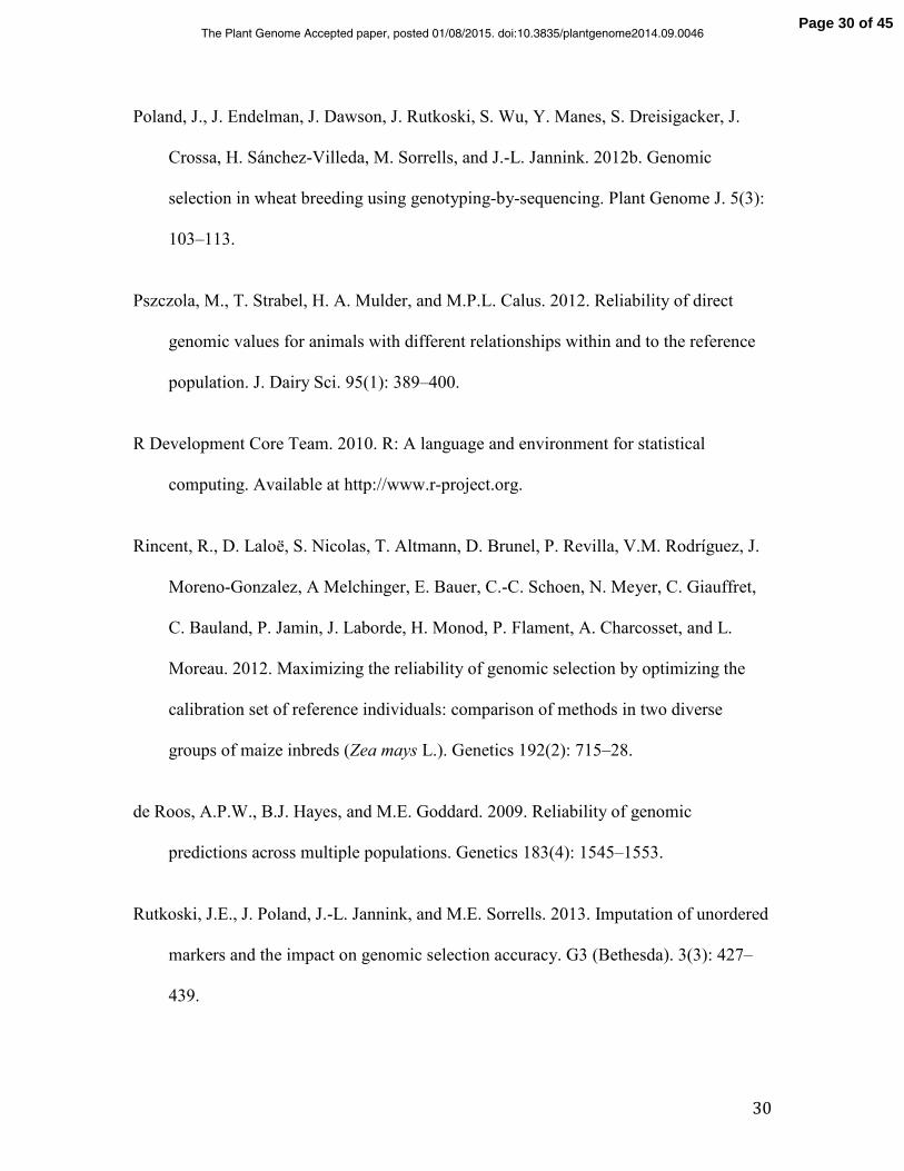
The historical and SC populations were significantly differentiated based on the

median Fst across all markers, p-value = 0. Populations also formed distinct but partially

overlapping groups together based on the first two principle components calculated from


16

the genetic relationship matrix (Figure 1). The rate of LD decay with physical distance

was similar for the historical and SC population, however there was more long-range LD

in the SC population (Figure 2).

TP comparison and optimization

TPPS always lead to higher accuracies than TPH and for Np= 73 and 146

accuracies were significantly different (Figure 3). As Np increased, the difference

between accuracies from TPPS and TPH decreased. For example, when Np =73, TPPS was

4.4 times more accurate than TPH, and when Np =292, TPPS was only 1.5 times more

accurate than TPH. For TPH, optimally selected TPs lead to significantly higher

accuracies than randomly selected TPs for Np= 73, 146, 219, and 292 (Figure 4). The

optimization criteria PEVmean and CDmean performed similarly and both outperformed

Fst. For Np= 73, 146, 219, and 292 optimally selected TPs based on PEVmean and

CDmean lead to accuracies higher than that of the full TP with Np= 365.

When validated using a second population derived from the SC population, the

TPs that were optimally selected from TPH based on CDmean and PEVmean lead to

consistently higher accuracies compared to randomly selected TPs (Figure 5). For this

validation experiment, the improvement in accuracy provided by CDmean optimization

was most consistent, followed by PEVmean. The TPs selected based on Fst performed

worse than random TPs for Np= 146 and 219. Although optimized TPs selected using

CDmean or PEVmean consistently outperformed random TPs, no significant differences

were detected due to the large variation of the random TP accuracies due to sampling. In


17

contrast with the results from validation using the SC population, we observed increasing

accuracy as Np increased for TPs optimized using CDmean and PEVmean. However,

when Np=292 and TPs were selected based on Fst, PEVmean, or CDmean; and when

Np=73 and TPs were selected based on Fst, accuracy was higher than that of the complete

TP.

Combined TP analysis

When WX�Y� of TPPS was low (H2 = 0.2) adding samples from TPH of WX�Y� = 0.3,

0.4, and 0.6, led to a small, but constant improvement in accuracy as Np increased

(Figure 6). When WX�Y� of TPH was also low (H2 = 0.2) adding individuals from TPH to

TPPS led to an initial decrease in accuracy, followed by a slight increase with increasing

Np. For the maximum number of TPH samples added, 365, accuracy improved by 1.2%,

7.6%, 10.9%, and 11.9% for WX�Y� =0.2, 0.3, 0.4, and 0.6, respectively. Adding a weight of

1-WX�Y� to the diagonal of the residual covariance only affected accuracy by up to 1.02%

(Figure 6, panel B).

When WX�Y� of TPPS was high, 0.6 (Figure 7), adding samples from TPH of equal

heritability led to small and constant increases in accuracy with increasing Np. When

WX�Y� of added samples from TPH was moderate, 0.3 and 0.4, there was an initial decrease

in accuracy, followed by a slow increase with increasing Np. However, even for the

largest Np, 365, adding individuals from TPH led to a -4.5% and 0% change in accuracy

for WX�Y� = 0.3 and 0.4, respectively. When WX�Y� of added samples from TPH was low, 0.2,

accuracy declined by 12% and did not show an eventual increase with increasing Np.


18

Adding a weight of 1-WX�Y� to the diagonal of the residual led to improved accuracy when

WX�Y� of TPH was 0.2, 0.3, and 0.4 (Figure 7, panel B). Improvements in accuracy due to

weighting ranged from 2.4% to 9.7%. The lower the WX�Y� of TPH, the greater the benefit

of using TP specific weights. However when WX�Y� of TPH was very low at 0.2, adding

individuals from TPH never led to a net increase in accuracy, even when weighing was

used.

In summary, using TPH individuals when TPPS individuals were available for

training was always beneficial when WX�Y� of TPH was greater than WX�Y� of TPPS. In some

cases, whenWX�Y� of TPPS was high and WX�Y� of TPH was at least moderate, using TPH and

TPPS individuals for training was beneficial when observations were properly weighted

according to the heritability of their TP of origin.

Discussion

Populations

The significant population differentiation between the historical and selection

candidate populations was a consequence of selection and genetic drift that occurred

because the SC population was generated from only fourteen founder lines from the

historical population that were selected because they had at least moderate stem rust

resistance and good agronomic performance. Selection and drift lead to a reduced rate of

LD decay with physical distance in the SC population. The level of differentiation

between historical and selection candidate populations due to selection and drift would be


19

expected in plant breeding programs because each cycle of selection is founded by a

small number of parents selected for intermating. However, breeding programs that use a

lower selection intensity may experience less differentiation between historical and

selection candidate populations. Thus, breeding programs with lower selection intensities

may be able to use historical data more successfully compared those that use higher

selection intensities.

Accuracy comparison

In general, the relative performance of a historical and population specific TP

depends on the relative population sizes, trait heritability, levels of GxE, and genetic

differentiation between the historical TP and the SCs. In this study, the lower accuracy

from TPH was primarily driven by the genetic differentiation between TPH and the

validation set. Accuracy from a historical TP could be as high or higher than that of a

population specific TP in some scenarios. For example, based on linear regression of

accuracy on TP size for both TPPS and TPH, if we were to add 225 more historical

individuals to TPH, TPPS and TPH accuracies may have been equivalent. Furthermore, if

this study focused on a trait such as yield with low heritability on a single plot basis and

high GxE, population specific training data from very few environments will be of low

line mean heritability and may not adequately sample the target environments of the

breeding program. Lastly, a historical TP would likely be more effective if it has not

undergone selection and subsequently a reduction in genetic variance (Bulmer, 1971) for


20

the trait of interest. However, it may not be possible to find historical data from a

breeding program where traits of interested have not undergone selection.

Training population optimization

The TP optimization methods based on PEVmean and CDmean enabled the

selection of TPs from TPH that were more accurate than those selected based on random

sampling. Other studies evaluating TP optimization (Isidro et al. 2014; Rincent et al.

2014) found similar results; however according to Isidro et al. (2014), TP optimization

could be less accurate than random sampling if it resulted in a reduction in the phenotypic

variance. TP optimization would be useful if the historical dataset used for model training

does not contain phenotypic data for all traits of interest. A subset of individuals from a

historical dataset, selected to be predictive of the selection candidates based on CDmean

or PEVmean, could be phenotyped for new traits of interest. This could reduce costs with

potentially little to no sacrifice in accuracy compared to phenotyping all historical

individuals.

Optimizing with respect to population progenitors appeared to be an effective way

to select the appropriate subsample individuals for phenotyping and model updating in a

GS progam, however, the Np that leads to the highest accuracy cannot be identified in

advance. If phenotyping resources are limited, one could select Np based on resource

constraints, and select individuals for phenotyping and model updating by optimizing

with respect to the progenitors of the future SCs.


21

Interestingly, some optimal TPs lead to greater accuracy compared to the

complete TP, suggesting that TP optimization could increase the overall GS prediction

accuracy if it were possible to know in advance what Np value could maximize accuracy.

However, we caution that the ability to select an optimal TP that leads to greater accuracy

compared to the complete TP is expected to be highly dependent on a given population

and trait due to differences in population and family structure, non-additive genetic

variance, and LD between markers and causal loci. Assuming there is perfect linkage

between markers and QTL, increasing Np values will lead to an asymptotic increase in

accuracy (Daetwyler et al., 2010; de Los Campos et al., 2013), and the complete TP will

lead to higher accuracy than an optimal subset of the TP. Assuming imperfect linkage

between markers and QTL and population or family structure, optimizing the TP for the

SCs could increase accuracy because the estimated relationships between pairs of closely

related individuals will be more accurate than the estimated relationships between less

related individuals (de Los Campos et al., 2013), and eliminating less related individuals

could reduce noise in the relationship matrix. Aside from population genetic factors, the

importance of non-additive genetic variance for the trait of interest may also partially

determine if TP optimization improves accuracy. Non-additive genetic variance

contributes to the covariance among close relatives only. When the TP is selected to be

closely related to the SCs, more non-additive genetic variance may be captured in G-

BLUP, thus for traits where non-additive genetic variance is important, TP optimization

may lead to higher accuracy compared to the complete TP. This is similar to the effect of

using a Gaussian kernel, where the genetic covariance can decrease more rapidly with

genetic distance (Endelman, 2011). However with optimization, the relationship between


22

some pairs of individuals is effectively set to zero. Because of the various factors that

affect the potential gain from training with an optimized TP rather than the complete TP,

selecting optimal subsets from a TP is not yet a reliable way to improve accuracy.

Combining training population data sources

Our results showed that retaining historical data when data on close relatives was

available reduced accuracy especially when the heritability of the historical data was low,

the heritability of the close relative training data was high, and the observations were not

weighted properly according to heritability. This has implications for prediction model

updating. In a selection program, it may be better to discard older training data that is less

relevant to the selection candidates as newer training data becomes available. However,

when to discard training data will need to be determined empirically because it will

depend on the selection intensity of the breeding program, the availability of data on

close relatives, and quality of the historical data. For example, Asoro et al. (2011)

evaluated the utility of adding historical oat lines to a training population going back in

time and found that historical lines did not decrease accuracy, though the increase in

accuracy they provided was small.

Conclusion

This case study found that historical data could be useful for initializing a GS

based breeding program where the selection candidates are founded by historical


23

individuals. Although the highest accuracy could be achieved by phenotyping and model

training with a subset of the selection candidate population itself, such an approach would

require at least two years of additional time to collect multi-location and multi-year data

for all traits of interest, and may be less robust to GxE effects because data will be

collected across relatively few environments. While historical data may be useful

initially, this study suggests that once GS model updating can occur, it may be best to

discard historical data and simply use the most recent data for model training.

Optimization of the historical TP was promising for selection of data subsets that

were more predictive than randomly selected subsets. This would be useful when using a

historical TP that lacks data for some key traits. To save resources, a subset of the

historical TP, rather than the entire TP, could be phenotyped while the selection

candidates are being developed.

We note that our conclusions are relevant to the germplasm and trait used in this

study, and individual breeding programs will need to initiate GS programs in order to

empirically determine the utility of historical data, and at what point data should be

discarded from the model training dataset. The utility of TP optimization should also be

empirically studied in the context of a GS breeding program. More publicly available

data generated by GS selection experiments and breeding programs will enable many

such studies that will lead to the discovery of common trends across datasets.

Supplemental information available

Supplemental material is available at http://www.crops.org/publications/tpg.


24

Supplemental File S1. Genotyping-by-sequencing data for the historical and SC

popualtions

Supplemental File S2: Phenotypic data for the historical and SC populations

Acknowledgements

This research was funded by The Bill and Melinda Gates Foundation (grants: Durable

Rust Resistance in Wheat and Genomic Selection: The Next Frontier For Rapid Gains in

Maize And Wheat Improvement), the United States Department of Agriculture-

Agricultural Research Service (USDA-ARS) (Appropriation No. 5430-21000-006-00D),

USDA National Institute of Food and Agriculture (NIFA)- Agriculture and Food

Research Initiative (AFRI) grant support award number 2011-68002-30029, and United

States Agency for International Development (USAID) support to the Feed the Future

Innovation Lab for Applied Wheat Genomics (Cooperative Agreement No. AID-OAA-A-

13-00051). Partial support for J. Rutkoski was provided by a USDA National Needs

Fellowship Grant #2008- 38420-04755 and an American Society of Plant Biology

(ASPB) -Pioneer Hi-Bred Graduate Student Fellowship. Partial support was also

provided by USDA-NIFA Hatch Project 149-430. Mention of trade names or commercial

products in this publication is solely for the purpose of providing specific information

and does not imply recommendation or endorsement by the USDA. USDA is an equal

opportunity provider and employer.


25


26

References

Amin, N., C.M. van Duijn, and Y.S. Aulchenko. 2007. A genomic background based

method for association analysis in related individuals. PLoS One 2(12): e1274.

Asoro, F.G., M. A. Newell, W.D. Beavis, M.P. Scott, Tinker, N. A. and J.-L. Jannink.

2011. Accuracy and training population design for genomic selection on quantitative

traits in elite North American oats. Plant Genome J. 4(2): 132–144.

Astle, W., and D.J. Balding. 2009. Population structure and cryptic relatedness in genetic

association studies. Stat. Sci. 24(4): 451–471.

Bates, D., and M. Maechler. 2010. lme4: Linear mixed-effects models using S4 classes.

Available at http://cran.r-project.org/package=lme4.

Beeck, C.P., W. A. Cowling, A. B. Smith, and B.R. Cullis. 2010. Analysis of yield and

oil from a series of canola breeding trials. Part I. Fitting factor analytic mixed

models with pedigree information. Genome 53(11): 992–1001.

Bernardo, R. 1994. Prediction of maize single-cross performance using RFLPs and

information from related hybrids. Crop Sci. 34(1): 20–25.

Box, G.E., and D.R. Cox. 1964. An analysis of transformations. J. R. Stat. Soc. Ser. B

26(2): 211–252.

Bulmer, M.G. 1971. The Effect of selection on genetic variability. Am. Nat.

105(943):201-211.


27

Crossa, J., G.D.L. Campos, P. Pérez, D. Gianola, J. Burgueño, J.L. Araus, D. Makumbi,

R.P. Singh, S. Dreisigacker, J. Yan, V. Arief, M. Banziger, and H.-J. Braun. 2010.

Prediction of genetic values of quantitative traits in plant breeding using pedigree

and molecular markers. Genetics 186(2): 713–724.

Daetwyler, H.D., R. Pong-Wong, B. Villanueva, and J. A. Woolliams. 2010b. The impact

of genetic architecture on genome-wide evaluation methods. Genetics 185(3): 1021–

1031.

Dawson, J.C., J.B. Endelman, N. Heslot, J. Crossa, J. Poland, S. Dreisigacker, Y. Manès,

M.E. Sorrells, and J.-L. Jannink. 2013. The use of unbalanced historical data for

genomic selection in an international wheat breeding program. F. Crop. Res. 154:

12–22.

Elshire, R.J., J.C. Glaubitz, Q. Sun, J. A. Poland, K. Kawamoto, E.S. Buckler, and S.E.

Mitchell. 2011. A robust, simple genotyping-by-sequencing (GBS) approach for

high diversity species. PLoS One 6(5): e19379.

Endelman, J.B. 2011. Ridge regression and other kernels for genomic selection with R

package rrBLUP. 4(3): 250–255.

Garrick, D.J., J.F. Taylor, and R.L. Fernando. 2009. Deregressing estimated breeding

values and weighting information for genomic regression analyses. Genet. Sel. Evol.

41: 55.


28

Gilmour, A.R., B.J. Gogel, B.R. Cullis, and R. Thompson. 2009. ASReml user huide

release 3.0.

Goddard, M. 2009. Genomic selection: prediction of accuracy and maximisation of long

term response. Genetica 136(2): 245–257.

Habier, D., R.L. Fernando, and J.C.M. Dekkers. 2007. The impact of genetic relationship

information on genome-assisted breeding values. Genetics 177(4): 2389–2397.

Haley, C. S., and Visscher, P. M. 1998. Strategies to utilize marker-quantitative trait loci

associations. J. Dairy Sci. 81(2): 85–97.

Hallauer, A.R., M.J. Carena, and J.B. Miranda F. 2010. Quantitative genetics in maize

breeding. Iowa State University Press, Ames, IA.

Hayes, B.J., P.M. Visscher, and M.E. Goddard. 2009. Increased accuracy of selection by

using the realized relationship matrix. Genet. Res. (Camb). 91(1): 47–60.

Henderson, C.R. 1984. Applications of linear models in animal breeding. University of

Guelph Press, Guelph, Ontario, Canada.

Isidro, J., J-L. Jannink, D. Akdemir, J. Poland, N. Heslot, M.E. Sorrells. 2014. Training

set optimization under population structure in genomic selection. Theor. Appl.

Genet.

Kennedy, B.W., and D. Trus. 1993. Considerations on genetic connectedness between

management units under an animal model. J. Anim. Sci. 71(9): 2341–2352.


29

Laloë, D. 1993. Precision and information in linear models of genetic evaluation. Genet.

Sel. Evol. 25(6): 1–20.

Leutenegger, A.-L., B. Prum, E. Génin, C. Verny, A. Lemainque, F. Clerget-Darpoux,

and E. A. Thompson. 2003. Estimation of the inbreeding coefficient through use of

genomic data. Am. J. Hum. Genet. 73(3): 516–23.

Long, N., D. Gianola, G.J.M. Rosa, and K.A. Weigel. 2011. Long-term impacts of

genome-enabled selection. J. Appl. Genet.: 467–480.

De Los Campos, G., A.I. Vazquez, R. Fernando, Y.C. Klimentidis, and D. Sorensen.

2013. Prediction of complex human traits using the genomic best linear unbiased

predictor. PLoS Genet. 9(7): e1003608.

Meuwissen, T.H.E., B.J. Hayes, and M.E. Goddard. 2001. Prediction of total genetic

value using genome-wide dense marker maps. Genetics 157(4): 1819–1829.

Peterson, R.F., A.B. Campbell, and A.E. Hannah. 1948. A diagrammatic scale for

estimating rust intensity on leaves and stems of cereals. Can. J. Res. 26c(5): 496–

500.

Piepho, H.P. 2009. Ridge regression and extensions for genomewide selection in maize.

Crop Sci. 49(4): 1165–1176.

Poland, J. A., P.J. Brown, M.E. Sorrells, and J.-L. Jannink. 2012a. Development of high-

density genetic maps for barley and wheat using a novel two-enzyme genotyping-

by-sequencing approach. PLoS One 7(2): e32253.


30

Poland, J., J. Endelman, J. Dawson, J. Rutkoski, S. Wu, Y. Manes, S. Dreisigacker, J.

Crossa, H. Sánchez-Villeda, M. Sorrells, and J.-L. Jannink. 2012b. Genomic

selection in wheat breeding using genotyping-by-sequencing. Plant Genome J. 5(3):

103–113.

Pszczola, M., T. Strabel, H. A. Mulder, and M.P.L. Calus. 2012. Reliability of direct

genomic values for animals with different relationships within and to the reference

population. J. Dairy Sci. 95(1): 389–400.

R Development Core Team. 2010. R: A language and environment for statistical

computing. Available at http://www.r-project.org.

Rincent, R., D. Laloë, S. Nicolas, T. Altmann, D. Brunel, P. Revilla, V.M. Rodríguez, J.

Moreno-Gonzalez, A Melchinger, E. Bauer, C.-C. Schoen, N. Meyer, C. Giauffret,

C. Bauland, P. Jamin, J. Laborde, H. Monod, P. Flament, A. Charcosset, and L.

Moreau. 2012. Maximizing the reliability of genomic selection by optimizing the

calibration set of reference individuals: comparison of methods in two diverse

groups of maize inbreds (Zea mays L.). Genetics 192(2): 715–28.

de Roos, A.P.W., B.J. Hayes, and M.E. Goddard. 2009. Reliability of genomic

predictions across multiple populations. Genetics 183(4): 1545–1553.

Rutkoski, J.E., J. Poland, J.-L. Jannink, and M.E. Sorrells. 2013. Imputation of unordered

markers and the impact on genomic selection accuracy. G3 (Bethesda). 3(3): 427–

439.


31

Thompson, R., B. Cullis, , A. Smith, , and A. Gilmour. 2003. A sparse implementation of

the average information algorithm for factor analytic and reduced rank

variance models. Aust. NZ. J. Stat. 45(4): 445–459.

Weir, B., and C. Cockerham. 1984. Estimating F-statistics for the analysis of population

structure. Evolution, 38(6): 1358–1370.

Yu, L.-X., A. Lorenz, J. Rutkoski, R.P. Singh, S. Bhavani, J. Huerta-Espino, and M.E.

Sorrells. 2011. Association mapping and gene-gene interaction for stem rust

resistance in CIMMYT spring wheat germplasm. Theor. Appl. Genet. 123(8): 1257–

1268.

Zadoks, J., T. Chang, C. F. Konzak, 1974. A decimal code for the growth stages of

cereals. Weed. Res., 14:415–421.


32

Figure 1: Principal components analysis including the historical lines, SCs, and SC

parents.


33

Figure 2: Relationship between linkage disequilibrium measured as r2 and genetic

distance in centimorgans (cM) for historical and SC populations.


34

Figure 3: Prediction accuracies for the SC population based on TPPS and TPH with

varying population sizes.


35

Figure 4: Prediction accuracies for the SC population based on optimized TPs from TPH

in comparison with accuracies from randomly sampled TPs from TPH. The 95%

confidence interval for accuracy from randomly sampled TPs is shaded in grey.


36

Figure 5: Prediction accuracies for an additional validation population based on

optimized TPs from TPH in comparison with accuracies from randomly sampled TPs

from TPH. The 95% confidence interval for accuracy from randomly sampled TPs is

shaded in grey.


37

Figure 6: The effect of adding TPH individuals to TPPS when simulated heritability of

TPPS is 0.2 and simulated heritability of TPH is 0.2, 0.3, 0.4, and 0.6. A) Populations are

weighted equally, B) populations weighted according to simulated heritability.


38

Figure 7: The effect of adding TPH individuals to TPPS when simulated heritability of

TPPS is 0.6 and simulated heritability of TPH is 0.2, 0.3, 0.4, and 0.6. A) Populations are

weighted equally, B) populations weighted according to simulated heritability.


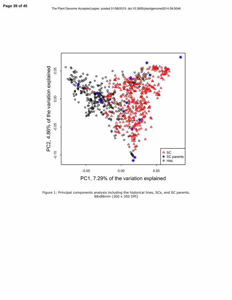
Figure 1: Principal components analysis including the historical lines, SCs, and SC parents.

88x88mm (300 x 300 DPI)


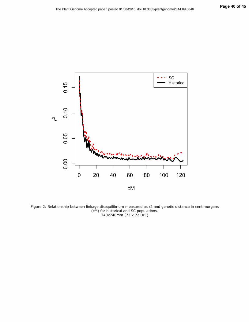
Figure 2: Relationship between linkage disequilibrium measured as r2 and genetic distance in centimorgans (cM) for historical and SC populations.

740x740mm (72 x 72 DPI)


Figure 3: Prediction accuracies for the SC population based on TPPS and TPH with varying population sizes. 81x81mm (300 x 300 DPI)


Figure 4: Prediction accuracies for the SC population based on optimized TPs from TPH in comparison with accuracies from randomly sampled TPs from TPH. The 95% confidence interval for accuracy from randomly

sampled TPs is shaded in grey.

1270x1270mm (72 x 72 DPI)


Figure 5: Prediction accuracies for an additional validation population based on optimized TPs from TPH in comparison with accuracies from randomly sampled TPs from TPH. The 95% confidence interval for accuracy

from randomly sampled TPs is shaded in grey.

1270x1270mm (72 x 72 DPI)


Figure 6: The effect of adding TPH individuals to TPPS when simulated heritability of TPPS is 0.2 and simulated heritability of TPH is 0.2, 0.3, 0.4, and 0.6. A) Populations are weighted equally, B) populations

weighted according to simulated heritability.

114x85mm (300 x 300 DPI)


Figure 7: The effect of adding TPH individuals to TPPS when simulated heritability of TPPS is 0.6 and simulated heritability of TPH is 0.2, 0.3, 0.4, and 0.6. A) Populations are weighted equally, B) populations

weighted according to simulated heritability.

114x85mm (300 x 300 DPI)


Efficient use of historical data for genomic selection: … · resistance in wheat J. Rutkoski1,...

Documents

Transcript of Efficient use of historical data for genomic selection: … · resistance in wheat J. Rutkoski1,...