Scientific Bulletin of the Politehnica University of Timisoara

Transactions on Mechanics Special issue

The 6th International Conference on Hydraulic Machinery and Hydrodynamics Timisoara, Romania, October 21 - 22, 2004

EFFICIENT SOLUTIONS OF THE EULER AND NAVIER-STOKES EQUATIONS FOR EXTERNAL FLOWS

Dan MATEESCU

Professor, Aerospace Program Director Department of Mechanical Engineering

McGill University, Montreal, Canada 817 Sherbrooke Street West, Montreal, Quebec, H3A 2K6, Canada

Email: dan.mateescu@mcgill.ca

ABSTRACT This invited paper presents efficient solutions of the Euler and Navier-Stokes equations based on finite difference and finite volume formulations. They were obtained with several methods recently developed for the efficient analysis of steady and unsteady external flows. (i) A biased-flux method based on an explicit finite volume formulation is first presented for the solution of the Euler equations. A second-order scheme is used for the flux calculation with an upwind or downwind bias for the flow variables, according to the subsonic or supersonic character of the local flow. The method is first validated for compressible flows with expansions and shock waves in nozzles, and then used to obtain solutions for subsonic, transonic and supersonic flows past airfoils. (ii) Efficient Navier-Stokes solutions are also presented for the flows past airfoils at low Reynolds numbers, dominated by viscous effects, which are of interest for micro-aircraft and unmanned air vehicle applications.

KEYWORDS Aerodynamics, steady and unsteady flows, inviscid and viscous flows, computational fluid dynamics.

1. INTRODUCTION The numerical methods of solutions used in the

analysis of steady and unsteady flows of engineering interest have to be characterized by a very good computational efficiency in addition to a very good accuracy. The requirement of a good computational efficiency and a user-friendly implementation is important especially in the study of steady and unsteady fluid-structure interaction problems, which requires the simultaneous solution of the Euler or Navier-Stokes equations in conjunction with the equations of the deformation motion of the structures subjected to fluid flows.

This paper presents efficient methods based on

finite difference and finite volume formulations recently developed by this author and collaborators for the analysis of steady and unsteady flows with fixed and oscillating boundaries in subsonic, transonic and supersonic flow regimes [15, 20, 21, 22, 24-27]. Other efficient methods using Lagrangian and spectral formulations [18, 23, 28] are presented in other papers [16, 17].

An efficient biased-flux method, based on an explicit finite volume formulation, is first presented for the solution of the Euler equations in subsonic, transonic and supersonic flows. This method takes into account the physical direction of perturbation propagation in compressible flows, avoiding thus the numerical problem of the odd-and-even-points decoupling which appears in other methods with negative effects on the computational efficiency.

A special research interest has recently been devoted to the analysis of the flows at low and very low Reynolds numbers past airfoils and wings. This interest is driven by micro-aerial-vehicles (MAV) and unmanned air vehicles (UAV) applications, which were made possible by the recent advances in micro-electro-mechanical systems (MEMS). These applications have shown that many questions are unanswered regarding the airfoil aerodynamics at low Reynolds numbers. The flows past airfoils at low Reynolds numbers are dominated by viscous effects, transitional and flow separation phenomena, which complicate the understanding of airfoil aerodynamics in these conditions.

Accurate solutions for the low Reynolds number flows past airfoils are also presented in this paper by efficiently solving the Navier-Stokes equations using a finite difference method using artificial compressibility.

2. BIASED FLUX METHOD FOR SOLVING THE EULER EQUATIONS IN SUBSONIC, TRANSONIC AND SUPERSONIC FLOWS

The explicit or implicit finite volume methods are directly applied on structured or unstructured grids without the need of coordinate transformation. Numerous methods have been developed based on various numerical discretizations of the flux derivatives, such as those developed by Jameson et al. [8, 37] and MacCormack et al. [12]. These basic methods, as well as many other similar methods not mentioned here, were proven to be efficient and reliable in solving various engineering problems. However, in this class of methods, the numerical procedure does not reflect the physical propagation of perturbations, with eventual negative implications on the numerical stability and convergence, accuracy and ability to avoid numerical distortions in capturing sharp shocks.

To overcome this deficiency, several numerical methods have been developed to better reflect the physical propagation of perturbations. However, these methods become very involved for multidimensional flows (as in the methods developed by Roe [35], or based on flux splitting [1]), with negative implications on the computational efficiency; or the basic model developed for quasi 1D flows has no more the same physical significance for multidimensional flows (as in the case of Godunov’s method [6]).

A more accurate flux calculation using discretized forms of the Euler equations, and taking into account the permissible directions of perturbation propagation in compressible flows, has been developed by Mateescu & Lauson [30].This method led to very accurate and computationally efficient solutions; however, the numerical scheme became more involved for multi-dimensional flows, especially in the presence of the shock waves.

The explicit biased flux method, developed in [24], uses a relatively simple numerical scheme to efficiently take into account the physical propagation of perturbations, by using an upwind and downwind bias in the evaluation of fluxes in function of the local flow Mach number. This method can be easily applied to multi-dimensional flows.

2.1. Problem formulation An explicit finite volume formulation is used in this method, in which the Euler equations for rotational compressible flows are expressed in the form

( )[ ] 0gnVff =+⋅+∂∂

∫∫ ∂VVV Add

t, (1)

where and V V∂ represent the finite control volume and its bounding surface, and where

{ }T,, Eρρρ Vf = , (2) ( ){ }T,,0 nVng ⋅= pp , (3)

in which ρ , and p wvu kjiV ++= are the fluid density, pressure and velocity, is the outward unit vector normal to the bounding surface

zyx nnn kjin ++=

V∂ . For 2D flows, the computational domain is

discretized into a certain number of quadrilateral cells, , each of these cells being characterized by an area (corresponding to the volume in 3D) and by its bounding contour

formed by four straight lines denoted by the subscripts

ji NN ×

jiA

jiA∂( )ji ,21± and ( 21, ±ji ) , characterized

by their Cartesian projections jix ,21±∆ , jiy ,21±∆ and

21, ±∆ jix , 21, ±∆ jiy (absolute values). In this case, the Euler equations in matrix form can be discretized as

( )fQf

jiji

t−=

∂

∂ , (4)

where is the cell-averaged value of the state vector

jif

f and ( )fQ ji is the flux operator defined as

{ }T,,, Evu ρρρρ=f , (5)

( ) [ ]21,21,,21,211

−+−+ −+−= jijijijiji

ji AHHHHfQ (6)

in which ( ) ( )12V2 −+= γρpE is the specific energy per unit of mass, and

lklklklklk xy ,,,,, ∆−∆= GFH , (7)

( ) ⎥⎥⎥⎥⎥

⎦

⎤

⎢⎢⎢⎢⎢

⎣

⎡

+

+=

lklklklk

lklklk

lklklk

lklk

lk

upEvu

puu

,,,,

,,,

,2

,,

,,

,

ρρ

ρρ

F , (8a)

( ) ⎥⎥⎥⎥⎥

⎦

⎤

⎢⎢⎢⎢⎢

⎣

⎡

++

=

lklklklk

lklklk

lklklk

lklk

lk

vpEpv

uvv

,,,,

,2

,,

,,,

,,

,

ρρρρ

G . (8b)

The flux vectors and G at the cell interfaces have to be expressed in terms of the cell-averaged values of the state vector

F

f , in order to iteratively solve by time marching the explicit Euler equations (4). The manner in which the interface values are related by the cell-averaged values distinguishes the numerous finite volume methods developed by

various authors. Thus, in the method developed by Jameson and his collaborators [8, 37], the fluxes at an interface are calculated by using an algebraic mean of the cell-averaged values of the two neighboring cells, such as ( ) 2,,1,21 jijiji fff += ±± , or

( ) 2,,1,21 jijiji FFF += ±± . This very simple approach led to robust

algorithms, which have been successfully used to solve various aerodynamic problems. However, this flux calculation leads to the odd-and-even-points decoupling (most obvious in the case of rectangular cells, where the flow variable changes for the odd-numbered cells depend only on the flow variables in the even-numbered cells, and vice-versa). To avoid this problem, an artificially-added dissipation, involving second and fourth order terms, has been ingeniously developed by Jameson [8, 37]. This artificially-added dissipation implies, however, a heavy computational effort, especially to calculate the fourth-order dissipation terms, undermining thus the efficiency of the simple interface-fluxes algorithm. Also, due to this added dissipation, the captured shocks are less sharp.

In addition, the flux variables calculated at an interface in this manner always depend on both sets of flow variables in the upwind and downwind neighboring cells, and this does not correspond to the actual directions of perturbation propagation in compressible flows. For example, the perturbations propagate in quasi 1D flow with the characteristic velocities , and (where is the speed of sound), which are all positive for supersonic flows ( ); in this case, the flux values depend only on the upstream flow variables, and obviously not on the downstream ones, as obtained in the flux calculation based on algebraic averaging.

au − u au + a

au >

2.2. Method of solution In the biased-flux developed in [24], the flux values are calculated using simple weighted expressions involving the upwind and downwind cells, such as

( ) jijijijiji ,1,,,,21 1 +ρρ

+ ρα−+ρα=ρ , (9a) ( ) ji

ujiji

ujiji uuu ,1,,,,21 1 ++ α−+α= , (9b)

( ) jiv

jijiv

jiji uuv ,1,,,,21 1 ++ α−+α= , (9c) ( ) ji

pjiji

pjiji ppp ,1,,,,21 1 ++ α−+α= , (9d)

where the values of the weighting parameters , , and are taken between 0 and 1 in

function of the subsonic or supersonic character of the local flow.

ρα ji ,

uji ,α v

ji ,α pji ,α

A subsonic quasi 1D nozzle flow is physically and mathematically well defined by specifying the stagnation pressure and temperature (or speed of sound) at the inlet and the static pressure at the outlet. In contrast, a supersonic quasi 1D nozzle flow is well defined by specifying all flow variables at the inlet (and no condition at the outlet).

By analogy with the nozzle flow, at any interface between two cells, the static pressure has to be characterized by a downwind bias in a locally subsonic flow, which can be modeled by considering lower values for the weighting parameter (such as 0.1 to 0.4), and by an upwind bias in a locally supersonic flow, modeled by considering higher values for , (such as 0.6 to 0.9). At the same time, the other fluid dynamic variables,

0, α=α pji

1, α=α pji

ρ , and , have an upwind bias at the interface in both subsonic and supersonic local flows, modeled by higher values of the weighting parameters . The optimum values for the upwind- and downwind-biased parameters, and , were found by numerical experimentations to be in the range 0.75 – 0.8 and, respectively, 0.2 - 0.25. The numerical results presented in this paper have been obtained with and .

u v

1,,, α=α=α=α ρ vji

ujiji

1α 0α

75.01 =α 25.00 =αAs a result of this upwind-downwind biased flux

calculation, this method does not present the odd-and-even-points decoupling, and hence there is no need for a fourth-order artificially-added dissipation for subsonic and supersonic flows; this enhances considerably the computational efficiency of the biased-flux method.

For the flows involving shock waves, a second-order dissipation is added only in the vicinity of the shock, which is detected using a sensor based on a normalized second-order difference of the pressure, as that used by Jameson et al. [8]; for example, in the case of quasi 1D flows,

jiν

( )1111 22 −+−+ +++−=ν iiiiiii pppppp . (10) Thus the flux operator is augmented by a

second-order dissipation term in the form ( )fQ ji

( )fjiD

( ) [ 21,21,,21,211

−+−+ −+−= jijijijiji

ji AHHHHfQ

( )]fjiD− , (11) where

( ) fffff 21,21,,21,21 −+−+ +++= jijijijiji ddddD , (12) in which, for example,

( )jijijijid ,,1)2(

,21,21 fff −= +±±± ε , (13)

where ( )jijiji k ,12)2(

,21 ,max ±± = ννε , with 2 having a typical value of 1/4. This second-order dissipation does not essentially affect the computational efficiency, since its application is restricted only to the flows with shock waves, and in this case only to very narrow regions (several cells wide) in the vicinity of the shocks detected by the sensor ν .

k

ji

Equation (16) is then solved by explicit iterations with a fourth-order Runge-Kutta scheme, similar to that used in [8], which can be expressed for the pseudo-time levels and in the form nt ttt nn ∆+=+1

( ) ( )nji

njiji t fQff 2)1( ∆−= , (14a)

( ) ( ))1()2( 2 fQff jinjiji t∆−= , (14b)

), (14c) ( )2()3( fQff jinjiji t∆−=

( ) ( ) ([ )1()1( 26 fQfQff jin

jinji

nji t +∆−=+ )

( ) ( )])3()2(2 fQfQ jiji ++ , (14d)

2.3. Method validation The method is first validated for quasi 1D flow in

a circular-arc-bump nozzle. The present solution, which did not require any artificial dissipation, was found in very good agreement with the exact solution obtained for this quasi 1D flow as shown in Figure 1; also shown is the solution obtained with Jameson’s method [8] using artificially-added dissipation, which required 33% more computing time per iteration than the present biased-flux method (CFL number was 2.1 in both methods).

Figure 1. Mach number variation in a circular-arc-bump nozzle (quasi 1D flow).

2.4. Solutions for 2D subsonic, transonic and supersonic confined flows

The solutions obtained with the biased-flux method for the 2D subsonic, transonic and supersonic flows in the same circular-arc-bump nozzle are shown in Figures 2, 3 and 4.

Figure 2. Subsonic nozzle flow. Mach number distributions on the lower and upper walls and

iso-Mach lines. Comparison with [33].

Figure 3. Transonic nozzle flow. Mach number distributions on the lower and upper walls and

iso-Mach lines. Comparison with [5].

Figure 4. Supersonic nozzle flow. Mach number distributions on the lower and upper walls and

iso-Mach lines. Comparison with [5].

2.5. Subsonic, transonic and supersonic airfoil flows

Solutions for the subsonic, transonic and supersonic flows have been also obtained with the biased flux methods. The present solutions computed for the pressure distributions on the NACA 0012 airfoil are compared in Figures 5 and 6 with the experimental results obtained in [39] for subsonic flow (at Mach number and angle of attack ) and for transonic flow (at Mach number and angle of attack

). The present solutions were found in good agreement with the experimental results.

503.0=∞Mo25.1=α

8.0=∞Mo05.6=α

-1.50

-1.00

-0.50

0.00

0.50

1.00

1.50

2.00

2.50

0.00 0.20 0.40 0.60 0.80 1.00x/chord

-Cp Present solutionExperiment[13]

-1.50

-1.00

-0.50

0.00

0.50

1.00

1.50

0.00 0.20 0.40 0.60 0.80 1.00x/chord

-CpPresent SolutionPulliam's Compt. Results[14]

Figure 6. Pressure coefficient distribution on the NACA 0012 airfoil at and .

Comparison with experiments [39]. 8.0=∞M o05.6=α

Figure 7. Mach number distribution on the NACA 0012 airfoil and its symmetry-axis extension

at and , and the isobar lines. 2.1=∞M o0=α

Figure 5. Pressure coefficient distribution on the NACA 0012 airfoil at and .

Comparison with experiments [39]. 503.0=∞M o25.1=α

variety of applications ranging from domestic windmills to special military aircraft and unmanned air vehicles (UAV), which were made possible by the recent advances in the micro-electro-mechanical-systems (MEMS). Very small aircrafts called micro-aerial-vehicles (MAV) can operate in various environments including tunnels, desert and jungle (for examples see references included in [15]). These applications have shown that many questions are unanswered regarding the airfoil aerodynamics at low and very low Reynolds numbers. The flows past airfoils at low Reynolds numbers are dominated by viscous effects, transitional and flow separation phenomena, which complicate the understanding of airfoil aerodynamics in these conditions.

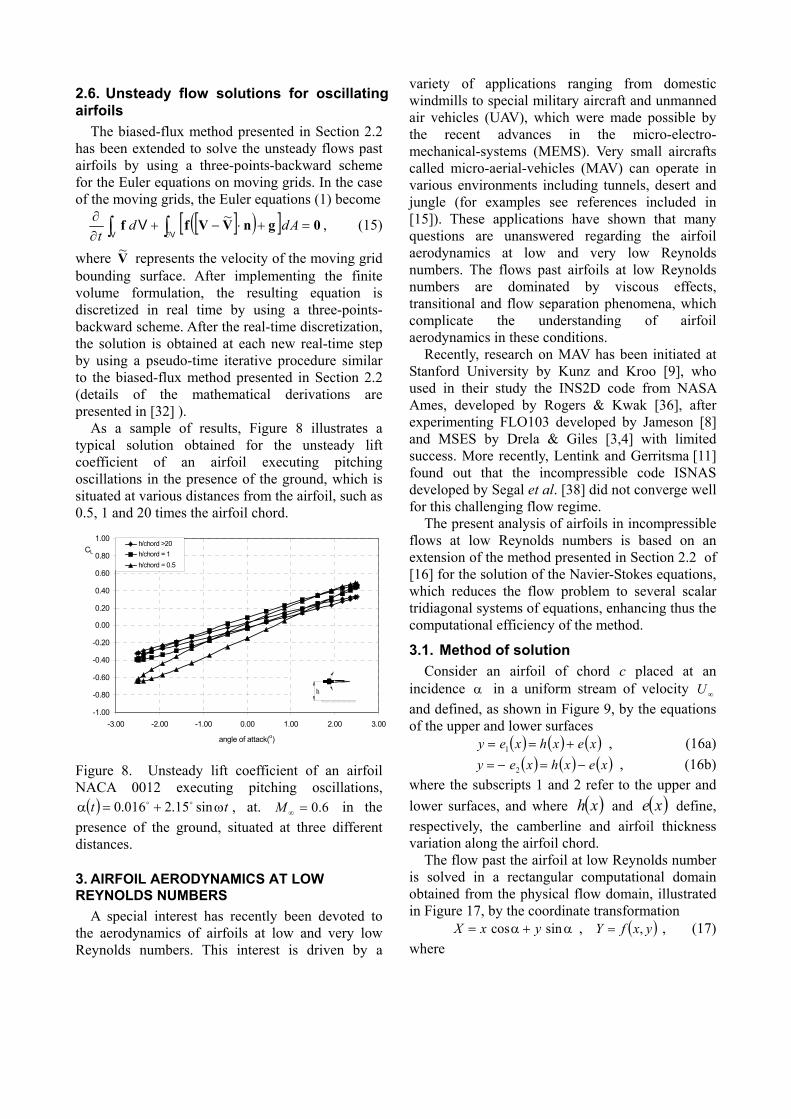
2.6. Unsteady flow solutions for oscillating airfoils

The biased-flux method presented in Section 2.2 has been extended to solve the unsteady flows past airfoils by using a three-points-backward scheme for the Euler equations on moving grids. In the case of the moving grids, the Euler equations (1) become

[ ]( )[ ] 0gnVVff =+⋅−+∂∂

∫∫ ∂VVV Add

t~ , (15)

where represents the velocity of the moving grid bounding surface. After implementing the finite volume formulation, the resulting equation is discretized in real time by using a three-points-backward scheme. After the real-time discretization, the solution is obtained at each new real-time step by using a pseudo-time iterative procedure similar to the biased-flux method presented in Section 2.2 (details of the mathematical derivations are presented in [32] ).

V~

Recently, research on MAV has been initiated at Stanford University by Kunz and Kroo [9], who used in their study the INS2D code from NASA Ames, developed by Rogers & Kwak [36], after experimenting FLO103 developed by Jameson [8] and MSES by Drela & Giles [3,4] with limited success. More recently, Lentink and Gerritsma [11] found out that the incompressible code ISNAS developed by Segal et al. [38] did not converge well for this challenging flow regime.

As a sample of results, Figure 8 illustrates a typical solution obtained for the unsteady lift coefficient of an airfoil executing pitching oscillations in the presence of the ground, which is situated at various distances from the airfoil, such as 0.5, 1 and 20 times the airfoil chord.

The present analysis of airfoils in incompressible flows at low Reynolds numbers is based on an extension of the method presented in Section 2.2 of [16] for the solution of the Navier-Stokes equations, which reduces the flow problem to several scalar tridiagonal systems of equations, enhancing thus the computational efficiency of the method.

-1.00

-0.80

-0.60

-0.40

-0.20

0.00

0.20

0.40

0.60

0.80

1.00

-3.00 -2.00 -1.00 0.00 1.00 2.00 3.00

angle of attack(o)

CLh/chord >20h/chord = 1h/chord = 0.5

h

3.1. Method of solution Consider an airfoil of chord c placed at an

incidence α in a uniform stream of velocity and defined, as shown in Figure 9, by the equations of the upper and lower surfaces

∞U

( ) ( ) (xexhxey +== 1 ) , (16a) ( ) ( ) (xexhxey −=−= 2 ) , (16b) Figure 8. Unsteady lift coefficient of an airfoil

NACA 0012 executing pitching oscillations, , at. in the

presence of the ground, situated at three different distances.

( ) tt ω+=α sin15.2016.0 oo 6.0=∞Mwhere the subscripts 1 and 2 refer to the upper and

lower surfaces, and where and define, respectively, the camberline and airfoil thickness variation along the airfoil chord.

( )xh ( )xe

The flow past the airfoil at low Reynolds number is solved in a rectangular computational domain obtained from the physical flow domain, illustrated in Figure 17, by the coordinate transformation

3. AIRFOIL AERODYNAMICS AT LOW REYNOLDS NUMBERS

A special interest has recently been devoted to the aerodynamics of airfoils at low and very low Reynolds numbers. This interest is driven by a

α+α= sincos yxX , , (17) ( )yxfY ,=where

( )

( )[ ]( )[ ] ( )

( )[ ]( )[ ] ( )

( )

( )⎪⎪⎪⎪⎪⎪

⎩

⎪⎪⎪⎪⎪⎪

⎨

⎧

−<>+−

α+α−+−

−>>+

α+α−+

−<<<α−α−+

α+

><<α+α−−

α−

<<−<α+α−

=

332

32

3131

3

2222

2

1111

1

12

and 1forcossin

and 1forcossin

and10forcossin

cos

and10forcossin

cos

and 0forcossin

,

HyxHH

yxHH

HyxHHH

yxH

xeyxHxexH

xey

xeyxHxexH

xey

HyHxyx

yxf , (18)

solved further using the method presented in Section 2.2 of our paper [16], noting that in this case the length of reference is c instead of H, the reference velocity is instead of , and the coordinate transformation (18) replaces the general transformation (4) from [16].

∞U 0U

in which and , are defined in Figure 9. The upstream inflow and downstream outflow boundaries of the computational domain are defined by and .

α= sin3H 1H 2H

0LX −= α+= cos1LXThe flow past the airfoil at low Reynolds number is

Lower far-field boundary

Upper far-field boundary

α

xc

ycvU∞

uU ∞

V

Xc

Yc

∞U

∞U

1Hc

2Hc

0Lc 1Lc

In-flow boundary

Out-flow boundary

3Hc

( )xhc

( )xec

1c

( )xec 2

( )xec 1

( )xec

Figure 9. Geometry of a cambered airfoil in a uniform flow at incidence.

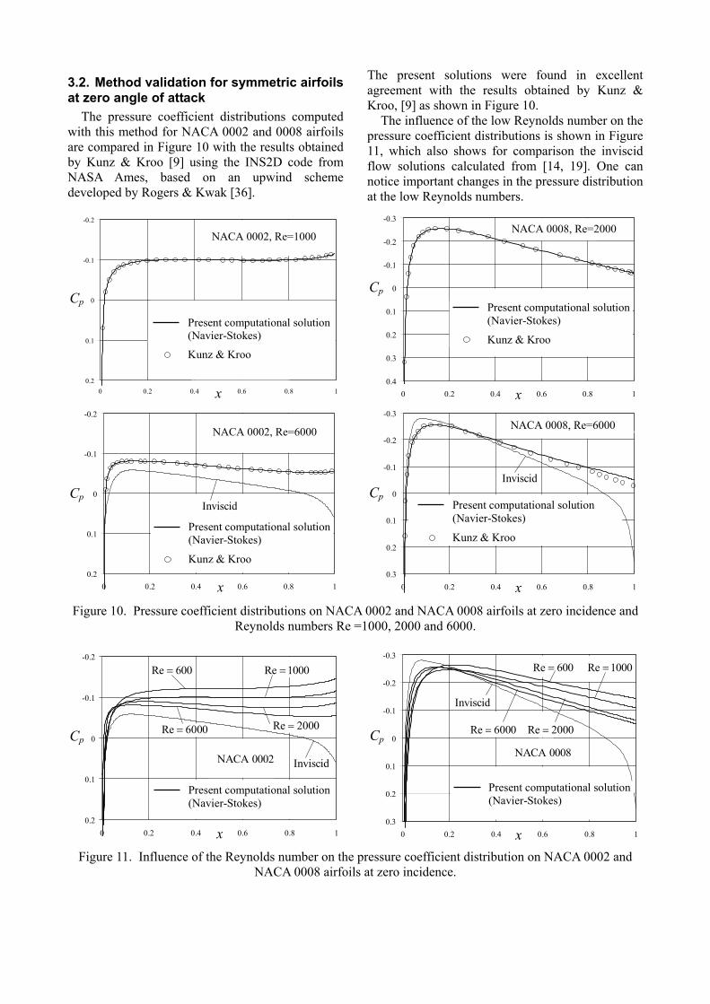
3.2. Method validation for symmetric airfoils at zero angle of attack

The pressure coefficient distributions computed with this method for NACA 0002 and 0008 airfoils are compared in Figure 10 with the results obtained by Kunz & Kroo [9] using the INS2D code from NASA Ames, based on an upwind scheme developed by Rogers & Kwak [36].

The present solutions were found in excellent agreement with the results obtained by Kunz & Kroo, [9] as shown in Figure 10.

The influence of the low Reynolds number on the pressure coefficient distributions is shown in Figure 11, which also shows for comparison the inviscid flow solutions calculated from [14, 19]. One can notice important changes in the pressure distribution at the low Reynolds numbers.

-0.2

-0.1

0

0.1

0.20 0.2 0.4 0.6 0.8 1

Cp

x

NACA 0002, Re=1000

Present computational solution (Navier-Stokes)

Kunz & Kroo

-0.2

-0.1

0

0.1

0.20 0.2 0.4 0.6 0.8 1

Cp

x

Present computational solution (Navier-Stokes)

Kunz & Kroo

NACA 0002, Re=6000

Inviscid

-0.3

-0.2

-0.1

0

0.1

0.2

0.3

0.40 0.2 0.4 0.6 0.8 1

Cp

x

Present computational solution (Navier-Stokes)

Kunz & Kroo

NACA 0008, Re=2000

-0.3

-0.2

-0.1

0

0.1

0.2

0.30 0.2 0.4 0.6 0.8 1

Cp

x

Present computational solution (Navier-Stokes)

Kunz & Kroo

NACA 0008, Re=6000

Inviscid

Figure 10. Pressure coefficient distributions on NACA 0002 and NACA 0008 airfoils at zero incidence and Reynolds numbers Re =1000, 2000 and 6000.

-0.2

-0.1

0

0.1

0.20 0.2 0.4 0.6 0.8 1

Cp

x

Present computational solution (Navier-Stokes)

600Re =

0006Re = 0002Re =

0002NACA

1000Re =

Inviscid

-0.3

-0.2

-0.1

0

0.1

0.2

0.30 0.2 0.4 0.6 0.8 1

Cp

x

1000Re =600Re =

0008NACA

0002Re =0006Re =

Inviscid

Present computational solution (Navier-Stokes)

Figure 11. Influence of the Reynolds number on the pressure coefficient distribution on NACA 0002 and NACA 0008 airfoils at zero incidence.

3.3. Solutions for airfoils at incidence Samples of the present solutions computed for

several symmetric and cambered airfoils at various low Reynolds numbers and angles of attack are shown in Figures 12-21 for the lift, drag and pressure coefficients. These solutions were found in good agreement with available previous results [9].

A detailed study of the flow separation on airfoils at low Reynolds numbers has also been performed for various values of the airfoil relative thickness and camber, maximum camber position, incidence and Reynolds number. Sample of results are shown in Figures 22, 23 and Table 1.

0

0.1

0.2

0.3

0.4

0.5

0.6

0 1 2 3 4 5 6 7 8

Present computational solution (Navier-Stokes)

Kunz & Kroo

LC

α

NACA 0002, Re=1000

0

0.1

0.2

0.3

0.4

0.5

0.6

0 1 2 3 4 5 6

NACA 0002, Re=2000

Present computational solution (Navier-Stokes)

Kunz & Kroo

LC

α

0

0.05

0.1

0.15

0.2

0.25

0.3

0.35

0.4

0 1 2 3 4 5 6 7

Present computational solution (Navier-Stokes)

Kunz & Kroo

LC

α

2000Re 0008,NACA =

Figure 12. Lift coefficient variation for NACA 0002 and 0008 airfoils at Re=1000 and 2000.

0

0.1

0.2

0.3

0.4

0.5

0.6

0.7

0.8

0 1 2 3 4 5 6 7 8

LC

α

NACA 2404 NACA 4404 NACA 6404

Present computational solutions(Navier-Stokes), Re=800

0.1

0.11

0.12

0.13

0.14

0.15

0.16

0.17

0.18

0 1 2 3 4 5 6 7 8α

NACA 2404 NACA 4404 NACA 6404

Present computational solutions(Navier-Stokes), Re=800

DC

0

0.1

0.2

0.3

0.4

0.5

0.6

0.7

0.8

0.11 0.13 0.15 0.17

LC

DC

NACA 2404 NACA 4404 NACA 6404

Present computational solutions(Navier-Stokes), Re=800

Figure 13. Lift, drag and drag polar diagrams for NACA 2404, NACA 4404 and NACA 6404 airfoils

at Re=800.

0

0.1

0.2

0.3

0.4

0.5

0.6

0.7

0.8

0 1 2 3 4 5 6 7 8 9

LC

α

Present computational solution (Navier-Stokes)

Kunz & Kroo

1000Re 4402,NACA =

Figure 14. Lift coefficient variation for NACA 4402 airfoil at Re=1000.

0

0.1

0.2

0.3

0.4

0.5

0.6

0.7

0.8

0.1 0.11 0.12 0.13 0.14

LC Present computational solution (Navier-Stokes)

Kunz & Kroo

1000Re 4402,NACA =

DC

0

0.1

0.2

0.3

0.4

0.5

0.6

0.7

0.8

0.07 0.08 0.09 0.1

LC

Present computational solution (Navier-Stokes)

Kunz & Kroo

DC

2000Re 4402,NACA =

Figure 15. Drag polar for NACA 4402 airfoil at Re=1000 and 2000.

0

0.1

0.2

0.3

0.4

0.5

0.6

0.7

0.8

0.1 0.11 0.12 0.13 0.14 0.15

LC

Present computational solution (Navier-Stokes)

Kunz & Kroo

DC

1000Re 4404,NACA =

Figure 16. Drag polar for NACA 4404 airfoil at Re=1000 and 2000.

0.1

0.12

0.14

0.16

0.18

0.2

0.22

0 1 2 3 4 5 6 7 8

Present computational solutions(Navier-Stokes)

α

DC

4404NACA

Re=400 Re=600

Re=800 Re=1000

0

0.1

0.2

0.3

0.4

0.5

0.6

0.7

0.8

0.1 0.12 0.14 0.16 0.18 0.2 0.22

LC

DC

4404NACA

Present computational solutions(Navier-Stokes)

Re=400 Re=600

Re=800 Re=1000

Figure 17. Drag variation and drag polars for NACA 4404 airfoil at Reynolds numbers Re=400,

600, 800 and 1000.

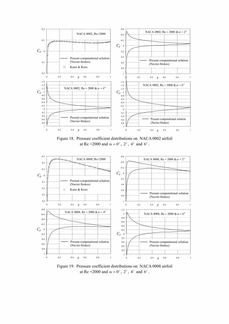
Figure 18. Pressure coefficient distributions on NACA 0002 airfoil at Re =2000 and , , and . o0=α o2 o4 o6

-0.3

-0.2

-0.1

0

0.1

0.2

0.3

0.40 0.2 0.4 0.6 0.8 1

Cp

x

Present computational solution (Navier-Stokes)

Kunz & Kroo

NACA 0008, Re=2000-0.6

-0.4

-0.2

0

0.2

0.4

0.6

0.8

10 0.2 0.4 0.6 0.8 1

Cp

x

Present computational solution (Navier-Stokes)

o2 & 2000Re 0008,NACA == α

-0.8

-0.6

-0.4

-0.2

0

0.2

0.4

0.6

0.8

10 0.2 0.4 0.6 0.8 1

Cp

x

Present computational solution (Navier-Stokes)

o4 & 2000Re 0008,NACA == α-1.2

-1

-0.8

-0.6

-0.4

-0.2

0

0.2

0.4

0.6

0.8

10 0.2 0.4 0.6 0.8 1

Cp

x

Present computational solution (Navier-Stokes)

o6 & 2000Re 0008,NACA == α

-0.2

-0.1

0

0.1

0.20 0.2 0.4 0.6 0.8 1 x

Cp Present computational solution (Navier-Stokes)

Kunz & Kroo

NACA 0002, Re=2000-0.6

-0.4

-0.2

0

0.2

0.4

0.6

0.8

10 0.2 0.4 0.6 0.8 1

Cp

x

Present computational solution (Navier-Stokes)

o2 & 2000Re 0002,NACA == α

-1.6-1.4-1.2

-1-0.8-0.6-0.4-0.2

00.20.40.60.8

10 0.2 0.4 0.6 0.8 1

Cp

x

Present computational solution (Navier-Stokes)

o4 & 2000Re 0002,NACA == α

-1.6-1.4-1.2

-1-0.8-0.6-0.4-0.2

00.20.40.60.8

10 0.2 0.4 0.6 0.8 1

Cp

x

Present computational solution (Navier-Stokes)

o6 & 2000Re 0002,NACA == α

Figure 19. Pressure coefficient distributions on NACA 0008 airfoil at Re =2000 and o , o , o and o6 . 0=α 2 4

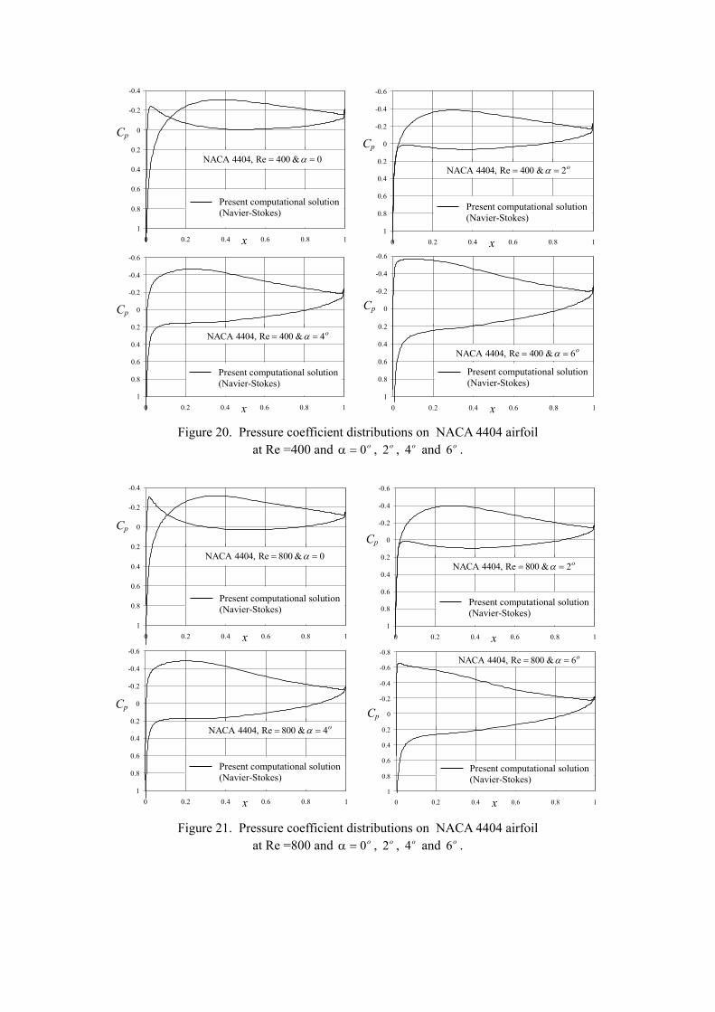
Figure 20. Pressure coefficient distributions on NACA 4404 airfoil at Re =400 and , , and . o0=α o2 o4 o6

-0.4

-0.2

0

0.2

0.4

0.6

0.8

10 0.2 0.4 0.6 0.8 1

Cp

x

Present computational solution (Navier-Stokes)

0& 008Re 4404,NACA == α

-0.6

-0.4

-0.2

0

0.2

0.4

0.6

0.8

10 0.2 0.4 0.6 0.8 1

Cp

x

Present computational solution (Navier-Stokes)

o2 & 800Re 4404,NACA == α

-0.6

-0.4

-0.2

0

0.2

0.4

0.6

0.8

10 0.2 0.4 0.6 0.8 1

Cp

x

Present computational solution (Navier-Stokes)

o4 & 800Re 4404,NACA == α

-0.8

-0.6

-0.4

-0.2

0

0.2

0.4

0.6

0.8

10 0.2 0.4 0.6 0.8 1

Cp

x

o6 & 800Re 4404,NACA == α

Present computational solution (Navier-Stokes)

-0.4

-0.2

0

0.2

0.4

0.6

0.8

10 0.2 0.4 0.6 0.8 1

Cp

x

Present computational solution (Navier-Stokes)

0& 004Re 4404,NACA == α

-0.6

-0.4

-0.2

0

0.2

0.4

0.6

0.8

10 0.2 0.4 0.6 0.8 1

Cp

x

o2 & 400Re 4404,NACA == α

Present computational solution (Navier-Stokes)

-0.6

-0.4

-0.2

0

0.2

0.4

0.6

0.8

10 0.2 0.4 0.6 0.8 1

Cp

x

Present computational solution (Navier-Stokes)

o6 & 400Re 4404,NACA == α

-0.6

-0.4

-0.2

0

0.2

0.4

0.6

0.8

10 0.2 0.4 0.6 0.8 1

Cp

x

Present computational solution (Navier-Stokes)

o4 & 400Re 4404,NACA == α

Figure 21. Pressure coefficient distributions on NACA 4404 airfoil at Re =800 and o , o , o and o . 0=α 2 4 6

Table 1. Flow separation comparison for symmetric NACA airfoils at Re=2000 and . o6=α

Airfoil type Separation position, sx Reattachment position, rx Separation length, sl

NACA 0002 0.009448 0.983755 0.974307

NACA 0004 0.345298 0.985038 0.639739

NACA 0006 0.493517 0.987267 0.493749

NACA 0008 0.501505 0.986959 0.485453

x

y

0.8 0.9 1

-0.1

-0.05

0

0.05

0.1

x

y

0.8 0.9 1

-0.1

-0.05

0

0.05

0.1

x

y

0.8 0.9 1

-0.1

-0.05

0

0.05

0.1

Figure 22. Streamline contours for NACA 0004 airfoil at Re=2000 and , and. . o4=α o6 o7

x

y

0.6 0.7 0.8 0.9 1

-0.1

0

0.1

0.2

x

y

0.6 0.7 0.8 0.9 1

-0.1

0

0.1

0.2

x

y

0.6 0.7 0.8 0.9 1

-0.1

0

0.1

0.2

x

y

0.6 0.7 0.8 0.9 1

-0.1

0

0.1

0.2

Figure 23. Influence of Reynolds number: Streamline contours for NACA 4404 airfoil at and Reynolds numbers Re=400, 600, 800 and 1000, respectively.

o8=α

4. CONCLUSIONS The paper presents efficient solutions of the Euler and Navier-Stokes equations based on finite difference and finite volume formulations.

A biased-flux method using an explicit finite volume formulation is first presented for the solution of the Euler equations. A second-order scheme is used for the flux calculation, with an upwind or downwind bias for the flow variables, according to the subsonic or supersonic character of the local flow. This method avoids thus the odd-and-even-points decoupling, which is present in other methods, and as a result, does not require an added artificial-dissipation, displaying a very good computational efficiency in all problems studied. Validated for compressible flows with expansions and shock waves in nozzles, this method is then used to obtain solutions for subsonic, transonic and supersonic flows past airfoils.

Efficient Navier-Stokes solutions are also presented for the viscous flows past airfoils at low Reynolds numbers. These solutions are obtained in a rectangular computational domain, defined by a coordinate transformation, with a method using artificial compressibility and a finite difference formulation on a stretched staggered grid. As a result of the coordinate transformation, there is no need for a complex grid generation procedure. The computational efficiency of this method is very good due to a special decoupling procedure of the momentum equations, with the aid of the continuity equation augmented by artificial compressibility, which finally reduces the flow problem to the efficient solution of scalar tridiagonal systems.

This method has been successfully validated by comparison with previous available results, obtained by Kunz and Kroo, for the lift, drag and pressure coefficients for Reynolds numbers between 1000 and 6000. Then the method has been used to obtain solutions at lower Reynolds numbers between 400 and 800, for which there are no previous results. A detailed analysis of the flow separations on airfoils at low Reynolds number has also been performed with this method.

REFERENCES 1. Anderson W.K., Thomas J.L., VanLeer B.

(1986) Comparison of finite volume flux vector splittings for the Euler equations. AIAA Journal 24:1453-1460

2. Chorin A. (1967) A numerical method for solving incompressible viscous flow problems. Journal of Computational Physics 2: 12-26

3. Drela M., Giles M.B. (1987) Viscous-Inviscid analysis of transonic and low Reynolds number airfoils. AIAA Journal 25: 1347-1355

4. Drela M., Giles, M.B. (1987) ISES- A Two-Dimensional Viscous Aerodynamic Design and Analysis Code. AIAA Paper 87-0424

5. Eidelman S., Colella P., Shreeve R.P. (1984) Application of the Godunov method and its second-order extension to cascade flow modeling. AIAA Journal 22:1609-1615

6. Godunov S.K. (1959) Finite difference method for numerical computation of discontinuous solutions of the equations of fluid dynamics. Math Sb 47:271-306

7. Huteau T., Lee T., Mateescu D. (2000) Flow past a 2-D backward-facing step with an oscillating wall. Journal of Fluids and Structures 14: 691-696

8. Jameson A., Schmidt W., Turkel E. (1981) Numerical Solution of the Euler Equations by Finite Volume Methods Using Runge-Kutta Time Stepping Schemes. AIAA Paper 81-1259

9. Kunz P., Kroo I. (2000) Analysis and design of airfoils for use at ultra-low Reynolds numbers. Proceedings of the AIAA Fixed, Flapping and Rotating Wing Aerodynamics at Very Low Reynolds Numbers Conference. Notre Dame, June 5-7, pp. 35-60

10. Lee T., Mateescu D. (1998) Experimental and numerical investigations of 2-D backward-facing step flow. Journal of Fluids and Structures 12:703-716

11. Lentink D., Gerritsma M. (2003) Influence of airfoil shape on performance in insect flight. AIAA Paper 2003-3447, June 23-26

12. MacCormack R.W., Rizzi A.W., Inouye M. (1976) Steady supersonic flowfields with embedded subsonic regions. Computational methods and problems in aeronautical fluid dynamics, Academic Press, pp 424-447

13. Mateescu D., Abdo M. (2005) Low-Reynolds number aerodynamics of airfoils at incidence. Applied Aerodynamics Conference, 43rd AIAA Aerospace Sciences Meeting, Reno, Nevada, AIAA Paper 2005-1038, pp. 1-12.

14. Mateescu D., Abdo M. (2004) Efficient second-order analytical solutions for airfoils in subsonic flows. Aerospace Science and Technology Journal (accepted for publication)

15. Mateescu D., Abdo M. (2004) Aerodynamic analysis of airfoils at very low Reynolds numbers. Applied Aerodynamics Conference, 42nd AIAA Aerospace Sciences Meeting, Reno, Nevada, AIAA Paper 2004-1053, pp. 1-11

16. Mateescu D. (2004) Efficient methods for 2D and 3D steady and unsteady confined flows based on the solution of the Navier-Stokes equations. Proceedings of the 6th International Conference on Hydraulic Machinery and Hydrodynamics. Timisoara, Romania.

17. Mateescu D. (2004) Solutions of the Euler and Navier-Stokes equations using Lagrangian and spectral formulations. (in preparation)

18. Mateescu D. (2003) Analysis of aerodynamic problems with geometrically unspecified boundaries using an enhanced Lagrangian method. Journal of Fluids and Structures 17: 603-626

19. Mateescu D., Abdo M. (2003) Nonlinear theoretical solutions for airfoil aerodynamics. 21st Applied Aerodynamics Conference, Orlando, Florida, AIAA Paper 2003-4296, pp. 1-16.

20. Mateescu D., Venditti D. (2001) Unsteady confined viscous flows with oscillating walls and multiple separation regions over a downstream-facing step. Journal of Fluids and Structures 15: 1187-1205

21. Mateescu D., Venditti D. (2000) Analysis of unsteady confined viscous flows with separation regions for fluid-structure interaction problems. Proceedings of the 7th International Conference on Flow-Induced Vibrations, Luzern, Switzerland, pp. 327-334

22. Mateescu D., Mekanik A., Païdoussis M.P. (1996) Analysis of 2-D and 3-D unsteady annular flows with oscillating boundaries based on a time-dependent coordinate transformation. Journal of Fluids and Structures 10: 57-77

23. Mateescu D., Pottier T., Perotin L., Granger S. (1995) Three-dimensional unsteady flows between oscillating eccentric cylinders by an enhanced hybrid spectral method. Journal of Fluids and Structures 9: 671-695

24. Mateescu D., Stanescu D. (1995) A biased flux method for solving the Euler equations in subsonic, transonic and supersonic flows. Computational Methods and Experimental Measurements VII. Computational Mechanics Public. Southampton and Boston, pp. 327-335

25. Mateescu D., Païdoussis M.P., Bélanger F. (1994) A time-integration method using artificial compressibility for unsteady viscous flows. Journal of Sound and Vibration 177: 197-205

26. Mateescu D., Païdoussis M.P., Bélanger F. (1994) Unsteady annular viscous flows between oscillating cylinders. Part I: Computational solutions based on a time integration method. Journal of Fluids and Structures 8: 489-507

27. Mateescu D., Païdoussis M.P., Bélanger F. (1994) Unsteady annular viscous flows between oscillating cylinders. Part II: A hybrid time-integration solution based on azimuthal Fourier expansions for configurations with annular backsteps. Journal of Fluids and Structures 8: 509-527

28. Mateescu D., Païdoussis M.P., Sim W.G. (1994) A spectral collocation method for confined unsteady flows with oscillating boundaries. Journal of Fluids and Structures 8: 157-181

29. Mateescu D., Païdoussis M.P., Bélanger F. (1989) A theoretical model compared with experiments for the unsteady pressure on an cylinder oscillating in turbulent annular flow. Journal of Sound and Vibration 135: 487-498

30. Mateescu D., Lauzon M. (1989) An explicit Euler method for internal flow computation. Computers and experiments in fluid flow, G.M. Carlomagno and C.A. Brebbia, Springer-Verlag, Berlin, pp 41-50

31. Mateescu D., Païdoussis M.P., Bélanger F. (1988) Unsteady pressure measurements on an oscillating cylinder in narrow annular flow. Journal of Fluids and Structures 2: 615-628

32. Mateescu D., Ming L. (2004) Analysis of aerodynamic interactions based on the solution of the Euler equations. (in preparation)

33. Ni R.H. (1982) A multiple-grid scheme for solving the Euler equations. AIAA Journal 20: 1565-1570

34. Raney D.L., Waszak M.R. (2003) Biologically inspired micro-flight research. AIAA Paper 2003-01-3042

35. Roe P.L. (1986) Discrete models for the numerical analysis of time-dependent multidimensional gas dynamics. J Comp Physics 63:458-476

36. Rogers S., Kwak D. (1990) An upwind differencing scheme for the time-accurate incompressible Navier-Stokes equations. AIAA Journal 28: 253-262

37. Schmidt W., Jameson A. (1985) Euler solver as an analysis tool for aircraft aerodynamics. Recent advances in numerical methods in fluids. Swansea, Wales pp 371-404

38. Segal G., Zijlema M., Nooyen R.V., Moulinec C. (2001) User Manual of the Delft incompressible flow solver. Delft University of Technology, version 1.1

39. Thiber J., Grandjacques M., Ohman L. (1979) Experimental data base for computer program assessment – NACA 0012 airfoil. Report of Fluid Dynamics Panel, AGARD-AR-138, pp. A1-36