General rights Copyright and moral rights for the publications made accessible in the public portal are retained by the authors and/or other copyright owners and it is a condition of accessing publications that users recognise and abide by the legal requirements associated with these rights.

• Users may download and print one copy of any publication from the public portal for the purpose of private study or research. • You may not further distribute the material or use it for any profit-making activity or commercial gain • You may freely distribute the URL identifying the publication in the public portal

If you believe that this document breaches copyright please contact us providing details, and we will remove access to the work immediately and investigate your claim.

Downloaded from orbit.dtu.dk on: May 20, 2018

Efficient Estimation of Extreme Non-linear Roll Motions using the First-order ReliabilityMethod (FORM)

Jensen, Jørgen Juncher

Published in:Marine Science and Technology

Link to article, DOI:10.1007/s00773-007-0243-z

Publication date:2007

Document VersionPublisher's PDF, also known as Version of record

Link back to DTU Orbit

Citation (APA):Jensen, J. J. (2007). Efficient Estimation of Extreme Non-linear Roll Motions using the First-order ReliabilityMethod (FORM). Marine Science and Technology, 12(4), 191-202. DOI: 10.1007/s00773-007-0243-z

1 3

ORIGINAL ARTICLE

J Mar Sci Technol (2007) 12:191–202DOI 10.1007/s00773-007-0243-z

J.J. Jensen (*)Department of Mechanical Engineering, Technical University of Denmark, Nils Koppel Allé, Building 403/024, Kgs. Lyngby, DK 2800, Denmarke-mail: jjj@mek.dtu.dk

Effi cient estimation of extreme non-linear roll motions using the fi rst-order reliability method (FORM)

Jørgen Juncher Jensen

Key words Roll motion · Parametric roll · FORM · Reliability · Mean out-crossing rate · On-board decision support systems

1 Introduction

The roll motion of ships can lead to various types of failures, ranging from seasickness, cargo shift, and loss of containers to capsize of the vessel. Hence, it is impor-tant to minimise the roll motion during a voyage. Cur-rently, on-board decision support systems, e.g., those described by Rathje1 and Nielsen et al.,2 are being installed in vessels with the aim of providing the offi cer on watch with guidance on the best possible route, taking into account the weather forecast, the time constraints for the voyage, and the limiting criteria for motions, accelerations, and loads.

A major problem is real-time estimation of the sea state. Here, two approaches are tested in full-scale sce-narios. The fi rst is based on the use of a wave radar, e.g., the WAVEX system (Borge et al.3), and the second uses ship responses (e.g., motions, accelerations, and strains) measured in real time by sensors installed on board together with linear transfer functions to estimate the sea state, see the work of Nielsen,4 in which a comparison between the two approaches is also found.

After estimation of the sea state, a real-time estima-tion of the maximum ship responses within the next few hours as a function of ship speed and course is needed to guide the offi cer on the action to take if excessive responses are foreseen with the present course and speed. For linear responses, the standard frequency domain approach using transfer functions can easily be applied. For non-linear responses, time domain simulations are

Received: August 29, 2006 / Accepted: February 16, 2007© JASNAOE 2007

Abstract In on-board decision support systems, effi cient procedures are needed for real-time estimation of the maximum ship responses to be expected within the next few hours, given online information on the sea state and user-defi ned ranges of possible headings and speeds. For linear responses, standard frequency domain methods can be applied. For non-linear responses, as exhibited by the roll motion, standard methods such as direct time domain simulations are not feasible due to the required computational time. However, the statistical distribu-tion of non-linear ship responses can be estimated very accurately using the fi rst-order reliability method (FORM), which is well known from structural reliability problems. To illustrate the proposed procedure, the roll motion was modelled by a simplifi ed non-linear proce-dure taking into account non-linear hydrodynamic damping, time-varying restoring and wave excitation moments, and the heave acceleration. Resonance excita-tion, parametric roll, and forced roll were all included in the model, albeit with some simplifi cations. The result is the mean out-crossing rate of the roll angle together with the most probable wave scenarios (critical wave epi-sodes), leading to user-specifi ed specifi c maximum roll angles. The procedure is computationally very effective and can thus be applied to real-time determination of ship-specifi c combinations of heading and speed to be avoided in the actual sea state.

1 3

192 J Mar Sci Technol (2007) 12:191–202

often performed to obtain short-term statistics for the non-linear roll response of ships, e.g., see the work of Krüger et al.5 and Daalen et al.6 However, less time-consuming stochastic procedures have also been sug-gested. Most of these procedures are based on simplifying, but often reasonable, assumptions such as equivalent linear damping (Bulian and Francescutto7), second- or third-order perturbation procedures (Neves and Rodri-guez8), Melnikov functions (Hsieh at al.9 and Spyrou10), and moment closure techniques (Ness et al.11).

In the present study, the fi rst-order reliability method (FORM) was applied instead and was shown to be an accurate and effi cient procedure for estimation of the extreme value statistics of even very non-linear responses such as parametric rolling. The advantage of the present procedure is that assumptions in the physical model are not needed, as full three-dimensional non-linear hydro-dynamic codes can be applied within the FORM analy-sis. Furthermore, in contrast to Monte Carlo simulations, the calculation time in the FORM analysis does not depend very much on the exceedance level considered and thus even very rare events can be predicted within a short calculation time.

A problem related to on-board decision support systems is the estimation of limit state parameters for the ship. This involves a discussion of the various hazards: seasickness, destruction of sensible equipment, cargo shift, loss of containers, and, ultimately, the capsizing or sinking of the vessel. Clearly, both a model for the failure mode and a cost model for the consequences are needed to defi ne a proper limiting value to be presented to the offi cer on watch. A general procedure based on a so-called utility function has been suggested by Søborg and Friis-Hansen.12 In the present work, a simplifi ed model for the roll motion was used to calculate only the exceed-ance level of specifi c roll angles. Thus, no attempt to formulate a realistic limiting roll angle or to defi ne a suitable utility function was made. It should, however, be mentioned that such limit state parameters and crite-ria were included in the SAFEDOR project, see the Acknowledgment, and can easily be implemented in the present FORM approach.

2 First-order reliability method applied to wave loads

2.1 Design point and reliability index

In FORM analysis, the excitation or input process is a stationary stochastic process. Considering wave loads on marine structures in general, the input process is the wave elevation and the associated wave kinematics. For moderate sea states, the wave elevation can be consid-

ered as Gaussian distributed, whereas for severer wave conditions, corrections for non-linearities must be incor-porated. Such corrections are discussed and accounted for by using a second-order wave theory in a FORM analysis of a jack-up platform (Jensen and Capul13). In the present work with the roll motion of a ship, linear, long-crested waves are assumed and hence the normal distributed wave elevation H(X, t) as a function of space X and time t can be written:

H X t u c X t u c X ti i i ii

n

, , ,( ) = ( ) + ( )( )=∑

1 (1)

where the variables ui, ui are uncorrelated, standard nor-mally distributed variables to be determined by the sto-chastic procedure and with the deterministic coeffi cients given by:

c x t t k X

c x t t k X

S d

i i i i

i i i i

i i i

,

,

( ) = −( )( ) = − −( )

= ( )

σ ωσ ω

σ ω ω

cos

sin2

(2)

where wi, ki = w2i /g are the n discrete frequencies and wave

numbers applied. Furthermore, S(w) is the wave spec-trum and dwi the increment between the discrete frequen-cies. It is easily seen that the expected value E[H2] = ∫S(w)dw, thus the wave energy in a stationary sea is pre-served. Short-crested waves could be incorporated, if needed, but require more unknown variables ui, ui.

From the wave elevation (Eqs. 1 and 2) and the asso-ciated wave kinematics, any non-linear wave-induced response f(t) of a marine structure can in principle be determined by a time domain analysis using a proper hydrodynamic model:

φ φ= ( )t u u u u u un n1 1 2 2, , , , , , initial conditions, . . . (3)

Each of these realisations represents the response for a possible wave scenario. The infl uence of the initial condi-tions should be eliminated as stationary stochastic responses are considered. The realisation which exceeds a given threshold f0 at time t = t0 with the highest prob-ability is sought. This problem can be formulated as a limit state problem, which is well known within time-invariant reliability theory (Der Kiureghian14):

G u u u u u u

t u u u u u un n

n n

1 1 2 2

0 0 1 1 2 2 0

, , , , , ,

, , , , , ,

. . .

. . .

( )≡ − ( ) =φ φ (4)

The integration in Eq. 4 must cover a suffi cient time period {0, t0} to avoid any infl uence on f (t0) of the initial conditions at t = 0, i.e., the integration period must be longer than the memory in the system. Proper values of

1 3

J Mar Sci Technol (2007) 12:191–202 193

t0 would usually be 1–3 min, depending on the damping in the system. Hence, to avoid repetition in the wave system and for accurate representation of typical wave spectra, n = 15–50 is suitable.

An approximate solution can be obtained using FORM. The limit state surface G is given in terms of the uncorrelated standard normally distributed variables {ui, ui}, and hence determination of the design point {u*i , u*i }, defi ned as the point on the failure surface G = 0 with the shortest distance to the origin, is rather straightfor-ward. A linearization around this point replaces Eq. 4 with a hyperplane in 2n space. The distance bFORM

βFORM i ii

n

u u= +( )=∑min 2 2

1 (5)

from the hyperplane to the origin is denoted the FORM reliability index. The calculation of the design point {u*i , u*i } and the associated value of bFORM can be performed by standard reliability codes (e.g., that of Det Norske Veritas15). Alternatively, standard optimisation codes using Eq. 5 as the objective function and Eq. 4 as the constraint can be applied.

The deterministic wave profi le

H X t u c X t u c X ti i i ii

n

* , * , * ,( ) = ( ) + ( )( )=∑

1 (6)

can be considered as a design wave or a critical wave episode. It is the wave scenario with the highest proba-bility of occurrence that leads to the exceedance of the specifi ed response level f0. For linear systems, the result reduces to the standard Slepian model, see e.g., Lind-gren,16 Tromans et al.,17Adegeest et al.,18 and Dietz et al.19 The critical wave episode is a useful result as it can be used as input in more elaborate time domain simulations to correct for assumptions made in the hydrodynamic code, Eq. 3, applied in the FORM calculations. Such a model-correction-factor approach provides an effective tool for accounting for even very complicated non-linear effects (Ditlevsen and Arnbjerg-Nielsen20).

It should be noted that other defi nitions of design waves based on a suitable non-uniform distribution of phase angles have been applied, especially for experi-mental application in model basins. The selection of the phase angle distribution is, however, not obvious, see e.g., Alford et al.21

2.2 Mean out-crossing rates and exceedance probabilities

The time-invariant peak distribution follows from the mean out-crossing rates. Within a FORM approxima-tion, the mean out-crossing rate can be written as follows (see Jensen and Capul13):

ν φπβ

ωβ

( )0

12 2 2 2

1

12

2

= +( )−

=∑

FORMi i i

i

n

e u uFORM * *

(7)

This is based on a general formula given by Koo et al.22 Thus, the mean out-crossing rate is expressed analyti-cally in terms of the design point and the reliability index. For linear processes, it reduces to the standard Rayleigh distribution. Often, the gradient vector {a*i , α*i } = {u*i , u*i }/bFORM to the design point does not vary much with exceedance level f0. Hence, Eq. 7 reduces to:

ν φ νβ

( )0 0

12

2

=−

e FORM

(8)

where n0 can be viewed as an effective mean zero out-crossing rate. Finally, on the assumption of statistically independent peaks and, hence, a Poisson distributed process, the probability of exceedance of the level f0 in a given time T can be calculated from the mean out-crossing rate n(f0):

P eT

Tmax ( )φ φ ν φ>

= − −

0 1 0

(9)

The present procedure can be considered as an alterna-tive to the random constrained simulation, e.g., see Dietz et al.19 The present method has, however, the advantage that the number of time domain simulations is much smaller due to the very effi cient optimisation procedures within FORM; in addition, it does not require the curve-fi tting of lines of constant probabilities needed in the other procedure. Furthermore, the FORM procedure does not rely on a mean wave conditional on a linear response and can hence be applied also to bifurcation types of problems such as parametric roll. In such cases, the optimisation procedure used in the FORM analysis must be chosen appropriately, i.e., it must be of the non-gradient type. In the present case, a circle step approach is used, see Det Norske Veritas.15 In this approach, a circle is drawn in u-space and the point with the lowest value of G is determined. Then the intersection between the line through origin and this point and G = 0 is found. In the next iteration, a new circle in drawn through this intersection point and so on. Furthermore, to facilitate the convergence of the optimisation procedure, the limit

1 3

194 J Mar Sci Technol (2007) 12:191–202

state surface, Eq. 4, is replaced by a logarithm transformation:

�G u u u u u u

t u u u un n( . . . )

) ( . .1 1 2 2

0 0 1 1 2 2

, , , , , ,

logt( logt( , , , ,≡ −φ φ .. ))

)

log( );

;

log( );

, ,

logt(

u u

y

y y

y y

y y

n n =

≡− − − < −

− ≤ ≤+ <

0

1 1

1 1

1 1

(10)

FORM is signifi cantly faster than direct Monte Carlo simulations, and most often is very accurate. In a study (Jensen and Pedersen23) dealing exclusively with the parametric rolling of ships in head seas, the FORM approach was found to be two orders of magnitude faster than direct simulation for realistic exceedance levels and with results deviating by less than 0.1 in the reliability index. Similar observations were noted in the present study.

It should be mentioned that the present procedure bears some resemblance to the approach adopted by Søborg and Friis-Hansen.12 The difference is basically in the excitation process, where the present continuous wave excitation in Søborg and Friis-Hansen12 is replaced by a discrete excitation in time. The advantage of the present procedure is that it can directly represent the shape of actual wave spectra and that it provides an analytical formula, Eq. 7, for the mean out-crossing rate.

3 Roll motion of a ship

A very comprehensive discussion of intact stability can be found in a recent ITTC report on ship stability in waves, ITTC.24 The report discusses various modes of failure, e.g., capsize, and the prediction procedures available. The report is partly based on the result of a questionnaire distributed to a large number of organisa-tions and thus refl ects very well the current status. To cover all modes of failure (static loss of stability, para-metric excitation, dynamic rolling, resonance excitation, and broaching) a general, non-linear, six-degrees-of-freedom time domain procedure, including viscous effects and manoeuvring models, is probably needed. Some codes, e.g., LAMP (France et al.25 and Shin et al.26), seem to be able to achieve this with reasonable accuracy, but are very time-consuming to run, restricting the application to regular waves or very short stochastic realisations.

Other procedures have more limited capabilities as some of the capsize modes are excluded. An example is the ROLLS procedure (Kroeger27), in which the follow-

ing non-linear differential equation is used to estimate the roll angle f(t), omitting the terms due to wind and fl uids in tanks:

( sin cos )

( ) ( )

I I M M M

g w GZ I

xx xz sy d

xz

− +( ) + −

− − − +

=ψ φ θ φ

φ θ θ

φ φ��

�� ��∆ ��

�� �φ φ

ψ ψφ φ

2

2

( )− +( )

sin

cos

(11)

Here, Mf, Msy, and Md are the roll moments due to waves, sway and yaw, and hydrodynamic damping, respectively. Furthermore, Ixx and Ixz are the mass moment of inertia about the longitudinal axis and the cross-term mass moment of inertia. The coordinate system is situated with the origin at the centre of gravity. The displacement of the ship is denoted by ∆, and g is the acceleration of gravity. The instantaneous value of the righting arm, GZ, in irregular waves is calculated approximately using the so-called Grim’s effective wave. The heave w, pitch q, and yaw y motions are determined by standard strip theory formulations, whereas the surge motion is calculated from the incident wave pressure distribution. The advantage of this formulation com-pared to full non-linear calculations is the much faster computational speed, while still retaining a coupling between all six degrees of freedom, see Krüger et al.5 The model, however, cannot deal with broaching.

In the present procedure, both the heave motion w and the wave-induced roll moment Mf are taken to be linear functions of the wave elevation. The cross-term mass moment of inertia is assumed to be small, and pitch is thus only included through the static balancing of the vessel in waves in the calculation of the GZ curve. Fur-thermore, the sway, yaw, and surge motions are ignored because the vertical motions have the largest infl uence on the instantaneous GZ curve. The damping term Md is modelled by a standard combination of a linear, a quadratic, and a cubic variation in the roll velocity. With these simplifi cations, Eq. 11 becomes:

�� � � �� ��

φ β ω φ β φ φ β φω

φφ

φ

φ= − − − − −( ) +2 1 23

3

2

g w GZr

M

Ix xx

( )

(12)

where rx is the roll radius of gyration. The roll frequency wf is given by the metacentric height GMsw in still water:

ωφ = gGMr

sw

x (13)

It is clear that this model is very simplistic, but it is well suited to illustrate the proposed stochastic procedure as it can model parametric rolling, resonance excitation, and forced rolling. Hence, it is possible to identify which

1 3

J Mar Sci Technol (2007) 12:191–202 195

mode is the most probable for a given combination of sea state, speed, and heading. As broaching and dynamic rolling (where a strong coupling to surge exists) cannot be modelled by Eq. 12, following and stern quartering seas will be excluded from the calculations, and heading angles y in the range 60°–180° (head sea) only will be considered.

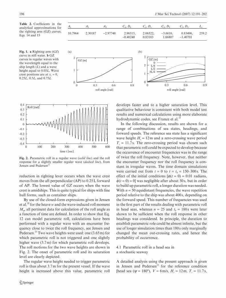
The instantaneous GZ curve in irregular waves was estimated from numerical results for a regular wave with a wavelength equal to the length L of the vessel and a wave height equal to 0.05 L. These numerical results were fi tted with analytical approximations of the form:

GZ x C C C Cx

L

D D

cc

e

( ) sin cos

sin

φ φ φ φ φ π

φ φ

, = + + +( )

+ + +

0 1 33

55 4

0 1 DD Dx

Lc

e3

35

5φ φ π+( )

sin (14)

where the wave crest position xc is measured relative to the aft end of the vessel. Similarly, the GZ curve in still water was fi tted by:

GZ GM A A A Asw sw( ) sinφ φ φ φ φ= −( ) + + +1 1 33

55

(15)

The coeffi cients (A1, A3, A5, C0, C1, C3, C5, D0, D1, D3, D5, Le) in Eqs. 14 and 15 were found by the least-squares method. Other polynomial or Fourier series representa-tions have been suggested, e.g., those of Spyrou10 and Bulian,29 and generally a very good fi t can be achieved for the range of roll angles of interest.

In a stochastic seaway, the following approximation of the instantaneous value of the righting arm GZ(t) is then applied:

GZ t GZh t

LGZ x t GZsw c sw( ) ( )

( ).

( )φ φ φ φ, ,= + ( ) − ( )( )0 05

(16)

This linear relation between GZ and h is clearly an assumption that needs validation. It is used here for the sake of simplicity, but also because the model given in Eq. 12 by itself gives only an approximate description of reality.

The instantaneous wave height h(t) along the length of the vessel and the position of the crest xc are deter-

mined by an equivalent wave procedure somewhat similar to the one used by Kroeger27:

a tL

H X x t tx

Ldx

b tL

H X x t t

e

L

e

e

e

( ) cos

( )

= ( )( )

= ( )( )

∫2 2

2

0

, ,

, ,

π

00

2 2

2

2

L

e

c

e xL

dx

X x t x Vt

h t a t b t

x

∫

( ) = +( )= +

sin

cos

( ) ( ) ( )

(

π

ψ,

tt

L a th t

b t

LL a t

h t

e

ee

)

( )( )

( )

( )(

=

>

−

22

0

22

π

π

arccos if

arccos))

( )

<

if b t 0

(17)

Note than in beam seas, h(t) = 0 such that GZ(f,t) = GZsw(f). Stationary sea conditions were assumed and were specifi ed by a JONSWAP wave spectrum with sig-nifi cant wave height Hs and zero-crossing period Tz. The frequency range was taken to be p ≤ wTz ≤ 3p, covering the main part of the JONSWAP spectrum.

Solutions were obtained by embedding the time domain simulation routine, Eq. 12, in a standard FORM code. In the present case, the software PROBAN (Det Norske Veritas15) was used. In the following, results for a container ship are presented and discussed.

4 Numerical example

A container ship with main particulars given in Table 1 is considered. The damping coeffi cients, b1–b3, are taken, quite arbitrarily, from a study considering a different vessel (Bulian29), but correspond to about 0.05 in equiva-lent linear damping. The speed is chosen such that the mean encounter frequency is close to twice the roll natural frequency. The coeffi cients in Eqs. 14 and 15 are given in Table 2.

The units of the coeffi cients are metres with the roll angle given in radians. The approximations are accurate for roll angles up to 0.9 radians, see Jensen and Olsen.28 It is noted that the optimal value of the parameter Le is slightly shorter than the length of the ship L. The GZ curves are shown in Fig. 1 and it is clear that a signifi cant

Table 1. Main particulars of a container ship

Length Breadth Draught Block Radius of SpeedL B D coeff. Cb b1 b2 b3 GMsw gyration rx V

284 m 32.2 m 10.5 m 0.61 0.012 0.40 0.42 0.89 m 0.4B 6 m/s

1 3

196 J Mar Sci Technol (2007) 12:191–202

reduction in righting lever occurs when the wave crest moves from the aft perpendicular (AP) to 0.25 L forward of AP. The lowest value of GZ occurs when the wave crest is amidships. This is quite typical for ships with fi ne hull forms, such as container ships.

By use of the closed-form expressions given in Jensen et al.30 for the heave w and the wave-induced roll moment Mf, all pertinent data for calculation of the roll angle as a function of time are defi ned. In order to show that Eq. 12 can model parametric roll, calculations have been performed with a regular wave with an encounter fre-quency close to twice the roll frequency, see Jensen and Pedersen.23 Two wave heights were used: one (3.65 m) for which parametric roll is not triggered and one slightly higher wave (3.7 m) for which parametric roll develops. The roll motions for the two wave heights are shown in Fig. 2. The onset of parametric roll and its saturation level are clearly depicted.

The regular wave height needed to trigger parametric roll is thus about 3.7 m for the present vessel. If the wave height is increased above this value, parametric roll

develops faster and to a higher saturation level. This qualitative behaviour is consistent with both model test results and numerical calculations using more elaborate hydrodynamic codes, see France et al.25

In the following discussion, results are shown for a range of combinations of sea states, headings, and forward speeds. The reference sea state has a signifi cant wave height Hs = 12 m and a zero-crossing wave period Tz = 11.7 s. The zero-crossing period was chosen such that parametric roll could be expected to develop because the occurrence of encounter frequencies was in the range of twice the roll frequency. Note, however, that neither the encounter frequency nor the roll frequency is con-stant in irregular waves. The time domain simulations were carried out from t = 0 to t = t0 = 150–300 s. The effect of the initial conditions [f(t = 0) = 0.01 radians, f.(t = 0) = 0] was negligible after about 50 s, but in order

to build up parametric roll, a longer duration was needed. With n = 50 equidistant frequencies, the wave repetition period relative to the ship was about 400 s, depending on the forward speed. This number of frequencies was used in the fi rst part of the results dealing with parametric roll in head seas, whereas n = 25 and t0 = 180 s were later shown to be suffi cient when the roll response in other headings was considered. In principle, the duration to establish parametric role could be almost infi nite, but the use of longer simulation times than 180 s only marginally changed the mean out-crossing rates, and hence the probability of occurrence.

4.1 Parametric roll in a head sea in a stochastic seaway

A detailed analysis using the present approach is given in Jensen and Pedersen23 for the reference condition [head sea (y = 180°), V = 6 m/s, Hs = 12 m, Tz = 11.7 s,

A1 A3 A5 C0, D0 C1, D1 C3, D3 C5, D5 Le

10.7964 2.30187 −2.97748 2.96515, 2.06522, −3.6616, 0.83496, 259.2 −0.40240 0.83103 1.66807 −1.40701

Table 2. Coeffi cients in the analytical approximations for the righting arm (GZ) curves, Eqs. 14 and 15

(a)

0

1

2

0 0.3 0.6 0.9

roll angle [rad]

GZ [m]

(b)

0

1

2

3

0 0.3 0.6 0.9

roll angle [rad]

GZ [m]0

L/4L/2

3L/4

Fig. 1. a Righting arm (GZ) curve in still water. b GZ curves in regular waves with the wavelength equal to the ship length (L) and a wave height equal to 0.05L. Wave crest positions are at xc = 0, 0.25L, 0.5L, and 0.75L

-0.4

-0.3

-0.2

-0.1

0

0.1

0.2

0.3

0.4

0 100 200 300 400 500 600

time t [sec]

Roll [rad]

Fig. 2. Parametric roll in a regular wave (solid line) and the roll response for a slightly smaller regular wave (dashed line), from Jensen and Pedersen23

1 3

J Mar Sci Technol (2007) 12:191–202 197

n = 50, and t0 = 300 s]. As an example, the most probable roll response and the associated critical wave episode, Eq. 6, corresponding to exceedance of a roll angle of 0.5 radians, are given in Fig. 3.

An interesting observation was made by Jensen and Pedersen23: “The critical wave episode is basically a sum of two contributions: fi rstly, a “regular” wave with encounter frequency close to twice the roll frequency and a wave height just triggering parametric roll and, sec-ondly, a ‘transient’ wave with magnitude depending on the prescribed roll response f0”. The last part resembles the critical wave episodes as obtained from quasi-static response analyses (e.g., Adegeest et al.18) and has basi-cally the shape of the autocorrelation function. The fi rst term, which is independent of the prescribed response level, is unique for parametric roll, but is needed to initi-ate parametric roll. A consequence of this behaviour is that the memory in the system is very long, such that the results depend on the value t0. However, for the reliabil-ity index bFORM, and hence the out-crossing rate n(f0), the dependence is, as shown in Table 3, not very strong provided t0 is greater than about 180 s. After the peak in roll angle has been reached, Fig. 3b (i.e., for t > 300 s), the fi rst part is seen to disappear. This is consistent with an unconditional mean wave equal to zero.

A parametric study has been made to quantify the sensitivity of the reliability index bFORM to the sea state parameters Hs and Tz and to the forward speed V. As

the wave spectrum does not change shape with Hs, the critical wave episode, Eq. 6, becomes independent of Hs. A change of Hs by a factor m will then just change the design point {u*i , u*i } and hence also bFORM by a factor 1/m. This is an important observation, because calcula-tions then only have to be done for one value of the sig-nifi cant wave height. It might seem a strange result for non-linear systems, but one has to remember that bFORM is a non-linear function of the maximum roll angle speci-fi ed. Whereas the critical wave episode is independent of Hs, the probability that this wave episode will occur depends on Hs through bFORM. As bFORM decreases with increasing Hs, the probability of parametric roll decreases with decreasing Hs. If a change of Hs is accompanied by a change in Tz, the situation is more complex, as dis-cussed below.

The variation with the zero-crossing period Tz is shown in Fig. 4a. Increasing Tz moves the two-to-one resonance condition away from the dominant encounter

(a)

-0.5

0

0.5

0 100 200 300 400

time t [sec]

Roll [rad]

(b)

-10

-5

0

5

10

0 100 200 300 400

time t [sec]

Wave elevation [m]

Fig. 3. a Most probable roll response yielding a limiting roll angle of f0 = 0.5 radians at t0 = 300 s. b Corresponding critical wave episode amidships

Table 3. Reliability index bFORM as a function of integration length t0 and number of frequencies n

t0 [s] n bFORM (f0 = 0.3 rad) bFORM (f0 = 0.5 rad)

300 50 1.8146 2.9556180 25 1.9658 3.0447150 25 2.2767 3.2232

Head sea, V = 6 m/s, Hs = 12 m, Tz = 11.7 s

(a) (b)

0

2

4

6

8

0.3 0.6 0.9

Maximum roll angle φ0 [rad]

βFORMTz = 11.7 s

11 s13 s

0

2

4

6

8

0.3 0.6 0.9

Maximum roll angle φ0 [rad]

βFORMV = 6 m/s

3 m/s9 m/s

Fig. 4. Reliability index bFORM as a function of limiting roll angle f0 for different zero-crossing periods Tz (a) and ship speeds V (b). Reference case: head sea, Hs = 12 m, Tz = 11.7 s, V = 6 m/s, n = 50, and t0 = 300 s

1 3

198 J Mar Sci Technol (2007) 12:191–202

wave and roll resonance periods and hence increases bFORM. By lowering Tz, an increase in bFORM is seen for smaller roll angles, whereas a decrease is noted for higher roll angles. This is due to the GZ dependence of the roll frequency, which implies that the roll resonance period decreases with increasing roll angle.

The variation with ship speed V, Fig. 4b, shows that the probability of parametric roll decreases if the speed is either lowered or increased for the present example. For lower limiting roll angles, it is seen to be better to increase the speed than to reduce it. Finally, it is noted that for a linear system, the reliability index bFORM would be linearly dependent on the limiting roll angle f0 (with the standard deviation as scale parameter), but this is not the case here.

4.2 Roll response as a function of heading and speed in a stochastic seaway

For other headings than a head sea, the roll moment Mf due to waves is non-zero and direct resonance and forced roll can be excited as well. Hence, a detailed investiga-tion of the most probable roll mode as a function of heading is made. The two limiting roll angles f0 = 0.3 and 0.5 radians are chosen because they could be repre-sentative of warning and alarm levels, respectively, in an on-board decision support system.

Even though FORM analysis is fast, a decision support system requires near real-time estimates and thus it is important to minimise the calculation time. From Table 3 a suitable integration length, and number of frequencies seem to be t0 = 180 s and n = 25 in a head sea. This is further supported by calculations for other heading angles, see Table 4. It is clear that the memory in the system decreases when other roll modes become active, such that even t0 = 150 s could have been used for headings other than near head sea conditions.

Figure 5 shows the reliability index bFORM as a func-tion of the heading for two speeds: V = 6 m/s and V = 2 m/s. For the present sea condition, head or near head seas yield the lowest reliability index and thus the highest probability of exceeding the given limiting roll angles f0.

Reducing the speed from 6 to 2 m/s is generally benefi cial in head sea conditions, but the opposite is the case in the heading range 70°–90° and, for f0 = 0.5 radians, also for the heading range 120°–150°.

The calculations are done with 5° steps in heading angle. Some waviness of the curves is observed due to different active roll modes for different heading ranges. This is illustrated in Figs. 6–10, in which the most probable roll responses yielding a limiting angle f0 = 0.5 radians at t0 = 180 s together with the associated critical

Table 4. Reliability index bFORM as a function of integration length t0

Heading y t0 (s) bFORM (f0 = 0.3 rad) bFORM (f0 = 0.5 rad)

60° 150 2.7965 5.4356 180 2.7697 5.3928 90° 150 2.5824 4.6737 180 2.5709 4.6713120° 150 2.7716 4.5771 180 2.6926 4.4360150° 150 2.3043 3.5075 180 2.1093 3.3634

V = 6 m/s, Hs = 12 m, Tz = 11.7 s, n = 25

0

2

4

6

8

60 80 100 120 140 160 180

Heading [degrees]

βFORM V = 6 m/s, roll = .5 radV = 6 m/s, roll = .3 radV = 2 m/s, roll = .5 radV = 2 m/s, roll = .3 rad

Fig. 5. Reliability index (bFORM) as a function of heading angle for different limiting roll angles f0 and two ship speeds V. Other parameters: Hs = 12 m, Tz = 11.7 s, n = 25, and t0 = 180 s

(a)

-0.5

0

0.5

0 30 60 90 120 150 180

time t [sec]

Roll [rad]

-6

-3

0

3

6

0 30 60 90 120 150 180

time t [sec]

H*(L/2, t) [m]

(b)

Fig. 6. Most probable roll response (a) and critical wave episode amidships (b). Heading y = 180°

1 3

J Mar Sci Technol (2007) 12:191–202 199

wave episodes, measured amidships (x = L/2), are shown for fi ve different heading angles. For all fi gures, V = 6 m/s, Hs = 12 m, Tz = 11.7 s, t0 = 180 s, and n = 25.

The results for the head sea case in Fig. 6 show the same behaviour of parametric roll as in Fig. 3. The main difference is in the beginning of the critical wave episode where an unrealistically high wave is seen in Fig. 6. The reason is that the repetition length of the wave, measured in the coordinate system of the ship, with 25 equally distributed frequencies, a head sea, and a forward speed of the vessel, is slightly less than 180 s. In addition, the

‘regular’ wave part in Fig. 6 is slightly higher than that in Fig. 3, whereas the opposite is the case for the tran-sient part. The calculated reliability index bFORM = 3.0447 is, however, close to the more accurate value 2.9556 associated with the results in Fig. 3. The maximum wave height in the critical wave episode is seen to be around 11 m. Ideally, more frequency components (or non-equidistant steps in the frequency discretization) should have been used, but a few test cases have shown that it does not change bFORM very much even if the critical waves then look more realistic around t = 0.

(a)

-0.5

0

0.5

0 30 60 90 120 150 180

time t [sec]

Roll [rad]

-6

-3

0

3

6

0 30 60 90 120 150 180

time t [sec]

H*(L/2, t) [m]

(b)

Fig. 7. Most probable roll response (a) and critical wave episode amidships (b). Heading y = 150°

(a)

-0.5

0

0.5

0 30 60 90 120 150 180

time t [sec]

Roll [rad]

-9-6-30369

0 30 60 90 120 150 180

time t [sec]

H*(L/2, t) [m]

(b)

Fig. 8. Most probable roll response (a) and critical wave episode amidships (b). Heading y = 120°. Note change in scale in wave elevation

(a)

-0.5

0

0.5

0 30 60 90 120 150 180

time t [sec]

Roll [rad]

-6

-3

0

3

6

0 30 60 90 120 150 180

time t [sec]

H*(L/2, t) [m]

(b)

Fig. 9. Most probable roll response (a) and critical wave episode amidships (b). Heading y = 90°

(a)

-0.5

0

0.5

0 30 60 90 120 150 180

time t [sec]

Roll [rad]

-6

-3

0

3

6

0 30 60 90 120 150 180

time t [sec]

H*(L/2, t) [m]

(b)

Fig. 10. Most probable roll response (a) and critical wave episode amidships (b). Heading y = 60°

1 3

200 J Mar Sci Technol (2007) 12:191–202

For the heading y = 150°, Fig. 7 shows also a para-metric roll response, but with some initial resonance roll excitation for the fi rst 50 s. The roll resonance period is between 27 s in still water and 18 s in large waves. The maximum wave height in the critical wave episode is around 12 m, consistent with a slightly higher reliability index (Fig. 5) than for y = 180°.

For the heading y = 120°, the results shown in Fig. 8 are signifi cantly different. The most probable roll response shows a very regular pattern for the fi rst 150 s. The period in the response corresponds to the roll period, and the relatively large roll amplitude, given the rather small wave amplitudes in the corresponding critical wave episode, implies that resonance roll is the dominating mode. It is noted that the somewhat irregular critical wave episode actually yields a very regular roll motion. The reason that the regularity in roll is not refl ected in the wave generating this response lies mainly in the non-linearities in the GZ curve in the present model. This somewhat non-realistic behaviour is probably due to the very simplistic motion model employed, especially the omission of sway and yaw. The roll behaviour for the last 30 s before the maximum roll angle is experi-enced looks more like forced roll, as the period in the roll response is now much closer to the dominating en counter period of around 11 s. Furthermore, the wave height increases signifi cantly with a maximum wave height of around 18 m. This increase in wave height com-pared to the case y = 150° is again refl ected in a larger reliability index, even if the shorter memory effect (30 s as compared to 180 s) tends toward a lower reliability index.

For beam seas, as shown in Fig. 9, roll resonance also dominates for the fi rst 160 s of the most probable response; the amplitudes are, however, only about half of those seen for y = 120°. The last 20 s is again forced roll with a period close to the dominating encounter period. While the roll response is rather similar to the case y = 120°, the corresponding critical wave episode is very different. It starts with a small transient wave that triggers the roll resonance and then features another larger transient wave for the last 50 s. The memory in the system is thus very long, yielding a high reliability index considering that the maximum wave height in the critical wave episode is only around 6 m. Again, the result can be questioned due to the simplicity of the motion model.

Finally, Fig. 10 shows the results for y = 60°. Here the most probable roll response is clearly resonance excitation throughout. The corresponding critical wave episode has a rather random shape, again refl ecting the non-linearities in the system. The maximum wave height is around 11 m and the reliability index fairly high.

From the discussion of the results shown in Figs. 6–10 above, it is clearly diffi cult to guess the shape of the criti-cal wave episode given the most probable roll response. Whether the real optimum has been determined in all cases was checked by running the FORM optimization using different starting points and different search pro-cedures, but no disagreements were found. A rigorous check of the numerical results would be to compare them with simulations using the Monte Carlo method. Due to the computational time required for Monte Carlo simu-lations, only a few spot checks were made and only for f0 = 0.3 radians, see Table 5. The error in the reliability index as determined by FORM analysis is seen to be within a few per cent. A second-order reliability analysis (SORM) might improve the accuracy of the reliability index, but then Eq. 7 would probably need to be modi-fi ed accordingly.

It should of course again be stressed that even if the numerical results from the FORM analysis compare well with Monte Carlo simulations, the accuracy of the predicted response depends on the underlying motion model, i.e., Eqs. 12–17. Especially for beam and quarter-ing seas, the infl uences of pitch, sway, yaw, and (possi-bly) surge on the roll response can be signifi cant. These motion components are not accounted for in the present model, and better models should defi nitely be looked at for real applications; the FORM procedure will, however, remain the same.

Finally, the mean out-crossing rate n(f0), given in Eq. 7, and the probability of exceedance within 1 h

P T sT

maxφ φ> =

0 3600 , given in Eq. 9, are shown in

Figs. 11 and 12, respectively, as a function of the heading. The variation of the mean out-crossing rate refl ects closely that of the reliability index as shown in Fig. 5, because Eq. 8 is a fairly good approximation in the present case.

Figure 12 shows that, except for heading angles in the range 70°–75°, the “warning” level of f0 = 0.3 radians will be exceeded within an hour with a probability larger than 50%, whereas, for the “alarm” level of f0 = 0.5 radians, this is the case only for heading angles between 150° and 180°. This is the kind of useful information that

Table 5. Reliability index b using the fi rst-order reliability method (FORM) and a Monte Carlo method (106 simulations)

Heading y bFORM bMonte Carlo 90% confi dence interval

80° 3.4090 3.4343–3.4884110° 2.5764 2.6352–2.6526120° 2.7716 2.9071–2.9316150° 2.1093 2.1758–2.1865

f0 = 0.3 radians, V = 6 m/s, Hs = 12 m, Tz = 11.7 s, n = 25 and t0 = 180 s

1 3

J Mar Sci Technol (2007) 12:191–202 201

the present FORM procedure can deliver to an on-board decision support system. This can be done with reason-able computational effort, but is, of course, conditional on the availability of a proper hydrodynamic code to replace or modify Eq. 12.

5 Conclusions

An effi cient procedure is presented for the calculation of non-linear extreme responses of marine structures sub-jected to stationary stochastic wave loads. The fi rst step in the procedure requires a formulation of a time domain description of the response as a function of the wave elevation and wave kinematics. This formulation is then

implemented in a standard fi rst-order time-invariant reliability (FORM) code, which for given values of the response can be solved for the associated design points and reliability indices. An analytical expression, Eq. 7, for the mean out-crossing rate in terms of these results is given, and the extreme value distribution of the response is then readily obtained using Eq. 9. Due to the effi cient optimisation procedures implemented in stan-dard FORM codes and the short duration needed for the time domain simulations (typically 60–300 s to cover memory effects in the response), the calculation is very fast. Thus, complicated non-linear effects can be included. The ability of the FORM procedure to deal with very low probabilities of occurrence should also be noted. This is a clear advantage over direct simulation methods.

The procedure was illustrated by application to the roll motion of a ship. Based on a simplifi ed model for the roll motion (Eq. 12), the probability of exceeding a given roll angle within a given time period was calculated for a range of sea states and operational parameters. Such analyses can be done quite fast, thus making the procedure suitable for use in on-board decision support systems to guide the offi cer on watch, for example.

A number of observations could be made from the parameter study. A general and important one is that the reliability index is exactly inversely proportional to the signifi cant wave height, provided the zero-crossing period is kept the same. Thus a parameter study of the infl uence of sea state parameters can be restricted to the zero-crossing periods. It was also shown that small changes in speed and/or heading can change the proba-bility of large roll responses signifi cantly in some cases.

It should be stressed again that the present hydrody-namic model, Eq. 12, is a simplifi ed model. It was chosen for the present study because it can represent parametric roll, resonance roll, and forced roll in one model with physically plausible results, at least in near head sea conditions. The inclusion of other ship motions (pitch, sway, yaw, and surge) would require a more elaborate model able to account for the complicated non-linear interactions between the motion components. This is especially important to (auto-generated) parametric roll, dynamic rolling in stern quartering waves, and broach-ing. A more elaborate hydrodynamic code would of course increase the computational time required for the FORM analysis. The present formulation, Eqs. 12–17, requires around 10 min of CPU time per sea state, heading, and speed. Therefore, the model-correction-factor approach (Ditlevsen and Arnbjerg-Nielsen20) is probably the most effi cient way to improve the results. In this procedure, the critical wave episode determined by the present (or a somewhat modifi ed) simplifi ed for-

-12

-9

-6

-3

0

60 80 100 120 140 160 180

Heading [degrees]

log10ν(φ0) φ0 = .5 radφ0 = .3 rad

Fig. 11. Mean out-crossing rates as a function of heading angle y for f0 = 0.3 and 0.5 radians. V = 6 m/s, Hs = 12 m, Tz = 11.7 s, n = 25, and t0 = 180 s

0

0.5

1

60 80 100 120 140 160 180

Heading [degrees]

P[m

axφ>

φ 0 |

T=

3600

s]

φ0 = .5 radφ0 = .3 rad

Fig. 12. Probability of exceedance within 1 h as a function of heading angle y for f0 = 0.3 and 0.5 radians. V = 6 m/s, Hs = 12 m, Tz = 11.7 s, n = 25, and t0 = 180 s

1 3

202 J Mar Sci Technol (2007) 12:191–202

mulation is used as the input to a single deterministic calculation using a more accurate hydrodynamic code. The ratio between the roll angles obtained by the two procedures then acts as a one-to-one mapping between the results.

Acknowledgments. The discussions with Professor Terndrup Ped-ersen were highly appreciated. The present study was partly sup-ported by the European Commission under the FP6 Sustainable Surface Transport Programme, namely the Integrated Project SAFEDOR (Design, Operation and Regulation for Safety, task 2.3) Contract No. FP6-IP-516278.

References

1. Rathje H (2005) Impact of extreme waves on ship design and ship operation. In: Proceedings of the conference on design and operation for abnormal conditions. RINA, London

2. Nielsen JK, Hald NH, Michelsen J, et al (2006) SeaSense—real-time onboard decision support. In: Proceedings of the world maritime technology conference, London, March 6–10, IMarEST

3. Borge J, Gonzáles R, Hessner K, et al (2000) Estimation of sea state directional spectra by using marine radar imaging of the sea surface. In: Proceedings of the ETCE/OMAE2000 joint conference, New Orleans, ASME

4. Nielsen UD (2006) Estimations of on-site directional wave spectra from measured ship responses. Mar Struct 19:33–69

5. Krüger S, Hinrichs R, Cramer H (2004) Performance-based approaches for the evaluation of intact stability problems. In: Proceedings of PRADS’2004, Travemünde, September 19(1):33–69

6. van Daalen EFG, Boonstra H, Blok JJ (2005) Capsize probability analysis of a small container vessel. In: Proceed-ings of the 8th international workshop on stability and operational safety of ships, Istanbul, October 6–7

7. Bulian G, Francescutto A (2004) A simplifi ed modular approach for the prediction of the roll motion due to the combined action of wind and waves. J Eng Marit Environ 218:189–212

8. Neves MAS, Rodriquez CA (2005) A coupled third-order model of roll parametric resonance. In: Proceedings: maritime transportation and exploitation of ocean and coastal resources. Taylor and Francis, London, pp 243–253

9. Hsieh S-R, Troesch AW, Shaw SW (1994) A nonlinear probabilistic method for predicting vessel capsize in random beam seas. Proc R Soc London, Part A 446:195–211

10. Spyrou KJ (2000) Designing against parametric instability in following seas. Ocean Eng 26:625–653

11. Ness OB, McHenry G, Mathisen J, Winterstein SR (1989) Nonlinear analysis of ship rolling in random beam waves. In: Proceedings of the STAR symposium on 21st century ship and offshore vessel design, production and operation, Society of Naval Architects and Marine Engineers, April 12–15, pp 49–66

12. Søborg AV, Friis-Hansen P (2004) Reliability analysis of dynamic stability in waves. In: Proceedings of the 23rd international conference on offshore mechanics and arctic

engineering (OMAE’04), Vancouver, June, ASME, Paper no. 51591

13. Jensen JJ, Capul J (2006) Extreme response predictions for jack-up units in second-order stochastic waves by FORM. Probab Eng Mech 21(4):330–337

14. Der Kiureghian A (2000) The geometry of random vibrations and solutions by FORM and SORM. Probab Eng Mech 15:81–90

15. Det Norske Veritas (2003) PROBAN, general purpose probabilistic analysis program, version 4.4. Det Norske Veritas, Høvik

16. Lindgren G (1970) Some properties of a normal process near a local maximum. Ann Math Stat 41(6):1870–1883

17. Tromans PS, Anaturk AR, Hagemeijer P (1991) A new model for the kinematics of large ocean waves—application as a design wave. In: Proceedings of the first offshore and polar engineering conference (ISOPE), vol 3, Heriot-Watt Univer-sity, Edinburgh UK, 11–16 August, International Society of Offshore and Polar Engineers, pp 64–71

18. Adegeest LJM, Braathen A, Løseth RM (1998) Use of non-linear sea-load simulations in the design of ships. In: Proceed-ings of PRADS’1998, Delft, Elsevier, pp 53–58

19. Dietz JS, Friis-Hansen P, Jensen JJ (2004) Most likely response waves for estimation of extreme value ship response statistics. In: Proceedings of PRADS’2004, Travemünde, September, Seehafen, Hamburg

20. Ditlevsen O, Arnbjerg-Nielsen T (1994) Model-correction-factor method in structural reliability. J Eng 120:1–10

21. Alford KA, Troesch AW, McCue LS (2005) Design wave elevations leading to extreme roll motions. In: Proceedings of the 8th international workshop on stability and operational safety of ships, Istanbul, October 6–7

22. Koo H, Der Kiureghian A, Fujimura K (2005) Design point excitation for nonlinear random vibrations. Probab Eng Mech 20(2):136–147

23. Jensen JJ, Pedersen PT (2006) Critical wave episodes for assessment of parametric roll. In: Proceedings of IMDC’06, Ann Arbor, May 16–19, University of Ann Arbor, pp 399–411

24. ITTC Specialist Committee on Stability in Waves (chaired by de Kat JO) (2005) Final report and recommendation. In: Clarke D, Mesbahi AP (eds) Proceedings of the 24th international towing tank conference, University of Newcastle-upon-Tyne, September 4–10, pp 369–408

25. France WN, Levadou M, Treakle TW, et al (2003) An investigation of head-sea parametric rolling and its infl uence on container lashing systems. Mar Technol 40(1):1–19

26. Shin YS, Belenky VL, Paulling JR, et al (2004) Criteria for parametric roll of large containerships in head seas. Trans SNAME 112:14–47

27. Kroeger H-P (1986) Rollsimulation von schiffen im seegang. Schiffstechnik 33:187–216

28. Jensen JJ, Olsen AS (2006) On the assessment of parametric roll in random seas. In: Proceedings of the world maritime technology conference, London, March 6–10, IMarEST

29. Bulian G (2005) Nonlinear parametric rolling in regular waves—a general procedure for the analytical approximation of the GZ curve and its use in time domain simulations. Ocean Eng 32:309–330

30. Jensen JJ, Mansour AE, Olsen AS (2004) Estimation of ship motions using closed-form expressions. Ocean Eng 31:61–85