DI

SC

US

SI

ON

P

AP

ER

S

ER

IE

S

Forschungsinstitut zur Zukunft der ArbeitInstitute for the Study of Labor

Efficient Coordination in Weakest-Link Games

IZA DP No. 6223

December 2011

Arno RiedlIngrid M.T. RohdeMartin Strobel

Efficient Coordination in

Weakest-Link Games

Arno Riedl Maastricht University,

CESifo and IZA

Ingrid M.T. Rohde BELIS, Istanbul Bilgi University

Martin Strobel Maastricht University

Discussion Paper No. 6223 December 2011

IZA

P.O. Box 7240 53072 Bonn

Germany

Phone: +49-228-3894-0 Fax: +49-228-3894-180

E-mail: iza@iza.org

Any opinions expressed here are those of the author(s) and not those of IZA. Research published in this series may include views on policy, but the institute itself takes no institutional policy positions. The Institute for the Study of Labor (IZA) in Bonn is a local and virtual international research center and a place of communication between science, politics and business. IZA is an independent nonprofit organization supported by Deutsche Post Foundation. The center is associated with the University of Bonn and offers a stimulating research environment through its international network, workshops and conferences, data service, project support, research visits and doctoral program. IZA engages in (i) original and internationally competitive research in all fields of labor economics, (ii) development of policy concepts, and (iii) dissemination of research results and concepts to the interested public. IZA Discussion Papers often represent preliminary work and are circulated to encourage discussion. Citation of such a paper should account for its provisional character. A revised version may be available directly from the author.

IZA Discussion Paper No. 6223 December 2011

ABSTRACT

Efficient Coordination in Weakest-Link Games* Existing experimental research on behavior in weakest-link games shows overwhelmingly the inability of people to coordinate on the efficient equilibrium, especially in larger groups. We hypothesize that people are able to coordinate on efficient outcomes, provided they have sufficient freedom to choose their interaction neighborhood. We conduct experiments with medium sized and large groups and show that neighborhood choice indeed leads to coordination on the fully efficient equilibrium, irrespective if group size. This leads to substantial welfare effects. Achieved welfare is between 40 and 60 percent higher in games with neighborhood choice than without neighborhood choice. We identify exclusion as the simple but very effective mechanism underlying this result. In early rounds, high performers exclude low performers who in consequence ‘learn’ to become high performers. JEL Classification: C72, C92, D02, D03, D85 Keywords: efficient coordination, weakest-link, minimum effort, neighborhood choice,

experiment Corresponding author: Arno Riedl Department of Economics School of Economics and Business Maastricht University P.O. Box 616 6200 MD Maastricht The Netherlands E-mail: a.riedl@maastrichtuniversity.nl

* We thank Abigail Barr, Jakob Goeree, Glenn Harrison, Friederike Mengel and participants of seminars and conferences in Amsterdam, Atlanta, Brussels, Groningen, Lyon, Mannheim, New York, and Toulouse for their helpful comments. Financial support of the Oesterreichische Nationalbank (project nr. 11780) is gratefully acknowledged.

1 Introduction

Societies continuously face incidents in which efficient coordination is crucial for social welfare

(Schelling, 1980; Cooper, 1999). Many of these situations can be described as weakest-link

problems, where the agent performing worst determines the outcome of all agents involved. Ex-

amples are abundant.1 For instance, global public goods often have a weakest-link characteristic

(Sandler, 1998; Nordhaus, 2006). In the fight against outbreaks or the spread of infectious dis-

eases such as SARS, avian influenza, swine influenza, or AIDS all affected parties have to invest

into precautionary measures. Whether it concerns vaccination on the individual level or the

provision of medication or health education on the state level, it is the party which exerts the

lowest effort that largely determines the chances of outbreak or eradication of such a disease.

A similar reasoning holds for the protection of computer or other infrastructure networks and

the threat of terrorist attacks on airplanes. Hackers or viruses usually enter weakly protected

network nodes and use them as stepping stones to intrude further into the network. Similarly,

potential terrorists may enter a plane in countries with weak airport security measures.

An illustrative example from organization economics is provided by Camerer (2003, p.381),

who describes the coordination problem of airport ground crews. There different teams are

responsible for different tasks and the slowest team determines when the aircraft is ready for

take-off. Similarly, in team production along an assembly line the slowest worker determines

the speed of production (Brandts and Cooper, 2006). Groups of co-authors with complementary

tasks are yet another example. Obviously, the slowest co-author determines how fast the paper

is finished and the sloppiest one its overall quality. More examples of weakest-link situations in

professional organizations can be found in Camerer (2003, pp.381-382).

The common feature of these examples is that players, on the one hand, have an incentive

to coordinate on high efforts, which implies high individual and group welfare, but, on the other

hand, also face considerable strategic uncertainty, because one single ‘trembling’ player suffices

to cause substantial losses for all. Crucially, however, some of the examples also differ in an

important aspect. Members of work teams in firms are usually bound to their team mates and

1In the economics literature weakest-link problems were introduced by Hirshleifer (1983). He describes Anar-

chia, a fictitious island with no governing body, on which each citizen owns a wedge-shaped sector. In order to

prevent the island from occasional floods, individual citizens build dikes along their land’s coastline. The topog-

raphy of Anarchia is flat, implying that if the sea overflows just one dike the whole island is flooded. Hence, the

lowest and weakest dike determines the level of flood protection which Anarchia’s society may expect.

1

can—at least in the short term—hardly avoid interaction with other members. This is different

for actors in the global public goods and network examples and members of freely associated work

teams who often can choose their interaction partners. Governments may restrict free travel from

and to countries with weak precautionary and security measures,2 network system administrators

may restrict access to sufficiently safe network nodes, and co-authors may terminate cooperation

with too slow or too sloppy colleagues.

In this paper we experimentally demonstrate that the possibility to choose interaction part-

ners boosts efficiency in weakest-link (aka minimum effort) games. The existing experimen-

tal evidence on such games shows that, when played in fixed groups, efficient outcomes are

difficult to achieve and infeasible when groups are large enough.3 The seminal papers by

Harrison and Hirshleifer (1989) and Van Huyck et al. (1990, VHBB, henceforth) indicated that

only in very small groups, consisting of just two members, substantial coordination on the most

efficient equilibrium occurs. For larger groups of size 14 to 16 coordination quickly converged

towards the least efficient equilibrium. This regularity of efficient coordination in only very small

groups and inefficient coordination in larger groups was replicated in many experimental stud-

ies building on VHBB (e.g., Knez and Camerer, 1994; Cachon and Camerer, 1996; Weber et al.,

2001; Brandts and Cooper, 2006; Weber, 2006; Brandts and Cooper, 2007; Brandts et al., 2007;

Hamman et al., 2007; Chaudhuri et al., 2009; Kogan et al., 2011).4

Some of these studies have shown that decreasing costs or increasing payoffs when playing an

‘efficient action’ can help to improve coordination on more (but not fully) efficient equilibria in

groups of size 4 (Goeree and Holt, 2001; Brandts and Cooper, 2006, 2007; Brandts et al., 2007;

Hamman et al., 2007). Introducing the possibility of communication and leadership helps to coor-

dinate on efficient equilibria only if groups are very small and leads to mixed results for somewhat

larger groups (Cooper et al., 1992; Charness, 2000; Weber et al., 2001; Blume and Ortmann,

2One might argue that in case of a disease outbreak viruses may enter a country via an indirect route. Note,

however, that this is unlikely if contacts are kept only among countries with strong precautionary measures or

when containment of the disease is a major part of the precautionary program.

3For an excellent survey of the pre-2007 literature on weakest-link and other coordination experiments, see

Devetag and Ortmann (2007).

4Goeree and Holt (2001) and Chen and Chen (2011) provide evidence that even when played in pairs subjects

may be unable to reach efficient outcomes provided the costs of higher effort are large enough or the game is

repeated with different partners.

2

2007; Brandts and Cooper, 2007; Chaudhuri et al., 2009).5 Lastly, using a smart design, Weber

(2006) reports that slowly increasing the group size by exogenously adding players can reliably

achieve larger than minimally—but rarely fully—efficient outcomes in groups up to size 9. Fur-

ther, in about one-third of the investigated groups fully efficient equilibria in groups of size 12

are occasionally observed.

Although some of the previously investigated elements can help players to coordinate more

efficiently in weakest-link games, the fact remains that first-best efficiency is hardly achieved.

Especially for groups with more than 7 members stable fully efficient outcomes are virtually

absent. This is puzzling because outside the experimental laboratory we observe much larger

groups that seemingly have managed to coordinate efficiently.

In this paper we show that the possibility of freely choosing interaction partners has a dra-

matic positive impact on achieved efficiency in weakest-link games, even in large groups. More

specifically, we experimentally test behavior of subjects in weakest-link games, a la VHBB, with-

out and with neighborhood choice, in groups of size 8 and 24. The latter is—to the best of our

knowledge—the largest group size investigated in the laboratory. We implement two classes of

treatments. In our Baseline Treatments (BTs) we replicate the VHBB set-up. Each player

in a group simultaneously chooses an integer number (‘effort’) between 1 and 7. A player’s own

chosen effort determines her individual cost and the lowest effort chosen in the group the benefit

each group member receives. The (pure strategy) Nash equilibria are those where all choose

the same effort and can be Pareto ranked from all choosing 1 (least efficient equilibrium) to

all choosing 7 (most efficient equilibrium). Our Neighborhood Choice Treatments (NTs)

are identical to the BTs, except that, (i) interaction between any two players requires mutual

consent, and (ii) the minimum effort chosen in one’s interaction neighborhood determines one’s

5In a setting different from VHBB, Berninghaus and Ehrhart (1981, 2001) report that more efficient coordi-

nation is correlated with the number of repetitions and with more specific information feedback about past play,

respectively. The latter, however, seems not to be a robust result (Engelmann and Normann, 2010). These authors

also report that Danish participants have a higher likelihood to coordinate on efficient equilibria in groups up to

size 6, with mixed results in groups of size 9. Bornstein et al. (2002) find that when groups have to outperform

each other they are more likely to coordinate on more efficient equilibria. Feri et al. (2010) report that if players

are groups instead of individuals they achieve more efficient outcomes for groups of size 5. Chen and Chen (2011)

show theoretically and experimentally that randomly matched pairs of players are able to coordinate on close to

efficient effort levels in groups where players share a (induced) social identity.

3

benefit. Importantly, when—by mutual consent—each player is in the interaction neighborhood

of all other players, the game played in the NTs is equivalent to the game played in the BTs.6

Our findings in the BTs are in accordance with the results reported in the literature. Efficient

coordination is sometimes observed in groups of size 8, but never in groups of size 24, and over

time behavior converges to inefficient equilibria, irrespective of group size. In stark contrast,

in the NTs subjects quickly coordinate on the fully efficient equilibrium, where all choose the

highest effort level and everybody interacts with everybody else. Furthermore, over time there is

no tendency toward less efficient equilibria. This holds for medium sized as well as large groups.

We identify exclusion of subjects who choose low effort by those who choose higher effort as the

driving force behind these results. For subjects who choose high effort the possibility to exclude

provides an often costly but effective way of reducing strategic uncertainty, and for those who

initially choose low effort (the threat of) being excluded provides sufficient pressure to opt for

high effort in subsequent encounters. Importantly, over time, when eventually all subjects are

choosing the highest effort, exclusion becomes obsolete, which in turn boosts overall welfare.

In the remainder of the paper, we first formally introduce the weakest-link game and its

neighborhood choice extension in Section 2. Then we describe our experimental design and

parameters and present hypotheses in Section 3. This is followed by a description of the ex-

perimental procedures in Section 4. In Section 5 we report the results of the experiment and

Section 6 concludes. The appendix provides formal derivations of the theoretical benchmarks

(Appendix A) as well as the experiment instructions (Appendix B).

2 The Weakest-Link Coordination Game

The games we investigate are based on the minimum effort game of VHBB. The Baseline Game

(BG) is the same as in VHBB and players can only choose between different effort levels. In

the Neighborhood Game (NG) we allow players, in addition to their effort choice, to choose

their interaction neighborhood by mutual consent. This extension requires an adjustment of the

6There are two experimental papers that are related to our study in that they also allow for endogenous

interaction structures in coordination games. Corbae and Duffy (2008) investigate the effect of payoff shocks in a

two-stage game where four players first choose the interaction network and then play several rounds of a stag-hunt

coordination game. In the sociological network literature Corten and Buskens (2010) explore groups of size 8

playing pair-wise stag-hunt games in a dynamic setting where players can remove or add at most one interaction

link in each round. Their main interest lies in the effect of different exogenously imposed initial networks on

behavior later in the game.

4

payoff function for the cases where not all group members interact with each other. The BG is

a special case of the NG, where the neighborhood of each player is fixed to be the entire group.

2.1 The Baseline Game

Let N = {1, 2, 3, ..., n} be a group of players and E = {1, 2, .., 7} be a set of effort levels. In the

BG, each player simultaneously chooses an effort level ei ∈ E. Let s = (ei)i∈N be the strategy

profile of all players in the group. Further, let b denote the marginal cost of effort, a the marginal

return from the lowest effort in the group, and a > b > 0. The payoff of player i is given by

πi(s) = aminj∈N

{ej} − bei + c, (1)

where c > 0 ensures non-negative payoffs for all strategy profiles. a > b > 0 implies that every

player has a monetary incentive to align his effort level with the minimum level chosen by the

other players. Therefore, the strategy profiles (e)i∈N where all players choose the same effort

level e are the pure strategy Nash equilibria.7 Furthermore, these Nash equilibria can be Pareto-

ranked from the lowest effort to the highest effort equilibrium, and the strategy profile where

every player chooses the lowest effort is pairwise risk-dominating any other equilibrium.8

2.2 The Neighborhood Game

As in BG each player i chooses simultaneously an effort level ei ∈ E. Additionally, each player

i simultaneously chooses a set of players Ii ⊆ N \ {i} with whom she would like to interact.

For an interaction to actually take place mutual consent is required. That is, two players i

and j interact with each other if and only if i ∈ Ij and j ∈ Ii. Let s = (s1, s2, . . . , sn) with

si = (ei, Ii) be a strategy profile in NG. The interaction neighborhood of player i is given by

Ni(s) = {j|j ∈ Ii∧i ∈ Ij}. The size of i’s neighborhood, i.e., the number of players i is interacting

with, is denoted by ni = |Ni(s)|.

In contrast to BG, in NG players do not necessarily interact with all other players in the

group. This requires a definition of payoffs in such situations. The payoff function in NG should

be comparable to the payoff function in BG and also reflect the tradeoff players face when

7In line with the experimental literature, we focus on pure strategy equilibria. Equilibria in mixed strategies

do exist, however.

8Although the concept of risk dominance is not transitive, in general, it is for this particular game

(Harsanyi and Selten, 1988).

5

choosing to interact between more or less interaction partners. More interaction partners in a

weakest-link game clearly increase strategic uncertainty.9 Hence, to avoid trivial outcomes, there

also has to be a potential benefit accruing from interacting with more people.10 A natural way

to conform to these requirements is to let a player’s benefit depend on the minimum effort in

the player’s interaction neighborhood and to make the payoff proportional to the neighborhood

size. To achieve this we introduce the relative neighborhood size ni

n−1 into the payoff function of

BG, such that a player’s payoff in NG is given by

πi(s) =ni

n− 1

[

a

(

minj∈Ni(s)∪{i}

{ej}

)

− bei + c

]

. (2)

Importantly, for the case where the neighborhood of each player is exogenously fixed to be all

other players (i.e., for all i, Ii = N \ {i} and i ∈ Ij for all j 6= i) the payoff functions in NG and

BG coincide. This guarantees comparability of incentives between the games when all interact

with all in NG.11

3 Design and Hypotheses

Our experiment comprised two Baseline Treatments (BTs) where we implemented the BG

with groups of size 8 and 24, respectively, and two Neighborhood Treatments (NTs) where

we implemented the NG with the same two group sizes. In each treatment subjects played the

corresponding game repeatedly for 30 rounds in fixed matching groups. To assure anonymity,

subjects did not get to know the identity of the other group members. They were referred to

themselves as me and to the others in their group with capital letters A, B, C, etc. For each

subject these identifiers remained fixed throughout the experiment. In BT, in each round each

9Recall the almost universal breakdown of efficient coordination in weakest-link game experiments with groups

of size larger than 8, reported on in the Introduction.

10The examples in the Introduction also point to this feature. For instance, having more complementary trade

and travel links likely increases potential benefits, better connected computer networks speed up information flow,

and more co-workers with complementary talents likely increase product quality. Surely, there will be some upper

bound on the number of beneficial links, an issue we ignore here.

11A self-evident alternative payoff function in NG would have the proportionality factor applied only to the

benefits and not to the costs. While in applications both scenarios are conceivable, there are good reasons to

assume that costs increase with neighborhood size (e.g., due to communication costs with neighbors, maintenance

costs of infrastructure, costs of diplomacy with trading partners, etc.).

6

Table 1: Payoffs of Player i

minj∈Ni(s)∪{i}{ej}

7 6 5 4 3 2 1

7 130 110 90 70 50 30 10

6 - 120 100 80 60 40 20

5 - - 110 90 70 50 30

ei 4 - - - 100 80 60 40

3 - - - - 90 70 50

2 - - - - - 80 60

1 - - - - - - 70

Note: In the table neighborhood size is ignored. InBT the neighborhood coincided with all other groupmembers and actual payoffs coincided with the tableentries. In NT the payoffs in the table were multipliedby the fraction of players i interacted with relative toall other members in the group.

subject interacted with all other group members and chose, simultaneously and independently,

an effort level.

The parameters of the payoff function were the same as in VHBB: a = 20, b = 10, and c = 60.

Table 1 shows the corresponding payoff table of a player i. In NT, subjects in each round did not

only choose an effort level, but also decided simultaneously, regarding each other group member,

whether to propose an interaction or not. For any pair of subjects an interaction took place only

if both proposed to interact with each other. Figure 1 shows an example screenshot for NT.

(For an example screenshot of BT, see Figure B.1 of the experiment instructions provided in

Appendix B.) Note, that two subjects could interact with each other while having been involved

in only partially overlapping interaction neighborhoods. For instance, in the situation depicted

in the screenshot A and G interact with each other. Yet, A’s interaction neighborhood comprises

next to G only subject me, while G interacts also with subjects B and C.

In all treatments, when making their decisions, subjects had access to the complete history

of their own and other group members’ actions.

3.1 Theoretical Benchmark Predictions

Theoretically the introduction of neighborhood choice worsens the coordination problem in the

weakest-link game. Indeed, since for an interaction to take place mutual consent is required the

7

Figure 1: Decision Screen in the Neighborhood Treatment (Group Size 8).Note: On the left side of the screen subjects could browse through the previous outcomes.The thick lines between two letters indicate that the corresponding pair of subjetcsinteracted in that round (i.e., both subjects indicated that they wish to interact witheach other). Thin lines between two letters mean that only one subject proposed tointeract and interaction did not take place (e.g., subject C wanted to interact withsubject A, but A did not wish to interact with C ). In order to save some time andeffort costs, the interaction decisions from the previous round were used as default forthe current round. The decison screens in the BT looked similar except that there wereinteraction lines between all pairs of letters shown on the left side and the decision wasonly about the effort level.

number of equilibria is huge and strongly increases with the number of players. For instance,

any fragmentation of the set of players into internally fully connected but pair-wise isolated

neighborhoods, where within each neighborhood the same effort is chosen, can be supported by

a Nash equilibrium. Therefore, to achieve a more refined theoretical benchmark prediction we

apply the concept of stochastic stability under a myopic best response dynamic (Young, 1993,

1998). We prefer stochastic stability over other possible equilibrium refinements because (a)

its dynamic structure fits well to our experimental design, (b) it has been shown to be a good

predictor in simpler 2× 2 stag-hunt coordination games (Young, 1998), and (c) its parsimony.12

12Jackson and Watts (2002) theoretically analyze simpler 2 × 2 coordination games with a similar dynamic

structure and find that play converges to the stochastically stable equilibrium where everybody is playing the

risk-dominant equilibrium with everybody else. Crawford (1995) provides a discussion on the (in-)appropriateness

8

In the following proposition we formulate the theoretical predictions for BG and NG, which

also form our first hypotheses regarding behavior in the BTs and NTs.

Proposition 3.1 Theoretical Benchmark Predictions.

For our experimental parameters, both, the baseline game and the neighborhood game, have a

unique stochastically stable equilibrium under a myopic best response dynamic. In this equilibrium

each player’s interaction neighborhood consists of all other players and every player chooses the

lowest effort level.

The proof of the proposition is provided in Appendix A, where it is shown separately for BG

(Proposition A.7) and NG (Proposition A.5). Note that, while in BG it is assumed that each

player is interacting with each other player, in NG this interaction structure emerges endoge-

nously from the stochastic dynamics.

3.2 Behavioral Hypotheses

Stochastic stability is an intuitive and useful concept to predict outcomes but it neglects psy-

chological motivations, as desire for fairness or efficiency, that have been shown to robustly

affect behavior (see, e.g., Fehr and Schmidt, 1999; Bolton and Ockenfels, 2000, on fairness, and

Charness and Rabin, 2002; Engelmann and Strobel, 2004, on efficiency). This suggests the ap-

plication of models of generalized (or social) preferences. Unfortunately, however, these models

are notoriously bad in producing tight predictions. In fact, generally the application of such

models increases the number of equilibra in one-shot games. Moreover, Oechssler (2011) has

shown that even for one-shot games with a unique equilibrium the uniqueness property of the

subgame perfect equilibrium is lost in its finite repetition when allowing for social preferences.

Therefore, in the following discussion of the possible effects of preferences for fairness or efficiency

we confine ourselves to intuitive and informal arguments.

Fairness considerations are expected to have little bite for equilibrium selection in our weakest-

link games. In each BG equilibrium all players earn equal payoffs. In NG there exist equilibria

with asymmetric payoffs when isolated neighborhoods have unequal size or when different ef-

of other equilibrium refinement concepts. He also suggests and analyzes a general learning model to explain the

data of VHBB. This model however requires a one-dimensional strategy space and can, therefore, not be applied

to our neighborhood game. Battalio et al. (2001) analyze 2× 2 stag-hunt coordination games by applying a logit

quantal response equilibrium (McKelvey and Palfrey, 1995). Given the huge strategy space of our NG, application

of this concept without imposing strong additional assumptions is infeasible.

9

fort levels are chosen in different isolated neighborhoods. However, there is also a plethora of

equilibria where players earn the same.

Efficiency considerations, in the sense of maximizing group earnings, may have an effect,

however. In the BTs the total (and individual) earnings in a group increase with coordination on

higher effort levels. When subjects are sufficiently efficiency seeking this may provide an incentive

to choose high effort even when there is uncertainty about others’ effort choices. Yet, the existing

experimental evidence indicates that the effect of strategic uncertainty prevails over efficiency

seeking in weakest-link games for group sizes investigated in our experiment. Even when full

information feedback is given and the game is repeated relatively often the overall picture emerg-

ing from the literature is sober: coordination on an effort level different from the lowest effort

is difficult to achieve and chosen effort levels deteriorate over time (see Devetag and Ortmann,

2007, and the literature review in the Introduction). We have no a priori reason to expect that

subjects in our experiment will behave differently.

In contrast to BT, where only effort can be adjusted in response to low effort of other group

members, in NT there is also the possibility to stick to a high effort level and to ‘exclude’ low

effort providers from one’s interaction neighborhood. Assuming that all other group members

do not change their behavior such exclusion can have three short-term effects on earnings. First,

if after exclusion one’s interaction neighborhood is still sufficiently large individual and group

earnings can be higher. Second, individual earnings can be higher but group earnings smaller,

because the excluded low effort providers lose earnings. Third, individual and group earnings

can be lower because earnings decrease with the size of the interaction neighborhood.

In the first case, myopic earnings maximization and efficiency considerations support the

exclusion of low effort providers while keeping own effort high. In the second case only myopic

earnings maximization asks for exclusion, while short-term efficiency considerations do not sup-

port it. In the third case, neither myopic earnings maximization nor efficiency concerns prescribe

the exclusion of low effort providers. However, there can also be long-term effects that may pro-

vide an individual and efficiency incentive for exclusion. Exclusion of low effort providers is

always costly for the excluded as any interaction leads to positive earnings while no interaction

earns nothing. Hence, a reasonable response to being isolated or having only a small interaction

neighborhood is to increase effort, perhaps, to signal to other subjects that one has ‘learned

one’s lesson’. For excluding high effort providers this can give an incentive to propose to in-

teract again, because ceteris paribus individual and group earnings increase with neighborhood

size. In this way, high effort neighborhoods may gradually grow endogenously, while keeping

10

strategic uncertainty low through the threat of individually severing interactions with low effort

providers.13 In summary, we arrive at the following behavioral hypotheses.

Hypothesis 3.2 Behavioral Hypotheses.

(a) In the baseline treatment, behavior will converge towards the risk-dominant lowest-effort

equilibrium.

(b) In the neighborhood treatment, interaction neighborhoods will increase over time and behavior

will converge towards the Pareto-dominant highest-effort equilibrium.

4 Experimental Procedure

All experimental sessions were conducted at the Behavioral and Experimental Economics Lab-

oratory (BEELab) at Maastricht University. A majority of subjects were students of business

(53 percent) and economics (25 percent) while the rest came from other programs (22 percent).

All participants were recruited through email announcements and announcements on students’

intranet. Each subject only participated in one experiment session.

The experiment was computerized using z-tree experiment software (Fischbacher, 2007). To

ensure anonymity and avoid communication during the experiment subjects were seated in sight-

shielded cubicles. Thereafter, subjects received written instructions which they could study at

their own pace. For clarifications they could ask questions in private. The experiment did

not start before all subjects had correctly answered a series of comprehension questions (see

Appendix B for the instructions).

For groups of size 8 we conducted four sessions with BT and five sessions with NT, each with

two matching groups of 8 subjects.14 For the large groups with 24 members we ran three sessions

where we implemented the baseline game (BT-XL) and three sessions with the neighborhood

game (NT-XL), each session with one group.

Subjects were paid according to their performance in the experiment. In the experiment

all earnings were calculated in points which were converted into cash (20 points = e 0.10) and

confidentially paid out immediately after the experiment. In the sessions with the medium sized

groups participants earned on average e14.76. A typical session in the BT and the NT lasted

13Note, that the potential growth process is similar to the one investigated by Weber (2006), with the important

differences that in our case (i) neighborhoods grow endogenously (if they grow), (ii) not all players are necessarily

in the same neighborhood, and (iii) neighborhoods may also shrink endogenously.

14We had also planned five sessions for the BT but had to cancel one because of some no-shows.

11

around 60 and 80 minutes, respectively. In the sessions with the large groups average earnings

were e 12.30. Since the XL treatments sessions took about 30 minutes longer subjects were

compensated with an additional e 5.– lump-sum in these sessions.

5 Results

We first report on the results for groups of size 8. We start with the presentation and comparison

of effort choices in BT and NT, followed by a discussion of the endogenously formed interaction

neighborhoods and the role of exclusion in NT. Thereafter, we present results on the achieved

efficiency in both treatments. Finally, we report and discuss the results in our large group

treatments BT-XL and NT-XL.

5.1 Effort Levels Without and With Neighborhood Choice

In the experiment we collected data from eight groups in BT and ten groups in NT. Each group

forms an independent observation and, if not stated otherwise, our statistical tests are based on

aggregated measures of these independent groups. All tests are two-sided.

Figures 2(a) and 2(b) show for both treatments how the cumulative distribution of effort levels

develop over time. In the first round, we observe little difference between treatments. The average

effort level is 5.66 in BT and 5.99 in NT. A Mann-Whitney (MW) test applied to the individual

0

.1

.2

.3

.4

.5

.6

.7

.8

.9

1

Ave

rage

freq

uenc

y of

effo

rt le

vels

1 5 10 15 20 25 30Round

Effort 7 Effort 6 Effort 5 Effort 4Effort 3 Effort 2 Effort 1

(a) Baseline Treatment

0

.1

.2

.3

.4

.5

.6

.7

.8

.9

1

Ave

rage

freq

uenc

y of

effo

rt le

vels

1 5 10 15 20 25 30Round

Effort 7 Effort 6 Effort 5 Effort 4Effort 3 Effort 2 Effort 1

(b) Neighborhood Treatment

Figure 2: Cumulative Distribution of Efforts across Rounds (Group Size 8)

12

first round effort choices does not reject the hypotheses of equality (p = 0.8919, n = 144).15

Despite their similarity in the first round, the chosen effort levels show very different dynamics

in the two treatments. In BT the frequency of the lowest effort (11 percent in round 1) is strongly

increasing over time and becomes the most frequent choice as of round 19. The frequency of

the highest effort level deteriorates over time from 64 percent to about 30 percent in the last

few rounds. In NT, in contrast, the frequency of the lowest effort never reaches above 4 percent,

while the frequency of the highest effort level strongly increases over time from about 60 percent

in the first round to almost 100 percent in later rounds. In fact, as of round 4, its frequency is

mostly above 96 percent and never falls below 88 percent.

This impression of opposite dynamics in effort choices in the two treatments is corroborated

by Jonckheere-Terpstra (JT) tests.16 The tests show that in BT the frequency of effort level 1

is significantly increasing over rounds (p = 0.0001, n = 8), while the frequencies of effort levels

equal to or larger than 4 are significantly decreasing (p ≤ 0.0009, n = 8) over time. In NT, in

contrast, only the frequency of effort level 7 is significantly increasing (p < 0.0001, n = 10), while

the frequencies of all other effort levels decrease or do not change significantly.17

Figure 3 shows that the average and average minimum effort levels exhibit similarly clear

treatment effects. Across rounds, both measures are clearly larger in NT than in BT. The average

effort and average minimum effort in NT are 6.85 and 6.27, respectively, while they reach only

4.00 and 2.93, respectively, in BT. These differences between treatments are highly significant

(average effort: p = 0.0010, minimum effort: p = 0.0033, MW tests, n = 18). The figure also

shows that effort levels exhibit very different dynamics and that the treatment differences become

more pronounced over rounds. JT tests confirm that average efforts are significantly decreasing

in BT (p = 0.0001, n = 8) but significantly increasing in NT (p < 0.0001, n = 10). Similarly,

minimum effort levels stay at low levels in BT (p = 0.6030, n = 8) but significantly increase in

NT (p < 0.0001, n = 10).

15The distributions of effort levels are not identical though. In BT there is more mass on the extreme effort

levels (Fisher exact test, p = 0.027, n = 144).

16The Jonckheere-Terpstra test is a nonparametric test for ordered differences of a response variable among

classes (Pirie, 1983). Here it tests the null hypothesis that the distribution of the frequency of a given effort level

does not differ among rounds. The alternative hypothesis is that there is an ordered difference among rounds.

That is, if f(e)ti denotes the frequency of effort level i in round t then f(e)1i ≤ f(e)2i ≤ ... ≤ f(e)29i ≤ f(e)30i (or

f(e)1i ≥ f(e)2i ≥ ... ≥ f(e)29i ≥ f(e)30i ) with at least one strict inequality.

17In all instances similar results are found with Cuzick’s (1985) test for trend (using STATA 10.1’s nptrend

implementation).

13

1

2

3

4

5

6

7

Effo

rt le

vel

1 5 10 15 20 25 30Round

BT: Avg Min effort BT: Avg effort NT: Avg Min effort NT: Avg effort

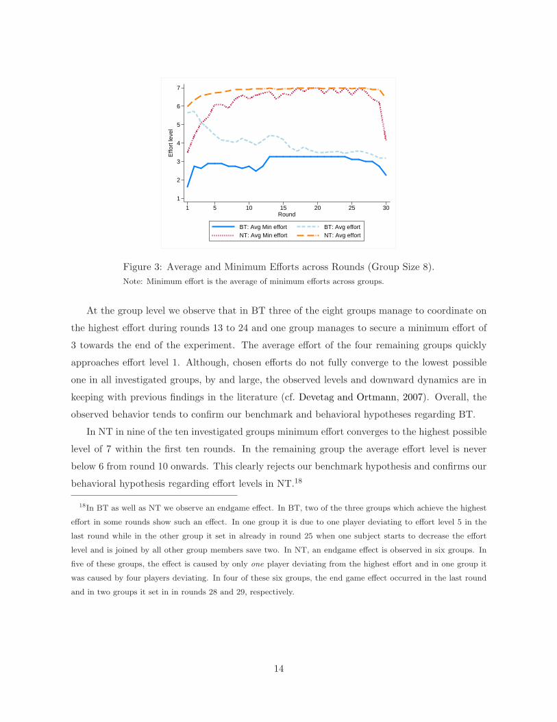
Figure 3: Average and Minimum Efforts across Rounds (Group Size 8).

Note: Minimum effort is the average of minimum efforts across groups.

At the group level we observe that in BT three of the eight groups manage to coordinate on

the highest effort during rounds 13 to 24 and one group manages to secure a minimum effort of

3 towards the end of the experiment. The average effort of the four remaining groups quickly

approaches effort level 1. Although, chosen efforts do not fully converge to the lowest possible

one in all investigated groups, by and large, the observed levels and downward dynamics are in

keeping with previous findings in the literature (cf. Devetag and Ortmann, 2007). Overall, the

observed behavior tends to confirm our benchmark and behavioral hypotheses regarding BT.

In NT in nine of the ten investigated groups minimum effort converges to the highest possible

level of 7 within the first ten rounds. In the remaining group the average effort level is never

below 6 from round 10 onwards. This clearly rejects our benchmark hypothesis and confirms our

behavioral hypothesis regarding effort levels in NT.18

18In BT as well as NT we observe an endgame effect. In BT, two of the three groups which achieve the highest

effort in some rounds show such an effect. In one group it is due to one player deviating to effort level 5 in the

last round while in the other group it set in already in round 25 when one subject starts to decrease the effort

level and is joined by all other group members save two. In NT, an endgame effect is observed in six groups. In

five of these groups, the effect is caused by only one player deviating from the highest effort and in one group it

was caused by four players deviating. In four of these six groups, the end game effect occurred in the last round

and in two groups it set in in rounds 28 and 29, respectively.

14

5.2 Size and Development of Interaction Neighborhoods

In NT, where interaction choices are endogenous, it is important to know whether interactions

actually take place, because only then high effort levels also have a high economic return. Recall

that, for any pair of subjects an interaction proposal results in actual interaction only if both

sides propose an interaction. If a pair of subjects does not interact this can be due to either

mutual or unilateral exclusion (i.e., either none or only one of both involved subjects proposes

to interact with each other).

0

.1

.2

.3

.4

.5

.6

.7

.8

.9

1

Fre

quen

cy

1 5 10 15 20 25 30Round

Mutual exclusionUnilateral exclusionInteraction

Figure 4: Frequency of Interactions and Exclusions across Rounds (Group Size 8).

Figure 4 depicts the frequencies of these three possible situations over time. In the first

round, on average, 99 percent of all possible interactions are proposed and 78 percent actually

take place. Thereafter, there is a slight decrease in the frequency of actual interactions which

reaches its minimum of 74 percent in round 3. From there onwards, this frequency is almost

monotonically and significantly increasing over rounds (p < 0.0001, JT test, n = 10) and as of

round 9 it never drops below 94 percent. This increase in actual interactions is accompanied by

a simultaneous decrease in the frequency of unilateral exclusions (p < 0.0001, JT test, n = 10),

which decreases to practically zero.19

19In fact, as of round 10, in all but one group all possible interactions take place in each round. The one group

where sometimes not all members interact with each other is the same group that do not fully settle on everybody

always choosing the highest effort of 7. Recall, however, that also in this group averaged effort never falls below 6.

15

5.3 Exclusion as Efficiency Enforcement

Here we examine if low effort providers are excluded by higher effort providers and, if yes, whether

being excluded makes the former to increase subsequently chosen effort levels. If that turns out

to be the case it would explain the observed parallel dynamics of effort levels and interaction

frequencies.

Specifically, we look at the changes in dyadic relationships for all pairs of group members, i

and j, and their effort choices in all three-rounds intervals from t− 1 to t and t+1. We do so in

three steps. First, we compare the effort levels of i and j in t− 1. Second, we analyze whether

j excludes i from her interaction neighborhood in t and how this depends on the chosen effort

levels in t− 1. Third, we check how the chosen effort level of i in t+ 1 compares with her effort

level in t − 1, and how a change in effort depends on having been a low effort provider in t − 1

and on being excluded in t.

For the first step we categorize all dyadic relations into three distinct classes in dependence

of the relative efforts of i and j in t − 1. The first class includes all cases where i provided at

least as high an effort as j (ei ≥ ej). The second class consists of the cases where i provided a

lower effort than j but a higher effort than the lowest effort in j’s neighborhood (ei < ej but

ei > mink∈Nj{ek}). The third class includes the cases where i’s effort was lower than j’s and

also the lowest effort in j’s neighborhood (ei < ej and ei = mink∈Nj{ek}). In the second step we

examine for each of these classes the frequency of exclusion of i by j in round t.

The upper panels, t−1 and t, of Table 2 report the results. Panel t−1 restates the introduced

classes of relative efforts between i and j. Panel t reports for each class the frequency (in percent)

of severed links, i.e., the exclusion rate, together with the number of cases in parentheses. From

the leftmost column it can be seen that, when i chooses an effort level that is not lower than the

effort level of j, the exclusion rate is negligible (0.6 percent). In stark contrast, when i chooses a

lower effort level than j, but is not the lowest effort provider in j’s interaction neighborhood, the

risk of being excluded from j’s neighborhood is quite high (23.6 percent) and further increases

to 38.5 percent when i is the lowest effort provider in j’s neighborhood (middle and rightmost

columns, respectively). To test whether these differences in exclusion rates across effort classes

are statistically significant, we calculate the exclusion rates for each class and each independent

matching group separately and apply aWilcoxon signed-rank test. All three pairwise comparisons

are significant (0.6 < 23.6, p = 0.039, n = 8; 23.6 < 38.5, p = 0.016, n = 8; 0.6 < 38.8, p = 0.002,

16

Table 2: Exclusion Rates and Responses to Exclusion.

t− 1 Effort of i relative to effort of jand efforts in j’s neighborhood

ei ≥ ej ei < ej ei < ejbut and

ei > mink∈Nj{ek} ei = mink∈Nj

{ek}

t exclusion rates (in percent)

0.6 23.6 38.5

(89/14738) (21/89) (105/273)

t+ 1 i’s response (in percent)

j ∈ Ii j 6∈ Ii j ∈ Ii j 6∈ Ii j ∈ Ii j 6∈ Ii

ei ↑ 11.8 2.6 71.4 9.5 61.6 10.1(9) (2) (15) (2) (61) (10)

ei = 68.4 14.4 4.8 4.8 18.2 0.0(52) (11) (1) (1) (18) (0)

ei ↓ 1.3 1.3 9.5 0.0 10.1 0.0(1) (1) (2) (0) (10) (0)

Note: In panel t, number of cases where exclusion takes places and totalnumber of cases in parentheses. In panel t + 1, j ∈ Ii (j /∈ Ii) indicates thecases where a subject i excluded in t by j proposes (does not propose) aninteraction link to its excluder j in t+ 1; number of cases in parentheses.

n = 10).20 Hence, higher effort providers indeed frequently exclude lower effort providers from

their interaction neighborhoods.

In the third step, we examine whether the observed exclusion actually affects subsequently

chosen effort levels of excluded subjects. To this end, we investigate the change in chosen effort

levels from period t − 1 to t + 1 for those cases where i was excluded in round t. An excluded

subject can react in two dimensions. First, it may keep the interaction proposal to j (j ∈ Ii)

or avoid interaction with j (j 6∈ Ii) in t + 1. Second, it may not change the effort level (ei=),

increase it (ei ↑) or decrease it (ei ↓).

Panel t+ 1 of Table 2 reports the results.21 Interestingly, excluded subjects overwhelmingly

keep their interaction proposal with those who excluded them. In between 81.5 percent (for

20The differences remain significant at the 5 percent level also after correcting for multiple comparisons using

the false discovery rate procedure (Benjamini and Hochberg, 1995).

21Note that the sum of cases in round t + 1 can be lower than in round t because for t = 30 no further round

exists.

17

ei ≥ ej) and 89.9 percent (for ei < ej and ei = mink∈Nj{ek}) of the cases excluded subjects keep

their interaction proposal with the excluding subject (see columns j ∈ Ii in Table 2, panel t+1).

Further, low effort providers (i,e., when ei < ej) strongly respond to exclusion with an increase

in effort levels. Specifically, in 80.9 and 71.7 percent of the cases an excluded low effort provider

increased her effort in response to being excluded (see, Table 2, row ei ↑ for the second and third

relative effort category, respectively). If a subject was excluded although it did not provide less

effort than the excluder then effort mostly stayed the same (82.8 percent, see row ei= for the

first relative effort category).22 Thus, exclusion indeed makes low effort providers subsequently

increase their effort levels and does not discourage high effort providers.

As discussed in Section 3.2, exclusion of low effort providers, while keeping own effort level

high, can have different short-term effects on the excluding subject’s earnings. First, it may

increase earnings because exclusion can increase the minimum effort in the remaining neighbor-

hood, which may overcompensate the loss from fewer interactions. Second, due to the negative

effect on earnings that comes with a reduction in the set of neighbors, an excluding subject

may incur losses in the short-term. In the first case exclusion is consistent with myopic earn-

ings maximization, whereas the second case is reminiscent of costly punishment in public goods

games (see, e.g., Fehr and Gachter, 2000). Overall, in a little less than half of all cases (48.2

percent) where a subject drops at least one interaction link to any of her neighbors this leads to

an increase in the excluding subject’s short-term earnings. In the remaining 51.8 percent of the

cases it actually lowers the short-term earnings of the excluding subjects. Note that, as argued

in Section 3.2, in both cases exclusion can be consistent with long-term earnings maximization

and efficiency considerations, when excluding subjects assume that those excluded will increase

their effort levels in response to exclusion.

In summary, high effort providers often exclude lower effort providers from their interaction

neighborhood, even though this sometimes comes at short-term costs. In response, lower effort

providers increase their effort levels and are eventually included again. This explains the strong

dynamics toward the highest possible effort level of 7 where everybody interacts with everybody

else (cf. Sections 5.1 and 5.2).

22Ideally we could provide a statistical test showing that in comparison to not excludes subjects, those who face

exclusion increase effort levels significantly more. However, there are too few cases where low effort providers are

not excluded by any neighbor. (Note, that the 23.6 and 38.5 percent refer to the excluding subject j and not to

the excluded subject i.)

18

5.4 Welfare

Failure of (efficient) coordination can be the source of large welfare losses. VHBB distinguish two

types of coordination failure. First, players may fail to predict the effort levels of other players

and, therefore, fail to coordinate on any equilibrium (individual coordination problem). Second,

players may coordinate, but do so on inefficient equilibria (collective coordination problem). In

the previous sections we have seen that in both treatments the individual coordination problem

is solved over time. However, the collective coordination problem is only solved in NT and, as

shown above, the mechanism behind this is exclusion. Yet, whenever a player excludes another

player the excluded player loses earnings for sure and the excluding player loses earnings in more

than 50 percent of the cases (see above). Therefore, at the outset it is not clear whether the

overall earnings in NT are higher than in BT.

In order to examine that, we calculate a group’s welfare as the sum of earnings of all group

members. In addition, we calculate the maximally possible welfare where every group member

chooses the highest effort level of 7 and interacts with all other group members (‘optimal bench-

mark’). Figure 5 shows the average welfare levels over time for both treatments as well as the

optimal benchmark.

0

200

400

600

800

1040

Ear

ning

s

1 5 10 15 20 25 30Round

Optimal benchmark BT NT

Figure 5: Welfare Levels across Rounds (Group Size 8).

In both treatments average welfare levels are significantly increasing over rounds (p < 0.0001,

n = 8 and n = 10, respectively, JT test for trend). In BT this is mainly due to a decrease in

the individual coordination problem. That is, subjects learn to coordinate on the same effort

level (cf. Section 5.1 and Figure 3). In NT, in contrast, the stark increase in welfare is induced

by overcoming both the individual and the collective coordination problem. As of round 10 up

19

to almost the last round welfare is basically identical to optimal welfare. Taken over all rounds,

average welfare in NT is economically and statistically significantly larger than in BT (BT: 629.5,

NT: 913.1, p = 0.0129, n = 18, Mann-Whitney test). Hence, endogenous neighborhood choice

not only increases effort levels but also welfare.

5.5 Large Groups

The experimental literature discussed in the Introduction unambiguously shows that for groups of

size larger than 12, eventual convergence of behavior towards inefficient equilibria is unavoidable.

The reason for this sober result is that strategic uncertainty is strongly increasing with group

size. Indeed, in fixed groups it usually suffices that one group member deviates to a lower effort

to initiate the unravelling of higher effort choices. With our XL treatments—with groups of size

24—we want to test whether neighborhood choice can also successfully ban strategic uncertainty

when groups become large.

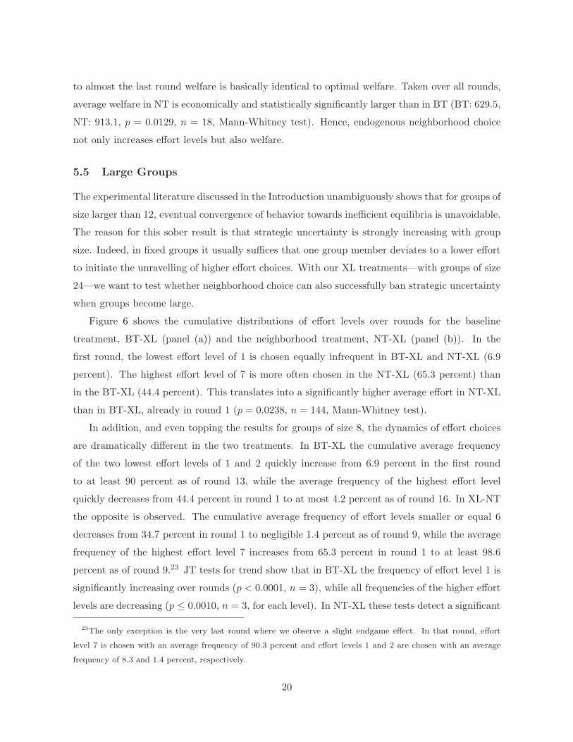
Figure 6 shows the cumulative distributions of effort levels over rounds for the baseline

treatment, BT-XL (panel (a)) and the neighborhood treatment, NT-XL (panel (b)). In the

first round, the lowest effort level of 1 is chosen equally infrequent in BT-XL and NT-XL (6.9

percent). The highest effort level of 7 is more often chosen in the NT-XL (65.3 percent) than

in the BT-XL (44.4 percent). This translates into a significantly higher average effort in NT-XL

than in BT-XL, already in round 1 (p = 0.0238, n = 144, Mann-Whitney test).

In addition, and even topping the results for groups of size 8, the dynamics of effort choices

are dramatically different in the two treatments. In BT-XL the cumulative average frequency

of the two lowest effort levels of 1 and 2 quickly increase from 6.9 percent in the first round

to at least 90 percent as of round 13, while the average frequency of the highest effort level

quickly decreases from 44.4 percent in round 1 to at most 4.2 percent as of round 16. In XL-NT

the opposite is observed. The cumulative average frequency of effort levels smaller or equal 6

decreases from 34.7 percent in round 1 to negligible 1.4 percent as of round 9, while the average

frequency of the highest effort level 7 increases from 65.3 percent in round 1 to at least 98.6

percent as of round 9.23 JT tests for trend show that in BT-XL the frequency of effort level 1 is

significantly increasing over rounds (p < 0.0001, n = 3), while all frequencies of the higher effort

levels are decreasing (p ≤ 0.0010, n = 3, for each level). In NT-XL these tests detect a significant

23The only exception is the very last round where we observe a slight endgame effect. In that round, effort

level 7 is chosen with an average frequency of 90.3 percent and effort levels 1 and 2 are chosen with an average

frequency of 8.3 and 1.4 percent, respectively.

20

downward trend for all effort levels strictly smaller than 7 (p ≤ 0.0225, n = 3, for all levels),

while the frequency of the highest effort level exhibits a significant trend upwards (p < 0.0001,

n = 3).

0

.1

.2

.3

.4

.5

.6

.7

.8

.9

1

Ave

rage

freq

uenc

y of

effo

rt le

vels

1 5 10 15 20 25 30Round

Effort 7 Effort 6 Effort 5 Effort 4Effort 3 Effort 2 Effort 1

(a) Baseline Treatment

0

.1

.2

.3

.4

.5

.6

.7

.8

.9

1

Ave

rage

freq

uenc

y of

effo

rt le

vels

1 5 10 15 20 25 30Round

Effort 7 Effort 6 Effort 5 Effort 4Effort 3 Effort 2 Effort 1

(b) Neighborhood Treatment

Figure 6: Cumulative Distribution of Efforts across Rounds (Group Size 24).

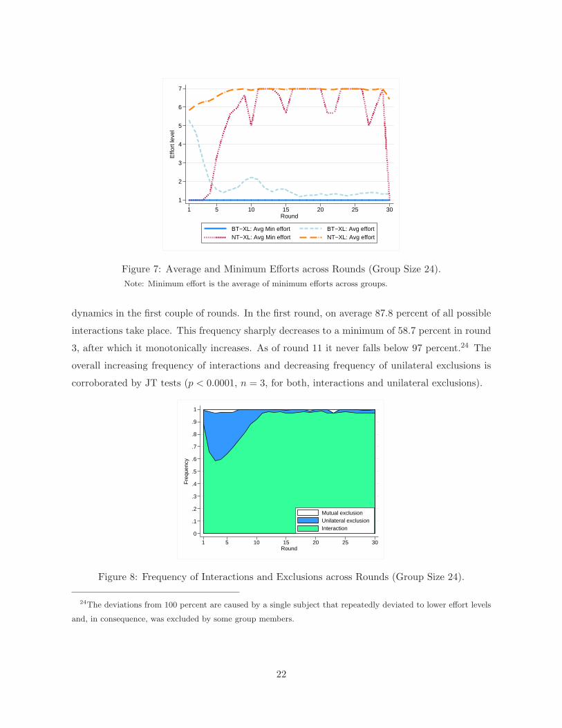
Figure 7 shows the average effort levels and the average minimum effort levels for both

treatments. Over rounds the average effort is significantly decreasing in BT-XL (p < 0.0001,

n = 3, JT test) but significantly increasing in NT-XL (p < 0.0001, n = 3, JT test). The

average minimum effort in BT-XL does not exhibit any trend because it is at the lowest level of

1 throughout all rounds. In NT-XL this effort statistics shows a significant increase over time

(p < 0.0001, n = 3, JT test). Furthermore, when averaging across rounds, each investigated

NT-XL group achieves average and average minimum effort levels that exceed the levels of their

counterparts in BT-XL by far (average effort: 1.78 in BT-XL, 6.83 in NT-XL; average minimum

effort: 1 in BT-XL, 5.41 in NT-XL). These differences are statistically significant at p = 0.10

(MW tests), which is the lowest achievable p-value for the two-sided test, given that the number

of our independent matching groups is 2× 3.

Figure 7 indicates an endgame effect which is due to only a few subjects. In the different

NT-XL groups 1, 2, and 4, respectively, of the 24 group members deviated from the highest effort

level in the last round. The occasional downward movements of the average minimum effort are

caused by a single individual in a single group. In the other two groups all members choose the

highest effort as of round 10.

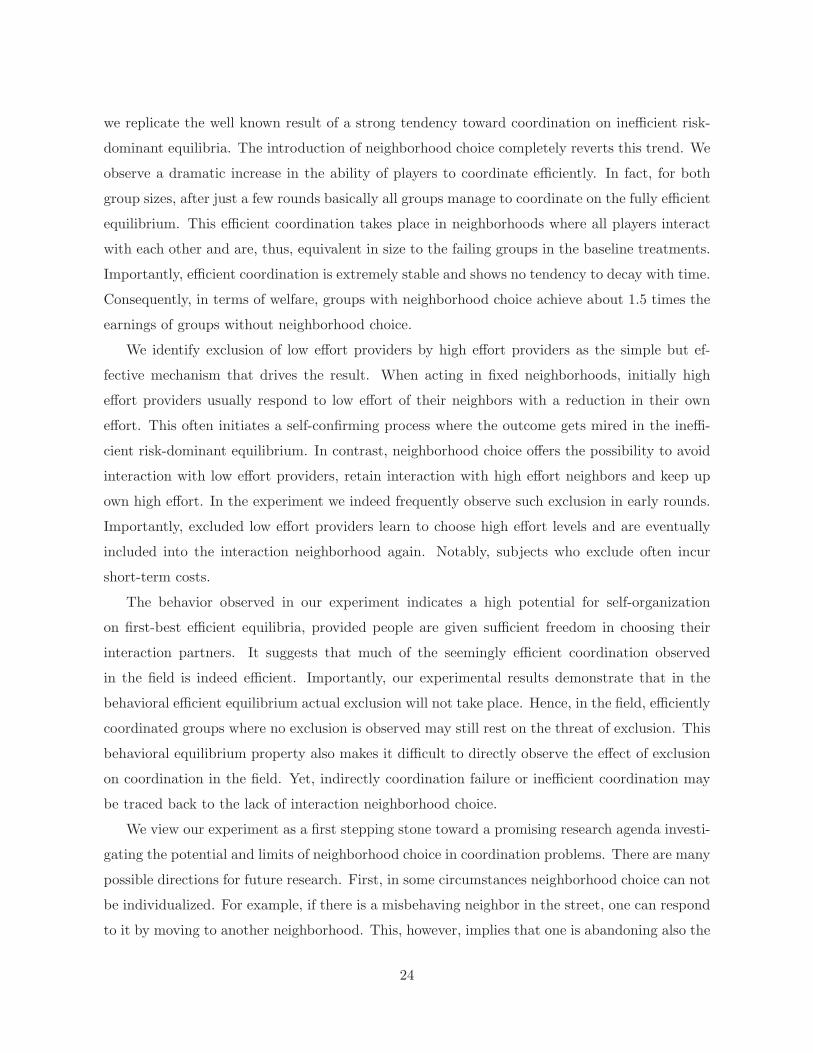
The development of actual interactions and unilateral and mutual exclusions is depicted in

Figure 8. The picture is qualitatively the same as for groups of size 8 but with a more pronounced

21

1

2

3

4

5

6

7

Effo

rt le

vel

1 5 10 15 20 25 30Round

BT−XL: Avg Min effort BT−XL: Avg effort NT−XL: Avg Min effort NT−XL: Avg effort

Figure 7: Average and Minimum Efforts across Rounds (Group Size 24).

Note: Minimum effort is the average of minimum efforts across groups.

dynamics in the first couple of rounds. In the first round, on average 87.8 percent of all possible

interactions take place. This frequency sharply decreases to a minimum of 58.7 percent in round

3, after which it monotonically increases. As of round 11 it never falls below 97 percent.24 The

overall increasing frequency of interactions and decreasing frequency of unilateral exclusions is

corroborated by JT tests (p < 0.0001, n = 3, for both, interactions and unilateral exclusions).

0

.1

.2

.3

.4

.5

.6

.7

.8

.9

1

Fre

quen

cy

1 5 10 15 20 25 30Round

Mutual exclusionUnilateral exclusionInteraction

Figure 8: Frequency of Interactions and Exclusions across Rounds (Group Size 24).

24The deviations from 100 percent are caused by a single subject that repeatedly deviated to lower effort levels

and, in consequence, was excluded by some group members.

22

Exclusion behavior is also very similar to that observed for groups of size 8. Subjects providing

a lower effort are excluded by subjects choosing a higher effort. Specifically, in each case where

a subject chooses an effort below the highest possible effort level it is excluded by at least one

group member. In response to being excluded subjects increase their effort level to the highest

level, after which they receive interaction proposals from all group members again.25

In both treatments welfare increases over rounds (p < 0.0001, n = 3, JT tests). Yet, the

opposing dynamics in effort choices between BT-XL and NT-XL together with the convergence

toward full interaction in NT-XL implies welfare effects that are strongly in favor of the neigh-

borhood treatment. As of round 6, total welfare achieved in NT-XL is above the one achieved

in BT-XL. Furthermore, in BT-XL actual welfare never exceeds 52.5 percent (round 17) of the

optimally achievable welfare level, while in NT-XL it almost never falls below 94.7 percent of the

optimal level as of round 11. Across all rounds, the achieved average welfare in BT-XL (1492.6)

is only 61 percent of the welfare achieved in NT-XL (2443.6). The difference is statistically sig-

nificant at p = 0.10 (MW test). As for effort levels this is the lowest p-value that can be achieved

for the two-sided test, given that the number of our independent matching groups is 2× 3.

6 Conclusion

In this paper we study the effect of neighborhood choice on behavior in weakest-link (aka mini-

mum effort) coordination games. Theoretically, the introduction of neighborhood choice, which

expands the strategy space, worsens the coordination problem as it hugely increases the number

of pure strategy Nash equilibria. Moreover, from an equilibrium selection perspective, neighbor-

hood choice seems irrelevant for the investigated games because the unique stochastically stable

equilibrium prescribes that everybody plays the inefficient risk-dominant equilibrium. However,

these theoretical considerations neglect that neighborhood choice may provide room for psycho-

logical motivations like a desire for efficiency to affect behavior differently than in games played

in fixed interaction neighborhoods.

To test the behavioral effect of neighborhood choice we conduct experiments with groups

of size 8 and 24. In the baseline treatments with exogenously fixed interaction neighborhoods,

25The only exception is the one subject mentioned in footnote 24. After repeated deviations from the highest

effort level some group members became ever more reluctant to interact with this subject and at some point

excluded it for good. On average this subject only received 5 (out of 23) interaction proposals per round, whereas

the remaining subjects received 21 proposals per round, on average.

23

we replicate the well known result of a strong tendency toward coordination on inefficient risk-

dominant equilibria. The introduction of neighborhood choice completely reverts this trend. We

observe a dramatic increase in the ability of players to coordinate efficiently. In fact, for both

group sizes, after just a few rounds basically all groups manage to coordinate on the fully efficient

equilibrium. This efficient coordination takes place in neighborhoods where all players interact

with each other and are, thus, equivalent in size to the failing groups in the baseline treatments.

Importantly, efficient coordination is extremely stable and shows no tendency to decay with time.

Consequently, in terms of welfare, groups with neighborhood choice achieve about 1.5 times the

earnings of groups without neighborhood choice.

We identify exclusion of low effort providers by high effort providers as the simple but ef-

fective mechanism that drives the result. When acting in fixed neighborhoods, initially high

effort providers usually respond to low effort of their neighbors with a reduction in their own

effort. This often initiates a self-confirming process where the outcome gets mired in the ineffi-

cient risk-dominant equilibrium. In contrast, neighborhood choice offers the possibility to avoid

interaction with low effort providers, retain interaction with high effort neighbors and keep up

own high effort. In the experiment we indeed frequently observe such exclusion in early rounds.

Importantly, excluded low effort providers learn to choose high effort levels and are eventually

included into the interaction neighborhood again. Notably, subjects who exclude often incur

short-term costs.

The behavior observed in our experiment indicates a high potential for self-organization

on first-best efficient equilibria, provided people are given sufficient freedom in choosing their

interaction partners. It suggests that much of the seemingly efficient coordination observed

in the field is indeed efficient. Importantly, our experimental results demonstrate that in the

behavioral efficient equilibrium actual exclusion will not take place. Hence, in the field, efficiently

coordinated groups where no exclusion is observed may still rest on the threat of exclusion. This

behavioral equilibrium property also makes it difficult to directly observe the effect of exclusion

on coordination in the field. Yet, indirectly coordination failure or inefficient coordination may

be traced back to the lack of interaction neighborhood choice.

We view our experiment as a first stepping stone toward a promising research agenda investi-

gating the potential and limits of neighborhood choice in coordination problems. There are many

possible directions for future research. First, in some circumstances neighborhood choice can not

be individualized. For example, if there is a misbehaving neighbor in the street, one can respond

to it by moving to another neighborhood. This, however, implies that one is abandoning also the

24

nice neighbors who do behave. Another example are work teams where one can choose the team

one would like to be a member of but not the team composition itself. Second, physically moving

often comes with transactions costs. In our experiment this is reflected by the opportunity costs

of not interacting. Yet, the introduction of nominal costs when abandoning an interaction may

have other behavioral effects than mere opportunity costs. Third, an obvious candidate for fu-

ture research is the exploration of information effects. In our experiment subjects possess global

information and have perfect recall in the sense that they can access all decisions in all past

periods for all members in their group, even if they did not interact with them. An interesting

variation would be to give only local information where only effort choices of interaction partners

can be observed. Further, there are many more possible directions of research like the evaluation

of the effect of other than a proportional increase of the payoff with the neighborhood size or

the effect of limits on the number of neighbors one can interact with, to mention just a few.

Last but not least, our results suggest an important implication for the design of organizations

and institutions. In particular, it provides a policy dimension that is probably cheaper than

increasing the payoff for coordination on the efficient equilibrium (Brandts and Cooper, 2006)

and more effective than exogenously growing groups (Weber, 2006).

25

References

Battalio, R., Samuelson, L., and Van Huyck, J. (2001). Optimization incentives and coordination

failure in laboratory stag hunt games. Econometrica, 69(3):749–764.

Benjamini, Y. and Hochberg, Y. (1995). Controlling the false discovery rate: A practical and

powerful approach to multiple testing. Journal of the Royal Statistical Society, 57(1):289–300.

Berninghaus, S. K. and Ehrhart, K.-M. (1981). Time horizon and equilibrium selection in tacit

coordination games: Experimental results. Journal of Economic Behavior and Organization,

37(2):231–248.

Berninghaus, S. K. and Ehrhart, K.-M. (2001). Coordination and information: Recent experi-

mental evidence. Economics Letters, 73(3):345–351.

Blume, A. and Ortmann, A. (2007). The effects of costless pre-play communication: Exper-

imental evidence from games with Pareto-ranked equilibria. Journal of Economic Theory,

132:274–290.

Bolton, G. and Ockenfels, A. (2000). ERC: A theory of equity, reciprocity, and competition.

American Economic Review, pages 166–193.

Bornstein, G., Gneezy, U., and Nagel, R. (2002). The effect of intergroup competition on group

coordination: An experimental study. Games and Economic Behavior, 41(1):1–25.

Brandts, J. and Cooper, D. J. (2006). A change would do you good .... An experimental study

on how to overcome coordination failure in organizations. The American Economic Review,

96(3):669–693.

Brandts, J. and Cooper, D. J. (2007). Its what you say, not what you pay: An experimental

study of manageremployee relationships in overcoming coordiantion failure. Journal of the

European Economic Association, 5(6):1223–1268.

Brandts, J., Cooper, D. J., and Fatas, E. (2007). Leadership and overcoming coordination failure

with asymmetric costs. Experimental Economics, 10(3):269–284.

Cachon, G. P. and Camerer, C. F. (1996). Loss-avoidance and forward induction in experimental

coordination games. The Quarterly Journal of Economics, pages 165–194.

Camerer, C. (2003). Behavioral game theory: Experiments in strategic interaction. Princeton

University Press, New York and Princeton.

Charness, G. (2000). Self-serving cheap talk: A test of Aumann’s conjecture. Games and

Economic Beahvior, 33(2):177–194.

Charness, G. and Rabin, M. (2002). Understanding social preferences with simple tests. Quarterly

26

Journal of Economics, 117:817–869.

Chaudhuri, A., Schotter, A., and Sopher, B. (2009). Talking ourselves to efficiency: Coordina-

tion in inter-generational minimum effort games with private, almost commen and common

knowledge of advice. The Economic Journal, 119(1):91–122.

Chen, R. and Chen, Y. (2011). The potential of social identity for equilibrium selection. American

Economic Review, 101(6):2562–2589.

Cooper, R. (1999). Coordination Games: Complementarities and Macroeconomics. Cambridge

University Press, Cambridge, UK.

Cooper, R., DeJong, D. V., Forsythe, R., and Ross, T. W. (1992). Communication in coordination

games. The Quarterly Journal of Economics, 107(2):739–771.

Corbae, D. and Duffy, J. (2008). Experiments with network formation. Games and Economic

Behavior, 64(1):81 – 120.

Corten, R. and Buskens, V. (2010). Co-evolution of conventions and networks: An experimental

study. Social Networks, 32(1):4–15.

Crawford, V. P. (1995). Adaptive dynamics in coordination games. Econometrica, 63(1):103–143.

Cuzick, J. (1985). A Wilcoxon-type test for trend. Statistics in Medicine, 4:87–90.

Devetag, G. and Ortmann, A. (2007). When and why? A critical survey on coordination failure

in the laboratory. Experimental Economics, 10(2):171–178.

Engelmann, D. and Normann, H.-T. (2010). Maximum effort in the minimum-effort game.

Experimental Economics, 13(3):249–259.

Engelmann, D. and Strobel, M. (2004). Inequality aversion, efficiency, and maximin preferences

in simple distribution experiments. The American Economic Review, 94(4):857–869.

Fehr, E. and Gachter, S. (2000). Cooperation and punishment in public goods experiments.

American Economic Review, 90:980–994.

Fehr, E. and Schmidt, K. (1999). A theory of fairness, competition, and cooperation. Quarterly

Journal of Economics, 114:817–868.

Feri, F., Irlenbusch, B., and Sutter, M. (2010). Efficiency gains from team-based coordination—

Large-scale experimental evidence. American Economic Review, 100(4):1892–1912.

Fischbacher, U. (2007). z-tree: Zurich toolbox for ready-made economic experiments. Experi-

mental Economics, 10(2):171–178.

Goeree, J. K. and Holt, C. A. (2001). Ten little treasures of game theory and ten intuitive

contradictions. The American Economic Review, 91(5):1402–1422.

Hamman, J., Rick, S., and Weber, R. A. (2007). Solving coordination failure with “all-or-none”

27

group-level incentives. Experimental Economics, 10(3):285–303.

Harrison, G. W. and Hirshleifer, J. (1989). An experimental evaluation of weakest link/best shot

models of public goods. Journal of Political Economy, 97(1):201–225.

Harsanyi, J. C. and Selten, R. (1988). Ageneral theory of equilibrium selection in games. MIT

Press, Cambridge, Mass.

Hirshleifer, J. (1983). From weakest-link to best-shot: The voluntary provision of public goods.

Public Choice, 41(3):371–386.

Jackson, M. andWatts, A. (2002). On the formation of interaction networks in social coordination

games. Games and Economic Behavior, 41(2):265–291.

Knez, M. and Camerer, C. (1994). Creating expectational assets in the laboratory: Coordination

in ‘weakest-link’ games. Strategic Management Journal, 15:101–119.

Kogan, S., Kwasnica, A. M., and Weber, R. A. (2011). Coordination in the presence of asset

markets. The American Economic Review, 101(2):927–947.

McKelvey, R. D. and Palfrey, T. R. (1995). Quantal response equilibria for normal form games.

Games and Economic Behavior, 10:6–38.

Nordhaus, W. D. (2006). Paul Samuelson and global public goods. In Szenberg, M., Ramrattan,

L., and Gottesman, A., editors, Samuelsonian Economics, pages 88–98. Oxford University

Press, Oxford:UK.

Oechssler, J. (2011). Finitely repeated games with social preferences. Discussion Paper Series

No. 512, Department of Economics, University of Heidelberg.

Pirie, W. (1983). Jonckheere tests for ordered alternatives. In Samuel, K., Lloyd, J. N., and B.,

R. C., editors, Encyclopedia of statistical sciences, volume 4. John Wiley, New York.

Sandler, T. (1998). Global and regional public goods: A prognosis for collective action. Fiscal

Studies, 19(3):221–247.

Schelling, T. C. (1980). The Strategy of Conflict. Harvard University Press.

Van Huyck, J. B., Battalio, R. C., and Beil, R. O. (1990). Tacit coordination games, strategic

uncertainty, and coordination failure. The American Economic Review, 80(1):234–248.

Weber, R., Camerer, C., Rottenstreich, Y., and Knez, M. (2001). The illusion of leadership:

Misattribution of cause in coordination games. Organizational Science, 12(5):582–598.

Weber, R. A. (2006). Managing growth to achieve efficient coordination in large groups. The

American Economic Review, 96(1):114–126.

Young, H. P. (1993). The evolution of conventions. Econometrica, 61:57–84.

Young, H. P. (1998). Individual Strategy and Social Structure. Princeton University Press.

28

Appendix

A Theoretical Benchmarks

We show that for our parameter setting the fully interlinked network with every player playing the lowest

effort is the unique stochastically stable equilibrium for the minimum effort game with neighborhood

choice (NG). Thereafter we show that this also holds for the restricted case of the minimum effort game

without neighborhood choice.

A.1 The Game

The analysis rests on a one-shot game where each player simultaneously chooses an effort level and the

set of other players whom he or she wants to interact with. The basic elements of the game are:

• N = {1, 2, 3, ..., n} is a finite set of players.

• E = {1, 2, ...,m} is a finite set of effort levels.

• si = (ei, Ii) is the strategy of player i with ei ∈ E is the player’s chosen effort level and Ii ⊆ N \{i}

is the set of players with whom i wants to interact with.

• s = (s1, ..., sn) = ((ej , Ij))j∈Nis a strategy profile. Later we will interpret it as a state in a

Markovian chain. With se we denote the strategy profile where every player wants to interact with

every other player and all play the same effort e, i.e. se = ((e, N \ {j}))j∈N .

• s−i = (s1, . . . , si−1, si+1, . . . , sn) = ((ej , Ij))j∈N\{i} is the vector of strategies of all players except

i.

• Given a strategy profile s, players i and j are linked if both want to interact with each other, i.e.

j ∈ Ii and i ∈ Ij . If an interaction proposal of i with j is not reciprocated, i.e. j ∈ Ii but i 6∈ Ij

then j is called a dangling link of i.

• Given a strategy profile s, the neighborhood of a player i is the set of all players to whom i is linked

to, i.e. Ni(s) = {j|j ∈ Ii ∧ i ∈ Ij}. With |Ni(s)| we denote the cardinality of Ni(s), in other words

the size of the neighborhood.

• For a given s player i’s payoff is

πi(s) =|Ni(s)|

n− 1

[

a

(

minj∈Ni(s)∪{i}

{ej}

)

− bei + c

]

with a > b > 0 and c > 0.

• Our specific experimental settings are m = 7, a = 20, b = 10 and c = 60 for n = 8 and n = 24,

respectively.

29

A.2 The Process

We follow a variant of the approach of Young (1993,1998). Assume discrete and successive time rounds

(t = 1, 2, ..). In each round t every player may play a myopic best response to the other players’ strategies

of round t − 1 with some positive probability σ. This construction constitutes a Markov chain with the

state space being the set of all strategy profiles and the transition probabilities depending on σ and the

payoffs π. We will show that only states with the complete network and everybody playing the same

effort are absorbing states and that no other recurrent class of states exist. Thereafter we take the

parametrization of our experimental design and calculate the number of errors which are necessary to get

from one absorbing state to the other. We use the method introduced by Young (1993,1998) to show that

the state with the complete network and the minimum effort played by all players is the only stochastically

stable one.

A.3 Some Useful Observations

To start, we state some almost trivial propositions. We will use them later. The corresponding proofs are

straightforward.

Proposition A.1 Given an outcome s = ((ei, Ii), s−i). Then player i’s payoff is independent of dangling

links, i.e. πi((ei, Ii), s−i) = πi((ei, I′i), s−i) with I ′i = {j|j ∈ Ii ∧ i ∈ Ij}.

Proof: Dangling links are not decisive for the neighborhood of a player, i.e.Ni((ei, Ii), s−i) = Ni((ei, I′i), s−i).

Hence neither the removal nor the addition of dangling links change payoffs. As a corollary we get that

any best response remains a best response if dangling links are removed or added. �

Proposition A.2 For Ni(s) 6= ∅ the condition ei = minj∈Ni(s){ej} is necessary for si = (ei, Ii) being a

best response to s−i = ((ej , Ij))j∈N\{i}.

Proof: Assume Ni(s) 6= ∅ and that the condition does not hold, then i can improve his payoff by

adjusting ei to minj∈Ni(s){ej} while holding Ii constant. �

A.4 Absorbing States and Recurrent Classes

Proposition A.3 A state se with sei = (e, N \{i}) for each player i ∈ N and some e ∈ E is an absorbing

state.

Proof: We have to show that si = (e, N \ {i}) is the only best response to s−i = (sj)j∈N\{i} with

sj = (e, N \ {j}).

Removing players from Ii strictly decreases |Ni(s)| and therefore strictly decreases πi. The marginal

payoff change with respect to ei is −a + b (< 0) if i decreases ei and −b (< 0) if i increases ei. Any

30

combination of changes in effort and interaction also leads to negative payoff consequences. It follows that

si is the only best response to s−i. This holds for each player. �

Each of the absorbing states forms a recurrent class. In the following we will show that no other

recurrent class exists.

Proposition A.4 No other recurrent class than those defined by the absorbing states in Proposition A.3

exists.

Proof: We introduce a hierarchy of sets of states into the state space. Let

S be the set of all possible states.

S′ be the subset of S for which in any state s′ players who are linked play the same effort level and no

dangling link exists. This means that the network induced by s′ consists of one or more components

with all players within a component are playing the same effort level.

S′′ be the subset of S′ where in any state s′′ the link relation is transitive, i.e. if i is linked to j and j

to k then also i is linked to k. This means that the network induced by s′′ consists of one or more

fully interlinked components without dangling links and with all players within a component are

playing the same effort level.

Sa be the set of absorbing states as defined in Proposition A.3.

It is obvious that S ⊃ S′ ⊃ S′′ ⊃ Sa. The last inclusion follows from Proposition A.3, an absorbing

state is characterized by the complete network with every player playing the same effort.

The proof comprises three steps. We will show that for each state in the supersets S, S′, and S′′ a

finite path of best responses into the subsets S′, S′′, and Sa exists which the players follow with positive

probability.

Step s ∈ S → s′ ∈ S′

Assume state s ∈ S. The following algorithm generates a finite sequence of best responses that occurs

with positive probability and leads to a state s′ ∈ S′. Assume that players update their strategies one by

one.

1. Sort the players into a two lists A and B.26

List A contains players that do not have any dangling link in their strategy and whose effort level

is at most the minimum effort level of their neighborhood.

26We chose to have lists rather than sets because list B must enable an order for processing the elements (first

in first out principle).

31

List B contains the other players.

2. Take the first player i from list B and calculate all best responses to s−i. There exists a best

response si without dangling links and ei = minj∈Ni(s){ej} (see propositions A.1 and A.2). Update

player i’s strategy to such a best response and put him at the end of list A. The update of si may

cause some players in A to violate the A-conditions. Put them at the end of list B.

3. If there are players left in B then continue with step 2.

The generated sequence is finite because for each application of step 2 there is exactly one player moving

from B to A. A move of a player i from A to B can only happen if a neighbor j moves from B to A and

breaks up a link or decreases his effort level such that ej < ei. In the first case the link between i and

j will be irreversibly deleted.27 In the second case i updates by keeping the link and lowering ei or by

breaking the link. Since E is finite, lowering ei can only happen a finite number of times before the link

has to be broken. Because the breaking of a link is irreversible and there is only a finite number of links

to be broken, there can only be a finite number of moves from A to B.

Step s′ ∈ S′ → s′′ ∈ S′′

Assume state s′ ∈ S′, i.e. N is subdivided into several disjoint components C1, C2, . . . , Ck. Each com-

ponent is (not necessarily fully) linked and is free of dangling links. Each player within a component is

playing the same effort level. Consider a component Cl in which effort level e is played. Consider further a

player i ∈ Cl who plays strategy si = (e, Ii) with Ii ⊆ Cl. Then strategy si = (e, Cl\{i}) is a best response

to s−i because adding dangling links do not change payoffs (see Proposition A.1). There is a positive

probability that each player is playing this best response and that this happens in each component. This

means that we reach a state s′′ ∈ S′′ where components are fully connected.

Step s′′ ∈ S′′ → sa ∈ Sa

Assume state s′′ ∈ S′′. Assume two disjoint components C,C ⊂ N and that each component is fully

connected. Each player in C and C plays effort e and e, respectively. Without loss of generality assume

that e ≥ e.

By the condition|C|+

∣

∣C∣

∣− 1

n− 1(ae− be+ c) >

∣

∣C∣

∣− 1

n− 1(ae− be+ c) (3)

we distinguish two cases:

27Note that only players moving from B to A may change their strategy. Player j who is now in A can only

reestablish the link to i, after he has been moved back to B. Since he will be put at the end of the list, i will have

deleted the dangling link before j’s next turn.

32

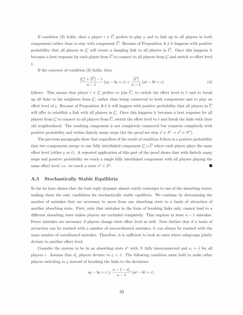
If condition (3) holds, then a player i ∈ C prefers to play e and to link up to all players in both

components rather than to stay with component C. Because of Proposition A.1 it happens with positive

probability that all players in C will create a dangling link to all players in C. Once this happens it

becomes a best response for each player from C to connect to all players from C and switch to effort level

e.

If the converse of condition (3) holds, then

|C|+∣

∣C∣

∣− 1

n− 1(ae− be+ c) <

∣

∣C∣

∣

n− 1(ae− be+ c) (4)

follows. This means that player i ∈ C prefers to join C, to switch the effort level to e and to break

up all links to his neighbors from C, rather than being connected to both components and to play an

effort level of e. Because of Proposition A.1 it will happen with positive probability that all players in C

will offer to establish a link with all players in C. Once this happens it becomes a best response for all

players from C to connect to all players from C, switch the effort level to e and break the links with their

old neighborhood. The resulting component is not completely connected but connects completely with

positive probability and within finitely many steps (for the proof see step s′ ∈ S′ → s′′ ∈ S′′).

The previous paragraphs show that regardless of the result of condition 3 there is a positive probability

that two components merge to one fully interlinked component C ∪ C where each player plays the same

effort level (either e or e). A repeated application of this part of the proof shows that with finitely many

steps and positive probability we reach a single fully interlinked component with all players playing the

same effort level; i.e. we reach a state sa ∈ Sa. �

A.5 Stochastically Stable Equilibria

So far we have shown that the best reply dynamic almost surely converges to one of the absorbing states,

making them the only candidates for stochastically stable equilibria. We continue by determining the

number of mistakes that are necessary to move from one absorbing state to a basin of attraction of

another absorbing state. First, note that mistakes in the form of breaking links only, cannot lead to a

different absorbing state unless players are excluded completely. This requires at least n − 1 mistakes.

Fewer mistakes are necessary if players change their effort level as well. Note further that if a basin of

attraction can be reached with a number of uncoordinated mistakes, it can always be reached with the

same number of coordinated mistakes. Therefore, it is sufficient to look at cases where subgroups jointly

deviate to another effort level.

Consider the system to be in an absorbing state sa with N fully interconnected and ei = e for all

players i. Assume that d↓ players deviate to e < e. The following condition must hold to make other

players switching to e instead of breaking the links to the deviators:

ae− be+ c ≥n− 1− d↓

n− 1(ae− be+ c) .

33

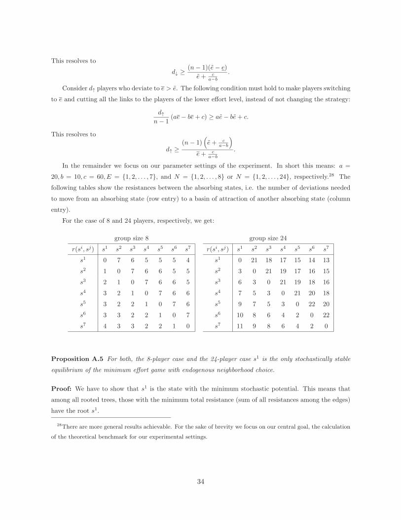
This resolves to

d↓ ≥(n− 1)(e− e)

e+ ca−b

.

Consider d↑ players who deviate to e > e. The following condition must hold to make players switching

to e and cutting all the links to the players of the lower effort level, instead of not changing the strategy:

d↑

n− 1(ae− be+ c) ≥ ae− be+ c.

This resolves to

d↑ ≥(n− 1)

(

e+ ca−b

)

e+ ca−b

.

In the remainder we focus on our parameter settings of the experiment. In short this means: a =

20, b = 10, c = 60, E = {1, 2, . . . , 7}, and N = {1, 2, . . . , 8} or N = {1, 2, . . . , 24}, respectively.28 The

following tables show the resistances between the absorbing states, i.e. the number of deviations needed

to move from an absorbing state (row entry) to a basin of attraction of another absorbing state (column

entry).

For the case of 8 and 24 players, respectively, we get:

group size 8 group size 24

r(si, sj) s1 s2 s3 s4 s5 s6 s7 r(si, sj) s1 s2 s3 s4 s5 s6 s7

s1 0 7 6 5 5 5 4 s1 0 21 18 17 15 14 13

s2 1 0 7 6 6 5 5 s2 3 0 21 19 17 16 15

s3 2 1 0 7 6 6 5 s3 6 3 0 21 19 18 16

s4 3 2 1 0 7 6 6 s4 7 5 3 0 21 20 18

s5 3 2 2 1 0 7 6 s5 9 7 5 3 0 22 20

s6 3 3 2 2 1 0 7 s6 10 8 6 4 2 0 22

s7 4 3 3 2 2 1 0 s7 11 9 8 6 4 2 0

Proposition A.5 For both, the 8-player case and the 24-player case s1 is the only stochastically stable

equilibrium of the minimum effort game with endogenous neighborhood choice.

Proof: We have to show that s1 is the state with the minimum stochastic potential. This means that

among all rooted trees, those with the minimum total resistance (sum of all resistances among the edges)

have the root s1.

28There are more general results achievable. For the sake of brevity we focus on our central goal, the calculation

of the theoretical benchmark for our experimental settings.

34

Consider a rooted tree Tm with root sm 6= s1 and total resistance r(Tm). Then we can construct a

new rooted tree Tm−1 with root sm−1 by connecting sm to sm−1 and removing the edge from sm−1 to

state sk on the path to sm. The new tree has total resistance

r(Tm−1) = r(Tm) + r(sm, sm−1)− r(sm−1, sk) ≤ r(Tm).

The last inequality holds because r(sm, sm−1) ≤ r(sm−1, sk) as can be verified from the tables.

We can iterate this process till we construct T 1 with root s1 and total resistance

r(T 1) = r(T 2) + r(s2, s1)− r(s1, sk) < r(T 2).

The last inequality holds because r(s2, s1) < r(s1, sk) as can be verified from the tables.

Hence, for any rooted tree Tm we find a chain of rooted trees such that r(T 1) < r(T 2) ≤ · · · ≤ r(Tm).

Therefore the root of the tree with the minimum total resistance must be s1. �

A.6 The Case without Neighborhood Choice

For the case without neighborhood choice Ii is restricted to Ii = N \ {i}. A strategy is therefore si = ei.

Furthermore Ni(s) = N \ {i} and hence |Ni(s)| = n− 1. This reduces the payoff function to

πi(s) = aminj∈N

{ej} − bei + c

Proposition A.6 A state s with si = e for each player i ∈ N and some e ∈ E is an absorbing state in

the minimum effort game without neighborhood choice and no other recurrent class exists.

Proof: This follows immediately from the restriction Ii = N \ {i} and Proposition A.2. �

The resistance tables for the case of 8 and 24 players, respectively, are:

group size 8 group size 24

r(si, sj) s1 s2 s3 s4 s5 s6 s7 r(si, sj) s1 s2 s3 s4 s5 s6 s7

s1 0 7 7 7 7 7 7 s1 0 23 23 23 23 23 23

s2 1 0 7 7 7 7 7 s2 1 0 23 23 23 23 23

s3 1 1 0 7 7 7 7 s3 1 1 0 23 23 23 23

s4 1 1 1 0 7 7 7 s4 1 1 1 0 23 23 23

s5 1 1 1 1 0 7 7 s5 1 1 1 1 0 23 23

s6 1 1 1 1 1 0 7 s6 1 1 1 1 1 0 23

s7 1 1 1 1 1 1 0 s7 1 1 1 1 1 1 0

Proposition A.7 For both, the 8-player case and the 24-player case s1 is the only stochastically stable

equilibrium of the minimum effort game without endogenous neighborhood choice.

The proof is identical to the proof of Proposition A.5.

35

B Instructions and Control Questions

[Remark: In the following we present the instructions and control questions for the neighborhood treat-

ment. The instructions for the baseline treatment were identical except the paragraphs marked with [NT]

and [*]. Paragraphs with [NT] were only given in the neighborhood treatment. Paragraphs with [*] were

given in both treatments but appropriately reformulated for the baseline treatment. A complete set of

instructions is available from the authors.]

B.1 Instructions for Groups of Size 8

Introduction

Welcome to this decision-making experiment. In this experiment you can earn money. How much you earn

depends on your decisions and the decisions of other participants. During the experiment your earnings

will be counted in points. At the end of the experiment you get your earned points paid out privately and

confidentially in cash, according to the exchange rate:

2 points = 1 eurocent.

It is important that you have a good understanding of the rules in the experiment. Therefore, please read

these instructions carefully. In order to check that the instructions are clear to you, you will be asked a

few questions at the end of the instructions. The experiment will start only after everybody has correctly

answered the questions. At the end of the experiment you will be asked to fill in a short questionnaire.

Thereafter you will receive your earnings.

During the whole experiment, you are not allowed to communicate with other participants

in any other way than specified in the instructions.

If you have a question, please raise your hand. We will then come to you and answer your question in

private.

Explanation Experiment

During the experiment every participant is in a group of eight, that is in a group with seven other

participants. The group you are in will not change during the experiment. You will not receive any

information about the identity of the persons in your group, neither during the experiment, nor after the

experiment. Other participants will also not receive any information about your identity.

36

Each person in your group is indicated by a letter. You will receive the name “me”. The other seven

persons in your group will be indicated by the letters A, B, C, D, E, F and G. The same letter always

refers to the same person.

The experiment consists of 30 rounds. In each round you can earn points. Your total earnings in this

experiment is the sum of your earnings in each of the 30 rounds.

[*] In each round, you - and each other person in your group - will have to make two decisions which

will influence your earnings. You have to make a decision called “With whom would you like to

interact?” and a decision called “Which number do you choose?” Your decisions and the decisions

of the other participants in your group will influence your earnings (as well as the earnings of the other

group members). These decisions are explained in detail below.

Note: During the whole experiment, during all 30 rounds the other participants in your group will stay

the same persons

Decisions (in one single round)

[NT] Decision: “With whom would you like to interact?”

[NT] You have to decide with whom you would like to interact. You can propose an interaction to any

other person in your group and you can make as many proposals as you want. (You can also decide not

to make any proposal.) Your interaction proposals - together with the proposals of the other persons in

your group - determine with whom you actually interact (in the respective round) as explained below:

• [NT] You will interact with a person to whom you proposed to interact only if the other person also

proposed to interact with you. That is, mutual consent is needed for an interaction to actually

take place.

• [NT] You will not interact with another person if either only you or only the other person proposed

to interact.

• [NT] You will not interact with another person if neither of you proposed to interact with each

other.

[NT] For convenience we will call those persons in your group with whom you interact: your neighbors.

Your neighbors are therefore those persons to whom you proposed to interact and who at the same time

also proposed to interact with you.

37

Decision: “Which number do you choose?”

In each round, each person in your group has to choose one number from 1 to 7; i.e. either 1, 2, 3, 4, 5,

6, or 7. Your earned points in each round depend on

1. your own choice of number

2. [*] the smallest number chosen by your neighbors and yourself

3. [NT] the number of neighbors you have

[NT] Note: You can not choose different numbers for different neighbors. You can, however, choose

different numbers as well as different persons to interact with in the different rounds.

Here is the payoff table:

Smallest number chosen by your group including yourself

7 6 5 4 3 2 1

7 130 110 90 70 50 30 10

6 - 120 100 80 60 40 20

Your 5 - - 110 90 70 50 30

chosen 4 - - - 100 80 60 40

number 3 - - - - 90 70 50

2 - - - - - 80 60

1 - - - - - - 70

[*] Since one’s choice can be a number from 1 to 7, the smallest number can range from 1 to 7. Your

payoff is determined by the cell in the row of “your chosen number” and the column of the “smallest

number chosen by your neighbors and yourself”. An example is given below.

[*] In the table there are cells with “-”. This indicates that such a combination of “your chosen number”

and the “smallest number chosen by your neighbors and yourself” is not possible. For example, if “your

chosen number” is 4, the smallest number chosen by your neighbors and yourself cannot be 7, 6, or 5.

[NT] Your earned points in a round will be the payoff as given in the table multiplied by

number of neighbors

7.

[NT] For each person in your group with whom you do not interact (i.e. all persons who are not your

neighbors) you earn 0 points. For example, if you have no neighbors in a round, then you earn 0 points

in that round.

38

Examples:

[*] Suppose you have four neighbors. You chose 3 and the smallest number chosen by your neighbors and

yourself was 3, you earn 4/7 * 90 = 51 3/7 points.

[*] Suppose you have three neighbors. You chose 5 and the smallest number chosen by your neighbors

and yourself was 3, you earn 3/7 * 70 = 30 points.

[*] Suppose you have four neighbors. You chose 5 and the smallest number chosen by your neighbors and

yourself was 4, you earn 4/7 * 90 = 51 3/7 points.

[*] Suppose you have three neighbors. You chose 7 and the smallest number chosen by your neighbors

and yourself was 4, you earn 3/7 * 70 = 30 points.

Information about Computer Screen (in one single round)

You now get information about the computer screen that you will see during the experiment. You received

a print-out of the computer screen (Example screen 1) from us. Take this print-out in front of you.

The screen consists of two windows: History and Decision.

• History: This window holds information about past round(s). At the beginning of a new round

you will automatically receive information in this window about decisions made in the previous

round, (In the example, this is round 2; see upper part of the screen). In the window there are 8

circles, named me, A, B, C, D, E, F and G. Me always refers to you. The letters refer to the

other seven persons in your group.

– [NT] A thick complete line between two persons (letters or ’me’) indicates that they both

proposed to interact with each other, that is they were neighbors and, hence, did actually

interact with each other. (See, e.g., the line between me and D on the example screen).

– [NT] A thin incomplete line between two persons indicates that only one of them proposed

to interact. That is, they were not neighbors and, hence, did not interact with each other.

Such a line starts on the side of the person that proposed to interact, and stops just before

the circle of the person that did not want to interact. (See, e.g., the line between me and F

on the example screen: me proposed to interact with F, but F did not propose to interact

with me.)

– [NT] No line between two persons indicates that neither of them proposed to interact. That

is, they were not neighbors and hence, did not interact with each other.

39

– Next to the letters you see numbers between 1 and 7. These numbers indicate the chosen

numbers of the persons in your group. The number next to letter A shows the chosen number

of A. The number next to letter B shows the chosen number of B and so forth. (For example

in screen 1, persons A and G have chosen number 5, while the persons me and E have chosen

number 7.)

– At the bottom of this window you find two buttons called Previous Round and Next

Round. You can use these buttons to look at the decisions in all previous rounds. The

button Most Recent Round brings you back to the last round played.

– Your earnings (in points) in the corresponding round can be found just above the graph next

to Round Earnings.

• Decision: In this window you see which round you are in and here you have to make your decisions.

1. [NT] With whom would you like to interact? Below this question you see the seven

letters which refer to the seven other participants in your group. You can propose to interact

with another person in your group by clicking the button “yes” (the first button), that is the

first button to the right of that person’s letter. If you do not want to interact with a person

or if you want to remove a proposal to interact, you activate the button “no”, that is the

second button to the right of that person’s letter. Note: At the beginning of each new round

the buttons (i.e. proposals) you have chosen in the previous round will be activated. In each

new round you can change your choices, i.e., proposals (not) to interact in the way described

above.

2. Which number do you choose? In the small window next to My Number you type in

the number you want to choose.

[*] When you are satisfied with all your decisions (that is, with both the proposals (not) to interact

and your chosen number), you have to confirm these decisions by clicking on the button “Ok”.

[*] Note: After each round you will receive information about all the decisions made (that is, all inter-

action proposals made and the number choices) by all persons in your group. All other persons in your

group will also receive information about all your decisions. This is the end of the instructions. You will

now have to answer a few questions to make sure that you understood the instructions properly. If you

have any questions please raise your hand. After you have answered all questions please raise your hand.

We will then come to you to check your answers. The experiment will begin only after everybody has

correctly answered all questions.

If you are ready please remain seated quietly.

40

Figure B.1: [BT] Example screen 1

Figure B.2: [NT] Example screen 1

41

Control Questions

With how many other persons are you in a group (excluding yourself)?

Are all persons in your group always (in all rounds) the same? yes no

Look at the arbitrary example of the screen above. Answer the following questions based on this example.

What is the smallest number that is played in your group?

Who played this smallest number?

[NT] What is the smallest number that is played among your neighbours and yourself?

[NT] Who played this smallest number?

How many points did you (’Me’) earn in the previous round?

How many points did player E earn in the previous round?

Which persons in your group chose number 3 in the

previous round?

©

A

©

B

©

C

©

D

©

E

©

F

©

G

[NT] With whom did you interact in the previous

round? In other words, who were your neighbours?

©

A

©

B

©

C

©

D

©

E

©

F

©

G

[NT] With whom did you propose to interact in the

previous round?

©

A

©

B

©

C

©

D

©

E

©

F

©

G

[NT] Who proposed to interact with you in the pre-

vious round?

©

A

©

B

©

C

©

D

©

E

©

F

©

G

42

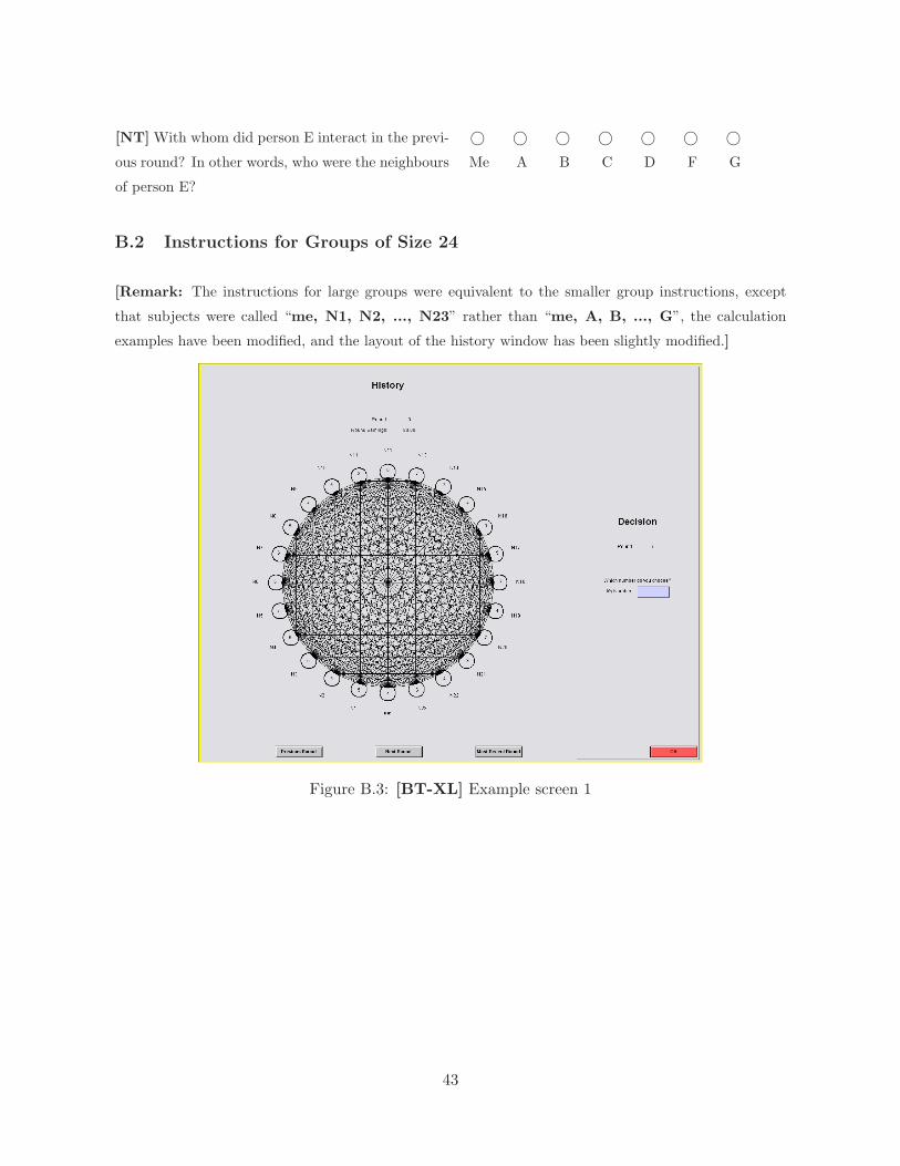
[NT] With whom did person E interact in the previ-

ous round? In other words, who were the neighbours

of person E?

©

Me

©

A

©

B

©

C

©

D

©

F

©

G

B.2 Instructions for Groups of Size 24

[Remark: The instructions for large groups were equivalent to the smaller group instructions, except

that subjects were called “me, N1, N2, ..., N23” rather than “me, A, B, ..., G”, the calculation

examples have been modified, and the layout of the history window has been slightly modified.]

Figure B.3: [BT-XL] Example screen 1

43

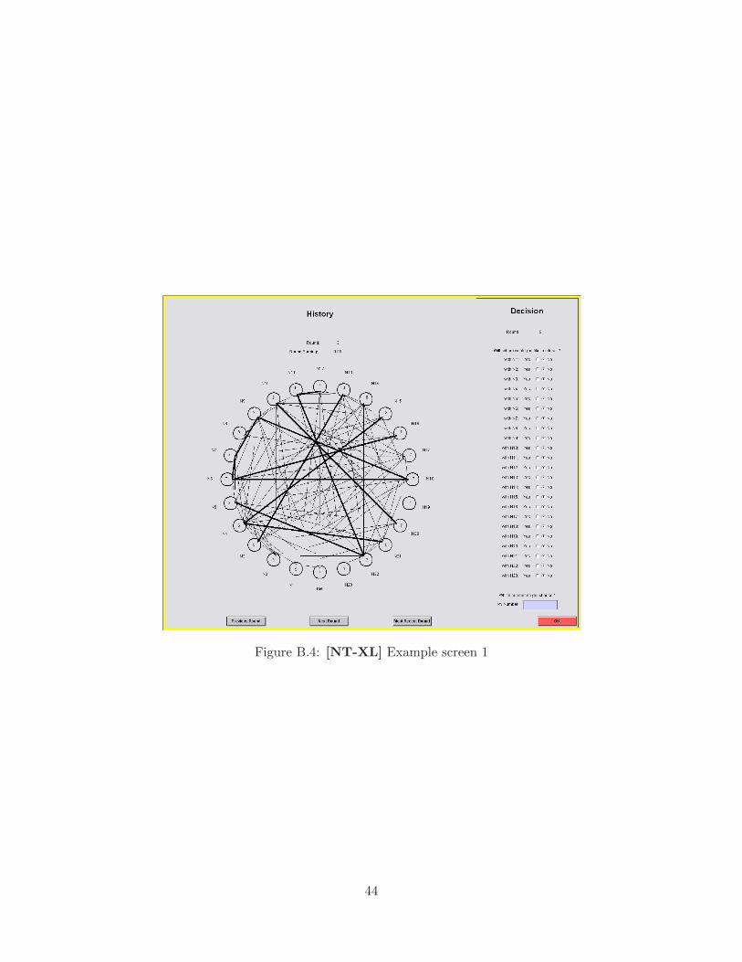
Figure B.4: [NT-XL] Example screen 1

44