Efficient and Targeted COVID-19 Border Testing via ...

of 14

Efficient and Targeted COVID-19 Border Testing via Reinforcement Learning

Hamsa Bastani*,1, Kimon Drakopoulos*,2,†, Vishal Gupta*,2, Jon Vlachogiannis3,

Christos Hadjicristodoulou4, Pagona Lagiou5, Gkikas Magiorkinis5, Dimitrios Paraskevis5, Sotirios Tsiodras6

1Department of Operations, Information and Decisions, Wharton School, University of Pennsylvania, Philadelphia, Pennsylvania, USA

2Department of Data Sciences and Operations, Marshall School of Business, University of Southern California, Los Angeles, California, USA

3AgentRisk, Los Angeles, California, USA 4Department of Hygiene and Epidemiology, University of Thessaly, Thessaly, Greece

5Department of Hygiene, Epidemiology and Medical Statistics, School of Medicine, National and Kapodistrian University of Athens, Athens, Greece

6 Department of Internal Medicine, Attikon University Hospital, Medical School, National and Kapodistrian University of Athens, Athens, Greece

*These authors contributed equally to this work † Corresponding author. Email: [email protected]

Throughout the COVID-19 pandemic, countries relied on a variety of ad-hoc border control protocols to allow for non-essential travel while safeguarding public health: from quarantining all travelers to restricting entry from select nations based on population-level epidemiological metrics such as cases, deaths or testing positivity rates [1, 2]. Here we report the design and performance of a reinforcement learning system, nicknamed “Eva.” In the summer of 2020, Eva was deployed across all Greek borders to limit the influx of asymptomatic travelers infected with SARS-CoV-2, and to inform border policies through real-time estimates of COVID-19 prevalence. In contrast to country-wide protocols, Eva allocated Greece’s limited testing resources based upon incoming travelers’ demographic information and testing results from previous travelers. By comparing Eva’s performance against modeled counterfactual scenarios, we show that Eva identified 1.85 times as many asymptomatic, infected travelers as random surveillance testing, with up to 2-4 times as many during peak travel, and 1.25-1.45 times as many asymptomatic, infected travelers as testing policies that only utilize epidemiological metrics. We demonstrate that this latter benefit arises, at least partially, because population-level epidemiological metrics had limited predictive value for the actual prevalence of SARS-CoV-2 among asymptomatic travelers and exhibited strong country-specific idiosyncrasies in the summer of 2020. Our results raise serious concerns on the effectiveness of country-agnostic internationally proposed border control policies [3] that are based on population-level epidemiological metrics. Instead, our work represents a successful example of the potential of reinforcement learning and real-time data for safeguarding public health.

of 14

Introduction In the first wave of the pandemic, many countries restricted non-essential travel to mitigate the spread of SARS-CoV-2. The restrictions crippled most tourist economies, with estimated losses of 1 trillion USD among European countries and 19 million jobs [3]. As conditions improved from April to July, countries sought to partially lift these restrictions, not only for tourists, but also for the flow of goods and labor. Different countries adopted different border screening protocols, typically based upon the origin country of the traveler. Despite their variety, we group the protocols used in early summer 2020 into 4 broad types:

• Allowing unrestricted travel from designated “white-list” countries. • Requiring travelers from designated “grey-listed” countries to provide proof of a negative RT-PCR test

before arrival. • Requiring all travelers from designated “red-listed” countries to quarantine upon arrival. • Forbidding any non-essential travel from designated “black-listed” countries.

Most nations employed a combination of all four strategies. However, the choice of which “color” to assign to a country differed across nations. For example, as of July 1st, 2020, Spain designated the countries specified in [1] as white-listed, Croatia designated these countries as grey-listed or red-listed. To the best of our knowledge, in all European nations except Greece, the above “color designations” were entirely based on population-level epidemiological metrics (e.g., see [1, 2]) such as cases per capita, deaths per capita, and/or positivity rates that were available in the public domain [4, 5, 6]. (An exception is the UK, which engaged in small-scale testing at select airports that may have informed their policies.) However such metrics are imperfect due to underreporting [7], symptomatic population biases [8, 9] and reporting delays. These drawbacks motivated our design and nation-wide deployment of Eva: the first fully algorithmic, real-time, reinforcement learning system for targeted COVID-19 screening with the dual goals of identifying asymptomatic, infected travelers and providing real-time information to policymakers for downstream decisions. The Eva System: Overview Eva as presented here was deployed across all 40 points of entry to Greece, including airports, land crossings, and seaports from August 6th to November 1st. Fig. 1 schematically illustrates its operation; Fig. 7 in Methods provides a more detailed schematic of Eva’s architecture and data flow. 1. Passenger Locator Form (PLF) All travelers must complete a PLF (one per household) at least 24 hours prior to arrival, containing (among other data) information on their origin country, demographics, point and date of entry. [10] describes the exact fields and how these sensitive data were handled securely. 2. Estimating Prevalence among Traveler Types We estimate traveler-specific COVID-19 prevalence using recent testing results from previous travelers through Eva. Prevalence estimation entailed two steps: First, we leverage LASSO regression from high-dimensional statistics [11] to adaptively extract a minimal set of discrete, interpretable traveler types based on their demographic features (country, region, age, gender); these types are updated on a weekly basis using recent testing results. Second, we use an empirical Bayes method to estimate each type’s prevalence daily. Empirical Bayes has previously been used in the epidemiological literature to estimate prevalence across many populations [12, 13]. In our setting, COVID-19 prevalence is generally low (e.g., ~2 in 1000), and arrival rates differ substantively

of 14

across countries. Combined, these features cause our testing data to be both imbalanced (few positive cases among those tested) and sparse (few arrivals from certain countries). Our empirical Bayes method seamlessly handles both challenges. Estimation details are provided in Section 2.2 of Methods.

Figure 1: Eva: A Reinforcement Learning System for COVID-19 Testing. Arriving passengers submit travel and demographic information 24 hours prior to arrival. Based on these data and testing results from previous passengers, Eva selects a subset of passengers to test. Selected passengers self-isolate for 24-48 hours while labs process samples. Positive passengers are then quarantined and contact tracing begins; negative passengers resume normal activities. Results are used to update Eva to improve future testing and maintain high-quality estimates of prevalence across traveler subpopulations.

3. Allocating Scarce Tests Leveraging these prevalence estimates, Eva targets a subset of travelers for (group) PCR testing upon arrival based solely on their type, but no other personal information. The Greek National COVID-19 Committee of Experts approved group (Dorfman) testing [14] in groups of 5 but eschewed larger groups and rapid testing due to concerns over testing accuracy. Eva’s targeting must respect various port-level budget and resource constraints that reflect Greece’s testing supply chain, which included 400 health workers staffing 40 points of entry, 32 laboratories across the country, and delivery logistics for biological samples. These constraints were (exogenously) defined and adjusted throughout the summer by the General Secretariat of Public Health. The testing allocation decision is entirely algorithmic and balances two objectives: First, given current information, Eva seeks to maximize the number of infected asymptomatic travelers identified (exploitation). Second, Eva strategically allocates some tests to traveler types for which it does not currently have precise estimates in order to better learn their prevalence (exploration). This is a crucial feedback step. Today’s allocations will determine the available data in Step 2 above when determining future prevalence estimates. Hence, if Eva simply (greedily) sought to allocate tests to types that currently had high prevalence, then, in a few days, it would not have any recent testing data about many other types that had moderate prevalence. Since COVID-19 prevalence can spike quickly and unexpectedly, this would leave a “blind spot” for the algorithm and pose a serious public health risk. Such allocation problems can be formulated as multi-armed bandits [15, 16, 17, 18] – which are widely studied within the reinforcement learning literature – and have been used in numerous

of 14

applications such as mobile health [19], clinical trial design [20], online advertising [21], and recommender systems [22]. Our application is a nonstationary [23, 24], contextual [25], batched bandit problem with delayed feedback [26, 27] and constraints [28]. Although these features have been studied in isolation, their combination and practical implementation poses unique challenges. One such challenge is accounting for information from “pipeline” tests (allocated tests whose results have not yet been returned); we introduce a novel algorithmic technique of certainty-equivalent updates to model information we expect to receive from these tests, allowing us to effectively balance exploration and exploitation in nonstationary, batched settings. To improve interpretability, we build on the optimistic gittins index for multi-armed bandits [29]; each type is associated with a deterministic index that represents its current “risk score”, incorporating both its estimated prevalence and uncertainty. Algorithm details are provided in Section 2.3 of Methods. 4. Grey-Listing Recommendations Eva’s prevalence estimates are also used to recommend particularly risky countries to be grey-listed, in conjunction with the Greek COVID-19 taskforce and the Presidency of the Government. Grey-listing a country entails a tradeoff: requiring a PCR test reduces the prevalence among incoming travelers, however, it also reduces non-essential travel significantly (approximately 39%, c.f. Sec. 5 of Methods), because of the relative difficulty/expense in obtaining PCR tests in summer 2020. Hence, Eva recommends grey-listing a country only when necessary to keep the daily flow of (uncaught) infected travelers at a sufficiently low level to avoid overwhelming contact-tracing teams [30]. Ten countries were grey-listed over the summer of 2020 (see Sec. 5 of Methods). Unlike testing decisions, our grey-listing decisions were not fully algorithmic, but instead involved human input. Indeed, while in theory, one might determine an “optimal” cut-off for grey-listing to balance infected arrivals and reduced travel, in practice it is difficult to elicit such preferences from decision-makers directly. Rather, they preferred to retain some flexibility in grey-listing to consider other factors in their decisions. 5. Closing the Loop Results from tests performed in Step 3 are logged within 24-48 hours, and then used to update the prevalence estimates in Step 2. To give a sense of scale, during peak season (August and September), Eva processed 41,830 (±12,784) PLFs each day, and 16.7% (± 4.8%) of arriving households were tested each day. Results Value of Targeted Testing: Cases Identified We first present the number of asymptomatic, infected travelers caught by Eva relative to random surveillance testing, i.e., where every arrival at a port of entry is equally likely to be tested. Random surveillance testing was Greece’s initial proposal and is very common, partly because it requires no information infrastructure to implement. However, we find that such an approach comes at a significant cost to performance (and therefore public health). We perform counterfactual analysis using inverse propensity weighting (IPW) [31, 32], which provides a model-agnostic, unbiased estimate of the performance of random testing.

of 14

Figure 2: Comparing Eva vs. Randomized Surveillance Testing. Infections caught by Eva (red) vs estimated number of cases caught by random surveillance testing (teal). The peak (resp. off-peak) season is Aug. 6 to Oct. 1 (resp. Oct. 1 to Nov. 1) and is denoted with triangular (resp. circular) markers. Seasons are separated by the dotted line. Solid lines denote cubic-spline smoothing with 95% confidence intervals in grey.

During the peak tourist season, we estimate that random surveillance testing would have identified 54.1% (±8.7%) of the infected travelers that Eva identified. (For anonymity, averages and standard deviations are scaled by a (fixed) constant, which we have taken without loss of generality to be the actual number of infections identified by Eva in the same period for ease of comparison.) In other words, to achieve the same effectiveness as Eva, random testing would have required 85% more tests at each point of entry, a substantive supply chain investment. In October, when arrival rates dropped, the relative performance of random testing improved to 73.4% (±11.0%) (see Fig. 2). This difference is largely explained by the changing relative scarcity of testing resources (see Fig. 3). As arrivals dropped, the fraction of arrivals tested increased, thereby reducing the value of targeted testing. Said differently, Eva’s targeting is most effective when tests are scarce. In the extreme case of testing 100% of arrivals, targeted testing offers no value since both random and targeted testing policies test everyone. See Sec. 3 of Methods for details.

Season

Peak

Improvement

Off−Peak

1.85x

1.36x

Sep Oct Nov

No.

Infe

ctio

ns C

augh

t (An

onym

ized)

of 14

Figure 3. Relative Efficacy of Eva over Random Surveillance vs. Fraction Tested. Ratio of number of infections caught by Eva relative to number of (estimated) infections caught by random surveillance testing, as a function of the fraction of tested travelers. Dotted (resp. dashed) line indicates the average fraction tested during the peak (resp. off-peak) tourist season. Triangular (circular) markers denote estimates from peak (off-peak) days. Solid blue line denotes cubic-spline smoothing with a 95% confidence interval in grey.

Value of Reinforcement Learning: Cases Identified We now compare to policies that require similar infrastructure as Eva, namely PLF data, but instead target testing based on population-level epidemiological metrics (e.g., as proposed by the EU [2]) rather than reinforcement learning. The financial investments of such approaches are similar to those of Eva, and we show these policies identify fewer cases. (Sec. 3.2.3 of Methods highlights additional drawbacks of these policies, including poor data reliability and a mismatch in prevalence between the general population and asymptomatic traveler population.) We consider three separate policies that test passengers with probability proportional to either (i) cases per capita, (ii) deaths per capita, or (iii) positivity rates for the passenger’s country of origin [4, 5, 6], while respecting port budgets and arrival constraints. We again use IPW to estimate counterfactual performance (see Fig. 4).

Season

Peak

Tested

Off−Peak

18.43%

31.01%

0x

2x

4x

20% 40% 60%Fraction Tested

Perfo

rman

ce R

atio

of 14

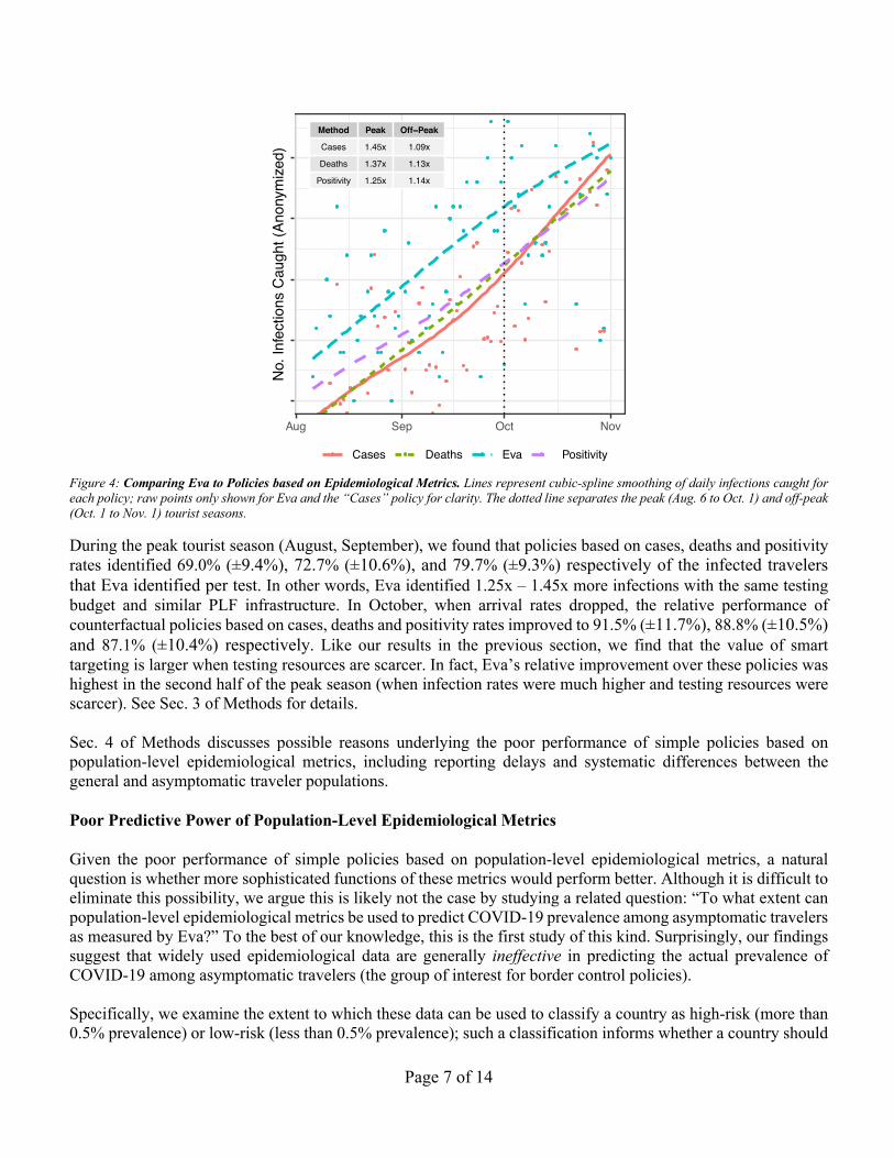
Figure 4: Comparing Eva to Policies based on Epidemiological Metrics. Lines represent cubic-spline smoothing of daily infections caught for each policy; raw points only shown for Eva and the “Cases” policy for clarity. The dotted line separates the peak (Aug. 6 to Oct. 1) and off-peak (Oct. 1 to Nov. 1) tourist seasons.

During the peak tourist season (August, September), we found that policies based on cases, deaths and positivity rates identified 69.0% (±9.4%), 72.7% (±10.6%), and 79.7% (±9.3%) respectively of the infected travelers that Eva identified per test. In other words, Eva identified 1.25x – 1.45x more infections with the same testing budget and similar PLF infrastructure. In October, when arrival rates dropped, the relative performance of counterfactual policies based on cases, deaths and positivity rates improved to 91.5% (±11.7%), 88.8% (±10.5%) and 87.1% (±10.4%) respectively. Like our results in the previous section, we find that the value of smart targeting is larger when testing resources are scarcer. In fact, Eva’s relative improvement over these policies was highest in the second half of the peak season (when infection rates were much higher and testing resources were scarcer). See Sec. 3 of Methods for details. Sec. 4 of Methods discusses possible reasons underlying the poor performance of simple policies based on population-level epidemiological metrics, including reporting delays and systematic differences between the general and asymptomatic traveler populations. Poor Predictive Power of Population-Level Epidemiological Metrics Given the poor performance of simple policies based on population-level epidemiological metrics, a natural question is whether more sophisticated functions of these metrics would perform better. Although it is difficult to eliminate this possibility, we argue this is likely not the case by studying a related question: “To what extent can population-level epidemiological metrics be used to predict COVID-19 prevalence among asymptomatic travelers as measured by Eva?” To the best of our knowledge, this is the first study of this kind. Surprisingly, our findings suggest that widely used epidemiological data are generally ineffective in predicting the actual prevalence of COVID-19 among asymptomatic travelers (the group of interest for border control policies). Specifically, we examine the extent to which these data can be used to classify a country as high-risk (more than 0.5% prevalence) or low-risk (less than 0.5% prevalence); such a classification informs whether a country should

Method

Cases

Peak

Deaths

Off−Peak

Positivity

1.45x

1.37x

1.25x

1.09x

1.13x

1.14x

Aug Sep Oct Nov

No.

Infe

ctio

ns C

augh

t (An

onym

ized)

Cases Deaths Eva Positivity

of 14

be grey- or black-listed. (A cutoff of 0.5% was typical for initiating grey-listing discussions with the Greek COVID-19 taskforce, but our results are qualitatively similar across a range of cutoffs.) We compute the true label for a country at each point in time based on Eva’s (real-time) estimates. We then train several models using a Gradient Boosted Machine (GBM) [33] on different subsets of covariates derived from the 14-day time series of cases per capita, deaths per capita, testing rates per capita, and testing positivity rates. Fig. 5 summarizes their predictive accuracy; we obtained similar results for other state-of-the art machine learning algorithms.

Figure 5: Predictive Power of Publicly Reported Epidemiological Metrics. Each of Models 1-4 uses a different subset of features from: 14-day time series of cases per capita, deaths per capita, tests performed per capita, and testing positivity rate. Model 5 additionally includes country fixed-effects to model country-level idiosyncratic behavior. Models 1-4 are essentially no better than random prediction, while Model 5 achieves slightly better performance. See Sec. 4.1 of Methods for details on model construction and features used in each model.

Note that a random model that uses no data has an AUROC of 0.5. Thus, Models 1-4 offer essentially no predictive value, suggesting that these population-level epidemiological data are not informative of prevalence among asymptomatic travelers. Model 5, which additionally uses country-level fixed effects, offers some improvement. These fixed effects collectively model country-specific idiosyncrasies representing aspects of their testing strategies, social distancing protocols and other non-pharmaceutical interventions that are unobserved in the public, epidemiological data. The improvements of Model 5 suggests that these unobserved drivers are critical to distinguishing high- and low-risk countries. Overall, this analysis not only raises concerns about travel protocols proposed by the EU [2] based solely upon widely used epidemiological metrics, but also about any protocol that treats all countries symmetrically. Indeed, the idiosyncratic effects of Model 5 suggest that the thresholds for deciding whether COVID-19 prevalence in travelers from Country A is spiking may differ significantly from that of Country B. See Section 4.1 for details. In Section 4.3 of Methods, we also study the information delay between a country’s publicly reported cases (the most common metric) and prevalence among asymptomatic travelers from that country. We expect a lag because

Model

1

AUROC

2

3

4

5

0.504

0.523

0.518

0.515

0.622

0.00

0.25

0.50

0.75

1.00

0.00 0.25 0.50 0.75 1.00False Positive Rate

True

Pos

itive

Rat

e

Model 1

Model 2

Model 3

Model 4

Model 5

of 14

of the time taken for symptoms to manifest, and reporting delays induced by poor infrastructure. We find a modal delay of 9 days. Value of Grey-Listing: Cases Prevented Eva’s measurements of COVID-19 prevalence were also used to provide early warnings for high-risk regions, in response to which Greece adjusted travel protocols by grey-listing these nations. We estimate that Eva prevented an additional 6.7% (±1.2%) infected travelers from entering the country through its early grey-listing decisions in the peak season; results in the off-peak season are similar. For privacy, we have expressed the benefit relative to the number of infected travelers identified by Eva. See Sec. 5 of Methods for details. Conclusions: Lessons Learned from Deployment and Design Principles To the best of our knowledge, Eva was the first large-scale data-driven system that was designed and deployed during the COVID-19 crisis. Leading up to and throughout deployment, we met twice a week with the COVID-19 Executive Committee of Greece, an interdisciplinary team of scientists and policymakers. Through those meetings, we gleaned several lessons that shaped Eva’s design and contributed to its success. Design the algorithm around data minimization. Data minimization (i.e., requesting the minimum required information for a task), is a fundamental tenet of data privacy and the General Data Protection Regulation (GDPR). We met with lawyers, epidemiologists, and policymakers before designing the algorithm to determine what data and granularity may legally and ethically be solicited by the PLF. Data minimization naturally entails a tradeoff between privacy and effectiveness. We limited requests to features thought to be predictive based on best available research at the time (origin, age and gender [34, 35]), but omitted potentially informative but invasive features (e.g., occupation). We further designed our empirical Bayes estimation strategy around these data limitations. Prioritize interpretability. For all parties to evaluate and trust the recommendations of a system, the system must provide transparent reasoning. An example from our deployment was the need to communicate the rationale for “exploration” tests, i.e., tests for types with moderate but very uncertain prevalence estimates). Such tests may seem wasteful. Our choice of empirical Bayes allowed us to easily communicate that types with large confidence intervals may have significantly higher risk than their point estimate suggests, and thus require some tests to resolve uncertainty; see, e.g., Figs. 9 and 11 in Methods, which were featured on policymakers’ dashboards. A second example was our choice to use gittins indices, which provide a simple, deterministic risk metric for each type that incorporates both estimated prevalence and corresponding uncertainty, driving intuitive test allocations. In contrast, using Upper Confidence Bound or Thompson Sampling with logistic regression [36, 37] would have made it more difficult to visualize uncertainty (a high-dimensional ellipsoid or posterior distribution) and test allocations would depend on this uncertainty through an opaque computation (a high-dimensional projection or stochastic sampling). This transparency fostered trust across ministries of the Greek Government using our estimates to inform downstream policy making, including targeting contact-tracing teams, staffing of mobile testing units, and adjusting social distancing measures. Design for flexibility. Finally, since these systems require substantial financial and technical investment, they need to be flexible to accommodate unexpected changes. We designed Eva in a modular manner disassociating type extraction, estimation, and test allocation. Consequently, one module can easily be updated without altering the

of 14

remaining modules. For example, had vaccine distribution begun summer 2020, we could define new types based on passengers’ vaccination status without altering our procedure for prevalence estimates or test allocation. Similarly, if rapid testing were approved, our allocation mechanism could be updated to neglect delayed feedback without affecting other components. This flexibility promotes longevity, since it is easier to get stakeholder buy-in for small adjustments to an existing system than for a substantively new approach.

Bibliography [1] Council recommendation on the temporary restriction on non-essential travel into the EU and the possible lifting of

such restriction, Brussels, 30 June 2020: https://www.consilium.europa.eu/media/47592/st_9208_2020_init_en.pdf. [2] Draft Council Recommendation on a coordinated approach to the restriction of free movement in response to the

COVID-19 pandemic, Brussels, 12 October 2020: General Secretariat of the Council. [3] "World Travel and Tourism Council," November 2020. [Online]. Available: Council

https://wttc.org/Research/Economic-Impact/Recovery-Scenarios. [4] J. Hasell, E. Mathieu, D. Beltekian, B. a. G. C. a. O.-O. E. Macdonald, M. Roser and H. Ritchie, "A cross-country

database of COVID-19 testing," Scientific data, vol. 7, no. 1, pp. 1-7, 2020. [5] M. Roser, H. Ritchie, E. Ortiz-Ospina and J. Hasell, "Coronavirus Pandemic (COVID-19)," OurWorldInData.org,

2020. [Online]. Available: https://ourworldindata.org/coronavirus. [6] E. Dong, H. Du and L. Gardner, "An interactive web-based dashboard to track COVID-19 in real time," The Lancet

infectious diseases, vol. 20, no. 5, pp. 533-534, 2020. [7] S. L. Wu, A. N. Mertens, Y. S. Crider, A. Nguyen, N. N. Pokpongkiat, S. Djajadi, A. Seth, M. S. Hsiang, J. M. J.

Colford, A. Reingold, B. F. Arnold, A. Hubbard and J. Benjamin-Chung, "Substantial underestimation of SARS-CoV-2 infection in the United States," Nature Communications, 2020.

[8] C. Muge, T. Matthew, L. Ollie, A. E. Maraolo, J. Schafers and H. Antonia, "SARS-CoV-2, SARS-CoV, and MERS-CoV viral load dynamics, duration of viral shedding, and infectiousness: a systematic review and meta-analysis," The Lancet Microbe, 2020.

[9] S. Phipps, Q. Grafton and T. Kompas, "Robust estimates of the true (population) infection rate for COVID-19: a backcasting approach," Royal Society Open Science, vol. 7, no. 11, 2020.

[10] Ministry of Civil Protection and Ministry of Tourism, Hellenic Republic, "Protocol for Arrivals in Greece," [Online]. Available: https://travel.gov.gr/#/policy.

[11] R. Tibshirani, "Regression shrinkage and selection via the lasso," Journal of the Royal Statistical Society: Series B (Methodological), pp. 267-288, 1996.

[12] S. Greenland and J. Robins, "Empirical-Bayes adjustments for multiple comparisons are sometimes useful," Epidemiology, pp. 244-251, 1991.

[13] O. J. Devine, T. Louis and E. Halloran, "Empirical Bayes methods for stabilizing incidence rates before mapping," Epidemiology, pp. 622-630, 1994.

[14] R. Dorfman, "The detection of defective members of large populations," The Annals of Mathematical Statistics, vol. 14, no. 4, pp. 436-440, 1943.

[15] W. Thompson, "On the likelihood that one unknown probability exceeds another in view of the evidence of two samples," Biometrika, pp. 285-294, 1933.

[16] T. L. Lai and H. Robbins, "Asymptotically efficient adaptive allocation rules," Advances in applied mathematics, pp. 4-22, 1985.

[17] J. Gittins, "Bandit processes and dynamic allocation indices," Journal of the Royal Statistical Society: Series B (Methodological), pp. 148-164, 1979.

of 14

[18] P. Auer, "Using confidence bounds for exploitation-exploration trade-offs," Journal of Machine Learning Research, pp. 397-422, 2002.

[19] A. Tewari and S. A. Murphy, "From Ads to Interventions: Contextual Bandits in Mobile Health," in Mobile Health, SpringerLink, 2017.

[20] A. Durand, C. Achilleos, D. Iacovides, K. Strati, G. D. Mitsis and J. Pineau, "Contextual bandits for adapting treatment in a mouse model of de novo carcinogenesis," in Machine Learning for Healthcare Conference, 2018.

[21] L. Li, W. Chu, J. Langford and R. Schapire, "A contextual-bandit approach to personalized news article recommendation," Proceedings of the 19th international conference on World wide web, pp. 6611-670, 2010.

[22] F. Amat, A. Chandrashekar, T. Jebara and J. Basilico, "Artwork personalization at Netflix," Proceedings of the 12th ACM conference on recommender systems, pp. 487-488, 2018.

[23] O. Besbes, Y. Gur and A. Zeevi, "Stochastic multi-armed-bandit problem with non-stationary rewards," Advances in neural information processing systems, pp. 199-207, 2014.

[24] H. Luo, C.-Y. Wei, A. Agarwal and J. Langford, "Efficient contextual bandits in non-stationary worlds," Conference on Learning Theory, pp. 1739-1776, 2018.

[25] H. Bastani and M. Bayati, "Online decision making with high-dimensional covariates," Operations Research, pp. 276-294, 2020.

[26] Z. Gao, Y. Han, Z. Ren and Z. Zhou, "Batched multi-armed bandits problem," Advances in Neural Information Processing Systems, pp. 503-514, 2019.

[27] V. Perchet, P. Rigollet, S. Chassang and E. Snowberg, "Batched bandit problems," The Annals of Statistics, pp. 660-681, 2016.

[28] S. Agrawal and N. Devanur, "Bandits with concave rewards and convex knapsacks," Proceedings of the fifteenth ACM conference on Economics and computation, pp. 989-1006, 2014.

[29] E. Gutin and V. Farias, "Optimistic gittins indices," Advances in Neural Information Processing Systems, pp. 3153-3161, 2016.

[30] Hellewell, J.; Abbott, S.; Gimma, A.; Bosse, N. I.; Jarvis, C. I.; Russell, T. W.; Munday, J. D.; Kucharski, A. J.; Edmunds, W. J.; Centre for the Mathematical Modelling of Infectious Diseases COVID-19 Working Group; Funk, S.; Eggo, R. M., "Feasibility of controlling COVID-19 outbreaks by isolation of cases and contacts," The Lancet. Global health, 2020.

[31] W. G. Imbens and B. D. Rubin, Causal Inference in Statistics, Social and Biomedical Sciences, Cambridge University Press, 2015.

[32] P. Rosenbaum and D. Rubin, "The central role of the propensity score in observational studies for causal effects," Biometrika, vol. 70, no. 1, pp. 41-55, 1983.

[33] Friedman, "Greedy function approximation: a gradient boosting machine," Annals of Statistics, pp. 1189-1232, 2001. [34] N. Davies, P. Klepac and Y. Liu et al., "Age-dependent effects in the transmission and control of COVID-19

epidemics," Nature Medicine, 2020. [35] S. Davies and B. Bennet, "A gendered human rights analysis of Ebola and Zika: Locating gender in global health

emergencies," International Affairs. [36] S. Agrawal and N. Goyal, "Thompson sampling for contextual bandits with linear payoffs," in International

Conference on Machine Learning, 2013. [37] W. Chu, L. Li, L. Reyzin and R. Schapire, "Contextual bandits with linear payoff functions," in Conference on

Artificial Intelligence and Statistics, 2011.

of 14

End Notes Acknowledgements. The authors would like to thank all members of the Greek COVID-19 Taskforce, the Greek Prime Minister Kyriakos Mitsotakis, the Ministry of Digital Governance, the General Secretariat for Civil Protection, the Ministry of Health, the National Public Health Organization, the development team from Cytech as well as the border control agents, doctors, nurses and lab personnel that contributed to Eva’s deployment. Furthermore, the authors would like to thank Osbert Bastani for discussions and analysis on constructing custom risk metrics from public data. V.G. was partially supported by the National Science Foundation through NSF Grant CMMI-1661732. We also thank the Editor and 4 anonymous reviewers for their comments on an earlier draft of this manuscript.

Author Contributions. H.B., K.D., and V.G. constructed the model, designed and coded the algorithm, and performed the analysis in this paper. J.V. designed the software architecture and APIs to communicate with the Central Database of the Ministry of Digital Governance. C.H., P.L., G.M., D.P., and S.T. contributed to and informed epidemiological modeling choices of the system. All authors coordinated Eva’s operations and logistics throughout its deployment.

Author Information. H.B., V.G., and J.V. declare no conflict of interest. K.D. declares non-financial competing interest as an unpaid Data Science and Operations Advisor to the Greek Government from May 1st, 2020 to Nov 1st, 2020. C.H., P.L., G.M., D.P., and S.T. declare non-financial competing interest as members of the Greek National COVID-19 Taskforce. Correspondence should be addressed to [email protected].

of 14

Data and Code Availability Data availability. To support further research, aggregated, anonymized data are available at https://github.com/kimondr/EVA_Public_Data. These data aggregate passenger arrival and testing information over pairs of consecutive days, country of origin, and point of entry. The finer granularity data that support the (exact) findings of this study are protected by GDPR. These data are available from the Greek Ministry of Civil Protection but restrictions apply to the availability of these data, which were used under license for the current study, and so are not publicly available. Access to these data can only be granted by the Greek Ministry of Civil Protection ([email protected]) for research that is conducted in the public interest for public health (GDPR Recital 159) and scientific purposes (GDPR Article 89). Finally, the population-level epidemiological metrics used in our analysis can be obtained freely from the “Our World In Data COVID-19 dataset (https://github.com/owid/covid-19-data/tree/master/public/data). Code Availability. All code used in this paper was written in a combination of R and Python 3.7 The code for the deployment of the algorithm on a sample dataset is available at https://github.com/vgupta1/EvaTargetedCovid19Testing. The code for reproducing the results of our counterfactual analysis is available at https://github.com/vgupta1/Eva_CounterfactualAnalysis.

of 32

Methods

1 Problem Description Notation and System Constraints Let 𝑡 ∈ {1, … , 𝒯} index time (in days), 𝑒 ∈ {1,… , ℰ} index points of entry, and 𝑐 ∈ {1,… , 𝒞} index the set of 193 countries from which travelers may originate. Moreover, for each point of entry𝑒, let 𝐵!(𝑡) denote the budget of available tests at time 𝑡. Pertinent demographic data about a passenger (extracted from their PLF) include their country and region of origin, age group and gender. Since all extracted features are categorical, we represent them with a finite, discrete set of values 𝒳. We refer to passengers with features 𝑥 ∈ 𝒳 as 𝑥-passengers. Let 𝐴"!(𝑡) denote the number of 𝑥-passengers arriving with date of entry 𝑡 and point of entry 𝑒. For every 𝑥 ∈ 𝒳, let 𝑅"(𝑡) denote the unknown, time-varying, underlying prevalence among 𝑥-passengers, i.e., the probability that a 𝑥-passenger is infected. The budgets 𝐵!(𝑡) were exogenously determined by the Secretary General of Public Health. Note that the availability of tests relative to arrivals varies significantly across points of entry (see Fig. 6). Decision Problem The primary decision problem on day 𝑡 is to choose the number of tests 𝑇"!(𝑡) to allocate to 𝑥-passengers at point of entry 𝑒. To formally define this problem, we first specify the information available at time 𝑡. Namely, let 𝑃"(𝑡) and 𝑁"(𝑡) denote the number of 𝑥-passengers that tested positive and negative at time 𝑡, respectively. Then, since labs take up to two days to process testing results, the available information on day 𝑡 is

{𝑃"(𝑡#), 𝑁"(𝑡#)}"∈𝒳,(!)(*+.

Thus, at the beginning of day 𝑡, we must determine the number of tests 𝑇"!(𝑡) to be performed on 𝑥-passengers at point of entry 𝑒 using this information. Furthermore, our testing decisions need to satisfy two constraints:

∑ 𝑇"!(𝑡)"∈𝒳 ≤ 𝐵!(𝑡), ∀𝑒 ∈ {1, … , ℰ}, (Budget Constraint),

ensuring that the number of allocated tests does not exceed the budget at each point of entry, and

𝑇"!(𝑡) ≤ 𝐴"!(𝑡), ∀𝑥 ∈ 𝒳, 𝑒 ∈ {1, … , ℰ},(Arrivals Constraint),

ensuring that the number of allocated tests for 𝑥-passengers does not exceed the number of arriving 𝑥-passengers. A secondary decision problem is to choose “color designations” for every country as described in the main text. We denote the set of black, grey, and white-listed countries at time 𝑡 by ℬ( , 𝒢( ,𝒲(, respectively. Note that determining these sets must be done one week in advance (to provide notice to travelers of possibly changing travel requirements). Hence the relevant sets to choose at time 𝑡 are ℬ(,-, 𝒢(,-,𝒲(,-.

of 32

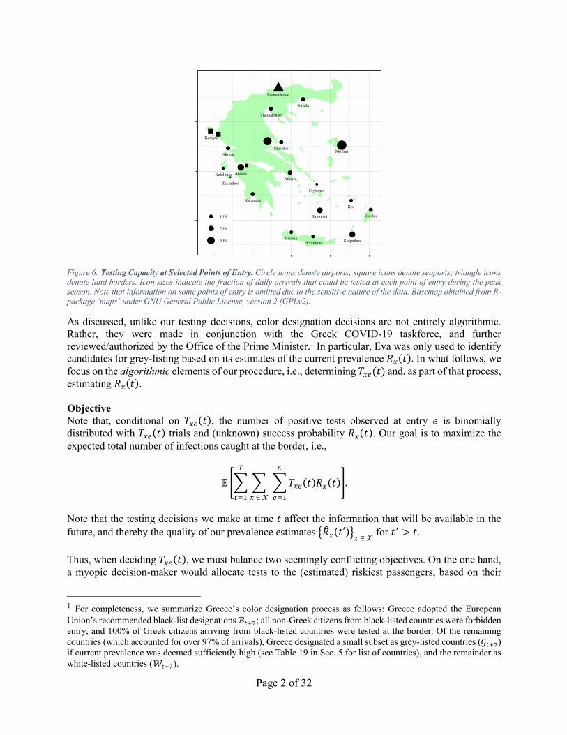
Figure 6: Testing Capacity at Selected Points of Entry. Circle icons denote airports; square icons denote seaports; triangle icons denote land borders. Icon sizes indicate the fraction of daily arrivals that could be tested at each point of entry during the peak season. Note that information on some points of entry is omitted due to the sensitive nature of the data. Basemap obtained from R-package ‘maps’ under GNU General Public License, version 2 (GPLv2).

As discussed, unlike our testing decisions, color designation decisions are not entirely algorithmic. Rather, they were made in conjunction with the Greek COVID-19 taskforce, and further reviewed/authorized by the Office of the Prime Minister.1 In particular, Eva was only used to identify candidates for grey-listing based on its estimates of the current prevalence 𝑅"(𝑡). In what follows, we focus on the algorithmic elements of our procedure, i.e., determining 𝑇"!(𝑡) and, as part of that process, estimating 𝑅"(𝑡). Objective Note that, conditional on 𝑇"!(𝑡), the number of positive tests observed at entry 𝑒 is binomially distributed with 𝑇"!(𝑡) trials and (unknown) success probability 𝑅"(𝑡). Our goal is to maximize the expected total number of infections caught at the border, i.e.,

𝔼 @A A A𝑇"!(𝑡)𝑅"(𝑡)ℰ

!/0"∈𝒳

𝒯

(/0

B.

Note that the testing decisions we make at time 𝑡 affect the information that will be available in the future, and thereby the quality of our prevalence estimates C𝑅D"(𝑡′)F"∈𝒳 for 𝑡# > 𝑡. Thus, when deciding 𝑇"!(𝑡), we must balance two seemingly conflicting objectives. On the one hand, a myopic decision-maker would allocate tests to the (estimated) riskiest passengers, based on their

1 For completeness, we summarize Greece’s color designation process as follows: Greece adopted the European Union’s recommended black-list designations ℬ!"#; all non-Greek citizens from black-listed countries were forbidden entry, and 100% of Greek citizens arriving from black-listed countries were tested at the border. Of the remaining countries (which accounted for over 97% of arrivals), Greece designated a small subset as grey-listed countries (𝒢!"#) if current prevalence was deemed sufficiently high (see Table 19 in Sec. 5 for list of countries), and the remainder as white-listed countries (𝒲!"#).

Promachonas

Rhodes

Karpathos

Mykonos

Santorini

Athens

Kerkyra

Kos

Zakinthos

Kefalonia

Aktion

Araxos

Skiathos

HeraklionChania

Thessaloniki

Kavala

Kalamata

Mitilini

10%

20%

50%

of 32

features 𝑥 and our current prevalence estimates C𝑅D"(𝑡)F. On the other hand, a forward-looking decision-maker would want to collect data on 𝑥-passengers for every value of 𝑥, in order to make accurate future assessments on which passengers are risky. This suggests allocating tests uniformly across feature realizations to develop high-quality surveillance estimates. This tension – known as the exploration-exploitation tradeoff – is well-studied in the multi-armed bandit literature [1, 2, 3]. Optimal solutions balance the need to explore (accurately learn the current prevalence 𝑅"(𝑡) for all 𝑥) and to exploit (use the estimated prevalence C𝑅D"(𝑡)F"∈𝒳 to allocate tests to the riskiest passengers).

2 Algorithm Description 2.1 Overview of Algorithm The tradeoff presented in Section 1 resembles a multi-armed bandit problem. However, our setting exhibits a number of salient features that distinguish it from the classical formulation:

1. Non-stationarity: The prevalence 𝑅"(𝑡) is time-varying. 2. Imbalanced Data: On average, only 2 in 1000 passengers tests positive, meaning the data

{𝑃"(𝑡#), 𝑁"(𝑡#)}"∈𝒳,(!)(*+ is very imbalanced with mostly negative tests. 3. High-Dimensionality: The number of possible features 𝒳 is very large. 4. Batched decision-making: All testing allocations for a day must be determined at the start of

the day (batch) for each point of entry. 5. Delayed Feedback: Labs may take up to 48 hours to return testing results. 6. Constraints: Each point of entry is subject to its own testing budget and arrival mix.

Although these features have been studied in isolation, their combination poses unique challenges. We next propose a novel algorithm that addresses these features in our setting. We separate our presentation into two parts: estimation and allocation. Our estimation procedure (Section 2.2) builds on ideas from empirical Bayes and high-dimensional statistics to address the challenges of non-stationarity, imbalanced data and high-dimensionality. Our allocation procedure (Section 2.3) uses these estimates and adapts classical multi-arm bandit algorithms to address the challenges of batched decision-making, delayed feedback, and budget constraints. Before delving into details, we note that to address the aforementioned high-dimensionality, we periodically partition the set of features 𝒳 into types, denoted by 𝐾(. On first reading the reader can take a passenger’s type to be equivalent to their country of origin (i.e., ignoring more granular feature information such as origin region, age and gender) without much loss of meaning. However, in reality, we distinguish particularly risky passenger profiles within a country as additional, distinct types, where these “risky profiles” are identified dynamically using LASSO regression with recent testing results (see Section 2.2 for details). Over time, as new testing data arrives, we update this partition, yielding a time-dependent set of types 𝐾(. We treat all 𝑥-passengers of the same type 𝑘 ∈ 𝐾( symmetrically in our estimation and allocation procedures, i.e., our estimates satisfy �̂�""(𝑡) = �̂�"#(𝑡) for all features 𝑥0, 𝑥+ ∈ 𝑘. This process reduces the dimensionality of our estimation and allocation problems from |𝒳| to |𝐾(|.

of 32

Fig. 7 overviews the architecture and data flow of Eva.

Figure 7: The Data Flow of Eva. The core algorithmic components of Eva are depicted by shaded boxes. All data flows, including personal data obtained via the PLF, were managed by the Greek Government (see [4]). Adaptive types were updated once per week and held constant between updates. Throughout the summer, our algorithm only identified adaptive types based on the country and region; types were never defined based on age group and gender (see also Section 2.2 below).

2.2 Estimation In this section, we focus on developing estimates for prevalence rates 𝑅2(𝑡) for a given day 𝑡; we drop the time index when it is clear from context. Recall that the (unknown) prevalence rates 𝑅2(𝑡) are time-varying. Common strategies for estimation in time-varying settings include discarding sufficiently old data [5, 6] or exponential smoothing [7]. The kernel smoothing literature [8] suggests that discarding old data might be preferred if the rates 𝑅2(𝑡) are particularly non-smooth in time. Based on this intuition and conversations with epidemiologists on Greece’s COVID-19 taskforce, we choose to discard testing results that are more than 16 days old. As before, let

𝑃2 = A 𝑃2(𝑡#)(*3

(!/(*04

,

denote the total number of type 𝑘 passengers that tested positive over the past 14 days of test results, and let

𝑁2 = A 𝑁2(𝑡#)(*3

(!/(*04

,

denote the total number of type 𝑘 passengers that tested negative over the past 14 days of test results. An unbiased, and natural estimate of the prevalence for type 𝑘 is

�̂�25678! =𝑃2

𝑃2 +𝑁2. (1)

of 32

However, because prevalence rates are low (on the order of 2 in a 1000), the variability of this estimator is on the same order as 𝑅2(𝑡) for moderate values of 𝑇2!(𝑡). Worse, for rare types where 𝑇2!(𝑡) is necessarily small (e.g., less than 100 arrivals in last 16 days), the variability is quite large. This high variability often renders the estimator unstable/inaccurate, an observation also recognized by prior epidemiological literature [9, 10]. As a simple illustration, consider a (foolish) baseline estimator that estimates every prevalence to be zero. We compute this baseline estimator and the naïve estimator in Eq. (1) for all countries as of September 1, 2020. We find that the average MSE (averaged over countries) of the naïve estimator is larger than that of the baseline estimator (see Fig. 8 below). In fact, a conservative estimate of the error of �̂�25678! is

OExcessMSEof�̂�25678! overBaseline = √. 000334 = 0.018,

which is larger than the typical prevalence of most countries. In other words, any potential signal is entirely washed out by noise.

Figure 8: Excess MSE over Baseline Estimator. The baseline estimates zero prevalence for all types. The naïve estimator (clipped from the plot for readability) corresponds to a prior strength of zero and has far worse MSE than the baseline. Our empirical Bayes estimator (red dot) substantively improves performance and approximately minimizes MSE by trading off bias and variance. To compensate for high variability and potentially rare types, we adopt an empirical Bayes perspective. This improves the stability of our estimates at the expense of introducing some bias. Our approach naturally allows information-sharing across types, so that rare types partially borrow data from other similar types to improve their stability. At a high level, our estimation procedure has two steps: First, for each color designation (white, grey or black-listed) 𝑙 ∈ {𝒲(,𝒢( , 𝔅(}, we fit a prior Beta(α9(𝑡), β9(𝑡)) for all types from countries of that color-designation. Second, we compute Bayesian (posterior) estimates for each 𝑅2(𝑡), assuming 𝑅2(𝑡) was drawn from the appropriately colored prior. Specifically, consider countries of color 𝑙 ∈ {𝒲(,𝒢( , 𝔅(}, and the corresponding set of types ℒ9 = {𝑘 ∈𝐾( ∶ 𝑘is from a country in l}. Let 𝑇2 = 𝑃2 +𝑁2 be the total number of tests (with results) allocated to

0.00000

0.00004

0.00008

0.00012

0 100 200 300 400 500Prior Strength (α + β)

Exce

ss M

SE

of 32

type 𝑘 over the last 16 days. Conditional on 𝑇2, 𝑃2 is approximately binomially distributed with 𝑇2 trials and success probability 𝑅2. If we further assume that for each 𝑘 ∈ ℒ9, 𝑅2 was drawn independently from a Beta(𝛼:, β9) distribution, then the strong law of large numbers yields:

1|ℒ9|

A 𝑃2𝑇22∈ℒ$

6.=.mn

1|ℒ9|

A 𝔼 o𝑃2𝑇2 |𝑇2p

2∈ℒ$

= 1|ℒ9|

A 𝔼[𝑅2] = 𝛼9

𝛼9 +𝛽92∈ℒ$

and 1|ℒ9|

A 𝑃2(𝑃2 − 1)𝑇2(𝑇2 − 1)2∈ℒ$

6.=.mn

1|ℒ9|

A 𝔼 u𝑃2(𝑃2 − 1)𝑇2(𝑇2 − 1)

|𝑇2v2∈ℒ$

=1|ℒ9|

A 𝔼[𝑅2+] = 𝛼l+

(𝛼l +𝛽l)++

𝛼l 𝛽l(𝛼l +𝛽9)+(𝛼l +𝛽l + 1)2∈ℒ$

,

where the limits are taken as |ℒ9| → ∞. Taking the left sides of the above two expressions as estimators for the right sides, we can rearrange to find estimates of (α9 , β9), yielding

αy: =𝑀09+ (1 − 𝑀09)𝑀+9+ −𝑀09

+ −𝑀09

βD : = αy:(1 − 𝑀09)𝑀09

𝑀09 =1|ℒ9|

A 𝑃2𝑇22∈ℒ$

(2)

𝑀+9 =1|ℒ9|

A 𝑃2(𝑃2 − 1)𝑇2(𝑇2 − 1)2∈ℒ$

(3)

We repeat this procedure separately for each of the three-color designations. Equipped with these priors, we then compute posterior distributions for each type 𝑘 ∈ ℒ9. By conjugacy, these areBeta(α>, β>)distributedwith estimates

αy2 =αy9 + P2and𝛽�2 = 𝛽�9 +𝑁2, suggesting the following empirical Bayes estimate of the prevalence 𝑅2:

�̂�2?@ =αy2

αy2 + 𝛽�2. (4)

To provide intuition, notice that if type 𝑘 comes from a country with color designation 𝑙, our posterior estimate can be rewritten as

�̂�2?@ = �1 −𝑇2

𝑇2 + 𝛼9 +𝛽9�

α9α9 + 𝛽9

+𝑇2

𝑇2 + 𝛼9 +𝛽9�̂�25678! ,

i.e., it is a weighted average between the naïve prevalence estimator and our prior mean. The sum (α9 + 𝛽9) is often called the strength of the prior. For rare types where 𝑇2 is small relative to (α9 + 𝛽9), the estimator is close to the prior mean (i.e., it draws information from similar types). For common types where 𝑇2 is large relative to (α9 + 𝛽9), it is close to the naïve estimator (i.e., it lets the type’s own testing data speak for itself). This structure matches our intuition that the naive estimator should only be used when 𝑇2 is large enough.

of 32

Below, we summarize the estimation strategy. Subroutine 1: Estimating Prevalence via Empirical Bayes Input: # of positives 𝑃2, negatives 𝑁2 and tests 𝑇2 for each type 𝑘 in the past 14 days of test results.

for each color designation of countries 𝑙 ∈ {𝒲(,𝒢( , 𝔅(} Compute 𝑀09 , 𝑀+9 from Eq. (2) and (3)

αy9 ←𝑀09+ (1 − 𝑀09)𝑀+9+ −𝑀09

+ −𝑀09 , βD 9 ← αy9(1 − 𝑀09)𝑀09

for all types 𝑘 ∈ ℒ9 whose origin country is in 𝑙: αy2 ← αy9 + 𝑃2 and 𝛽�2 ←βD9 +𝑁2

end

end

Fig. 8 shows the excess MSE for various estimators with differing strength in the prior (the naïve estimator �̂�25678! corresponds to a prior strength of zero and its MSE is too large to fit on the plot). Our moment-matching estimator (red dot) approximately minimizes the MSE while maintaining a tractable closed-form expression. 2.2.1 Reducing Dimensionality through Adaptive Type Extraction As mentioned earlier, we adaptively partition the discrete space of features 𝒳 into a smaller set of types 𝐾( to reduce the dimensionality of the problem. Defining types entirely by a passenger’s country of origin is attractive for its operational simplicity and because geography is highly predictive of prevalence. That said, there can be significant heterogeneity in infection prevalence based on other passenger feature information. For example, certain regions within a country may have a high population density and low social distancing compliance relative to the rest of the country, resulting in a much higher risk for passengers originating from that region; certain age brackets or genders may also carry higher risk. Defining types solely at the country-level risks poor test allocations by failing to test passengers with features that suggest high risk. Consequently, our dimensionality reduction procedure starts with types defined at the country level, but then goes one step further to distinguish particularly risky passengers based on their feature information (origin region and demographic characteristics) as additional, distinct types.2 These additional types are identified dynamically based on recent testing results and allow us to exploit intra-country heterogeneity in prevalence to better allocate testing resources. We identify additional types using the celebrated LASSO procedure [11], which has also previously been used for dimensionality reduction in contextual bandits [12]. Specifically, we first apply our previous empirical Bayes estimation strategy assuming country-based types. Given these estimates, we then perform a LASSO logistic regression on the last 14 days of testing results, where the unit of observation is a single passenger’s test, and features include (1) the estimated prevalence �̂�2?@ of the

2 Regions indicates more granular locations within a country (e.g., state or province). Since different countries use different nomenclature, we use the generic term “region.”

of 32

passenger’s origin country (estimated in previous step), (2) indicator variables for potential regions, (3) indicator variables for gender-country pairs and (4) indicator variables for age-country pairs. As will become clear below, we interact gender and age with the country of origin since our goal is to further split existing country-level types based on demographic information, as warranted by the data. Mathematically, let 𝑖 denote a tested passenger (from the last 14 days of testing results), 𝑦7 ∈ {0, 1} denote their binary test result, 𝑐7 denote their origin country, 𝑓7 denote their origin region, 𝑔7 denote their gender-country pair (i.e., the cross product of their gender and country categorical variables), and 𝑎7 denote their age-country pair (i.e., the cross product of their age group and country categorical variables). We then perform the LASSO logistic regression:

𝑦7 = 𝛿A�̂�A%?@ +A𝛿B𝟏{𝑓 = 𝑓7}

B

+A𝛿C𝟏{𝑔 = 𝑔7}C

+A𝛿6𝟏{𝑎 = 𝑎7}6

+𝜖7 (5)

Let the number of unique countries from the last two weeks be 𝐶, the number of unique regions from the last two weeks be 𝑈, and further note that there are 3 gender options and 10 possible age brackets. Then, the total number of features is 1 + 13𝐶 + 𝑈. Note that 𝐶 and 𝑈 change over time as a function of the types of recent arrivals; we typically had scheduled arrivals from 𝐶 ≈ 170 countries and roughly 𝑈 ≈ 17,000 cities. The regression above yields a sparse vector of coefficients �𝛿�A , 𝛿�B , 𝛿�C, 𝛿�6�. These coefficients indicate types of passengers whose estimated prevalence (based on their feature information) is notably different than their estimated prevalence based solely on their origin country, based on recent testing data. We are primarily interested in identifying risky passenger types (so we can concentrate our limited testing resources on such passengers). Hence, we only introduce new type(s) when we identify positive coefficients in the support. As a clarifying example, if a region 𝑓 has a corresponding positive 𝛿�B, then the prevalence of passengers from region 𝑓 have notably higher prevalence than passengers of its corresponding country 𝑐. Thus, we define a new type for passengers originating from 𝑓, but also retain a type for passengers originating from 𝑐 that are not from 𝑓. We apply similar transformations for other positive coefficients in the LASSO regression as well. Interestingly, during the summer of 2020, we always found that 𝛿�C = 0 for all gender-country pairs and 𝛿�6 = 0 for all age-country pairs, i.e., we never found the age bracket and/or gender to be predictive of passenger test results beyond country/region of origin. This non-predictive behavior is likely because only one member of a household fills out the PLF (using their own age and gender) but the household likely spans members of different ages and genders. Note that the constraint of one PLF per household was a hard constraint imposed by Greek government. The process is summarized below in Subroutine 2. For simplicity, we have only stated the algorithm in the case of potentially positive elements in 𝛿�B, since we never found other features to be predictive. Subroutine 2: Adaptive Type Extraction

Input: 𝑦7 , 𝑐7 , 𝑓7 # historical test results with country and region dummies

Perform Lasso regression according to Eq. (5) return set of types 𝐾( = {1, … , 𝐶} ∪ �𝑓7:�𝛿�B�7 > 0�

of 32

We re-ran this procedure every week to obtain new types 𝐾(, which are used daily for empirical Bayes estimation of prevalence rates as well as the bandit allocation algorithm. Fig. 9 shows the resulting (anonymized) prevalence and confidence intervals for a typical day (batch) from the summer of 2020. The x-axis indexes different types ordered from highest prevalence (left) to lowest prevalence (right). This plot was featured on the dashboards of policy-makers in the Greek government to communicate the status of the pandemic and to inform grey-listing decisions.

Figure 9: Estimated Prevalence by Type. Shown for each type on a given day (batch). Types are ordered from high to low risk. Center points are our empirical Bayes estimates of prevalence (mean of estimated posterior distribution). Confidence intervals correspond to the 5% and 95% quantiles of estimated posterior distribution. Note that the ability to shrink a confidence interval via targeted exploration is limited by the number of arrivals of that type. Estimates formed from n = 64,161 passengers tested in previous 14 days.

2.3 Allocating Test Results 2.3.1 Optimistic Gittins Indices Online optimization problems and the aforementioned exploration-exploitation tradeoff have been studied in the literature since the seminal work of [2, 1]. In the classical setting, the celebrated Gittins index theorem provides the optimal dynamic solution to this tradeoff [3], but it is typically intractable to compute this solution exactly. Consequently, various heuristics with near-optimal asymptotic performance guarantees such as Upper Confidence Bound [13], Thompson Sampling [2] and optimistic gittins indices [14] have been proposed to overcome these issues. Our approach builds upon the optimistic gittins index of [14]. We first describe the mechanics of the optimistic gittins index in a classical setting, and then describe how we adapt this technique to address the unique combination of challenges in our setting – batched decision-making, delayed feedback and port-specific budget/arrival constraints. Recall that our estimation procedure yields a Beta posterior distribution with parameters 𝛼2 , 𝛽2 for type 𝑘. Let 𝐹D,E be the CDF of a Beta distribution with parameters 𝛼 and 𝛽. Then, from [14], the optimistic gittins index 𝜆2 for type 𝑘 (with a 1-step lookahead window and a discount factor 𝛾) is the unique solution to the following equation:

𝜆2 =𝛼2

𝛼2 + 𝛽2�1 − 𝛾𝐹D&,0,E&(𝜆2)� + 𝛾𝜆2 �1 − 𝐹D&,E&(𝜆2)� . (6)

Country/City (Anonymized)

Prev

alen

ce (%

) (An

onym

ized)

of 32

In the classical setting, the optimistic gittins index algorithm proceeds very simply: (1) test the type (arm) with the highest index, (2) observe the resulting (immediate) feedback and use it to update the posterior for that type, (3) calculate the new index for that type, and (4) repeat. Importantly, one can confirm that Eq. (6) naturally balances the twin goals of exploration (prioritizing types with a wide prior, i.e., large variance) and exploitation (prioritizing types with large, estimated prevalence �̂�2?@). 2.3.2 Challenges with the Conventional Optimistic Gittins Index Algorithm Unfortunately, this approach does not perform well in our setting because we do not observe immediate feedback from our tests. Rather, we choose thousands of passengers to test in a given day (avg: 5300; std dev: 998) and receive no feedback on these allocations for 48 hours. Applied naively, the algorithm would simply keep testing the same type (the one with the highest initial index) repeatedly because the computed indices for each type remain the same throughout a given batch (day). Such an outcome is clearly undesirable. The batched bandit literature [15, 16] partially resolves this issue in stationary environments by uniformly exploring all types in early batches, and then committing to the type with the highest prevalence in later exploitation batches. However, this strategy is untenable in highly non-stationary environments, because the data from initial exploration in early batches are not representative of current rates (recall that we only use the last 14 days of test results for estimation), i.e., we must continuously explore and collect new data on each type to form accurate prevalence estimates. Thus, it is critical in our setting that our allocation policy combine exploration and exploitation within a batch. Relatedly, at the start of each batch, we also have a large number of tests that are already in the “pipeline” (i.e., tests that have been conducted but the results have not yet been received from the labs) from the past 2 days. A good policy should also account for the expected information that will be imbued by these pipeline tests when making new allocations. 2.3.3 Certainty Equivalent Pseudo-Updating In order to address the delayed-feedback and batching challenges above, we propose certainty-equivalent pseudo-updates to our indices during the course of the allocation assignment algorithm. These updates do not alter the mean estimates of prevalence but reduce the variance of our estimates based on the number of tests allocated thus far, thereby anticipating information that we will obtain on uncertain types in the next few days. The intuition is as follows: Although we do not observe immediate feedback when allocating a test, we can estimate the likely reduction in the variance of our posterior distributions. Specifically, if we ignore the uncertainty (motivating our nomenclature certainty-equivalent) around our estimate �̂�2?@, then, after allocating a single additional test to type k, we expect to observe a positive result with probability �̂�2?@ and a negative result with probability 1 − �̂�2?@ in 48 hours. Consequently, after allocating a test, we update the parameters of our Beta distribution with this expected result, namely: 𝛼�2 ← 𝛼�2 + �̂�2?@, and 𝛽�2 ← 𝛽�2 + 1 − �̂�2?@. This update does not change our estimate of the mean prevalence, but it does reduce the variance of our posterior distributions. In this sense, it quantifies the additional information we are likely to get after the delayed feedback. We refer to this procedure as a pseudo-update to the optimistic gittins index, since we are performing a certainty-equivalent update based on an allocated test whose feedback has yet to be observed (in contrast to a Bayesian update

of 32

based on feedback received from an allocated test). Importantly, pseudo-updates allow the optimistic gittins indices to dynamically change during the course of allocation assignment within a batch. Overall, these pseudo-updates ensure that our algorithm allocates a minimum number of tests required to resolve uncertainty for types with high variance (exploration) and allocates all remaining tests to arms with high estimated prevalence (exploitation). The pseudocode is presented below. Gittins Pseudo-Update for type 𝒌

Input: 𝛼�2 , 𝛽�2 for type 𝑘

�̂�2?@ ←𝛼�2

𝛼�2 + 𝛽�2

𝛼�2 ← 𝛼�2 + �̂�2?@ and 𝛽�2 ←𝛽�2 + 1 − �̂�2?@ Compute 𝜆2 from Eq. (6) using 𝛼�2 , 𝛽�2

return 𝜆2

2.3.4 Prior Widening Unlike the theoretical formulation in [3, 14], our empirical Bayesian priors are data-driven and may therefore be mis-specified due to our model assumptions, estimation error or rapid changes in prevalence that have not yet been reflected in recent testing results. The Bayesian bandit literature has shown that “widening” posterior distributions (i.e., inflating variance) can ensure that the resulting allocations are robust to prior misspecification [17, 18]. Accordingly, at the start of each batch, we decrease the strength of our prior by scaling down our estimated posterior parameters for each type 𝑘 by a constant 𝑐 ∈ (0,1):

𝛼�2 ← 𝑐𝛼�2 , 𝛽�2 ← 𝑐𝛽�2 . We periodically tuned 𝑐 to ensure that every type with sufficient arrivals was allocated at least 500 tests every 14 days: this is roughly the number of tests required to distinguish a type with 0.5% prevalence from a type with 0.1% prevalence with high probability. Typically, 𝑐 ∈ [. 1, .5]. 2.3.5 Test Allocation Strategy Equipped with our pseudo-update technique, we can now describe the allocation procedure that is run each day. Let 𝑄2 denote the number of pipeline tests for type 𝑘 (i.e., tests allocated to type 𝑘 passengers in the last 2 days for which we have yet to receive feedback). If we had a single point of entry, we would proceed by first estimating the posterior distributions of each type using our empirical Bayes strategy, and widening the resulting posterior parameters. We would perform 𝑄2 pseudo-updates for type 𝑘 to account for the expected information of current pipeline tests. We would then allocate a test to the type with the highest optimistic gittins index for which there are still available untested passengers, perform a pseudo-update to the posterior for that type, and repeat until we deplete our testing budget or run out of passengers. Notice this entire procedure can be run at the beginning of the day, and, hence, the allocations are pre-computed. However, since we have multiple points of entry, we must also account for constraints on port-specific testing budgets and arrivals. Specifically, once we have identified that type 𝑘 has the highest (current)

of 32

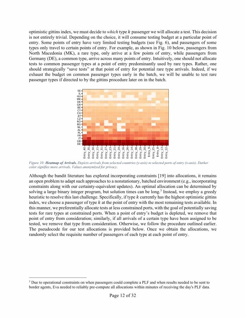
optimistic gittins index, we must decide to which type 𝑘 passenger we will allocate a test. This decision is not entirely trivial. Depending on the choice, it will consume testing budget at a particular point of entry. Some points of entry have very limited testing budgets (see Fig. 6), and passengers of some types only travel to certain points of entry. For example, as shown in Fig. 10 below, passengers from North Macedonia (MK), a rare type, only arrive at a few points of entry, while passengers from Germany (DE), a common type, arrive across many points of entry. Intuitively, one should not allocate tests to common passenger types at a point of entry predominantly used by rare types. Rather, one should strategically “save tests” at that point of entry for potential rare type arrivals. Indeed, if we exhaust the budget on common passenger types early in the batch, we will be unable to test rare passenger types if directed to by the gittins procedure later on in the batch.

Figure 10: Heatmap of Arrivals. Depicts arrivals from selected countries (y-axis) to selected ports of entry (x-axis). Darker color signifies more arrivals. Values anonymized for privacy.

Although the bandit literature has explored incorporating constraints [19] into allocations, it remains an open problem to adapt such approaches to a nonstationary, batched environment (e.g., incorporating constraints along with our certainty-equivalent updates). An optimal allocation can be determined by solving a large binary integer program, but solution times can be long.3 Instead, we employ a greedy heuristic to resolve this last challenge. Specifically, if type 𝑘 currently has the highest optimistic gittins index, we choose a passenger of type 𝑘 at the point of entry with the most remaining tests available. In this manner, we preferentially allocate tests at less constrained ports, with the goal of potentially saving tests for rare types at constrained ports. When a point of entry’s budget is depleted, we remove that point of entry from consideration; similarly, if all arrivals of a certain type have been assigned to be tested, we remove that type from consideration. Otherwise, we follow the procedure outlined earlier. The pseudocode for our test allocations is provided below. Once we obtain the allocations, we randomly select the requisite number of passengers of each type at each point of entry.

3 Due to operational constraints on when passengers could complete a PLF and when results needed to be sent to border agents, Eva needed to reliably pre-compute all allocations within minutes of receiving the day's PLF data.

of 32

Subroutine 3: Τest Allocation Sub-Routine

Input: Posterior distribution estimates 𝛼�2 , 𝛽�2 for each type 𝑘 ∈ 𝐾(, arrivals 𝐴2!(𝑡) and budgets 𝐵!(𝑡) for each type 𝑘 and point of entry 𝑒, number of pipeline tests 𝑄2 for each type 𝑘, and tuning parameters {𝑐, 𝛾}

for 𝑘 = 1:𝐾(

𝛼�2 ← c𝛼�2 , 𝛽�2 ← c𝛽�2# prior widening

Compute 𝜆2 from Eq. (6) using 𝛼�2 , 𝛽�2

𝜆2 ← pseudo-update index of type𝑘 (repeat 𝑄2 times) # account for pipeline tests

𝑌2 ← ∑ 𝐴2!(𝑡)! # type 𝑘 passengers not yet allocated a test

for 𝑒 = 1: ℰ

𝑌2! ← 𝐴2!(𝑡)# type 𝑘passengers at point of entry e not yet allocated a test

𝐶! ← 𝐵!(𝑡)# remaining (un-allocated) tests at point of entry e

𝑁2! ← 0 # initialize allocations

end

end

while maxF𝐶! > 0and max

>,!!∈{!|I'JK}𝑌2!! > 0

𝑘∗ = argmax2{𝜆2:𝑌2 > 0}

𝑒∗ = argmax!{𝐶!:𝑌2∗! > 0}

𝑁2∗!∗ ← 𝑁2∗!∗ + 1# allocate a test to a type k passenger at point of entry e

𝐶!∗ ← 𝐶!∗ − 1, 𝑌2∗!∗ ← 𝑌2∗!∗ − 1, 𝑌2∗ ← 𝑌2∗ − 1

𝜆2∗ ← pseudo-update index of type 𝑘∗

end

return {𝑁2!}2∈N),!∈{0,…,ℰ} # number of tests allocated to each type at each port of entry

Fig. 11 shows the resulting (anonymized) allocations for a typical day (batch) from the summer of 2020. The x-axis indexes different types ordered from highest prevalence (left) to lowest prevalence (right). Each bar denotes the number of arrivals. The teal portion represents the number of allocated tests, while the pink portion represents the remaining untested passengers. We observe that, as desired, our algorithm allocates tests to essentially all high-risk arrivals (exploitation) but additionally assigns a small number of tests to all types to reduce the variance of our estimates (exploration). The inclusion of port-specific constraints may cause some distortions, e.g., the lowest-risk type in Fig. 11 still

of 32

receives a large number of tests because these passengers arrived at a point of entry with atypically large testing capacity.

Figure 11: Test Allocations by Arrivals. Shows number of test allocations (teal) and untested scheduled arrivals (pink) for each type on a given day (batch). Types are ordered from high to low risk according to our empirical Bayes estimates of prevalence. Note that our algorithm allocates tests to essentially all high-risk arrivals (exploitation) but additionally assigns a small number of tests to all types (exploration).

2.3.6 Quantifying Exploration The gittins allocation scheme does not differentiate between tests allocated for exploration and exploitation. However, a reasonable proxy for the number of “exploration” tests may be the number of tests that were allocated on each day that a greedy policy would not allocate. Specifically, if 𝑛 tests are allocated on day 𝑡, we consider the fraction of tests that were allocated to passengers whose estimated prevalences were not among the top 𝑛 highest prevalences of arrivals that day. The left panel of Fig. 12 shows the results. We observe a noticeable spike in mid-August, corresponding to a change in Greek travel protocols where several countries were grey-listed on the same day; this induced a (temporary) surge in exploration to learn about the new grey-listed types. After this spike, the fraction of exploration tests stabilized to roughly 40% for the rest of the summer. A drawback of this proxy is that it does not distinguish between the “level of exploration” per test, i.e., did we allocate a test to a medium prevalence type (splitting the difference between exploration/exploitation) or to a low prevalence type (mostly exploration/no exploitation). In the previous metric, both instances are simply counted as 1 exploration test. Thus, we consider a second proxy for the amount of exploration: the average prevalence among passengers tested by Eva on day 𝑡 relative to the average (estimated) prevalence among passengers that would have been tested by a greedy exploitation-only strategy. If Eva were allocating all of its exploration tests to passengers with moderate/high prevalence, this difference will be small. If Eva were allocating all of its exploration tests to passengers with low prevalence, this difference will be large. The right panel of Fig. 12 shows the results. We see that, after the spike, exploration results in a roughly 20% reduction in average prevalence relative to a greedy strategy. This suggests that most exploration tests (identified in the previous metric) are actually partially exploiting by targeting types with medium prevalence.

of 32

Figure 12: Quantifying Exploration. Fraction of tests allocated for “exploration” (left) and the average prevalence of allocated tests relative to a greedy strategy (right) as a function of time. Plots depict 7-day rolling average. The spike in mid-August corresponds to a change in Greece’s travel protocols, inducing a temporary surge in exploration.

3 Off-Policy Evaluation and Counterfactual Analysis In this section, we detail our comparison of Eva’s historical performance to counterfactual estimates of the performance of other natural targeting policies: random surveillance testing and simple policies based on widely used epidemiological metrics. Specifically, in Sections 3.1, we benchmark against a random surveillance testing policy that tests passengers uniformly at random at each port of entry. In Section 3.2, we benchmark against policies which assign tests to travelers based on their country of origin and proportional to one of three country-level epidemiological metrics: cases per capita, deaths per capita, or positivity rates (number of positive cases found divided by number of tests performed in last 14 days). We calibrate each of these benchmark policies to have the same testing budget as Eva and to use the same grey-listing decisions. (See Section 5 below for more discussion of the effect of grey-listing decisions.) Before proceeding, we note that the historically realized data from Eva exhibits a significant no-show rate, i.e., passengers who filed a PLF but did not travel. Due to operational limitations, we do not know the actual number of type 𝑘 travelers who arrived at entry point 𝑒 on day 𝑡. Hence, we estimate this number as follows. Denote by 𝑇D2!(𝑡) the number of passengers of type 𝑘 that were actually tested at point of entry 𝑒 on day 𝑡 (as acknowledged by scanning their QR-code and associating it with a sample). Due to no-shows, this number may be less than 𝑇2!(𝑡), the number of passengers of type 𝑘 thatfiled a PLF and were allocated a test by Eva. We estimate the type- and entry-specific fraction of passengers that actually arrived by

𝑠2!(𝑡) =𝑇D2!(𝑡)𝑇2!(𝑡)

,

and estimate the actual arrivals by 𝐴�2!(𝑡) = 𝑠2!(𝑡)𝐴2!(𝑡). This estimate is unbiased because our decision to test a traveler is conditionally independent of their decision to not travel (“no-show”) given their type.

40%

60%

80%

100%

Sep Oct Nov

Expl

orat

ion

Test

s (%

of T

este

d)

20%

40%

60%

80%

Sep Oct Nov

Rel

ativ

e Pr

ev. o

f Exp

lora

tion

vs. G

reed

y

of 32

Finally, throughout this counterfactual analysis, we take types to be defined exclusively by the traveler’s country of origin (no adaptive type specification). This simplification permits a more straightforward computation of standard errors, and our estimators remain unbiased. 3.1 Defining the Benchmark Policies Let

• 𝑇D⋅!(𝑡) = ∑ 𝑇D2!(𝑡)2∈N) denote the total number of tests performed at entry 𝑒 • 𝑇D2⋅(𝑡) = ∑ 𝑇D2!(𝑡)ℰ

!/0 denote the total number of tests performed on type 𝑘 passengers • 𝐴�⋅!(𝑡) = ∑ 𝐴�2!(𝑡)2∈N) denote the (estimated) actual arrivals at entry 𝑒 • 𝐴�2⋅(𝑡) = ∑ 𝐴�2!(𝑡)ℰ

!/0 denote the (estimated) actual type 𝑘 arrivals across all entries. • 𝑥2(𝑡) denote one of cases per capita, deaths per capita, or positivity rate for country c where

type 𝑘’s country of origin is 𝑐

For any of our benchmark policies, let 𝜏2(𝑡) be the probability an arbitrarily chosen type 𝑘 arrival is tested at time t. For the random surveillance policy, by definition,

𝜏2Q65R(𝑡) = A𝐴�2!(𝑡)𝐴�2⋅(𝑡)

𝑇D⋅!(𝑡)𝐴�⋅!(𝑡)

ℰ

!/0

.

By contrast, our benchmark policy based on population-level epidemiological metrics tests a passenger with probability (roughly) proportional to their reported risk. Specifically, we first obtain the relevant pre-processed and smoothed time series 𝑥2(𝑡) for a given metric from https://ourworldindata.org/ [20, 21, 22]. We use the smoothed/pre-processed values instead of the the raw reported metrics since the raw data exhibit a number of missing or undefined (e.g., infinite) values and a number of “back-dated” corrections, i.e., negative counts to correct for over-reported metrics in previous days. Using this pre-processed data yields an optimistic analysis for the benchmark (pessimistic for Eva) since any real-time system based on epidemiological metrics would need to use the raw data as it was released in real-time, i.e., not adjusting for the back-dated corrections. (See Section 3.2.3 on “Drawbacks of Allocations Based on Epidemiological Metrics” for more discussion.) For allocations on day 𝑡, we use the value of the smoothed metric reported on day 𝑡 − 1 when available; when missing, we impute the value based on averaging the same metric across other countries on day 𝑡 − 1. Given this time series for 𝑥2(𝑡), our benchmark policy then tests a type 𝑘 arrival at time 𝑡 with probability proportional to 𝑥2(𝑡), i.e.,

𝜏2STU97A(𝑡) =A

𝐴�2!(𝑡)𝐴�2⋅(𝑡)

min ¦𝑥2(𝑡) ⋅ 𝑇D⋅!(𝑡)

∑ 𝐴�9!(𝑡)𝑥9(𝑡)9∈N), 1¨

ℇ

!/0

where the proportionality constant is chosen so that the expected number of tests at each point of entry is roughly equal to the number tested by Eva 𝑇D⋅!(𝑡). Inspired by soft-max heuristics in machine learning, we allocate tests proportionally to 𝑥2(𝑡) rather than entirely to countries with the maximum metric above. This choice is typically more effective with noisy data. For example, if there were only two countries, one with 100 deaths per capita and the other with 101 deaths per capita, it would be much more reasonable to assign tests roughly equally to both countries rather than all tests to the second country. Of course, when the gap in metrics is large, proportional allocation does allocate essentially all tests to the riskier country.

of 32

We say the expected number of tests at port 𝑒 allocated by this policy is tuned to “roughly” equal 𝑇D⋅!(𝑡) because we cap testing probabilities at 1 in the summand. (Probabilities above 1 are clearly infeasible.) This capping causes a small percentage of tests to be unused when rare arrivals at an entry point have particularly large values of 𝑥2(𝑡). To provide the fairest comparison, we correct for these unutilized tests below by comparing the number of cases caught per allocated test for these policies versus the cases caught per allocated test for Eva. In the special case that an epidemiological metric 𝑥2(𝑡) is identical for all (𝑘, 𝑡), the above policy reduces to the random policy. Note that the first branch of the “min” always pertains for the random policy, so it requires no correction for unutilized tests. 3.2 Background on Inverse Propensity Weight (IPW) Scoring While we directly observe Eva’s performance, we do not observe the performance of our benchmark policies, requiring us to estimate a counterfactual. We use a classical method, inverse propensity weight (IPW) scoring [23, 24], which is a model-agnostic approach. In particular, although our estimation and allocations entail several approximations, the IPW estimate of performance of the benchmark policies is conditionally unbiased (conditional on the arrival process of passengers) regardless of the quality of these approximations. Thus, this analysis provides a fair comparison between the Eva and any of the benchmarks. We perform all analysis conditional on the number and types of passengers that arrive at each time at each point of entry. We also note that only 0.6% of arrivals were tested by border agents at their own discretion (i.e., not recommended by Eva). Thus, unlike many IPW analyses, our test allocations do not suffer substantive unobserved confounding. For completeness, we drop these 0.6% of arrivals from the analysis. 3.2.1 Estimating Mean Performance We next summarize the pertinent details of the IPW method. Recall that 𝑃2!(𝑡) denotes the total number of positive type 𝑘 passengers identified by Eva at entry 𝑒, and that 𝑃2⋅(𝑡) is the number of positive type 𝑘 cases identified at time 𝑡 by Eva at all entries. The probability a type 𝑘 arrival would be tested at time 𝑡 by Eva is

A𝑇D2!(𝑡)𝐴�2!(𝑡)

ℰ

!/0

𝐴�2!(𝑡)𝐴�2⋅(𝑡)

= 𝑇D2⋅(𝑡)𝐴�2⋅(𝑡)

.

IPW scoring estimates the corresponding number for a benchmark policy by

𝑓2(𝑡) = 𝜏2(𝑡) ©𝑇D2⋅(𝑡)𝐴�2⋅(𝑡)

ª« × 𝑃2⋅(𝑡),

where the leading ratio is called the inverse propensity weight. In words, IPW scoring corrects the observed number of positives by multiplying by the relative likelihood of being tested under both methods. We then estimate the total number of positive cases that the benchmark would have caught by summing:

of 32

𝐼@!5AWX6Q2 =AA 𝑓2(𝑡)2∈N)

𝒯

(/0

It is common practice in the causal inference literature to drop elements of the summand for extreme values of the inverse propensity weight [23] to reduce variability. We follow this practice and drop any outlier (𝑒, 𝑡, 𝑘) combinations where the inverse propensity score exceeds the 97.5% quantile of all inverse propensity scores. To ensure fair comparison, we also drop the same elements from Eva’s performance when reporting relative improvements. Finally, for the policies based on epidemiological metrics, we additionally normalize the performance by the number of tests performed to ensure fair comparison. Specifically, we scale the number of estimated infections caught by the public policy by

𝜒STU97A = ¯AA𝑇!° (𝑡)ℰ

!/0

𝒯

(/0

± ²A A 𝜏2STU97A(𝑡)𝐴2⋅(𝑡)

2∈N)

𝒯

(/0

³ .´

Note that 𝜒STU97A ≥ 1 by construction; we estimate this scaling factor separately for peak and off-peak seasons for each epidemiological metric, with values ranging from 1.02 to 1.06. 3.2.2 Estimating the Variance We now turn to estimating the variance of 𝐼@!5AWX6Q2. Although 𝐼@!5AWX6Q2 is conditionally unbiased in a model-agnostic fashion, we require some modeling assumptions to approximate its variance. While recent work has developed methods to estimate this variance in classical bandit problems [25, 26], they require strong assumptions that do not hold in our setting, particularly that the underlying rewards are stationary and the amount of exploration is vanishing. Thus, we develop a new and conservative (worst-case) approximation for this variance in our highly non-stationary setting. Even if the assumptions underlying our approximation are mildly violated, our estimates are likely still valid because we adopt a worst-case perspective. To be precise, define 𝑌( =∑ 𝑓2(𝑡)2∈N) so that 𝐼@!5AWX6Q2 =∑ 𝑌(Y

(/0 . We upper bound the conditional variance of 𝐼@!5AWX6Q2 assuming that

I. No-show behavior at time 𝑡, i.e., the decision to not travel after filing a PLF, is independent across passengers.

II. The public epidemiological metric is such that there is no need to cap the probabilities at 1, i.e., the first branch of the “min” defining 𝜏2

STU97Aalways pertains. III. There exists a constant Δ such that for |𝑠 − 𝑡| ≥ Δ, the Correlation(𝑌( , 𝑌=) ≤ 0, i.e., the

autocorrelation of the process is negligible (or non-positive) after Δ days. We first argue that the three assumptions are reasonable. For the first, passenger cancellations on a given day 𝑡 are likely primarily driven by idiosyncratic/passenger-specific reasons (e.g., a relative is ill). Hence modeling them as independent across passengers is reasonable. For the second assumption, the probabilities exceed 1 relatively rarely (affecting only 2%-6% of allocated tests). Alternatively, we can interpret this assumption as saying that our analysis bounds the variance of a related random variable 𝐼ZQ["\, which is defined identically to 𝐼@!5AWX6Q2 but without the “min” in the definition of 𝜏2

STU97A. In so far as capping a random variable generally reduces its

of 32

variance, one intuitively expects the variance of 𝐼ZQ["\ bounds the variance of 𝐼@!5AWX6Q2, in line with our worst-case, conservative viewpoint. Finally, we recall that for the random policy, the capping is never needed, and, hence, this assumption is trivially satisfied. For the final assumption, observe that for Δ large enough, our estimates �̂�2?@(𝑡) and �̂�2?@(𝑠) are based on disjoint streams of testing data, because we discard old data. Moreover, even for small Δ, our prior-widening heuristic forces a certain minimal amount of exploration of each type (roughly 500 tests every 14 days), which occurs regardless of the results of previous tests. Thus, a large number of “exploration tests” are allocated independently of past test results and reduce dependence of future time periods on the past. In summary, there is good reason to believe our third assumption holds for some Δ,and we use our data to estimate a reasonable value. Fig. 13 plots an estimate of the autocorrelation of 𝑌( for our random surveillance policy at various lags after detrending the data and removing day of week effects with linear regression. For each lag 𝑙, the blue dotted lines represent an approximate two-sided 95% test statistic of the null hypothesis that the autocorrelation at lag 𝑙is zero, assuming the underlying process 𝑌( is stationary white noise. Similarly, for each lag, the red dotted lines represent an approximate two-sided 95% test statistic of the null hypothesis that the autocorrelation at lag 𝑙 is zero, assuming the underlying process 𝑌! is a moving average process of order 𝑙 − 1. (Computation of such confidence intervals is standard, e.g., see [27].) The plot suggests that the process does not exhibit autocorrelations that are statistically distinguishable from zero for lags greater than 7 days. Based on this analysis, we take Δ to be 8 days in what follows; our results are likely robust to small deviations of this value since we are performing a worst-case analysis.

Figure 13: Autocorrelation of Off-Policy Estimates. Autocorrelation of the (de-trended, de-seasonalized) time series 𝑌* defining the IPW estimate. Blue lines are a 95% test statistic (2-sided) for the null hypothesis that the autocorrelation is zero, assuming 𝑌* is white noise. Similarly, the red lines are a 95% test statistic (2-sided) for the null hypothesis that the autocorrelation at lag 𝑙is zero, assuming 𝑌* is a moving average process of order 𝑙 − 1. Results strongly suggest that autocorrelations die rapidly and are negligible after 1 week. Both test statistics computed using Bartlett’s Formula; see [27]. Time series of length T = 88 days used in estimation.

−0.5

0.0

0.5

1.0

0 5 10 15 20Lag (days)

Aut

ocor

rela

tion

of 32

We now derive a worst-case upper bound on the variance. We write our upper bound in the special case of our 𝑥2(𝑡) benchmark policy (recall that the estimate for the random surveillance policy is obtained by setting 𝑥2(𝑡)= 1 for all 𝑘, 𝑡.) We first group terms in the sum defining 𝐼@!5AWX6Q2 by days modulo Δ. Specifically, define

𝑍9 = A 𝑌((/9X[RT9[]

.

Then,

𝑉𝑎𝑟(𝐼@!5AWX6Q2) = 𝑉𝑎𝑟 ¯A𝑍9

]*0

9/K

± = AA 𝐶𝑜𝑣𝑎𝑟𝑖𝑎𝑛𝑐𝑒(𝑍9,𝑍X)]*0

X/K

]*0

9/K

≤ AA ¼𝑉𝑎𝑟𝑖𝑎𝑛𝑐𝑒(𝑍9)𝑉𝑎𝑟𝑖𝑎𝑛𝑐𝑒(𝑍X)]*0

X/K

]*0

9/K

where the last inequality follows by taking the worst-case assumption that each 𝑍9 has correlation one with each 𝑍X. In so far as each 𝑍9 is a sum of terms 𝑌( whose autocorrelation is approximated in Fig. 13 to be never more than 0.25, this upper bound is quite conservative. Under our assumption that autocorrelations of 𝑌( are negligible after Δ days, the terms of 𝑍9 are uncorrelated. Hence,

𝑉𝑎𝑟𝑖𝑎𝑛𝑐𝑒(𝑍9) = A 𝑉𝑎𝑟𝑖𝑎𝑛𝑐𝑒(𝑌().(/9X[RT9[]

By conditioning on information up to time 𝑡, the law of total variance shows (after some simplification)

𝑉𝑎𝑟𝑖𝑎𝑛𝑐𝑒(𝑌() = 𝑉𝑎𝑟𝑖𝑎𝑛𝑐𝑒 ²A 𝐴�2⋅(𝑡)𝑅2(𝑡)𝜏2(𝑡)2∈N)

³ + 𝐸 ¾A 𝑅2(𝑡)�1 − 𝑅2(𝑡)�2∈N)

𝐴�2⋅(𝑡)+𝜏2(𝑡)+

𝑇D2⋅(𝑡)¿.

A model-agnostic plug-in estimate of the second term above is

A �̂�25678!(𝑡) �1 − �̂�25678!(𝑡)�2∈N)

𝐴�2⋅(𝑡)+𝜏2(𝑡)+

𝑇D2⋅(𝑡).

Estimating the first term is more subtle. Using the expression for 𝜏2(𝑡) we can rewrite the relevant sum as

𝑉𝑎𝑟𝑖𝑎𝑛𝑐𝑒 ²A 𝐴�2⋅(𝑡)𝑅2(𝑡)𝜏2(𝑡)2∈N)

³ = 𝑉𝑎𝑟𝑖𝑎𝑛𝑐𝑒 ¯A𝑤!(𝑡)𝑇D⋅!(𝑡)ℰ

!/0

±,

where

𝑤!(𝑡) = ∑ 𝑅2(𝑡)𝑥2(𝑡)𝐴�2!(𝑡)2∈N)

∑ 𝑥2(𝑡)𝐴�2!(𝑡)2∈N).

The only source of randomness in the last expression is the random variables 𝑇D⋅!(𝑡). If the no-show rate were zero, 𝑇D⋅!(𝑡) would be deterministic because Eva always allocates the entire budget by

of 32

construction. The challenge is that when the no-show rate is non-zero, 𝑇D⋅!(𝑡) will be less than the testing budget at entry e. Fortunately, given our independence assumption on passenger no-show behavior,

𝑇D⋅!(𝑡) ∼ 𝐵𝑖𝑛𝑜𝑚𝑖𝑎𝑙(𝐵!(𝑡), 1 − 𝑞!5[*=W[^(𝑡)),

where we recall that 𝐵!(𝑡) is the testing budget at entry 𝑒 at time 𝑡, and 𝑞!5[*=W[^(𝑡) is the probability a passenger does not travel after filing a PLF. Moreover, 𝑇D⋅!(𝑡) is independent across 𝑒. Based on these observations, we let

𝑞�!5[*=W[^(𝑡) = 1 −𝑇D⋅!(𝑡)𝐵!(𝑡)

,

Then, by plugging in this estimate into the formula for the variance of a binomial distribution and leveraging the independence yields the plug-in estimate

𝑉𝑎𝑟𝑖𝑎𝑛𝑐𝑒 ¯A𝑤!(𝑡)𝑇D⋅!(𝑡)ℰ

!/0

± ≈ A𝑤!(𝑡)+𝑇D⋅!(𝑡)𝑞�!5[*=W[^(𝑡).ℰ

!/0

Combining all the pieces yields our final estimator of the variance.

𝑉𝑎𝑟(𝐼@!5AWX6Q2) ≲ ∑ ∑ ¼𝑣9 𝑣X]*0X/K

]*09/K ,

where

𝑣9 = A A �̂�25678!(𝑡) �1 − �̂�25678!(𝑡)�2∈N)

𝐴�2⋅(𝑡)+𝜏2(𝑡)+

𝑇D2⋅(𝑡)(/9X[RT9[]

+ A A𝑤!(𝑡)+𝑇D⋅!(𝑡)𝑞�!5[*=W[^(𝑡).ℰ

!/0(/9X[RT9[]

Note, in instances where we scale our estimate 𝐼@!5AWX6Q2 by 𝜒STU97A to account for unutilized tests, we scale the variance of our estimator by (𝜒STU97A)+. 3.2.3 Drawbacks of Allocating Tests Based on Epidemiological Metrics Beyond the quantitative assessment above, we highlight some qualitative drawbacks of policies based on epidemiological metrics:

1. Raw reported epidemiological data can be unreliable. In the months leading to Eva’s deployment (mid April to beginning of July, when the design was being crystallized), 51% of the daily tests performed and 12% of daily deaths were undefined (either due to periodic or inconsistent reporting) while 0.1% of reported deaths per capita were negative (see for example Fig. 14 below) among the countries from which we saw arrivals. This created serious concerns for the Eva team, epidemiologists and policymakers about making test allocations entirely based on these metrics. In our analysis, we use time series that were pre-processed by https://ourworldindata.org/ to correct for many of these issues with the benefit of hindsight, but

of 32

such corrections would not have been available in real-time. Finally, Greece has very little influence over real-time data quality as all data are provided (voluntarily) by other nations.

2. Using a policy based on epidemiological metrics requires a similar capital infrastructure investment as Eva, but obtains a fraction of the benefits. In particular, to implement the above policy, one would still need the PLF system to know the daily arrival mix across types in order to determine testing probabilities. Such infrastructure is not required for the random surveillance policy, where one can simply choose passengers out of the customs line without knowing anything about arrival rates, but this policy performs substantively worse.

3. These methods provide less effective surveillance. If a country's asymptomatic passenger

population had disproportionately high risk relative to its publicly reported epidemiological metrics, one would never know and might unintentionally admit many such passengers. This outcome is especially concerning since Eva's estimates were also used in other downstream policy decisions. For example, the ministry of Civil Protection combined Eva’s risk estimates with travelers’ within-country itineraries to identify areas within Greece that had a likely relatively high (incoming) viral load. For such areas, mobile testing teams were allocated in order to aggressively test the local and visiting population, and preemptively impose stricter social distancing rules if deemed necessary.

Figure 14: Reported daily deaths by Spain. Note the large negative value in late May that “corrected” previously reported cumulative counts. In addition, Spain abruptly stopped reporting daily deaths in late May and switched to cumulative reports.

4 Evaluating the Predictive Power of Epidemiological Metrics We now turn to evaluating more sophisticated functions of population-level epidemiological metrics on cases, deaths and testing rates [20, 21, 22] in predicting traveler prevalence at the Greek border. Recently, [28] used mathematical modeling to show that forecasting within epidemiological SIR models (through data-driven parametrization of model parameters) is not effective in predicting spikes in infections. Hence, in our analysis, we prefer the use of flexible, non-parametric methods like Gradient-Boosted regression Models (GBM) [29] for building predictive models.4 Specifically, GBM

4 Wherever we reference GBM, we have used the R implementation publicly available at: https://cran.r-project.org/web/packages/gbm/index.html tuned with 5 fold cross-validation.

−2000

−1000

0

1000

May Jun Jul

Dai

ly D

eath

s

of 32

is a machine-learning algorithm based on tree ensembles, which are known to perform well in structured classification tasks [30, 31]. 4.1 Predictive Value of Commonly Used Epidemiological Data We first provide details of our analysis of the predictive power of country level epidemiological data from the main text, namely, the ability of these data to predict whether a country was high-risk. We define a binary response variable for each country at each point in time as 1 if Eva’s estimated prevalence for that country was above 0.5%. We predict this binary response variable using gradient boosted regression models [29] with 500 trees and 5-fold cross-validation. These models have been shown to perform well across a variety of prediction tasks [30], but we also tested other predictive models such as LASSO and recurrent neural networks (RNNs) and obtained similar results. We use raw time series data for each epidemiological metric in this analysis, but we verified that we obtain essentially identical results with smoothed/pre-processed time series data. We evaluated different combination and granularities of public data, presented below:

• Model 1: Features are the 14-day average of cases and deaths per capita. • Model 2: Features are the 14-day average of cases, deaths and tests performed per capita, and

the positivity rate (number of positives divided by number of tests). • Model 3: Features are the 14-day timeseries of cases and deaths per capita. • Model 4: Features are the 14-day timeseries of cases, deaths and tests performed per capita,

and the positivity rate. • Model 5: Features are the 14-day timeseries of cases, deaths and tests performed per capita, the

positivity rate, and country fixed effects. For each model, we use the predictive performance on a held-out test set to assess the performance of our different estimators. Performance is measured by AUROC (area under ROC curve), which is a more informative metric than accuracy for imbalanced data [32]. Table 15 below reports the top features for each GBM model and their corresponding influence scores [29], which identify the features that most influence the resulting predictions. Feature Model 1 Model 2 Model 3 Model 4 Model 5 14-day avg of cases per capita 50% 29% - - - 14-day avg of deaths per capita 50% 30% 8% - - 14-day avg of tests per capita 25% - 5% 7% 14-day avg positivity rate 16% - - Cases per capita (today) 17% 11% 9% Cases per capita (1 day lag) 5% - - Deaths per capita (today) - 6% - Tests per capita (7 day lag) 12% 11% Tests per capita (12 day lag) 6% - Country fixed effect 25% AUROC 0.504 0.523 0.518 0.515 0.622

Table 15: GBM feature influence scores for each model. For clarity, we only report influence scores for features with at least 5% influence on the model’s prediction. A “–” denotes features that were included but had negligible feature influence. Therefore, columns may add to less than 100%.

of 32

Again, as discussed in the main document, all models except Model 5 offer minimal improvement over a model which predicts randomly. Importantly, country fixed effects have significant influence (25%) in Model 5. 4.2 Traveler Population vs. General Population As discussed in the main text, asymptomatic travelers to Greece from a particular country might exhibit fundamentally different demographic characteristics from that country’s general population. This difference would further explain why country-level epidemiological metrics are not very predictive of asymptomatic prevalence. To study this hypothesis, Fig. 16 below focuses on Germany, and compares the age distribution of the general adult population and travelers to Greece in summer of 2020. We focus on Germany as there were many German arrivals in our data, allowing for a large sample size. Perhaps expectedly, we observe that travelers are younger than the general population, suggesting a substantially different COVID-19 risk profile. There are likely many other distinguishing characteristics (e.g., socio-economic status, health risk), although these are difficult to quantify given the aggregated data Eva can access from the PLF. Nonetheless, these systematic differences underscore the need for reinforcement learning based methods that leverage testing data on the specific population of interest to make good testing decisions.

Figure 16: Population-Level vs. Traveler Age Distribution. Age distribution of adult German population (red) versus the adult travelers originating from Germany (teal). n =527,974 PLFs were used to estimate traveler age distribution.

4.3 Evaluation of Delay Between Prevalence and Public Case Data A second possible explanation for the poor predictive power of population-level epidemiological metrics are reporting delays. These delays might either be caused by information infrastructure (hospitals report up to a regional level on a weekly basis), or, more fundamentally, because COVID-19 patients typically exhibit a delay between infection and the onset of symptoms. Stressed healthcare systems in summer of 2020 may have focused testing on symptomatic populations, thus providing estimates that lag asymptomatic prevalence.

0.0%

4.0%

8.0%

12.0%

[15−20) [20−25) [25−30) [30−35) [35−40) [40−45) [45−50) [50−55) [55−60) [60−65) [65−70) [70−75) [75−80) [80−85) [85−90) [90−95) [95−100)Age Group (years)

Population

Travelers

of 32

To study potential delays, we focus on reported cases per capita. For each country, we aim to classify whether it is currently at risk, i.e., its prevalence (as measured by Eva) exceeds its median prevalence over the summer. Intuitively, if a country’s case data lags its underlying prevalence by ℓ days, then we can much more effectively predict its risk status 𝑦( on day 𝑡 using case data from ℓ days in the future, i.e., cases in the period [𝑡 + ℓ − 14, 𝑡 + ℓ]. Consequently, for each country, we build separate gradient boosted regression models for each ℓ ranging from 1 to 20. The left panel of Fig. 17 shows the resulting AUROC as a function of ℓ for 3 representative countries. A large AUROC for some ℓ suggests an information delay of ℓ days, e.g., France exhibits a delay of 8-9 days. We then use mixed-integer optimization to group countries into a small number of clusters with similar delays ℓ. In particular, we take as input the AUROC 𝐸Aℓ of the model for country 𝑐 with lag ℓ based on the above analysis. Then, for a given value of 𝑀 clusters, we solve the following binary optimization problem:

max`,\

AA𝐸Aℓ𝑧Aℓ

+K

ℓ/0

𝒞

A/0

𝑠. 𝑡. 𝑧Aℓ ∈ {0, 1}𝑧Aℓ ≤ 𝑦ℓfor all 𝑐 ∈ {1,… , 𝒞}

A 𝑧Aℓ = 1for all 𝑐 ∈ {1,… , 𝒞}+K

ℓ/0

A𝑦ℓ ≤ 𝑀+K

ℓ/0

Figure 17: Information Delays in Population-Level Cases. Left: AUROC for various ℓ for three representative countries: Austria (AT), France (FR), and Great Britain (GB). Large AUROC at lag ℓ suggests an information delay of ℓ days. The number of datapoints used to estimate the AUROC at each lag l above ranges from 70 to 90 (depending on the lag used). Right: Elbow graph of the objective value of the optimization problem vs the number of clusters M. The sharp change in slope at 3 suggests three clusters in the data.

This optimization assigns each country to a single lag, encoded by the decision variable 𝑧Aℓ. Every country must be assigned some lag (the first equality constraint). The first inequality constraint ensures that the variables 𝑦ℓ will be equal to 1 and non-zero only if some country was assigned lag ℓ. The final

0.5

0.6

0.7

0.8

0.9

0 5 10 15Lag (days)

AU

ROC

AT

FR

GB

0.700

0.725

0.750

2 4 6 8 10Number of Clusters

Avg.

AU

C

of 32

inequality constraint ensures that there are no more than 𝑀 distinct lags to which countries are assigned. In other words, the optimization seeks a clustering of countries to lag with minimal error and no more than 𝑀 clusters. We solved this optimization for various values of 𝑀 and used the common heuristic of looking for an “elbow” in the resulting objective (see right panel of Fig. 17) to select 𝑀 = 3. Fig. 18 identifies the resulting three clusters of delays: short (1 day), medium (9 days) and long (16 days), as well as representative countries in each cluster.

Figure 18: Information Delays across Countries. Three clusters are identified with Short (1 day), Medium (9 days) and Long (16 days) information delays. The table lists representative countries from each cluster.

5 Grey-listing Counterfactuals Although not a fully algorithmic element of Eva’s deployment, grey-listing decisions were partially made on the estimates produced by Eva. We next examine some aspects and consequences of the grey-listing decisions in summer 2020. For completeness, the complete list of countries that were grey-listed and the time at which they were grey-listed is in Table 19.

ISO Code Start Date End Date BG 2020-07-28 - RO 2020-07-28 - MT 2020-08-12 - SE 2020-08-18 - BE 2020-08-18 - ES 2020-08-18 - NL 2020-08-01 2020-08-31 IL 2020-09-14 - CZ 2020-09-28 - PL 2020-10-03 -

Table 19: Grey-listed Countries. Over summer 2020, 10 countries were grey-listed. These are listed above with day that grey-listing began, and, in the case of the Netherlands, the day grey-listing ended. All other countries remained grey-listed for the duration of Eva’s operation.

10

11

4

0

3

6

9

12

Short Medium Long

Delay (days) Countries (ISO Code)

Short (1) PL, EG, RU, HR, MK, CI, LU, SK, IE, GB

Medium (9) PH, CN, US, PK, AL, DK, FR, IL, CY, TR, BA

Long (16) CH, AT, NO, RS

of 32

Grey-listing has two effects: it reduces the prevalence of infections among arrivals (because all arrivals are required to obtain a negative PCR test) and it reduces arrivals (because it is difficult or inconvenient for tourists to obtain a test). To assess the impact of our grey-listing policy, we must estimate the counterfactual prevalence and arrival rate that would have occurred had we not grey-listed a nation. For both estimates, we use gradient boosted regression models (GBM). Specifically, our models are as follows: Counterfactual Prevalence Model: The unit of observation is a country-date pair and the response is the prevalence estimated by Eva. We have training data from white-listed and grey-listed countries prior to grey-listing, as well as training data from white-listed countries post grey-listing. Our features included time series data of publicly reported cases, deaths and testing rates for each day within a [−20,+20] day range, a categorical country variable to control for fixed-effects, as well as the date (to capture global time trends). Note that we include data from future dates to account for the information lag in public data. The resulting prevalence model was used to predict the prevalence for grey-listed countries prior to grey-listing (in-sample) and up to 9 days post grey-listing (out-of-sample); the latter yields counterfactual prevalence estimates to infer the number of infections prevented by grey-listing. The left panel of Fig. 20 depicts the results for Malta; as desired, we observe a close match between the true and counterfactual prevalence prior to grey-listing. Observe that our prevalence estimates indicate a sustained drop in prevalence among arrivals from the grey-listed country. One week after grey-listing, we still see a 44% reduction on average in prevalence for grey-listed countries relative to the non-grey-listed counter factual estimates. Counterfactual Arrivals Model: The unit of observation is every grey-listed country-date pair and the response is the 7-day rolling average number of arrivals from that country on that day. We have training data from all countries prior to grey-listing, as well as training data from non-grey-listed countries post grey-listing. Our features included current total arrivals from white-listed countries, total arrivals from black-listed countries, a categorical country variable, as well as the date (to capture global time trends). One concern is that, as discussed earlier, a significant fraction of scheduled arrivals does not materialize at the border, and this varies by country. However, our data suggests that the no-show rate does not materially change due to the grey-listing policy. Thus, we compute a single no-show rate per country, and use this as a multiplier on both actual and predicted arrival rates to calculate actual arrivals. The resulting arrivals model was used to predict arrivals for grey-listed countries prior to grey-listing (in-sample) and up to 9 days post grey-listing (out-of-sample); the latter yields counterfactual arrival estimates to infer the number of infections prevented by grey-listing. The right panel of Fig. 20 depicts the results for Malta; as desired, we observe a close match between the true and counterfactual arrivals prior to grey-listing. These predictions also indicate a sustained drop in arrivals from the grey-listed country. In particular, one week after grey-listing, we see a 39% reduction on average in arrivals for grey-listed countries relative to the non-grey-listed counter factual estimates.

of 32

Figure 20: Grey-listing Counterfactuals for Malta. Measured and counterfactually estimated prevalence (left) and arrival rates (right) for Malta before and after-grey-listing. Grey-listing occurred on 12 Aug (dotted line). As desired, the models visually track both true prevalence and true arrival rates well prior to the grey-listing intervention (overlapping lines). The counterfactuals in the left and right panels were estimated on n=14,748 and n=460 observations respectively.

5.1 From Counterfactual Analysis to the Value of Grey-listing One might argue that our analysis in Section 3 of the performance of benchmark policies is overly optimistic for the benchmarks (pessimistic for Eva), because we assumed these benchmarks implemented the same grey-listing decisions as Eva. Absent Eva’s reinforcement learning, grey-listing decisions would necessarily be made on publicly available epidemiological data, and, in light of our results in Section 4 on the limited predictive power of country-level epidemiological data, it is not obvious such decisions would perform as well. Hence, we next attempt to quantify the benefit Eva enjoyed due to its grey-listing decisions relative to a policy that would grey-list the same countries as Eva, but 9 days later (based on our lag analysis in Section 4).

In more detail, grey-listing functionally causes infected passengers to stay in their origin country and not travel to Greece, either because they cannot easily obtain an PCR test, or their PCR test indicates they are infected. We use the above counterfactual analysis to estimate the number of infections that Eva prevented by grey-listing as

𝐴�2bIc(𝑡)�̂�2bIc(𝑡) −𝐴�2(𝑡)�̂�2?@(𝑡),

where�̂�2bIc(𝑡), 𝐴�2bIc(𝑡) are the model predictions for prevalence and arrivals under the grey-listing counterfactual from the previous subsection. The above difference is then an estimate of the total number of infected arrivals in the non-grey-listed scenario minus the total number of infected arrivals in the grey-listed scenario. Notice all these infections were prevented by Eva since none of them arrived in Greece (they remained home and did not travel). We sum this contribution up for every day in the 9 days following grey-listing for every country that was grey-listed to form our estimate of the value of grey-listing in the main paper.

Aug Sep Oct Nov

Prev

alen

ce (A

nony

miz

ed)

Actual

Counterfactual

Aug Sep Oct Nov

Arri

vals

(PLF

s)

Actual

Counterfactual

of 32

5.1.1 Estimating the Variance We estimate the variance of this value of grey-listing conditional on the arrival process. The dominant term in the variance stems from the variability of 𝐴�2bIc(𝑡)�̂�2bIc(𝑡), and, in particular, from variability in our grey-list counterfactual estimation procedure above. Hence, we focus on quantifying this variability. Specifically, for each counterfactual model, we evaluate the prediction error by splitting our original training dataset into a training set (70% of observations) and test set (30% of observations). The residuals on the test set 𝑦 − 𝑦� appear roughly normally distributed in both cases. Denote the variance of the residuals as 𝜎SQ!8+ for predicting prevalence, and 𝜎6QQ+ (𝑐) for predicting arrivals for country 𝑐.5 Thus, we model our counterfactual estimates of prevalence and arrivals as normal random variables, centered around the predicted value with variance given by 𝜎SQ!8+ and 𝜎6QQ+ (𝑐) respectively. We then compute the value of grey-listing 9 days later than Eva (as described above) across 1 million Monte Carlo simulations to numerically estimate its variance. 5.1.2 Results For privacy reasons, we again present results scaled by an arbitrary constant which is taken to be the actual number of infections identified by Eva in summer 2020 for ease of comparison. During the peak season, Eva prevented an additional 6.7% (±1.2%) asymptomatic, infected travelers from entering through its early grey-listing decisions. In the off-peak season, this number was similar 6.8% (±0.5%). In both cases, for privacy reasons we have expressed the benefit (and standard error) relative to the actual number of infected travelers identified by Eva in the corresponding period.

6 Data Governance, Storage, Privacy The Greek Government detailed its travel protocols and intent to carry out diagnostic screening throughout the 2020 Tourist season in Joint Ministerial Decision Nr. Δ1αΓΠ. oικ 40383/28.6.2020 (Journal of Greek Government, B’ 2602). This document outlines both the collection and storage of PLF data and testing results. Here, we only summarize pertinent details. A complete Privacy Policy issued by the Greek Government is available at [4], including details on travelers’ rights to amending or requesting deletion of their data, routine personal data deletion procedures, and other legal details. In GDPR terminology, the General Secretariat of Civil Protection (GSCP) in the Greek Government is the “Controller” of the personal data. Similarly, the Ministry of Digital Governance (MDG) is the “Processor” of the data. Both the GSCP and MDG committed to a high level of protection of travelers’ personal data in accordance with all EU regulations, GDPR, and Greek law. GSCP collected travelers’ personal data (with consent) via the Passenger Locator Form (PLF). These personal data were necessary for contact tracing and other public safety measures. This collection and processing of data is necessary (Art 6 GDPR) for the performance of a task carried out in the public interest (for the protection of Public

5 We used a single model to predict prevalence for all countries, but we used a separate country-specific model to predict arrivals for each grey-listed country. These decisions were made to improve out-of-sample accuracy.

of 32

Health) and in the exercise of official authority vested in the controller (9 ar. 9 par. 2 i, Greek Law 4624/2019 ar. 22 par. 1 c). Data were stored on a cloud-server located in European Union and encrypted using the (industry standard) AES-256 encryption algorithm. The source code that implements the algorithms described in the paper resided on the servers of the Controller, received pseudonymized/aggregated data from the Controller and output data (testing recommendations) to the Controller. Researchers only have access to the source code that implements the algorithm for maintenance purposes but do not have access rights to read or write data from or to the database clusters of the Controller. At no point did researchers have access to personal data since the processing, reading and writing from the database clusters of the Controller can only be performed by the Processor and the Controller (who ensure GDPR compliance as described above).

7 Other Technical Implementation Details Eva can roughly be described as four modules:

1. The Application Communication Interface (API) used for communication with the Greek data provider (GR-DB)

2. The Eva Engine 3. The Continuous Deployment System

These modules were contained in the same Virtual Private Cloud (VPC) and, to ensure privacy, no incoming communication to the open internet was allowed. Any incoming or outgoing data connections with GR-DB took place through a common VPC using the API module. The API module operated on AWS Lambda, the serverless computing service of Amazon. The API had two serverless functions: one responsible for data ingestion, and the other for communication of results back to GR-DB. To provide additional security, token-based authentication was implemented and enforced, and all authentication attempts were logged. The Eva Engine module operated on Amazon Elastic Compute Cloud (EC2) on an 8 V-CPU and 32 GiB Memory server. It contained the code for running the Eva algorithm, which outputs daily test allocations given recent testing results and the current passenger manifest. The results were stored for analysis purposes to the Database and were also transformed to various formats to be sent to the API. A Continuous Deployment system was in place to ensure that updates to the code could be deployed easily and safely in the API or the Eva engine, while offering functionality for logging, notifications and rollback. There were three identical versions of the Eva system all running in parallel: a production version that had the latest verified and approved code, a “staging” version that had code that had not yet been verified for validity, and a development version for active research and development. The daily cost of the Eva portion of the system ranged from $17 to $25 per day.

of 32

8 Bibliography [1] T. L. Lai and H. Robbins, "Asymptotically efficient adaptive allocation rules," Advances in applied

mathematics, pp. 4-22, 1985. [2] W. Thompson, "On the likelihood that one unknown probability exceeds another in view of the

evidence of two samples," Biometrika, pp. 285-294, 1933. [3] J. Gittins, "Bandit processes and dynamic allocation indices," Journal of the Royal Statistical

Society: Series B (Methodological), pp. 148-164, 1979. [4] Ministry of Civil Protection and Ministry of Tourism, Hellenic Republic, "Protocol for Arrivalsin

Greece," 2020. [Online]. Available: https://travel.gov.gr/#/policy. [5] H. Luo, C.-Y. Wei, A. Agarwal and J. Langford, "Efficient contextual bandits in non-stationary

worlds," Conference on Learning Theory, pp. 1739-1776, 2018. [6] P. Zhao, L. Zhang, Y. Jiang and Z.-H. Zhou, "A simple approach for non-stationary linear bandits,"

International Conference on Artificial Intelligence and Statistics, pp. 746-755, 2020. [7] O. Besbes, Y. Gur and A. Zeevi, "Stochastic multi-armed-bandit problem with non-stationary

rewards," Advances in neural information processing systems, pp. 199-207, 2014. [8] A. B. Tsybakov, Introduction to Nonparametric Estimation, Springer, 2009. [9] S. Greenland and J. Robins, "Empirical-Bayes adjustments for multiple comparisons are sometimes

useful," Epidemiology, pp. 244-251, 1991. [10] O. J. Devine, T. Louis and E. Halloran, "Empirical Bayes methods for stabilizing incidence rates

before mapping," Epidemiology, pp. 622-630, 1994. [11] R. Tibshirani, "Regression shrinkage and selection via the lasso," Journal of the Royal Statistical

Society: Series B (Methodological), pp. 267-288, 1996. [12] H. Bastani and M. Bayati, "Online decision making with high-dimensional covariates," Operations

Research, pp. 276-294, 2020. [13] P. Auer, "Using confidence bounds for exploitation-exploration trade-offs," Journal of Machine

Learning Research, pp. 397-422, 2002. [14] E. Gutin and V. Farias, "Optimistic gittins indices," Advances in Neural Information Processing

Systems, pp. 3153-3161, 2016. [15] V. Perchet, P. Rigollet, S. Chassang and E. Snowberg, "Batched bandit problems," The Annals of

Statistics, pp. 660-681, 2016. [16] Z. Gao, Y. Han, Z. Ren and Z. Zhou, "Batched multi-armed bandits problem," Advances in Neural

Information Processing Systems, pp. 503-514, 2019. [17] H. Bastani, D. Simchi-Levi and R. Zhu, "Meta Dynamic Pricing: Transfer Learning Across

Experiments," Management Science (forthcoming), 2021. [18] S. Agrawal and N. Goyal, "Thompson sampling for contextual bandits with linear payoffs,"

International Conference on Machine Learning, pp. 127-135, 2013. [19] S. Agrawal and N. Devanur, "Bandits with concave rewards and convex knapsacks," Proceedings of

the fifteenth ACM conference on Economics and computation, pp. 989-1006, 2014. [20] J. Hasell, E. Mathieu, D. Beltekian, B. a. G. C. a. O.-O. E. Macdonald, M. Roser and H. Ritchie, "A

cross-country database of COVID-19 testing," Scientific data, vol. 7, no. 1, pp. 1-7, 2020. [21] M. Roser, H. Ritchie, E. Ortiz-Ospina and J. Hasell, "Coronavirus Pandemic (COVID-19),"

OurWorldInData.org, 2020. [Online]. Available: https://ourworldindata.org/coronavirus. [22] E. Dong, H. Du and L. Gardner, "An interactive web-based dashboard to track COVID-19 in real

time," The Lancet infectious diseases, vol. 20, no. 5, pp. 533-534, 2020.

of 32

[23] W. G. Imbens and B. D. Rubin, Causal Inference in Statistics, Social and Biomedical Sciences, Cambridge University Press, 2015.

[24] P. Rosenbaum and D. Rubin, "The central role of the propensity score in observational studies for causal effects," Biometrika, vol. 70, no. 1, pp. 41-55, 1983.

[25] X. Nie, X. Tian, J. Taylor and J. Zou, "Why adaptively collected data have negative bias and how to correct for it," in International Conference on Artificial Intelligence and Statistics, 2018.

[26] V. Hadad, D. A. Hirshberg, R. Zhan, S. Wager and S. Athey, "Confidence intervals for policy evaluation in adaptive experiments," arXiv, 2019.

[27] P. Brockwell and R. Davis, Introduction to Time Series Forecasting, Springer, 2016. [28] J. Baek, V. Farias, A. Georgescu, R. Levi, T. Peng, D. Sinha, J. Wilde and A. Zheng, "The limits to

learning an SIR process: granular forecasting for COVID-19," arXiv, 2020. [29] Friedman, "Greedy function approximation: a gradient boosting machine," Annals of statistics, pp.

1189-1232, 2001. [30] A. Fogg, "Anthony Goldbloom gives you the secret to winning Kaggle competitions," 13 January

2016. [Online]. Available: https://www.import.io/post/how-to-win-a-kaggle-competition/. [31] "What algorithms are most successful on Kaggle?," [Online]. Available:

https://www.kaggle.com/bigfatdata/what-algorithms-are-most-successful-on-kaggle. [32] J. Friedman, T. Hastie and R. Tibshirani, The elements of statistical learning, New York: Springer

Series in Statistics, 2001.

Efficient and Targeted COVID-19 Border Testing via ...

Documents

Transcript of Efficient and Targeted COVID-19 Border Testing via ...