arX

iv:1

006.

0151

v1 [

cond

-mat

.sta

t-m

ech]

1 J

un 2

010

EFFECTS OF QUENCHED RANDOMNESS ON

CLASSICAL AND QUANTUM PHASE TRANSITIONS

BY RAFAEL L. GREENBLATT

A dissertation submitted to the

Graduate School—New Brunswick

Rutgers, The State University of New Jersey

in partial fulfillment of the requirements

for the degree of

Doctor of Philosophy

Graduate Program in Physics and Astronomy

Written under the direction of

Joel L. Lebowitz

and approved by

New Brunswick, New Jersey

October, 2010

ABSTRACT OF THE DISSERTATION

Effects of Quenched Randomness on Classical and

Quantum Phase Transitions

by Rafael L. Greenblatt

Dissertation Director: Joel L. Lebowitz

This dissertation describes the effect of quenched randomness on first order phase tran-

sitions in lattice systems, classical and quantum. It is proven that a large class of

quantum lattice systems in low dimension (d ≤ 2 or, with suitable continuous sym-

metry, d ≤ 4) cannot exhibit first-order phase transitions in the presence of suitable

(“direct”) quenched disorder.

ii

Acknowledgements

Nothing is ever truly the work of a single person. Much of the content of this disserta-

tion was shaped in the course of conversations with colleagues and many distinguished

scientists, among them Royce Zia, Moshe Schechter, Enza Orlandi, Vieri Mastropi-

etro, Tobias Kuna, Michael Kiessling, Sheldon Goldstein, Alessandro Giuliani, Gio-

vanni Gallavotti, Diana David-Rus, Eric Carlen, Gabe Bouch, and especially Michael

Aizenman.

Anything else achieved here would have been impossible without the support and

encouragement of my friends; besides those I have already listed above, I owe special

thanks to Joe Cleffie, Anand Gopal, Alicia Graham, Sarah Grey, and Pankaj Mehta. I

am also grateful to my brothers and sisters in the Rutgers Council of AAUP Chapters-

AFT for all they have done to improve the working lives of graduate employees like

myself.

Ron Ransome, the director of the physics graduate program for most of my time

here, has been extremely helpful at many points, particularly in making it possible for

me to resume my studies after an interruption.

Above all, I thank my advisor and mentor, Joel Lebowitz, who has helped me (like so

many other students) in more ways than I can express here, not least by the remarkable

example he has set for all of us.

iii

Dedication

To my first math teacher and my first physics teacher:

my mother, Susan Selvig

and my father, Richard Greenblatt

iv

Table of Contents

Abstract . . . . . . . . . . . . . . . . . . . . . . . . . . . . . . . . . . . . . . . . ii

Acknowledgements . . . . . . . . . . . . . . . . . . . . . . . . . . . . . . . . . iii

Dedication . . . . . . . . . . . . . . . . . . . . . . . . . . . . . . . . . . . . . . . iv

List of Figures . . . . . . . . . . . . . . . . . . . . . . . . . . . . . . . . . . . . viii

1. Introduction . . . . . . . . . . . . . . . . . . . . . . . . . . . . . . . . . . . 1

1.1. The rounding effect for classical systems . . . . . . . . . . . . . . . . . . 2

1.1.1. Ising models . . . . . . . . . . . . . . . . . . . . . . . . . . . . . 5

Nearest neighbor Ising chain at zero temperature . . . . . . . . . 6

Long range interactions in one dimension . . . . . . . . . . . . . 8

Higher dimensions . . . . . . . . . . . . . . . . . . . . . . . . . . 9

1.1.2. The 3 dimensional XY model . . . . . . . . . . . . . . . . . . . . 10

1.2. The rounding effect for quantum systems . . . . . . . . . . . . . . . . . 12

1.2.1. Transverse field Ising models: direct and orthogonal randomness 12

1.2.2. The quantum Ashkin-Teller chain: an exception? . . . . . . . . . 13

2. Proof of the rounding effect: overview and preliminaries . . . . . . . 15

2.1. Notation and systems under consideration . . . . . . . . . . . . . . . . . 16

2.1.1. Systems with continuous symmetries . . . . . . . . . . . . . . . . 22

2.2. Thermodynamic limit and notions of long range order . . . . . . . . . . 24

2.3. Statement of main results . . . . . . . . . . . . . . . . . . . . . . . . . . 26

3. A nonlinear central limit theorem . . . . . . . . . . . . . . . . . . . . . . 28

3.1. Background . . . . . . . . . . . . . . . . . . . . . . . . . . . . . . . . . . 28

3.2. Definitions . . . . . . . . . . . . . . . . . . . . . . . . . . . . . . . . . . . 29

v

3.3. The proposition . . . . . . . . . . . . . . . . . . . . . . . . . . . . . . . . 30

3.4. Proof of Proposition 3.3.1 . . . . . . . . . . . . . . . . . . . . . . . . . . 33

3.5. Bounds on b2 . . . . . . . . . . . . . . . . . . . . . . . . . . . . . . . . . 37

4. Free energy fluctuations . . . . . . . . . . . . . . . . . . . . . . . . . . . . 39

4.1. Definition of GL . . . . . . . . . . . . . . . . . . . . . . . . . . . . . . . 39

4.2. Proof of proposition 4.1.1 - finite temperature . . . . . . . . . . . . . . . 41

4.3. Proof of proposition 4.1.1 for absolutely continuous distributions of η . . 44

4.4. Proof of Proposition 2.3.1 . . . . . . . . . . . . . . . . . . . . . . . . . . 46

4.5. Systems with continuous symmetry: Proof of Proposition 2.3.2 . . . . . 48

5. Conclusion . . . . . . . . . . . . . . . . . . . . . . . . . . . . . . . . . . . . 53

Appendix A. Methods for numerical studies of random field spin systems 54

A.1. The maximum flow representation of the Ising model ground state . . . 54

A.2. Monte Carlo methods for XY and clock models . . . . . . . . . . . . . . 56

A.2.1. The lookup table algorithm for the Clock model . . . . . . . . . 56

A.2.2. A modified Ziggurat algorithm for the XY model . . . . . . . . . 58

Appendix B. Rounding of First Order Transitions in Low-Dimensional

Quantum Systems with Quenched Disorder . . . . . . . . . . . . . . . . . 61

Appendix C. Some concepts and results in mathematical probability . 70

C.1. σ-algebras and measures . . . . . . . . . . . . . . . . . . . . . . . . . . . 70

C.2. Lp norms and spaces; convergence of measurable functions . . . . . . . . 72

C.3. Random variables, expectations, conditional expectations . . . . . . . . 74

Appendix D. Product Measure Steady States of Generalized Zero Range

Processes . . . . . . . . . . . . . . . . . . . . . . . . . . . . . . . . . . . . . . . 76

D.1. Introduction . . . . . . . . . . . . . . . . . . . . . . . . . . . . . . . . . . 76

D.2. Factorizability in the Mass Transport Process . . . . . . . . . . . . . . . 80

D.3. Reverse processes . . . . . . . . . . . . . . . . . . . . . . . . . . . . . . . 83

vi

D.4. Factorizability in Generalized Zero Range Processes . . . . . . . . . . . 84

D.5. GZRPs on infinite lattices . . . . . . . . . . . . . . . . . . . . . . . . . . 85

D.6. Conclusion . . . . . . . . . . . . . . . . . . . . . . . . . . . . . . . . . . 86

References . . . . . . . . . . . . . . . . . . . . . . . . . . . . . . . . . . . . . . . 88

Vita . . . . . . . . . . . . . . . . . . . . . . . . . . . . . . . . . . . . . . . . . . . 92

vii

List of Figures

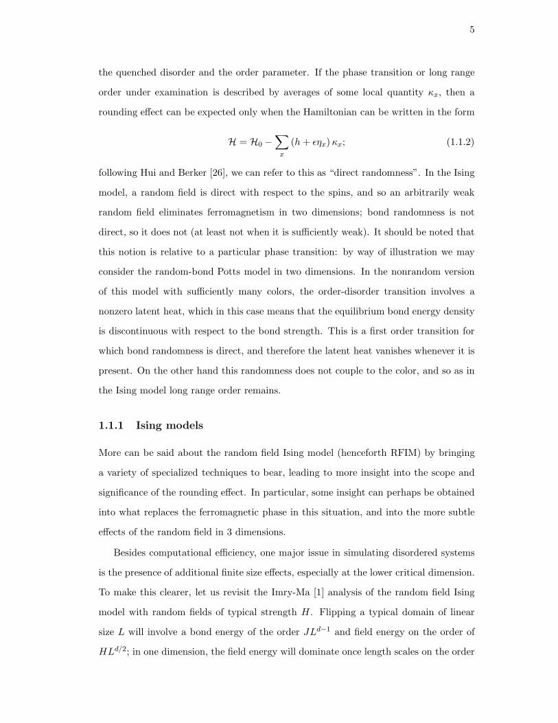
1.1. Plot of ground state magnetization as a function of mean magnetic field

h0 for a random field Ising chain with magnetic field distribution 12δh−H+

12δh+H , J = 1, H = 0.42 . . . . . . . . . . . . . . . . . . . . . . . . . . . 8

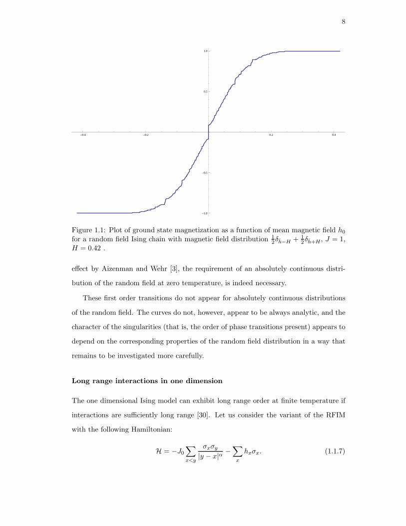
1.2. A two-dimensional example of a dichotomous random field configuration

leading to “Perestroika” in the ground state. The bold lines divide sepa-

rate regions where the spins are always +, indeterminate, and always −

in any ground states. . . . . . . . . . . . . . . . . . . . . . . . . . . . . 9

A.1. Example of the maximum flow graph used to derive Equation (1.1.5) . 56

A.2. The ziggurat algorithm: a probability density, bounding boxes of equal

volume . . . . . . . . . . . . . . . . . . . . . . . . . . . . . . . . . . . . . 59

A.3. The modified ziggurat algorithm: two probability densities, bounding

boxes of equal volume. The probability densities shown are those of

Equation (A.2.3), with k = 1 and k = 1.5, rescaled for pk(0) = 1. . . . . 60

viii

1

Chapter 1

Introduction

One of the basic techniques of condensed matter physics is the effective description

of solids as a combination of a static portion and a rapidly-moving part: in a simple

description of metals, the nuclei and tightly-bound electrons remain fixed and form an

effective potential background for the conduction electrons. Although the simplest de-

scription involves a uniform or periodic background (i.e. a perfect crystal), this is hardly

a natural assumption: completely pure samples are anything but common or easily pre-

pared. There are many situations in which disorder has only a minor effect, but there

are cases of fundamental importance where this is not the case. The best-established

illustration is the description of electrical conduction in metals: with the application

of quantum mechanics in this context it became clear that irregularly-placed scatter-

ers were necessary to account for finite conductivity. Anderson localization provides

a further way in which disorder produces a qualitative difference in the behavior of a

physical system.

These examples concern transport properties, which are harder to fit into a compre-

hensive framework than equilibrium properties. The core of the work described here is

a similarly qualitative effect at the level of equilibrium thermodynamics, the rounding

effect predicted by Imry and Ma [1] and described in detail in the next section.

It is misleading in a way to talk about equilibrium in this context. As noted already

in the paper which introduced the mathematical framework now known as quenched

randomness [2], it is important to consider a background which is a metastable configu-

ration, and is not typical of the equilibrium state of the full system. Although disorder

is still present in systems which are genuinely in equilibrium (this is what is known as

annealed disorder), annealed systems cannot exhibit behavior which is fundamentally

2

different from that of ordered systems.

There is still much that remains to be understood about classical models of quenched

randomness, but the situation for quantum systems has been even more obscure. The

main results presented in this dissertation, Propositions 2.3.1 and 2.3.2, are an extension

of the proof of the Imry-Ma rounding effect to quantum systems. The present chapter

will discuss the previous state of understanding and attempt to provide context for the

result. Chapters 2 to 4 comprise the proof of these results. Chapter 2 describes the

formalism used, establishes several preliminary results, and states the main proposi-

tions to be established. Chapter 3 contains a proof of a nonlinear central limit theorem

(based on an earlier result of Aizenman and Wehr [3]) which may be of some inde-

pendent interest. Chapter 4 completes the proof of the main results with an analysis

of the free energy effects of the quenched randomness. This work was announced in

a publication by the author with M. Aizenman and J. L. Lebowitz, which provides a

summary of the argument as is therefore attached as [4]. Additionally, Appendix C

reviews some probabilistic terminology and results used in the previous chapters which

may be unfamiliar to some readers.

Appendix D (written with J.L. Lebowitz, and published as [5]) describes earlier

work by the author, with J. L. Lebowitz, on nonequilibrium stochastic dynamics.

1.1 The rounding effect for classical systems

A 1975 paper by Imry and Ma contains an important insight into phase transitions

in disordered systems based on an analysis of the energy of the ordered phase, using

considerations similar to those applied more rigorously in Peierls’ proof of long range

order in the Ising model [6] and later in Pfister’s proof of the Mermin-Wagner theorem

for classical systems [7]. The context is O(N) models, that is lattice models where

configurations consist of a specification of an N -dimensional unit vector (a classical

spin) ~σx at each site x, with equilibrium states determined by the Hamiltonian

H = −J∑

~σx · ~σy −∑

~hx · ~σx. (1.1.1)

Since the paramagnetic phase of this system has higher entropy, for the ordered

3

phase to be stable requires that the energy cost involved in forming a domain where

the spins inside are aligned in a different direction from those outside grow with the

size of such a domain. In the Ising (N = 1) case the cost for a domain of diameter L is

of order Ld−1, and in continuous (N ≥ 2) versions spin-wave analysis [8] suggests a cost

on the order of Ld−2. In the absence of a random field this suggests (correctly) that

ferromagnetism does not exist in these systems at finite temperature for d = 1 and d ≤ 2

respectively. Since ferromagnetism appears at any higher dimension1, we may speculate

that it is sufficient for the energy cost to grow with L, a contention that is supported by

estimates of the number of genuinely independent contours of given size [9, 10]. If the

random field has typical strength H and we neglect correlations between the field at

different locations, then the total random field in a domain of volume Ld will typically

have magnitude HLd/2. Then when d ≤ 2 for Ising models and d ≤ 4 for continuous

models, and given any direction, there will be a large number of large domains for

which flipping into that direction is energetically favored. On this basis, Imry and Ma

predicted that there would be no long range order at low temperature for the random

field Ising model in two dimensions and for similar continuous models in d ≤ 4. They

also suggested that ferromagnetism would persist in higher dimensions.

Another way of looking at ferromagnetic order in this system is as a first order

transition, where the equilibrium magnetization 〈~σ〉 changes discontinuously as the

external field ~h is changed through zero. The disappearance of ferromagnetic order

corresponds to a “rounding” of this discontinuity, leaving a continuous transition. We

shall see that this “rounding effect” occurs in a large number of systems in the presence

of quenched randomness.

In 1976 Aharony, Imry and Ma established a detailed connection between random

field O(N) models with continuous spin in 4 < d < 6 dimensions and the field-free

versions in d−2, finding an exact correspondence between the most divergent Feynman

diagrams of all orders for the two models [11]; among other things this provided strong

support (which had previously been lacking) for the prediction that the random field

1With the possible exception of the symmetric quantum case, where a ferromagnetic phase has yetto be rigorously shown to exist in three dimensions.

4

models had ferromagnetic order for d > 4. However by expressing the Lagrangian of

the model in a supersymmetric form, Parisi and Sourlas were able to extend this per-

turbative correspondence to all dimensions and to n = 1, suggesting that the random

field Ising model was not, in fact, ferromagnetic in three dimensions but only for four

dimensions or more [12], or in other words that its lower critical dimension dl was 3. A

number of attempts to study the formation of domain walls more carefully than Imry

and Ma seemed at first to agree on dl = 3 [13, 14, 15], but before long other domain-

wall studies appeared to return to dl = 2 [16, 17], along with other theoretical [18] and

experimental work [19]; in particular Chalker [9] and Fisher, Frohlich and Spencer [10]

provided strong (but not conclusive) arguments for dl = 2 based on a rigorous treat-

ment of the “no contours within contours” approximation. However further arguments

emerged for dl = 3 [20], and the debate was only resolved with rigorous proofs of long

range order for the 3 dimensional random field Ising model by Imbrie [21, 22] (for

zero temperature) and Bricmont and Kupiainen [23, 24] (for low temperature), based

on intricate examinations of the scaling behavior of the contour representations of the

model.

This did not yet completely vindicate Imry and Ma’s argument; this was done

by Aizenman and Wehr, who proved that first order transitions could not exist for a

large variety of classical systems in the presence of disorder [25, 3]. They were able

to do this by first constructing a suitable description of the equilibrium states of the

infinite system (metastates), which allowed the construction of a quantity describing

the free energy fluctuations due to the random term in the Hamiltonian. The estimates

of domain energies in the Imry-Ma argument correspond to rigorous bounds on this

quantity, and by examining only hypercubic domains it is possible to show that a first

order transition would cause a contradiction between these bounds in the dimensions

which Imry-Ma predicted a rounding effect, that is always in d ≤ 2, and for systems

with continuous symmetries d ≤ 4.

The precise conditions are somewhat cumbersome to state precisely. They are ex-

actly the same as those of Propositions 2.3.1 and 2.3.2 below, so for the moment I will

confine myself to some general remarks. The main one is on the relationship between

5

the quenched disorder and the order parameter. If the phase transition or long range

order under examination is described by averages of some local quantity κx, then a

rounding effect can be expected only when the Hamiltonian can be written in the form

H = H0 −∑

x

(h+ ǫηx) κx; (1.1.2)

following Hui and Berker [26], we can refer to this as “direct randomness”. In the Ising

model, a random field is direct with respect to the spins, and so an arbitrarily weak

random field eliminates ferromagnetism in two dimensions; bond randomness is not

direct, so it does not (at least not when it is sufficiently weak). It should be noted that

this notion is relative to a particular phase transition: by way of illustration we may

consider the random-bond Potts model in two dimensions. In the nonrandom version

of this model with sufficiently many colors, the order-disorder transition involves a

nonzero latent heat, which in this case means that the equilibrium bond energy density

is discontinuous with respect to the bond strength. This is a first order transition for

which bond randomness is direct, and therefore the latent heat vanishes whenever it is

present. On the other hand this randomness does not couple to the color, and so as in

the Ising model long range order remains.

1.1.1 Ising models

More can be said about the random field Ising model (henceforth RFIM) by bringing

a variety of specialized techniques to bear, leading to more insight into the scope and

significance of the rounding effect. In particular, some insight can perhaps be obtained

into what replaces the ferromagnetic phase in this situation, and into the more subtle

effects of the random field in 3 dimensions.

Besides computational efficiency, one major issue in simulating disordered systems

is the presence of additional finite size effects, especially at the lower critical dimension.

To make this clearer, let us revisit the Imry-Ma [1] analysis of the random field Ising

model with random fields of typical strength H. Flipping a typical domain of linear

size L will involve a bond energy of the order JLd−1 and field energy on the order of

HLd/2; in one dimension, the field energy will dominate once length scales on the order

6

of (J/H)2 come into play, but when smaller systems are analyzed they will appear to be

ferromagnetic. In two dimensions the competing energies are both proportional to L;

when H is small compared to J the rounding effect occurs only because of fluctuations

in the random field, which makes its effect stronger in particular regions. This can be

studied by means of extreme value statistics, and this approach [17] gives a breakup

length scale on the order of

Lb = exp[A(J/H)2

], (1.1.3)

with a constant A of order 1. This has been backed up by numerical studies, which

found A = 2.1 ± .2 for a Gaussian distribution of the random fields and 1.9 ± .2 for a

bimodal distribution [27]. For weak values of the random field, this distance can easily

be hundreds or even thousands of sites - nowhere near macroscopic, but potentially

very difficult to reach in simulations.

Nearest neighbor Ising chain at zero temperature

One requirement of the Aizenman-Wehr proof of the rounding effect are assumptions

which must be made on the distribution of the random parameter in certain contexts.

Some limitations may be purely technical (see Section 3.5 below), but not all. We

can see this thanks to studies of the one-dimensional Ising model by Bleher et. al. [28].

Examining the case of a “dichotomous” random field, i.e. one taking only the two values

±H and those with equal probability, they found that the ground state configuration

of the spin at any site x could be deduced from the random field in some finite but

undetermined neighborhood as follows.

Let us write the Hamiltonian of the system as

H = −J∑

x

σxσx+1 +∑

x

ηxσx. (1.1.4)

7

We can recursively define two position-dependent functions of the random fields by

ux =

ux−1 + hx, |ux−1 + hx−1| ≤ J

J, ux−1 + hx−1 > J

−J, ux−1 + hx−1 < −J

(1.1.5)

vx =

vx+1 + hx, |vx+1 + hx+1| ≤ J

J, ux+1 + hx+1 > J

−J, ux+1 + hx+1 < −J

. (1.1.6)

ux (respectively vx) can be thought of as representing the effect of x’s neighbors to the

left (resp. right) on flipping it out of the ground state - the lowest-energy flip may involve

a number of sites depending on the magnetic field they experience. These quantities

always exist, and are almost always uniquely specified since there will eventually be a

large block of sites where all the magnetic fields point in the same direction. Any site

x for which ux + vx + hx is positive (resp. negative) will necessarily have σx = 1 (resp.

−1) in any ground state, and if ux+vx+hx = 0 there will be ground states with σx = 1

and σx = −1. All this is proven (for ηx = ±H) in [28], but readers should be able to

convince themselves by considering the minimum energy cost of flipping a block of sites

containing x out of the resulting configuration; and Appendix A contains a derivation

for arbitrary fields.

It is not difficult to numerically estimate the probability distribution of u0 from the

recursion relationship (1.1.5) (the distribution of v0 is identical and independent), and

from this calculate the average value of the ground state magnetization. Figure 1.1

shows a plot resulting from such a calculation

As is apparent from Figure 1.1, the magnetization in the presence of a dichotomous

random field has a number of discontinuities, in fact an infinite number occurring

wherever h/H is rational. It is interesting to note that these first order transitions do not

correspond to any long range order: there are a finite density of isolated regions which

can be flipped independently with no change in energy, resulting in a finite residual

entropy; this situation was called “Perestroika” when first described in 1989 [29].

Nonetheless, this illustrates that one of the restrictions on the proof of the rounding

8

-0.4 -0.2 0.2 0.4

-1.0

-0.5

0.5

1.0

Figure 1.1: Plot of ground state magnetization as a function of mean magnetic field h0for a random field Ising chain with magnetic field distribution 1

2δh−H + 12δh+H , J = 1,

H = 0.42 .

effect by Aizenman and Wehr [3], the requirement of an absolutely continuous distri-

bution of the random field at zero temperature, is indeed necessary.

These first order transitions do not appear for absolutely continuous distributions

of the random field. The curves do not, however, appear to be always analytic, and the

character of the singularities (that is, the order of phase transitions present) appears to

depend on the corresponding properties of the random field distribution in a way that

remains to be investigated more carefully.

Long range interactions in one dimension

The one dimensional Ising model can exhibit long range order at finite temperature if

interactions are sufficiently long range [30]. Let us consider the variant of the RFIM

with the following Hamiltonian:

H = −J0∑

x<y

σxσy|y − x|α −

∑

x

hxσx. (1.1.7)

9

+

+

+

+

+

+

+

+

+

+

+

+

+

+

+

+

+

+

+

+

+

+

+

+

+

+

+

+

+

+

+

+

+

+

+

+

+

+

+

+

−−−−−−−−−−

−−−−−−−−−−

−−−−−−−−−−

−−−−−−−−−−

+

+

+

+

+

+

+

+

+

+

−−−−−−

−−−−

Figure 1.2: A two-dimensional example of a dichotomous random field configurationleading to “Perestroika” in the ground state. The bold lines divide separate regionswhere the spins are always +, indeterminate, and always − in any ground states.

The bond energy associated with flipping a block of L spins is on the order of L2−α,

so the Imry-Ma argument indicates that rounding should occur for α ≥ 3/2. This was

confirmed by Aizenman and Wehr [3], but the question of what happens for even longer

ranged interactions remained unanswered until recent work by Cassandro, Orlandi and

Picco [31], who showed that long range order persists in the presence of weak random

fields for 1−ln(3/2) < α < 3/2. This means that the estimate provided by the Imry-Ma

argument is also sharp in this respect, and suggests that the restrictions on long range

interactions used below may in some sense be sharp as well.

Higher dimensions

There is a complication in the ground state behavior of the RFIM which has not been

well studied: “Perestroika” (see p. 7) occurs in the ground state for dichotomous ran-

dom fields in all finite dimensions, because there will be a finite density of regions where

the magnetic field has a pattern like that shown in Figure 1.2. In two dimensions, this

means that a dichotomous RFIM will exhibit a first order transition at zero tempera-

ture, which has probability zero [3] either for the same model at finite temperature or for

10

any absolutely continuous distribution of the random fields. In three dimensions there

is also a more conventional degeneracy in the ground state due to long range order [22],

but numerical studies still indicate that dichotomous and absolutely continuous distri-

butions show strikingly different behavior, not even lying in the same universality class

at zero temperature [32, 33]. If Perestroika is the main cause of the difference between

the two cases then it should disappear at finite temperature, with all low temperature

systems behaving like the zero temperature system with an absolutely continuous field

distribution. This appears to be supported by comparing finite-temperature Monte

Carlo studies with dichotomous [34] and Gaussian [35] random fields, as well as com-

paring the latter to ground state studies with Gaussian fields [35]. It is possible that

renormalization studies which include parameters differentiating between the different

distributions could shed light on the situation; then the scenario described above would

involve additional dichotomous-field fixed points, all with this new parameter as an

unstable direction.

Whatever the details, it is clear that different types of random field distribution can

result in profoundly different types of behavior, especially in the ground state.

1.1.2 The 3 dimensional XY model

A claim has arisen recently that the prediction of a rounding effect for three and four di-

mensional systems with continuous symmetry (where dimensional reduction, the Imry-

Ma argument, and the proof of Aizenman and Wehr are all in agreement) is either

incorrect or misunderstood. The controversy has been specifically about what is prob-

ably the simplest such model, the three dimensional random field XY model described

by the Hamiltonian

βH = −J∑

<x,y>

~σx · ~σy −∑

x

~hx · ~σx (1.1.8)

where σx are unit vectors in R2, and ~hx are i.i.d. random vectors in R

2; this is the

N = 2 case of the O(N) model discussed above. In the following discussion, we can

assume that ~hx are chosen uniformly from some circle of specified radius H, as is done

in most of the numerical studies we will discuss.

11

In 2007, Fisch [36] published the results of Monte Carlo simulations on the random

field clock model, which shares the Hamiltonian (1.1.8), but where ~σ and ~h are now

restricted to a set of q evenly-spaced directions (in [36] q = 12 is used). Although this

model does not have the continuous U(1) symmetry of the XY model, there is certainly

a relationship between the properties of the two models [36, 37, 38], and the clock model

can be simulated very efficiently.

We can be more concrete in considering the nonrandom (H = 0) model in two dimen-

sions. Here we know that the XY model has no long range order (i.e. no ferromagnetic

phase) at finite temperature thanks to the Mermin-Wagner theorem [39, 40, 7]. The

clock model, on the other hand, has a finite number of ground states, which are related

by a symmetry group with minimum interface energy of (1− cos 2π/q)J per bond, and

so by Pirogov-Sinai theory [41, 42] have ferromagnetic long range order for sufficiently

small temperatures.

An early Monte Carlo study of two dimensional clock models [38] noted that outside

the ferromagnetic phase the clock model behaved similarly to the XY model, in particu-

lar showing evidence of a Kosterlitz-Thouless phase of quasi-long-range order. It is not

surprising that the relationship between the two systems should depend significantly

on the temperature, since the relatively high energy excitations will be similar between

the two systems.

It was claimed in [36] that the temperatures under consideration were high enough

that differences between the clock and XY models would not come into play, but there

are reasons to doubt that this is a reasonable line of argument. Ferromagnetic order

can always be disrupted by a system’s lowest energy excitations; their effects only

become less relevant with increasing temperature insofar as they are overwhelmed by

other, more entropically favorable, excitations. If the QLRO phase begins at a nonzero

temperature, it is because it is only then that the associated modes begin to play a

dominant role, and it is at exactly this temperature that the absence of sufficiently

low-energy excitations in the clock model makes itself felt.

It is also worth noting that some studies of the clock model [43] involve some sites

with zero magnetic field; although ferromagnetism is still ruled out at finite temperature

12

(see Section 2.1.1 below), this does open the possibility of a ferromagnetic ground state

or some other phenomenon similar to perestroika which could have subtle effects at

finite temperature.

It appears to be possible to virtually eliminate discretization effects with another

scheme which at least provides substantial improvements over rejection sampling. The

idea, described in Appendix A, is based on the Ziggurat algorithm [44], a method which

has proven to be highly efficient in sampling the normal distribution [45].

Preliminary tests of this method have been very promising. Using a C++ program

on a desktop computer with a 3.2 GHz Pentium 4 processor and 2 GB RAM, I have

been able to achieve an update rate of 8.6 × 105 to 2.1 × 106 sites per second2 on a

parameter range k ∈ [0, 14], compared to 6.8×105 to 1.3×106 for a comparable lookup-

table implementation of the 12-state clock model. It seems very likely, then, that it will

be possible in the near future to conduct a detailed study comparing the two models.

1.2 The rounding effect for quantum systems

1.2.1 Transverse field Ising models: direct and orthogonal random-

ness

The simplest quantum lattice spin system3 is the transverse field Ising model, defined

by the Hamiltonian

H = −∑

Jxyσ3,xσ3,y −∑

λxσ1,x −∑

hxσ3,x, (1.2.1)

where σi,x denotes the i component of a 12 -spin at site x. The properties of this system

(and a number of variants) are relatively well known, in large part due to the fact

that its path integral representation is the continuum limit of an Ising model with

an additional dimension (sometimes called the “space-time Ising model”) [49, 50]. Its

2The efficiency depends on the system size, which may indicate that further optimization is possible.

3That is, the simplest lattice spin system which involves nontrivial commutation relationships. TheIsing model, for example, has no classical dynamics, and is in a certain trivial sense a quantum system- the DLR conditions [46] which define its equilibrium state are equivalent to the quantum KMSconditions defined by Heisenberg evolution[47]. This is unlike off-lattice systems where the classicaland quantum KMS conditions do not coincide [48].

13

behavior is consequently very close to that of a classical Ising model in many respects;

the nonrandom version is ferromagnetic when λ is small, for example. One difference is

that the phase diagram of the system at zero temperature is more complicated than that

of its classical counterpart; the system has a ferromagnetic-paramagnetic transition at

zero temperature at a critical value of λ, which provides a paradigmatic example of a

quantum critical point [51].

Among the ways of introducing quenched randomness to this system, the most

straightforward are to add randomness in the transverse field λx or the longitudinal

field hx. We can hardly expect quantum effects to be very striking in this system, but

it is still worth clarifying where it fits into the picture I have been discussing.

The random transverse field case is a good example of orthogonal randomness, in

that ferromagnetic order remains as long as the transverse field is not too strong [52]; the

nature of the ferromagnetic-paramagnetic transition can be changed significantly [53],

but the details of this are beyond the scope of the present work.

A random longitudinal field, on the other hand, couples to the magnetization, and

so should be direct randomness. It has been expected [54] that the outcome should be

similar to the (classical) random field Ising model, to which it reduces for λx ≡ 0.

1.2.2 The quantum Ashkin-Teller chain: an exception?

The possibility of additional complications in the quantum case have been raised in the

context of the quantum N -color Ashkin-Teller model. In this system, each lattice site

x contains N 12 -spins, described by operators σ

(α)i,x for the ith component of the α spin

at site x. In one dimension, the Hamiltonian is given by

H =−N∑

α=1

∑

x

(Jxσ

(α)3,xσ

(α)3,x+1 + hxσ

(α)1,x

)

− ǫ

N∑

α<β

∑

x

(Jxσ

(α)3,xσ

(α)3,x+1σ

(β)3,xσ

(β)3,x+1 + hxσ

(α)1,xσ

(β)1,x

).

(1.2.2)

To begin with, we examine the nonrandom version of the system, where Jx = J and hx =

h are constant. At sufficiently low temperature (zero temperature in one dimension)

and when J is large compared to h, the system is in an ordered “Baxter phase”, with

14

the spins of each color exhibiting long range order, with no simple correlation between

the different colors, while for large h the system is paramagnetic. For N ≥ 3 and ǫ > 0,

the transition between these states is of first order [55], characterized for example by a

discontinuity in⟨σ(α)1,x

⟩(which is independent of x and α). Randomness in hx is clearly

direct with respect to this transition, and so is randomness in Jx - the two can be shown

to be equivalent by a duality transformation [55]. Therefore we should expect a system

with such randomness to round the first order transition (at least provided it has an

absolutely continuous distribution, cf. Section 1.1.1 above).

A renormalization group analysis by Goswami, Schwab and Chakravarty [55] sug-

gested that this might not be the case. They found that when ǫ was below a certain

nonzero value ǫc(N), the flow of the system was similar to that of the random transverse-

field Ising model and that there was no first order transition; however above this value

their scaling analysis broke down in a way that led them to suggest that a first order

transition might persist. As we shall see this can be rigorously ruled out, but we are

not yet in a position to say exactly what is happening.

15

Chapter 2

Proof of the rounding effect: overview and preliminaries

We now embark on the proof of the rounding effect. The basic framework of the

argument is the same as [3], which in turn uses reasoning based on that of Imry and

Ma [1]. One constructs a random variable GL which represents the free energy effect

of the random field on a scale L. We then show that it has a strict upper bound of the

form

|GL| ≤ CLd−1 + C ′Ld/2 (2.0.1)

or in more restricted cases

|GL| ≤ CLd−2 +C ′Ld/2. (2.0.2)

At the same time, we show that when the system is at a first order transition, it has

asymptotic fluctuations described by a normal distribution,

GL ≈ N (0, Ld/2) (2.0.3)

on the scale Ld/2, which means that it will violate the above bounds in sufficiently low

dimension.

The behavior indicated in Equation (2.0.3) is akin to a central limit theorem, but

instead of a sum of random variables it concerns a suitably continuous function of a

large number of random variables. In Chapter 3 we present a suitable nonlinear central

limit theorem. This result is a slight modification of one found in [3]. Although the

result is phrased in what we hope will be a more useful form for some readers, the proof

is substantially the same, apart from a correction due to Bovier [56].

The upper bound (2.0.1) is quite easy to show for finite systems, however it is

not trivial to show that an infinite-system limit exists. This problem was resolved for

classical systems by defining GL as expectation values with respect to metastates, which

16

are random probability measures related to the random Gibbs states of a disordered

classical system [56]. The notion of metastate has been generalized to one suitable to

quantum systems (that is, one based on the operator analysis notion of KMS state rather

than the measure-theoretical notion of Gibbs state) by Barreto and Fidaleo [57, 58],

but while this is promising for many other problems in disordered systems it is of little

use to us. Instead, we have formulated an argument which remains almost exclusively

at a thermodynamic level. This has the additional merit of producing a proof which is

considerably more accessible from both a physical and a mathematical point of view.

Chapter 4 begins with the construction of an object satisfying the upper bound (2.0.1)

and the conditions of the nonlinear central limit theorem proven in Chapter 3, completes

the proof of our first main result, and then provides the additional estimates needed

to obtain the bound (2.0.2) under suitable conditions and obtain a stronger result for

systems with continuous symmetry.

Before embarking on the proof, we establish definitions and a number of preliminary

results which establish the context, and state our two main results.

2.1 Notation and systems under consideration

We consider systems on a lattice (we take this to be the simple cubic lattice Zd for sim-

plicity, but many other cases can be reduced to this), where the possible configurations

of each site are described by a finite-dimensional Hilbert space, with time evolution

affected by a static background described by means of its statistical properties.

To make this more mathematically precise, we suppose that we are given a dimen-

sionality d and a finite-dimensional C∗-algebra1 A0. We introduce a copy Ax of this

algebra for each lattice site x ∈ Zd, and take everything which can be obtained by

tensor products, sums, and limits: this is the quasi-local C∗-algebra A [59, 60, 47], and

we will take the conventional point of view that this allows us to describe all physical

observables. We let F be the finite subsets of Zd, and for any Λ ∈ F we let AΛ be the

1A C∗-algebra is a collection of operators with addition, multiplication, conjugation, which is closedunder all of these operations (e.g. the product of two operators is another operator in the same algebra)and with a norm which defines limits, convergent series, etc. This is a common way of formalizing thenotion of the set of operators describing a quantum system. [46, 59, 60]

17

local C∗-algebra on Λ.

To specify the background referred to above, we will make use of the following

concepts:

Definition 2.1.1. A field (on Zd) is a map from Z

d to the real numbers. The set of

all fields is denoted by E.

Definition 2.1.2. A random field (on Zd) is a collection of random variables indexed

by the elements of Zd. A random field is i.i.d. if the random variables it consists of are

independently and identically distributed.

If we consider the space E to have the cylinder-Borel sigma algebra (the conventional

choice), then an i.i.d. random field is also a E-valued random variable (by Kolmogorov’s

extension theorem).

For Chapter 3, as in many other generalizations of the central limit theorem, we

need a restriction on the moments of the individual random variables:

Definition 2.1.3. A random variable X is Lyapunov if there is a δ > 2 such that

Av |X|δ is finite. A random field η is Lyapunov iff each ηx is Lyapunov.

Note that an independent, Lyapunov random field defines an array (by restrictions

to subsets of Zd) which satisfies the usual Lyapunov condition, hence my appropriation

of that name.

In what follows, strictly separate symbols will be used to denote random fields and

specific values. η will be a random field (consisting of the individual real random

variables ηx), while ζ is a specified (nonrandom) element of E . It is very convenient to

have a compact way of referring to the random field within a specified subset of Zd; to

do so we use the symbol ηΛ to refer to the collection of ηx with x ∈ Λ; the meaning

of expressions like ζΛ = 0 should be clear. This allows a convention we will use for

conditional expectations: by expressions of the form

Av [f(η)|ηΛ = ζΛ] (2.1.1)

we mean a conditional expectation of the random variable f(η) on the sigma-algebra

generated by specifications of ηΛ, understood as a function of ζ.

18

Dynamics (and equilibrium states) on such a structure are defined by way of the

concept of an interaction, basically a rule for assigning Hamiltonians to families of

systems defined on different finite regions. Formally, a nonrandom interaction is a

function Ψ0 : F → A satisfying Ψ0(X) ∈ AX .

We wish to consider interactions depending on one or more random fields. For

the matter at hand, we do not need to talk about arbitrary random interactions; it is

enough to talk about systems where the Hamiltonian on a finite region Γ ∈ F with free

boundary conditions is

Hh,ζ,ωΓ,0 =

∑

X⊂Γ

Ψ0(X) +∑

x:TxA0⊂Γ

(h+ ζx)κx +

Nα∑

α=1

∑

x:TxAα⊂Γ

ωαxγαx, (2.1.2)

where Tx denotes translation by x, and Ψ0 is assumed to be translation invariant

(Ψ0(TxX) = TxΨ0(X)). We define other boundary conditions as follows:

Definition 2.1.4. A boundary condition is a linear map B : F × A → A, (Γ, A) 7→

BΓ(A) satisfying

1. ‖BΓ(A)‖ ≤ ‖A‖ for all A ∈ A

2. BΓ(A) ∈ AΓ for all A ∈ A

3. BΓ(A) = A for all A ∈ AΓ

4. BΓ(A) = 0 for all A ∈ AΓC

This is a fairly generous notion of boundary conditions, and in particular includes

fixed and periodic boundary conditions. We denote the Hamiltonian with boundary

condition B by

Hh,ζ,ωΓ,B =

∑

X

BΓ(Ψ0(X)) +∑

x∈∂0Γ

(h+ ζx)BΓ(κx) +Nα∑

α=1

∑

x∈∂αΓ

ωαxBΓ(γαx). (2.1.3)

where ∂αΓ denotes the set of x ∈ Zd for which TxAα contains members of both Γ and

ΓC .

This allows us to define partition functions by

ZhΓ,B(ζ, ω) := Tr exp(−βHh,ζ,ω

Γ,B ), (2.1.4)

19

free energy by

F hΓ,B(ζ, ω) := − 1

βlogZh

Γ,B(ζ, ω) (2.1.5)

and Gibbs states by

〈·〉hΓ (ζ, ω) :=Tr ·e−βH

h,ζ,ωΓ,B

ZhΓ,B(ζ, ω)

. (2.1.6)

To avoid a profusion of subscripts, we omit a label for boundary conditions when

periodic boundary conditions should be understood; and when an integer L appears

instead of the finite set Γ it should be understood to represent the (hyper)cubic subset

of Zd of side length L approximately centered at the origin, i.e.

ΓL :=

[−−L+ 1/2

2,L+ 1/2

2

]d∩ Z

d. (2.1.7)

It is helpful to observe that the β → ∞ limit of the free energy and Gibbs states (for

the time being, we consider these limits with all other parameters fixed) exist. Indeed,

when the ground state is nondegenerate, the free energy converges to the ground state

energy and the Gibbs state converges to the (unique) ground state. Even in the presence

of degeneracy, these limits provide an equally useful description of the system, and we

can establish many results simultaneously for finite and zero temperature by taking

advantage of this. We will therefore take the free energy and Gibbs states to be defined

for all β ∈ [0,∞], with the values at β = ∞ being the above limits.

The free energy, as defined in Equation (2.1.5), has the following well-known prop-

erty we will use repeatedly in what follows:

Lemma 2.1.5 ([46]). For any Hermitian matrices A,B of the same size,

∣∣log Tr eA − log Tr eB∣∣ ≤ ‖A−B‖ (2.1.8)

The terms of the interaction connecting a finite region to the rest of the system play

an important role in the arguments of the present work. We denote these by

Vζ,ωL :=

∑

X:X∩ΓL /∈{∅,X}

Ψ0(X) +∑

x∈∂0ΓL

(h+ ζx)κx +

Nα∑

α=1

∑

x∈∂αΓL

ωαxγαx, (2.1.9)

Note that ‖BΓ(Vζ,ωL )‖ ≤ ‖V ζ,ω

L ‖ for all boundary conditions, so bounds on the norm of

the infinite-system operator above give considerable information about finite systems

as well.

20

Our main result will be restricted to systems which are short range in the following

sense:

Assumption 2.1.6. There are constants 0 ≤ C,C ′ <∞ such that

Av∥∥∥V ζ,ω

L

∥∥∥ ≤ C(1 + |h|)Ld−1 + C ′Ld/2 (2.1.10)

This may not be very transparent, so we note the following results which provide

sufficient conditions under which Assumption 2.1.6 is satisfied.

Lemma 2.1.7. If η and υ are i.i.d. and mutually independent with Nα finite, then

there is a constant 0 ≤ c1 <∞ such that

Av

∥∥∥∥∥∥

∑

x:TxA0∩ΓL /∈{∅,TxA0}

(h+ ηx)κx +

Nα∑

α=1

∑

x:TxAα∩ΓL /∈{∅,TxAα}

υαxγαx

∥∥∥∥∥∥≤ c1L

d−1.

(2.1.11)

Proof. The quantity whose norm is being bounded consists of N + 1 sums, each with

no more than 2d|Aα|Ld−1 terms, each bounded in norm by 1 or |h|.

When this holds, it means that Assumption 2.1.6 is satisfied iff the following condi-

tion on Ψ0 is satisfied:

‖V 0,0L ‖ =

∥∥∥∥∥∥

∑

X:X∩ΓL /∈{∅,X}

Ψ0(X)

∥∥∥∥∥∥≤ CLd−1 + C ′Ld/2 (2.1.12)

This is clearly the case when Ψ0 is of finite range, but also allows some scope for infinite

range interactions. A convenient condition [3] is

Lemma 2.1.8. If

∑

X∋0diamX≤L

diamX|∂X||X| ‖Ψ0(X)‖ ≤ c′L(2−d)/2 (2.1.13)

for all L, then Inequality 2.1.12 is true.

Proof. By the triangle inequality

‖V 0,0L ‖ ≤

∑

X:X∩ΓL /∈{∅,X}

‖Ψ0(X)‖ ; (2.1.14)

21

and in this sum the terms with diameter L or less contribute, at most,

∑

X∋0diamX≤L

2dLd−1diamX

|X| ≤ 2dc′Ld/2, (2.1.15)

and the remaining portion is bounded by

∑

X∋0diamX≤L

Ld |∂X||X| ‖Ψ0(X)‖ ≤ Ld−1

∑

X∋0diamX≤L

diamX|∂X||X| ‖Ψ0(X)‖ ≤ c′Ld/2, (2.1.16)

Putting the two parts back together we have Inequality 2.1.12 with C ′ = (2d+1)c′.

For pair interactions, the bound in Lemma 2.1.8 is satisfied in d = 1 for interactions

decaying like (distance)−3/2 or faster; a result of Cassandro, Orlandi and Picco [31]

shows that Proposition 2.3.1 is false for a system with slightly longer range interactions,

which suggests that Assumption 2.1.6 may in some sense be optimal. This may be of

some practical interest, since for pair interactions in d = 2 we need the interactions

to decay strictly faster than (distance)−3 for Lemma 2.1.8 to apply, and inverse cube

interactions seem to be quite common [61].

Finally, we give a similar statement which provides some control over the case of

infinite-range random interactions:

Lemma 2.1.9. Let υ be i.i.d., with Nα = ∞ and

∑

α≥1diamAα≤L

diamAα|∂Aα|Av |υα,0| ≤ cL(2−d)/2. (2.1.17)

Then

Av

∥∥∥∥∥∥

∞∑

α=1

∑

x:TxAα∩ΓL /∈{∅,TxAα}

υαxγαx

∥∥∥∥∥∥≤ c′Ld/2. (2.1.18)

Proof. The contribution of terms with diamAα ≤ L is bounded by

∑

α≥1diamAα≤L

2d(L+ diamAα)d−1 diamAα Av |υα0|

≤∑

α≥1diamAα≤L

d2dLd−1 diamAα|∂Aα|Av |υα0| ≤ d2dcLd/2,

(2.1.19)

22

while the remaining terms are bounded by

∑

α≥1diamAα>L

Ld|∂Aα|Av |υα0| ≤ Ld−1∑

α≥1diamAα>L

diamAα|∂Aα|Av |υα0| ≤ cLd/2, (2.1.20)

and the conclusion follows with c′ = (d2d + 1)c.

2.1.1 Systems with continuous symmetries

Imry and Ma’s initial work [1] mainly concerned systems with continuous symmetries.

In this context the Mermin-Wagner theorem [39, 40] already precludes long range order

without randomness in two dimensions, so the rounding effect would be of little conse-

quence except that it extends to four dimensions, but only so long as the randomness

preserves the symmetry “on average” in a sense the following passage should make

clear.

First, we assume that the single-site algebra A0 contains a subalgebra isomorphic

to the rotations SO(N) for some N ≥ 2. For each rotation R ∈ SO(N), let Rx be the

corresponding element of Ax. We will say that an interaction Ψ is invariant iff

Ψ(X) =

(∏

x∈X

R−1x

)Ψ(X)

(∏

x∈X

Rx

)(2.1.21)

for all X ∈ F and all R ∈ SO(N).

Intuitively, for a random system to be (stochastically) invariant under rotations,

the field and the quantity it couples to should both transform as dual representations

of SO(N). The vector representation is the only case we are aware of which includes

any cases of intrinsic interest (this case, in particular, includes Heisenberg models in a

random magnetic field), so we will focus on this. The fields are then elements of EN ,

or equivalently maps ~ζ : Zd → RN , and we let

Definition 2.1.10. A random vector field is a collection of RN -valued random variables

indexed by the elements of Zd.

A random vector field is i.i.d. iff these random variables are independent and iden-

tically distributed. The components of a random vector field in a particular direction

are a random field in the sense of Definition 2.1.2, a fact which we will use frequently.

23

We will say that a random vector field satisfies the Lyapunov condition if each of its

components does in the sense of Definition 2.1.3.

A random vector field ~η is isotropically distributed iff for each x ∈ Zd and R ∈

SO(N) the distribution of ~ηx is the same as the distribution of R~ηx. Among other

things, this implies that the component e · ~ηx in an arbitrary direction will have an

absolutely continuous distribution so long as ~η 6= 0 with probability one, and will have

no isolated point masses (see the statement of Proposition 2.3.1 below) provided that

~η 6= 0 with nonzero probability.

We then define systems by the quenched local Hamiltonians

Hh,~ζ,~ωΓ =

∑

X

BΓ(Ψ0(X)) +∑

x∈Γ

(~h+ ~ζx) · BΓ(~κx), (2.1.22)

where each ~κx is a vector operator, that is a collection of N operators satisfying

R~κx = R−1x ~κxRx, (2.1.23)

and we also assume that the components of ~κx are in Ax. Other local Hamiltonians,

free energies, etc. are defined in the same terms. Then if ~η is isotropically distributed

and Ψ0 is invariant, we will say that the system described by Hh,~ηΓ is isotropic.

We will have need of a restriction on long range interactions similar to Assump-

tion 2.1.6 to extract additional results for these systems. The assumption (employed in

the proof of Lemma 4.5.1) is as follows:

Assumption 2.1.11. The sum

∑

X∋0

(diamX)2|X|‖Ψ0(X)‖ (2.1.24)

is finite.

For pair interactions, this reduces to the statement

∑

x∈Zd

‖Ψ0({0, x})‖x‖2∞ <∞ (2.1.25)

found (in slightly different notation) in [4].

24

2.2 Thermodynamic limit and notions of long range order

The first requirement in talking rigorously about the thermodynamics of an infinite

system is to prove the existence of the thermodynamic limit of some basic quantity.

For lattice systems one conventionally uses either the pressure (as in [47, 46]) or the

free energy density (as in [3, 56]) - they are related by P = −βf , so for most purposes

they are interchangeable. We will employ the free energy density, since it has the

considerable advantage of having a well-defined behavior at β = ∞ (zero temperature)

where in the absence of residual entropy it coincides with the ground state energy

density.

We define the free energy density for a finite system in the more or less obvious

manner, as

fhΓ,B(ζ, ω) :=F hΓ,B(ζ, ω)

|Γ| , (2.2.1)

where |Γ| is the number of points in Γ. As the notation suggests, this depends on the

choice of boundary conditions and of the disorder variables. In the thermodynamic

limit, however, the dependence on boundary conditions disappears and the dependence

on the disorder variables becomes trivial, as the following theorem will show. Essentially

the same statement was first proven by Vuillermot in 1977 [62]; the version given here

is more suited to the present work.

Theorem 2.2.1 ([3]). Let Assumption 2.1.6 be satisfied. For any h, any i.i.d. random

fields η, υ with finite variance, any β ∈ [0,∞], there is a set N ∈ EN+1 such that

P [(η, υ) ∈ N ] = 1 so that the limit

F(β, h) := limL→∞

fhΓL,B(ζ, ω) (2.2.2)

exists for all (ζ, ω) ∈ N , h ∈ R, and all B, and is independent of ζ, ω, and B.

Furthermore,

limL→∞

‖V ζ,ωL ‖Ld

= 0 (2.2.3)

for all (ζ, ω) ∈ N .

This theorem was stated for classical systems, but the proof depends only on some

properties of f - in particular Lemma 2.1.5 - which also hold for quantum systems.

25

The fact that the limiting free energy is almost certainly independent of the random

field provides the following conclusion:

Corollary 2.2.2 (Brout’s prescription[2, 62]).

limL→∞

Av fhΓL,B(ζ, ω) = Av limL→∞

fhΓL,B(ζ, ω). (2.2.4)

In other words, one can take the average over the randomness before or after the

thermodynamic limit without changing the free energy.

Since F is a limit of convex functions, the following useful fact (also noted in [3])

follows immediately from Theorem 2.2.1:

Corollary 2.2.3. F(β, h) is convex as a function of β and concave as a function of h.

This allows us to prove some handy results which extend the relationship between

the derivatives of the free energy to expectation values of certain observables from finite

to infinite systems. To begin with, note that

∂fhΓ,B(ζ, ω)

∂h=

1

|Γ|∑

x∈Γ

〈κx〉hΓ,B (ζ, ω). (2.2.5)

The convexity of F does not imply that the above derivative always converges in the

thermodynamic limit, but it does imply something almost as good:

Corollary 2.2.4.

LIML→∞

1

|ΓL|∑

x∈ΓL

〈κx〉hΓL,B(ζ, ω) ∈

[∂F∂h− ,

∂F∂h+

], (2.2.6)

where LIM denotes the set of accumulation points, and ∂∂h± denote directional deriva-

tives with respect to h.

The above statement is about the average of 〈κ〉 over the whole system, or in other

words it is a statement about “long long range order”. It is also possible to make a

similar statement relating to “short long range order”:

Theorem 2.2.5.

LIML→∞

LIMM→∞

1

|ΓL|∑

x∈ΓL

〈κx〉hΓM ,B (ζ, ω) ∈[∂F∂h− ,

∂F∂h+

]. (2.2.7)

26

Proof. Let F h,δ,ΛΓ,B denote the free energy with the fixed field within Λ changed by δ, so

that

1

|ΓL|∑

x∈ΓL

〈κx〉hΓM ,B (ζ, ω) =1

|ΓL|∂F h,δ,Λ

ΓM ,B

∂δ

∣∣∣∣∣δ=0

(2.2.8)

Now from Lemma 2.1.5 we see that

1

|ΓL|(F h,δ,ΓLΓM ,B − F h,δ,ΓL

ΓM ,B

)= fh+δ

ΓL,0− fhΓL,0 +O

(‖V ζ,ω‖Ld

)(2.2.9)

uniformly in M . Then for (ζ, ω) ∈ N , this implies that

limL→∞

1

|ΓL|(F h,δ,ΓLΓM ,B − F h,δ,ΓL

ΓM ,B

)= F(β, h + δ) −F(β, h) (2.2.10)

and the conclusion follows by standard convexity arguments.

Choosing a positive sequence δi → 0 such that F is differentiable at all h ± δi, we

have also

limi→∞

limL→∞

limM→∞

1

|ΓL|∑

x∈ΓL

〈κx〉h±δiΓL,B

(ζ, ω) = limi→∞

∂F∂h

∣∣∣∣h±δi

=∂F∂h± , (2.2.11)

which together with the individual ergodic theorem (applicable since the random fields

are i.i.d) this implies

Corollary 2.2.6.

limi→∞

limL→∞

Av 〈κx〉h±δiΓL,B

(ζ, ω) =∂F∂h± , (2.2.12)

2.3 Statement of main results

The first main result of the following chapters is:

Proposition 2.3.1. In dimensions d ≤ 2, any system of the type described in in

Section 2.1, with η an i.i.d. Lyapunov random field and γ i.i.d, has F differentiable in

h for all h, provided any of the following hold:

• The system satisfies the weak FKG property with respect to κ, β < ∞, and the

distribution of η is nontrivial

• β <∞, and the distribution of η0 has no isolated point masses (i.e. there are no

real numbers x and δ > 0 such that P [|η0 − x| ≤ δ] = P [η0 = x] > 0)

27

• The distribution of η0 is absolutely continuous with respect to the Lebesgue measure

We note that the phrasing of the result relates to the way we have arranged the

Hamiltonians of the systems under consideration, so that the result has something to

say only when the random field can be expressed as part of the source field for the

order parameter, in other words when the randomness is direct in the sense used on

p. 5 above.

We also establish

Proposition 2.3.2. In dimensions d ≤ 4, any isotropic system of the type described

in Section 2.1.1 satisfying Assumption 2.1.11 has ∇~hF continuous at 0, provided the

distribution of ~η is isotropic and one of the following holds:

• |~η0| > 0 with probability 1, or

• β <∞, and the distribution of ~η is not concentrated at a single point.

We note that an apparently weaker condition on the distribution of ~η is adequate

because the what will ultimately be important is the distribution of a particular compo-

nent. With the assumption of an isotropic distribution for the vector, the components

satisfy the stronger conditions used in Proposition 2.3.1 or Theorem 3.3.2, as discussed

above.

28

Chapter 3

A nonlinear central limit theorem

3.1 Background

The “classical” central limit theorem, long one of the central elements of probability the-

ory, states that a sum of independent random variables with finite variance converges,

in distribution and on an appropriate rescaling, to a normally distributed random vari-

able. There are a number of generalizations, the best-known due to Lindeberg [63],

which generalize this notion by replacing the i.i.d assumption with a weaker assump-

tion, including the possibility that the distribution of the variables, as well as their

cardinality, changes as the limit is taken.

We will present a clarified version of a result due to Aizenman and Wehr [3] which

builds on results of that kind to replace the customary sum with a member of a much

larger class of functions, which however have certain properties (a partial symmetry with

respect to permutations of arguments, and a fairly strong continuity) in common with

it. This exposition also incorporates a necessary correction pointed out by Bovier [56].

We should note that the statement that a certain sequence of random variables,

described as a related collection of Lipschitz continuous functions of a family of in-

dependent random variables, converges in distribution to a normal random variable,

is closely related to the concentration of measure phenomenon [64]. Among its many

other facets, this involves upper bounds on the probability with which certain classes

of random variables described as functions of a family of N independent random vari-

ables. A central limit theorem involves an estimate of a similar form. The result we

will discuss is stronger than a concentration estimate in that it provides a lower bound

as well as an upper bound (the latter would not be useful for our main result); however

it is purely asymptotic, whereas concentration of measure techniques provide speed of

29

convergence information as well. The assumptions are in some ways stronger and in

some ways weaker than those involved in concentration of measure:

1. The result below uses a form of Lipschitz continuity based on the ℓ1 norm, which

is stronger than the ℓ2 notion used in concentration of measure (see below) but

more suited to functions of infinitely many variables.

2. The result below assumes translation covariance (a weak form of exchangability),

but no assumption is made on its level sets. Gaussian random variables do not

play a distinguished role.

3.2 Definitions

As well as the notions related to random fields introduced in the previous chapter, we

will make use of the following:

Definition 3.2.1. A function τ : Zd × E → R (equivalently, a collection of functions

of fields indexed by elements of Zd) is translation covariant if τx(η) = τx−y(Tyη) for all

x, y, η, where Ty denotes translation.

We will have occasion to frequently use the ℓ1 norm on E ,

‖ζ‖1 :=∑

x∈Zd

|ζx|; (3.2.1)

in particular this defines a Lipschitz seminorm on functions f : E → R by

|||f ||| := supζ,ζ′∈E

0<‖ζ−ζ′‖1<∞

|f(ζ)− f(ζ ′)|‖ζ − ζ ′‖1

. (3.2.2)

It is worth spending a moment on the comparison of this norm with the similar quan-

tity based on the ℓ2 norm which appears frequently in the concentration of measure

literature. The ℓ2 norm in this context is defined by

‖ζ‖2 :=

∑

x∈Zd

ζ2x

1/2

, (3.2.3)

and the related Lipschitz seminorm by

|||f |||2 := supζ,ζ′∈E

0<‖ζ−ζ′‖2<∞

|f(ζ)− f(ζ ′)|‖ζ − ζ ′‖2

(3.2.4)

30

In concentration of measure one is concerned with functions of N variables, for which

the supremum in the above expression is attained with ζ and ζ ′ differing only in the

corresponding N elements, whence

∥∥ζ − ζ ′∥∥1≤

√N∥∥ζ − ζ ′

∥∥2

(3.2.5)

by Young’s inequality. Using this to compare Equations (3.2.2) and (3.2.4), we see that

|||fN |||2 ≤√N |||fN ||| , (3.2.6)

so that if we have |||fN ||| ≤ 1 (as below), this implies |||fN |||2 ≤√N .

3.3 The proposition

Proposition 3.3.1. Let η be an independent, Lyapunov random field, and let GL :

E → R be a family of functions indexed by L ∈ N, each with the following properties:

1. GL depends only on the values of the field for sites in ΓL

2. |||GL||| ≤ 1

3. AvGL(η) = 0

4. Av [GL(η)|ηΛ = ζΛ] = GL′ ◦ Tx whenever T−xΓL′ = Λ ⊂ ΓL

Then

GL(η)/Ld/2 → N(0, b2) (3.3.1)

in distribution as L → ∞, for some b satisfying

AvG21 ≤ b2 ≤ 2(Av |η0|)2. (3.3.2)

In order to use this result, we will need to establish some control over the conditions

under which AvG21 > 0. To do this, we employ the following theorem (proven in

Appendix III of [3]):

Theorem 3.3.2. Let ν be a Borel probability measure on R, and

V1,β :=

{g ∈ C1(R)

∣∣|||g||| ≤ 1, |||g′||| ≤ β}, β <∞

{g ∈ C(R)||||g||| ≤ 1} , β = ∞, (3.3.3)

31

and also

θν(M,β) = inf

{[∫g(x)2ν(dx)

]1/2∣∣∣∣∣g ∈ V1,β,

∫g′(x)ν(dx) =M

}(3.3.4)

γν(M,β) = inf

{[∫g(x)2ν(dx)

]1/2∣∣∣∣∣g ∈ V1,β, g′(·) ≥ 0,

∫g′(x)ν(dx) =M

}. (3.3.5)

Then:

1. θν(0, β) ≡ γν(0, β) ≡ 0

2. θν(M, 0) is nonzero for all M > 0 iff ν is absolutely continuous with respect to

the Lebesgue measure

3. For finite β, θν(M,β) is nonzero for all M > 0 iff ν has no isolated point masses

4. For finite β, γν(M,β) is nonzero for all M > 0 iff ν is not concentrated at a

single point

To employ this, we note that G1 ∈ V1,B for

B :=

∣∣∣∣∣∣∣∣∣∣∣∣∂G1

∂ζ0

∣∣∣∣∣∣∣∣∣∣∣∣ (3.3.6)

if the derivative on the right hand side exists everywhere, and B = ∞ otherwise. Then

when G1 has a distributional derivative G′1 with AvG′

1 =M for some M ≥ 01 we have

AvG21 ≥ θ2ν(M,B) (for monotone G1, AvG

21 ≥ γ2ν(M,B)).

We will not provide a proof of Theorem 3.3.2, but since it is the source of a per-

plexing limitation in our result (as in the classical case) some commentary seems to be

warranted, and it is possible to provide some insight into the situation and its prospects.

This will be done in Section 3.5 below.

Before going on to the proof, we should clarify the relationship to the formulation

of the corresponding result, Proposition 6.1 of [3]. Much of the difference is due to

1Note that G′

1 is a function of only one variable. The existence of a distributional derivative, i.e. aLebesgue-integrable function satisfying

∫ z

yG′

1(x)dx = G1(y)−G1(x) is guaranteed by item 2, which also

implies that ‖G′

1‖∞ ≤ 1 and therefore also that AvG′

1 exists. It may be, however, that this derivativeis not unique, and when the distribution of η0 is not absolutely continuous with respect to the Lebesguemeasure and B = ∞ it is possible that this could allow more than one valid choice of M , although thisis immaterial for the application we have in mind.

32

the fact that I have separated the main result from the positivity criteria embodied

in Theorem 3.3.2, but there is a remaining difference in language in which the results

are framed, as the following lemma, which also brings the abstract objects of Propo-

sition 3.3.1 into a form more closely related to their use in a thermodynamic context,

should clarify:

Lemma 3.3.3. Let η be an independent Lyapunov random field, and let GL : E → R be

a family of functions indexed by L ∈ N, and τx : E → R a translation covariant family

of functions satisfying

1.

∂GL(ζ)

∂ζx=

Av [τx(η)|ηΓL= ζΓL

] , x ∈ ΓL

0, x /∈ ΓL

(3.3.7)

2. Av τx =M for some M ≥ 0

3. |τx(ζ)| ≤ 1 and∣∣∣∂τx∂ζx

∣∣∣ ≤ B′ for all x, ζ

4. AvGL(η) = 0

Then η and GL satisfy the hypotheses of Proposition 3.3.1 (with the same M).

Furthermore:

1. If τx is nonnegative, then G1 is nondecreasing.

2. G1 ∈ V1,B′

3. G1 has a distributional derivative G′1 with AvG′

1 =M

Proof. The first three conditions in Proposition 3.3.1 are trivially satisfied since |||GL||| ≤

supζ |τx(ζ)| ≤ and G′1 = Av [τ0|η0]. The enumerated properties of G1 are equally trivial.

For the last point, we note that Av [GL|ηΛ] and GL′ ◦ Tx have derivatives given by

identical expressions in terms of τx, and so can only differ by a constant; but both have

zero mean, and so that constant must be zero.

33

3.4 Proof of Proposition 3.3.1

Let GL and η satisfy the conditions of Proposition 3.3.1. Order the elements of Zd

lexicographically, and let F (L, k) be the set consisting of the first k elements of ΓL (of

course 0 ≤ k ≤ Ld). Then we define

YL,k := Av[GL

∣∣ηF (L,k) = ζF (L,k)

]−Av

[GL

∣∣ηF (L,k−1) = ζF (L,k−1)

](3.4.1)

so that

GL(ζ) =

Ld∑

k=1

YL,k(ζ) (3.4.2)

for all ζ ∈ E . The definition 3.4.1 of Y makes it a martingale array and we will ultimately

obtain a proof by showing that it satisfies the conditions of an existing central limit

theorem for such objects [65]. As is the case with other central limit theorems for

non-i.i.d. arrays, the conditions of this theorem are basically the existence of a limit of

the average variance (Lemma 3.4.4 below) and the vanishing of fluctuations on a larger

scale (Lemma 3.4.5 below).

The following result tells us that fluctuations in YL,k(η) (a random variable) are

basically no worse than those of the field at a single site. From here on, we will let

xk denote the kth element in ΓL, when the value of L is clear from the context, and

ζk = ζxketc.

Lemma 3.4.1. For all ζ ∈ E,

|YL,k(ζ)| ≤ (|ζk|+Av |η0|). (3.4.3)

Proof. We can write

YL,k(ζ) = Av(GL(ηΓC

L, ζ1,...,k, ηk+1,...,Ld)−GL(ηΓC

L, ζ1,...,k, ηk+1,...,Ld)

); (3.4.4)

then the assumption that |||GL||| ≤ 1 means that the quantity being averaged above

has absolute value no more than |ζk − ηk|. Thus

|YL,k(ζ)| ≤ Av |ζk − ηk| ≤ (|ζk|+Av |η0|). (3.4.5)

34

This is a uniform bound in absolute value by a square-integrable function (since the

Lyapunov condition implies in particular that ηx has finite variance), and will allow

us to apply a number of general convergence theorems. In particular it makes any

collection of the functions YL,k uniformly integrable, and we will take advantage of

this to show that the asymptotics of Y are described by a translation covariant (from

another perspective, stationary or exchangeable) object W .

For x ∈ ΓL, let YL,x denote YL,k for k such that xk = x, and let FL = FL,Ld . Then

it is evident from the consistency condition on GL in Proposition 3.3.1 that

YL,x = Av[YL′,x

∣∣ηΓL= ζΓL

], (3.4.6)

which is to say that for fixed x, the sequence YL,x(η) forms a martingale with respect

to F , and applying the uniformly integrable martingale convergence theorem we have

Corollary 3.4.2. For each x ∈ Zd, the L1 limit Wx = limL→∞ YL,x exists with

YL,x = Av [Wx|ηΓL= ζΓL

] (3.4.7)

whenever ΓL ∋ x.

Lemma 3.4.3. Wx form a translation-covariant family.

Proof. Recalling the definition of translation covariance (3.2.1), we examine

Wx(Tyζ) =L1-limL→∞

YL,x(Tyζ)

=L1-limL→∞

(Av[GL+‖y‖

∞

◦ Ty∣∣∣ηT−yF (L,k) = ζT−yF (L,k)

]

− Av[GL+‖y‖

∞

◦ Ty∣∣∣ηT−yF (L,k−1) = ζT−yF (L,k−1)

]),

(3.4.8)

where we have obtained the right-hand side by writing out the definition of YL,k and

some elementary properties of the conditional expectation. We then rewrite the right

hand side again using the consistency assumption on GL, Assumption 4 of Proposi-

tion 3.3.1, to change coordinates, and obtain

Wx(Tyζ) =L1-limL→∞

Av[YL+‖y‖

∞,x−y

∣∣∣ηT−yΓL= ζT−yΓL

]

=L1-limL→∞

Av[Wx−y

∣∣ηT−yΓL= ζT−yΓL

]=Wx−y(ζ)

(3.4.9)

35

We are now ready to prove

Lemma 3.4.4. Let b2 = AvW 20 ; then

∣∣∣∣∣∣1

Ld

Ld∑

k=1

Av[Y 2L,k

∣∣ηF (L,k−1) = ζF (L,k−1)

]− b2

∣∣∣∣∣∣→ 0 (3.4.10)

in measure (and therefore also in distribution) as L→ ∞.

Proof. We will do this essentially by showing that YL,x can be replaced by Wx, apart

from a boundary term which vanishes in the limit L→ ∞. We can of course write the

summand above as

Av[Y 2L,k

∣∣ηF (L,k−1) = ζF (L,k−1)

]=Av

[W 2

xk

∣∣η<xk= ζ<xk

]

+Av[W 2

xk

∣∣ηF (L,k−1) = ζF (L,k−1)

]

−Av[W 2

xk

∣∣η<xk= ζ<xk

]

+Av[Y 2L,k −W 2

xk

∣∣ηF (L,k−1) = ζF (L,k−1)

],

(3.4.11)

where by η<xkand similar expressions we mean ηx for x < xk in the lexicographic order;

we then deal with the different terms separately. Letting f(η) = Av[W 2

0

∣∣η<0 = ζ<0

], we

use translation covariance and the fact that the conditional expectation is a projection

in L2 to obtain

∥∥Av[W 2

xk

∣∣ηF (L,k−1) = ζF (L,k−1)

]−Av

[W 2

xk

∣∣η<xk

]∥∥2

≤ ‖f −Av [f |ηΓR= ζΓR

]‖2 =: a1(R)

(3.4.12)

where R is the largest integer for which TxkΓR ⊂ ΓL. Employing Holder’s inequality

followed by a similar step, we have

∥∥Av[Y 2L,k −W 2

xk

∣∣ηF (L,k−1) = ζF (L,k−1)

]∥∥1

≤ ‖YL,k +Wxk‖2∥∥Av

[YL,k −Wxk

∣∣ηF (L,k−1) = ζF (L,k−1)

]∥∥2

≤ 2 ‖Wxk‖2 ‖W0 −Av [W0|ηΓR

= ζΓR]‖2 =: a2(R).

(3.4.13)

The L2-norm expressions used to define a1 and a2 must vanish as R→ ∞ and depend

on L only through R since f and W0 are square-integrable. Since the relevant terms

in Equation (3.4.10) are an average over k in which the proportion of the terms with

36

arbitrary large R increases without bound as L increases, these terms go to zero in

measure. The proof will be complete if we can show that

1

Ld

Ld∑

k=1

Av [Wxk|η<xk

= ζ<xk] → AvW 2

0 (3.4.14)

in measure; which, given the translation covariance of Wx and the fact that η is i.i.d.,

follows immediately from the L2-ergodic theorem.

To obtain inequality (3.3.2), we note that Lemma 3.4.1 implies a similar bound on

|W0|, and therefore that AvW 20 ≤ 2Av |η0|2, and that

AvW 20 ≥ Av

(Av [W0|η0 = ζ0]

2). (3.4.15)

By dominated convergence of conditional expectations (applicable by Lemma 3.4.1) and

the definition of Y in Equation (3.4.1),

Av [W0|η0 = ζ0] = limL→∞

Av [YL,0|η0 = ζ0] = G1, (3.4.16)

and so

AvG21 ≤ AvW 2

0 ≤ 2(Av |η0|)2. (3.4.17)

All that remains is to show that we have a sufficiently strong control on the large

fluctuations of YL,k(η).

Lemma 3.4.5. For any a > 0,

1

Ld

Ld∑

k=1

Av[Y 2L,kI

[|YL,k| > aLd/2

]∣∣∣ηF (L,k−1) = ζF (L,k−1)

]→ 0 (3.4.18)

in probability as L→ ∞.

The proof is due to Bovier [56], and provides a correction of a mistake in [3].

Proof. Note that the average of the left hand side above is

Av

1

Ld

Ld∑

k=1

Av[Y 2L,kI

[|YL,k| > aLd/2

]∣∣∣ηF (L,k−1) = ζF (L,k−1)

]

=1

Ld

Ld∑

k=1

Av(Y 2L,kI

[|YL,k| > aLd/2

])

≤ 1

Ld

Ld∑

k=1

(Av Y 2q

L,k

)1/q (P[|YL,k| > aLd/2

])1/p

(3.4.19)

37

for any 1/p+1/q = 1 by Holder’s inequality. Chebyshev’s inequality (noting Av YL,k =

0) gives

P[|YL,k| > aLd/2

]≤

Av Y 2L,k

a2Ld(3.4.20)

and Lemma 3.4.1 together with the fact that ηx has finite variance gives a uniform (in

k) upper bound on Av Y 2L,k, so the right hand side goes to zero; we could conclude

that the right hand side of (3.4.19) is zero if Av Y 2qL,k is finite for some finite p, i.e. for

q > 1. Lemma 3.4.1 implies that Av Y 2qL,k is finite if ηxk

has a finite 2q moment, and

the Lyapunov condition is precisely the fact that this is true for some q > 1.2 We then

have

limL→∞

Av

1

Ld

Ld∑

k=1

Av[Y 2L,kI

[|YL,k| > aLd/2

]∣∣∣ηF (L,k−1) = ζF (L,k−1)

] = 0, (3.4.21)

which, since the quantities inside the average are a uniformly integrable family of non-

negative functions, can only be true if those functions converge in probability to 0.

We can now apply Theorem 3.2 of [65] and conclude that

GL(η)/Ld/2 → N(0, b2), (3.4.22)

and the proof of Proposition 3.3.1 is complete.

3.5 Bounds on b2

Theorem 3.3.2 is the source of a perplexing limitation remaining in our result, the exclu-

sion of distributions with isolated point masses (in particular of discrete distributions)

from most of the result. Since the proof of this theorem is rather opaque, it seems

worthwhile to give a heuristic discussion which may make the result appear less arbi-

trary, and clarify some of the issues involved in attempting to obtain a more powerful

result.

Consider the simplest nontrivial discrete measure: let ν = 12δ1+

12δ−1. GivenM and

β, is there a function g satisfying the apparently relevant properties of G1 (|||g||| ≤ 1,

2This is the only place where our results require the full Lyapunov condition, and not merely existenceof 2 moments.

38

∫g′dν = M , |||g′||| ≤ β) with

∫g2dν = 0? Quite often the answer is yes. For example

whenever M ≤ min(β/3, 1), the function

g1(x) =

M2 (x

3 − x), −1 ≤ x ≤ 1

M(x− 1), x > 1

M(x+ 1), x < −1

(3.5.1)

clearly fits these requirements. This is of course not a monotone function, and indeed

it is more or less obvious that (as Theorem 3.3.2 states) no monotone, continuously

differentiable function will do: if g′(±1) > 0, then for such a function g(∓1) 6= 0.

This would appear to leave little room for improvement in Proposition 3.3.1, but

this is not quite the case. Proposition 3.3.1 stipulates that GL(ζ) should be monotone

in ζ0 for all L and ζ, but all that is needed is that G1 be monotone, which should

be a weaker requirement. It is, however, not immediately clear that it follows from

something as well-known as the FKG inequalities which imply the special case.

39

Chapter 4

Free energy fluctuations

4.1 Definition of GL

In order to prove Proposition 2.3.1, we need to construct a sequence of functions GL

which represent the effect of the random field η on the free energy difference between

states with the largest and smallest permissible values of the order parameter. Since

our most robust way of accessing these states is by taking a limit in the uniform field h

which couples to η, and since we are concerned with the thermodynamic limit, it should

be plausible that one candidate is described by the formal expression

limδ→0+

limM→∞

1

2Av[F h+δM (η)− F h+δ

M (rL(η)) − F h−δM (η) + F h−δ

M (rL(η))∣∣∣ηΓL

= ζΓL

]

(4.1.1)

where rL is the function which sets the field to 0 inside ΓL; FM is the free energy

of the system on the finite domain ΓL with periodic boundary conditions (defined in

Equation (2.1.5)), and for brevity we have omitted the argument υ, or in other words

we let F (ζ) = Av [F (η, υ)|η = ζ]; and ηΓLis the collection ηx where TxA0 ⊂ ΓL and

likewise for similar expressions.

However it is hardly clear that the expression (4.1.1) is well-defined. We will show

that a quite similar quantity is, but first let us turn to a few observations which should

help motivate this choice.

For convenience, we let

GδL,M (ζ) :=

1

2Av[F h+δM (η)− F h+δ

M (rL(η)) − F h−δM (η) + F h−δ

M (rL(η))∣∣∣ηΓL

= ζΓL

]

(4.1.2)

40

for M ≥ L. Then

∂GδL,M

∂ζx=

1

2Av

[∂F h+δ

M

∂ηx− ∂F h−δ

M

∂ηx

∣∣∣∣∣ηΓL= ζΓL

]

=1

2Av[〈κx〉h+δ

M (η)− 〈κx〉h−δM (η)

∣∣∣ηΓL= ζΓL

].

(4.1.3)

This means that∣∣∣∣∣∣∣∣∣Gδ

L,M

∣∣∣∣∣∣∣∣∣ ≤ 1 uniformly in all parameters, which will carry over in

the limit M → ∞ to assumption 2 in Proposition 3.3.1. It also means that

Av∂Gδ

L,M

∂ζx=

1

2Av(〈κx〉h+δ

M (η)− 〈κx〉h−δM (η)

)(4.1.4)

which in light of Corollary 2.2.4 should mean

AvG′1 =

1

2

(∂F∂h+

− ∂F∂h−

), (4.1.5)

allowing the desired control on b. The use of a conditional expectation in the defini-

tion should take care of assumptions 1 and 4, and we can arrange for the remaining

assumption (mean zero) by simply subtracting the mean value.

Let us return to this more carefully:

Proposition 4.1.1. Let at least one of the following hold:

1. β <∞

2. The distribution of ηx is absolutely continuous with respect to the Lebesgue mea-

sure

Then there is a decreasing sequence δi → 0 and an increasing sequence of integers

Mj → ∞ such that

GL(ζ) := limi→∞

limj→∞

(Gδi

L,Mj−Av

[Gδi

L,Mj

])(4.1.6)

exists for all ζ ∈ E and all L ∈ N. Furthermore, the family GL satisfies the hypotheses

of Proposition 3.3.1, and G1 has a distributional derivative G′1 satisfying

AvG′1 =

1

2

(∂F∂h+

− ∂F∂h−

). (4.1.7)

I wish to point out that the proof will not assume that η and υ are mutually

independent, but only that the different ηx remain independent when conditioned on υ

- this will be important for systems with continuous symmetries, where ηx and υx will

represent different components of a random vector, and may therefore be correlated.

41

4.2 Proof of proposition 4.1.1 - finite temperature

In this situation we will proceed by constructing functions τ which satisfy the conditions

of Theorem 3.3.3.

The following convergence argument will be used frequently in what follows.

Lemma 4.2.1. Let fij : RN → R be a family of functions labeled by i, j ∈ N, each

satisfying |||fij||| ≤ 1 and fij(0) = 0. Then there are subsequences ik, jl such that

f(z) = limk→∞

liml→∞

fikjl(z) (4.2.1)

exists for all z ∈ RN . Furthermore the convergence is uniform on any compact Ξ ⊂ R

N .

Proof. Note that the condition |||fij||| ≤ 1 implies uniform equicontinuity. On the

compact domain Ξn := [−n, n]N we have the uniform bound |fxy| ≤ Nn, and so by

the Arzela-Ascoli theorem, any infinite collection of these functions has a subsequence

which converges uniformly on Ξn.

We then apply the diagonal subsequence trick as follows: there is a sequence j1l so

that f1,j1lconverges uniformly on Ξ1, which has a subsequence j2l so that f2,j2l

and f1,j1l

converge uniformly on Ξ2 and so on. Then the diagonal subsequence jl = jll has the

property that for any k, n fn,jllconverges uniformly on Ξn, with limits fk : RN → R

with the same properties we have used above. By the same argument, we can now

choose a sequence i1k so that fi1kconverges uniformly on Ξ1, a subsequence i2k so that

fi2kconverges on Ξ2, etc. Then with ik := ikk, jl := jll , we have the desired result.

The same argument also gives

Lemma 4.2.2. Let fij : RN → R be a family of functions labeled by i, j ∈ N, each

satisfying |||fij||| ≤ 1 and |fij(z)| ≤ c <∞ for all z ∈ RN . Then there are subsequences

ik, jl such that

f(z) = limk→∞

liml→∞

fikjl(z) (4.2.2)

exists for all z ∈ RN . Furthermore the convergence is uniform on any compact Ξ ⊂ R

N .

42

Now let

θxM,δ(ζ) :=∂Gδ

L,M

∂ζx=

1

2

(Av 〈κx〉h+δ

M (ζ, υ)−Av 〈κx〉h−δM (ζ, υ)

); (4.2.3)

note that the quantity defined does not depend on L, and that ζ is fixed in the averages

which are taken over the other fields υ. To simplify the similar expressions appearing

below we will write 〈·〉hM (ζ) := Av 〈·〉hM (ζ, υ). Also, evidently

|θxM,δ(ζ)| ≤ ‖κx‖ = 1 (4.2.4)

and∣∣∣∣∂θxM,δ

∂ζy

∣∣∣∣ =β

2

∣∣∣〈κxκy〉h+δM (ζ)− 〈κxκy〉h−δ

M (ζ)

−〈κx〉h+δM (ζ) 〈κy〉h+δ

M (ζ) + 〈κx〉h−δM (ζ) 〈κy〉h−δ

M (ζ)∣∣∣ ≤ 2β;

(4.2.5)

then

φxL,M,δ(ζ) := Av

[∂Gδ

L,M

∂ηx

∣∣∣∣∣ηΓL

]= Av

[θxM,δ(η)

∣∣ηΓL

](4.2.6)

obeys the same bounds,

|φxL,M,δ(ζ)| ≤ 1 (4.2.7)∣∣∣∣∂θxM,δ

∂ζy

∣∣∣∣ ≤ 2β (4.2.8)

For β <∞, this means that for each L, φxL,M,δ is a uniformly equicontinuous family

of functions of the Ld variables ζΓL. We can apply Lemma 4.2.2 to find a decreas-

ing sequence δi → 0 and an increasing sequence Mj → ∞ (by applying the diagonal

subsequence trick, we can choose them to be independent of x and L) so that

ψxL(ζ) := lim

i→∞limj→∞

φxL,Mj ,δi(ζ) (4.2.9)

exists, and by uniformity of convergence

GL(ζ) := limi→∞

limj→∞

(Gδi

L,Mj(η) −Av Gδi

L,Mj

)(4.2.10)

also exists with

∂GL

∂ζx= ψx

L(ζ) (4.2.11)

for all L, ζ, x ∈ ΓL.

43

Note that Equation (4.2.6) implies that, for any K < L ≤M ,

φxK,M,δ = Av[φxL,M,δ

∣∣ηΓK

], (4.2.12)

and by the conditional form of the dominated convergence theorem this implies that

ψxK = Av [ψx

L|ηK ] , (4.2.13)

which makes ψxK a martingale; |ψx

K | ≤ 1 makes it a uniformly integrable one, and

applying the relevant martingale convergence theorem we see that

τx := limL→∞

ψxL (4.2.14)

exists as an L1 limit, with

Av [τx|ηΓL] = ψx

L =∂GL

∂ζx. (4.2.15)

Following through the various limits, we see that |τx(ζ)| ≤ 1 and∣∣∣∂τx∂ζy

∣∣∣ ≤ 2β.

We have defined GδL,M in terms of periodic boundary conditions, so Equation (4.2.12)

also implies

φxK,M,δ ◦ Ty = Av[φx−yL,M,δ

∣∣∣ηΓK= TyζT−yΓK

], (4.2.16)

which is translation covariance. Following through the limits used to define ψ and τ

(thanks to the fact that the sequences involved are independent of L and x), we see

that this implies

τx+y(Tyζ) = τx(ζ). (4.2.17)

Finally,

Av τx = Av τ0 = Avψ01 = lim

i→∞limj→∞

Avφ01,Mj ,δi = limi→∞

limj→∞

Av θ0Mj ,δi (4.2.18)

and applying Theoroms 2.2.4 and 2.2.6 we have

Av τx = limi→∞

limj→∞

1

2Av(〈κx〉h+δ

M (η)− 〈κx〉h−δM (η)

)=

1

2

(∂F∂h+

− ∂F∂h−

). (4.2.19)

44

4.3 Proof of proposition 4.1.1 for absolutely continuous distributions

of η

First of all, note that it is obvious from Equation 4.1.2 that GδL,M (0) = 0; Inequal-

ity (4.2.4) implies∣∣∣∣∣∣∣∣∣Gδ

L,M

∣∣∣∣∣∣∣∣∣ ≤ 1, so we can apply Lemma 4.2.1 to obtain (4.2.10), with

‖GL‖ ≤ 1. AvGL = 0 is obvious. We can apply the diagonal subsequence trick to

obtain sequences independent of L, which implies that the consistency condition 4 of

Proposition 3.3.1 is satisfied.

The hard part is to show AvG′1 = M . Without uniform equicontinuity of the

derivatives, we have no reason to expect that an object like φ of the previous section

will converge uniformly, and without that we have no reason to expect that a pointwise

limit will still be a derivative. However the following theorem allows us to find a

particular kind of weak limit which will do the trick:

Theorem 4.3.1. Let g be a measurable function and gn a sequence of measurable

functions such that ‖gn‖ ≤ 1, ‖g‖ ≤ 1, and

limn→∞

∫ b

agn(x)dx =

∫ b

ag(x)dx (4.3.1)

for all a, b ∈ R. Then for any signed measure ν with finite total variation which is

absolutely continuous with respect to the Lebesgue measure,

limn→∞

∫gndν =

∫gdν. (4.3.2)

Proof. Without loss of generality we can consider only positive measures (which are

all that is necessary for the present work anyway), thanks to Hahn’s decomposition

theorem [66]. As a preliminary, we see that for any Borel set A contained in a bounded

interval I

limn→∞

∫

Agn(x)dx =

∫

Ag(x)dx (4.3.3)

since for any ǫ there is a set Eǫ which is a finite union of intervals which approximates

A in the sense that λ(Eǫ∆A) ≤ ǫ. Then also

∣∣∣∣∫

Eǫ

gndλ−∫

Agndλ

∣∣∣∣ ≤ ǫ (4.3.4)

45

uniformly in n, so we can take the limit ǫ → 0 and exchange the order of the limits to

obtain Equation (4.3.3).

There is a nondecreasing sequence σm of simple functions so that σm → dνdλ pointwise,

and each σm has bounded support. By Equation (4.3.3),

limn→∞

∫gn(x)σmdx =

∫g(x)σmdx (4.3.5)

for all m. In fact since σm are a nondecreasing sequence, we can apply the Beppo Levi

theorem [66] to obtain

limm→∞

∫g±n σmdλ =

∫g±dν

dλdλ =

∫g±n dν (4.3.6)

and thus

limm→∞

∫gnσmdλ =

∫gndν. (4.3.7)

Furthermore,

∣∣∣∣∫gnσmdλ−

∫gndν

∣∣∣∣ =∣∣∣∣∫gn

(σm − dν

dλ

)dλ

∣∣∣∣

≤∫

|gn|(dν

dλ− σm

)dλ ≤

∫ (dν

dλ− σm

)dλ

(4.3.8)

and since this last bound is independent of n, the convergence in Equation (4.3.7) is

uniform in n. Taking the limit n→ ∞ and exchanging the limits on the left hand side

gives Equation (4.3.2).

The set of absolutely continuous finite signed measures is isomorphic to L1(R), the

predual of L∞(R), so the substance of Equation (4.3.2) is also expressed by saying that

gn → g in the weak-* topology of L∞(R). This is a convenient way of phrasing the

following:1

Corollary 4.3.2. Let fn be a sequence of functions R → R such that fn → f pointwise,

and |||fn||| ≤ 1. Then their distributional derivatives converge to the distributional

derivative of f (f ′n → f ′) in the weak-* topology of L∞(R).

1A comparable statement appears in the proof of Rademacher’s theorem in [67]; thus the proof hereis more logically circuitous than necessary, but we hope it is the most intelligible way to convey thingsto our readers.

46

Proof. Thanks to Rademacher’s theorem [67], Lipschitz continuity guarantees that the

distributional derivatives, i.e. functions satisfying

∫ b

af ′ndx = fn(b)− fn(a) (4.3.9)

for any a, b ∈ R, exist with ‖f ′n‖ = |||fn||| ≤ 1, and the convergence fn → f then implies

limn→∞

∫ b

af ′ndx =

∫ b

af ′dx. (4.3.10)

This allows us to apply Theorem 4.3.1 and the result follows immediately.

Applying Corollary 4.3.2 twice to Gδi1,Mj

(η)−Av Gδi1,Mj

and G1, we obtain

AvG′1 = lim

i→∞limj→∞

Av(Gδi

1,Mj

)′(η) (4.3.11)

and by Equation (4.2.3) and Theorems 2.2.4 and 2.2.6 we obtain

AvG′1 =

1

2

(∂F∂h+

− ∂F∂h−

)(4.3.12)

and the proof of Proposition 4.1.1 is complete.

4.4 Proof of Proposition 2.3.1

We now turn to the boundary estimate (2.0.1). Let ΛL be the smallest subset of Zd so

that TxA0 ⊂ ΛL (i.e. κx ∈ AΛL) for all x ∈ ΓL, and for ΓM ⊃ ΛL let

F hM |L(ζ) := −Av

1

βlog Tr exp

(−βHh,ζ,υ

ΛL,0− βH

h,ζ,υΓM\ΓL∗

), (4.4.1)

where the subscript 0 refers to free boundary conditions, and the subscript ∗ refers to

periodic boundary conditions on the edge of ΓM and free boundary conditions on the

edge of ΛL; this lets us write

Hh,ζ,ωΓM

= Hh,ζ,ωΛL,0

+ PΛL

(V

ζ,ωΛL

)+H

h,ζ,ωΓM\ΓL∗

, (4.4.2)

whence, by Lemma 2.1.5

∣∣∣F hM |L(ζ)− F h

M (ζ)∣∣∣ ≤ Av

∥∥∥V ζ,υΛL

∥∥∥ ; (4.4.3)

47

then

∣∣∣F h+δM (ζ)− F h+δ

M (rL(ζ))− F h−δM (ζ) + F h−δ

M (rL(ζ))∣∣∣

≤∣∣∣F h+δ

M |L(ζ)− F h+δM |L(rL(ζ))− F h−δ

M |L(ζ) + F h−δM |L(rL(ζ))

∣∣∣+ 4Av∥∥∥V ζ,υ

ΛL

∥∥∥ .(4.4.4)

Since Hh,ζ,ωΛL0

and Hh,ζ,ωΓM\ΓL∗

act on disjoint subsets of the lattice, they commute, and

F hM |L(ζ) = F h

ΛL,0(ζ) + F hM\L∗(ζ), (4.4.5)

where

F hM\L(ζ) := −Av

1

βlog Tr exp

(−βHh,ζ,υ

ΓM\ΛL∗

). (4.4.6)

When we use this to expand the right hand side of (4.4.4), the ΓM \ ΛL terms cancel:

F h+δM |L(η)− F h+δ

M |L(rL(η))− F h−δM |L(η) + F h−δ

M |L(rL(η))

= F h+δΛL,0

(η) − F h−δΛL,0

(η) − F h+δΛL,0

(0) + F h−δΛL,0

(0)

(4.4.7)

and we can apply Lemma 2.1.5 again to bound this quantity, obtaining

∣∣∣F h+δM |L(η)− F h+δ

M |L(rL(η))− F h−δM |L(η) + F h−δ

M |L(rL(η))∣∣∣ ≤ 2δ|ΛL| = O(δLd), (4.4.8)

where the last term is the effect of the constant field inside ΛL.

Plugging this back into Inequality 4.4.4 gives

∣∣∣F h+δM (η) − F h+δ

M (rL(η))− F h−δM (η) + F h−δ

M (rL(η))∣∣∣ ≤ 4Av

∥∥∥V ζ,υΛL

∥∥∥+O(δLd), (4.4.9)

which gives

|GδL,M (ζ)| ≤ 2Av

∥∥∥V ζ,υΛL

∥∥∥+O(δLd) (4.4.10)

and since the δ term is uniform in M ,

|GL(ζ)| ≤ 2Av∥∥∥V ζ,υ

ΛL

∥∥∥ , (4.4.11)

which we have assumed (Assumption 2.1.6) to be O(Ld−1) +O(Ld/2).

Now we need to show that this is in contradiction with Proposition 3.3.1 unless

b = 0. To demonstrate this absolutely clearly, we will convert these to statements

about the moment generating functions of GL, Av etGL . The distribution of a random

variable is uniquely characterized by its moment generating function provided this is

48

finite on a sufficient region [66], which in this context is guaranteed by (4.4.11); and then

convergence in distribution is equivalent to pointwise convergence of moment generating

functions. Then the conclusion of Proposition 3.3.1 can be restated

limL→∞

Av exp(tGL/L

d/2)= exp(t2b2/2). (4.4.12)

At the same time, if |GL| ≤ ALd/2 then

Av etGL/Ld/2 ≤ etA (4.4.13)

for all positive t; clearly if b 6= 0, this will be incompatible with (4.4.12) for sufficiently

large t. Finally we note that Theorem 3.3.2 states that b = 0 implies M = 0 under any

of the cases listed in Proposition 2.3.1, and the proof is complete.

4.5 Systems with continuous symmetry: Proof of Proposition 2.3.2

As noted above, the main requirement of the proof of Proposition 2.3.2 is based on the

improved bound

|GL(ζ)| ≤ KLd−2 (4.5.1)

which should hold at ~h = 0 We first note that Proposition 4.1.1 holds for the vector

case with the following definitions, corresponding to Equations (4.1.2) and (4.1.6):

GδeL,M (ζ) =

1

2Av[F δeM (~η)− F δe

M (rL(~η))− F−δeM (~η) + F−δe

M (rL(~η))∣∣∣e · ~ηL = ζL

](4.5.2)

GeL(ζ) = lim

i→∞limj→∞

(Gδe

L,Mj(ζ)−Av

[Gδe

L,Mj(e · ~η)

])(4.5.3)

where e, an arbitrary unit vector, defines the component of the order parameter being

examined.

We can obtain the desired bound by focusing on

gδeL,M (ζ) := Av[F δeM (~η)− F−δe

M (~η)∣∣∣e · ~ηL = ζL

]; (4.5.4)

since

GeL(ζ) =

1

2limi→∞

limj→∞

(gδeL,M (ζ)−Av gδeL,M (e · ~η)

), (4.5.5)

it is easy to turn uniform bounds on |gδeL,M (~ζ)| into similar bounds on |GL|.

49

Lemma 4.5.1. With g defined above, Assumption 2.1.11 implies

|gδeL,M (~ζ)| = O(Ld−2) (4.5.6)

Proof. Let ρ be the generator (in so(N)) of a rotation in a plane containing e, and

for each x ∈ Zd let ρx be the generator of the corresponding rotation in the single-site

algebra Ax.2 We introduce the slowly varying angles

θx :=

0, x ∈ ΓL

‖x‖1−LL π, 0 < dL(x) < L

π, ‖x‖1dL(x) ≥ L

, (4.5.7)

where dL(x) is the distance from x to ΓL in the largest-component metric, i.e.

dL(x) := miny∈ΓL

‖x− y‖∞ . (4.5.8)

We also introduce the associated rotations on fields and on A defined by

Rx := eθxρ (4.5.9)(Rθ(~ζ)

)x≡ Rx

~ζx (4.5.10)

Rθ =⊗

x∈Zd

eθxρx . (4.5.11)

Rθ is unitary, and so we can rewrite the free energy F−δeM (~η) appearing in (4.5.4) as

F−δeM (~ζ) = − 1

βlog Tr exp

(−βR−1

θ H−δe,~ζ,~ωΓ Rθ

); (4.5.12)

we wish to use this to obtain something of the form

Av[F−δeM (~η)

∣∣∣e · ~ηL = ζL

]

= − 1

βAv[log Tr exp

(−β[Hδe,~ζ,~ω

Γ +∆Hθ])∣∣∣e · ~ηL = ζL

],

(4.5.13)

which by Lemma 2.1.5 implies

|gδeL,M (~ζ)| ≤ ‖∆Hθ‖; (4.5.14)

2Unlike in [4], we will use the “mathematician’s” convention that rotations are given by eθρ, so ρ isan antisymmetric matrix and ρx is an antihermitian operator.

50

however this will not quite be sufficient, since we are not able to establish suitable control

over ‖∆Hθ‖. Instead, we will split F−δeM (~ζ) in half and rewrite each part separately by

applying an opposite rotation, to obtain

Av[F−δeM (~η)

∣∣∣e · ~ηL = ζL

]= − 1

2βAv[log Tr exp

(−β[Hδe,~ζ,~ω

Γ +∆Hθ])

+ logTr exp(−β[Hδe,~ζ,~ω

Γ +∆H−θ])∣∣∣e · ~ηL = ζL

].

(4.5.15)

Combining the Cauchy-Schwarz inequality, the Golden-Thompson inequality, and

Lemma 2.1.5, we quickly derive the general inequality

log Tr eA − log Tr eB/2 − log Tr eC/2 = log

(Tr eA

Tr eB/2 Tr eC/2

)

≤ log

(Tr eA

Tr eB/2eC/2

)≤ log Tr eA−(B+C)/2 ≤

∥∥∥∥A− B + C

2

∥∥∥∥

(4.5.16)

for arbitrary Hermitian matrices A,B,C. Applying this to Inequality (4.5.15) gives

gδeL,M (~ζ) ≤ 1

2‖∆Hθ +∆H−θ‖ . (4.5.17)

Now recall Equation (2.1.22):

R−θ 1H

h,~ζ,~ωΓ Rθ = R−1

θ

(∑

X

PΓ(Ψ0(X)) +∑

x∈Γ

(−δe+ ~ζx) · PΓ(~κx)+

)Rθ (4.5.18)

Since ~κ are vector operators (recall Equation (2.1.23)),

~ζx ·(R−1

θ ~κxRθ

)= ~ζx · Rθ(~κ)x =

[R−1

θ (~ζ)x

]· ~κx; (4.5.19)

now inside ΓL there is no rotation, and outside we are performing an average with

respect to an isotropic distribution, so this term makes no contribution to ∆H.

As for the fixed field terms, we have

e ·(R−1

θ ~κxRθ

)=(R−1

x e)· ~κx. (4.5.20)

The choices of ρ and θ were intended precisely to make Rxe = −e for dL(x) > L; and

for the remaining (3L)d sites we have∥∥∥e ·

(R−1

θ ~κxRθ

)+ e · ~κx

∥∥∥ ≤ 2, so these terms

make a contribution to ∆H which is uniformly bounded in norm by 2(3L)dδ.

51

We are left with the terms arising from the transformation of the nonrandom inter-

action. For any X and any (arbitrarily chosen) x ∈ X ∩ Γ,

R−θPΓ(Ψ0(X))Rθ

=

⊗

y∈X∩Γ

e−(θy−θx)ρye−θxρy

PΓ(Ψ0(X))

(⊗

z∈X∩Γ

e−θxρze(θz−θx)ρz

)

=

⊗

y∈X∩Γ

e−(θy−θx)ρy

PΓ(Ψ0(X))

(⊗

z∈X∩Γ

e(θz−θx)ρz

),

(4.5.21)

(using the rotation invariance of Ψ0). Expanding the exponentials, we obtain

R−θPΓ(Ψ0(X))Rθ = PΓ(Ψ0(X)) +∑

y∈X∩Γ

(θx − θy) (ρyPΓ(Ψ0(X)) − PΓ(Ψ0(X))ρy)

+O

((diamX)2|X|2

L2‖Ψ0(X)‖

),

(4.5.22)

where the estimate of the higher order terms uses

|θx − θy| ≤π‖x− y‖∞

L≤ π diamX

L(4.5.23)

and the observation that the nth order term in the expansion is potentially a sum of

|X|n terms, as well as ‖PΓ(Ψ0(X))‖ ≤ ‖Ψ0(X)‖. The first order terms are odd in θ, and

will cancel in ∆Hθ +∆H−θ, with the leading term being second order. What appears

there is

∑

X∩Γ6=∅

(R−θPΓ(Ψ0(X))Rθ − PΓ(Ψ0(X))

)= O

(Ld∑

X∋0

1

|X|(diamX)2|X|2

L2‖Ψ0(X)‖

)

= O(Ld−2),

(4.5.24)

where the last equality invokes Assumption 2.1.11.

Then we indeed have Equation (4.5.15), with

‖∆Hθ +∆H−θ‖ = O(Ld−2) +O(δLd)). (4.5.25)

This provides only an upper bound on gδeL,M (~ζ), rather than a bound on its absolute

value. However it is obvious from the definition (4.5.4) of g that gδeL,M (~ζ) = −g−δeL,M (~ζ),

so the needed lower bound follows automatically.

52

With Equation (4.5.5), Lemma 4.5.1 means that

|GeL(ζ)| = O(Ld−2) (4.5.26)

as desired. In d ≤ 4, this means that for sufficiently large L we have |GL| ≤ ALd/2, and

we use the same moment generating function argument as in the previous section, we

see that F(he) is differentiable at h = 0 for all e.

53

Chapter 5

Conclusion

The previous sections have concluded the proof of the rounding effect for quantum

lattice systems; that is, that first order phase transitions (and therefore, in light of

Corollary 2.2.4 and Theorem 2.2.5, long range order) are impossible in the presence

of direct randomness in low dimensions. This has been done by establishing a unified

analysis of free energy fluctuations applicable to both classical and quantum systems.

At the same time, much remains to be said about the character of the “rounded”

phase transitions, and of the exceptional cases which have appeared in the course of

this work. No simple statement is likely to encapsulate the situation in this context;

certainly none can be advanced at this time. Knowledge of this area continues to grow,

and some techniques which may be used to shed further light on it are discussed in

Appendix A.

54

Appendix A

Methods for numerical studies of random field spin

systems

A.1 The maximum flow representation of the Ising model ground

state

The RFIM at zero temperature has the considerable virtue that for particular finite

field configurations the ground state can be computed easily and exactly thanks to a

relationship with the maximum network flow problem.

A maximum flow problem is the following. We are given an undirected graph (that

is, a finite collection of vertices (points), some pairs of which are connected by edges),

with two special vertices, the source s and the sink t; each edge has a capacity, a

finite nonnegative number which we can denote by a symmetric matrix Cij whose

indices label the vertices. A flow is an antisymmetric matrix Fij which does not exceed

the capacities (|Fij | ≤ Cij∀i, j) and which is conserved (∑

j Fij = 0) except at the

source and the sink. A maximum flow is one which maximizes the total current from

the source to the sink, which is given by∑

j Fsj ≡ ∑j Fjt. This problem has been

extensively studied by computer scientists, and there are a number of well-studied and

efficient algorithms for solving it. Most standard implementations (for example the

Boost Graph Library [68]) assume that the capacities are integers, which we shall see

is inconvenient for our purposes, but this can be circumvented by rescaling and using

very large integers.

The relationship to the Ising model is through the related minimum cut problem:

given the same objects as in the maximum flow problem, a cut is a choice of a division

of the vertices into two components, one (call it S) containing the source and the other

55

(T ) the sink. Each cut has a cost, which is the total of the capacities of all edges which

connect S to T ,∑

i∈S

∑j∈T Cij, and a minimum cut is a cut which minimizes this cost

function. Given a ferromagnetic Ising model with Hamiltonian

H(σ) = −1

2

∑

i,j

(1− σiσj)−∑

i

(hiσi − |hi|) , (A.1.1)

we make a graph whose vertices are the sites plus a source and sink, with edges of

capacity Jij connecting each interacting pair of sites, an edge of capacity hi connecting

each i with positive field to the source and one with capacity −hi connecting each site

with negative field to the sink. Then a configuration corresponds naturally to a cut

with S being the sites with spin +1 and the source; and H is precisely the cost of this

cut, so a minimum cut corresponds to a ground state [69].

The “max cut - min flow theorem” [70, 71] provides a connection between these

two problems. It states that in a maximum flow, the saturated edges (those with

|Fij | = Cij) divide the graph in such a way as to provide a minimum cut (or several, if

they divide the graph into more than two connected components), and that all minimum

cuts for a given problem can be obtained in this way. The basic idea (also used in the

popular push-relabel algorithm to solve the problem [72, 73]) is that if there is a path

of unsaturated edges connecting the source to the sink then it is possible to increase

the total current by increasing the flow along each edge of that path.

Together with modern algorithms for solving the max flow problem, this allows the

zero temperature random field Ising model to be simulated very efficiently [32, 33, 35],

avoiding the extremely slow convergence which plagues monte carlo studies of disordered

systems at low temperature. This has been the main method used for numerical studies

of the random field Ising model, although in the last few years histogram reweighting

methods like the Wang-Landau algorithm [34, 35] have made finite temperature simu-

lations practical as well.

The maximum flow representation also allows the following more general derivation

of the exact solution of the one dimensional random field Ising model described in Sec-

tion 1.1.1 above. Construct two different graphs (as shown in Figure A.1) by beginning

with the construction in the previous section, only for all sites “before” x; then add an

56

t t t t t t

❅❅❅❅❅❅�

�����

✧✧✧✧✧✧✧✧✧✧

✂✂✂✂✂✂✂❇❇❇❇❇❇❇

J?

J?h

h h

h h h

t

t

s

t

J J J J Jq q q

Figure A.1: Example of the maximum flow graph used to derive Equation (1.1.5)

edge with capacity J from site x − 1 to the sink to make the first graph, and instead

connecting to the source to make the second graph. If the maximum flow for the first

graph has nonzero flow through the new edge, take this as ux; otherwise, ux is minus

the flow in the new edge of the second graph. It is easy to see that this gives a unique

set of values which satisfy Equation (1.1.5), and doing the same with the other half of

the system does the same for vx.

We can now obtain the value of σx as follows. Suppose hx > 0; then we will have

σx = 1 if there is a maximum flow in which the corresponding edge does not saturate

(Fsx < hx). We can obtain a maximum flow for the whole system by pasting together

the flow graphs representing the different parts as used above to obtain ux and vx; then

graph can accommodate a flow Fsx of up to −ux − vx, but no larger; so hx > −ux − vx

implies σx = 1, and hx < −ux − vx implies σx = −1. The same follows by a similar

examination of the cases hx < 0 and hx = 0.

A.2 Monte Carlo methods for XY and clock models

A.2.1 The lookup table algorithm for the Clock model

As noted in Section 1.1.2, the clock model has been frequently used as a substitute for

the XY model for reasons of computational efficiency. The metropolis algorithm has

a high rejection rate at low temperatures. If one tries to avoid this by using the heat

57

bath algorithm, it appears that one has the choice of sampling the distribution of trial

moves with either rejection sampling (which in effect reproduces the same problem) or

through an inverse transform method (which is slowed down by the need to evaluate

a large number of transcendental functions). Heat bath updating in the clock model

can be implemented much more rapidly by compiling a lookup table, since only a finite

number transition probabilities need to be calculated for a given set of parameter values.

A new table must be calculated whenever one changes the random field distribution,

coupling constant, or temperature, but can be reused for different configurations of the

random field.

To be more precise, if we rewrite the Hamiltonian (1.1.8) as

βH = −∑

x

J

∑

|y−x|=1

~σy + ~hx

· ~σx, (A.2.1)

then range of relative energies involved in rotating a single spin are controlled by an

effective field kx := J∑

|y−x|=1 ~σy +~hx. If we denote the number of allowed spin values

by q, and use a random field taking nq values with the same symmetry, then thanks to

the symmetry in interchanging the neighboring spins it takes no more than nq2d values,

which are related by a q-fold symmetry; for each of these a table of q−1 elements needs

to be recorded to specify the transition probabilities, giving a table with

T = nq2d−1(q − 1) (A.2.2)

elements, usually 32-bit integers (there is a redundancy in this description, and in fact

kx takes no more than nq×(2d+q−1

2d

)values, but taking full advantage of this complicates

the algorithm). For q = 12, d = 3, n = 2 (the most ambitious case I know to have been

implemented [43]), this gives a table with about 6.6 × 106 elements. Once this table

has been calculated, each update step involves only a small number of arithmetical or

logical calculations and the generation of a single pseudorandom number. Assuming

that the table is stored in random access memory so that the time required to retrieve

a specified element is independent of the table size, we can examine the computing

time required by dividing the algorithm used to sample the update distribution into

the following steps:

58

1. Determine which value of k to use; at most d+ 1 steps of constant complexity

2. Generate a pseudorandom integer r

3. Successively look up the probability p of the candidate configurations; if p ≥ r,

choose that configuration; otherwise set r → r − p and move on. This is at most

q steps of constant complexity.

From this, we can confidently expect that the computer time required for each monte

carlo step should not grow faster than linearly in q so long as the table fits in available

random access memory.

A.2.2 A modified Ziggurat algorithm for the XY model

I will first describe a slightly modified Ziggurat algorithm for a random variable taking

values on [0, π] with a decreasing probability density function p(x), before moving on

to a further modification to accommodate the situation relevant to the XY model. In

a preparation step, one approximates the graph of p(x) with a collection of N boxes

(see Figure A.2) of height hi width wi, and left coordinate xi; there is an easy method

for choosing these parameters so that the boxes have equal volume. To include some

boundary cases, we take xN+1 = π and hN+1 = p(π).

One can then sample the desired distribution in the following way:

1. Choose one of the boxes i at random with equal probability

2. Independently and uniformly choose a random number x from [xi, xi+1] and y

from [0, hi]. If y ≤ hi+1, return x.

3. Otherwise, calculate p(x). If y ≤ p(x) return x, otherwise start over with step 1.

This is a clever way of doing rejection sampling: uniformly select a point in the union of

the boxes, accept it if it is under the graph of the desired probability density, otherwise

reject it. When N is reasonably large, to begin with the points generated will be

accepted most of the time, and in addition they can usually be accepted without even

59

Figure A.2: The ziggurat algorithm: a probability density, bounding boxes of equalvolume

computing p(x), which can lead to sampling which is even more efficient than an inverse

transform method.

In heat bath simulations of the XY model, the key (unnormalized) probability

distribution is

pk(θ) = exp (k cos θ) , (A.2.3)

where k is the magnitude of the local field described above, and θ is the angle between

that field and the new spin direction. This is monotone on [0, π] and one can extend

it to the full range by adding a step which reflects the spin with probability 0.5. The

problem with using the Ziggurat method is that the probability distribution depends

on a continuous parameter k, however it can be generalized in the following manner to

accommodate this situation.

The idea is illustrated in Figure A.3. For a given range [k1, k2], generate a set of

boxes as in the original Ziggurat algorithm, but with maxk1≤k≤k2 pk(x). In addition,

for each box we also need to record ti = mink1≤k≤k2 pk(xi+1). Then we can sample pk

as follows:

60

Figure A.3: The modified ziggurat algorithm: two probability densities, bounding boxesof equal volume. The probability densities shown are those of Equation (A.2.3), withk = 1 and k = 1.5, rescaled for pk(0) = 1.

1. Choose one of the boxes i at random with equal probability

2. Independently and uniformly choose a random number x from [xi, xi+1] and y

from [0, hi]. If y ≤ ti, return x.

3. Otherwise, calculate pk(x). If y ≤ pk(x) return x, otherwise start over with step 1.

The efficiency of this method depends on whether we can partition the relevant range

of k so that the variation of pk is small enough that the rejection rate and the frequency

with which pk is calculated do not increase to much. If we denote the maximum value

of the random field by H, then k runs from zero to 2Jd + H. pk is monotone in k

(although whether it is increasing or decreasing depends on x and the normalization

used) which makes calculating minima and maxima with respect to k very simple. For

the ranges of k relevant to simulating 3-dimensional systems near the apparent critical

temperature (roughly J = 2), it is feasible on a computer with 2GB of RAM to store a

table which requires calculating pk less than one time in 1000.

61

Appendix B

Rounding of First Order Transitions in Low-Dimensional

Quantum Systems with Quenched Disorder

(With M. Aizenman and J. L. Lebowitz. Published as [4].)

Abstract

We prove that the addition of an arbitrarily small random perturbation to a quantum

spin system rounds a first order phase transition in the conjugate order parameter in

d ≤ 2 dimensions, or for cases involving the breaking of a continuous symmetry in

d ≤ 4. This establishes rigorously for quantum systems the existence of the Imry-Ma

phenomenon which for classical systems was proven by Aizenman and Wehr.

A first order phase transition, in Ehrenfest’s terminology, is one associated with a

discontinuity in the density of an extensive quantity. In thermodynamic terms this

corresponds to a discontinuity in the derivative of the free energy with respect to one of

the parameters in the Hamiltonian, more specifically the one conjugate to the order pa-

rameter, e.g. the magnetic field in a ferromagnetic spin system. In what is known as the

Imry-Ma phenomenon [1, 11], any such discontinuity is rounded off in low dimensions

when the Hamiltonian of a homogeneous system is modified through the incorporation

of an arbitrarily weak random term, corresponding to quenched local disorder, in the

field conjugate to the order parameter.

This phenomenon has been rigorously established for classical systems [25, 3], where

it occurs in dimensions d ≤ 2, and d ≤ 4 when the discontinuity is associated with

the breaking of a continuous symmetry. In this letter we prove analogous results for

62

quantum systems at both positive and zero temperatures (ground states).

The existence of this effect was first argued for random fields by Imry and Ma on the

basis of a heuristic analysis of free energy fluctuations. While the sufficiency of Imry

and Ma’s reasoning was called into question, the predicted phenomenon was established

rigorously through a number of works [10, 21, 22, 23, 24, 25, 3]. The statement was

further extended to different disorder types by Hui and Berker [26, 74].

The general existence of the Imry-Ma phenomenon in quantum systems was not

addressed by these rigorous analysis, and in particular the Aizenman-Wehr [25, 3] proof

of the rounding effect applies only for classical systems. However, as stressed in [55],

establishing whether the Imry-Ma phenomenon extends to first order quantum phase

transitions (QPT1) is an important open problem. The results presented here answer

this question. We find that the critical dimensions for the phenomenon for quantum

systems are the same as for classical systems, including at zero temperature.

We consider spin systems on the d-dimensional lattice Zd, where the configuration

at each site is described by a finite-dimensional Hilbert space, with a Hamiltonian of

the form

H = H0 −∑

x

(h+ ǫηx)κx (B.0.1)

where {κx} are translates of some local operator κ0, and h and ǫ are real parameters.

The quenched disorder is represented by {ηx}, a family of independent, identically

distributed random variables. H0 may be translation invariant and nonrandom, or it

can include additional random terms (although we will not discuss the latter case, our

results hold there also). For convenience we will assume that ‖κx‖ = 1, which can be

arranged by rescaling h and ǫ. We will refer to the ηs as random fields, although in

general they may also be associated with some other parameters, e.g. random bond

strengths.

An example of a system of this type (with κx = σ(3)x ) is the ferromagnetic transverse-

field Ising model with a random longitudinal field [54] (henceforth QRFIM), with

H = −∑

Jx−yσ(3)x σ(3)y −

∑[λσ(1)x + (h+ ǫηx)σ

(3)x

](B.0.2)

where σ(i)x (i = 1, 2, 3) are single-site Pauli matrices, and Jx−y > 0. The QRFIM has

63

recently been studied as a model for the behavior of LiHoxY1−xF4 with x > 0.5 in a

strong transverse magnetic field [75, 76].

We will examine phase transitions where the order parameter is the volume average

of the expectation value of κx with respect to an equilibrium (KMS) state, and show

that this quantity cannot be discontinuous in h for low-dimensional systems. As is well

known, this order parameter is related to the directional derivatives (±) of the free

energy density,

m±(T, h, ǫ) := − ∂

∂h±F(T, h, ǫ) (B.0.3)

where, as usual, at positive temperatures

F(T, h, ǫ) = limΓրZd

−1

β|Γ| log Tr e−βHΓ (B.0.4)

(with β := 1/kBT ), and F(0, h, ǫ) is the corresponding limit of the ground state energy.

Here HΓ is the Hamiltonian of the system restricted to the finite box Γ ⊂ Zd, and |Γ| is

the number of sites in that box. It is known under the assumptions enumerated below

that for almost all η this limit exists and is given by a non-random function of the

parameters (see, e.g. [3, 62]), which does not depend on the boundary conditions. By

general arguments which are valid for both classical and quantum systems, F is convex

in h; therefore the directional derivatives exist, and are equal for all but countably

many values of h [46].

For typical realizations of the random field, the interval [m−(T, h, ǫ),m+(T, h, ǫ)]

provides the asymptotic range of values of the order parameter for any sequence of

finite volume Gibbs states or ground states (the argument is similar to that found in [3]

for classical systems). At a first order phase transition m− < m+, and there are then

at least two distinct infinite volume KMS states [46] with different values of the order

parameter. In the QRFIM the m+ and the m−states can be obtained through the + or

− boundary conditions (i.e. the spins σ(3)x are replaced by ±1 for all x /∈ Γ). In general,

such states are obtained by adding ±δ to the uniform field h and letting δ → 0 after

taking the infinite volume limit.

Our discussion is restricted to systems satisfying:

64

A. The interactions are short range, in the sense that for any finite box Λ ∈ Zd the

Hamiltonian may be decomposed as: H = HΛ + VΛ + HΛc, with HΛ acting only

in Λ, HΛc only in the complement Λc, and VΛ of norm bounded by the size of the

boundary:

‖VΛ‖ ≤ C|∂Λ| . (B.0.5)

B. The variables ηx have an absolutely continuous distribution with respect to the

Lebesgue measure (i.e. one with a probability density with no delta functions), and

a finite rth moment, for some r > 2.

Our main results are summarized in the following two statements. The first applies

regardless of whether the order parameter is related to any symmetry breaking.

Theorem B.0.1. In dimensions d ≤ 2, any system of the form of (B.0.1) satisfying

the above assumptions has m+(T, h, ǫ) = m−(T, h, ǫ) for all h, and T ≥ 0, provided

ǫ 6= 0.

The next result is formulated for situations where the the first order phase transition

would represent continuous symmetry breaking. An example is the O(N) model with

H0 = −∑

Jx−y~σx · ~σy (B.0.6)

where ~σ are the usual quantum spin operators. More generally, H0 is assumed to be

a sum of finite range terms which are invariant under the global action of the rotation

group SO(N), and ~σx is a collection of operators of norm one which transform as the

components of a vector under rotations. With the random terms the Hamiltonian is

H = H0 −∑

(~h+ ǫ~ηx) · ~σx. (B.0.7)

Theorem B.0.2. For the SO(N)-symmetric system described above, with the random

fields ~ηx having a rotation-invariant distribution, the free energy is continuously differ-

entiable in ~h at ~h = 0 whenever ǫ 6= 0, d ≤ 4, and N ≥ 2.

Before describing the proof, let us comment on the implications of the statements,

and their limitations.

65

1. While the statements establish uniqueness of the expectation value of the bulk

averages of the observables κx, or ~σx (in Theorem B.0.2), they do not rule out the

possibility of the coexistence of a number of equilibrium states, which differ from each

other in some other way than the mean density of κ, which they share. More can be

said for models for which it is known by other means that non-uniquess of state is

possible only if there is long range order in κ. (Such is the case for QRFIM, through

its relation to the classical ferromagnetic Ising model in d+ 1 dimensions [52].)

2. The results address only the discontinuity, or symmetry breaking (as in the QR-

FIM), but they leave room for other phase transitions, or singular dependence on h.

For instance, for the Ashkin-Teller spin chain for which Goswami et. al. [55] report

finding the Imry-Ma phenomenon in some range of the parameters but not elsewhere,

the results presented here rule out the persistence of a first-order transition between the

paramagnetic and Baxter phases in the full range in the model’s parameters. However,

they do not rule out the possibility of other phase transitions.

3. Randomness which does not couple to the order parameter of the transition need

not cause a rounding effect. For example, in the transverse-field Ising model in a random

transverse field, where the random field ηx couples to σ(1), ferromagnetic ordering

is known to persist [53, 52]. Presumably the same is true for the Baxter phase of

the Ashkin-Teller model. It was even suggested that there are systems in which the

introduction of randomness of this sort may even induce long range order which would

not otherwise be present [77, 78], and our results do not contradict this. In addition

we can draw no conclusions about quasi-long-range order, that is power law decay of

correlations, including of κx.

Other comments, on the technical assumptions under which the statements hold,

are found after the proofs.

The proofs of Theorems B.0.1 and B.0.2 are based on the analysis of the differences,

between the m+ and the m−-states, in the free energy (at T = 0, ground state energy)

which can be ascribed to the random field within a finite region Λ of diameter L.

66

Putting momentarily aside the question of existence of limits, a relevant quantity could

be provided by:

GΛ(ηΛ) := limδ→0

limΓ→Zd

Av[Gδ

Λ,Γ

∣∣∣ηΛ]−Av

[Gδ

Λ,Γ

](B.0.8)

where GδΛ,Γ is the difference of free energies

GδΛ,Γ(η) :=

1

2

(F η,h+δΓ − F η(Λ),h+δ

Γ − F η,h−δΓ + F η(Λ) ,h−δ

Γ

), (B.0.9)

with

F η,hΓ :=

−1

βlog Tr exp(−βHη,h

Γ ) , (B.0.10)

η(Λ) is the random field configuration obtained from η by setting it to zero within Λ,

and Av [·|ηΛ] is a conditional expectation, i.e. an average over the fields outside of Λ.

(The modification of the field h by ±δ serves to select the desired (m±) states).

Somewhat inconveniently, it is not obvious that for all models the limits in (B.0.9)

exist. Nevertheless, one can prove that for each system of the class considered here there

is a sequence of volumes Γj ր Zd for which the limit exists for all Λ, with convergence

uniform in ηΛ. The proof of this assertion is by a compactness argument, whose details

can be found elsewhere [79]1.

The essence of the proof of Theorem B.0.1 is the contradiction between two esti-

mates:

i. Under Assumption A, equation (B.0.5):

|GΛ(η)| ≤ 4C|∂Λ| . (B.0.11)

ii. Whenever m− < m+, GΛ/√

|Λ| converges in distribution to a normal random

variable with a positive variance (as one would guess by considering the difference in

the random field terms between states of different mean magnetizations, neglecting

the states’ local adjustments to the random fields).

More explicitly, for the upper bound we note that in the absence of the interaction

terms VΛ, the right hand side of (B.0.9) would be zero. Using (B.0.5), one gets (B.0.11).

1Sections 4.2 and 4.3.

67

To prove the normal distribution for GδΛ,Γ, we apply a theorem of [3] (Proposi-

tion 6.1) (as corrected in [56], p. 124). It implies that for Λ ր Zd, under Assumption B,

GΛ/√

|Λ| converges in distribution to a normal random variable with variance of the

order of

b = Av

[∂GΛ

∂ηx

]= m+ −m−. (B.0.12)

The two statements described above contradict the assumption that m− < m+ in

dimensions d ≤ 2. That is so even at the critical dimension, where Ld/2 = Ld−1. The

reason is that the lower bound implies the existence of arbitrarily large fluctuations on

that scale, whereas the upper bound is with a uniform constant. This proves Theo-

rem B.0.1.

The above proof is similar to that of the classical results [3, 25] which this work

extends. However, the discussion of the free energy fluctuations was based there on the

analysis of the Gibbs states, and more specifically of the response to the fluctuating

fields of the ‘metastates’ which were specially constructed for that purpose. Except

for special cases, such as the QRFIM, that argument was not available for quantum

systems, where the equilibrium expectation values are no longer given by integrals over

positive measures. The proof of the quantum case is enabled by a more direct analysis

of the free energy.

Theorem B.0.2 is proven by establishing that in the presence of continuous symmetry

the upper bound (B.0.11), for Λ = [−L,L]d, can be replaced by:

|GΛ(ηΛ)| ≤ KLd−2 . (B.0.13)

Here GΛ is defined as in (B.0.9),(B.0.8), but ~h = ~0, and δ is replaced by by ~δ := δe with

e a unit vector. This change in the upper bound raises the critical dimension to d = 4.

To obtain (B.0.13) we focus on

gδΛ,Γ(~ηΛ) := Av[F ~η,δeΓ − F ~η,−δe

Γ

∣∣∣~ηΛ]. (B.0.14)

Since GΛ(ηΛ) = limδ→0 limΓ→Zd12

(gδΛ,Γ(~ηΛ)− gδΛ,Γ(0)

), any uniform bound on |gδΛ,Γ|

for given Λ implies a similar bound on |GΛ|. The claimed bound may be obtained

68

though a soft-mode deformation analysis, which we shall make explicit for the case of

pair interaction (the general case can be treated by similar estimates).

The free enrgy F ~η,−δeΓ in (B.0.14) may be rewritten by rotating both the spins and

the field vectors with respect to an axis perpendicular to e at the slowly varying angles

θx :=

0, ‖x‖ ≤ L

‖x‖−LL π, L < ‖x‖ < 2L

π, ‖x‖ ≥ 2L

. (B.0.15)

The rotation aligns the external fields in the two terms (±δe), except within Λ where

the effect is negligible when δ → 0. The effect of the rotation on the random fields

is absorbed by rotation invariance of the average. In the end, the Hamiltonian of the

rotated system differs from the Hamiltonian used to define the other free energy by

∆Hθ :=∑

{x,y}⊂Γ

Jx−y [~σx · ~σy

− ~σx ·(ei(θy−θx)ρy~σye

−i(θy−θx)ρy)] (B.0.16)

When the resulting expression for F ~η,−δeΓ in (B.0.14) is expanded in powers of θx −

θy ≈ π‖x−y‖/L, the zeroth-order term cancels with F ~η,−δeΓ , and the second and higher

order terms yield the claimed bound. The main difficulty is to eliminate the first order

terms, which amount to a sum of O(Ld) quantities each of order 1/L. However, the

sign of these terms is reversed when the rotation is in the reversed direction. To take

advantage of this, we combine two expressions for gδΛ,Γ(~ηΛ) with the rotations applied

in opposite directions, yielding:

gδΛ,Γ(~ηΛ) = Av[log Tr e−βH

−12 log Tr e−β(H+∆Hθ) − 1

2 log Tr e−β(H+∆H−θ)

∣∣∣~ηΛ] (B.0.17)

(where H ≡ H~η,δeΓ .) By known operator inequalities [46]:

log Tr e−βH−12 log Tr e

−β(H+∆Hθ) − 12 log Tr e

−β(H+∆H−θ)

≤ 12‖∆Hθ +∆H−θ‖

(B.0.18)

The right hand side is zero to first order, and one is left with an upper bound on gδΛ,Γ

of the desired form. Repeating this analysis with the roles of the terms exchanged we

69

obtain an identical lower bound, and thus inequality (B.0.13) follows.

The above argument is spelled out in detail in [79]2. Let us end with few additional

comments on the assumptions.

4. For Theorem B.0.2, the assumption that the interaction has a strictly finite range

can be weakened to a condition somewhat similar to Assumption A. For pair interac-

tions (equation (B.0.7)) it suffices to assume:

∑

x∈Zd

|Jx| ‖x‖2 <∞ . (B.0.19)

5. The restriction to absolutely continuous distribution excludes a number of models

of interest. Such an assumption is generally necessary at zero temperature, as can be

seen by the behavior of the Ising chain in a random field [28] which takes only a finite

number of values. For positive temperatures it can be replaced by the requirement that

the distribution has a continuous part which extends along the entire range of values.

For the QRFIM at finite temperature one need only assume that the random field has

more than one possible value, and this may well be the case more generally.

Acknowledgments

We thank S. Chakravarty and M. Schechter for useful discussions. MA wishes to thank

for the hospitality accorded him at the Weizmann Institute, at the Department of

Physics of Complex Systems. The work of R.L.G. and J.L.L. was supported in part

by the NSF Grant DMR-044-2066 and AFOSR Grant AF-FA9550-04, and the work of

M.A. by the NSF Grant DMS-060-2360.

2See also Section 4.5

70

Appendix C

Some concepts and results in mathematical probability

In this appendix, I will review some of the probabilistic terminology and concepts used

in this dissertation for the benefit of those readers who may find them obscure. Proofs

and further details can be found in standard probability textbooks such as [66] or [80].

C.1 σ-algebras and measures

We begin with some set X, for example the set of outcomes of a class of measurements.

Assigning probabilities to members of X is a problem when X is uncountably infinite

(e.g. when it is a real interval), so we will instead assign probabilities to subsets of X

(events). It turns out to be impossible to consistently do this for all subsets of X what-

soever, but we at least want to be able to look at complements of sets (corresponding to

logical not) and countable unions (corresponding to logical and), intersections (logical

or) then comes for free. A collection of X of subsets of X which includes X and is

closed under complement and countable union is called a σ-algebra. The most common

example is the Borel algebra on the real line, which is the smallest σ-algebra which

includes all intervals. The combination of a set and a σ-algebra on that set is called a

measurable space, and in this context an element of the σ-algebra is called a measurable

set.

A function µ assigning a nonnegative real number (possibly ∞) to each member of

a σ-algebra is called a measure if µ(∅) = 0 and

µ

(∞⋃

i=1

Ai

)=

∞∑

i=1

µ(Ai) (C.1.1)

for any countable collection of disjoint (nonoverlapping) sets Ai ∈ X . µ is called a

probability measure if µ(X) = 1. This definition immediately implies a number of

71

the usual rules of probability: probability of mutually exclusive events is additive, the

probabilities of a complete set of mutual exclusive events is 1, etc. A measurable space

with an associated measure is a measure space, or if that measure is a probability

measure it is a probability space.

One measure we use frequently is the Lebesgue measure λ, also known as the uniform

measure on the real line. This has the property that for any finite interval λ(I) is the

length of I, and it is the only measure on the Borel algebra with this property. Another

important Borel measure is the Dirac measure, defined by

δx(A) :=

1, x ∈ A

0, x /∈ A. (C.1.2)

It is possible to define integration with respect to a measure, but only with respect to

measurable functions. A function f from one measurable space to another is measurable

if the preimage of a measurable set is a measurable set (that is, if the set of x which

produces some measurable range of outcomes f(x) is guaranteed to be measurable).

This means that knowing which measurable sets contain x is enough information to

deduce the value of f(x). Continuous functions are always measurable with respect to

the Borel algebra. Given a measure, it is possible to define integration of a function f

with respect to a measure mu, denoted

∫fdµ (C.1.3)

first for positive measurable functions, then for functions whose positive and negative

parts give a finite integral (these are then integrable functions). This has many of the

usual properties of an integral. We can also define integrals over a measurable set A,

which have the property that ∫

Adµ = µ(A). (C.1.4)

We can also write this in terms of the indicator function

I[A](x) :=

1, x ∈ A

0, x /∈ A(C.1.5)

as ∫

Afdµ =

∫fI[A]dµ (C.1.6)

72

Integration with respect to the Lebesgue measure (leaving aside some issues of

divergence) coincides with the usual notion of integration on the real line:

∫fdλ =

∫ ∞

−∞f(x)dx (C.1.7)

∫

[a,b]fdλ =

∫ b

af(x)dx (C.1.8)

whenever the relevant expressions are all well defined. A set A which is contained in a

measurable set B with µ(B) = 0 is called a null set1; two functions which differ only

on a null set have the same integrals.

Given a measure µ and a nonnegative measurable function f , we can define a mea-

sure fµ by

fµ(A) =

∫

Afdµ. (C.1.9)

If it is possible to write a measure ν as fµ, then we saw that ν is absolutely continuous

with respect to µ; f is the Radon-Nikodym derivative or density of ν with respect to

µ. When I say that a measure is absolutely continuous without specifying another

measure, this should be understood to be the Lebesgue measure.

C.2 Lp norms and spaces; convergence of measurable functions

Consider some measure space (X,X , µ), and the following functional on the measurable

functions (1 ≤ p ≤ ∞):

‖f‖p :=(∫

|f |pdµ)1/p

(C.2.1)

This is not quite a norm, since it is unaffected by changing the value of f on a null

set. It is however a norm on the resulting equivalence classes, and so it is frequently

referred to as the Lp norm; the space of equivalence classes of functions with ‖f‖p finite

is denoted Lp(µ). This can be extended to p = ∞ by setting

‖f‖∞ = infA:µ(X\A)=0

supx∈A

|f(x)|. (C.2.2)

1This is not precisely the same as saying that A has measure zero, since A is not assumed to bemeasurable; however this distinction is rarely important.

73

For any 1 ≤ p ≤ ∞, the Lp norm provides a notion of convergence like any other norm.

We say that a sequence fn converges to f in Lp(µ) iff

limn→∞

‖fn − f‖p = 0. (C.2.3)

One useful property of these norms is H older’s inequality, which states that

‖fg‖1 ≤ ‖f‖p ‖g‖q (C.2.4)

whenever 1/p + 1/q = 1 (including p = 1,q = ∞).

There are several other important notions of convergence for measurable functions.

The first is convergence in measure: fn → f in measure if

µ ({|f − fn| > ǫ} ∩A) → 0 (C.2.5)

for any ǫ > 0 and any measurable set A with µ(A) ≤ ∞.

A sequence fn converges to f almost everywhere (in a probability space, almost

certainly or almost surely) if there is a null set N so that

fn(x) → f(x)∀x /∈ N. (C.2.6)

Almost everywhere convergence and Lp convergence both imply convergence in measure.

The following results give some relationships between convergence of functions and

of integrals.

Theorem C.2.1 (Beppo-Levi). Let fn be a sequence of integrable functions with∫fndµ < ∞, with fn ր f (monotone convergence) almost everywhere, with f mea-

surable. Then

limn→∞

∫fndµ =

∫fdµ. (C.2.7)

Theorem C.2.2 (Lebesgue, dominated convergence). Let fn be a sequence in L1(µ)

with fn → f in measure for some measurable f . Assume there is a nonnegative

g ∈ L1(µ) such that |fn| ≤ g almost everywhere for all n.

Then f ∈ L1(µ) and fn → f in L1; in particular

∫fndµ →

∫fdµ. (C.2.8)

74

We can also talk about limits of sequences of measures on a metric space (e.g. R).

The most common notion is the following: a sequence of finite measures µn on the same

measurable space converges weakly to µ if

∫fdµn →

∫fdµ (C.2.9)

for all bounded, continuous functions f .

C.3 Random variables, expectations, conditional expectations

An integrable function on a probability space is called a random variable. The average

(or expectation) of a random variable φ is

Av φ =

∫φdµ. (C.3.1)

The expectation satisfies Chebyshev’s inequality,

Av I[|φ−Avφ| ≥ ǫ] ≤ ǫ−2(Av(φ2)− (Av φ)2

). (C.3.2)

It is possible to say a great deal about a random variable without specifying which

probability space it is defined on. The important fact is that a random variable φ

defines a probability measure, called its distribution and denoted by Pφ, on the space

in which it takes its values. This is exactly the probability that φ will take a value

in a particular measurable set. We can talk about multiple random variables being

identically distributed if their distributions are the same. Random variables converge

in distribution if their distributions converge weakly. One important distribution is the

normal distribution with meanm and variance b2, denoted N(m, b2), which is absolutely

continuous with respect to the Lebesgue measure and has density e−x2/2b2/(b√2π).

Among the important properties of a random variable are its moments. The kth

moment is Av fk. A bounded random variable is characterized by its (integer) moments,

or by its exponential moment generating functional Av etf .

Random variables φ and ψ defined on the same probability space are independent

or independently distributed if, for any measurable A and B, the probability that φ ∈ A

and ψ ∈ B is the product of the two separate probabilities. A similar definition holds for

75

arbitrary collections of random variables. We frequently speak of collections of random

variables being independently and identically distributed, abbreviated i.i.d..

Given a random variable φ and a sub-σ-algebra F of the one for which it was defined,

the conditional expectation of φ with respect to F (written Av [φ|F ]) is another random

variable which is measurable with respect to F and which satisfies

Av (φI[A]) = Av (Av [φ|F ] I[A]) (C.3.3)

for any A ∈ F . A version of Theorem C.2.2 holds for conditional expectations:

Theorem C.3.1. Let phin be a sequence of random variables, and let ψ be a nonneg-

ative random variable on the same space, with |φn| ≤ ψ and φn → φ almost surely.

Then

limn→∞

Av [φn|F ] = Av [φ|F ] (C.3.4)

almost surely and in L1.

There is a great deal to be said about collections of random variables which fail to

be independent in particular ways. To talk about this, we first introduce the idea of a

filtration, which is a nested sequence of σ-algebras, F1 ⊂ F2 ⊂ · · · . A stochastic process

is a sequence of random variables φn such that each φn is measurable with respect to

the corresponding element of the filtration.

A martingale is a stochastic process which satisfies

Av [φn|Fm] = Av [φm|Fm] (∀n > m). (C.3.5)

There are a number of results about the limits of martingales, which are referred to at

various points in the text.

76

Appendix D

Product Measure Steady States of Generalized Zero

Range Processes

(With J. L. Lebowitz, published as [5])

Abstract

We establish necessary and sufficient conditions for the existence of factorizable steady

states of the Generalized Zero Range Process on a periodic or infinite lattice. This

process allows transitions from a site i to a site i + q involving (a bounded number

of) multiple particles with rates depending on the content of the site i, the direction

q of movement, and the number of particles moving. We also show the sufficiency of

a similar condition for the continuous time Mass Transport Process, where the mass

at each site and the amount transferred in each transition are continuous variables; we

conjecture that this is also a necessary condition.

D.1 Introduction

The classical zero range process (ZRP) is a widely studied lattice model with stochastic

time evolution [81]. To define the process consider a cubic box Λ ⊂ Zd with periodic

boundary conditions, i.e. a d-dimensional torus. At each site i of Λ there is a random

integer-valued variable ni ∈ {0, 1, . . .}, representing the number of particles at site i.

The time evolution is specified by a function αq(ni) giving the rate at which a particle

from a site i containing ni particles jumps to the site i+ q, where q runs over a set of

neighbors E (the most common choice is E = {±e1,±e2, . . .}, but our treatment holds

for any finite E which spans Zd). The name zero range indicates the fact that the jump

rate from i to i+ q depends only on the number of particles at i.

77

It is easy to see, when the system is finite, αq(n) + α−q(n) ≥ δ > 0 for all n > 0

(we always have α(0) = 0) and E spans Zd, that all configurations with a given total

particle number N ≡ ∑i∈Λ ni are mutually accessible, and hence there is a unique

stationary measure PΛ(n;N) for each N . Normalized superpositions of these measures

yield all of the stationary states of this system. Conversely, given a stationary measure

for which there is a nonzero probability of N particles being present in the system one

can obtain PΛ(n;N) by restricting that measure to configurations with N particles.

The ZRP was first introduced in [82]. It was assumed there and in most subsequent

works that the rates αq(n) are of the form

αq(n) = gqα(n) (D.1.1)

with gq independent of n and α(n) independent of q. In this case the system has the

unique steady state given by [82, 83]

PΛ(n;N) = CNδ

(∑

i∈Λ

ni −N

)∏

i∈Λ

p(ni) (D.1.2)

where

p(n) =cλn∏n

k=1 α(k)(D.1.3)

CN and c are normalization constants given by

c =

(∞∑

n=0

λn∏nk=1 α(k)

)−1

(D.1.4)

CN =

∑

n:∑

ni=N

∏

i∈Λ

p(ni)

−1

(D.1.5)

The unique stationary measure PΛ(n;N) is thus a restriction to configurations with N

particles of the product measure∏

i∈Λ p(ni) with single-site distribution p(n).

In the limit Λ → Zd with N/|Λ| → ρ the only stationary extremal measures, i.e.

the only stationary measures with a decay of correlations, are product measures with

p(n) given in Equation (D.1.3) as the distribution of single site ocupation numbers

[83]. These states are parameterized by λ, which plays the role of the fugacity in

an equilibrium system, with different values of λ corresponding to different expected

78

particle densities ρ, where

ρ =∞∑

n=1

np(n) = c∞∑

n=1

nλn∏nk=1 α(k)

(D.1.6)

Recently there has been a revival of interest in the ZRP. For certain choices of α(n),

for example when α(n) ∼ 1 + b/n for large n, the ZRP on Z exhibits a transition

between a phase where all sites almost certainly contain finite numbers of particles to a

‘condensed’ phase where there is a single site containing an infinite number of particles

[84, 85]. This condensation has attracted attention as a representative of an interesting

class of phase transitions in one dimensional non-equilibrium systems, and has also been

applied to models of growing networks [81, 86].

Evans, Majumdar and Zia [87] have proposed a generalization of the ZRP, called

a Mass Transport Model (MTM). They considered a one dimensional lattice on which

there is a continuous ‘mass’ mi ≥ 0 at each site, with a parallel update scheme in which

at each time step a random mass µi, 0 ≤ µi ≤ mi moves from each site i ∈ Z to the

neighboring site i + 1 with a probability density φ(µ,mi). This process shares many

features with the (totally asymmetric) Zero Range Process, in particular the existence

of a condensation transition in certain cases [88]. One very significant difference from

the ZRP, however, is that the system has a product measure steady state if and only

if φ(µ,m) satisfies a certain condition. Taking a limit in which the probability of a

transition at any given site at any given time step goes to zero (discussed in [87]) gives

a stochastic process on continuous time (equivalent to a model with random sequential

local updates) which we will call a Mass Transport Process or MTP, in which the rate of

transitions from site i to i+1 is given by α(µ,m). This process has a product measure

steady state if and only if there exist functions g and p such that

α(µ,m) = g(µ)p(m − µ)/p(m) (D.1.7)

An interesting question, then, is whether similar criteria for the existence of a prod-

uct measure exist for such processes in higher dimension and with movement in both

directions allowed. This question is already relevant for the ZRP. A particular case in

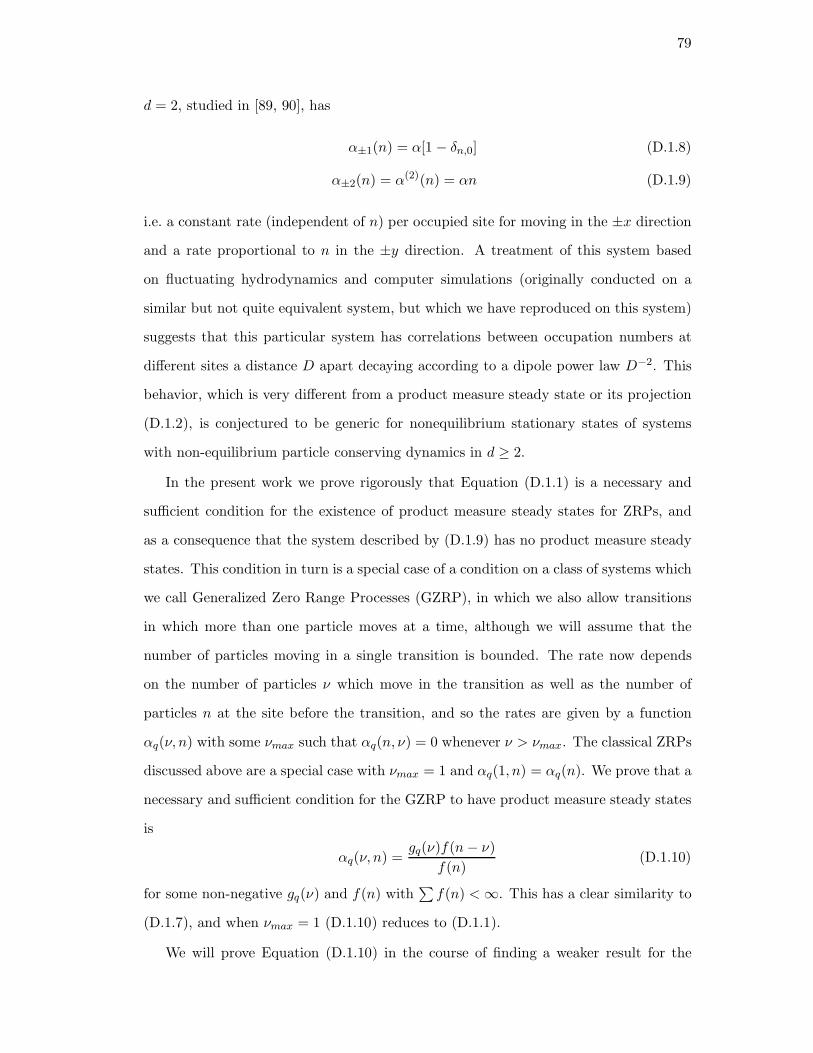
79

d = 2, studied in [89, 90], has

α±1(n) = α[1 − δn,0] (D.1.8)

α±2(n) = α(2)(n) = αn (D.1.9)

i.e. a constant rate (independent of n) per occupied site for moving in the ±x direction

and a rate proportional to n in the ±y direction. A treatment of this system based

on fluctuating hydrodynamics and computer simulations (originally conducted on a

similar but not quite equivalent system, but which we have reproduced on this system)

suggests that this particular system has correlations between occupation numbers at

different sites a distance D apart decaying according to a dipole power law D−2. This

behavior, which is very different from a product measure steady state or its projection

(D.1.2), is conjectured to be generic for nonequilibrium stationary states of systems

with non-equilibrium particle conserving dynamics in d ≥ 2.

In the present work we prove rigorously that Equation (D.1.1) is a necessary and

sufficient condition for the existence of product measure steady states for ZRPs, and

as a consequence that the system described by (D.1.9) has no product measure steady

states. This condition in turn is a special case of a condition on a class of systems which

we call Generalized Zero Range Processes (GZRP), in which we also allow transitions

in which more than one particle moves at a time, although we will assume that the

number of particles moving in a single transition is bounded. The rate now depends

on the number of particles ν which move in the transition as well as the number of

particles n at the site before the transition, and so the rates are given by a function

αq(ν, n) with some νmax such that αq(n, ν) = 0 whenever ν > νmax. The classical ZRPs

discussed above are a special case with νmax = 1 and αq(1, n) = αq(n). We prove that a

necessary and sufficient condition for the GZRP to have product measure steady states

is

αq(ν, n) =gq(ν)f(n− ν)

f(n)(D.1.10)

for some non-negative gq(ν) and f(n) with∑f(n) <∞. This has a clear similarity to

(D.1.7), and when νmax = 1 (D.1.10) reduces to (D.1.1).

We will prove Equation (D.1.10) in the course of finding a weaker result for the

80

continuous-time Mass Transport Process generalized to dimension d ≥ 1 and to transi-

tions in all directions. We show that these systems have product measure steady states

when αq(µ,m) = gq(µ)p(m − µ)/p(m). This condition is also necessary under certain

conditions (generalizing (D.1.7) to higher dimension) and we conjecture that this is so

in all cases.

D.2 Factorizability in the Mass Transport Process

Let PΛ(m, t) be the time-dependent probability density of finding the system in a par-

ticular configuration m with mass mi at site i ∈ Λ, mi ∈ (0,∞). As noted above, we are

considering periodic boundary conditions; this case is somewhat simpler than those of

other boundary conditions. The master equation describing the evolution of PΛ(m, t)

is

∂PΛ(m, t)

∂t=∑

i∈Λ

−

∑

q∈E

∫ mi

0dµαq(µ,mi)P (m, t)

+∑

q

∫ mi

0dµα−q(µ,mi+q + µ)P (mi,q,µ, t)

) (D.2.1)

where

mi,q,µj =

mj, j /∈ {i, i + q}

mj − µ, j = i

mj + µ, j = i+ q

(D.2.2)

A stationary state of the system is a distribution PΛ(m) such that ∂PΛ(m, t)/∂t = 0

whenever PΛ(m, t) = PΛ(m), or equivalently

∑

i∈Λ

∑

q

∫ mi

0dµαq(µ,mi)PΛ(m) =

∑

i∈Λ

∑

q

∫ mi

0dµα−q(µ,mi+q + µ)PΛ(m

i,q,µ) (D.2.3)

We wish to find conditions under which there is a PΛ which is factorizable, that is

which takes the form of

PΛ(m) =∏

i∈Λ

p(mi) (D.2.4)

Assuming that αq(µ,m) > 0 for all m > 0 and 0 < µ ≤ m for at least one q of each

pair of opposite directions, the system in a finite torus Λ will have a unique steady state

81

corresponding to each value of the total mass M =∑mi. Any linear combination of

such states is also a solution of (D.2.3). Given a factorizable steady state, states of

definite total mass can be obtained by projecting P onto the set of configurations with

a particular value of M in analogy with Equation (D.1.2).

Assume that there is a factorizable steady state as in (D.2.4). Let p(s) be the

Laplace transform of p(m), and let

φq(µ, s) = [1/p(s)]

∫ ∞

0dme−smαq(µ,m+ µ)p(m+ µ) (D.2.5)

Note that, since αq(µ,m) = 0 for m < µ,∫ ∞

0dme−smαq(µ,m)p(m)

= e−sµ

∫ ∞

0dme−smαq(µ,m+ µ)p(m+ µ) = e−sµφq(µ, s)p(s)

(D.2.6)

We also have∫ ∞

0dme−sm

∫ m

0dµαq(µ,m)p(m) =

∫ ∞

0dµ

∫ ∞

µdme−smαq(µ,m)p(m)

=

∫ ∞

0dµe−sµ

∫ ∞

0dme−smαq(µ,m+ µ)p(m+ µ)

=

∫ ∞

0dµe−sµφq(µ, s)p(s)

(D.2.7)

Multiplying both sides of (D.2.3) by∏

i e−simi and integrating over allmi, we obtain

∑

i∈Λ,q∈E

∏

j 6=i

p(sj)

∫ ∞

0dmi

∫ mi

0dµαq(µ,mi)p(mi)e

−simi

=∑

i∈Λ,q∈E

∏

j 6=i,i+q

p(sj)

∫ ∞

0dmi

∫ ∞

0dmi+q

∫ ∞

0dµ

× α−q(µ,mi+q + µ)p(mi − µ)p(mi+q + µ)e−simi−si+qmi+q

(D.2.8)

Rewriting (D.2.8) with the aid of (D.2.6) and (D.2.7) and canceling common factors,

we obtain∑

i∈Λ,q

∫ ∞

0dµφq(µ, si)e

−siµ =∑

i∈Λ,q

∫ ∞

0dµφ−q(µ, si+q)e

−siµ (D.2.9)

Equation (D.2.9) will be satisfied if (though not only if)

φq(µ, s) = gq(µ) (D.2.10)

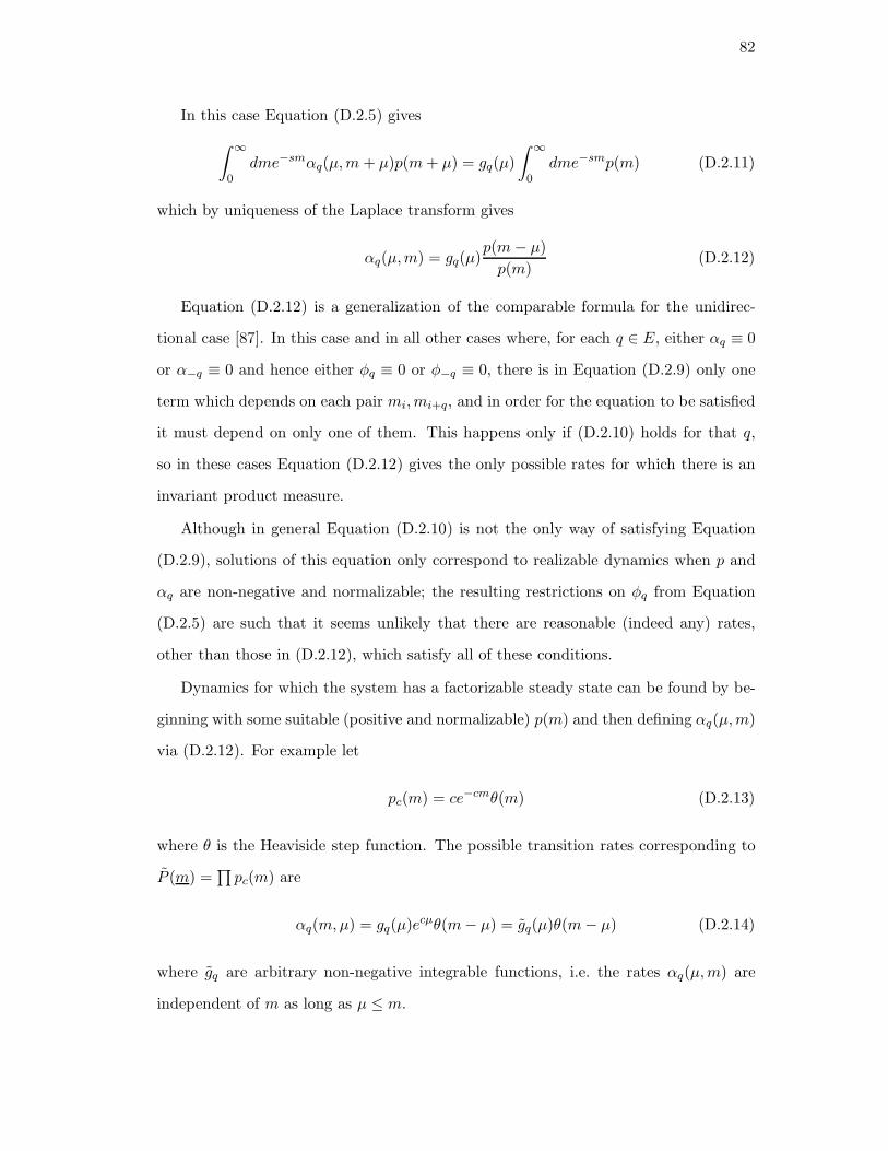
82

In this case Equation (D.2.5) gives

∫ ∞

0dme−smαq(µ,m+ µ)p(m+ µ) = gq(µ)

∫ ∞

0dme−smp(m) (D.2.11)

which by uniqueness of the Laplace transform gives

αq(µ,m) = gq(µ)p(m− µ)

p(m)(D.2.12)

Equation (D.2.12) is a generalization of the comparable formula for the unidirec-

tional case [87]. In this case and in all other cases where, for each q ∈ E, either αq ≡ 0

or α−q ≡ 0 and hence either φq ≡ 0 or φ−q ≡ 0, there is in Equation (D.2.9) only one

term which depends on each pair mi,mi+q, and in order for the equation to be satisfied

it must depend on only one of them. This happens only if (D.2.10) holds for that q,

so in these cases Equation (D.2.12) gives the only possible rates for which there is an

invariant product measure.

Although in general Equation (D.2.10) is not the only way of satisfying Equation

(D.2.9), solutions of this equation only correspond to realizable dynamics when p and

αq are non-negative and normalizable; the resulting restrictions on φq from Equation

(D.2.5) are such that it seems unlikely that there are reasonable (indeed any) rates,

other than those in (D.2.12), which satisfy all of these conditions.

Dynamics for which the system has a factorizable steady state can be found by be-

ginning with some suitable (positive and normalizable) p(m) and then defining αq(µ,m)

via (D.2.12). For example let

pc(m) = ce−cmθ(m) (D.2.13)

where θ is the Heaviside step function. The possible transition rates corresponding to

P (m) =∏pc(m) are

αq(m,µ) = gq(µ)ecµθ(m− µ) = gq(µ)θ(m− µ) (D.2.14)

where gq are arbitrary non-negative integrable functions, i.e. the rates αq(µ,m) are

independent of m as long as µ ≤ m.

83

D.3 Reverse processes

In this section we will show that Equation (D.2.12) is a necessary condition for the

existence of factorizable steady states of any MTP whose reverse process is also an

MTP. The relevant way in which the reverse process can fail to be an MTP is that it

can have transition rates which depend on the mass at the target site of the transition

as well as on the mass at the site it is leaving.

In general, given a Markov process with transition rates K(m→ m′) and stationary

distribution P (m), the reverse process is defined by rates K∗(m → m′) given by

K∗(m → m′) =K(m′ → m)P (m′)

P (m)(D.3.1)

This new process is what one obtains by running the original process backwards. Conse-

quently the reverse process has the same stationary distribution as the original process,

and when K is translation in variant so is K∗.1

For an MTP defined by rates αq(mi, µ), K(m → m′) is equal to αq(mi, µ) for

configurations m and m′ related by moving a mass µ from site i to i + q, and to 0

otherwise. The reverse process is specified by the rate function α∗i,q(µ,m) which is the

rate of transitions from a configuration m in which a mass µ moves from site i to site

i+ q; these are the only transitions in this process.

When P (m) is a product measure with single-site weights p(m), (D.3.1) becomes

α∗i,q(µ,m) = α−q(µ,mi+q + µ)

p(mi − µ)p(mi+q + µ)

p(mi)p(mi+q)(D.3.2)

Rewriting, we have

α∗i,q(µ,m)

p(mi)

p(mi − µ)= α−q(µ,mi+q + µ)

p(mi+q + µ)

p(mi+q)(D.3.3)

If α∗ defines a mass transport process, then it must be independent of all mj for j 6= i.

In this case both sides of (D.3.3) are equal to some function which depends only on µ

and q. This which can only be true if α satisfies Equation (D.2.12), in which case one

finds that

α∗i,q(µ,m) = α−q(µ,mi) (D.3.4)

1If for some configurations P (m) = 0, then one defines a new process on a configuration spaceexcluding these configurations (this problem does not arise in the case under consideration).

84

D.4 Factorizability in Generalized Zero Range Processes

With mass at each site restricted to an integer particle number ni, we can reproduce

the analysis in the previous section up to Equation (D.2.9). Denoting the vector of

occupation numbers by n, and the transition rates by αq(ν, n), the stationarity condition

corresponding to Equation (D.2.3) is

∑

i∈Λ

∑

q∈E

ni∑

ν=1

(−αq(ν, ni)PΛ(n) + α−q(ν, ni+q + ν)PΛ(n

i,q,ν))= 0 (D.4.1)

Suppose P is factorizable,

PΛ(n) =∏

i∈Λ

p(ni) (D.4.2)

where p(n) is the probability of having n particles at a given site. Then define the

generating function (discrete Laplace transform)

p(z) =

∞∑

n=0

znp(n) (D.4.3)

and let

φq(ν, z) =

∑∞n=0 z

nαq(ν, n+ ν)p(n+ ν)

p(z)(D.4.4)

Note that φq(ν, z) ≥ 0 for all ν, z ≥ 0. The counterpart of Equation (D.2.9) is then

∑

i∈Λ,q∈E

∞∑

ν=1

zνi φq(ν, zi) =∑

i∈Λ,q∈E

∞∑

ν=1

zνi φ−q(ν, zi+q) (D.4.5)

We now exploit the assumption that transitions occur only for ν ≤ νmax. Then

choosing some j ∈ Λ and q ∈ E and taking the kth derivative of the above expression

with respect to zj and zj+q gives

νmax∑

ν=k

ν!

(ν − k)!zν−kj φ

(k)−q (ν, zj+q) +

νmax∑

ν=k

ν!

(ν − k)!zν−kj+q φ

(k)q (ν, zj) = 0 (D.4.6)

For k = νmax, we have

φ(νmax)q (νmax, zj) + φ

(νmax)−q (νmax, zj+q) = 0 (D.4.7)

For (D.4.7) to hold for all zj and zj+q, both terms on the left-hand-side must be constant,

and thus the functions φ±q(νmax, ·) are polynomials of degree νmax; being non-negative

they must have non-negative leading terms. Equation (D.4.7) states that pairs of leading

85

terms of these polynomials must add up to zero and so each must be zero, and therefore

the functions φq(νmax, ·) are polynomials of degree at most νmax − 1 for each q.

Now setting k = νmax−1 we find by the same reasoning that the functions φq(νmax, ·)

are polynomials of degree at most νmax − 2. Proceeding in this manner we find

φq(ν, z) = gq(ν) (D.4.8)

as a necessary as well as a sufficient condition for (D.4.5) to be satisfied. Referring to

the definition of φ, this implies that

αq(ν, n) = gq(ν)p(n− ν)

p(n)(D.4.9)

is a necessary and sufficient condition for the existence of a product measure.

In the case where νmax = 1 and αq(1, n) = αq(n), this condition becomes

αq(n) = cqp(n− 1)

p(n)(D.4.10)

This is what we referred to above as the classical ZRP, with the well-known stationary

measure [82, 84] discussed in the introduction.

D.5 GZRPs on infinite lattices

In order to show that we have really found all of the factorizable steady states of this

class of systems, it remains to be established that the conditions obtained also apply

to an infinite lattice; that is, that there are not rates for which the resulting GZRP on

an infinite lattice has product measure steady states while the GZRPs defined on finite

lattices have none, or do not have the same such stationary states.

Let P (n) be a product measure with single-site distribution p(n) which is stationary

for rate functions α on Zd, and let Λ be a finite box in Z

d such that there is some i0 ∈ Λ

such that i0 + q ∈ Λ for all q ∈ E. Denote by nΛ the configuration of the system inside

86

of Λ, and let P (nΛ) be the marginal distribution of this configuration. Then we have

d

dtP (nΛ) =−

∑

i∈Λ

∑

q∈E

ni∑

ν=1

αq(ν, ni)P (nΛ) +∑

i∈Λ

∑

q∈E

ni+q∑

ν=1

αq(ν, ni + ν)P (ni,q,νΛ )

−∑

i∈∂Λ

∑

q∈E:i+q∈Λ

∞∑

ν=1

∞∑

n=ν

αq(ν, n)P (nΛ)p(n)

+∑

i∈∂Λ

∑

q∈E:i+q∈Λ

∞∑

n=1

n∑

ν=1

αq(ν, n)P (ni,q,νΛ )p(n)

=0

(D.5.1)

where ∂Λ = {i ∈ Zd \ Λ|(∃q ∈ E)(i+ q ∈ Λ)} and

ni,q,νk =

nk, k /∈ {i, i + q} ∩ Λ

nk + ν, k = i ∈ Λ

nk − ν, k = i+ q ∈ Λ

(D.5.2)

Equation (D.5.1) is very similar to Equation (D.4.1), and by repeating the procedure

used above with Equation (D.5.1) in place of Equation (D.4.1), it can easily be seen

that α and p must satisfy Equation (D.4.6) and so that (D.4.9) is a necessary condition

for the existence of a product measure steady state of the process on Zd as well as on

a finite torus.

D.6 Conclusion

We have shown that there is a straightforward necessary and sufficient condition, Equa-

tion (D.1.10), for a generalized Zero Range Process to have a product measure steady

state. For Mass Transport Processes, we have found a condition, Equation (D.2.9), for

the existence of a product measure steady state, which is considerably more opaque

than in the GZRP; it is not clear that this is equivalent to the sufficient condition

expressed in Equation (D.2.12), the counterpart of the condition we have obtained for

GZRPs. We have, however, presented some reasons to believe that it is.

Acknowledgements

The work of RLG was supported by Department of Education grant P200A030156-03.

The work of JLL was support by NSF grant DMR 01-279-26, and by AFOSR grant

87

AF 59620-01-1-0154. We thank P A Ferrari for a fruitful discussion at the Institut des

Hautes Etudes Scientifiques in Bures-Sur-Yvette, France, where part of this work was

done. We also thank R K P Zia for useful discussions.

88

References

[1] Y. Imry, S.k. Ma, Phys. Rev. Lett. 35(21), 1399 (1975)

[2] R. Brout, Phys. Rev. 115(4), 824 (1959)

[3] M. Aizenman, J. Wehr, Comm. Math. Phys. 130(3), 489 (1990)

[4] R.L. Greenblatt, M. Aizenman, J.L. Lebowitz, Phys. Rev. Lett. 103(19), 197201(2009)

[5] R. Greenblatt, J. Lebowitz, J. Phys. A 39, 1565 (2006)

[6] R. Peierls, M. Born, Proceedings of the Cambridge Philosophical Society 32, 477(1936)

[7] C. Pfister, Comm. Math. Phys. 79(2), 181 (1981)

[8] C. Herring, C. Kittel, Phys. Rev. 81(5), 869 (1951)

[9] J. Chalker, J. Phys. C 16, 6615 (1983)

[10] D.S. Fisher, J. Frohlich, T. Spencer, J. Stat. Phys. 34(5), 863 (1984)

[11] A. Aharony, Y. Imry, S.k. Ma, Phys. Rev. Lett. 37(20), 1364 (1976)

[12] G. Parisi, N. Sourlas, Phys. Rev. Lett. 43(11), 744 (1979)

[13] E. Pytte, Y. Imry, D. Mukamel, Phys. Rev. Lett. 46(18), 1173 (1981)

[14] H. Kogon, D. Wallace, J. Phys. A 14, L527 (1981)

[15] K. Binder, Y. Imry, E. Pytte, Phys. Rev. B 24(11), 6736 (1981)

[16] G. Grinstein, S.k. Ma, Phys. Rev. B 28(5), 2588 (1983)

[17] K. Binder, Z. Phys. B 50(4), 343 (1983)

[18] J. Villain, Journal de Physique Lettres 43(15), 551 (1982)

[19] D.P. Belanger, A.R. King, V. Jaccarino, J.L. Cardy, Phys. Rev. B 28(5), 2522(1983)

[20] U. Krey, J. Phys. C 18, 1455 (1985)

[21] J.Z. Imbrie, Phys. Rev. Lett. 53(18), 1747 (1984)

[22] J.Z. Imbrie, Comm. Math. Phys. 98(2), 145 (1985)

[23] J. Bricmont, A. Kupiainen, Phys. Rev. Lett. 59(16), 1829 (1987)

89

[24] J. Bricmont, A. Kupiainen, Comm. Math. Phys. 116(4), 539 (1988)

[25] M. Aizenman, J. Wehr, Phys. Rev. Lett. 62(21), 2503 (1989)

[26] K. Hui, A.N. Berker, Phys. Rev. Lett. 62(21), 2507 (1989)

[27] E.T. Seppala, M.J. Alava, Phys. Rev. E 63(6), 066109 (2001)

[28] P. Bleher, J. Ruiz, V. Zagrebnov, J. Stat. Phys. 84(5), 1077 (1996)

[29] U. Behn, V. Priezzhev, V. Zagrebnov, Physica A 167(2), 481 (1990)

[30] F. Dyson, Comm. Math. Phys. 12(2), 91 (1969)

[31] M. Cassandro, E. Orlandi, P. Picco, Comm. Math. Phys. 288(2), 731 (2009)

[32] A. Hartmann, U. Nowak, Eur. Phys. J. B 7(1), 105 (1999)

[33] N. Sourlas, Computer Physics Communications 121, 183 (1999)

[34] N. Fytas, A. Malakis, Eur. Phys. J. B 61(1), 111 (2008)

[35] Y. Wu, J. Machta, Phys. Rev. B 74(6), 064418 (2006)

[36] R. Fisch, Phys. Rev. B 76(21), 214435 (2007)

[37] J. Jose, L. Kadanoff, S. Kirkpatrick, D. Nelson, Physical Review B 16(3), 1217(1977)

[38] J. Tobochnik, Physical Review B 26(11), 6201 (1982)

[39] N. Mermin, H. Wagner, Phys. Rev. Lett. 17(22), 1133 (1966)

[40] N. Mermin, J. Math. Phys. 8, 1061 (1967)

[41] S. Pirogov, Y. Sinai, Theoretical and Mathematical Physics 25(3), 1185 (1975)

[42] S. Pirogov, Y. Sinai, Theoretical and Mathematical Physics 26(1), 39 (1976)

[43] R. Fisch, Arxiv preprint arXiv:1001.3397 (2010)

[44] G. Marsaglia, W. Tsang, Journal of Statistical Software 5(8), 1 (2000)

[45] D. Thomas, W. Luk, P. Leong, J. Villasenor, ACM Computing Surveys (CSUR)39(4), 11 (2007)

[46] D. Ruelle, Statistical Mechanics: Rigorous Results (W. A. Benjamin, New York,1969)

[47] B. Simon, The Statistical mechanics of lattice gases, vol. 1 (Princeton Univ. Press,1993)

[48] M. Aizenman, G. Gallavotti, S. Goldstein, J. Lebowitz, Comm. Math. Phys. 48(1),1 (1976)

[49] M. Aizenman, A. Klein, C. Newman, in Phase Transitions: Mathematics, Physics,Biology, ed. by R. Kotecky (World Scientific, 1993), pp. 129–137

90

[50] M. Aizenman, B. Nachtergaele, Comm. Math. Phys. 164(1), 17 (1994)

[51] S. Sachdev, Quantum phase transitions (Cambridge University Press, 2001)

[52] M. Campanino, A. Klein, J. Perez, Comm. Math. Phys. 135(3), 499 (1991)

[53] D.S. Fisher, Phys. Rev. Lett. 69(3), 534 (1992)

[54] T. Senthil, Phys. Rev. B 57(14), 8375 (1998)

[55] P. Goswami, D. Schwab, S. Chakravarty, Phys. Rev. Lett. 100(1), 015703 (2008)

[56] A. Bovier, Statistical Mechanics of Disordered Systems: A Mathematical Perspec-tive (Cambridge University Press, 2006)

[57] S. Barreto, F. Fidaleo, Comm. Math. Phys. 250(1), 1 (2004)

[58] F. Fidaleo, Comm. Math. Phys. 262(2), 373 (2006)

[59] O. Bratteli, D. Robinson, Operator algebras and quantum statistical mechanics. 1.C∗-and W ∗-algebras, symmetry groups, decomposition of states (Springer Verlag,1987)

[60] O. Bratteli, D. Robinson, Operator Algebras and Quantum Statistical Mechanics2: Equilibrium States, Models in Quantum Statistical Mechanics (Springer, 1997)

[61] M. Schechter, P. Stamp, J. Phys. Condens. Mat. 20, 244136 (2008)

[62] P. Vuillermot, J. Phys. A: Math. Gen 10(8), 1319 (1977)

[63] J. Lindeberg, Mathematische Zeitschrift 15(1), 211 (1922)

[64] M. Ledoux, The concentration of measure phenomenon (American MathematicalSociety, 2001)

[65] P. Hall, C. Heyde, Limit Theory and Its Applications (Academic Press, New York,1980)

[66] P. Billingsley, Probability and Measure, 2nd edn. (John Wiley and Sons, New York,1986)

[67] J. Heinonen, Lectures on analysis on metric spaces (Springer Verlag, 2001)

[68] J. Siek, L. Lee, A. Lumsdaine, The Boost Graph Library (Addison-Wesley Boston,MA, 2002)

[69] J. Picard, H. Ratliff, Networks 5, 357 (1974)

[70] L. Ford, D. Fulkerson, Canadian Journal of Mathematics 8(3), 399 (1956)

[71] P. Elias, A. Feinstein, C.E. Shannon, IRE Transactions on Information Theory2(4), 117 (1956)

[72] A. Goldberg, Tech. Mem. MIT/LCS/TM-291, Laboratory for Computer Science,MIT, Cambridge, MA (1985)

91

[73] A.V. Goldberg, R.E. Tarjan, in STOC ’86: Proceedings of the eighteenth annualACM symposium on Theory of computing (ACM, New York, NY, USA, 1986), pp.136–146

[74] A.N. Berker, Phys. Rev. B 42(13), 8640 (1990)

[75] M. Schechter, Phys. Rev. B 77(2), 020401(R) (2008)

[76] M. Schechter, P.C.E. Stamp, Phys. Rev. B 78(5), 054438 (2008)

[77] J. Wehr, A. Niederberger, L. Sanchez-Palencia, M. Lewenstein, Phys. Rev. B74(22), 224448 (2006)

[78] A. Niederberger, T. Schulte, J. Wehr, M. Lewenstein, L. Sanchez-Palencia,K. Sacha, Phys. Rev. Lett. 100(3), 030403 (2008)

[79] R.L. Greenblatt, M. Aizenman, J.L. Lebowitz, In preparation

[80] A. Klenke, Probability theory: a comprehensive course (Springer Verlag, 2008)

[81] M. Evans, T. Hanney, J. Phys. A 38(19), R195 (2005)

[82] F. Spitzer, Advances in Mathematics 5(2), 246 (1970)

[83] E. Andjel, The Annals of Probability 10(3), 525 (1982)

[84] M. Evans, Brazilian Journal of Physics 30, 42 (2000)

[85] S. Großkinsky, G. Schutz, H. Spohn, J. Stat. Phys. 113(3), 389 (2003)

[86] Y. Kafri, E. Levine, D. Mukamel, G. Schutz, J. Torok, Phys. Rev. Lett. 89(3),35702 (2002)

[87] M. Evans, S. Majumdar, R. Zia, J. Phys. A 37(25), L275 (2004)

[88] S. Majumdar, M. Evans, R. Zia, Phys. Rev. Lett. 94(18), 180601 (2005)

[89] H. van Beijeren, J. Stat. Phys. 60(5), 845 (1990)

[90] Z. Cheng, P.L. Garrido, J.L. Lebowitz, J.L. Valles, Europhysics Letters 14(6), 507(1991)

92

Vita

Curriculum Vitae

Rafael L Greenblatt

2002-2010 Ph.D. in Physics, Rutgers University

1998-2001 B.A. (High Distinction) in Mathematics and Physics, University of Cali-fornia Berkeley

1996-1998 Attended San Diego City College

2009 Teaching assistant, Department of Physics and Astronomy, Rutgers Uni-versity

2008-2009 Part time lecturer, Department of Physics and Astronomy, Rutgers Uni-versity

2006 Teaching assistant, Department of Physics and Astronomy, Rutgers Uni-versity

2005 Departmental graduate assistant, Department of Physics and Astronomy,Rutgers University

2003-2005 Department of Education GAANN fellow

2002-2003 Teaching assistant, Department of Physics and Astronomy, Rutgers Uni-versity

Publications:

• Comment on “Yang-Lee Zeros for an Urn Model for the Separation of Sand” (withJ.L. Lebowitz), Phys. Rev. Lett. 93 238901, 2004.

• Product measure steady states of generalized zero range processes (with J.L.Lebowitz), J. Phys. A 39 1565–1574, 2006.

• Rounding of First Order Transitions in Low-Dimensional Quantum Systems withQuenched Disorder (with M. Aizenman and J.L. Lebowitz), Phys. Rev. Lett. 103197201, 2009.

• Phase diagrams of systems with quenched randomness (with M. Aizenman andJ.L. Lebowitz), arXiv:0912.1251, to appear in Physica A, 2010.