Effects of Nonisothermality and Wind-Shears on the ...
46
© 2016. J. Z. G. Ma. This is a research/review paper, distributed under the terms of the Creative Commons Attribution- Noncommercial 3.0 Unported License http://creativecommons.org/licenses/by-nc/3.0/), permitting all non commercial use, distribution, and reproduction in any medium, provided the original work is properly cited. Global Journal of Science Frontier Research: F Mathematics and Decision Sciences Volume 16 Issue 3 Version 1.0 Year 2016 Type : Double Blind Peer Reviewed International Research Journal Publisher: Global Journals Inc. (USA) Online ISSN: 2249-4626 & Print ISSN: 0975-5896 Effects of Nonisothermality and Wind-Shears on the Propagation of Gravity Waves (II): Ray-Tracing Images By J. Z. G. Ma California Institute of Integral Studies, United States Abstract- We investigate the effects of the wind shears and nonisothermality on the ray propagation of acoustic-gravity waves in a nonhydrostatic atmosphere by generalizing Marks & Eckermann’s WKB ray-tracing formalism (1995: J. Atmo. Sci., 52, 11, 1959-1984; cited as ME95). Five atmospheric conditions are considered, starting from the simplest isothermal and shearfree case. In every step case a set of ray equations is derived to numerically code into a global ray- tracing model and calculate the profiles of ray paths in space and time, wavelengths and intrinsic wave periods along the rays, meanfield temperature or horizontal zonal/meridional wind speeds, as well as their gradients, and the WKB criterion parameter, . Results include, but not limited to, the following: (1) Rays in shear-free and isothermal atmosphere follow straight lines in space; both forward and backward-mapping rays are superimposed upon each other; wavelengths ( x,y,z ), as well as the intrinsic wave period ( ), keep constant versus altitude. (2) If Hines’ locally isothermal condition is applied, i.e., including the effect of temperature variations in altitude, ray traces become non-straight; however, their projections in the horizontal plane keep straight; the forward and backward ray traces are no longer overlain; and, show discernable changes but does not change. All the modulations happen at around 80-150 km altitudes. GJSFR-F Classification : MSC 2010: 76B15 EffectsofNonisothermalityandWindShearsonthePropagationofGravityWavesIIRayTracingImages Strictly as per the compliance and regulations of : δ τ λ x,y,z λ τ
Transcript of Effects of Nonisothermality and Wind-Shears on the ...

© 2016. J. Z. G. Ma. This is a research/review paper, distributed under the terms of the Creative Commons Attribution-Noncommercial 3.0 Unported License http://creativecommons.org/licenses/by-nc/3.0/), permitting all non commercial use, distribution, and reproduction in any medium, provided the original work is properly cited.
Global Journal of Science Frontier Research: F Mathematics and Decision Sciences Volume 16 Issue 3 Version 1.0 Year 2016 Type : Double Blind Peer Reviewed International Research Journal Publisher: Global Journals Inc. (USA) Online ISSN: 2249-4626 & Print ISSN: 0975-5896
Effects of Nonisothermality and Wind-Shears on the Propagation of Gravity Waves (II): Ray-Tracing Images
By J. Z. G. Ma California Institute of Integral Studies, United States
Abstract- We investigate the effects of the wind shears and nonisothermality on the ray propagation of acoustic-gravity waves in a nonhydrostatic atmosphere by generalizing Marks & Eckermann’s WKB ray-tracing formalism (1995: J. Atmo. Sci., 52, 11, 1959-1984; cited as ME95). Five atmospheric conditions are considered, starting from the simplest isothermal and shearfree case. In every step case a set of ray equations is derived to numerically code into a global ray-tracing model and calculate the profiles of ray paths in space and time, wavelengths and intrinsic wave periods along the rays, meanfield temperature or horizontal zonal/meridional wind speeds, as well as their gradients, and the WKB criterion parameter, . Results include, but not limited to, the following: (1) Rays in shear-free and isothermal atmosphere follow straight lines in space; both forward and backward-mapping rays are superimposed upon each other; wavelengths ( x,y,z ), as well as the intrinsic wave period ( ), keep constant versus altitude. (2) If Hines’ locally isothermal condition is applied, i.e., including the effect of temperature variations in altitude, ray traces become non-straight; however, their projections in the horizontal plane keep straight; the forward and backward ray traces are no longer overlain; and, show discernable changes but does not change. All the modulations happen at around 80-150 km altitudes.
GJSFR-F Classification : MSC 2010: 76B15
EffectsofNonisothermalityandWindShearsonthePropagationofGravityWavesIIRayTracingImages
Strictly as per the compliance and regulations of :
δ
τ
λx,y,z
λ
τ

Effects of Nonisothermality and Wind-Shears on the Propagation of Gravity Waves (II):
Ray-Tracing Images J. Z. G. Ma
Author:
California Institute of Integral Studies, San Francisco, CA, USA. e-mail: [email protected]
Abstract-
We investigate the effects
of the wind shears and nonisothermality on the ray propagation of acoustic-gravity waves in a nonhydrostatic atmosphere by generalizing Marks
& Eckermann’s WKB ray-tracing formalism (1995: J. Atmo. Sci., 52, 11, 1959-1984;
cited as ME95). Five atmospheric
conditions are considered, starting from the simplest isothermal and shearfree case. In every step case a set of ray equations is derived to numerically code into a global ray-tracing model and calculate the profiles of ray paths in space and time, wavelengths and intrinsic wave periods along the rays, meanfield temperature or horizontal zonal/meridional wind speeds, as well as their gradients, and the WKB criterion parameter, . Results include, but not limited to, the following: (1) Rays in shear-free and isothermal atmosphere follow straight lines in space; both forward and backward-mapping rays are superimposed upon each other; wavelengths ( ), as well as the intrinsic wave period ( ), keep constant versus altitude. (2) If Hines’ locally isothermal condition
is applied, i.e., including the effect of temperature variations in altitude,
ray traces become non-straight; however, their projections in the horizontal
plane keep straight; the forward and backward ray traces are no longer
overlain; and,
show discernable changes but does not change. All the
modulations happen at around 80-150 km altitudes. If the temperature constraint
is relaxed to the nonisothermal condition by adding the effect of temperature
gradients in
and
, the results do not exhibit perceptible differences.
(3) If the atmosphere is only isothermal, rays are violently modulated
by the zonal and meridional winds, and their shears in , as well as gradients in particularly during the 80-150 km altitudes where
and exhibit the most conspicuous modifications. More importantly, the forward
and the backward rays never propagate along the same paths. If the isothermal
condition is updated to the nonisothermal one by adding the effects of
temperature gradients in
and , modulations of the physical parameters
in 0-80 km altitudes become significant. (4) While the WKB is below
0.4 in the Hines’ model, it can be driven to close to 3 by the wind shears
and nonisothermality in realistic atmosphere. In addition to the above, features
of ray propagations under different initial wavelengths are also discussed.
I.
Introduction
1
Globa
lJo
urna
lof
Scienc
eFr
ontie
rResea
rch
V
olum
eXVI
Iss ue
e
rsion
IV
IIIYea
r20
16
37
( F)
δ
λx,y,z τ
λx,y,zτ
x, y, z t
z x, y, t λx,y,z τ
x, y, z tδ
Gravity stratifies atmosphere and modifies the propagation of acoustic wave through
a restoring force, namely, the buoyancy force, leading to the formation of acoustic-gravity wave, consisting of relatively higher-frequency acoustic and lower-frequency grav-
ity branches (Lamb 1908; 1910). This force produces atmospheric oscillations featured by
the buoyancy frequency, ωb (isothermal condition) or ωB (nonisothermal condition), also
well-known as the Brunt-Vaisala frequency, satisfying (Vaisala 1925; Brunt 1927; Eckart
1960; Hines 1960; Tolstoy 1963)
ω2b = (γ − 1)
g2
C2, or ω2
B = (γ − 1)g2
C2+
g
C2
dC2
dz(1)
Notes
© 2016 Global Journals Inc. (US)

Effects of Nonisothermality and Wind-Shears on the Propagation of Gravity Waves (II): Ray-Tracing Images
where γ is the adiabatic index; g is the gravitational constant; C is the speed of sound,
and z is the vertical coordinate of the atmospheric frame of reference.
Acoustic-gravity waves were firstly found to be responsible for ionospheric ripples (Hines
1960), a traveling disturbance in space plasmas which causes the fading of radio signals
(e.g., Mimno 1937; Pierce & Mimno 1940; Munro 1950, 1958; Martyn 1950; Toman
1955; Heisler 1958; Hooke 1968). In essence, the upward propagating waves are amplifiedby the exponential decrease in atmospheric density so as to trigger observable impulsivevertical undulations in Earth’s atmosphere, transfer momentum and energy to plasmaparticles in ionosphere, and bring about detectable variations in parameters like, electron
density (Hines 1972; Peltier & Hines 1976). This model was supported by a bulk of
experiments (e.g., Gershman & Grigor’ev 1968; Vasseur et al. 1972; Francis 1974),e.g., the ionospheric observations following nuclear detonations in the atmosphere (Hines1967; Row 1967). Tens of years of theoretical and experimental studies exposed that thepossible origin of the waves also included other natural or artificial sources like, solar-windirregularities, solar eclipses, meteors, polar and equatorial electrojets, rocket launches,thunderstorms, cold waves, tornadoes, tropical cyclones, vortexes, volcanic eruptions,tsunamis, earthquakes (e.g., Bolt 1964; Harkrider 1964; Pierce & Coroniti 1966; Cole
& Greifinger 1969; Tolstoy & Lau 1971; Francis 1975; Richmond 1978; Rottger, 1981;
Huang et al. 1985; Fovell et al. 1992; Igarashi et al. 1994; Calais et al. 1998; Wan et
al. 1998; Grigorev 1999; Sauli & Boska 2001; Fritts & Alexander 2003, Kanamori 2004).Unexpectedly, space experiments confirmed that the excited waves were intrinsically linked
to chemical processes in the airglow emissions in thermosphere, such as the hydroxyl (OH)nightglow fluctuations (e.g., Krassovsky 1972; Peterson 1979; Walterscheid et al. 1986),
the 6300 A redline (e.g., Sobral et al. 1978; Hines & Tarasick 1987; Mendillo et al. 1997;Kubota et al. 2001), and the far-ultraviolet 1356 A emission (e.g., Paxton et al. 2003;
DeMajistre et al. 2007).
The pioneer theoretical studies on acoustic-gravity waves happened during the 1950sand 1960s, when rudimentary theories and myriad effects of the waves had been investi-
gated, as recorded by Gossard & Munk (1954); Eckart (1960); Tolstoy (1963); Journal ofAtmospheric and Terrestrial Physics (1968); Georges (1968); AGARD (1972), and Fran-
cis (1975). Since then, particularly after the 1980s with the aid of ground-based and
space-based measurements (e.g., radar, GPS), the understanding on the wave physics andits role played in the interactions between atmosphere and ionosphere have been made
considerable progress (see details in, e.g., Fritts 1984,1989; Hocke & Schlegel 1996; Fritts
& Alexander 2003; Fritts & Lund 2011). The advances rely dominantly on three kinds
of approaches: (1) WKB (Wentzel-Kramers-Brillouin) approximation; (2) full-wave for-mulation; and (3) ray-tracing mapping. All of these methods intend to obtain solutionsof respective set of perturbation equations originated from the same set of Navier-Stokesequations of the atmosphere under different conditions, based on the problems concerned.
Initiated by Hines (1960), WKB modeling draws the most attention due to its effective-ness to provide the vertical profiles of atmospheric perturbations by assuming the horizon-tal components of parameters, as well as the background atmosphere, change only slowlyover the wave cycles of the vertical variations (Pitteway & Hines 1963; Einaudi & Hines
1970; Hines 1974; Beer 1974; Gill 1982; Hickey & Cole 1988; Nappo 2002; Vadas 2007),while the variation (km) of the vertical wavenumber (m) in altitude (z), km = ∂(lnm)/∂z,
38
Globa
lJo
urna
lof
Scienc
eFr
ontie
rResea
rch
V
olum
eYea
r20
16XVI
Iss u
e e
rsion
IV
III( F
)
© 2016 Global Journals Inc. (US)
Notes

Effects of Nonisothermality and Wind-Shears on the Propagation of Gravity Waves (II): Ray-Tracing Images
is much smaller than m, i.e., δ = km/m ≪ 1; for large δ, this condition was assumedbroken and waves were generally suggested reflected vertically (e.g., Marks & Eckermann
1995; cited as ME95 hereafter). The WKB approximation makes it valid to apply Taylorexpansion to the set of Navier-Stokes equations of continuity, momentum, and energy, byassuming the solutions have the form of ∼ exp[±i(kx + ly +mz − ωt) + z/(2H)], wherex and y are horizontal coordinates in the zonal and meridional directions, respectively,with corresponding wavenumbers k and l, H is the scale height, t is time, and ω is theground-relative (Eulerian) wave angular frequency (e.g., Hines 1963; Midgley & Liemohn
1966; Volland 1969; Francis 1973; Hickey & Cole 1987; Holton 1992; Fritts & Alexander
2003). Neglecting ion-drag, viscosity and molecular diffusionand using Hines’ locally isothermal atmospherebackground wind U along x and V along y, which are all shear-free in z,dispersion equation can be obtained as follows (Eckart 1960; Eckermann 1997):
Ω2 k2h + k2
z −Ω2 − f 2
C2
)
= ω2bk
2h + f 2k2
z (2)
where Ω = ω − kU − lV is the intrinsic frequency, f = 2ΩEsinφ is the Coriolis parameter
(ΩE is Earth’s rotation rate and φ is latitude), k2h = k2 + l2, k2
z = m2 + 1/(4H2).
For the dissipative terms, Pitteway & Hines (1963) took advantage of a complex disper-sion equation to confirm that they do contribute non-negligible effects at meteor heights.Besides, the shear-related Richardson number Ri was verified to provide a criterion,Ri ∼ 1/4, which is a necessary but not sufficient condition for dynamic instability; how-ever, this criterion might not rigorously apply to cases where the wind shear is tilted fromzenith or when the molecular viscosity is important (Hines 1971; Dutton 1986; Sonmor
& Klaassen 1997; Liu 2007). What is more, if more nonhydrodynamic terms (such asion-drag) are included, the complexity of solving the perturbed equations made it hard to
give as simple an expression of the dispersion relation as Eq.(2). Instead, Francis (1973);Hickey & Cole (1987) suggested a polynomial equation to demonstrate the dispersiveproperties of acoustic-gravity waves in the absence of wind shears,
∑
j DjRj = 0, where
function R in the square of the complex vertical wave number, κ = m+ i/(2H), in whichm becomes a complex; Di is complex coefficient; and j is the number of the Navier-Stokesequations. Studies showed that the mean-field winds has a filter effect on waves (Mayr et
al. 1984, 1990); and, waves of about 15-30 min periods and 200-400 km horizontal wave-lengths are able to reach as high as 300 km altitude in the presence of dissipative terms
(Sun et al. 2007). Note that the second point was in contrast with Vadas & Fritts (2004)’searlier argument that the waves above ∼200 km are often linked to auroral sources at highlatitudes.
Unlike the WKB model, the full-wave formulation provides all the solutions of theperturbed equations, not only the WKB ones, but also those that rigorously accountsfor the wave reflection. The formalism made use of the tridiagonal algorithm (Bruce et
al. 1953; Lindzen & Kuo 1969) and assumed a single monochromatic wave of the formf(z)ei(ωt−kx−ly) in an inhomogeneous atmosphere from the neutral troposphere upwardto the mesosphere (50-85 km in altitude; i.e., ionospheric D region), and to a maximumaltitude of 800 km in the F region, where f(z) is a perturbation function as a function
of z (e.g., Yeh & Liu 1974; Lindzen & Tung 1976; Hickey et al. 1997,2000; Liang et
1
Globa
lJo
urna
lof
Scienc
eFr
ontie
rResea
rch
V
olum
eXVI
Iss ue
e
rsion
IV
IIIYea
r20
16
39
( F)
)
Notes
below 200 km altitude,which is horizontally uniform with
a classical
© 2016 Global Journals Inc. (US)

Effects of Nonisothermality and Wind-Shears on the Propagation of Gravity Waves (II): Ray-Tracing Images
al. 1998; Schubert et al. 2003). Note that there was no waveforms in z. In this case, allfactors existing in realistic atmosphere can be considered, such as, height-dependent meantemperature, damping term associated with ion drag, molecular viscosity and thermalconduction, the filtering of background winds; the eddy and the molecular diffusion ofheat and momentum, etc., subject to boundary conditions. The model provided themagnitude and phase of the perturbed z-dependent temperature, pressure, horizontal andvertical wind speeds (e.g., Klostermeyer 1972a,b,c; Hickey et al., 1997, 1998, 2000, 2001;
Walterscheid & Hickey 2001; Schubert et al. 2005). The model was not only applied to
analyze Earth’s acoustic waves (Hickey et al. 2001; Schubert et al. 2005; Walterscheid
& Hickey 2005) and gravity waves (Hickey et al. 1997; Walterscheid & Hickey 2001),but also used for gravity-wave heating and cooling in Jupiters thermosphere (Hickey et
al. 2000; Schubert et al. 2003).
By contrast, ray-tracing mapping is theoretically based on the WKB approximation.It comes from Fermat’s principle in terms of Hamiltonian equations (Landau & Lifshitz
1959; Whitham 1961; Yeh & Liu 1972). In the application to acoustic-gravity waves, itformulates the spatial and temporal evolutions of a wave packet in a background windwith velocity v0, constrained by the WKB-approximated dispersion relation, ω = ω(x,k),where ω is the ground-based Eulerian or extrinsic wave frequency, x and k are the 3Dposition and wavenumber vectors, respectively (e.g., Jones 1969; Lighthill 1978; ME95;
Ding et al. 2003). After Hines (1960) suggested that the upward propagating gravitywaves can be reflected or refracted by mean-field winds, and, Thome (1968); Francis
(1973) proposed that zero and higher order gravity wave modes under different isother-mal conditions are able to travel horizontally as far as thousands of km, Cowling et al.
(1971) discussed the background wind effects on the ray paths and proposed a directionalfiltering model. The authors argued that if gravity waves go along the winds, the intrinsicfrequency is shifted downward; If the waves propagate against the winds, reflection mayappear. Yeh & Webb (1972) and Waldock & Jones (1984) confirmed the filtering effectexerted by the winds on waves in a stratified atmosphere. The reflection was found tooccur when wave propagate against wind; and, it is impossible for the waves to penetratethrough either along or against high-speed winds. These studies were extended in a widerscope. For example, Bertin et al. (1975) adopted a reverse ray-tracing model to studythe mechanism of wave excitation by wind perturbations in a jet stream bordering thepolar front. Waldock & Jones (1984) considered the diurnal variation of the wind in theray-tracing method. Zhong et al. (1995) examined the wind influence on the propagationof gravity waves in different seasons, and extended the ray-tracing simulations by includ-ing the tidal wind that has temporal and vertical variations in the study of the wavepropagation through the middle atmosphere.
Particularly, ME95 set up a generalized, 3D WKB ray-tracing model to accommodategravity waves of all frequencies in a rotating, stratified, compressible, but isothermal,nondissipative atmosphere. The nonhydrostatic model took advantage of three derivedequations in dispersion, refraction, and amplitude, where excluded were wind shears, tem-perature gradients, and time-dependent components of the mean-field parameters. Basedon Hines’ locally isothermal dispersion relation, the authors exposed that the decrease inthe horizontal wavenumber causes the reduction in the high-frequency cutoff; turbulentdamping is more important than scale-related radiative damping; and climatological plan-etary waves heavily modulate ray paths of waves launched from different longitudes. AfterME95’s contribution, Ding et al. (2003) employed the same Hines’ model and adoptedthe HWM93 wind & MSISE90 atmospheric models (Hedin 1991; Hedin et al. 1991) for
40
Globa
lJo
urna
lof
Scienc
eFr
ontie
rResea
rch
V
olum
eYea
r20
16XVI
Iss u
e e
rsion
IV
III( F
)
© 2016 Global Journals Inc. (US)
Notes

Effects of Nonisothermality and Wind-Shears on the Propagation of Gravity Waves (II): Ray-Tracing Images
a detailed investigation on the relation between the waves and the winds. They obtainedthat, in response to the directions of the winds, waves are divided into three types: cut-off,reflected, and propagating; and, the ray paths of the waves can be horizontally prolonged,vertically steepened, reflected, or critically coupled. A more recent work was done byWrasse et al. (2006) in the absence of dissipative terms. The authors followed ME95’sstudy and derived reverse ray-tracing equations to estimate the sources of the gravitywave disturbances from wave signatures observed at 23S (Brazil) and 7S (Indonesia) byairglow imagers.
However, acoustic-gravity waves are so complicated in their propagation through theatmosphere that it is important to take into account convection, wind shear, dissipation,sources of transport in heat, momentum, and constituents (Fritts & Alexaander 2003).It is thus important to develop Hines’ isothermal dispersion relation to a more generalone which is able to expose the influences of factors like temperature gradient, Coriolisforce, wind shear, molecular viscosity, thermal diffusivity, and ion-drag, in order to, onthe one hand, understand the damping mechanism and physical effects of the waves inthe coupling between atmosphere and ionosphere; on the other hand, validate and/orprovide a reference to the numerical full-wave solutions. Toward this goal, an influentialadvance has been achieved in a series of contributions on isothermal and shear-free, butdynamically viscous and thermally diffusive atmosphere by Vadas & Fritts (2001, 2004,2005, 2009). The work was recognized as the “Vadas-Fritts ray-tracing model” (cited asVF model hereafter), which consists of a near-field Fourier-Laplace integral representationfor the around the convective source region, where rays are launched with initial conditionsdeduced there, and a far-field ray-tracing mapping for the propagation of the gravity waves
binned in space-time grid cells, and the path of each ray is determined by its spectralamplitude and by the local density of rays within the grid cells (see details in Section 2
of Broutman & Eckermann 2012).
Said study improved over past efforts on WKB ray-tracing technique. Unlike usingthe traditional “complex-m approach” usually used in atmospheric physics by assuminga complex vertical wave number (mr+ imi) and a real wave frequency ω in, e.g., Pitteway
&Hines (1963), the VF model adopted a “complex-ω approach”plasma physics by incorporating a complex wave frequency (ωr + iωi) but a real m intothe dispersion relation. Otherwise, the authors claimed that the derived compressible,complex, dispersion equation, equipped with terms of molecular viscosity (ν) and thermaldiffusivity (incorporated in the Prandtl number Pr), was unable to be solved. Thoughvia a different approach, the model led to similar results as those obtained by Pitteway &Hines (1963), such as, wave damping by thermal conduction is the same order as viscousdamping; amplitude of perturbations in an inviscid atmosphere always keeps constant,in addition to the factor of 1/(2H), regardless of any positions in space; in a viscidatmosphere, the wave growth depends entirely on ν. More significantly, the authorsfound that waves in high frequencies and large vertical wavelengths will propagate tohigh altitudes, and it is the integrated viscosity effect, rather than the local value ofviscosity, that determines wave dissipation; molecular viscosity and thermal diffusivityact as filters on the wave spectrum, allowing only those high-frequency, large verticalwavelength waves to propagate up to high altitudes. The model was assumed not only tointerpret measurements such as the airglow data near 85 km altitude (Vadas et al. 2009),but also to explain the ionospheric soundings near 250 km altitude (Vadas & Crowley2010).
1
Globa
lJo
urna
lof
Scienc
eFr
ontie
rResea
rch
V
olum
eXVI
Iss ue
e
rsion
IV
IIIYea
r20
16
41
( F)
The achievements introduced above under isothermal and shear-free conditions are ofgreat importance for us to gain fundamental understandings on the physics of generalized
Notes
which is always employed in
© 2016 Global Journals Inc. (US)

Effects of Nonisothermality and Wind-Shears on the Propagation of Gravity Waves (II): Ray-Tracing Images
acoustic-gravity waves, and then, based on this knowledge, to take incremental steps forsuitable solutions of more realistic problems. Such a problem has arisen in last 15 yearssince lidar facilitates recorded both large wind shears (e.g., 100 m/s per km) and largetemperature gradient (up to 100 K per km) between ∼85 and 95 km altitudes (Liu etal. 2002; Fritts et al. 2004; Franke et al. 2005; She et al. 2006, 2009). Spaceborne dataalso confirmed that the criterion of wind-shear related Richardson number, Ri ≤ 1/4,appeared to reach 1 at 90 km altitude over Svalbard (78N, 16E; Hall et al. 2007); and,
measurements of airglow layer perturbations in O(1S) (peak emission altitude ∼97 km)
and OH (peak emission altitude ∼87 km) driven by propagating acoustic-gravity wavessuggested that the factor of 1/(2H) should be modified by (1 − β)/(2H), where β is the
so-called “damping factor” (Liu & Swenson 2003; Vargas et al. 2007). This parameteris positive, varying between 0.2 and 1.69 with a stronger positive correlation with themeridional wind shear than the zonal one, and a positive correlation for waves of shorterthan 40 km vertical wavelengths, while a negative correlation for longer ones (Ghodpage et
al. 2014). Considering the fact that both the ion drag and Coriolis force can be neglectedbelow 600 km (Volland 1969), and viscosity can also be omitted as compared with heatconductivity within the same heights, while below about 200 km the later itself turns out tobe evanescent (Harris & Priester 1962; Pitteway & Hines 1963; Volland 1969), influencesby both wind shears and nonisothermality were consequently regarded as the candidatesto exert impacts on the propagation of gravity waves through realistic mesosphere andlower thermosphere. The most recent study by Ma et al. (2014) exposed that (1) Windshears and nonisothermality modulate Hines’ model in both real and imaginary verticalwavenumbers. While negligible below 80 km altitude, the modulation is appreciable above80 km altitude. It drives the atmosphere into a “sandwich” structure with three layers:80-115 km, 115-150 km, and 150-200 km. (2) “Damping factor”, β, keeps positive inthe top and bottom layers where wave attenuations (damping effect) appear, while it isnegative in the middle layer where wave intensification (amplifying effect) occurs. Thesign of β is determined by cosθ, where θ is the angle between the mean-field wind velocityand horizontal wave vector. (3) The strongest intensification happens at 125 km altitudeat which the imaginary vertical wave-number, mi, is - 0.25 km−1; the three strongestattenuations happen at 90, 100, 180 km altitudes with mi =+0.01, +0.03, +0.05 km−1,respectively. (4) Within the acoustic and gravity wave-periods, usually no more than tensof minutes, the Coriolis effect plays an unrecognized role, whileas it affects the inertialwaves, the waveperiod of which is in the order of hours.
Therefore, the isothermal and shear-free assumptions may be inadequate to be appliedfor a quantitative explanation of the observations in much more complicated situationsin atmosphere, especially in the modeling and analyses of spaceborne data from, e.g.,RADAR, GPS. Nevertheless, we argue that the formalism underful, at least qualitatively speaking, as a good reference for us to treat realistic atmosphericsituations (e.g., Wrassea et al. 2006) where both the temperature and wind gradients inthe vertical direction are unable to be neglected, as demonstrated by the airglow measure-ments below 200 km altitude. It is thus necessary to take into account these importantfactors in ray-tracing imaging so as to have a better understanding on the propagation ofacoustic-gravity waves in the presence of nonisothermality and wind shears. This paperwill extend the VF model by incorporating the vertical temperature inhomogeneity and
perturbed set of mass, momentum, and energy equations, but adopt-ing ME95’s simplification of ignoring the dissipation terms (i.e., molecular viscosity, heat
42
Globa
lJo
urna
lof
Scienc
eFr
ontie
rResea
rch
V
olum
eYea
r20
16XVI
Iss u
e e
rsion
IV
III( F
)
© 2016 Global Journals Inc. (US)
source, ion drag). The negligence of these terms had already been validated by classicalwork of, e.g., Harris & Priester (1962); Pitteway & Hines (1963); Volland (1969). Wefollow ME95’s algebra and nomenclature by taking the traditional complex-kz approach
Notes
previous assumptions is help
wind shear into a

Effects of Nonisothermality and Wind-Shears on the Propagation of Gravity Waves (II): Ray-Tracing Images
to manipulate dispersion equation for ray-tracing equations, rather than the complex-ωalgebra used in the VF model. In order to clearly illustrate the propagating paths of3D rays driven by diverse, localized, and intermittent sources (such as, tsunami, volcano)in realistic atmosphere, we intentionally expand the inviscid heights from 0∼200 km to0∼300 km in ray-tracing simulations.
The structure of the paper is as follows. Section 2 develops ME95’s locally isothermalray-tracing model to a generalized set of ray-tracing equations of acoustic-gravity wavesunder wind-shearing and nonisothermal conditions. Section 3 presents numerical resultsof ray-tracing images in five different atmospheric situations, starting from the simplestisothermal and shear-free model to the most complicated nonisothermal and wind-shearingmodel, to expose the effects of the nonisothermality and wind shears. The vertical profileof the WKB δ parameter is also exhibited under some typical situations. Section 4 offersa quick summary and discussion. SI units are used throughout the paper, with exceptionsnoted wherever necessary.
The classical formulation of ray-tracing theory is briefly described as follows. Let ωbe the ground-based (Eulerian, or, extrinsic) wave frequency, r = x, y, z and k =k, l,mr are the position vector, and wavenumber vector, respectively, where subscript
“r” attached tom denotes the “real” part of the vertical wavenumber m. It will be omittedfor simplification throughout the rest of the text. Based on Fermat’s principle in terms of
Hamiltonian equations (e.g., Landau & Lifshitz 1959; Whitham 1961; Yeh & Liu 1972),the ray-path, Γ, of internal gravity waves are determined both spatially and temporallyby the dispersion relationship, ω = ω(r,k) (e.g., Jones 1969; Lighthill 1978):
Γ = Γ(r, t;k, ω) (3)
and m is constrained by the WKB dispersion equation along the rays:
m = m(r, t; kh, ω) (4)
For any rays with a generalized phase Φ,
Φ =∫
Γ(t)(ωdt− k · dr) (5)
only those with steady phase values are able to be observed and measured. Mathemati-
cally, this requires that the variation of Φ is zero, namely,
δΦ = δ∫
Γ(t)Gdt = δ
∫
Γ(t)ω − k ·
dr
dt
)
dt = 0 (6)
in which
G = ω − k ·dr
dt(7)
II. Ray-Tracing Equationsa) Formulation
1
Globa
lJo
urna
lof
Scienc
eFr
ontie
rResea
rch
V
olum
eXVI
Iss ue
e
rsion
IV
IIIYea
r20
16
43
( F)
is a functional to be integrated. The calculus of variations provides the following set ofdifferential equations:
)
Notes
© 2016 Global Journals Inc. (US)
Effects of Nonisothermality and Wind-Shears on the Propagation of Gravity Waves (II): Ray-Tracing Images
∂G
∂ω= 0 ,
∂G
∂k= 0 ,
∂G
∂r−
d
dt
∂G
∂rt= 0 (8)
where rt = dr/dt. Specifically, the set of vector equations is as follows:
dx
dt=
∂ω
∂k=
∂(Ω + k · v0)
∂k, or, cg = v0 + cg∗ (9)
and
dk
dt= −
∂ω
∂x= −
∂(Ω + k · v0)
∂x= −
∂(k · v0)
∂x−
∂Ω
∂x(10)
where
Ω = ω − k · v0 = ω − kh · v0, cg =∂ω
∂k, cg∗ =
∂Ω
∂k(11)
are the Doppler-shifted (Lagrangian, or, intrinsic) wave frequency, the extrinsic and in-
trinsic group velocities, respectively, in which kh = k, l and v0 = U, V, 0.
Based on Hines (1960)’s locally isothermal and shear-free dispersion relation, ME95
developed a global WKB ray-tracing model of a set of six equations to accommodate
gravity waves of all frequencies in a nonhydrostatic, rotating, stratified, and compressible
atmosphere characterized by nonuniformities which are supposed to change slowly in realspace (x, y, z), but keep constant in time (t), that is, wave period (2π/ω; tens of minutes)
≪ Earth’s daily rotation period (1/f ∼12 hours). As a result, the mean-field horizontal
wind of velocity v0 = U(x, y, z), V (x, y, z), 0 holds ∂U/∂t = ∂V/∂t = 0. The model
assumed that each ray starts from an initial spatial position of specific longitude, latitude,and altitude, and both kh and ω were supposed constant in time along ray paths due tothe condition of ∂/∂t = 0. A set of six ray equations was obtained, as given in Eq.(A3)
of ME95.
We extend ME95’s model by incorporating three additional effects: (1) nonisothermal
effect, i.e., kT 6= 0; and (2) wind-shear effects, i.e., ∂U/∂z 6= 0 and ∂V/∂z 6= 0; and, (3)
time-dependent effect, i.e., ∂/∂t 6= 0. Consequently, not only do additional terms appear
in ME95’s six equations, which are related to temperature gradient and wind shears, but
also a new equation to demonstrate the temporal dependence of wave frequency Ω comesinto being. The set of ray equations from Eqs.(9,10) are thus expressed as follows, which
generalizes ME95’s Eq.(A3):
dxdt
= U + cg∗x = U + ∂Ω∂m
∂m∂k
, dydt
= V + cg∗y = V + ∂Ω∂m
∂m∂l, dz
dt= cg∗z =
∂Ω∂m
dkdt
= −(
k ∂U∂x
+ l ∂V∂x
)
− ∂Ω∂m
∂m∂x
, dldt
= −(
k ∂U∂y
+ l ∂V∂y
)
− ∂Ω∂m
∂m∂y
,
dmdt
= −(
k ∂U∂z
+ l ∂V∂z
)
− ∂Ω∂m
∂m∂z
, dΩdt
= ∂Ω∂m
∂m∂t
(12)
b) ME95’s model and its generalization
44
Globa
lJo
urna
lof
Scienc
eFr
ontie
rResea
rch
V
olum
eYea
r20
16XVI
Iss u
e e
rsion
IV
III( F
)
© 2016 Global Journals Inc. (US)
Notes

Effects of Nonisothermality and Wind-Shears on the Propagation of Gravity Waves (II): Ray-Tracing Images
Instead of Eq.(1b) in ME95, which was rewritten from Eq.(2) in the Introduction of this
paper, the dispersion relation used in Eq.(12) is updated to the generalized expression as
given by Eq.(12) of Ma et al. (2014):
m2 =Ω2 − ω2
A
C2+ k2
h
[
ω2B − Ω2
Ω2−
1
2
ω2v
Ω2
2− γ
γ
Ω2
k2hVpVph
+1
2cos θ
)
cos θ
]
(13)
in which
ω2A = ω2
a + gkT , C2 = γ kBT0
M, ωv =
√
(
dUdz
)2+(
dVdz
)2, cos θ = kh·v0
kh√U2+V 2
Vp =ωv
kp, Vph = Ω
kh; and, ω2
a =γ2
4(γ−1)ω2b , kT = d(lnT0)
dz, kp =
d(lnp0)dz
(14)
where ωA and ωa are the nonisothermal and isothermal cut-off frequencies, respectively; kTand kp are the scale numbers in temperature and pressure, respectively; kB is Boltzmann’s
constant; T0 is the mean-field temperature; M is the mean molecular mass of atmosphere;
ωv is the synthesized wind shear; θ is the angle between kh and v0; Vp is a quasi-phase
speed related to ωv and kp, and Vph is the horizontal quasi-phase speed. Note that the
f -terms are omitted due to their negligible roles played in the band of gravity waves.
Applying Eq.(13) to Eq.(12) produces a set of generalized, nontrivial ray-tracing equations
as follows, where the algebra involved is notoriously tedious but straightforward:
dxdt
= U − A11k + A12∂U∂z, dy
dt= V − A11l + A12
∂V∂z, dz
dt= Ω2
Ω2−ω2
B
A11m
dkdt
= −(
k ∂U∂x
+ l ∂V∂x
)
− A22kc,dldt
= −(
k ∂U∂y
+ l ∂V∂y
)
− A22lc
dmdt
= −(
k ∂U∂z
+ l ∂V∂z
)
− A22mc,dΩdt
= −A21
(
k ∂U∂t
+ l ∂V∂t
)
+ A22ct
(15)
in which
A11 = (Ω2 − ω2B)ΩC
2/A0, A12 = −Ω3C2/(A0V∗)
A21 = (Ω4 − C2k2hω
2B) /A0, A22 = A12V∗
(
K2∗ − k2
g +ω2v
4V 2
ph
cos2 θ)
kc =∂(lnC)∂x
, lc =∂(lnC)∂y
, mc =∂(lnC)
∂z, ct =
∂(lnC)∂t
(16)
where
A0 = Ω4 − C2(k2hω
2B +K2
∗Ω2), V∗ = 4Vph
kh/kp2−γγ
+Vp
Vphcos θ
K2∗ = −1
4kp
ωv
Vph
(
2−γγ
+ Vp
Vphcos θ
)
cos θ
(17)
c) Ray equations under nonisothermal and wind-sheared conditions
1
Globa
lJo
urna
lof
Scienc
eFr
ontie
rResea
rch
V
olum
eXVI
Iss ue
e
rsion
IV
IIIYea
r20
16
45
( F)
)Notes
© 2016 Global Journals Inc. (US)

Effects of Nonisothermality and Wind-Shears on the Propagation of Gravity Waves (II): Ray-Tracing Images
Because sound speed C is determined by temperature T , we see that the nonisothermalT -effect is converted to C-effect. Clearly, Eq.(15) demonstrates that the gradients ofU, V, C in the 4D spacetime (3D space + 1D time) play a leading role in the developmentof the ray path x, y, z. Note that this development is also coupled with wave vector
k, l,m. It also deserves to stress here that the above ray equations are derived under theWKB assumption. As pointed out by Einaudi & Hines (1970); Gossard & Hooke (1975);and ME95, the validity of this condition can be exhibited by a criterion parameter, δ,
expressed as (e.g., ME95)
δ =1
m
∣
∣
∣
∣
∣
∂(lnm)
∂z
∣
∣
∣
∣
∣
(18)
Under isothermal and shear-free conditions, ME95 showed that for large δ (or, equiva-
lently, m → 0) when wave approaches a caustic, the WKB approximation breaks and rayintegration terminates in simulations (see ME95 for details). The feature of this parameterwill also be discussed based on our calculations.
We expose by steps the numerical calculations of ray images about the effects of wind
shears and nonisothermality on the propagation of acoustic-gravity waves, starting from
the simplest case and ending at the most complicated one. We consider following five at-mospheric models with six simulation steps to describe the atmosphere where ray-tracingimaging calculations are performed: (1) fully isothermal, and shear-free; (2) Hines’ lo-cally isothermal and shear-free; (3) nonisothermal and shear-free; (4) fully isothermal and
wind-shearing; (5) nonisothermal and wind-shearing (generalized formulation); and, (6)nonisothermal and wind-shearing (influence of initial wavelengths). Both hydrostatic andquasi-hydrostatic cases are considered in the first two situations.
This is the simplest case: U = V = 0 and T (or C) is uniform in space and constant
in time. Naturally, ∇U = ∇V = 0 and ∂U/∂t = ∂V/∂t = 0. Eqs.(15-17) reduce to the
following:
dx
dt= −A11k,
dy
dt= −A11l,
dz
dt=
1
A∗0
;dk
dt=
dl
dt=
dm
dt=
dΩ
dt= 0 (19)
where
A∗0 =
A0
mC2Ω3, A11 =
ΩC2
A0
(
Ω2 − ω2b
)
, A0 = Ω4 − C2ω2bk
2h (20)
Eqs.(19,20) provide following equation of 3D straight rays due to the invariant nature of
all the input parameters:
III. Numerical Results
a) Fully isothermal, and shear-free atmosphere
i. Hydrostatic
46
Globa
lJo
urna
lof
Scienc
eFr
ontie
rResea
rch
V
olum
eYea
r20
16XVI
Iss u
e e
rsion
IV
III( F
)
© 2016 Global Journals Inc. (US)
Notes
Effects of Nonisothermality and Wind-Shears on the Propagation of Gravity Waves (II): Ray-Tracing Images
x
k=
y
l=
z
m
ω2b
Ω2− 1
)
, along with Ω = ω (21)
where parameters k, l,m, ω,Ω, and ωb are all constant in time. We arbitrarily choosehorizontal wavelengths of λx = 350 km and λy = 50 km and illustrate the features of rayimages in Fig.1. The top panel depicts the ray path propagating in 3D space (thick line),and its three projections (thin lines) in XY/YZ/XZ planes. The two arrows indicate bothforward and backward traces, respectively, which are superimposed upon each other. Thebottom four smaller panels in the figure present the propagating length and altitude ofthe ray versus time (upper left), the vertical profiles of sound speed C (upper right), the
three wavelengths λx, λy, and λz (lower left), and, wave period τ = 2π/Ω, cut-off period
τa = 2π/ωa, and buoyancy period τb = 2π/ωb (lower right).
As displayed in the top panel, either the forward or the backward ray is a straightline. Relative to one end, the other end is 262.89 km away along x and 1840.2 km away
along y. Clearly, x/y = k/l, following Eq.(21). The lapse of time that the ray travelsbetween the two ends is given in the upper left panel of the bottom 4 small ones. It is
185 minutes, a little more than 3 hours, propagating a distance of vertically 300 km, but1840.2 km long in space. In addition, the sound speed C is given in the upper right panel,calculated by assuming T0 = 288 K. It keeps constant at different altitudes due to theisothermal condition. Furthermore, the lower left panel exposes the vertical profiles of thethree wavelengths λx, λy, and λz. All of them do not change versus height. Lastly, thelower right panel exposes the three periods which also keep the same in altitudes.
If the hydrostatic condition is relaxed to quasi-hydrostatic, that is, the wind components
are nonzero (U 6= 0 and/or V 6= 0) but uniform in space, while keeping other constraints
unchanged, Eqs.(15-17) provide
dx
dt= U − A11k,
dy
dt= V − A11l,
dz
dt=
1
A∗0
(22)
along with the same coefficients as defined by Eq.(20). Eq.(21) is thus updated as follows:
x
k − ks=
y
l − ls=
z
m
ω2b
Ω2− 1
)
, along with Ω = ω − ωs (23)
Obviously, Eq.(23) is a generalized expression of Eq.(21) to describe straight rays in space
but with shifts ks, ls, and ωs in k, l, and ω, respectively:
ks =U
A11=
Ω4 − C2ω2bk
2h
ΩC2 (Ω2 − ω2b )U ≈
k2h
ΩU, ls =
V
A11≈
k2h
ΩV, ωs = kU + lV (24)
Accordingly, regardless of the shifts, rays are still straight lines propagating in space,
similar to Fig.1.
ii. Quasi-hydrostatic
1
Globa
lJo
urna
lof
Scienc
eFr
ontie
rResea
rch
V
olum
eXVI
Iss ue
e
rsion
IV
IIIYea
r20
16
47
( F)
)
)
Notes
© 2016 Global Journals Inc. (US)

Effects of Nonisothermality and Wind-Shears on the Propagation of Gravity Waves (II): Ray-Tracing Images
If the atmosphere is hydrostatic (U = V = 0), and T (or C) is constant in time and
uniform locally (i.e., kT = 0), the set of ray equations of Hines’ model assumes can be
obtained from Eqs.(15-17) as follows:
dxdt
= −A11k,dydt
= −A11l,dzdt
= 1A∗
0
dkdt
= −A22kc,dldt
= −A22lc,dmdt
= −A22mc
(25)
where
A∗0 =
A0
mC2Ω3 , A11 =ΩC2
A0(Ω2 − ω2
b ) , A22 =Ω3C2
A0k2g , A0 = Ω4 − C2k2
hω2b
kc =∂(lnC)∂x
, lc =∂(lnC)∂y
, mc =∂(lnC)∂z
(26)
Eq.(??) produces a set of ray equations:
dx
k=
dy
l=
ω2b
Ω2− 1
)
dz
m;
dk
kc=
dl
lc=
dm
mc
, along with Ω = ω (27)
from which we see that in the horizontal x-y plane the projection of the ray trace should
be close to a straight line due to the fact that kc ∼ lc ≪ mc, leading to small changes in
both k and l, if there are, compared to m.
Fig.2 illustrates the ray features in Hines’ locally isothermal and shear-free atmospherein both forward (in blue) and backward (in red) propagations. The upper left paneldisplays the 3D traces. Clearly, the rays are no longer straight anymore, in contrastwith Fig.1. Impressively, there appear dramatic changes in the range of 85-120 km inaltitude. However, as predicted in the above, the projections of the rays in the x-y planeappear straight. The upper right panel shows a distinct difference between the forwardand backward rays in the length and time of propagation with the same 300 km heighttravelled: the forward ray flies away as long as a distance of 700 km in ∼380 min (about
6.5 hours); while the backward one has a journey of 1100 km long in ∼600 min (about
10 hours). The lower two panels expose the vertical profiles of the three wavelengths
λx, λy, & λz (left) and the three periods τa = 2π/ωa, τb = 2π/ωb, & τ = 2π/Ω (right),
respectively. Obviously, λx and λy vary little compared to λz; in addition, λz is modulated
the most between 85 and 120 km altitudes; what is more, τa and τb have peaks between85 and 100 km.
To understand the mechanism of these ray features, we plot the mean-field parametersalong ray paths in both Fig.3 and Fig.4. The former presents T0 and C (upper left panel),
dT0/dx (upper right panel), dT0/dy (lower left panel), and dT0/dz (lower right panel);
and the latter depicts ρ0 and p0 (upper left panel), dρ0/dx (upper right panel), dρ0/dy
(lower left panel), and dρ0/dz (lower right panel). It is seen that T0 (or C), rather than ρ0
b) Hines’ locally isothermal and shear-free atmosphere
i. Hydrostatic
48
Globa
lJo
urna
lof
Scienc
eFr
ontie
rResea
rch
V
olum
eYea
r20
16XVI
Iss u
e e
rsion
IV
III( F
)
© 2016 Global Journals Inc. (US)
)
Notes

Effects of Nonisothermality and Wind-Shears on the Propagation of Gravity Waves (II): Ray-Tracing Images
(or p0), is responsible for the profile of wave periods. More importantly, it is the gradients
of T0, rather than those of ρ0, that are correlated evidentally with the abnormal featuresof the ray propagations. Note that the gradients in the horizontal plane (dT0/dx anddT0/dy) is 2 or 3 orders smaller than that in the vertical direction (dT0/dz). Thus, thevertical gradient in temperature dominates the modulation.
Fig.5 draws the altitude profiles of the WKB δ parameter in the forward and backwardpropagations. The parameter is lower on average in the former case than in the lattercase. In either case, it is smaller than 1. Interestingly, in the 85-120 km altitudes, Themagnitude becomes apparently higher than that in other altitudes.
If the hydrostatic condition is relaxed to quasi-hydrostatic, that is, the wind components
are nonzero (U 6= 0 and/or V 6= 0) but uniform in space, while keeping other constraints
unchanged, Eqs.(15-17) provide
dxdt
= U −A11k,dydt
= V −A11l,dzdt
= 1A∗
0
dkdt
= −A22kc,dldt
= −A22lc,dmdt
= −A22mc
(28)
where the coefficients are those expressed in Eq.(??). This set of equations updates
Eq.(??) as follows:
dx
k − ks=
dy
l − ls=
ω2b
Ω2− 1
)
dz
m;
dk
kc=
dl
lc=
dm
mc
, along with Ω = ω − ωs (29)
in which shifts ks, ls, and ωs in k, l, and ω, respectively, are already given in Eq.(24).
Accordingly, regardless of the shifts, the profiles of rays are similar to Figs.2∼4 in thisquasi-static case.
Realistic atmosphere is nonisothermal, i.e., kT 6= 0. We therefore extend Hines’ locally
isothermal model for more generalized situation where ωa and ωb are substituted by ωA
and ωB, respectively. To save space, we just take the hydrostatic case (U = V = 0) as an
example. In this case, Eqs.(15-17) provide
dxdt
= −A11k,dydt
= −A11l,dzdt
= 1A∗
0
dkdt
= −A22kc,dldt
= −A22lc,dmdt
= −A22mc
(30)
where
A∗0 =
A0
mC2Ω3 , A11 =ΩC2
A0(Ω2 − ω2
B) , A22 =Ω3C2
A0k2g , A0 = Ω4 − C2k2
hω2B
kc =∂(lnC)∂x
, lc =∂(lnC)∂y
, mc =∂(lnC)
∂z
(31)
c) Nonisothermal and shear-free atmosphere
ii. Quasi-hydrostatic
1
Globa
lJo
urna
lof
Scienc
eFr
ontie
rResea
rch
V
olum
eXVI
Iss ue
e
rsion
IV
IIIYea
r20
16
49
( F)
)
Notes
© 2016 Global Journals Inc. (US)

Effects of Nonisothermality and Wind-Shears on the Propagation of Gravity Waves (II): Ray-Tracing Images
Eq.(30) produces a set of ray equations:
dx
k=
dy
l=
ω2B
Ω2− 1
)
dz
m;
dk
kc=
dl
lc=
dm
mc, along with Ω = ω (32)
Eqs.(30∼32) are similar to Eqs.(25∼27), respectively. Thus, the ray features in the
present nonisothermal case are basically the same as Hines’ locally isothermal case. Forexample, in the horizontal x-y plane the projection of the ray trace is straight approxi-
mately due to the fact that kc ∼ lc ≪ mc and thus k and l are nearly constant comparedto m. As introduced in the last subsection, ray features are dominantly influenced by themean-field temperature and its spatial gradients. Fig.6 presents the characteristics of raypropagation: the 3D ray traces in the upper left panel; the ray distances versus time inthe upper right panel; the three wavelengths λx, λy, & λz in the lower left panel, and the
three periods τA = 2π/ωA, τB = 2π/ωB, and τ = 2π/Ω in the lower right panel. Fig.7
displays the altitude profiles of mean-field T0 and C (upper left), dT0/dx (upper right),
dT0/dy (lower left), and dT0/dz (lower right), respectively.
Comparing Hines’ model (Figs.2 & 3) with the nonisothermal model (Figs.6 & 7) reveals
that the introduction of the new ingredient, kT , in the cut-off and buoyancy periods results
in (1) mitigated bulges of the two ray traces in the 85-120 km altitude; (2) lower speedsof ray propagation in space, e.g., Hines’ model gives an average of 1.8 km/min (about1100 km in 600 minutes), while the nonisothermal model shows 1.3 km/min (1050 kmin 800 minutes) in the backward case. However, it is subtle to discern its effects on theprofiles of wavelengths, periods, temperature (or, equivalently, sound speed), as well asthe temperature gradients.
In this case, kT = 0, but v0 6= 0, ∂v0/∂t 6= 0, and ∂v0/∂r 6= 0. Eqs.(15-17) yield
dtdz
= A0,dxdz
= A0
(
U − A11k + A12∂U∂z
)
, dydz
= A0
(
V − A11l + A12∂V∂z
)
dkdz
= −A0∆x,dldz
= −A0∆y,dmdz
= −A0∆z,dΩdz
= −A0A21∆t
(33)
where
∆x = k ∂U∂x
+ l ∂V∂x, ∆y = k ∂U
∂y+ l ∂V
∂y, ∆z = k ∂U
∂z+ l ∂V
∂z, ∆t = k ∂U
∂t+ l ∂V
∂t
A0 =A00
mC2Ω3 , A11 =ΩC2(Ω2−ω2
b)A00
, A12 =ηΩ3C2/∆z
A00, A21 =
Ω4−C2k2hω2
b
A00
(34)
in which A00 = Ω4 − C2(ω2bk
2h + ηΩ2) and η = (1− γ/2) g∆z/(2ΩC
2)−∆2z/(4Ω
2).
Under the isothermal condition, Figs.8∼11 display the heavy impacts of wind shears onthe characteristics of ray propagation. In Fig.8, the upper left panel is the 3D ray traces.Both the forward and backward rays are wriggling through the 3D space by following twodifferent paths. The difference is obviously shown in the upper right panel: the forward
d) Fully isothermal and wind-shearing atmosphere
50
Globa
lJo
urna
lof
Scienc
eFr
ontie
rResea
rch
V
olum
eYea
r20
16XVI
Iss u
e e
rsion
IV
III( F
)
© 2016 Global Journals Inc. (US)
ray (in blue) travels ∼530 km in about 380 minutes between the sea level and the 300 kmaltitude, while the backward ray (in red) hikes around 750 km in about 320 minutes. The
)
Notes

Effects of Nonisothermality and Wind-Shears on the Propagation of Gravity Waves (II): Ray-Tracing Images
lower two panels of the figure present the wave lengths and intrinsic wave periods of thepropagation, respectively. In the LHS panel, λy appears constant in altitude, relatively
speaking, and does λz except the heights of 100-150 km. The altitude dependance of λx
in the LHS panel is similar to that of τ in the RHS panel: (1) below 80 km altitude they
keep roughly unchanged. (2) λx and τ stabilize with their respective minimum values in120-135 km altitude in the forward propagation, while with maximum values in 130-145km altitude in the backward propagation. The two arrow lines label these values. (3)above 200 km altitude, the forward parameters increase monotonously and the backwardones do not change anymore.
Along ray paths the altitude profiles of the mean-field zonal wind U and meridional wind
V are described in the upper left and upper right panels in Fig.9, respectively. The WKBδ parameter is given in the lower panel. Below 80 km altitude and above 200 km altitudeboth U and V are either unchanging or vary quasi-linearly. On the contrary, between thetwo altitudes, they exhibit oscillatory features with both positive and negative speeds. Asfar as δ, most of its amplitudes are smaller than 1, while in 100-150 km altitudes thereare a couple of peaks for both forward and backward situations, respectively. Betweenthe peaks of each pair, there exists zero-δ heights of 120-135 km in the forward case andof 130-145 km in the backward case. The two zero-δ slots correspond to the two zones ofthe minimum λx and τ values, respectively, in the lower two panels of Fig.8. Note that δcan be as high as 8, which is larger than 1, for regular ray propagation as exposed in theupper left panel of Fig.8.
The altitude profiles of the mean-field wind gradients in temporal coordinate t and
spatial ones (x, y, z) are illustrated in Figs.10 and Fig.11. The gradients in U and V havefollowing characteristics: (1) The magnitude of all the U -gradients is larger than that ofthe V -gradients, particularly below 50 km altitude where the V -gradients are nearly zero.
(2) While d(U, V )/dt ∼ several m/s per hour in magnitude, d(U, V )/dx ∼ d(U, V )/dy ≪
d(U, V )/dz ∼ several m/s per km in magnitude. This indicates that it is the wind shears
(horizontal wind velocity gradients in altitude), rather than its gradients in the horizontal
plane, that play the dominant role to influence wave propagation in atmosphere. (3)Below 80 km and above 200 km altitudes, all the wind gradients are smaller than thatbetween the two altitudes. This reminds us that the effects of the wind gradients on wavepropagation cannot not be omitted, especially in the middle atmosphere.
To adopt kT 6= 0 by relaxing the constraint of kT = 0 in the above Subsection, Eqs.(15-
17) gives rise to the most generalized set of ray-tracing equations as follows:
dtdz
= A0,dxdz
= A0
(
U −A11k + A12∂U∂z
)
, dydz
= A0
(
V −A11l + A12∂V∂z
)
dkdz
= −A0 (∆x + A22Cx) ,dldz
= −A0 (∆y + A22Cy) ,dmdz
= −A0 (∆z + A22Cz)
dΩdz
= −A0 (A21∆t − A22Ct)
(35)
e) Nonisothermal and wind-shearing atmosphere: Generalized formulation
1
Globa
lJo
urna
lof
Scienc
eFr
ontie
rResea
rch
V
olum
eXVI
Iss ue
e
rsion
IV
IIIYea
r20
16
51
( F)
where ∆x,y,z,t are expressed in Eq.(34), and,
Notes
© 2016 Global Journals Inc. (US)
Effects of Nonisothermality and Wind-Shears on the Propagation of Gravity Waves (II): Ray-Tracing Images
Cx = 1C
∂C∂x, Cy =
1C
∂C∂y, Cz =
1C
∂C∂z, Ct =
1C
∂C∂t;
A0 =A00
mC2Ω3 , A11 =ΩC2(Ω2−ω2
B)A00
, A12 =ηΩ3C2/∆z
A00,
A21 =Ω4−C2k2
hω2
B
A00, A22 =
Ω3(ω2
A−C2K2−
∆2zC
2
4Ω2)
A00
(36)
in which A00 = Ω4 − C2(ω2Bk
2h + ηΩ2) and η keeps the same as that attached to Eq.(34).
In addition to the effects of the mean-field wind, this generalized case takes into consid-eration the influences of altitude-dependent temperature, as well as the density (and thusthe pressure), and their gradients in time and space on the ray propagation. Figs.12∼17illustrate the results. In comparison with that of Fig.8, the upper left panel of Fig.12
exhibits a less wriggling feature in both forward and backward propagations. The upper
right panel shows that, while the forward ray (in blue) passes ∼400 km in about 250
minutes between the sea level and the 300 km altitude, the backward one (in red) spends
about 380 minutes to fly back to the sea level after a ∼800 km journey. The speed of the
former (400/250≈1.6 km/min) is higher than that in Fig.8 (530/380≈1.4 km/min), whilethe speed of the latter (800/380≈2.1 km/min) is approximately the same as that in Fig.8(750/320≈2.3 km/min). In addition, the altitude profiles of both the three wavelengths(lower left panel) and the intrinsic wave period (lower right panel) demonstrate that be-low 150 km nonisothermality results in stronger fluctuations in comparison with Fig.8,especially lower than 100 km altitude. Interestingly, the forward wave period is shorterthan the backward one in Fig.12 at most altitudes, in contrast to the fact that it is alwayslonger than that in Fig.8.
In Fig.13, the upper panel portrays the altitude profiles along ray paths of WKB δ. The
parameter is smaller than 0.2 above 160 km altitude. Below the altitude, the forward δis larger than the backward one between 130 km and 160 km; but it always is smallerbelow 130 km. This is different from the results given in Fig.9, where the the forward δis usually larger than the backward one, particularly in the 100-150 km altitude. Withrespect to the mean-field zonal wind (lower left panel) and the meridional wind (lowerright panel), the profiles in Fig.13 are similar to those in Fig.9.
Figs.14 & 15 draw the altitude profiles of density gradients (LHS panels) and tempera-
ture gradients (RHS panels) in t, x, y, and z. Except the t-related ones, these structures
reproduce those presented in Figs.3 & 4, respectively, with the same order of magnitudes.For dρ0/dt and dT0/dt, their appearances follow the patterns of their respective families,
but with different units of each. In addition, Figs.16 & 17 delineate the altitude profiles
of zonal wind gradients (LHS panels) and meridional ones (RHS panels) in t, x, y, and z.
The figures do not disclose discernable changes from those given in 10 & 11, respectively.
In the above Subsections, we arbitrarily selected the same group of initial horizontalwavelengths, λx0 = 350 km and λy0 = 50 km, to exhibit the features of the ray propagationunder different acoustic-gravity wave modes. In this Subsection, we choose several groupsof initial horizontal wavelengths to exhibit the influence of the parameter on the raypropagation (taking the forward situation as an example) in the generalized nonisothermal
f) Nonisothermal and wind-shearing atmosphere: Influence of initial wavelengths
52
Globa
lJo
urna
lof
Scienc
eFr
ontie
rResea
rch
V
olum
eYea
r20
16XVI
Iss u
e e
rsion
IV
III( F
)
© 2016 Global Journals Inc. (US)
and shearing mode. The considered wavelengths include following two groups of pairs:
(1) λx0, λy0 = 2π × 350, 2π × 50, 2π × 350,−2π × 50, −2π × 350, 2π × 50,
Notes
Effects of Nonisothermality and Wind-Shears on the Propagation of Gravity Waves (II): Ray-Tracing Images
−2π × 350,−2π × 50; and (2) λx0, λy0 = 2π × 50, 2π × 350, 2π × 50,−2π × 350,
−2π × 50, 2π × 350, −2π × 50,−2π × 350, where the unit of all the parameters are
in km, and the negative values represent the propagating direction of the related wavecomponents is in the reverse direction of the coordinate in the frame of reference. In thesimulation, the initial extrinsic wave period ω keeps unchanged at 30 minutes.
Fig.18 demonstrates the ray paths in space with these two groups of initial wavelengths.In each group, the four cases are discriminated by four different colors (black, blue, red,and green), respectively. Several distinct features of the ray propagation are exposed byboth the upper and lower panels of the figure: (1) All the rays propagate in space alongnon-straight paths in a quadrant determined by, and opposite to, the initial wave vectors,
respectively, in the horizontal plane, k0 = 2π/λx0, l0 = 2π/λx0. For example, in the
two panels, the ray in black (λx0 > 0 and λy0 > 0) is oriented to evolve in the thirdquadrant (x < 0 and y < 0); similarly, the ray in blue (λx0 > 0 and λy0 < 0) is in the
second quadrant (x < 0 and y > 0). (2) In the horizontal plane, the ratio between thex-displacement, ∆x, and the y-displacement, ∆y, of any projected ray paths is in the sameorder of that of the corresponding wavenumbers. For instance, the ray in red in the upperpanel has a ratio of ∆x/∆y ≈ 45/270 = 0.16 while the wavenumber ratio is k0/l0 = 0.14;
also, the ray in black in the lower panel has a ratio of ∆x/∆y ≈ 320/40 = 8 while the
wavenumber ratio is k0/l0 = 7. (3) Between 80 km and 150 km altitude all rays experiencethe most serious modulations. According to the analysis in the previous Subsections, theseinfluences are exerted dominantly by the mean-field wind components and their shears.
(4) By comparison with the upper left panel of Fig.12, these modulations caused by the
wind components and their shears become mitigated if the horizontal wavelengths are
longer, as shown in the upper panel of Fig.18.
Fig.19 portrays the temporal features of both the ray length (thick lines) and the ver-tical increments (thin lines) in the above two groups of the wave propagations. All theray paths are approximately proportional to time, with a propagation speed of 15∼18km/min in space: the upper panel gives 400/23≈17 km/min (black), 400/26≈15 km/min
(blue), 400/27≈15 km/min (red), and 400/25=16 km/min (green); and the lower panel
presents 450/32≈14 (black), 400/22≈18 km/min (blue), 360/20=18 km/min (red), and
400/25=16 km/min (green). Relatively, the vertical propagation speed is lower, around
9∼15 km/min, if assuming a linear relation between the height and time. These speedsare much higher than those obtained from the upper right panel of Fig.12: it is merelyno more than 2 km/min for the four traces. Thus, rays with longer initial horizontalwavelengths travel faster. In fact, all the rays in Fig.19 reach heights of 300-400 km inonly no more than 30 minutes; by contrast, those in Fig.12 arrive 300-800 km altitudesafter more than 260 minutes.
Fig.20 displays the development of the wavelengths λx (upper left panel), λy (upper right
panel), λz (lower left panel), and the intrinsic wave period τ (lower right panel) along the
ray paths in the two groups of wave propagations. The most conspicuous feature stays inthe modulations of the four parameters below 200 km altitude, particularly at the height
of 100-150 km. By checking Fig.19 we know this corresponds to 80-120 km altitude, themost extreme changing region of both the mean-field temperature (Fig.7,14,15) and zonal& meridional winds (Fig.13,16,17). Besides, for the horizontal wavelength (λx or λy; the
1
Globa
lJo
urna
lof
Scienc
eFr
ontie
rResea
rch
V
olum
eXVI
Iss ue
e
rsion
IV
IIIYea
r20
16
53
( F)
upper two panels in the two groups), its magnitude becomes higher than the initial value
Notes
© 2016 Global Journals Inc. (US)

(λx0 or λy0) if the value is positive, i.e., the initial wave vector component is in the x(or y) direction. For example, in the upper right panel in the first group, the red curve
denotes the case of λy0 = 2π × 50 > 0 km. Along the ray, λy increases and peaks at 150
km distance along the ray with 51.2 km. By contrast, if λx0 (or λy0) is negative, i.e., theinitial wave vector component is opposite to the x (or y) direction, the magnitude of λx
(or λy) decreases. See the green curve in the upper right panel in the second group. Inthis case, λy0 = −2π × 350 < 0 km. Along the ray, | λy | decreases to 300 km at about100 km distance along the ray.
However, the vertical wavelength, λz, behaves differently as exhibited by the two lowerleft panels in the two groups. Irrelevant to the directions of initial horizontal wavevectors,the upward propagating waves have negative λz. Its magnitude starts at λz0 = 2π×12 km.After a surprising drop of λz/(2π) to below 8 km in within 20 km ray path, it undergoes
a large swing between 3 and 8 km in the first group, and between 3 and 11 km in thesecond group, before stabilizing at 3-5 km and 3-9.5 km, respectively, after a journey of300 km long in the ray propagation. These final values correspond to λz ∼ 20-60 km.
Impressively, the wave period τ has a similar trend as shown in the two lower right panelsof the two groups: it decreases sharply at first, then goes up and down, and recoversfinally to stabilize at a period which diverge only within 1 minute (the first group) and 2minutes (the second group) from the initial values, respectively. Because the initial perodis 30 minutes, we may neglect this divergence in dealing with measurements, that is, thewave period can be assumed constant in wave propagations.
Since the 1960s, the influence of mean-field properties (such as zonal and meridionalwinds, background temperature) on the propagation of atmospheric acoustic-gravity waveshas become one of the important topics in space physics. The related ray-tracing tech-nique has also been developed to investigate gravity wave propagation under the effectsof background wind and temperature variations. Due to the importance of an accuratedescription of mean-field properties and their effects in the clarification of the observedwave-driven phenomena in atmosphere (e.g., Hickey et al. 1998), we first of all took intoaccount the wind-shearing and nonisothermal effects, as well as the Coriolis effect, to ex-tend Hines’ locally isothermal and shear-free model to describe the modes of generalizedinertio-acoustic-gravity waves under different situations below 200 km altitude, where alldissipative terms (such as viscosity and heat conductivity) (Ma et al.2014). The obtained dispersion relation recovers all the known atmospheric wave modes.
In this paper, we used the generalized dispersion relation to investigate the effects of thewind shears and nonisothermality on the ray propagation of acoustic-gravity waves. Thederived general set of ray equations not only reproduces ME95’s derivations under Hines’locally isothermal and shear-free conditions, but also provides the equation to describethe time-dependent variation of the intrinsic wave frequency. Our ray-tracing simula-tions accommodate five different types of atmospheric models, starting from the simplestsituation to the most complicated one: (1) fully isothermal, and shear-free atmosphereunder both hydrostatic and quasi-hydrostatic conditions; (2) Hines’ locally isothermal andshear-free atmosphere under both hydrostatic and quasi-hydrostatic conditions; (3) non-isothermal and shear-free atmosphere under hydrostatic conditions; (4) fully isothermaland wind-shearing atmosphere; (5) nonisothermal and wind-shearing atmosphere (gener-
alized formulation; influence of initial wavelengths). In every step, a set of ray equations
IV. Summary and Discussion
Effects of Nonisothermality and Wind-Shears on the Propagation of Gravity Waves (II): Ray-Tracing Images
54
Globa
lJo
urna
lof
Scienc
eFr
ontie
rResea
rch
V
olum
eYea
r20
16XVI
Iss u
e e
rsion
IV
III( F
)
© 2016 Global Journals Inc. (US)
was derived to numerically code into a global ray-tracing model andof ray traces in space and time; that of the wavelengths and intrinsic wave periods along
Notes
were neglected (
calculate the profiles
the ray paths; that of the mean-field density, pressure, or temperature and the horizontalwinds, as well as their gradients if available; and that of the WKB criterion parameter, δin a few typical cases.
Our studies demonstrated the influences of wind shears and atmospheric nonisother-mality on the ray propagation. In an isothermal and shear-free atmosphere, ray pathsfollow straight lines in space and time; both forward and backward-mapping traces aresuperimposed upon each other; wavelengths (λx,y,z), as well as the intrinsic wave period(τ), keep constant versus altitude. If Hines’ locally isothermal condition is applied, i.e.,including the effect of the altitude-dependent temperature, rays become non-straight spa-tially, but their projections in the horizontal plane keep straight. In this case, the forwardand backward rays are no longer overlain, and λx,y,z give discernable changes but τ doesnot change. All the obvious variations happen in 80-150 km altitude. If the temperatureconstraint is relaxed to the nonisothermal condition by adding the effect of temperaturegradients in x, y, z and t, the results do not exhibit perceptible difference. In the presenceof wind shears, as well as zonal and meridional wind gradients in space and time, but theatmosphere keeps isothermal, ray paths are violently modulated, particularly at 80-150km altitude where λx,y,z and τ exhibit striking variations. More importantly, the forwardrays and the backward ones never propagate along the same paths. If the nonisothermalcondition is employed by considering the effects of temperature variations in x, y, z andt, the modulations at 0-80 km altitude also become obvious. As far as the WKB δ pa-rameter, though it is smaller than 0.4 in Hines’ locally isothermal model, in agreementwith ME95’s estimation, it can be driven to close to 3 by the wind shears and nonisother-mality. Lastly, we found that longer initial horizontal wavelengths bring about mitigatedmodulations to ray paths and faster speeds in ray propagation.
We stress that ME95’s ray-tracing model is based on the dispersion relation derived fromHinesME95’s formulation to obtain a generalized set of ray-tracing equations by taking intoaccount the effects of wind shears and atmospheric nonisothermality on the ray propaga-tion. The focus of this paper is to illustrate the influences of the effects on acoustic-gravitywaves travelling from sea level to 200 km altitude within which the dissipation terms canbe reasonably neglected. We therefore pay attention dominantly to the waves which areable to penetrate atmosphere and reach the ionospheric height above 80 km altitude,with little energy attenuation, and ignore those waves which are either reflected or in thecut-off region (for details of the wave features in these two cases see, e.g., Ding et al.
2003). Naturally, we avoid to consider such terms related to, e.g., WKB violation, wavesaturation or damping, energy attenuation or intensification, dynamical and convectiveinstabilities, which are of little relevance to our study. Instead, we concentrate on thewaves which are capable of survival from every damping process during their propaga-tions upward from the sea level to some
suitable to provide a reference for data-fit modeling studieswith measurements in space, e.g., mesosphere and/or troposphere, where information ofthe background wind and temperature profiles are available, owing to the fact that theclose relationship between the ray paths and the mean-field atmospheric properties canbe demonstrated more evidently than before via the approach provided in the text.
V. Acknowledgments
Effects of Nonisothermality and Wind-Shears on the Propagation of Gravity Waves (II): Ray-Tracing Images
1
Globa
lJo
urna
lof
Scienc
eFr
ontie
rResea
rch
V
olum
eXVI
Iss ue
e
rsion
IV
IIIYea
r20
16
55
( F)
Notes
model. By contrast, our study expendslocally isothermal and shear- free
Thus, the resultheights.observationalshown in this paper are
The Fortran code and simulation data in this paper are available on request to John.
© 2016 Global Journals Inc. (US)

References Références Referencias
1.
AGARD (1972), Effects of Atmospheric Acoustic Gravity
Waves on Electromagnetic
Wave Propagation, Conf. Proc., 115, Harford House, London. 2.
Beer, T. (1974), Atmospheric Waves, John Wiley, New York.
3.
Bertin, F., J. Testud, and L. Kersley (1975), Medium scale gravity waves in the ionospheric F-region and their possible origin in weather disturbances, Planet. Space Sci., 23, 493-507.
4.
Bolt, B. A. (1964), Seismic air waves from the great 1964 Alaska earthquake, Nature, 202, 1095-1096.
5.
Broutman, D., and S. D. Eckermann (2012), Analysis of a ray-tracing model for gravity
waves generated by tropospheric convection, J. Geophys. Res., 117, D05132,
doi:10.1029/2011 JD016975.
6.
Bruce, C. H., D. W. Peaceman, H. H. Rachford, and J. P. Rice (1953), Calculations of unsteady-state gas flow through porous media, J. Petrol. Tech., 5, 79-92.
7.
Brunt, D. (1927), The period of simple vertical oscillations in the atmosphere, Quart. J.
Royal Meteor.
Soc., 53, 30-32. 8.
Calais, E., J. B. Minster, M. A. Hofton, and M. A. H. Gedlin (1998), Ionospheric signature of surface mine blasts from global positioning system measurements, Geophys. J.
Int., 132, 191-202. 9.
Cole, J. D., and C. Greifinger (1969), Acoustic-gravity waves from an energy source at the ground in an isothermal atmosphere, J. Geophys. Res., 74, 3693-3703.
10.
Cowling, D. H., H. D. Webb, and K. C. Yeh (1971), Group rays of internal gravity waves
in a wind-stratified atmosphere, J. Geophys. Res., 76, 213-220. 11.
DeMajistre, R., L. J. Paxton, and D. Bilitza (2007), Comparison of ionospheric measurements made by digisondes with those inferred from ultraviolet airglow, Adv. Space Res., 39,
918-925. 12.
Ding, F., W. X. Wan, and H. Yuan (2003), The influence of background winds and
attenuation on the propagation of atmospheric gravity waves, J. Atmos. and Solar-Terr. Phys., 65, 857-869.
13.
Dutton, J. A. (1986), The Ceaseless Wind, Dover, New York.
Effects of Nonisothermality and Wind-Shears on the Propagation of Gravity Waves (II): Ray-Tracing Images
14. Eckart, C. (1960), Hydrodynamics of oceans and atmospheres, Pergamon, New York.
15. Eckermann, S. D. (1997), Influence of wave propagation on the Doppler spreading ofatmospheric gravity waves, J. Atmos. Sci., 54, 2554-2573.
16. Einaudi, F. and Hines, C. O. (1970), WKB approximation in application to acousticgravity waves, Can. J. Phys., 48, 14581471.
17. Fovell, R., D. Durran, J. R. Holton (1992), Numerical simulations of convectively generated stratospheric gravity waves. J. Atmos. Sci., 49, 1427-.
18. Francis, S. H. (1973), Acoustic-gravity modes and large-scale traveling ionospheric disturbances of a realistic, dissipative atmosphere, J. Geophys. Res., 78, 2278-2301.
19. Francis, S. H. (1974), A theory of medium-scale traveling ionospheric disturbances, J. Geophys. Res., 79, 5245-5260.
20. Francis, S. H. (1975), Global propagation of atmospheric gravity waves: a review. J.Atmos. Terr. Phys., 37, 10111030, IN9, 10311054.
21. Franke, S. J., X. Chu, A. Z. Liu, and W. K. Hocking (2005), Comparison of meteor radar and Na Doppler lidar measurements of winds in the mesopause region above Maui, HI, J. Geophys. Res., 110, D09S02, doi:10.1029/2003JD004486.
22. Fritts, D. C. (1984), Gravity wave saturation in the middle atmosphere: A review oftheory and observations, Rev. Geophys. Space Phys., 22, 275-308.
56
Globa
lJo
urna
lof
Scienc
eFr
ontie
rResea
rch
V
olum
eYea
r20
16XVI
Iss u
e e
rsion
IV
III( F
)
© 2016 Global Journals Inc. (US)
Notes
23.
Fritts, D. C. (1989), A review of gravity wave saturation processes, effects, and variability
in the middle atmosphere, Pure Appl. Geophys., 130, 343-371. 24.
Fritts, D. C., and M. J. Alexander (2003), Gravity wave dynamics and effects in the
middle atmosphere, Rev. Geophys., 41, 1003, doi:10.1029/2001RG000106.
25.
Fritts, D. C., and T. S. Lund (2011), Gravity wave influences in the thermosphere and ionosphere: Observations and recent modeling, in: Aeronomy of the Earths Atmosphere
and Ionosphere, ed.: Abdu,
M. A., Pancheva, D., and Bhattacharyya, A., Springer, 109-130.
26.
Fritts, D. C., B. P. Williams, C. Y. She, J. D. Vance, M. Rapp, F.-J. L¨ubken,
A. Mullemann, F. J. Schmidlin, and R. A. Goldberg (2004), Observations
of extreme temperature and wind gradients
near the summer mesopause during the MaCWAVE/MIDAS rocket campaign, Geophys. Res. Lett., 31, L24S06,
doi:10.1029/2003GL019389. 27.
Georges, T. M. (1968), Acoustic-gravity waves in the atmosphere, Symposium Proceedings, U .S. Government Printing Office, Washinton, D. C.
28.
Gershman, B. N., and G. I. Grigor’ev (1968), Traveling ionospheric disturbances–A review,
Izv. Vyssh. Ucheb. Zaved. Radiofizika
(Engl. Transl.), 11, 5-27. 29.
Ghodpage, R. N., A. Taori, P. T. Patil, S. Gurubaran, A. K. Sharma, S. Nikte, and D. Nade (2014), Airglow measurements of gravity wave propagation and damping
over
Kolhapur (16.5N, 74.2E), Intern.
J. Geophys., 2014, ID514937, 1-9. 30.
Gill, A. E. (1982), Atmosphere-ocean dynamics. Academic Press, Orlando, FL, International Geophysics Series.
31.
Gossard, E. E., and
W. H. Munk (1954), On gravity waves in the atmosphere, J.
Meteorol., 11, 259-269.
32.
Grigorev, G. I. (1999), Acoustic-gravity waves in the Earth’s atmosphere (review). Radio- phys. Quant. Electron., 42, 3-25.
33.
Hall, C. M., T. Aso, and M. Tsutsumi (2007), Atmospheric stability at 90 km, 78N,
16E, Earth Planets Space, 59, 157-164.
1
Globa
lJo
urna
lof
Scienc
eFr
ontie
rResea
rch
V
olum
eXVI
Iss ue
e
rsion
IV
IIIYea
r20
16
1
( F)
Effects of Nonisothermality and Wind-Shears on the Propagation of Gravity Waves (II): Ray-Tracing Images
34. Harkrider, D. G. (1964), Theoretical and observed acoustic-gravity waves from explosive sources in the atmosphere, J. Geophys. Res., 69, 5295-5321.
35. Harris, I. and W. Priester (1962), Time dependent structure of the upper atmosphere, J. Atmos. Sci., 19, 286-301.
36. Hedin, A. E. (1991), Extension of the MSIS thermosphere model into the middle andlower atmosphere, J. Geophys. Res., 96, 11591172.
37. Hedin, A. E., M. A. Biondi, R. G. Burnside, G. Hernandez, R. M. Johnson, T. L. Killeen, C. Mazaudier, J. W. Meriwether, J. E. Salah, R. J. Sica, R. W. Smith, N. W. Spencer, V. B. Wickwar, T. S. Virdi (1991). Revised global model of thermosphere winds using satellite and ground-based observations. J. Geophys. Res., 96, 7657-7688.
38. Hedin, A. E., E. L. Fleming, A. H. Manson, F. J. Schmidlin, S. K. Avery, R. R. Clark, S. J. Franke, G. J. Fraser, T. Tsuda, F. Vial, and R. A. Vincent (1996), Empirical wind model for the upper, middle and lower atmosphere, J. Atmos. Terr. Phys. 58, 1421-1447.
39. Heisler, L. H. (1958), Anomalies in ionosonde records due to travelling ionospheric disturbances, Aust. J. Phys., 11, 79-90.
40. Hickey M. P., and K. D. Cole (1987), A quantic dispersion equation for internal gravity waves in the thermosphere, J. Atmos. Terr. Phys., 49, 889-899.
1
Globa
lJo
urna
lof
Scienc
eFr
ontie
rResea
rch
V
olum
eXVI
Iss ue
e
rsion
IV
IIIYea
r20
16
57
( F)
Notes
© 2016 Global Journals Inc. (US)
41.
Hickey M. P., and K. D. Cole (1988), A numerical model for gravity wave dissipation in
the thermosphere, J. Atmos. Terr. Phys., 50, 689-697. 42.
Hickey, M. P., Richard L. Walterscheid, Michael J. Taylor, William Ward, Gerald Schubert, Qihou Zhou, Francisco Garcia, Michael C. Kelly, and G. G. Shepherd (1997), Numerical simulations of gravity waves imaged over Arecibo during the 10-day January
1993 campaign, J. Geophys. Res., 102, 11,475-11,489. 43.
Hickey, M. P., M. J. Taylor, C. S. Gardner, and C. R. Gibbons (1998). Full-wave modeling of small-scale gravity waves using Airborne Lidar and Observations of the Hawaiian Airglow (ALOHA-93) O(1S) images and coincident Na wind/temperature lidar measurements.
J. Geophys. Res., 103, 6439-6453. 44.
Hickey, M. P., R. L. Walterscheid, and G. Schubert (2000), Gravity wave heating
and cooling in Jupiters thermosphere, Icarus, 148, 266–281. 45.
Hickey, M. P., G. Schubert, and R. L. Walterscheid (2001), Acoustic wave heating of the thermosphere, J. Geophys. Res., 106, 21,543-21,548.
46.
Hickey, M. P., G. Schubert, and R. L. Walterscheid (2009), Propagation of tsunami-driven
gravity waves into the thermosphere and ionosphere, J. Geophys. Res., 114, A08304, doi:10.1029/2009JA014105
47.
Hines, C. O. (1960), Internal atmospheric gravity waves at ionospheric heights, Can. J. Phys., 38, 1441-1481.
48.
Hines, C. O. (1963), The upper atmosphere in motion. Q.J.R. Meteorol. Soc., 89, 1-42.
49.
Hines, C. O. (1967), On the nature of traveling ionospheric disturbances launched by the
low-altitude nuclear explosions, J. Geophys. Res., 72, 1877-1882. 50.
Hines, C. O. (1971), Generalization of the Richardson criterion for the onset of atmospheric turbulence, Q. J. R. Met Soc., 97, 429-439.
51.
Hines, C. O. (1972), Gravity waves in the atmosphere, Nature, 239, 73-78. 52.
Hines, C. O. (1974) WKB Approximation in Application to Acoustic-Gravity Waves, in:
The Upper Atmosphere in Motion, American Geophysical Union, Washington, D. C., 508-530.
Effects of Nonisothermality and Wind-Shears on the Propagation of Gravity Waves (II): Ray-Tracing Images
53. Hines, C. O., and D.W. Tarasick (1987), On the detection and utilization of gravity waves in airglow studies, Planet. Space Sci., 35, 851-866.
54. Hocke, K., and K. Schlegel (1996), A review of atmospheric gravity waves and travelling ionospheric disturbances: 1982-1995, Ann. Geophys., 14, 917-940.
55. Holton, J. R. (1992), An Introduction to Dynamic Meteorology. Academic Press, San Diego.
56. Hooke, W. H. (1968), Ionospheric irregularities produced by internal atmospheric gravity waves, J. Atmosph. Sol.-Terr. Phys., 30, 795-823.
57. Huang, Y. N., K. Cheng, and S. W. Chen (1985), On the detection of acoustic-gravity waves generated by typhoon by use of real time HF Doppler frequency shift sounding system, Radio Sci., 20, 897-906.
58. Igarashi, K., S. Kainuma, I. Nishmuta, S. Okamoto, H. Kuroiwa, T. Tanaka, T. Ogawa (1994), Ionospheric and atmospheric disturbances around Japan caused by the eruption of Mount Pinatubo on June 15, 1991. J. Atmos. Terr. Phys., 56, 1227-1234.
59. Jones, W. L. (1969), Ray tracing for internal gravity waves. J. Geophys. Res., 74, 2028- 2033.
60. Journal of Atmospheric and Terrestrial Physics (1968), Symposium on upper atmospheric winds, waves and ionospheric drift, J. Atmos. Terr. Phys. (Spec. Issue), 30 (5).
58
Globa
lJo
urna
lof
Scienc
eFr
ontie
rResea
rch
V
olum
eYea
r20
16XVI
Iss u
e e
rsion
IV
III( F
)
© 2016 Global Journals Inc. (US)
Notes

62.
Kanamori, H. (2004), Some fluid-mechanical problems in geophysicswaves in the atmosphere and fault lubrication. Fluid Dyn. Res., 34, 1-19.
63.
Klostermeyer, J. (1972a), Numerical calculation of gravity wave propagation in a realistic thermosphere, J. Atmos. Terr. Phys., 34, 765-774.
64.
Klostermeyer, J. (1972b), Comparison between observed and numerically calculated atmospheric gravity waves in the F-region, J. Atmos. Terr. Phys., 34, 1393-1401.
65.
Klostermeyer, J. (1972c), Influence of viscosity, thermal conduction, and ion drag on
the propagation of atmospheric gravity waves in the thermosphere, Z. Geophys., 38,
881-890. 66.
Krassovsky, V. I. (1972), Infrasonic variations of OH emission in the upper atmosphere, Ann. Geophys., 28, 739-746.
67.
Kubota, M., H. Kukunishi, and S.
Okano (2001), Characteristics of medium- and largescale TIDs over Japan derived from OI 630-nm nightglow observations, Earth Planets. Space, 53, 741-751.
68.
Kundu, P. K. (1990), Fluid Mechanics, Academic Press, San Diego.
69.
Lamb, H. (1908), On the theory of waves propagated vertically in the upper atmosphere, Proc. London Math. Soc., 7, 122-141.
70.
Lamb, H. (1910), On the atmospheric oscillations, Proc. Roy. Soc. (Ser. A), 84, 551-572.
71.
Landau, L. D., and E. M. Lifshitz (1959), Fluid mechanics, Pergamon, New York.
72.
Liang, J., W. Wan, and H. Yuan (1998), Ducting of acoustic-gravity waves in a nonisothermal atmosphere around a spherical globe, J. Geophys. Res., 103, 11,22911,234.
73.
Lighthill, M. J. (1978), Waves in fluids, Cambridge University Press, Cambridge.
Effects of Nonisothermality and Wind-Shears on the Propagation of Gravity Waves (II): Ray-Tracing Images
61. Kaladze, T. D., O. A. Pokhotelov, L. Stenflo, H. A. Shah, G. V. Jandieri (2007), Electromagnetic inertio-gravity waves in the ionospheric E-layer, Phys. Scr., 76, 343-.
74. Lindzen, R. S., and H. L. Kuo (1969), A reliable method for the numerical integration of a large class of ordinary and partial differential equations, Mon. Weather Rev., 97, 732-734.
75. Lindzen, R. S., and K.-K. Tung (1976), Banded convective activity and ducted gravity waves, Mon. Wea. Rev., 104, 1602-1617.
76. Liu, H.-L. (2007), On the large wind shear and fast meridional transport above themesopause, Geophys. Res. Lett., 34, L08815, doi:10.1029/2006GL028789.
77. Liu, A. Z., and G. R. Swenson (2003), A modeling study of O2 and OH airglowperturbations induced by atmospheric gravity waves, J. Geophys. Res., 108, 4151,doi:10.1029/2002JD002474, D4.
78. Liu, A. Z., W. K. Hocking, S. J. Franke, and T. Thayaparan (2002), Comparison of Na lidar and meteor radar wind measurements at Starfire Optical Range, NM, USA, J. Atmos. Terr. Phys., 64, 3140.
79. Liu, X., J. Xu, J. Yue, and S. L. Vadas (2013), Numerical modeling study of the momentum deposition of small amplitude gravity waves in the thermosphere, Ann.Geophys., 31, 114.
81. Marks, C. J., and S. D. Eckermann (1995), A three-dimensional nonhydrostatic
raytracing model for gravity waves: Formulation and preliminary results for the middle atmosphere, J. Atmos. Sci., 52, 1959-1984 (cited also as ME95 in the text).
1
Globa
lJo
urna
lof
Scienc
eFr
ontie
rResea
rch
V
olum
eXVI
Iss ue
e
rsion
IV
IIIYea
r20
16
59
( F)
Notes
80. Ma, J. Z. G., M. P. Hickey, (2014), Effects of wind shears and nonisothermality on the propagation of acoustic-gravity waves: Attenuation or intensification? JMSE, 51 pages, to be submitted.
© 2016 Global Journals Inc. (US)
82.
Martyn, D. F. (1950), Cellular atmospheric waves in the ionosphere and troposphere, Proc. Roy. Soc.
(Ser. A), 201, 216-234. 83.
Mayr, H. G., I. Harris, F. Varosi, and F. A. Herrero (1984), Global excitation of wave
phenomena in a dissipative multiconstituent medium, J. Geophys. Res., 89, 10,929-10,959.
84.
Mayr,
H. G., I. Harris, F. A. Herrero, N. W. Spencer, F. Varosi, and W. D. Pesnell
(1990), Thermospheric gravity waves: observations and interpretation using the transfer function model (TFM), Space Sci. Rev., 54, 297-375.
85.
Mendillo, M., J. Baumgardner, D. Nottingham, J. Aarons, B. Reinisch, J. Scali, and M.C. Kelley (1997), Investigations of thermospheric-ionospheric dynamics with 6300-
images from the Arecibo Observatory, J. Geophys. Res., 102, 7331-7343. 86.
Midgley, J. E., and H. B. Liemohn (1966), Gravity waves
in a realistic atmosphere, J.
Geophys. Res., 71, 3729-3748. 87.
Mimno, H. R. (1937), The physics of the ionosphere, Rev. Mod. Phys., 9, 1-43. 88.
Nappo, C. J. (2002), An Introduction to Atmospheric Gravity Waves, Academic, San Diego, California.
89.
Munro, G. H. (1950), Traveling disturbances in the ionosphere, Proc. Roy. Soc.
(Ser. A), 202, 208-223.
90.
Munro, G. H. (1958), Travelling ionospheric disturbances in the F region, Aust. J. Phys., 11, 91-112.
91.
Paxton, L. J., D. Morrison, D. J. Strickland, M. J. McHarg, Y. Zhang, B. Wolven, H. Kil, G. Crowley, A. B. Christensen, and C.-I. Meng (2003), The use of far ultraviolet
remote sensing to monitor space weather, Adv. Space Res., 31,
813-818. 92.
Peltier, W. R., and C. O. Hines (1976), On the possible detection of tsunamis by a
monitoring of the ionosphere, J. Geophys. Res., 81, 1995-2000. 93.
Peterson, A.W. (1979), Airglow events visible to the naked eye, Appl. Opt., 18,
3390-3393.
Effects of Nonisothermality and Wind-Shears on the Propagation of Gravity Waves (II): Ray-Tracing Images
94. Picone, J. M., A. E. Hedin, D. P. Drob, and A. C. Aikin (2002), NRLMSISE-00 empirical model of the atmosphere: Statistical comparisons and scientific issues, J. Geophys. Res., 107(A12), 1468, doi:10.1029/2002JA009430.
95. Pierce, J. A., and H. R. Mimno (1940), The reception of radio echoes from distant ionospheric irregularities, Phys. Rev., 57, 95-105.
96. Pierce, A. D., and S. C. Coroniti (1966), A mechanism for the generation of acousticgravity waves during thunderstorm formation, Nature, 210, 1209-1210.
97. Pitteway, M. L. V., and C. O. Hines (1963), The viscous damping of atmospheric gravity waves, Can. J. Phys., 41, 1935-1948.
98. Richmond, A. D. (1978), Gravity-wave generation, propagation, and dissipation in thermosphere, J. Geophys. Res., 83, 4131-4145.
99. Roper, R. G. and J. W. Brosnahan (1997), Imaging Doppler interferometry and the measurement of atmospheric turbulence, Radio Sci., 32, 11371148.
100.R ttger, J. (1981), Equatorial spread-F by electric fields and atmospheric gravity waves generated by thunderstorms. J. Atmos. Terr. Phys., 43, 453-462.
101.Row, R. V. (1967), Acoustic-gravity waves in the upper atmosphere due to a nucleardetonation and an earthquake, J. Geophys. Res., 72, 1599-1610.
102.Sauli, P., and J. Boska (2001), Tropospheric events and possible related gravity wave activity effects on the ionosphere, J. Atmos. Solar-Terr. Phys., 63, 945-950.
103.Schubert, G., M. P. Hickey, and R. L. Walterscheid (2003), Heating of Jupiters thermosphere by the dissipation of upward propagating acoustic waves, ICARUS, 163, 398-413.
60
Globa
lJo
urna
lof
Scienc
eFr
ontie
rResea
rch
V
olum
eYea
r20
16XVI
Iss u
e e
rsion
IV
III( F
)
© 2016 Global Journals Inc. (US)
A
o
˘ ˘
Notes

104.
Schubert, G., M. P. Hickey, and R. L. Walterscheid (2005), Physical processes in acoustic wave heating
of the thermosphere, J. Geophys. Res., 110, DOI:10.1029/2004JD005488.
105.
She, C. Y., B. P. Williams, P. Hoffmann, R. Latteck, G. Baumgarten, J. D. Vance, J.
Fiedler, P. Acott, D. C. Fritts, and F.-J. Luebken (2006), Observation of anti-correlation between sodium atoms and PMSE/NLC in summer mesopause at ALOMAR, Norway
(69N, 12E), J. Atmos. Sol. Terr. Phys., 68, 93-101. 106.
She, C. Y., D. A. Krueger, R. Akmaev, H. Schmidt, E. Talaat, and S. Yee (2009), Longterm variability in mesopause region temperatures over Fort Collins, Colorado (41N, 105W) based on lidar observations from 1990 through 2007, J. Terr. Sol. Atmos. Phys., 71, 1558-1564.
107.
Sobral, J. H. A., H. C. Carlson, D. T. Farley, and W. E. Swartz (1978), Nighttime dynamics of the F region near Arecibo as mapped by airglow features, J. Geophys. Res., 83, 2561-2566.
108.
Sonmor, L. J., and G. P. Klaassen (1997), Toward a unified theory of gravity wave breaking, J. Atmos. Sci., 54, 2655-2680.
109.
Sun, L., W. Wan, F. Ding, and T. Mao (2007), Gravity wave propagation in the realistic
atmosphere based on a three-dimensional transfer function model, Ann.
Geophys., 25, 1979-1986. 110.
Thome, G. D. (1968), Long-period waves generated in the polar ionosphere during the onset of magnetic stroms, J. Geophys. Res., 73, 6319-6336.
111.
Tolstoy,
I. (1963), The theory of waves in stratified fluids including the effects of gravity
and rotation, Rev. Mod. Phys., 35, 207-230. 112.
Tolstoy, I., J. Lau (1971), Generation of long internal gravity waves in waveguides by rising buoyant air masses and other sources. Geophys. J. Royal Astron. Soc., 26, 295-.
113.
Toman, K. (1955), Movement of the F region, J. Geophys. Res., 60, 57-70.
Effects of Nonisothermality and Wind-Shears on the Propagation of Gravity Waves (II): Ray-Tracing Images
114.Turner, J. S. (1973), Buoyancy Effects in Fluids, Cambridge University Press.115.Vadas, S. L. (2007), Horizontal and vertical propagation and dissipation of gravity
waves in the thermosphere from lower atmospheric and thermospheric sources, J. Geophys. Res., 112, A06305, doi:10.1029/2006JA011845.
116.Vadas, S. L., and G. Crowley (2010), Sources of the traveling ionospheric disturbances observed by the ionospheric TIDDBIT sounder near Wallops Island on 30 October 2007, J. Geophys. Res., 115, A07324, doi:10.1029/2009JA015053.
117.Vadas, S. L., and D. C. Fritts (2001), Gravity wave radiation and mean responses to local body forces in the atmosphere, J. Atmos. Sci., 58, 2249-2279.
118.Vadas, S. L., and D. C. Fritts (2004), Thermospheric responses to gravity waves arising from mesoscale convective complexes, J. Atmos. Sol. Terr. Phys., 66, 781-804.
119.Vadas, S. L., and D. C. Fritts (2005), Thermospheric responses to gravity waves: Influences of increasing viscosity and thermal diffusivity, J. Geophys. Res., 110, D15103, doi:10.1029/2004JD005574.
120.Vadas, S. L., and D. C. Fritts (2009), Reconstruction of the gravity wave field fromconvective plumes via ray tracing, Ann. Geophys., 27, 147-177.
121.Vadas, S. L., J. Yue, C.-Y. She, P. A. Stamus, and A. L. Liu (2009), A model study of the effects of winds on concentric rings of gravity waves from a convective plume near Fort Collins on 11 May 2004, J. Geophys. Res., 114, D06103, doi:10.1029/2008JD010753.
122.V is l , V. (1925), Uber die wirkung der windschwankungen auf die pilotbeobachtungen, Soc. Sci. Fenn. Comment. Phys. Math. II, 19, 1-46.
1
Globa
lJo
urna
lof
Scienc
eFr
ontie
rResea
rch
V
olum
eXVI
Iss ue
e
rsion
IV
IIIYea
r20
16
61
( F)
a a a ¨
Notes
© 2016 Global Journals Inc. (US)

123.
Vargas, F., G. Swenson, A. Liu, and D. Gobbi (2007), O(1S), OH, and O2
airglow layer perturbations due to AGWs and their implied effects on the atmosphere, J. Geophys. Res., 112, D14102, doi:10.1029/2006JD007642.
124.
Vasseur, G., C. A. Reddy, and J. Testud (1972), Observations of waves and travelling disturbances, Space Res., 12, 1109-1131.
125.
Volland, H. (1969), The upper atmosphere as a multiple refractive medium for neutral air motions, J. Atmos. Terr. Phys., 31, 491-514.
126.
Waldock, J. A., T. B. Jones (1984), The effects of neutral winds on the propagation of medium scale atmospheric gravity waves
at mid-latitudes, J. Atmos. Terr. Phys., 46, 217-231.
127.
Walterscheid, R. L., and M. P. Hickey (2001), One-gas models with height-dependent mean molecular weight: Effects on gravity wave propagation, J. Geophys. Res., 106, 28,831-28,839.
128.
Walterscheid, R. L.,
and M. P. Hickey (2005), Acoustic waves generated by gusty flow over hilly terrain, J. Geophys. Res., 110, DOI: 10.1029/2005JA011166.
129.
Walterscheid, R. L., G. G. Sivjee, G. Schubert, and R. M. Hamwey (1986), Largeamplitude semidiurnal temperature variations in the polar mesopause: evidence of a pseudotide, Nature, 324, 347-349.
130.
Wan, W. X., H. Yuan, B. Q. Ning, J. Liang, and F. Ding (1998), Traveling ionospheric disturbances associated with the tropospheric vortexes around Qinghai-Tibet Platcau,
Geophys. Res. Lett., 25, 3775-3778. 131.
Weinstock, J. (1978), Vertical turbulent diffusion in a stably stratified fluid, J. Atmos. Sci., 35, 10221027.
132.
Whitham, G. B. (1961), Group velocity and energy propagation for three dimensional waves, Commun. Pure Appl. Math., 14, 675-691.
Effects of Nonisothermality and Wind-Shears on the Propagation of Gravity Waves (II): Ray-Tracing Images
133.Wrassea, C. M., T. Nakamura, T. Tsuda, H. Takahashi, A. F. Medeiros, M. J. Taylor, D. Gobbi, A. Salatun, Suratno, E. Achmad, and A. G. Admiranto (2006),
Reverse ray tracing of the mesospheric gravity waves observed at 23S (Brazil) and
7S (Indonesia) in airglow imagers, J. Atmos. Solar-Terr. Phys., 68, 163181.134.Yeh, K. C., and C. H. Liu (1972), Theory of Ionospheric Waves, Academic, New
York. 135.Yeh, K. C., and C. H. Liu (1974), Acoustic-gravity waves in the upper atmosphere,
Rev. Geophys. Space Sci., 12, 193-216. 136.Yeh, K. C., H. D. Webb (1972), Evidence of directional fltering of travelling
ionospheric disturbance. Nature, 235, 131-133. 137.Zhong, L., L. J. Sonmor, A. H. Manson, and C. E. Meek (1995), The influence of
timedependent wind on gravity-wave propagation in the middle atmosphere. Ann.Geophys., 13, 375-394.
62
Globa
lJo
urna
lof
Scienc
eFr
ontie
rResea
rch
V
olum
eYea
r20
16XVI
Iss u
e e
rsion
IV
III( F
)
© 2016 Global Journals Inc. (US)
Notes
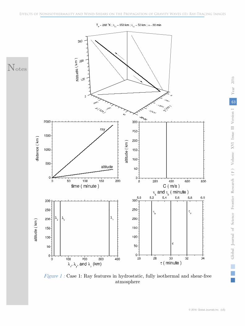
Figure 1 :
Case 1: Ray features in hydrostatic, fully isothermal and shear-free atmosphere
Effects of Nonisothermality and Wind-Shears on the Propagation of Gravity Waves (II): Ray-Tracing Images
1
Globa
lJo
urna
lof
Scienc
eFr
ontie
rResea
rch
V
olum
eXVI
Iss ue
e
rsion
IV
IIIYea
r20
16
63
( F)
Notes
© 2016 Global Journals Inc. (US)
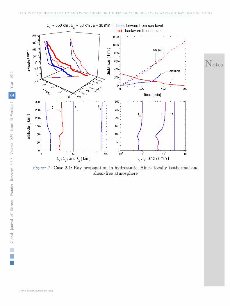
Figure 2 : Case 2-1: Ray propagation in hydrostatic, Hines’ locally isothermal andshear-free atmosphere
64
Globa
lJo
urna
lof
Scienc
eFr
ontie
rResea
rch
V
olum
eYea
r20
16XVI
Iss u
e e
rsion
IV
III( F
)
© 2016 Global Journals Inc. (US)
Effects of Nonisothermality and Wind-Shears on the Propagation of Gravity Waves (II): Ray-Tracing Images
Notes

Figure 3 : Case 2-2: Altitude profiles of _0 and its gradients, as well as p0, in
hydrostatic, Hines’ locally isothermal and shear-free atmosphere
1
Globa
lJo
urna
lof
Scienc
eFr
ontie
rResea
rch
V
olum
eXVI
Iss ue
e
rsion
IV
IIIYea
r20
16
65
( F)
Effects of Nonisothermality and Wind-Shears on the Propagation of Gravity Waves (II): Ray-Tracing Images
Notes
© 2016 Global Journals Inc. (US)

Figure 4 : Case 2-3: Altitude profiles of and its gradients, as well as , in hydrostatic, Hines’ locally isothermal and shear-free atmosphere
Figure 5 : Case 2-4: Altitude profiles of WKB _ in hydrostatic, Hines’ locally isothermaland shear-free atmosphere
66
Globa
lJo
urna
lof
Scienc
eFr
ontie
rResea
rch
V
olum
eYea
r20
16XVI
Iss u
e e
rsion
IV
III( F
)
© 2016 Global Journals Inc. (US)
Effects of Nonisothermality and Wind-Shears on the Propagation of Gravity Waves (II): Ray-Tracing Images
Notes
T0 C
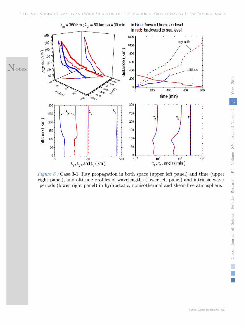
Figure 6 : Case 3-1: Ray propagation in both space (upper left panel) and time (upperright panel), and altitude profiles of wavelengths (lower left panel) and intrinsic waveperiods (lower right panel) in hydrostatic, nonisothermal and shear-free atmosphere.
1
Globa
lJo
urna
lof
Scienc
eFr
ontie
rResea
rch
V
olum
eXVI
Iss ue
e
rsion
IV
IIIYea
r20
16
67
( F)
Effects of Nonisothermality and Wind-Shears on the Propagation of Gravity Waves (II): Ray-Tracing Images
Notes
© 2016 Global Journals Inc. (US)

Figure 7 : Case 3-2: Altitude profiles of mean-field temperature (upper left panel) andits gradients in x (upper right panel), y (lower left panel), and z (lower right panel) in
hydrostatic, nonisothermal and shear-free atmosphere
68
Globa
lJo
urna
lof
Scienc
eFr
ontie
rResea
rch
V
olum
eYea
r20
16XVI
Iss u
e e
rsion
IV
III( F
)
© 2016 Global Journals Inc. (US)
Effects of Nonisothermality and Wind-Shears on the Propagation of Gravity Waves (II): Ray-Tracing Images
Notes
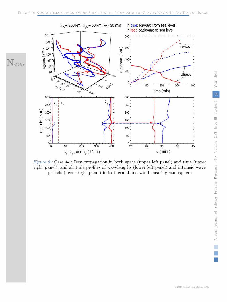
Figure 8 : Case 4-1: Ray propagation in both space (upper left panel) and time (upperright panel), and altitude profiles of wavelengths (lower left panel) and intrinsic wave
periods (lower right panel) in isothermal and wind-shearing atmosphere
1
Globa
lJo
urna
lof
Scienc
eFr
ontie
rResea
rch
V
olum
eXVI
Iss ue
e
rsion
IV
IIIYea
r20
16
69
( F)
Effects of Nonisothermality and Wind-Shears on the Propagation of Gravity Waves (II): Ray-Tracing Images
Notes
© 2016 Global Journals Inc. (US)

Figure 9 : Case 4-2: Altitude profiles along ray paths of WKB _ (upper panel), andmean-field wind (lower left panel: zonal direction; lower right panel: meridional
direction) in isothermal and wind-shearing atmosphere
70
Globa
lJo
urna
lof
Scienc
eFr
ontie
rResea
rch
V
olum
eYea
r20
16XVI
Iss u
e e
rsion
IV
III( F
)
© 2016 Global Journals Inc. (US)
Effects of Nonisothermality and Wind-Shears on the Propagation of Gravity Waves (II): Ray-Tracing Images
Notes
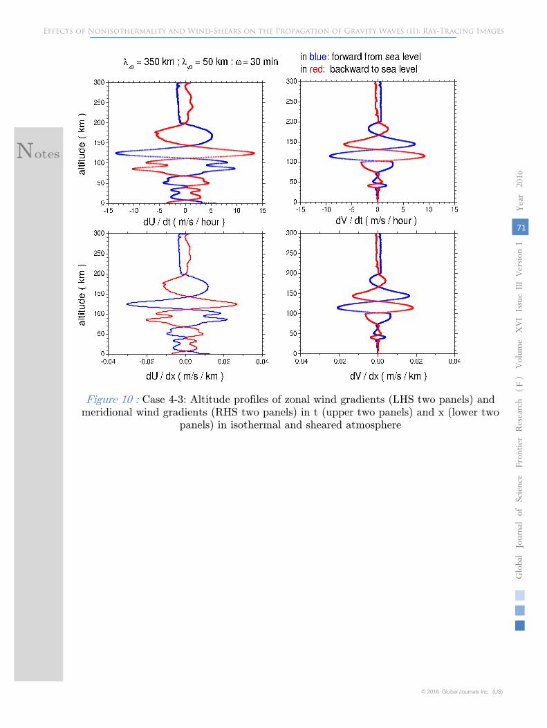
Figure 10 : Case 4-3: Altitude profiles of zonal wind gradients (LHS two panels) andmeridional wind gradients (RHS two panels) in t (upper two panels) and x (lower two
panels) in isothermal and sheared atmosphere
1
Globa
lJo
urna
lof
Scienc
eFr
ontie
rResea
rch
V
olum
eXVI
Iss ue
e
rsion
IV
IIIYea
r20
16
71
( F)
Effects of Nonisothermality and Wind-Shears on the Propagation of Gravity Waves (II): Ray-Tracing Images
Notes
© 2016 Global Journals Inc. (US)

Figure 11 : Case 4-4: Altitude profiles of zonal wind gradients (LHS two panels) andmeridional wind gradients (RHS two panels) in y (upper two panels) and z (lower two
panels) in isothermal and sheared atmosphere
72
Globa
lJo
urna
lof
Scienc
eFr
ontie
rResea
rch
V
olum
eYea
r20
16XVI
Iss u
e e
rsion
IV
III( F
)
© 2016 Global Journals Inc. (US)
Effects of Nonisothermality and Wind-Shears on the Propagation of Gravity Waves (II): Ray-Tracing Images
Notes
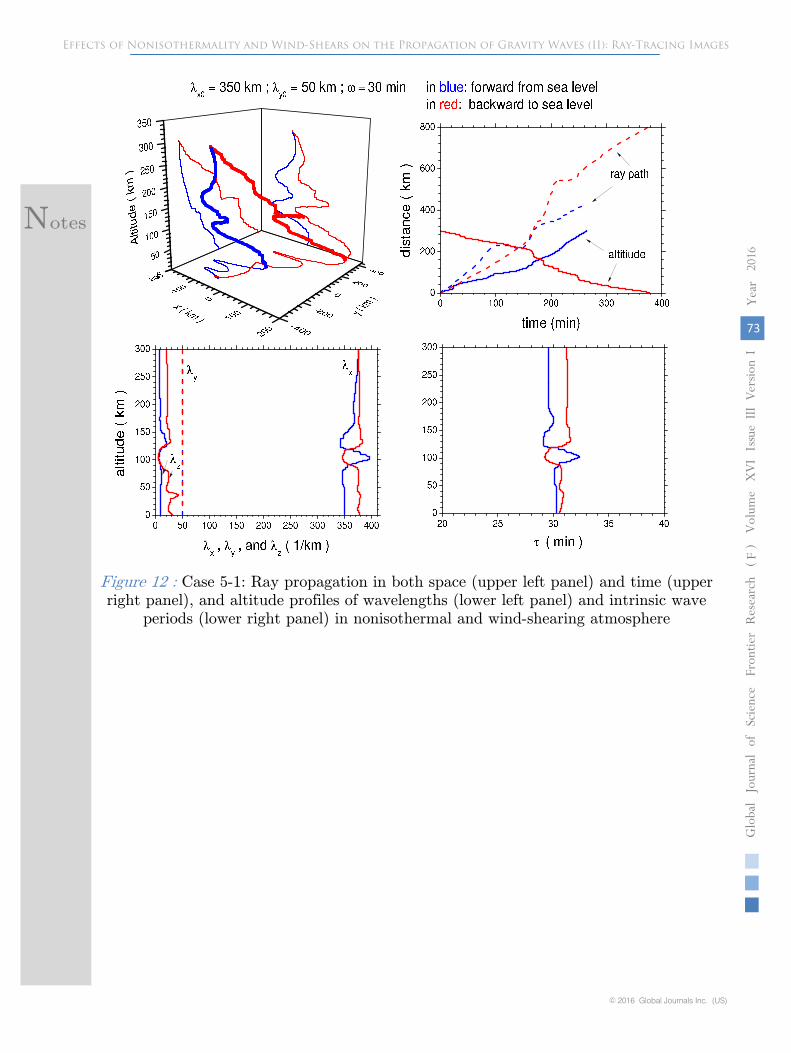
Figure 12 : Case 5-1: Ray propagation in both space (upper left panel) and time (upper right panel), and altitude profiles of wavelengths (lower left panel) and intrinsic wave
periods (lower right panel) in nonisothermal and wind-shearing atmosphere
1
Globa
lJo
urna
lof
Scienc
eFr
ontie
rResea
rch
V
olum
eXVI
Iss ue
e
rsion
IV
IIIYea
r20
16
73
( F)
Effects of Nonisothermality and Wind-Shears on the Propagation of Gravity Waves (II): Ray-Tracing Images
Notes
© 2016 Global Journals Inc. (US)
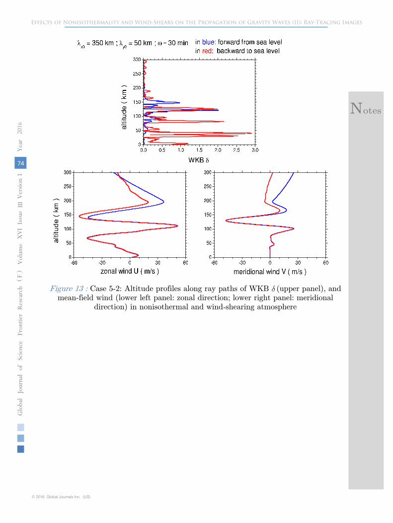
Figure 13 : Case 5-2: Altitude profiles along ray paths of WKB (upper panel), andmean-field wind (lower left panel: zonal direction; lower right panel: meridional
direction) in nonisothermal and wind shearing atmosphere
δ
-
74
Globa
lJo
urna
lof
Scienc
eFr
ontie
rResea
rch
V
olum
eYea
r20
16XVI
Iss u
e e
rsion
IV
III( F
)
© 2016 Global Journals Inc. (US)
Effects of Nonisothermality and Wind-Shears on the Propagation of Gravity Waves (II): Ray-Tracing Images
Notes
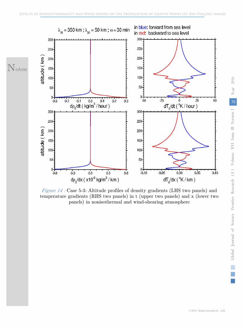
Effects of Nonisothermality and Wind-Shears on the Propagation of Gravity Waves (II): Ray-Tracing Images
Figure 14 : Case 5-3: Altitude profiles of density gradients (LHS two panels) andtemperature gradients (RHS two panels) in t (upper two panels) and x (lower two
panels) in nonisothermal and wind-shearing atmosphere
1
Globa
lJo
urna
lof
Scienc
eFr
ontie
rResea
rch
V
olum
eXVI
Iss ue
e
rsion
IV
IIIYea
r20
16
75
( F)
Notes
© 2016 Global Journals Inc. (US)
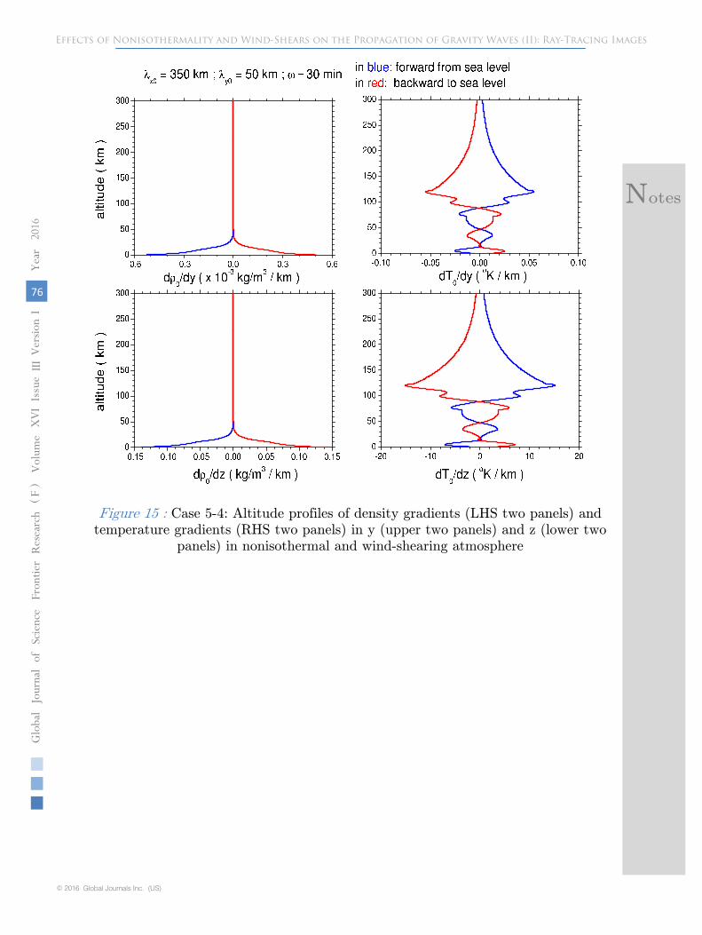
Figure 15 : Case 5-4: Altitude profiles of density gradients (LHS two panels) andtemperature gradients (RHS two panels) in y (upper two panels) and z (lower two
panels) in nonisothermal and wind-shearing atmosphere
76
Globa
lJo
urna
lof
Scienc
eFr
ontie
rResea
rch
V
olum
eYea
r20
16XVI
Iss u
e e
rsion
IV
III( F
)
© 2016 Global Journals Inc. (US)
Effects of Nonisothermality and Wind-Shears on the Propagation of Gravity Waves (II): Ray-Tracing Images
Notes

Figure 16 : Case 5-5: Altitude profiles of zonal wind gradients (LHS two panels) andmeridional wind gradients (RHS two panels) in t (upper two panels) and x (lower two
panels) in nonisothermal and wind-shearing atmosphere
1
Globa
lJo
urna
lof
Scienc
eFr
ontie
rResea
rch
V
olum
eXVI
Iss ue
e
rsion
IV
IIIYea
r20
16
77
( F)
Effects of Nonisothermality and Wind-Shears on the Propagation of Gravity Waves (II): Ray-Tracing Images
Notes
© 2016 Global Journals Inc. (US)
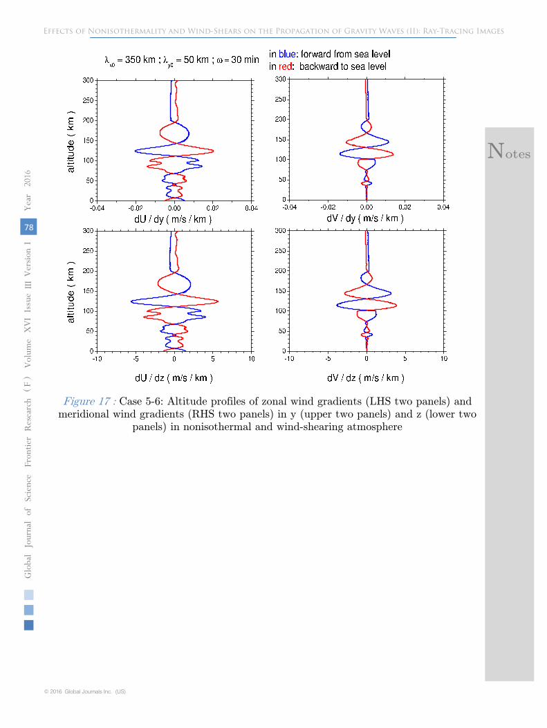
Figure 17 : Case 5-6: Altitude profiles of zonal wind gradients (LHS two panels) andmeridional wind gradients (RHS two panels) in y (upper two panels) and z (lower two
panels) in nonisothermal and wind-shearing atmosphere
78
Globa
lJo
urna
lof
Scienc
eFr
ontie
rResea
rch
V
olum
eYea
r20
16XVI
Iss u
e e
rsion
IV
III( F
)
© 2016 Global Journals Inc. (US)
Effects of Nonisothermality and Wind-Shears on the Propagation of Gravity Waves (II): Ray-Tracing Images
Notes

Figure 18 : Case 6-1: Propagating ray paths in space in nonisothermal and windshearingatmosphere under different initial wavelengths
Effects of Nonisothermality and Wind-Shears on the Propagation of Gravity Waves (II): Ray-Tracing Images
1
Globa
lJo
urna
lof
Scienc
eFr
ontie
rResea
rch
V
olum
eXVI
Iss ue
e
rsion
IV
IIIYea
r20
16
79
( F)
Notes
© 2016 Global Journals Inc. (US)

Figure 19 : Case 6-2: the same as Fig.18 but ray paths and vertical increments in time
80
Globa
lJo
urna
lof
Scienc
eFr
ontie
rResea
rch
V
olum
eYea
r20
16XVI
Iss u
e e
rsion
IV
III( F
)
© 2016 Global Journals Inc. (US)
Effects of Nonisothermality and Wind-Shears on the Propagation of Gravity Waves (II): Ray-Tracing Images
Notes

Figure 20 : Case 6-3: Development of and versus ray path in wave propagation
1
Globa
lJo
urna
lof
Scienc
eFr
ontie
rResea
rch
V
olum
eXVI
Iss ue
e
rsion
IV
IIIYea
r20
16
81
( F)
Effects of Nonisothermality and Wind-Shears on the Propagation of Gravity Waves (II): Ray-Tracing Images
λx,y,z τ
Notes
© 2016 Global Journals Inc. (US)