Effects of non-tracking solar collectororientation on energy production:

Photovoltaic systems

Tauno Toikka

Master’s thesisUniversity of Jyvaskyla, Department of PhysicsMaster’s Degree Program in Renewable Energy

29.02.2012Instructor: Jussi Maunuksela

Contact: tauno.toikka@solaropt.com

Preface

This study has been carried out in Master’s Degree Programme in Re-newable Energy at the University of Jyvaskyla.

I would like to thank my supervisor Jussi Maunuksela, Ph.D. who gaveme free hands to make my thesis in the way I felt it had to be done andstill advised and helped me whenever there was a need. I am grateful to mygirlfriend Iida Korenius who was supportive and helpful through the wholestudy process. I would also like to thank my friend physics student JanneKauppinen of all the reasonable and constructive criticism.

Jyvaskyla, January 2012Tauno Toikka

1

Abstract

This Master’s thesis proposes a new method for calculating theoptimum tilt and orientation angle of a fitted solar collector. In ad-dition to using geographical data, this method takes into account theradiation data and weather statistics of prospective locations. Thismakes the calculations valid not only for certain latitudes, but alsofor certain radiation and weather conditions.

Calculations were done by estimating the energy production of agiven solar array using a sequence of different tilt angles and orienta-tion angles. Special attention was given to shaded solar arrays and ar-rays made up of photovoltaic modules. Specific radiation and weatherdata was used for both locations. Also, the different attributes ofdifferent phovoltaic modules were taken into consideration.

The proposed method is illustrated with two examples. Two solararrays in two different locations were chosen: one in Southern Finlandin Helsinki (60.12o N, 24.57o E), and the other in Central Finland inViitasaari (63.07o N, 25.68o E).

The calculations for the solar array in Helsinki, which is in plan-ning stage, take into account the shading caused by row installation.Calculations were made for c-Si PV modules. The optimum tilt an-gle was calculated as 28.6o and the optimum orientation as 0.1o fromsouth to west.

The array in Viitasaari is an existing one, and the calculated op-timum tilt and orientation angles were compared to the actual an-gles used at the location. The solar collector used there is a semi-transparent a-Si PV module. The optimum tilt angle was calculatedas 46.4o, and the actual angle at the site was 5o. The optimum orien-tation angle was calculated as 4.3o from south to east, and angle usedwas 0o, i.e. south.

2

Contents

1 Introduction 5

2 Definitions 92.1 Direct and diffuse sun light . . . . . . . . . . . . . . . . . . . . 92.2 Solar constant . . . . . . . . . . . . . . . . . . . . . . . . . . . 92.3 Declination . . . . . . . . . . . . . . . . . . . . . . . . . . . . 92.4 Hour angle . . . . . . . . . . . . . . . . . . . . . . . . . . . . . 92.5 Zenith and profile angle from the position of the sun . . . . . 112.6 Air Mass . . . . . . . . . . . . . . . . . . . . . . . . . . . . . . 122.7 Ground reflectance . . . . . . . . . . . . . . . . . . . . . . . . 13

3 Radiation on horizontal surface 153.1 Extraterrestrial radiation on a horizontal surface . . . . . . . . 153.2 Clearness index . . . . . . . . . . . . . . . . . . . . . . . . . . 15

4 Radiation on tilted surface 174.1 Ratio between beam radiation on horizontal surface to beam

radiation on tilted surface . . . . . . . . . . . . . . . . . . . . 174.2 Radiation components . . . . . . . . . . . . . . . . . . . . . . 184.3 Isotropic sky . . . . . . . . . . . . . . . . . . . . . . . . . . . . 194.4 Anisotropic sky . . . . . . . . . . . . . . . . . . . . . . . . . . 19

4.4.1 Perez model . . . . . . . . . . . . . . . . . . . . . . . . 19

5 Self shading 235.1 Beam radiation component . . . . . . . . . . . . . . . . . . . . 255.2 Isotropic diffuse radiation component . . . . . . . . . . . . . . 285.3 Circumsolar diffuse radiation component . . . . . . . . . . . . 285.4 Horizontal diffuse radiation component . . . . . . . . . . . . . 295.5 Ground reflected radiation component . . . . . . . . . . . . . 295.6 Total radiation on tilted surface under shading effect . . . . . 30

6 Effect of glass cover and dust 31

7 Photovoltaic generation 347.1 One diode equivalent circuit model . . . . . . . . . . . . . . . 347.2 Short circuit current ISC under real operation conditions . . . 377.3 Open circuit voltage under real operation conditions . . . . . . 397.4 Cell temperature . . . . . . . . . . . . . . . . . . . . . . . . . 41

7.4.1 Using NOCT . . . . . . . . . . . . . . . . . . . . . . . 417.4.2 Using wind speed . . . . . . . . . . . . . . . . . . . . . 41

3

7.5 Power generated . . . . . . . . . . . . . . . . . . . . . . . . . . 42

8 Results 448.1 Case Pitajanmaki . . . . . . . . . . . . . . . . . . . . . . . . . 44

8.1.1 Example calculation: radiation on tilted surface . . . . 448.1.2 Example calculation: effect of shading, glass cover and

dust . . . . . . . . . . . . . . . . . . . . . . . . . . . . 468.1.3 Example calculation: photovoltaic generation . . . . . 508.1.4 Final result: tilt and orientation angle effect on yield . 52

8.2 Case Viitasaari . . . . . . . . . . . . . . . . . . . . . . . . . . 53

9 Discussion 59

10 Conclusions 65

4

1 Introduction

The need to investigate the issue of this thesis arose in another context. Whenmaking my Research exercise the answer about optimal tilt angle for fittedsolar collector was needed. I personally found it hard to find the preciseinformation about what is the optimal orientation and above all, what isthe optimal tilt angle for fitted solar collectors from leading literatures andfrom scientific articles. If the answer was found about orientation then thetypical answer was south, which is pretty reasonable. On the other handthe typical answer about tilt angle was in the form of Latitude ± 10o orLatitude− 20o to Latitude. The most sophisticated answer was found fromLuque [4]. In this reference the suggestion was a first degree function withone parameter, which was Latitude. In all suggestions the optimal tilt angledepended on only one parameter, which was Latitude.

It is obvious that latitude is not the only parameter that has effect on theoptimum tilt angle. For example London (England) and Kiev (Ukraine) arepretty much in same latitude. London is a foggy place, and Kiev is a sunnyplace. Thus, in Kiev the greater percentage of radiation comes directly fromthe sun compared to London. As this was the case, collectors in Kiev shouldbe oriented more towards to the sun compared to London. On the otherhand, in London collectors should be directed more towards the sky dome.Thus, the optimum tilt angle for collectors in Kiev might be near latitudebut in London the angle might be latitude minus some degrees.

In our modern world where everything needs to be optimized particularlyin the sector of energy production, we might ask why the direction of solarcollectors does not need to be optimized. Solid state physicists are doinga considerable amount of work to make our solar modules more and moreeffective, yet we place them on our roofs in more or less random directions.

In some sense it is understandable. Module makers need to sell modulesand thus it is in their best interests to make them as good as possible. Themiddle man between module makers and consumers intends to sell modules,and this he will do with the module specifications. The final yield is not hismain concern. When a module has been sold it is the clients task to optimizeit. Typically, customers have no ability to estimate the optimum installationfor their solar system. They rely on the seller’s or the manufacturer’s roughapproximations, and in the end pay the price.

It is obvious that installing systems in the optimal direction does notrequire any more physical effort that installing it in some other direction.The only thing needed is adequate estimation and that is the focus of thisthesis.

5

Case Helsinki Pitajanmaki In this case, the sales manager from Sun-Wind Gylling Oy contacted us. For a competitive bidding they needed ten-tative calculations about the optimum tilt angle and energy yield for a PV-power plant. The planned system is in the size scale of 140 kWp (biggest inScandinavia) and it is planned to be located in Pitajanmaki, Helsinki. Thesolar array is planned to contain 700 Swedmodule GPV200 solar modules[Appendix 2]. Preliminary requirements were 50 rows of modules with 14modules in each row. The distance between the rows had a requirement of3 m and an orientation of 20o from south to west. The whole system is tobe placed on rooftop supported by stands.

Near Pitajanmaki lies Kumpula, where Finnish Meteorological Institute(FMI) [14] happens to have measurement station for solar radiation. Thedistance between these two locations is only between 4 to 5 km. For our cal-culations we assume radiation and weather conditions to be equal in Kumpulaand Pitajanmaki.

One year measurement data was received from FMI measured in HelsinkiKumpula for tentative calculations for Sunwind Gylling Oy. The three yearsmeasurement data was received later for the use of this thesis, because themeasurement station has existed only for a while. Only round years wereused as data because it is not reasonable to stress any particular season. Thedata for tentative calculations besides date and time included global anddiffuse radiation for each hours of the year 2009. The Data from FMI usedhere also includes average ambient temperature and average wind speed foreach hour during the years 2007-2009.

In addition to this, the data on the location of the solar system wasnecessary. The data on location can be found in table 1. Also, the necessarydata on planned solar modules can be found in table 2.

Table 1: Essential data from Helsinki Kumpula (Radiation measurementstation). Data is from [14].

Local Latitude (φ) 60.12o

Local Longitude (LL) 24.57o

Average starting time of thermal winter 26.12Average ending time of thermal winter 30.03

Case Viitasaari Viitasaari is a small town in central Finland and whichhas a service station. The cafeteria of the service station has a terrace roofmade of transparent PV-modules (fig. 1) [Appendix 3]. The size of thesolar system is 4.2 kWp with a total of 154 ASITHRU-30-SG modules. The

6

Table 2: Essential data about solar modules planned to use in HelsinkiPitajanmaki. All data are from manufacturer’s data [Appendix 2]. SubscriptSTC stands for standard test conditions: 1000 W/m2, 25oC, 1.5 AM .

VOC,STC 36.6 VVMPP,STC 29.0 VISC,STC 7.58 AIMPP,STC 7.01 ANOCT 46oCTemperature coefficient for voltage −0.0034/KTemperature coefficient for current 0.00034/KCell type c-SiBack surface of the module TedlarNumber of cells in module 60

tilt and orientation angles are 5o and 0o which are not optimums, but aredefined by architectural points of departures. Our interest here is to discoverthe optimum tilt and orientation angles, and estimate how much has beenlost with existing settings.

Figure 1: The terrace roof of the service station in Viitasaari [13].

University of Jyvaskyla has a weather station in Viitasaari. The globalradiation data, the ambient temperature data and the wind speed data havebeen collected during the years 2004-2009. Also, the energy yield of the solararray has been filed. In our calculations the data of the years 2004 and 2009have been excluded because there is no data from complete years. Also,

7

the year 2005 has been excluded due to some confusion with time filing inthe beginning of the year. Calculations were done using date, time, globalradiation, average ambient temperature and average wind speed for eachhour during the years 2006-2008. Also the information in tables 3 and 4 wereused.

Table 3: Essential data about location of ViitasaariLocal Latitude (φ) 63.07o

Local Longitude (LL) 25.86o

Average starting time of thermal winter [14] 26.11Average ending time of thermal winter [14] 20.04

Table 4: Essential data about solar modules used in Viitasaari [Appendix3]. Subscript STC stands for standard test conditions: 1000 W/m2, 25oC,1.5 AM .

VOC,STC 49 VVMPP,STC 36 VISC,STC 1.02 AIMPP,STC 0.75 ANOCT -Temperature coefficient for voltage −0.0033/KTemperature coefficient for current 0.0008/KCell type a-SiBack surface of the module GlassNumber of cells in module -

The underlying pattern in this thesis is to calculate the radiation on atilted surface as accurately as possible, to take into account the shading effectin a reasonable way and to do photovoltaic calculations using only the datathat is typically available in the manufacture’s data sheets. In the field ofradiation we use the symbols from Ref. [3], in the field of shading effect weuse symbols from Ref. [6] and in the field of photovoltaic generation we usesymbols from Ref. [4]. List of the basic symbols used in this work can befound in Nomenclature in [Appendix 1].

Words radiation and irradiation here were not used randomly: radiationimplies the amount of solar radiation in joules per square meter J/m2 andirradiation implies to the power of illumination produced by radiation persquare meter W/m2. Illumination is our general way to express that radiationor irradiation occurs.

8

2 Definitions

2.1 Direct and diffuse sun light

Direct sunlight represents a beam which has not suffered scattering in theearth’s atmosphere. Diffused sunlight has suffered scattering in the earth’satmosphere. Scattering can be caused by air, dust, aerosol, clouds, drops ofwater or ground (and all the obstacles the ground includes).

In this thesis we denote solar radiation as H. With the subscript b wedenote direct solar radiation (Hb). With the subscript d we denote diffusedsolar radiation (Hd). Hb and Hd have been quantified the way that Hd+Hb =Hg, where Hg is global radiation [2].

2.2 Solar constant

Solar constant gives the average sun irradiation outside the earths atmo-sphere. In this thesis we use symbol Gsc for it. There are some variationsin this constant in different literatures. For example in Duffie & Becham [3]Gsc is 1367 W/m2 and in Meinel [2] Gsc is 1353 W/m2. In this work we useGsc = 1367 W/m2.

2.3 Declination

If we assume that the earths orbit forms a plane around the sun and theEarths rotation forms a rotation axis, then the angle between the axis andthe plane varies from −23.45o to 23.45o during a year (see fig. 2). Thisvariation angle is called declination and is denoted as δ. Declination can becalculated from the following equation [1]:

δ = 23.45o sin

(360o 284 + n

365

)(1)

where n is the number of a day of a year. For example for the eight day ofFebruary n=39 and δ = −15.52o.

2.4 Hour angle

The symbol ω is used for an hour angle. Hour angle describes earths rotationaround its own axis. In one day the hour angle goes from −180o to 180o.For solar noon (=sun is in it’s uppermost position) the hour angle has beenchosen to be 0o. In every one hour after the noon the hour angle increases 15degrees and in every one hour before noon hour angle decreases 15 degrees.

9

Figure 2: Earth’s movement on its orbit plane that causes the declination[4].

That means for example that at 12:00 ω = 0o, at 13:00 ω = 15o, at 14:00ω = 30o, at 11:00 ω = −15o, at 10:00 ω = −30o and so on [1].

Solar time Solar time describes the dependence between the angular mo-tion of the sun across the sky, the time we use and the location of the observer.It can expressed as

solar time = 15o ∗ (TO − AO − 12) + (LL− LH) (2)

where LL is the local longitude and LH is the longitude of the local timezone,both of them in degrees [4](positive for east longitudes and negative for westlongitudes). TO is the local official time and AO is the correction parameter,both in hours. Correction parameter is needed for example when clocks areset ahead by one hour in summer time. In that case AO = 1.

Equation of time There is a small variation in earth rotation that hasnot been included in the time that humans use. The variation is annual andit is in scale of ±4o (∼ ±15 min). The variation is illustrated in figure 3.

Equation of time describes the variation and it can be expressed as

E =1

4229.2o(0.000075 + 0.001868 cosB − 0.032077 sinB

− 0.014615 cos(2B)− 0.04089 sin(2B))(3)

where B = (n− 1)360o

365and n is the number of a day of a year [3]. Thus the

hour angle that conforms its definition is

ω = solar time+ E (4)

10

Figure 3: Variation in hour angle compared to solar time.

2.5 Zenith and profile angle from the position of thesun

In figure 4 there is illustrated horizontal surface and tilted surface. Theangle that tilted surface is tilted compared to horizontal surface is β. Theorientation of tilted surface is γ and it is zero in south, positive from south towest and negative from south to east. Zenith is the normal of the horizontalsurface. The angle between the direction of beam radiation and zenith iscalled zenith angle θz and the angle between the direction of beam radiationand horizontal surface is called solar altitude angle αs.

The angle of incidence is the angle between the direction of beam radiationand the normal of tilted surface. It is denoted as θ. The angle of incidenceis related to tilt and orientation angle in a way that can be described withequation

cos θ = sin δ sinφ cos β − sin δ cosφ sin β cos γ + cos δ cosφ cos β cosω

+ cos δ sinφ sin β cos γ cosω + cos δ sin β sin γ sinω(5)

where ω is the hour angle, δ is the declination and φ is the local latitude [3].For horizontal surfaces β = 0. That means that for horizontal surfaces

from equation 5 only first and third terms remains. Thus we get relationbetween zenith angle for horizontal surface with other angles as:

cos θz = cosφ cos δ cosω + sinφ sin δ (6)

11

Figure 4: Horizontal surface, tilted surface, the sun, zenith angle as θz, sur-face tilt angle as β, surface slope/orientation angle as γ and solar altitudeangle as αs [3].

In figure 5 there is illustrated profile angle αp which is also an essentialangle. Other angles in figure 5 are the same as in the figure 4. Profile angleis related to other angles of figures 4 and 5 in the following way:

tanαp =tanαs

cos(γs − γ)(7)

where γs is the solar azimuth angle and in equation form

γs = sign(ω)

∣∣∣∣ cos−1

(cos θz sinφ− sin δ

sin θz cosφ

)∣∣∣∣ (8)

and αs solar altitude angle and as figure 4 demonstrates αs = 90o − θz.

2.6 Air Mass

Air mass AM is the unitless measure of the relative path length of solarradiation through the atmosphere. It has been defined to be one when solar

12

Figure 5: Profile angle αp and some other essential angles related to tiltedsurface R and the suns position [3].

radiation goes vertically through the atmosphere at sea level. That meansthat AM = 1 when sun is at zenith. AM increases when the solar zenithangle increases. An approximative expression for air mass is as follows [3]:

AM =1

cos θz

(9)

According to this equation AM goes infinite when θz → 90o. This is anunphysical situation and we can expect that equation 9 gives inaccuratevalues when the sun is near the horizon. On the other hand irradiation levelsat these moments are low. Thus also the effect of inaccurate AM is low whencalculating overall radiation.

2.7 Ground reflectance

Ground reflects light and when solar collector is tilted some of that light willend on solar collector. Ground reflectance can be quantified as the relativeamount of light that ground reflects.

Ground reflectance is denoted as ρ. It is a fraction between reflectedradiation to total radiation. Thus it is ranged between 0 and 1 in the waythat 0 means no reflected radiation at all and 1 means that all radiationreflects.

If there is no information available about the magnitude of ground re-flectance, using ρ = 0.2 for approximation is recommended [2], [3]. It is agood approximation for most cases, but significant variation in the ground

13

reflectance exists when the ground is cowered with snow. A good averageestimation for snow covered ground is ρ = 0.7 [2], [3].

14

3 Radiation on horizontal surface

3.1 Extraterrestrial radiation on a horizontal surface

The average extraterrestrial irradiation is defined by solar constant which is1367 W/m2. However, it varies during a year because of the variation of thedistance between the earth and the sun. The variation of the extraterrestrialirradiation is about ±3% during a year [2].

Extraterrestrial irradiation can be expressed as a function of a day of ayear with the following equation [3]

Gon = Gsc

(1 + 0.033 cos

360on

365

)(10)

where Gsc is solar constant and n is the number of a day of a year.For horizontal surface equation 10 is

Go = Gsc

(1 + 0.033 cos

360on

365

)cos θz (11)

This can be considered as irradiation on earth’s surface without the atmo-sphere. Using equation 6 in equation 11 we get

Go = Gsc

(1 + 0.033 cos

360n

365

)(cosφ cos δ cosω + sinφ sin δ) (12)

In some cases we need to know extraterrestrial radiation on horizontalsurface at certain period of time in a day. An equation for those cases canbe achieved by integrating the equation 12 over ω. Integration gives us

H0 =12 ∗ 3600

πGsc

(1 + 0.033 cos

360on

365

)[cosφ cos δ(sinω2 − sinω1)

+π(ω2 − ω1)

180sinφ sin δ

] (13)

where ω1 and ω2 are limits of time in form of hour angles so that ω1 < ω2

[3]. This equation gives the extraterrestrial radiation on horizontal surfacebetween times ω1 and ω2.

3.2 Clearness index

In general there are two types of radiation data available. In most cases thedata of solar radiation is in the form of global radiation. Global radiation

15

means total radiation on a horizontal surface. Some solar radiation measure-ment stations can give global and diffuse radiation components separately.When there is only global radiation data available estimation of diffuse radi-ation component needs to be done. A key for estimating the diffuse radiationis so called clearness index. Clearness index has been defined as

kT =Hg

H0

(14)

where Hg is total radiation on horizontal surface and Ho is extraterrestrialradiation [3].

Correlation between clearness index kT and Hd/Hg has been found inhourly repeated measurements. Figure 6 illustrates the type of data that hasbeen measured. This type of data has been received from many studies. The

Figure 6: Measured correlation between clearness index and diffuse radiationdivided by total radiation [3].

curve fittings from three different studies are shown in figure 7.In this thesis we use the curve fitting by Erbs et al. [10] from figure 7.

The analytical expression for this curve is

Hd

Hg

=

1.0− 0.09kT for kT 6 0.220.9511− 0.1604kT + 4.388k2

T

−16.0638k3T + 12.366k4

T for 0.22 < kT 6 0.800.165 for kT > 0.80

(15)

16

Figure 7: Curve fitting from three different measurements illustrating thecorrelation between kT and Hd/Hg [3].

4 Radiation on tilted surface

Typical type of radiation data available is the data of radiation on horizontalsurface. On the other hand, horizontal plane is not the plane where highestannual radiation occurs (equator is an exception). Thus, we need to find amethod to estimate the radiation on tilted surface based on the radiationdata on horizontal surface. The following sections will present some of thesemethods.

4.1 Ratio between beam radiation on horizontal sur-face to beam radiation on tilted surface

When transformation from radiation on horizontal surface to radiation ontilted surface needs to be done, we need ratio between beam radiation ontilted surface to beam radiation on horizontal surface. This ratio is denotedin this thesis as Rb:

Rb =Beam radiation on tilted surface

Beam radiation on horizontal surface(16)

Using equations 5 and 6 it can be written as

Rb =Hb ∗ cos θ

Hb ∗ cos θz

(17)

where Hb is a direct beam radiation [3]. Thus

Rb =cos θ

cos θz

. (18)

17

The term cos θ gives negative values when radiation incidences on backsurface of solar collector. When we assume that radiation on back surface isnot exploitable then

Rb =min(0, cos θ)

cos θz

(19)

In equation 19 there is cos θz in denominator. The term cos θz −→ 0 whenθz −→ 90o. This happens when the sun is rising or setting down. In thesecases Rb can have unrealistically high values because of the low denominatorin equation 19. In hourly calculations for those hours, during which the sunis rising or setting down, reference [3] suggests to use equation:

Rb.ave =

∫ ωii

ωicos θ dω∫ ωii

ωicos θz dω

=A

B(20)

where

A = (sin δ sinφ cos β − sin δ cosφ sin β cos γ)π

180(ωii − ωi)

+ (cos δ cosφ cos β + cos δ sinφ sin β cos γ)(sinωii − sinωi)

− (cos δ sin β sin γ)(cosωii − cosωi)

(21)

andB = (cosφ cos δ)(sinωii − sinωi) + (sinφ sin δ)

π

180(ωii − ωi) (22)

In noon ωi is the hour angle of the starting point of the hour under exam-ination and ωii is the sunset hour angle. In morning ωi is the sunrise hourangle, that is -(sunset hour angle), and ωii is the ending point of the hourunder examination. Sunset hour angle ωs can be found from equation:

cosωs = − tanφ tan δ (23)

4.2 Radiation components

To make radiation calculations on tilted surface possible we need to splittotal radiation into components. Beam and diffuse radiation occur on tiltedsurface. Theoretically, light reflected from ground does not end up on hor-izontal surface but it does end up on tilted surface. Thus, general way toexpress radiation on tilted surface in three components is

HT = HT,b +HT,d +HT,r (24)

where HT,r is radiation reflected from ground [4].

18

4.3 Isotropic sky

Isotropic sky assumption is a simple way to calculate all three radiationcomponents (HT,b, HT,d, HT,r) on tilted surface. The main idea of it is thatit assumes diffuse radiation coming equally from all directions of skydome[3]. For tilted surface the relative visible part of the skydome to the surfacecan be expressed as (1 + cos β)/2 where β is tilt angle of the surface.

Also, ground reflection is assumed to be homogeneous from all directions.It means that the amount of irradiation you receive is constant regardless ofthe direction you look at the ground.

The relative visible part of ground for a tilted surface can be expressedas (1− cos β)/2. Thus equation 24 becomes for isotropic sky as

HT = HbRb +Hd

(1 + cos β

2

)+Hgρ

(1− cos β

2

)(25)

4.4 Anisotropic sky

In isotropic sky assumption we assumed diffuse radiation coming equally fromall directions of the skydome. It is a good approximation, but true only forheavily overcast skies. Figure 8 illustrates diffuse radiation distribution overskydome in a real case. In figure 8 the isotropic sky case would be a straighthorizontal line representing diffuse radiation distribution. From figure 8 itcan be found that the highest diffuse radiation occurs from skydome nearto the sun. It can be easily seen by eye when examining the sky. Also, thediffuse radiation near the horizon can be higher than elsewhere. This showsas a small mound at 80o zenith angle in figure 8.

In anisotropic sky assumption we examine the diffuse radiations in com-ponents. We assume there to be three types of diffuse radiation: isotropicdiffuse which comes from equally all directions of skydome, circumsolar dif-fuse which comes from small area around the sun and diffuse from the hori-zon. Also, beam radiation and ground reflected radiation are included in.The components are illustrated in figure 9.

4.4.1 Perez model

There are few ways to estimate anisotropic sky. Some of them are presentedin [3] and [4]. References [3], [4] and [6] suggest that the best of them is theso-called Perez model [8]. Perez model is the most accurate in taking accountthe different sky conditions. On the other hand, it is also the most complexone.

19

Figure 8: Distribution of diffuse radiation with different zenith angles [3].

Different sky conditions are defined through clearness ε so that

ε =

Hd +Hd ∗ sin−1 β

Hd

+ 5.535 ∗ 10−6θ3z

1 + 5.535 ∗ 10−6θ3z

(26)

where Hd is a diffuse radiation to the horizontal surface, θz is a zenith angleand β is a tilt angle.

Using clearness ε we can calculate circumsolar brightening coefficient F1

and horizontal brightening coefficient F2 so that

F1 = max

[0, f11 + f12∆ +

πθz

180f13

](27)

and

F2 = f21 + f22∆ +πθz

180f23 (28)

Empirically adjusted parameters f11, f12, f13, f21, f22 and f23 are functionsof ε and they can be found in table 5.

Also, other versions of table 5 exist. For example, reference [3] usesclearness table from 1988. The table used in this thesis is from 1990 and wasthe latest to be found and for that reason was chosen to be used here. Thefact that Quaschning [6] presented this table encouraged to use this version.

20

Figure 9: Radiation components in anisotropic sky assumption [3].

Table 5: Parameters for calculating brightening coefficients [8].

ε class range of ε f11 f12 f13 f21 f22 f23

1 1.000 - 1.065 -0.008 0.588 -0.062 -0.060 0.072 -0.0222 1.065 - 1.230 0.130 0.683 -0.151 -0.019 0.066 -0.0293 1.230 - 1.500 0.330 0.487 -0.221 0.055 -0.064 -0.0264 1.500 - 1.950 0.568 0.187 -0.295 0.109 -0.152 -0.0145 1.950 - 2.800 0.873 -0.392 -0.362 0.226 -0.462 0.0016 2.800 - 4.500 1.132 -1.237 -0.412 0.288 -0.823 0.0567 4.500 - 6.200 1.060 -1.600 -0.359 0.264 -1.127 0.1318 6.200 - ∞ 0.687 -0.372 0.250 0.156 -1.377 0.251

Parameter ∆ in equations 27 and 28 is the atmospheric brightness whichis defined as

∆ = AMHd

Hon

(29)

where AM is the air mass, Hd is the diffuse radiation and Hon the extrater-restrial normal incidence radiation which can be found from equation 10.

The diffuse radiation component to tilted surface according to Perezmodel can be written as

Hd,T = Hd

[(1− F1)

(1 + cos β

2

)+ F1

a

b+ F2 sin β

](30)

wherea = max[0, cos θ] (31)

21

andb = max[cos 85, cos θz] (32)

Note thata

bis most of the time same as Rb.

Now total radiation on tilted surface according to Perez model is

HT = HbRb +Hd(1− F1)

(1 + cos β

2

)+HdF1

a

b

+HdF2 sin β +Hgρ

(1− cos β

2

) (33)

It is worth to note that the first term in this equation represents directbeam radiation, the second term represents isotropic diffuse, the third termrepresents circumsolar diffuse, the fourth term represents diffuse from horizonand the fifth term represents radiation reflected from ground. To make iteasier to refer the components of the function 33 in future we denote theequation 33 as

HT = HT,b +HT,d,iso +HT,d,cs +HT,d,hz +HT,r (34)

22

5 Self shading

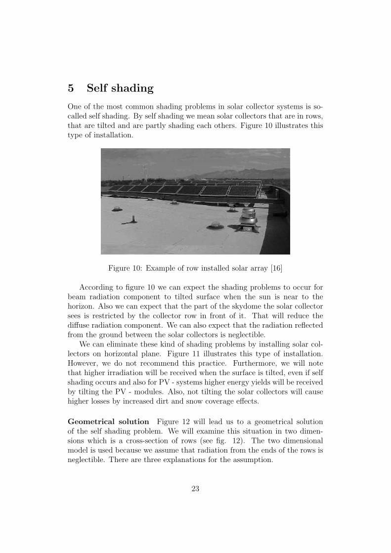
One of the most common shading problems in solar collector systems is so-called self shading. By self shading we mean solar collectors that are in rows,that are tilted and are partly shading each others. Figure 10 illustrates thistype of installation.

Figure 10: Example of row installed solar array [16]

According to figure 10 we can expect the shading problems to occur forbeam radiation component to tilted surface when the sun is near to thehorizon. Also we can expect that the part of the skydome the solar collectorsees is restricted by the collector row in front of it. That will reduce thediffuse radiation component. We can also expect that the radiation reflectedfrom the ground between the solar collectors is neglectible.

We can eliminate these kind of shading problems by installing solar col-lectors on horizontal plane. Figure 11 illustrates this type of installation.However, we do not recommend this practice. Furthermore, we will notethat higher irradiation will be received when the surface is tilted, even if selfshading occurs and also for PV - systems higher energy yields will be receivedby tilting the PV - modules. Also, not tilting the solar collectors will causehigher losses by increased dirt and snow coverage effects.

Geometrical solution Figure 12 will lead us to a geometrical solutionof the self shading problem. We will examine this situation in two dimen-sions which is a cross-section of rows (see fig. 12). The two dimensionalmodel is used because we assume that radiation from the ends of the rows isneglectible. There are three explanations for the assumption.

23

Figure 11: Example of an solar array installed on a horizontal plane.Linkoping’s public library in Sweden [Appendix 2].

Firstly, if solar collectors are properly fitted they are facing south ornear south. This means that direct and circumsolar diffuse end up on solarcollectors when the sun is rising or setting down (see fig. 13). When the sunis setting down it is near the horizon and radiation is going through to thehigh air mass. This leads to low radiation levels during those moments.

Secondly, when radiation is coming from the side of the collector, the angleof incidence θ is high (near to 90o). Increasing angle of incidence causes thedecrease of irradiation.

Third and the most remarkable point is the fact that basically all solarcollectors are covered by glass (PV - systems and solar heat collectors). It isa law of optics that beam of light does not pass the glass at high inclinationangles. Figure 14 gives an example of this.

We can also explain our assumption from another point of view. Whenthe rows are long and the relative distances between the rows are small, wecan assume the rows to be infinitely long. When the rows are infinitely longthen there is no radiation from the ends of the rows. This leads us to asituation where two dimensional examination is acceptable. Now on we callthis assumption as the long row assumption.

In the next chapters we will examine shading effects for all five radiationcomponents from equation 34 separately.

24

Figure 12: Geometrical illustration of angles and dimensions we use here [6].

Figure 13: Illustration of sun position with respect to a properly orientatedsolar array when sun is raising or setting down.

5.1 Beam radiation component

Point P1 on solar collector in figure 12 does not suffer any shading effect. Atthe moment when the sun rises above horizon, point P1 is almost immediatelyilluminated. When sun keeps rising, direct beam radiation starts reachinglower and lower points from solar collector until it reaches to the point of P0.During that period of time the amount of radiation that ends up on solarcollector is about the same as if only the area between P1 and P2 would beunder illumination. In both cases the irradiation is the same. On the otherhand, irradiation is also the same when the whole solar collector is underillumination half of the time of the period.

In case of some solar collectors like solar heat collectors we can use pointP2 as a reference point. That means the whole solar collector is illuminatedby beam radiation when sun rises above angle of α2. The case is equallythe same as when the sun is setting down. Beam radiation stops on solarcollector when the sun has been set down under the angle of α2. Generalizingthis, beam radiation reaches on solar collector when profile angle αp is greater

25

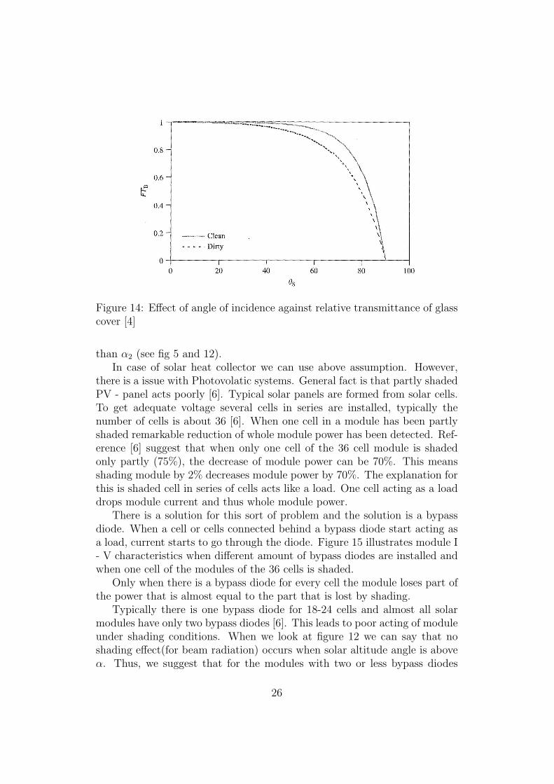
Figure 14: Effect of angle of incidence against relative transmittance of glasscover [4]

than α2 (see fig 5 and 12).In case of solar heat collector we can use above assumption. However,

there is a issue with Photovolatic systems. General fact is that partly shadedPV - panel acts poorly [6]. Typical solar panels are formed from solar cells.To get adequate voltage several cells in series are installed, typically thenumber of cells is about 36 [6]. When one cell in a module has been partlyshaded remarkable reduction of whole module power has been detected. Ref-erence [6] suggest that when only one cell of the 36 cell module is shadedonly partly (75%), the decrease of module power can be 70%. This meansshading module by 2% decreases module power by 70%. The explanation forthis is shaded cell in series of cells acts like a load. One cell acting as a loaddrops module current and thus whole module power.

There is a solution for this sort of problem and the solution is a bypassdiode. When a cell or cells connected behind a bypass diode start acting asa load, current starts to go through the diode. Figure 15 illustrates module I- V characteristics when different amount of bypass diodes are installed andwhen one cell of the modules of the 36 cells is shaded.

Only when there is a bypass diode for every cell the module loses part ofthe power that is almost equal to the part that is lost by shading.

Typically there is one bypass diode for 18-24 cells and almost all solarmodules have only two bypass diodes [6]. This leads to poor acting of moduleunder shading conditions. When we look at figure 12 we can say that noshading effect(for beam radiation) occurs when solar altitude angle is aboveα. Thus, we suggest that for the modules with two or less bypass diodes

26

Figure 15: I - V characteristic for partly shaded PV - solar cell with differentamount of bypass diodes [6].

should use P0 as a reference point. Reference [6] suggests to do this for allPV-systems. Reference point P2 could be considered when there is a bypassdiode for every cell in the module.

In practice the angles α and α2 from figure 12 are needed for handlingthe shading problem. Using symbols from figure 12 the angles are

α = arctan

(u sin β

1− u cos β

)(35)

and

α2 = arctan

(u sin β

2− u cos β

)(36)

where

u =l

d(37)

[6]. The problem can be solved by assuming that beam radiation on solarcollector occurs when profile angle αp (from equation 7) is higher than α2 ingeneral case and α in case of Photovolatic system. Thus, beam radiation ontilted surface under shading effect is

HT,b,sh = HT,b ∗ SEb (38)

where shading effect on beam radiation component SEb is defined as

SEb =

1 when αp > α0 when αp 6 α

(39)

27

5.2 Isotropic diffuse radiation component

There is no shading effect on isotropic diffuse radiation component. Whenthe sun is above horizon isotropic diffuse radiation always occurs on all areasof solar collector. Thus, there is no need to separate PV - systems from othersolar collectors.

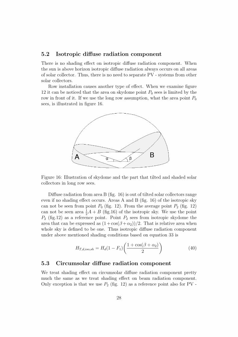
Row installation causes another type of effect. When we examine figure12 it can be noticed that the area on skydome point P0 sees is limited by therow in front of it. If we use the long row assumption, what the area point P0

sees, is illustrated in figure 16.

Figure 16: Illustration of skydome and the part that tilted and shaded solarcollectors in long row sees.

Diffuse radiation from area B (fig. 16) is out of tilted solar collectors rangeeven if no shading effect occurs. Areas A and B (fig. 16) of the isotropic skycan not be seen from point P0 (fig. 12). From the average point P2 (fig. 12)can not be seen area 1

2A + B (fig.16) of the isotropic sky. We use the point

P2 (fig.12) as a reference point. Point P2 sees from isotropic skydome thearea that can be expressed as (1+ cos(β+α2))/2. That is relative area whenwhole sky is defined to be one. Thus isotropic diffuse radiation componentunder above mentioned shading conditions based on equation 33 is

HT,d,iso,sh = Hd(1− F1)

(1 + cos(β + α2)

2

)(40)

5.3 Circumsolar diffuse radiation component

We treat shading effect on circumsolar diffuse radiation component prettymuch the same as we treat shading effect on beam radiation component.Only exception is that we use P2 (fig. 12) as a reference point also for PV -

28

systems as we did for solar collectors in sec 5.1. Point P2 is used because it isthe average point on solar collector as it was explained in section 5.1. Also,it should be noted that in a real situation when the sun is above the horizoncircumsolar diffuse always ends up on whole area of solar collector. In ourmathematical approach we assume circumsolar diffuse coming from the samedirection as beam radiation and for that reason it seems that circumsolardiffuse end up on whole solar collector when sun’s altitude angle is higherthan α. In a real case circumsolar diffuse comes from the area around thesun and the intensity of it decreases when going further from the sun onskydome.

Thus, solution for shading effect on circumsolar diffuse is: circumsolardiffuse occurs on solar collector when profile angle αp is higher than α2 fromfigure 12. Thus, circumsolar radiation on tilted surface under shading effectis

HT,d,cs,sh = HT,d,cs ∗ SEcs (41)

where shading effect on circumsolar diffuse radiation component SEcs is de-fined as

SEcs =

1 when αp > α2

0 when αp 6 α2(42)

5.4 Horizontal diffuse radiation component

Because horizontal diffuse radiation comes from the horizon the row of collec-tors in front of a solar collector blocks the diffuse radiation when we use longrow assumption. Thus horizontal diffuse radiation ends up only on the firstrow of solar collectors. We suggest to use a factor 1/N, where N is number ofrows, to correlate the lack of horizontal diffuse radiation on the rows behindthe first one. This gives to the horizontal diffuse radiation component (fromequation 33) a form of

HT,d,hz,sh =1

NHT,d,hz = Hd

1

NF2 sin β (43)

5.5 Ground reflected radiation component

It is obvious that for the first row of solar collectors ground reflection occursin a normal way. For other rows there is not much of the ground reflectbecause a row in front of it shadows the ground. Effect of ground reflectingon tilted surface is in general case neglectible [4]. Effect on rows behindthe first one is much smaller. Thus, the rows behind the first one could beconsidered dropping out entirely of the examination. Assuming the ground

29

reflecting only for the first row, based on equation 33 we get ground reflectedradiation on tilted surface under shading conditions as

HT,r,sh = Hg1

Nρ

(1− cos β

2

)(44)

where N is the number of rows.

5.6 Total radiation on tilted surface under shading ef-fect

The total radiation on tilted surface when self shading effect occurs can nowbe summarized into one equation:

HT,sh = HbRbSEb +Hd(1− F1)

(1 + cos(β + α2)

2

)+HdF1

a

bSEcs

+Hd1

NF2 sin β +Hg

1

Nρ

(1− cos β

2

) (45)

For simplicity in future, different terms in previous equation are expressedas

HT,sh = HT,b,sh +HT,d,iso,sh +HT,d,cs,sh +HT,d,hz,sh +HT,r,sh (46)

30

6 Effect of glass cover and dust

This far we have been pointing out the calculation methods to calculateradiation on some surface. The surface could be a plank of wood, a plasmatelevision or a solar collector. In case of solar collectors we must bring out areally important point: almost all solar collectors, whether they are PV - cellsor solar heat collectors, are covered by glass or some other material of thistype. The amount of radiation which passes the glass is strongly dependenton the angle of incidence (see fig 14). Effect of the angle of incidence to therelative transmittance can be expressed as

FT (θ) = 1− b0(

1

cos θ− 1

)(47)

where FT is the relative transmittance so that FT for normal orientatedbeam (θ = 0) is 1, θ is angle of incidence and b0 is a constant that is relatedto the characteristics of the surface of the solar collector [4]. When b0 is aunknown then general value b0 = 0.07 can be used [4].

Also dust has an effect on transmittance of solar collectors surface and itis really realistic to assume that a solar collector which is on use is coveredwith dust. Dust has two kind of effects on transmittance: The other effectis relative to the degree of dirtiness of solar collector and the another effectdepends on dirtiness level of solar collector and angle of incidence.

Parameter degree of dirtiness can be expressed as

Tdirt(0)/Tclean(0) =Transmittance of dirt surface

Transmittance of clean surface(48)

where zero stands for θ = 0. Thus Tdirt(0) is a normal orientated transmit-tance for a dirt surface and Tclean(0) is a normal orientated transmittance fora clean surface. Some classifications for the degree of dirtiness can be foundfrom table 6.

Table 6: Empirically adjusted parameters to take into account the effect ofglass cover and dust [4].

Dirtiness Tdirt(0)/Tclean(0) ar crClean 1 0.17 -0.069Low 0.98 0.20 -0.054Medium 0.97 0.21 -0.049High 0.92 0.27 -0.023

Degree of dirtiness and angle of incidence effect on relative transmittanceof surface of solar collector can be expressed for beam radiation component

31

as

FTb = 1−exp

(− cos θ

ar

)− exp

(− 1

ar

)1− exp

(− 1

ar

) (49)

where parameter ar is related to degree of dirtiness and can be found in table6. Because we assume circumsolar diffuse radiation component coming fromthe same direction as the beam radiation component, we use equation 49also for estimating dirtiness and glass cover effect on circumsolar radiationcomponent. Thus FTcs = FTb.

For isotropic diffuse radiation component relative transmittance can beexpressed as

FTd = 1− exp

[− 1

ar

[4

3π

(sin β +

π − β π

180− sin β

1 + cos β

)

+ cr

(sin β +

π − β π

180− sin β

1 + cos β

)2]] (50)

and for ground reflected radiation component relative transmittance can beexpressed as

FTr = 1− exp

[− 1

ar

[4

3π

(sin β +

βπ

180− sin β

1− cos β

)

+ cr

(sin β +

βπ

180− sin β

1− cos β

)2]] (51)

where dirtiness level related constants ar and cr can be found from table 6.Equations 49, 50 and 51 are from reference [11]. Unfortunately, relative

transmittance for horizontal diffuse radiation component was not suggested.Our suggestion for upper limit for relative transmittance for horizontal diffuseradiation is to modify the equation 49 so that

FThz(max) = 1−exp

(− cos(90− β)

ar

)− exp

(− 1

ar

)1− exp

(− 1

ar

) (52)

The equation is in the above form because horizontal diffuse radiation isparallel with horizon and thus the smallest angle of incidence it can come

32

across with tilted surface is 90o−β. Considering the neglectible role of Hd,hz

in HT we suggest that FThz(max) ≈ FThz.Now the total radiation on tilted surface taking account the effect of glass

cover and dust is

HT,FT =Tdirt(0)

Tclean(0)(HT,bFTb +HT,d,isoFTd +HT,d,csFTcs

+HT,d,hzFThz +HT,rFTr)

(53)

For simplicity in future we label components from previous equation withfollowing subscripts

HT,FT = HT,b,FT +HT,d,iso,FT +HT,d,cs,FT +HT,d,hz,FT +HT,r,FT (54)

33

7 Photovoltaic generation

So far we have got the tools to calculate irradiation on tilted surface andirradiation on a solar collector, which has been covered by glass and dust.With these tools we can calculate optimum tilt and orientation angle forsolar collector in general. In case of photovoltaic systems the ability of PV-system to transfer radiation into electricity needs to be taken into account.In following sections we present methods for that.

7.1 One diode equivalent circuit model

Solar cells have p-n-junction and it can be considered as a kind of diode.When there is no radiation on a solar cell it can be described as a diode.Electrical behavior of solar cell, which is under illumination conditions, canbe described with the circuit in fig 17 [6]. Current IPh is so called photocurrent and it is dependent on radiation.

Figure 17: One diode circuit equivalent solar cell that is under illumination[6]

In practical case charge carriers suffer a voltage drop through the p-n-junction of a semiconductor. The voltage drop can be described with theseries resistance Rs in figure 18 . Also, there is a small current leak involvedin edges of the solar cell. That can be described with parallel resistance Rp

in figure 18.Using Kirchhoff’s first rule on figure 18 circuit we get

0 = IPh − ID − IP − I (55)

Using symbols from figure 18 diode current ID can be expressed as ID =IS(exp(VD/mVt) − 1) where IS is the diode’s saturation current, m is the

34

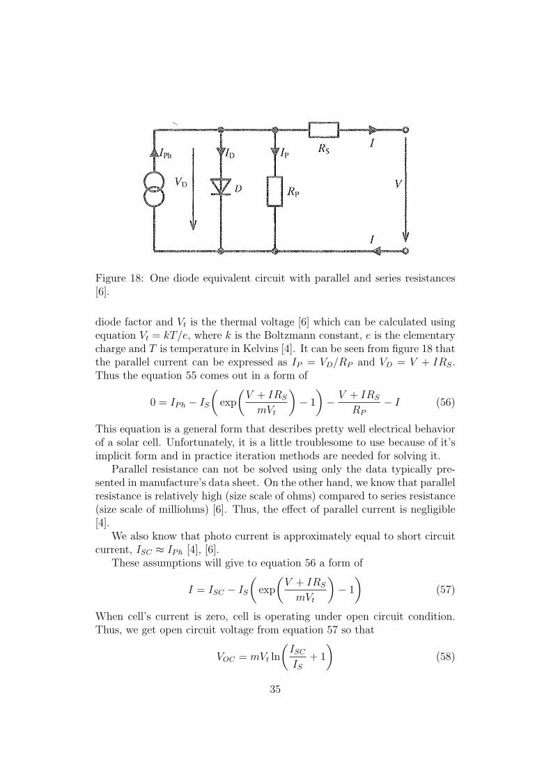
Figure 18: One diode equivalent circuit with parallel and series resistances[6].

diode factor and Vt is the thermal voltage [6] which can be calculated usingequation Vt = kT/e, where k is the Boltzmann constant, e is the elementarycharge and T is temperature in Kelvins [4]. It can be seen from figure 18 thatthe parallel current can be expressed as IP = VD/RP and VD = V + IRS.Thus the equation 55 comes out in a form of

0 = IPh − IS(

exp

(V + IRS

mVt

)− 1

)− V + IRS

RP

− I (56)

This equation is a general form that describes pretty well electrical behaviorof a solar cell. Unfortunately, it is a little troublesome to use because of it’simplicit form and in practice iteration methods are needed for solving it.

Parallel resistance can not be solved using only the data typically pre-sented in manufacture’s data sheet. On the other hand, we know that parallelresistance is relatively high (size scale of ohms) compared to series resistance(size scale of milliohms) [6]. Thus, the effect of parallel current is negligible[4].

We also know that photo current is approximately equal to short circuitcurrent, ISC ≈ IPh [4], [6].

These assumptions will give to equation 56 a form of

I = ISC − IS(

exp

(V + IRS

mVt

)− 1

)(57)

When cell’s current is zero, cell is operating under open circuit condition.Thus, we get open circuit voltage from equation 57 so that

VOC = mVt ln

(ISC

IS+ 1

)(58)

35

Solving saturation current from equation 58 we get

IS =ISC

exp

(VOC

mVT

)− 1

(59)

Adding equation 59 in equation 57 we get

I = ISC−ISC

exp

(V + IRS

mVt

)− 1

exp

(VOC

mVT

)− 1

≈ ISC

[1−exp

(V + IRS − VOC

mVt

)](60)

Constant m in equation 60 is a diode factor. Here we use as a diode factorthe ideal diode factor that is m = 1. That is adequate for describing theI-V behavior of solar cell even if it slightly overestimates the I and the V [4].This being the case

I = ISC

[1− exp

(V + IRS − VOC

Vt

)](61)

This equation describes I-V behavior of a solar cell [4]. Comparing to equa-tion 56 the equation 61 is still implicit and thus cumbersome to use but onthe other hand all parameters in it can be approximated using informationof solar cells from manufacturer data sheet and information about radiationand weather conditions [4].

In many cases solar cell’s open circuit voltage VOC , short circuit currentIOC , operation voltage at the maximum power point VMPP and operationcurrent at the maximum power point IMPP are given under standard testconditions (STC) by manufacture’s data sheet. Series resistance RS is tem-perature dependent but its temperature dependence is neglectible [6]. Refer-ence [4] suggest that RS is unaffected by the operation conditions. Thus wecan estimate RS from equation 61 in all radiation and weather conditions tobe

RS =

VOC,STC − VM,STC + Vt ln

(1− IM,STC

ISC,STC

)IM,STC

(62)

where subscript STC refers to data at standard test conditions, which canbe found from manufacture’s data sheet. Thermal voltage Vt can be foundby using (273.15 + 25) K as a temperature T which is temperature understandard test conditions.

To define I-V characteristics of solar cells using equation 61, the parame-ters VOC and ISC are also needed. Methods to find them under real operationconditions are presented in the following sections.

36

7.2 Short circuit current ISC under real operation con-ditions

Short circuit current is dependent on cell temperature. Increase in cell tem-perature causes increase in short circuit current. Dependence can be ex-pressed with temperature coefficient value for current αI which usually canbe found from manufacture’s data sheet. The temperature dependence forcurrent (TDI) can be expressed with following equation

TDI = 1 + αI(Tc − TSTC) (63)

where Tc is a cell temperature and TSTC is the temperature at standard testconditions, that is 25oC [6]. Typical value-range for αI is between 10−3/oCand 10−4/oC.

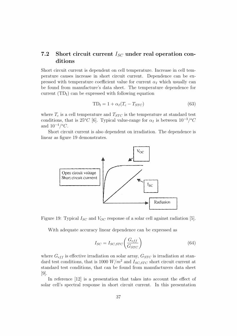
Short circuit current is also dependent on irradiation. The dependence islinear as figure 19 demonstrates.

Figure 19: Typical ISC and VOC response of a solar cell against radiation [5].

With adequate accuracy linear dependence can be expressed as

ISC = ISC,STC

(Geff

GSTC

)(64)

where Geff is effective irradiation on solar array, GSTC is irradiation at stan-dard test conditions, that is 1000 W/m2 and ISC,STC short circuit current atstandard test conditions, that can be found from manufacturers data sheet[9].

In reference [12] is a presentation that takes into account the effect ofsolar cell’s spectral response in short circuit current. In this presentation

37

Geff from equation 64 can be replaced with the following equation

Geff = Gbfb +Gdfd +Grfr (65)

where fb, fd and fr can be found from equation

fi = ci exp[ai(kT − 0.74) + bi(AM − 1.5)] (66)

Empirically adjusted parameters a, b and c take into account the differentirradiation components. For monocrystalline solar cell the parameters canbe found from table 7, for polycrystalline solar cell the parameters can befound from table 8 and for amorphous silicon solar cells the parameters canbe found from table 9.

Table 7: Empirical factors to estimate spectral response of a monocrystallinesolar cell [12].

Hb Hd Hr

a −3.13 ∗ 10−1 −8.82 ∗ 10−1 −2.44 ∗ 10−1

b 5.24 ∗ 10−3 −2.04 ∗ 10−2 1.29 ∗ 10−3

c 1.029 0.764 0.970

Table 8: Empirical factors to estimate spectral response of a polycrystallinesolar cell [12].

Hb Hd Hr

a −3.11 ∗ 10−1 −9.29 ∗ 10−1 −2.70 ∗ 10−1

b 6.26 ∗ 10−3 −1.92 ∗ 10−2 1.58 ∗ 10−2

c 1.029 0.764 0.970

Table 9: Empirical factors to estimate spectral response of a amorphoussilicon solar cell [12].

Hb Hd Hr

a −2.22 ∗ 10−1 −7.28 ∗ 10−1 −2.19 ∗ 10−1

b 9.20 ∗ 10−3 −1.83 ∗ 10−2 1.79 ∗ 10−2

c 1.024 0.840 0.989

Summarizing the temperature effect and the spectral effect in equation64 we get

ISC = ISC,STC [1 + αI(Tc − TSTC)]

(Gbfb +Gdfd +Grfr

GSTC

)(67)

38

7.3 Open circuit voltage under real operation condi-tions

Open circuit voltage is temperature dependent. Increase in cell’s temperaturecauses a decrease in cell’s open circuit voltage. The temperature dependency(TDV) can be expressed as

TDV = 1 + αV (Tc − TSTC) (68)

where αV is temperature coefficient for voltage and TSTC is the temperatureat standard test conditions, that is 25oC [6]. The temperature coefficient αV

can be found from manufacturer’s data sheet. Typical value-range for αV incase of silicon solar cell is between −3 ∗ 10−3/oC and −5 ∗ 103/oC [6].

Irradiation level has also effect on open circuit voltage. It seems thathigher irradiation causes higher open circuit voltage. Unlike in case of theshort circuit current the dependence is not linear. Using the equation 64and by making the assumptions that ISC,STC/IS 1, we can derive fromequation 58 irradiation effect on open circuit voltage. The derivation hasbeen done in reference [9] and the result is

VOC = VOC,STC +mVt ln

(Geff

GSTC

)(69)

where Geff is an effective irradiation. This logarithmic dependence of irradi-ation is derived from equations based on one diode equivalent circuit model.Even though one diode model is the best we can have if we want to useinput data only from the manufacture’s data site, its weakness is solar cellsbehavior under low irradiation conditions. References [4] and [9] report thatirradiation level dropping under 200 W/m2 can cause significant drop in opencircuit voltage.

At low irradiation conditions recombination rate in p-n junction starts toplay a significant role [9]. If photo-current drops near to the recombinationcurrent, the open circuit voltage suffers a significant drop. Figure 19 illus-trates the open circuit voltage behavior at different irradiation levels. Onediode model does not take into account the open circuit voltage drop at lowirradiation levels.

Reference [9] suggest to add second logarithmic term in equation 69 tofix the low irradiation behavior problem in one diode model. Unfortunately,the logarithmic term includes two parameters which need to be found outempirically. In essence of this study we can not use the term. Reference[4] and reference therein [18] suggest a similar type of two-logarithmic termthat also includes two unknown parameters which need to be found out

39

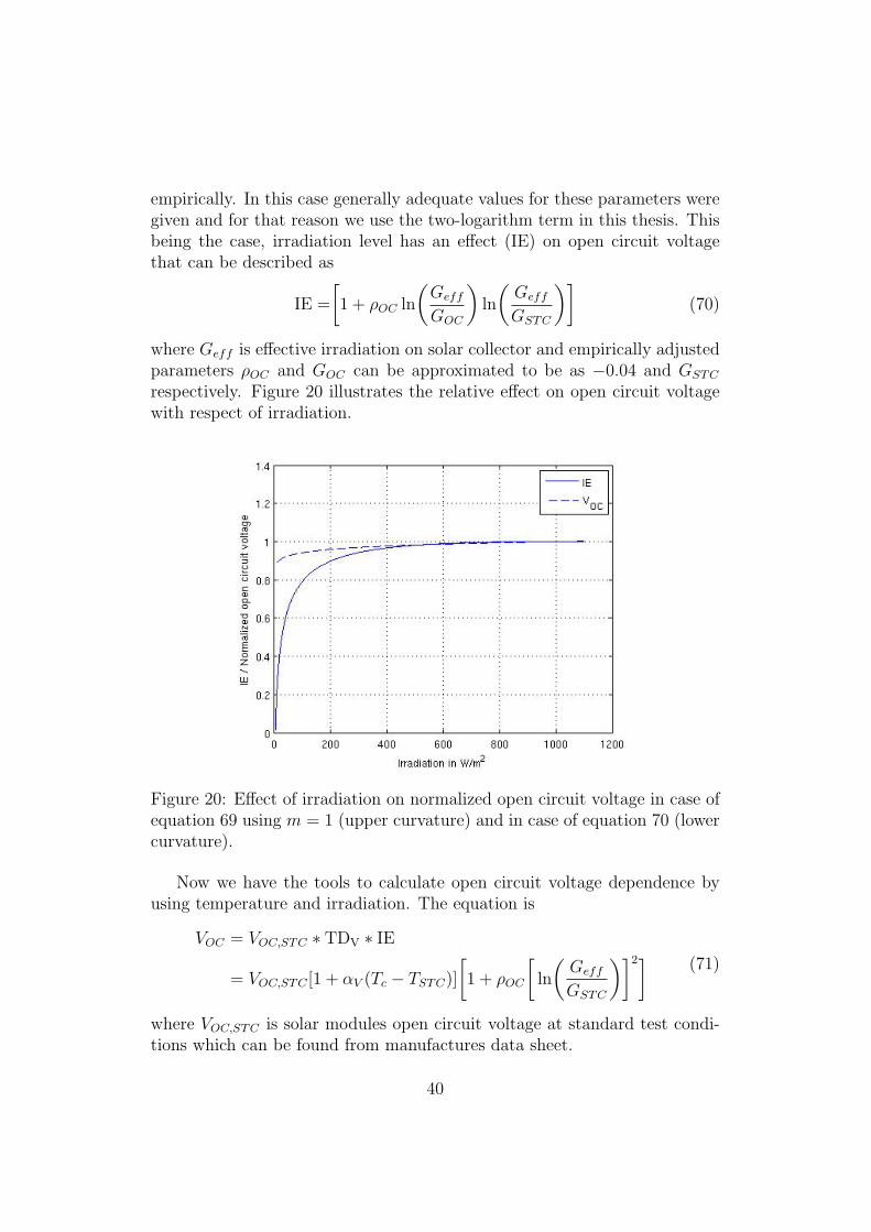
empirically. In this case generally adequate values for these parameters weregiven and for that reason we use the two-logarithm term in this thesis. Thisbeing the case, irradiation level has an effect (IE) on open circuit voltagethat can be described as

IE =

[1 + ρOC ln

(Geff

GOC

)ln

(Geff

GSTC

)](70)

where Geff is effective irradiation on solar collector and empirically adjustedparameters ρOC and GOC can be approximated to be as −0.04 and GSTC

respectively. Figure 20 illustrates the relative effect on open circuit voltagewith respect of irradiation.

Figure 20: Effect of irradiation on normalized open circuit voltage in case ofequation 69 using m = 1 (upper curvature) and in case of equation 70 (lowercurvature).

Now we have the tools to calculate open circuit voltage dependence byusing temperature and irradiation. The equation is

VOC = VOC,STC ∗ TDV ∗ IE

= VOC,STC [1 + αV (Tc − TSTC)]

[1 + ρOC

[ln

(Geff

GSTC

)]2] (71)

where VOC,STC is solar modules open circuit voltage at standard test condi-tions which can be found from manufactures data sheet.

40

7.4 Cell temperature

Information about cell temperature is needed for calculating short circuitcurrent ISC , open circuit voltage VOC and thermal voltage Vt. Some methodsfor finding cell temperature are presented next.

7.4.1 Using NOCT

Ambient temperature and irradiation have effect on cell temperature. Theeffect can be described with following equation

Tc,NOCT = Ta + CtGeff (72)

where Tc,NOCT is the cell temperature, Ta is the ambient temperature, Geff

is the effective irradiation on surface and constant Ct is

Ct =NOCT (oC)− 20

800W/m2(73)

where NOCT is normal operating cell temperature and generally can befound from manufacturer’s data sheet [4]. Typical value is in range of 42oCto 46oC. When NOCT is unknown approximation Ct = 0.030oC/(W/m2)is reasonable [4]. When using NOCT value from manufacturer’s data sheetit is expected that air can flow from the front and the back side of the solarmodule. If only partial flow from back side is allowed, NOCT can rise 17oCand if back side is fully restricted from airflow, like in the case of some roofinstallations, NOCT can rise 35oC.

7.4.2 Using wind speed

Wind speed has also effect on cell temperature. Luque et al. [4] referring toRef. [19] suggest that it can be expressed as

Tc,wind = Tm +Geff

GSTC

4 T (74)

where Tm is back surface temperature of solar module and can be expressedas

Tm = Ta +Geff

GSTC

[T1 exp(b ∗ uS) + T2] (75)

where uS is the wind speed. Empirically adjusted parameters 4T , T1, T2,and b can be found from table 10.

41

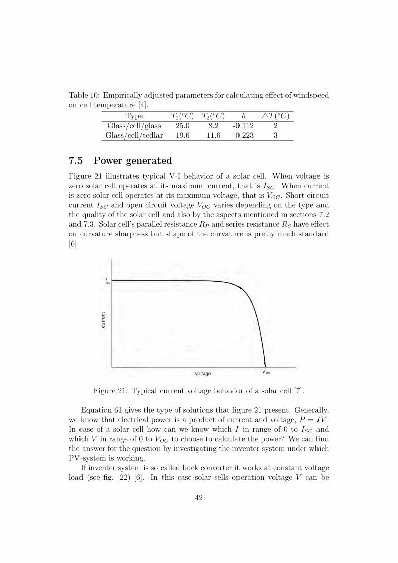
Table 10: Empirically adjusted parameters for calculating effect of windspeedon cell temperature [4].

Type T1(oC) T2(

oC) b 4T (oC)Glass/cell/glass 25.0 8.2 -0.112 2Glass/cell/tedlar 19.6 11.6 -0.223 3

7.5 Power generated

Figure 21 illustrates typical V-I behavior of a solar cell. When voltage iszero solar cell operates at its maximum current, that is ISC . When currentis zero solar cell operates at its maximum voltage, that is VOC . Short circuitcurrent ISC and open circuit voltage VOC varies depending on the type andthe quality of the solar cell and also by the aspects mentioned in sections 7.2and 7.3. Solar cell’s parallel resistance RP and series resistance RS have effecton curvature sharpness but shape of the curvature is pretty much standard[6].

Figure 21: Typical current voltage behavior of a solar cell [7].

Equation 61 gives the type of solutions that figure 21 present. Generally,we know that electrical power is a product of current and voltage, P = IV .In case of a solar cell how can we know which I in range of 0 to ISC andwhich V in range of 0 to VOC to choose to calculate the power? We can findthe answer for the question by investigating the inventer system under whichPV-system is working.

If inventer system is so called buck converter it works at constant voltageload (see fig. 22) [6]. In this case solar sells operation voltage V can be

42

chosen to be same as inverters voltage load. In case of figure 22 that wouldbe V1. Now operating current for that certain voltage can be calculated usingequation 61 and further more the operating power.

Figure 22: Illustration of buck converter’s constant voltage load [6].

More common and definitely better inventer type is the so called max-imum power point tracker. MPP tracker finds and operates at the voltagewhere product of IV generates its maximum value [6]. The point is calledas maximum power point, MPP.

Solar cell V-I behavior and product of I and V are presented in figure 23.In case of figure 23 MPP tracker type of inventer would operate at voltagethat is VMPP . That certain operation voltage is called maximum powerpoint voltage and we can find maximum power point current IMPP by usingequation 61. Product of IMPP and VMPP gives the maximum power pointpower PMPP which we assume to be the solar cells operation power. Wecan generalize this in the following way: When assuming PV-system workingunder MPP tracer type of inventer we can define system power PMPP usingthe equation 61 in a following way

I = ISC

[1− exp

(V + IRS − VOC

Vt

)]P = IV

PMPP = max (P )

(76)

43

Figure 23: Solar cell’s V-I and V-P behavior [6].

8 Results

8.1 Case Pitajanmaki

In this section I have calculated the theoretical yield of solar array plannedin Pitajanmaki. At the end of this section the yield is calculated for a rangeof tilt and orientation angles to find out the tilt and orientation angles thatlead to the greatest yield.

8.1.1 Example calculation: radiation on tilted surface

To illustrate the calculation method described in this thesis, the day of07.08.2007 is chosen to be an example day. To receive final results, all thedays from the three year data are calculated similarly like the example day.Day 07.08.2007 have been chosen randomly just to illustrate the steps of thewhole calculation.

The day number for this example day is n = 189 and thus the declinationfor this day using equation 1 is δ = 23.448o. The direction of our examplesolar collector was chosen so that its orientation angle γ = 20o and its tiltangle β = 30o. The organization which is planning to build up the solararray informed us that collectors are needed to be orientated 20o from southto west. For this reason the orientation angle for the example calculationwas chosen to be γ = 20o. On the other hand, the sales manager of SulwindGylling Oy was informed by an expert that the optimum tilt angle for thisarray might be 30o. For this reason the tilt angle for this example calculationwas chosen to be β = 30o.

44

The hours of the example day are presented in column TO in table 11 sothat given hour is a starting point of the measured hour. For example hour14 represents data which is measured from 14:00 to 15:00.

Global radiation, diffuse radiation, average ambient temperature and av-erage wind speed for the given hour are in columns Hg, Hd, Ta and uS,respectively. These parameters are from the data of FMI and thus radiationparameters are for horizontal surface. Beam radiations are calculated as thedifference between global and diffuse radiations, Hb = Hg −Hd.

Hour angles are in column ω1 and they were calculated using equation4. Subscript 1 tells that the given hour angle is the starting point of themeasured hour. Some equations require ω2 which is the ending point ofthe measured hour. However, it can simply be calculated as follows: ω2 =ω1 + 15o. Solving ω2 for the last hour of the day from the equation, givesan incorrect value. However, we ignore this because the last hour of the dayis at midnight and at that time no radiation occurs. Some of the equationsrequire parameter ω and the middle points of the measured hours are chosenas values for these parameters. Thus ω = ω1 + 7.5o.

Extraterrestrial radiations on horizontal surface for each hour are cal-culated from equation 13 and are in column H0 and the clearness indicesare calculated using equation 14 and are in column kT . Unsteady weatherconditions of our example summer day can be seen in the clearness indices.The values higher than 0.8 represent clear sky, the values below 0.22 rep-resent heavily over-casted sky and the values between these two representthe intermediate sky conditions. Extraterrestrial radiations are negative atsolar night hours and they give a negative value for clearness indices at solarnight hours. Negative clearness indices are not listed in table 11 and theyare replaced with zeros.

If for some reason Hglobal,hor > H0 then clearness index gets a value higherthan one. These are unphysical situations and in these cases kT are chosen tobe one. Hour 20 in table 11 represents this kind of situation. In overall datathe situation Hglobal,hor > H0 happens only during sunset and sunrise hours.At these hours radiation is relatively small and thus the effect of uncertainclearness index is neglectible.

In columns cos θ and cos θz are values which are solved from equations 5and 6, using values from tables 1 and 11 and parameters δ = 23.448o, β = 30o

and γ = 20o . Values in column Rb were calculated using equation 19 exceptfor sunrise and sunset hours using equation 20.

Clearness ε was calculated using cos θz in equation 26. Atmosphericbrightness ∆ was calculated using equation 29 using equations 9 and 10.Clearness and atmospheric brightness are in columns ε and ∆. Using clear-ness ε the correct values were found for brightness coefficients f11, f12, f13,

45

f21, f22 and f23 from table 5. Values in columns F1 and F2 of table 11 werecalculated using equations 27 and 28 with ∆, f11, f12, f13, f21, f22 and f23.

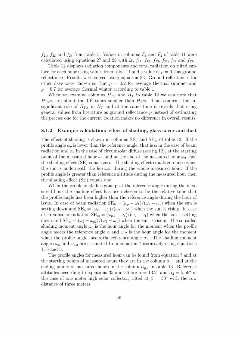
Table 12 displays radiation components and total radiation on tilted sur-face for each hour using values from table 11 and a value of ρ = 0.2 as groundreflectance. Results were solved using equation 33. Ground reflectances forother days were chosen so that ρ = 0.2 for average thermal summer andρ = 0.7 for average thermal winter according to table 1.

When we examine columns HT,r and HT in table 12 we can note thatHT,r:s are about the 102 times smaller than HT :s. That confirms the in-significant role of HT,r in HT and at the same time it reveals that usinggeneral values from literature as ground reflectance ρ instead of estimatingthe precise one for the current location makes no difference in overall results.

8.1.2 Example calculation: effect of shading, glass cover and dust

The effect of shading is shown in columns SEb and SEcs of table 13. If theprofile angle αp is lower than the reference angle, that is α in the case of beamradiation and α2 in the case of circumsolar diffuse (see fig 12), at the startingpoint of the measured hour ω1 and at the end of the measured hour ω2 thenthe shading effect (SE) equals zero. The shading effect equals zero also whenthe sun is underneath the horizon during the whole measured hour. If theprofile angle is greater than reference altitude during the measured hour thenthe shading effect (SE) equals one.

When the profile angle has gone past the reference angle during the mea-sured hour the shading effect has been chosen to be the relative time thatthe profile angle has been higher than the reference angle during the hour ofissue. In case of beam radiation SEb = (ωp − ω1)/(ω2 − ω1) when the sun issetting down and SEb = (ω2 − ωp)/(ω2 − ω1) when the sun is rising. In caseof circumsolar radiation SEcs = (ωp,2−ω1)/(ω2−ω1) when the sun is settingdown and SEcs = (ω2 − ωp2)/(ω2 − ω1) when the sun is rising. The so calledshading moment angle ωp is the hour angle for the moment when the profileangle meets the reference angle α and ωp2 is the hour angle for the momentwhen the profile angle meets the reference angle α2. The shading momentangles ωp and ωp,2 are estimated from equation 7 iteratively using equations1, 6 and 8.

The profile angles for measured hour can be found from equation 7 and atthe starting points of measured hours they are in the column αp,1 and at theending points of measured hours in the column αp,2 in table 13. Referencealtitudes according to equations 35 and 36 are α = 13.2o and α2 = 5.56o inthe case of one meter high solar collector, tilted at β = 30o with the rowdistance of three meters.

46

Tab

le11

:V

alues

from

the

FM

Idat

abas

ean

dva

lues

that

wer

enee

ded

for

calc

ula

ting

hou

rly

radia

tion

onti

lted

surf

ace

(β=

30o

andγ

=20

o)

and

for

phot

oval

atic

calc

ula

tion

son

7:th

Augu

st20

07(n

=18

9).

AllH

:sar

einkJ/m

2.

TO

Hg

Hd

Ta(oC

)u

S(m

s)

Hb

ω1(deg.)

H0

kT

cosθ

cosθ z

Rb

ε∆

F1

F2

00

015

.33.

80

-171

.62

-523

0-0

.591

-0.1

110

-0

00

10

015

.33.

60

-156

.62

-297

0-0

.549

-0.0

640

-0

00

214

1215

.13.

32

-141

.62

570.

245

-0.4

550.

011

04.

036

0.22

70.

208

0.18

83

5754

15.3

3.3

3-1

26.6

251

50.

111

-0.3

180.

108

01.

121

0.10

60

-0.0

544

115

111

15.1

3.2

4-1

11.6

210

450.

110

-0.1

450.

219

01.

046

0.10

60

-0.0

825

268

264

15.2

1.6

4-9

6.62

1612

0.16

60.

052

0.33

90.

152

1.01

50.

164

0.01

2-0

.075

640

439

915

.42

5-8

1.62

2176

0.18

60.

258

0.45

80.

563

1.01

20.

183

0.03

2-0

.071

757

656

715

.82

9-6

6.62

2699

0.21

30.

460

0.56

80.

810

1.01

40.

210

0.05

5-0

.066

896

995

017

2.5

19-5

1.62

3147

0.30

80.

644

0.66

20.

973

1.01

80.

301

0.11

7-0

.057

974

573

317

1.8

12-3

6.62

3487

0.21

40.

798

0.73

41.

087

1.01

60.

210

0.06

9-0

.061

1014

9214

1418

.11.

678

-21.

6236

970.

404

0.91

10.

778

1.17

11.

053

0.38

20.

174

-0.0

4711

1989

1321

202

668

-6.6

237

630.

529

0.97

50.

792

1.23

11.

493

0.35

00.

362

0.01

512

985

832

17.9

2.8

153

8.38

3680

0.26

80.

986

0.77

41.

274

1.17

80.

226

0.18

1-0

.024

1322

7195

218

.81.

513

1923

.38

3453

0.65

80.

944

0.72

71.

299

2.31

30.

275

0.49

10.

100

1425

6373

421

.22.

218

2938

.38

3099

0.82

70.

851

0.65

21.

305

3.29

80.

237

0.48

50.

142

1511

3965

019

.63.

848

953

.38

2641

0.43

10.

713

0.55

61.

283

1.68

20.

246

0.32

40.

058

1618

1379

720

.12.

510

1668

.38

2111

0.85

90.

540

0.44

41.

217

2.18

30.

377

0.32

30.

053

1712

1543

919

.83.

777

683

.38

1545

0.78

70.

344

0.32

51.

059

2.82

40.

284

0.26

90.

124

1844

723

418

.33.

621

398

.38

980

0.45

60.

138

0.20

60.

669

2.21

60.

239

0.28

60.

117

1986

8116

.93.

45

113.

3845

70.

188

-0.0

650.

095

01.

149

0.17

90.

029

-0.0

5020

1817

162.

81

128.

3810

1-0

.249

0.00

10

11.5

083.

207

0-3

.866

210

015

.52

014

3.38

-330

0-0

.403

-0.0

710

-0

00

220

015

.32.

50

158.

38-5

410

-0.5

15-0

.115

0-

00

023

00

14.8

1.9

017

3.38

-606

0-0

.580

-0.1

290

-0

00

47

Table 12: Radiation components to tilted surface (β = 30o and γ = 20o)on 7:th August 2007, using as a ground reflectance ρ = 0.2. All H:s are inkJ/m2.

TO HT,b HT,iso HT,cs HT,hz HT,r HT

0 0 0 0 0 0 01 0 0 0 0 0 02 0 9 0 1 0 103 0 50 0 -1 1 504 0 104 0 -5 2 1015 1 243 0 -10 4 2386 3 360 7 -14 5 3627 7 500 25 -19 8 5218 18 783 108 -27 13 8959 13 637 55 -22 10 69210 91 1089 289 -34 20 145611 823 786 589 10 27 223512 195 636 192 -10 13 102613 1713 452 607 47 30 285114 2386 353 464 52 34 329015 627 410 271 19 15 134216 1236 503 313 21 24 209817 822 299 125 27 16 129018 143 156 45 14 6 36319 0 73 0 -2 1 7220 0 16 0 -33 0 021 0 0 0 0 0 022 0 0 0 0 0 023 0 0 0 0 0 0

Relative transmittances for isotropic diffuse, horizontal diffuse and groundreflectance are functions of β and dirtiness level from table 6. In this casedirtiness level is chosen to be Medium and tilt angle β = 30o. Thus, rela-tive transmittances for above mentioned radiation components are FTiso =0.9315, FThz = 0.9154 and FTr = 0.7163. Relative transmittances for beamradiation components and circumsolar radiation components are the sameFTb = FTcs, which is explained in section 6. The parameters FTb and FTcs

are functions of cos θ and thus they vary at every hour. Values for FTb andFTcs are calculated using equation 49 and are in the column FTb&FTcs oftable 13.

48

When examining the table 13 it seems like SEb and SEcs have no effectbecause FTb and FTcs are nonzero only when SE = 1, which is true for thisgiven day and given tilt and orientation angle. For example a higher tiltangle would give less zeros in FT column and more zeros in SE columns, anda lower tilt angle would give less zeros in SE columns and more zeros in FTcolumn. In other words, as the chosen tilt angle is near to the optimum tiltangle(we will find out that later) FE and SE get nonzero values pretty muchat the same hours.

Table 13: Values that describe effect of shading, glass cover and dust. Theparameters αp,1 and αp,2 are in degrees.

TO αp,1 αp,2 SEb SEcs FTb&FTcs

0 7.28 5.22 0 0 01 5.22 1.74 0 0 02 1.74 3.70 0 0 03 3.70 12.18 0 0.738 04 12.18 25.66 0.907 1 05 25.66 46.22 1 1 0.2196 46.22 71.67 1 1 0.7137 71.67 86.23 1 1 0.8968 86.23 71.34 1 1 0.9629 71.34 61.97 1 1 0.98610 61.97 55.98 1 1 0.99511 55.98 52.14 1 1 0.99912 52.14 49.79 1 1 0.99913 49.79 48.74 1 1 0.99714 48.74 49.17 1 1 0.99115 49.17 51.96 1 1 0.97516 51.96 60.04 1 1 0.93217 60.04 84.83 1 1 0.81218 84.83 38.43 1 1 0.48519 38.43 6.55 0.674 1 020 6.55 3.65 0 0.061 021 3.65 7.20 0 0 022 7.20 8.03 0 0 023 8.03 8.03 0 0 0

Table 14 shows radiation components and total radiation on tilted solarcollector for each hour when taking into account shading effect, glass coverand dust. Results were solved from equations 45 and 53 using values from

49

previous tables in this section.

Table 14: Effective radiation components on tilted solar collector. H:s are inkJ/m2.

TO HT,b,sh,FT HT,iso,sh,FT HT,cs,sh,FT HT,hz,sh,FT HT,r,sh,FT HT,sh,FT

0 0 0 0 0 0 01 0 0 0 0 0 02 0.0 7.8 0.0 0.0 0.0 7.83 0.0 44.2 0.0 0.0 0.0 44.24 0.0 90.9 0.0 -0.1 0.0 90.95 0.1 213.6 0.1 -0.2 0.0 213.76 1.9 316.5 4.9 -0.3 0.1 323.27 6.3 438.8 22.1 -0.3 0.1 467.08 17.2 687.4 100.6 -0.5 0.2 805.09 12.5 559.0 52.7 -0.4 0.1 623.910 88.2 956.4 278.8 -0.6 0.3 1323.011 797.0 690.4 570.7 0.2 0.4 2058.612 188.9 558.4 185.7 -0.2 0.2 933.113 1657.7 397.0 587.4 0.8 0.4 2643.414 2293.9 309.8 446.4 0.9 0.5 3051.515 593.3 359.8 255.8 0.3 0.2 1209.416 1116.8 442.1 283.0 0.4 0.3 1842.617 647.7 262.8 98.7 0.5 0.2 1009.918 67.0 137.0 21.0 0.2 0.1 225.319 0.0 64.4 0.0 0.0 0.0 64.420 0.0 13.9 0.0 -0.6 0.0 13.321 0 0 0 0 0 022 0 0 0 0 0 023 0 0 0 0 0 0

8.1.3 Example calculation: photovoltaic generation

To find photovoltaic yield we need to calculate the open circuit voltage andshort circuit current at operating point. ISC and VOC can be found fromequations 67 and 71 but they require parameters Geff/GSTC , where Geff isan effective irradiation on solar collector and GSTC an irradiation at standardtest conditions, which is 1000 W/m2. Effective irradiation on solar collectorduring one hour is averagely same as effective radiation on solar collector

50

during one hour divided by 3600s, Geff = Heff/3600s. In our case effectiveradiation on solar collector is HT,sh,FT from table 14 and thus Geff/GSTC =(Heff/3600s)/GSTC = HT,sh,FT/(1000 W/m2 ∗ 3600 s). These values are intable 15 in column Geff/GSTC .

To calculate VOC and ISC we also need to know the cell temperature.Cell temperatures were calculated using two different theories. Cell tem-peratures from equation 72 were solved using NOTC = 46oC (table 2),Geff = HT,sh,FT/3600 s (table 14) and Ta (table 11) values. Cell tempera-tures are listed in column Tc,NOCT in table 15. Using NOCT value straightfrom manufacturers data is in this case reasonable because the whole solararray is planned to be build on stands and thus air can flow freely on bothsides of the solar collectors.

Cell temperatures from equation 74 are listed in column Tc,wind. Ambienttemperatures Ta here are also from table 11, same as wind speeds uS. Rest ofthe required values can be found from table 10 and table 15. Back surface ofthe Swedmodule GPV200 solar module is made of Tedlar (see table 2) [Ap-pendix 2]. Thus we can use values for Glass/cell/tedlar in table 10. Averagesof these cell temperatures found in two different ways are in column Tc intable 15. These values are used as cell temperature in further calculations.

Operating open circuit voltages are calculated using equation 71. ValuesVOC,STC = 36.6 V , αV = −0.0034/K and TSTC = 25oC were taken fromtable 2. The parameter ρOC = −0.04 as it has been described in section 7.3.Results are in column VOC of table 15. Equation 71 gives negative values forVOC at really low radiation conditions which happens when Geff/GSTC .0.007. Those values have been chosen to be zero because it is unrealistic toassume solar array acting as a energy consumer because of low irradiation.

Operating short circuit currents calculated using equation 67 are in col-umn ISC of table 15. Equation 67 requires values for ISC,STC , αI and TSTC

and the values can be found from table 2. Values for Tc can be foundfrom table 15 and values for Hb, Hd and Hr can be found from table 14so that Hb = HT,b,sh,FT , Hd = HT,iso,sh,FT + HT,cs,sh,FT + HT,hz,sh,FT andHr = HT,r,sh,FT . Equation 67 also requires values fb,fd and fr. They canbe found from equation 66 using the data of table 8 since the type of solarmodule system in issue is polycrystalline. Equation 66 also requires valuesfor clearness indices kT . They can be found from table 11.

Before we can calculate the operation powers of solar module we need onemore parameter and that is the series resistance of solar module. That can befound from equation 62 using values from table 2. When calculating RS fromequation 62 it has to be remembered that there is 60 solar cells in the GPV200module. The assumption is that all solar cells in the GPV200 module are inseries and thus we use as a diode factor m = 60 · (diode factor). We do not

51

have the information about diode factor of solar cell in the GPV200 module.On the other hand, reference [4] claims that it is reasonable to use diodefactor = ideal diode factor = 1 in this kind of calculations. Thus m = 60and using this we receive the result RS = 0.515 Ω [4].

Maximum operating powers of solar module were solved from equation76 iteratively and they are listed in table 15 in column PMPP . If we comparethis column to column Hg from table 11 we note that only radiation in scaleof 100 kJ/m2 in hour can cause reasonable power output from PV-system.Maximum Watt-peak power which is same as the operating power at standardtest conditions can be found from manufacturers data [Appendix 2] and itis 203.3 W . All operating powers in column PMPP are much smaller thanwatt peak power which describes the feebleness of real operating conditionscompared to standard test condition.

As it was planned to have the total of 700 modules in the whole solarpower plant system, the total energy output for each hour is Ehour = 700 ·PMPP · 3600 s. Those values are listed in the column Ehour of table 15.

Now we can calculate the total energy production for whole day (07.08.2007)and that is Eday =

∑23TO=0Ehour = 2.276 GJ .

8.1.4 Final result: tilt and orientation angle effect on yield

There was the total of 1096 days in the data from Finnish MeteorologicalInstitute (years 2007-2009). Matlab software [15] was used to calculate Eday

for all of the days, in the same way as it has been described previously in thissection. The total energy production for all the three year is E2007−2009 =∑1096

day=1Eday = 1.489 TJ . This result was received using the tilt angle β = 30o

and the orientation angle γ = 20o. Thus we define labeling E2007−2009(β =30o, γ = 20o) = 1.489 TJ .

When doing these calculation all over again with different tilt angles,in range of β = [0, 90o] and with different orientations, in range of γ =[−90o, 90o] we receive E2007−2009(β, γ). The result can be described best withfollowing 3D graph in figure 24.

Top of the mountain is 1.507 TJ high and its coordinates are β = 28.6o

and γ = 0.1o.The starting point requirement for orientation was that the rows needed

to be orientated in a direction of γ = 20o. Cross-section from figure 24 atpoint γ = 20o is illustrated in figure 25. The top of cross-section is at theheight of 1.489 TJ and it can be received with tilt angle β = 28.5o.

52

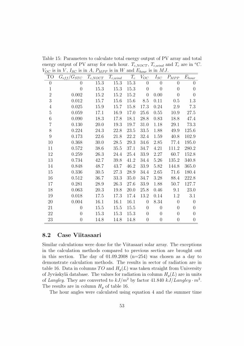
Table 15: Parameters to calculate total energy output of PV array and totalenergy output of PV array for each hour. Tc,NOCT , Tc,wind and Tc are in oC.VOC is in V , ISC is in A, PMPP is in W and Ehour is in MJ .

TO Geff/GSTC Tc,NOCT Tc,wind Tc VOC ISC PMPP Ehour

0 0 15.3 15.3 15.3 0 0 0 01 0 15.3 15.3 15.3 0 0 0 02 0.002 15.2 15.2 15.2 0 0.00 0 03 0.012 15.7 15.6 15.6 8.5 0.11 0.5 1.34 0.025 15.9 15.7 15.8 17.3 0.24 2.9 7.35 0.059 17.1 16.9 17.0 25.6 0.55 10.9 27.56 0.090 18.3 17.8 18.1 28.8 0.83 18.8 47.47 0.130 20.0 19.3 19.7 31.0 1.18 29.1 73.38 0.224 24.3 22.8 23.5 33.5 1.88 49.9 125.69 0.173 22.6 21.8 22.2 32.4 1.59 40.8 102.910 0.368 30.0 28.5 29.3 34.6 2.85 77.4 195.011 0.572 38.6 35.5 37.1 34.7 4.21 111.2 280.212 0.259 26.3 24.4 25.4 33.9 2.27 60.7 152.813 0.734 42.7 39.8 41.2 34.4 5.26 135.2 340.814 0.848 48.7 43.7 46.2 33.9 5.82 144.8 365.015 0.336 30.5 27.3 28.9 34.4 2.65 71.6 180.416 0.512 36.7 33.3 35.0 34.7 3.28 88.4 222.817 0.281 28.9 26.3 27.6 33.9 1.88 50.7 127.718 0.063 20.3 19.8 20.0 25.8 0.46 9.1 23.019 0.018 17.5 17.3 17.4 13.2 0.14 1.2 3.120 0.004 16.1 16.1 16.1 0 8.34 0 021 0 15.5 15.5 15.5 0 0 0 022 0 15.3 15.3 15.3 0 0 0 023 0 14.8 14.8 14.8 0 0 0 0

8.2 Case Viitasaari

Similar calculations were done for the Viitasaari solar array. The exceptionsin the calculation methods compared to previous section are brought outin this section. The day of 01.09.2008 (n=254) was chosen as a day todemonstrate calculation methods. The results in sector of radiation are intable 16. Data in columns TO and Hg(L) was taken straight from Universityof Jyvaskyla database. The values for radiation in column Hg(L) are in unitsof Langley. They are converted to kJ/m2 by factor 41.840 kJ/Langley ·m2.The results are in column Hg of table 16.

The hour angles were calculated using equation 4 and the summer time

53

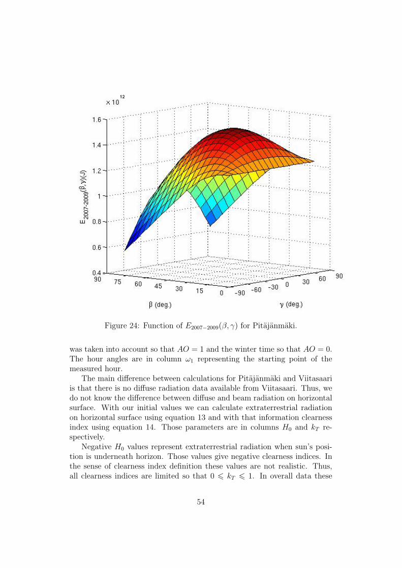
Figure 24: Function of E2007−2009(β, γ) for Pitajanmaki.

was taken into account so that AO = 1 and the winter time so that AO = 0.The hour angles are in column ω1 representing the starting point of themeasured hour.

The main difference between calculations for Pitajanmaki and Viitasaariis that there is no diffuse radiation data available from Viitasaari. Thus, wedo not know the difference between diffuse and beam radiation on horizontalsurface. With our initial values we can calculate extraterrestrial radiationon horizontal surface using equation 13 and with that information clearnessindex using equation 14. Those parameters are in columns H0 and kT re-spectively.

Negative H0 values represent extraterrestrial radiation when sun’s posi-tion is underneath horizon. Those values give negative clearness indices. Inthe sense of clearness index definition these values are not realistic. Thus,all clearness indices are limited so that 0 6 kT 6 1. In overall data these

54

Figure 25: Function of E2007−2009(β, γ = 20o) for Pitajanmaki.

exceptions occur sometimes in the first and last measured hour of the day. Inthose cases the sun was theoretically beneath the horizon but measurementsystem was still receiving some radiation. In this kind of situation choos-ing kT to be zero is reasonable since kt = 0 means that all measured globalradiation is considered to be as diffuse radiation in calculations (see fig 6).

By using clearness index kT we estimated diffuse radiation on horizontalsurface using equation 15. Results are in column Hd of table 16. Beamradiations on horizontal surface are Hb = Hg − Hd and they are in columnHb.

Figure 26 is here to demonstrate the way equation 15 works. All fourcurvatures were drawn using data from table 16. Clearly the morning wasclear and the noon was cloudy during the example day. In the morningglobal radiation is near to extraterrestrial radiation and at noon it is muchbelow the extraterrestrial radiation. Because in the morning there is a lot ofglobal radiation equation 15 expects there to be a lot of beam radiation. Atnoon there is little global radiation compared to extraterrestrial radiation soequation 15 expects it all to be almost entirely diffuse radiation.

Because solar array in Viitasaari is tilted at β = 5o and orientated atγ = 0 we use these values to calculate radiation components on tilted surface

55

Table 16: Horizontal radiation components from Viitasaari at 10.09.2008.H:s are in kJ/m2 except Hg(L) which is in Langley.

TO ω1 Hg(L) Hg H0 kT Hd Hb

0 -198.35 0 0 -1865 0 0 01 -183.35 0 0 -1898 0 0 02 -168.35 0 0 -1783 0 0 03 -153.35 0 0 -1526 0 0 04 -138.35 0 0 -1146 0 0 05 -123.35 0 0 -667 0 0 06 -108.35 0.93 39 -124 0 39 07 -93.35 6.36 266 448 0.595 120 1468 -78.35 14.56 609 1008 0.604 262 3479 -63.35 23.30 975 1520 0.641 342 63310 -48.35 29.95 1253 1948 0.643 435 81811 -33.35 39.33 1646 2263 0.727 339 130612 -18.35 50.39 2108 2443 0.863 348 176013 -3.35 23.90 1000 2476 0.404 834 16614 11.65 15.26 638 2361 0.270 616 2215 26.65 13.19 552 2104 0.262 535 1716 41.65 14.26 597 1724 0.346 542 5517 56.65 12.29 514 1245 0.413 422 9218 71.65 8.63 361 702 0.514 227 13419 86.65 2.30 96 130 0.738 19 7820 101.65 0.07 3 -430 0 3 021 116.65 0 0 -942 0 0 022 131.65 0 0 -1370 0 0 023 146.65 0 0 -1685 0 0 0

on our example day. Results can be seen from table 17. The value of ρ = 0.2was used as ground reflectance. In overall data a ground reflectance ρ = 0.2was used when the day was at thermal summer and ρ = 0.7 when the daywas at thermal winter according to table 3.

To calculate relative transmittances dirtiness level high from table 6 wereused. It has been chosen high because no proper service was established toViitasaari solar array. Relative transmittances for the beam and the cir-cumsolar radiation components are in column FTb of table 17. For chosentilt angle relative transmittances for isotropic diffuse, horizontal diffuse andground reflectance are FTiso = 0.896, FThz = 0.283 and FTr = 0.166 respec-tively.

56

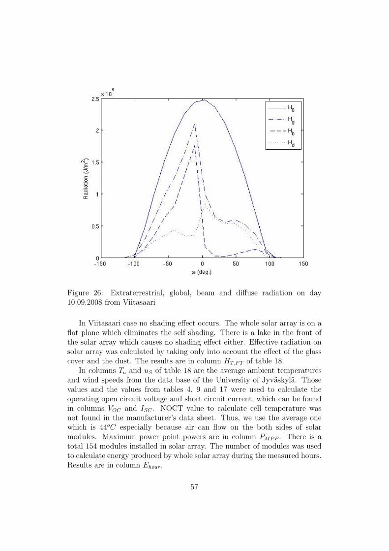
Figure 26: Extraterrestrial, global, beam and diffuse radiation on day10.09.2008 from Viitasaari

In Viitasaari case no shading effect occurs. The whole solar array is on aflat plane which eliminates the self shading. There is a lake in the front ofthe solar array which causes no shading effect either. Effective radiation onsolar array was calculated by taking only into account the effect of the glasscover and the dust. The results are in column HT,FT of table 18.

In columns Ta and uS of table 18 are the average ambient temperaturesand wind speeds from the data base of the University of Jyvaskyla. Thosevalues and the values from tables 4, 9 and 17 were used to calculate theoperating open circuit voltage and short circuit current, which can be foundin columns VOC and ISC . NOCT value to calculate cell temperature wasnot found in the manufacturer’s data sheet. Thus, we use the average onewhich is 44oC especially because air can flow on the both sides of solarmodules. Maximum power point powers are in column PMPP . There is atotal 154 modules installed in solar array. The number of modules was usedto calculate energy produced by whole solar array during the measured hours.Results are in column Ehour.

57

Table 17: Radiation components on tilted surface (β = 5o and γ = 0) andrelative transmittance for beam and circumsolar diffuse radiation componentsfor Viitasaari at 10.09.2008. H:s are in kJ/m2

TO HT,b HT,iso HT,cs HT,hz HT,r HT FTb

0 0 0 0 0 0 0 01 0 0 0 0 0 0 02 0 0 0 0 0 0 03 0 0 0 0 0 0 04 0 0 0 0 0 0 05 0 0 0 0 0 0 06 0.0 38.8 0.0 -0.4 0.0 38.5 0.0007 150.2 97.0 23.6 1.6 0.1 272.4 0.3038 383.9 188.8 80.7 2.5 0.2 656.1 0.5879 712.9 226.1 130.4 5.2 0.4 1074.9 0.74810 929.4 274.9 181.0 4.7 0.5 1390.6 0.83611 1489.3 192.9 166.7 7.0 0.6 1856.6 0.88212 2011.0 188.2 182.0 7.3 0.8 2389.2 0.90313 189.3 663.5 193.7 -2.0 0.4 1045.0 0.90714 25.1 566.5 55.8 -3.5 0.2 644.2 0.89415 19.4 495.6 43.5 -3.1 0.2 555.7 0.86016 61.9 453.4 99.3 -1.6 0.2 613.2 0.79417 103.3 329.3 102.7 0.0 0.2 535.5 0.67118 144.7 174.4 56.4 1.5 0.1 377.2 0.45019 67.4 14.1 1.0 0.6 0.0 83.0 0.06720 0.0 2.9 0.0 0.0 0.0 2.9 0.00021 0 0 0 0 0 0 022 0 0 0 0 0 0 023 0 0 0 0 0 0 0

Sum of the energies of all hours during the years 2006-2008 is E2006−2008(β =5, γ = 0) = 38.08 GJ .

By doing the calculations with different tilt angles in range of β = [0, 90]and with different orientation angles in range of γ = [−90, 90] we receiveE2006−2008(β, γ) and the result can be seen in figure 27. The highest energycan be received with tilt angle β = 46.4o and orientation angle γ = −4.3o

and that is E2006−2008(β = 46.4, γ = −4.3) = 47.76 GJ .

58

Table 18: Effective radiation on tilted surface and photovoltaic generationfrom Viitasaari at 10.09.2008 when β = 5o and γ = 0. HT,FT is in kJ/m2,Ta is in oC, uS is in m/s, VOC is in V , ISC is in A, PMPP is in W and Ehour

is in kJ .TO HT,FT Ta uS VOC ISC PMPP Ehour

0 0 8.12 4.29 0 0 0 01 0 7.72 4.37 0 0 0 02 0 7.16 4.07 0 0 0 03 0 7.07 4.16 0 0 0 04 0 6.82 4.07 0 0 0 05 0 6.59 3.82 0 0 0 06 32 6.32 4.09 5.5 0.03 0.1 307 129 6.23 4.85 28.9 0.03 0.7 4018 407 6.66 4.93 41.7 0.11 3.7 20689 768 7.61 4.64 46.0 0.21 7.7 428610 1082 8.76 3.88 47.3 0.30 11.0 608511 1505 9.68 5.47 48.2 0.42 14.9 827112 1980 10.40 5.77 48.3 0.54 18.3 1014413 866 10.26 5.31 46.2 0.26 9.3 516014 533 10.37 4.62 43.3 0.17 5.9 329415 458 10.32 4.49 42.2 0.15 5.0 277016 491 10.38 3.90 42.7 0.15 5.1 282317 399 10.41 4.54 41.0 0.12 3.8 209418 227 9.84 5.09 35.6 0.06 1.7 95219 16 9.08 5.25 0.0 0.00 0.0 020 2 7.94 4.69 0.0 0.00 0.0 021 0 7.47 3.71 0 0 0 022 0 7.52 3.46 0 0 0 023 0 7.35 3.30 0 0 0 0

9 Discussion

Energy produced The whole solar array at Viitasaari produced 18.18 GJof energy during the years 2006-2008. That was measured by the inventersystem. The measured value is dramatically lower than our estimated valueE2006−2008(β = 5, γ = 0) = 38.08 GJ . According to Ref. [13] one of thereasons for causing this difference is the oversized inverter system. Besides,the inventer efficiency was not calculated in this thesis. However, we believethat the biggest reason for the poor energy production might be that thesolar array had not been serviced at all. Six modules have cracked during its

59

Figure 27: Function of E2006−2008(β, γ) for Viitasaari

operation time. One cracked module in the series of modules will destroy thewhole series power output. Delayed correction has probably been reducingthe total energy produced. Also cracked modules have not been replacedbut they have been connected out from series. That naturally reduces thenumber of modules in whole solar array.

Still, the biggest service issue might be the snow. Typically snow meltsand glides away off the solar module when solar radiation warms up the darksurface of solar module. This solar array is transparent and lowly tilted, andboth of these characteristics lower the melting and gliding effect. In additionthere has been no effort to remove the snow from solar array.

Nowadays Pitajanmaki solar power plant is functional. Actual size of solarpower plant is slightly bigger than the one estimated in this work. Reference[17] reported that in Pitajanmaki power plant there are 870 collector in arrayso that rated power is 181 kWp. Approximate energy production per year

60

was reported to be 160 000kWh which is 1.728 TJ for three years. Powerplant size in this thesis was estimated to be 700 collectors with rated power of140 kWp. Our estimation for the three years energy production with optimaltilt angle was 1.489 TJ .

Tilt and orientation angle Typically optimum tilt angle was informed tobe Latitude ± 10o or from Latitude to Latitude − 10o in many references forexample like in ref. [3] and [5]. According to this information the optimumtilt angle for Pitajanmaki would be 60o or 50o and for Viitasaari 63o or 53o.Both are higher that the estimated ones in this work.

The most sophisticated way to estimate optimum tilt angle for fitted solarcollector was found from [4]. They present function

βopt = 3.7 + 0.69φ (77)

This function has been received by estimating optimum tilt angles for solarcollectors for various geographical locations and creating curve-fitting as afunction of φ. The function will give optimum tilt angle for Pitajanmaki asβopt = 3.7 + 0.69 ∗ 60.12o ≈ 45o and for Viitasaari as βopt = 3.7 + 0.69 ∗63.07o ≈ 47o. In this work the estimated optimum tilt angle for Pitajanmakiis βopt = 28.6o and for Viitasaari is βopt = 46.4o.

In case Pitajanmaki there was shading occurring and in case Viitasaarithere was not. Thus it seems like equation 77 gives a good approximationabout optimum tilt angle when shading effect is not involved. When shadingeffect is involved then equation 77 is more or less useless.

Accuracy of equation 77 is only two digits. For this reason it might be agood tool for estimating optimum tilt angle for household scale installations.For power plant scale installations, which was the case in Pitajanmaki, moreprecise and detailed estimations like one presented in this work are required.

In both cases of Pitajanmaki and Viitasaari maximum energy producingtilt angles βopt = 28.6o and βopt = 46.4o are lower than local latitudes φ =60.12o and φ = 63.07o. This is because more isotropic diffuse irradiation canbe received on surface with lower tilt angle. On the other hand, lowering thetilt angle from latitude angle reduces beam irradiation, circumsolar diffuseirradiation, horizontal diffuse irradiation and ground reflected irradiation onsurface. Because of that 0 < βopt < φ.

Maximum energy producing tilt angle for Pitajanmaki is much smallerthan maximum energy producing tilt angle for Viitasaari even when there isno significant difference between latitudes. This is due to the shading effectwhich occurs at Pitajanmaki. The higher the tilt angle of the rows of solarmodules the higher the effect of shading they cause on each other. This can

61

be also noted when comparing shapes of the curvatures from figures 24 and27. In case of figure 24 a strong reduction of total energy output can benoted when β > 28.6o. Actually, in the case of row installation, it seems thatrows that are not tilted give reasonable energy output. That is E(β = 0, γ)in figure 24. Still it is not reasonable to leave solar collectors without tiltingbecause tilting the solar collector to the right tilt angle gives higher energyoutput and reduces problems with dirt and snow.

The orientation that gives the maximum energy is towards the south inPitajanmaki case and slightly from south to east in Viitasaari case. Eastis the direction where the sun rises up. Thus, the negative γ favors themorning radiation more than the noon radiation. The reason for that canbe understood easily when we examine the measured global radiation datafrom Viitasaari. The total global radiation during the years 2006-2008 atViitasaari was 8.338 GJ/m2. Total 4.248 GJ/m2 of that was radiated atsolar morning (ω < 0) and 4.091 GJ/m2 was radiated at solar noon (ω > 0).

Effect of over-tilting Effect of over tilting is illustrated in figure 28. Over-tilting the solar collector can get slightly higher radiation yields for wintermonths. The price for over-tilting is the strong reduction of total radiationyield due to the reduction of yields of high irradiation summer months. Thus,it is a decision of solar array builders whether they try to make annual energyyield distribution smoother at the expense of total yield reduction. Doingsmoother annual energy yield distribution could be reasonable in the caseof solar heat collectors but probably not in the case of grid connected PV-systems.

How different components of this work have effect on optimum tiltangle In Pitajanmaki case if we investigate what would be the optimum tiltangle taking account only the radiation on tilted surface then βopt = 43.3o.This result has been received using theories from section 4 and finding out thetilt angle that causes the highest radiation on tilted surface. When shadingtheories from section 5 are added to previous we receive βopt = 28.1o. Withthis tilt angle the highest radiation will be received on surface when it isshaded in such a way that is described in section 1. If the effect of glasscover and dust theories from section 6 are added with all the previous thenβopt = 30.9o. And finally when Photovoltaic generation from section 7 istaken account we receive the final result about optimum tilt angle and thatis βopt = 28.6o.

So what is happening? Using only radiation the result is βopt = 43.3o.This is pretty reasonable in many ways. All the narrow theories like equation

62

Figure 28: Effect of over-tilting. Left/lighter bars describe average monthlyeffective radiation distribution in case of Viitasaari when β = βopt = 46.4o

and γ = γopt = −4.3o, right/darker bars describe average monthly effectiveradiation distribution in case of Viitasaari when β = 80.0o and γ = γopt =−4.3o

77 are predicting something like this.When shading effect is included the result changes dramatically to βopt =

28.1o. The result is much lower optimum tilt angle. Reason for this is thathigher tilt angle in rows causes higher shading effect. Because of this theshading effect theory favors lower tilt angles like βopt = 28.1o.

When the effect of glass cover and dust has been taken account thenthe result rises again (βopt = 30.9o). Glass is the most transparent for illu-mination when the illumination meets the glass with low inclination angle.Averagely inclination angles are lowest when solar collector is tilted to lati-tude. In Pitajanmaki case that is 60.12o. For this reason the Effect of glasscover and dust theory change the optimum tilt angle a slightly towards tolatitude value.

When photovoltaic generation has been taken into account then optimumtilt angle value drops again (βopt = 28.6o). This can be explained with the fact

63

that how solar cell responds on different irradiation levels. Solar cell operatespoorly when irradiation level is below 200W/m2. During the morning andlate noon this sort of irradiation level is more common than in middle of theday. On the other hand collectors that are tilted with high tilt angle receivebetter morning and late noon irradiation and collectors which are tilted withlow tilt angle receive better high level middle day irradiation.

64

10 Conclusions

Radiation mostly defines the final yield of solar array. If there is no radiationthere is no yield and if there is a lot of radiation then a big yield is available.Thus, we expect that calculations about radiation on tilted surface plays thebiggest role in our estimation. This is why the most accurate calculationmethod available today to calculate radiation on tilted surface was chosen tobe used here. The method used here is the Perez model that splits radiationin five components and is based on anisotropic sky assumption.

In tentative calculations that were done for Sunwind Gylling Oy beforethis thesis work, the biggest yearly radiation on tilted surface producing tiltangle β was calculated using isotropic sky assumption, equation 25 and dataof year 2009 from Helsinki Kumpula. The shading effect was assumed tobe shading effect for solar collector (not PV-system). The highest energyproducing tilt angle was βopt = 15.0o when orientation was chosen to beγ = 20.

Isotropic sky assumption overestimates the isotropic diffuse radiationcomponent because it assumes all diffuse radiation to be isotropic. Isotropicdiffuse radiates equally from all over the skydome, and therefore it favors thesurfaces with low tilt angles like βopt = 15.0o. Perez model reduces the weightof isotropic diffuse and spreads it more reasonably between three differentdiffuse radiation components. The result is higher maximum energy yieldproducing tilt angle like βopt = 28.6o.

Shading effect needs to be taken into consideration if it occurs. Prooffor that is two dramatically deviating optimum tilt angles from HelsinkiPitajanmaki (βopt = 28.6o) and from Viitasaari (βopt = 46.4o). Effect ofshading limits the directions where radiation is coming from, thus the es-timations were done taking account only the available radiation at shadedcircumstances.

Almost all solar collectors are covered by glass or by materials that be-have like glass under illumination. Taking into account every collector’s glasscover characteristics is complex. We believe that the method used here whichreduces radiation with high inclination angles is proper in all cases. It de-scribes well the typical characteristics of angle dependent transparency ofglass that is covered by dust. The effect of the method to the final result isthat it favors the tilt and orientation angles which give the low inclinationangles to the high radiation hours.

In case of PV-systems the electrical behavior of solar cell is taken into

65

account. That is because PV-system is not functional at extremely low ir-radiation conditions, and on the other hand it gives some estimation aboutyield of planned solar array. One ideal diode model, was used in our calcu-lations because we wanted to do calculations using the data only describedtypically in manufacturers data. One ideal diode model overestimates thepower produced by solar cell [4]. That should be taken into account whenconsidering our results about final yields for solar arrays. Calculating maxi-mum energy producing tilt and orientation angle, the energy production levelhas no effect because its a relative (less solar modules in a system causes lessproduced energy, but it has no effect on βopt and γopt). The electrical charac-teristics of solar cell have effect on βopt and γopt because it stresses radiationhours and radiation components that lead to the greatest energy productionand does not stress low irradiation level conditions when PV-system is hardlyfunctional at all. One ideal diode model takes into account the typical elec-trical characteristics of solar cell, especially when we consider the behavior ofshort circuit current and open circuit voltage under real operation conditions.

The measurement data for the three years was used in both cases ofPitajanmaki and Viitasaari. To calculate the maximum energy producingtilt and orientation angles, the three year measurement data produces areasonable approximation about radiation and weather conditions comparedto average. Although, its an undeniable fact that more years would givebetter approximation. Those three years were sectioned in hours and allhours were separately examined as follows: how much radiation would occuron a tilted surface, how much radiation would be lost caused by shading,how much radiation would go through dirt cover and glass, and finally howmuch energy would the PV-system produce from that radiation in existingweather conditions. Thus, we believe that our method is adequately accurateto calculate an βopt and γopt for any solar array.

References

[1] J. A. Duffie, W. A. Beckham, Solar energy thermal processes, New York:John Wiley & Sons Inc, 1974.

[2] A. B. Meinel, M. P. Meinel, Applied solar energy, an introduction,Addison-Wesley Publishing Company inc, 1976.

[3] J. A Duffie, W. A. Beckham, Solar engineering of thermal processes, 2nded., New York: John Wiley & Sons Inc, 1991.

66

[4] A. Luque, S. Hegedus, Handbook of photovoltaic science and engineering,N.J.: John Wiley & Sons Ltd, 2003.

[5] A. Goetzberger, V. U. Hoffmann, Photovoltaic Solar Energy Generation,Berlin: Springer-Verlag, 2005.

[6] V. Quaschning, Understanding renewable energy systems, London: CarlHanser Verlag GmbG & Co KG, 2005.

[7] S. R. Wenham et al., Applied Photovoltaics, London: Earthscan Publi-cations, 2006.

[8] R. Perez et al., ”Modeling daylight availability and irradiance com-ponents from direct and global irradiance,” Solar Energy, Vol. 44,No. 5, pp. 271-289, 1990. [Online]. Available: ScienceDirect, http:

\\www.sciencedirect.com. [Accessed: March 13, 2010].

[9] L. Stamenic, E. Smiley, K. Karim, ”Low light conditions modeling forbuilding integrated photovoltaic (BIPV) systems,” Solar Energy, Vol.77, pp. 37–45, April 2004. [Online]. Available: ScienceDirect, http:

\\www.sciencedirect.com. [Accessed: March 19, 2010].

[10] D. G. Erbs, S. A. Klein, J. A. Duffie, ”Estimation of the diffuse radiationfraction for hourly, daily and monthly-average global radiation,” SolarEnergy, Vol. 28, No. 4, pp. 293-302, 1982. [Online]. Available: GoogleScholar, http://scholar.google.fi. [Accessed: March 15, 2011].

[11] N. Martin, J. M. Ruzi, ”Calculation of the PV modules angular lossesunder field conditions by means of an analytical model,” Solar EnergyMaterials & Solar Cells, Vol. 70, pp. 25-38, December 2001. [Online].Available: ScienceDirect, http:\\www.sciencedirect.com. [Accessed:March 15, 2011].

[12] N. Martin, J. M. Ruiz, ”A New Method for the Spectral Characterisationof PV Modules,” Progress in Photovoltaics: Research and ApplicationsVol. 7, No 4, pp. 299-310, January 1999. [Online]. Available: WileyOnline Library, http://onlinelibrary.wiley.com. [Accessed: Dec 20,2011].

[13] D. Yang, ”Performance Analysis of a Grid Connected Hybrid Photo-volatic and Wind Electricity Generation System in Cold Climate,” Mas-ter’s Thesis, University of Jyvaskyla, Jyvaskyla, 2007.

67

[14] ”Talvisaan tilastoja,” Finnish Meteorological Institute. [Online]. Avail-able: http://ilmatieteenlaitos.fi/talvitilastot. [Accessed:April 8, 2010].

[15] ”MATLAB - The Language Of Technical Computing,” MathWorks. [On-line]. Available: http://www.mathworks.com/products/matlab. [Ac-cessed: April 17, 2010].

[16] ”Southwest energy efficiency project,” SWEEP. [Online]. Available:http://www.swenergy.org/publications/casestudies/arizona/

tucson\_sesc.htm. [Accessed: Muy 7, 2010].

[17] ”ABB tekee aurinkosahkoa taajuusmuuttajatehtaan kayttoon,”Teknologia Teollisuus, Aug. 25, 2010, [Online]. Available:http://www.teknologiateollisuus.fi. [Accessed: Dec. 20, 2011].

[18] E. Smiley, L. Stamenic, J. Jones, M. Stojanovic, Sixteenth EuropeanPhotovoltaic Solar Energy Conference, pp. 2002-2004, 2000.

[19] L. King, J. Kratochvil, E. Boyson, W. Bower, 2nd World Conference onPhotovoltaic Solar Energy Conversion, pp. 1947-1952, 1998.

68

Nomenclature

Symbol NameAM Air mass [unitless]Hb Beam radiation [J/m2]Hd Diffuse radiation [J/m2]Hg Global radiation [J/m2]HT Radiation on tilted surface [J/m2]ISC Short circuit current [A]IMPP Maximum power point current [A]LH Longitude of local timezone [deg.]LL Local longitude [deg.]NOCT Normal operating cell temperature [Celsius deg.]VOC Open circuit voltage [V]VMPP Maximum power point voltage [V]m Diode factor [unitless]n Number of day of the year [unitless]∆ Atmospheric brightness [unitless]αI Temperature coefficient for current [1/K]αp Profile angle [deg.]αs Solar altitude angle [deg.]αV Temperature coefficient for voltage [1/K]β Tilt angle of solar collector [deg.]γ Surface orientation angle [deg.]γs Solar azimuth angle [deg.]δ Declination [deg.]ε Clearness [unitless]θ The angle of incidence on tilted surface [deg.]θz Zenith angle [deg.]ρ Ground reflectance [unitless]φ Local latitude [deg.]ω Hour angle [deg.]ω1 Starting time of measured hour [deg.]ω2 Ending time of measured hour [deg.]

1

Top SwediSh QualiTySwedish technology you can trust is one of the cornerstones

in Gällivare PhotoVoltaic’s philosophy. The SwedModule

product range is produced using only high quality raw

materials from leading suppliers. The SwedModule is ideal for

individual houses or buildings, on facades or rooftops but also

for large scale solar power systems.

deSign of The SwedModule

The cells are encased in high transmission low-iron tempered

glass, multi-layers of ethylene vinyl acetate (EVA) as well

as Tedlar film. This provides the modules with top-quality

protection against external environmental effects. GPV’s Solar

Power Modules also have bypass diodes to minimise power

loss in case of shading and protect against hot spot effect.

QualiTy ConTrol

During the production process the modules pass through

several quality control check points and they are carefully

checked and tested prior to delivery. The final test takes place

in a solar simulator, where the modules are tested under

Standard Test Conditions (STC 1000W/m²). Every modules

serial number and its test data are stored in our database.

SwedModule gpV200-gpV230Polycrystalline Solar Power Modules

fleXiBiliTyWe have the advantage to have a flexible production facility

where we strive to meet our customer’s needs. Choose from

white, black or transparent tedlar. Silver or black frame or no

frame at all. Please contact us for more information and ask

for a quotation for a product especially designed for you.

warranTy

GPV offer a product guarantee of 10 years

and a 25 year performance guarantee for

an 80 % power output on all standard

products.

In order to further guarantee the quality of

our products we are certified in accordance

with:

• EN IEC 61215

(design qualification and type approval)

• EN IEC 61730 (safety qualification)

• IEC 61701 (salt mist corrosion test)

• SS-EN ISO 9001:2000 (Quality Management System)

• SS-EN ISO 14001:2004

(Environmental Management System)

We connect you to the sun

SwedModule’s on Linköping’s public library. The system is installed by Switchpower.

TEDLAr

TEMPErED GLASS

EVA (EThyLENE VINyL ACETATE)

SOLAr CELLS

EVA

SwedModule gpV200-gpV230Polycrystalline Solar Power Modules

power SpeCifiCaTionSPerformance under standard test conditions

1000 W/m², 25°C, 1.5 AM

GPV200 GPV205 GPV210 GPV215 GPV220 GPV225 GPV230

Average max. power (Pmax) 203.3 Wp 207.2 Wp 212.6 Wp 217.4 Wp 222.7 Wp 226.2 Wp 233.5 Wp

Open circuit voltage (Voc) 36.6 V 36.6 V 36.7 V 36.8 V 36.8 V 36.8 V 36.8 V

Max. power voltage (Vmpp) 29.0 V 29.1 V 29.2 V 29.3 V 29.3 V 29.3 V 29.3 V

Short circuit current (Isc) 7.58 A 7.67 A 7.84 A 7.97 A 8.13 A 8.25 A 8.51 A

Max. power current (Impp) 7.01 A 7.12 A 7.28 A 7.42 A 7.60 A 7.72 A 7.97 A

Gällivare PhotoVoltaic AB Företagscentrum, Box 840, SE-982 28 Gällivare, SwedenT +46 970 158 30 F +46 970 158 98 info@gpv-solar.com www.gpv-solar.com

GPV - A MEMBER OF THE BOREVIND GROUP

phySiCal SpeCifiCaTionS Cell type Polycrystalline

Cell dimension (+/- 0,5mm) 156mm x 156mm

Cells per module 60

Module weight 22 kg

Module size (+/- 2mm) (L x h x W) 1675 mm x 1001 mm x 34 mm

Frame Anodized aluminium

Performance at 800W/m², NOCT, AM1.5

GPV200 GPV205 GPV210 GPV215 GPV220 GPV225 GPV230

Average max. power (Pmax) 145.4 Wp 148.1 Wp 152.0 Wp 155.4 Wp 159.2 Wp 161.7 Wp 166.9 Wp

Open circuit voltage (Voc) 33.1 V 33.1 V 33.2 V 33.3 V 33.3 V 33.3 V 33.3 V

Max. power voltage (Vmpp) 26.0 V 26.1 V 26.2 V 26.3 V 26.3 V 26.3 V 26.3 V

Short circuit current (Isc) 6.26 A 6.34 A 6.48 A 6.59 A 6.72 A 6.82 A 7.03 A

Max. power current (Impp) 5.59 A 5.68 A 5.81 A 5.92 A 6.06 A 6.16 A 6.36 A

All values with a tolerance of ±3 %

Minor reduction in efficiency under partial load conditions at 25°C: at 200W/m², 95% (± 3 %) of the STC efficiency

(1000 W/m²) is achieved.TherMal CharaCTeriSTiCS NOCT 46°C

TC Isc 0.034 %/K

TC Voc -0.34 %/K

SySTeM inTegraTion paraMeTerS

Maximum system voltage: SC II 1000 VDC

Maximum reverse current: Do not apply external voltages

larger than VOC to the module

Gällivare PhotoVoltaic AB reserves the right to make specification changes without prior notice. Please contact your nearest stockist/distributor or visit our website to obtain the latest specification sheet.

ConSTruCTion fronT To BaCk

Module efficiency 12,1 % 12,4 % 12,7 % 13,0 % 13,3 % 13,5 % 13,9 %

ASI THRU® thin-filmsolar module, semitransparent

ASITRHU-30-SG solar modules are designed on the basis of silicium thin-film technology as ASI® tandem cells on a glass substrate. The frameless ASI THRU® solar module consists of aglass front pane with ASI® tandem cells, PVB foil and a heat strengthened backing glass. ASI THRU® solar modules demonstrably produce maximum energy yields. ASI THRU® solar modules combine the features of solar electricity generation, shadowing glare reduction, transparency and soundglass construction in a single element.

ASITHRU-30-SG

New solar architecture: brilliant, colorless transparency

Lateral mounting clearance fromthe connection button

Frameless ASIOPAK-30-SG modules are ideally suited forinstallation in standard facades and roof profile systems.

The structural characteristics of the glass module meetnearly all of the installation requirements specified inDIN 1055. In order to ensure compliance with guide-lines for overhead glass construction, PVB is used as alaminating foil. A general approval for use in overheadglass construction has been issued by the Deutsches Institut für Bautechnik (DIBt-the German Institute of Architectural Engineering).

The modules are factory equipped with plug connectorsand can be connected quickly and safely in series. The specific characteristics of ASI THRU® solar moduleseliminate the need for bypass diodes.

Module type key:SG = laminated safety glass

MC®-plug connectors

ASITHRU-30-SG semitransparent 36 VDC

16 mm

22 mm

• More energy

• General approval for use in overhead

glass construction

• Favorable price per units of surface area

• Multi-purpose module

Current/voltage characteristics at different solar irradiation levels and module temperatures.

MA

NA

GM

ENT

SYST

EMC

ertif

ied

by D

QS

acco

rdin

g to

DIN

EN

ISO

900

1:20

00 ·

Reg

.-N

o. 2

184

DIN

EN

ISO

140

01:1

996

· Re

g.-N

o. 2

184

© 2

003

RWE

SCH

OTT

Sola

r G

mbH

Prin

ted

in t

he F

eder

al R

epub

lic o

f G

erm

any

TM 7

5009

-03

RWE SCHOTT Solar GmbHHermann-Oberth-Str. 1185640 Putzbrunn, GermanyP +49 (0)89 /46264 -100F +49 (0)89 /46264 -111E phototronics-sales@rweschottsolar.comI www.rweschottsolar.com

1000 Wm2, 25 ° C770 Wm2, 70 ° C

750 Wm2, 25 ° C

500 Wm2, 25 ° C

300 Wm2, 25 ° C

0.8

0.6

0.4

0.2

0

1.0

1 0 2 0 3 0 4 0 U[V]

I[A] 36 VDC semitransparent

Electrical data

Initial nominal power 33 Wp

Nominal power* Pnom 27 Wp

Voltage at maximum-power point* Umpp 36 V

Current at maximum-power point* Impp 0.75 A

Short-circuit current* Isc 1.02 A

Open-circuit voltage* Uoc 49 V

Referred to nominal power TK (Pn) - 0.2 % / K

Referred to open-circuit voltage TK (Uoc) - 0.33 % / K

Referred to short-circuit current TK (Isc) + 0.08 % / K

The temperature dependence of the power output is particularly low for ASI THRU®-solar modules.

Maximum system voltage 1000 VDC

Temperature arrange - 40 °C... + 85 °C

Maximum surface load • two-sided clamping along length: 3200 N/m2

• four-sided clamping: 4600 N/m2

Dimensions 1000 x 600 mm2

Module glass thickness / module thickness with connection button 10 mm / 22 mm

Four-sided non-photoactive margin for clamp mounting 16 mm

Weight 14 kg

Dimensions and weights

Cell temperature coefficients

Limits

Characteristic data

The quoted figures are subject to a production tolerance of ± 10%.* These data represent stabilized electrical module performance at standart test conditions (STC – 1000 W/m2, spectrum AM 1.5,

25 °C cell temperature). The nominal power may be initially approx. 18% higher than the quoted stabilized power data.

Specifications subject to change without notice.

IEC 61646 certified

Qualification CE conformity

Safety Class II

Solar cell type thin-film amorphous silicon in ASI® tandem cells

Appearance uniformly dark-brown

Semitransparency about 10 % transmission, colour-neutral

Electrical connection double insulated cable (Huber & Suhner), 2.5 mm2 cross-section,

100 cm length per polarity, MC®-plug connectors