Effects Of Gaze-Contingent Stimuli On Eye...
100
Effects Of Gaze-Contingent Stimuli On Eye Movements Diplomarbeit Michael Dorr Ausgegeben von Prof. Dr. rer. nat. Thomas Martinetz Betreut von Dr.-Ing. Erhardt Barth Institut f¨ ur Neuro- und Bioinformatik Universit¨ at zu L ¨ ubeck L¨ ubeck, Deutschland 2004 (Eingereicht 02.04.2004)
Transcript of Effects Of Gaze-Contingent Stimuli On Eye...

Effects Of Gaze-Contingent Stimuli On Eye Movements
Diplomarbeit
Michael Dorr
Ausgegeben von
Prof. Dr. rer. nat. Thomas Martinetz
Betreut von
Dr.-Ing. Erhardt BarthInstitut fur Neuro- und Bioinformatik
Universitat zu Lubeck
Lubeck, Deutschland
2004
(Eingereicht 02.04.2004)

ii
© 2004
Michael Dorr
All Rights Reserved

Statement of Originality
The work presented in this thesis is, to the best of my knowledge and belief, original,
except as acknowledged in the text. The material has not been submitted, either in whole
or in part, for a degree at this or any other university.
Ich versichere an Eides statt durch meine Unterschrift, dass ich die vorliegende Arbeit
selbstandig und ohne fremde Hilfe angefertigt und alle Stellen, die ich wortlich oder an-
nahernd wortlich aus Veroffentlichungen entnommen habe, als solche kenntlich gemacht
habe, mich auch keiner anderen als der angegebenen Literatur oder sonstiger Hilfsmit-
tel bedient habe. Die Arbeit hat in dieser oder ahnlicher Form noch keiner anderen
Prufungsbehorde vorgelegen.
Lubeck, 02.04.2004
Abstract
Although we are mostly unaware of the fact that our eyes move several times per second,
the way we perceive the world depends to a large extent on the exact scan paths our eyes
describe. Indeed, recent studies have impressively shown that even substantial changes to
a visual display can go unnoticed if the observer’s attention is directed somewhere else.
Therefore, one of the goals of the Information technology for active perception (Itap)
project is to improve communication systems by guiding the scan path of an observer.
In this thesis, a system was implemented that allows to perform first experiments towards
this goal. This system consists of a workstation that is connected to an eye-tracking
device. High resolution movies can be displayed and manipulated in real time. The
manipulation depends on the structure of the image sequence and on the gaze of the
observer. To reduce the overall latency was a major design goal so that the system is
capable of reacting to an eye movement within less than 30 ms.
Results will be presented for experiments where image sequence manipulations were de-
signed to attract the gaze of an observer. One of these manipulations was the sudden
onset of a red square, the other stimulus type simulated the optical flow of an object
moving towards the observer. The results show that it is possible to influence the gaze
of an observer, but the strength of this effect seems to depend on the underlying image
sequence.

Zusammenfassung
Unsere Augen bewegen sich mehrere Male pro Sekunde, meist ohne dass uns dies bewusst
wird. Tatsachlich aber hangt unsere Wahrnehmung in hohem Maße von den genauen
Mustern unserer Augenbewegungen, den sogenannten scan paths ab. Auch große Ander-
ungen an visuellen Szenen werden oftmals nicht erkannt, wenn die Aufmerksamkeit des
Beobachters nur anderweitig gebunden ist, wie neue Studien eindrucksvoll zeigen. Ein
Ziel des Projekts ”Information technology for active perception” (Itap) ist es daher, den
scan path eines Beobachters zu lenken und damit verbesserte Kommunikationssysteme
zu schaffen.
In Rahmen der vorliegenden Arbeit wurde ein System implementiert, das erste Experi-
mente auf dem Weg zu diesem Ziel erlaubt. Das System besteht aus einer Workstation,
die mit einem Eye-Tracker verbunden wird. Hochauflosende Videosequenzen konnen
damit in Echtzeit angezeigt und manipuliert werden. Die Manipulation hangt dabei von
der orts-zeitlichen Krummung der Videosequenz sowie von der Blickrichtung des Betra-
chters ab. Ein wesentliches Entwurfsziel war eine moglichst geringe Latenz, so dass das
System innerhalb von weniger als 30 ms auf eine Augenbewegung reagieren kann.
Es werden Ergebnisse fur Experimente gezeigt, in denen die Sequenzmanipulationen
dazu dienten, die Blickrichtung des Probanden anzuziehen. Ein verwendeter Stimulus
bestand dabei aus dem abrupten Auftauchen eines roten Objekts, der zweite Stimulustyp
simuliert den optischen Fluss eines Objekts, das sich dem Beobachter nahert. Die Ergeb-
nisse zeigen, dass es zwar moglich ist, die Blickrichtung eines Probanden zu beeinflussen,
die Starke dieses Effekts scheint jedoch von der Videosequenz abzuhangen.

Acknowledgements
Florian Mosch from the Institute for Technical Informatics gave me valuable advice on
how to measure the latency of our experimental setup. Manuel Wille managed to convince
me that mysterious system behaviour is always due to the programmer, so that there is
always hope. Sabine Dorr served as a patient guinea pig during testing. Martin Bohme
wrote the software on which the program to compute the spatio-temporal curvature of
image sequences is based.
This thesis was written in the context of the ModKog project funded by the BMBF (Ger-
man Ministry for Research and Education).

Contents
Statement of Originality iii
Abstract iv
Zusammenfassung v
Acknowledgements vi
1 Introduction 1
2 The Human Visual System 7
2.1 Anatomy . . . . . . . . . . . . . . . . . . . . . . . . . . . . . . . . . 7
2.1.1 Eye . . . . . . . . . . . . . . . . . . . . . . . . . . . . . . . . 7
2.1.2 Retina . . . . . . . . . . . . . . . . . . . . . . . . . . . . . . . 8
2.1.3 Beyond the Retina . . . . . . . . . . . . . . . . . . . . . . . . 11
2.2 Psychophysics . . . . . . . . . . . . . . . . . . . . . . . . . . . . . . . 12
2.3 The Active Vision Paradigm . . . . . . . . . . . . . . . . . . . . . . . 13
2.4 Eye Movements . . . . . . . . . . . . . . . . . . . . . . . . . . . . . . 14
2.4.1 Neural Systems . . . . . . . . . . . . . . . . . . . . . . . . . . 14
2.4.2 Saccades . . . . . . . . . . . . . . . . . . . . . . . . . . . . . 15
2.4.3 Other Types Of Eye Movements . . . . . . . . . . . . . . . . . 20
3 Attention 23
3.1 Spatial Selectivity . . . . . . . . . . . . . . . . . . . . . . . . . . . . . 25
3.2 Limits of Attention . . . . . . . . . . . . . . . . . . . . . . . . . . . . 26
3.3 Attention and Gaze . . . . . . . . . . . . . . . . . . . . . . . . . . . . 26
3.4 Capture of Attention . . . . . . . . . . . . . . . . . . . . . . . . . . . 28
viii
4 Blindnesses 29
4.1 Change Blindness . . . . . . . . . . . . . . . . . . . . . . . . . . . . . 30
4.1.1 Phenomena . . . . . . . . . . . . . . . . . . . . . . . . . . . . 30
4.1.2 Possible Explanations . . . . . . . . . . . . . . . . . . . . . . 32
4.2 Inattentional Blindness . . . . . . . . . . . . . . . . . . . . . . . . . . 33
4.2.1 Possible Explanations . . . . . . . . . . . . . . . . . . . . . . 34
5 Theory 37
5.1 Preliminaries . . . . . . . . . . . . . . . . . . . . . . . . . . . . . . . 37
5.2 Overview . . . . . . . . . . . . . . . . . . . . . . . . . . . . . . . . . 39
5.3 Stimulus Types . . . . . . . . . . . . . . . . . . . . . . . . . . . . . . 39
5.3.1 Red Dot Stimulus . . . . . . . . . . . . . . . . . . . . . . . . . 39
5.3.2 Looming Effect Stimulus . . . . . . . . . . . . . . . . . . . . . 40
5.4 Stimulus Placement . . . . . . . . . . . . . . . . . . . . . . . . . . . . 40
5.5 Stimulus Duration . . . . . . . . . . . . . . . . . . . . . . . . . . . . . 43
5.6 Saccade Detection . . . . . . . . . . . . . . . . . . . . . . . . . . . . . 43
5.7 Data Analysis . . . . . . . . . . . . . . . . . . . . . . . . . . . . . . . 44
6 System Description 47
6.1 Functional Specification . . . . . . . . . . . . . . . . . . . . . . . . . 47
6.2 Hardware . . . . . . . . . . . . . . . . . . . . . . . . . . . . . . . . . 47
6.2.1 Eye Tracker Workstation . . . . . . . . . . . . . . . . . . . . . 47
6.2.2 Display Workstation . . . . . . . . . . . . . . . . . . . . . . . 49
6.3 Software . . . . . . . . . . . . . . . . . . . . . . . . . . . . . . . . . . 50
6.3.1 Calibration . . . . . . . . . . . . . . . . . . . . . . . . . . . . 50
6.3.2 Coordinate System Transformation . . . . . . . . . . . . . . . 51
6.3.3 Timing . . . . . . . . . . . . . . . . . . . . . . . . . . . . . . 51
6.3.4 Classes . . . . . . . . . . . . . . . . . . . . . . . . . . . . . . 53
6.3.5 Data Analysis . . . . . . . . . . . . . . . . . . . . . . . . . . . 54
7 Timing Validation 59
7.1 Theory . . . . . . . . . . . . . . . . . . . . . . . . . . . . . . . . . . . 59
7.2 Measurements . . . . . . . . . . . . . . . . . . . . . . . . . . . . . . . 61

ix
8 Results 65
8.1 Movies . . . . . . . . . . . . . . . . . . . . . . . . . . . . . . . . . . 65
8.2 Results . . . . . . . . . . . . . . . . . . . . . . . . . . . . . . . . . . . 68
8.2.1 Low Saliency Movie . . . . . . . . . . . . . . . . . . . . . . . 69
8.2.2 High Saliency Movie . . . . . . . . . . . . . . . . . . . . . . . 70
8.2.3 Invisible Stimuli As Baseline Reference . . . . . . . . . . . . . 70
8.2.4 High Resolution, Medium Saliency Movie . . . . . . . . . . . . 71
8.3 Remarks . . . . . . . . . . . . . . . . . . . . . . . . . . . . . . . . . . 71
9 Discussion 81
Bibliography 84


C H A P T E R 1
Introduction
We perceive our visual world as colourful and rich in detail across the whole visual field.
The fact that we actually perceive only very little detail at a time remains mainly un-
conscious because we constantly scan the visual world by moving our eyes. These eye
movements are not only a necessary prerequisite for successful visual perception, but
their exact order does also determine to a large extent how we perceive the visual world.
For specific tasks, the human visual system deploys specific patterns of eye movements,
or scan paths. This also means that a given scan path can be unsuitable for unexpected
situations or tasks, for example change detection.
Although there have been many experiments (e.g. [SD00, LG03]) that studied what kind
of stimuli could evoke eye movements, to our knowledge no experiments have been per-
formed to show whether it is possible to alter the scan path of an observer viewing dy-
namic natural scenes.
The goal of this thesis was now to build a prototype system that could affect the eye
movements subjects made while looking at video clips of dynamic natural scenes. To this
end, these video clips would be manipulated dependent on the current fixation point and
the intrinsic dimensionality of the image sequence to create stimuli that were designed to
attract the observers’ gaze.
These experiments hopefully allow to continue towards systems that are able to guide the
scan path of an observer. Such a recommended scan path could improve human-machine
communication, maximize information content of a display, or could function as a help to
disabled people.

2 Introduction
In the following, we will give a short overview about the contents of this thesis. As to
the notation throughout the thesis, specific terminology will be introduced in italics, but
afterwards used without typographical highlighting.
A common intuition as to the nature of visual perception is that somehow light is reflected
from a visual scene and projected into our eyes and towards the brain, where the light
patterns are transformed to some sort of brain representation. In this intuition, ”seeing”
is mainly determined by the physical characteristics of the visual world, by bottom-up
processes.
This intuition is, for example, reflected in the ”traditionalist” approach to modelling vision
in David Marr’s Vision ([Mar82]). In his words, ”to see is to know what is where by
looking”. According to this view, the eye takes a ”snapshot” of the visual scenery which
is then processed in detail in the visual system. First, information about intensity changes
and their geometrical distribution and organization is extracted (the primal sketch). Then,
the orientation and depth of surfaces are made explicit in the 2 1/2-D sketch until finally
a 3-D model representation is formed.
But as we will see in chapter 2, the human eye is not built like a digital camera. While
this analogy might make some sense for the optical part of the eye, the retina is radically
different from a CCD chip. The photoreceptors of the retina are not arranged on a fixed
rectangular grid, but are packed somewhat hexagonally, with the variations in size and
shape that are inevitable in biological systems. Most importantly, though, the distribution
of the different types of retinal cells varies greatly over the retina. Because this is also
true for the cells in later stages of the visual system, visual function needs to be expressed
as a function of eccentricity. For example, spatial acuity has its maximum in the fovea,
the center of the visual field, whereas the periphery is especially sensitive to motion.
To overcome the limits of vision at given points in the visual field, the eyes move about
2-3 times per second. These eye movements are called saccades and go unnoticed most
of the time. This is especially intriguing because during a saccade, the visual scenery
moves across the retina with up to 700°/s, but we still perceive our visual world as stable.
This holds also true for the translations of the retinal image that occur due to head or body
movements.
These observations have led to the Active Vision paradigm. This paradigm states that the

Introduction 3
role of the visual system is not only that of passive perception. Ultimately, the goal of
sensors is to allow, or guide, useful behaviour. Consequently, two kinds of visual pro-
cesses must be distinguished. The focal system is concerned with object recognition and
the extraction of abstract information from a scene, whereas the ambient system guides
spatially oriented behaviour and locomotion ([Bri00]).
This paradigm is supported by the finding that eye movements are highly task-specific
([HBT+02]). One determining factor for the control of eye movements is attention, on
which some work will be presented in chapter 3.
Attention has been described as spatially selective. Only a part of a scene can be attended
to at any given moment, or, by Posner’s metaphor ([Pos80]), illuminated by a ”spotlight”.
This means that there must be a procedure that controls the direction of the spotlight
beam.
Necessarily, there must be some influence of bottom-up processes, which means that at-
tention is modulated by local properties of the sensory input. On the other hand, top-down
processes are also involved. These include knowledge, assumptions, and expectations
about the scene as well as the subject’s state, such as level of alertness.
”The visual system must balance the selectivity of ongoing task specific computations
against the need to remain responsive to novel and unpredictable visual input that may
change the task agenda.” ([HBT+02])
The metaphor of attention as a spotlight naturally leads to the question what happens to
those parts of the world that are not illuminated by the spotlight’s beam at a given instant?
Chapter 4 introduces a phenomenon called change blindness. O’Regan et al. created
movies where significant changes were made to a scene ([ORC00]). The temporal tran-
sient caused by the change was masked by covering the scene with blank squares (hence
the name ”mudsplash movies”). Without the temporal transient to attract attention, many
observers failed to notice the change. This effect can also be evoked with changes made
while the observer performs a saccade or blinks [ODCR00].
But subjects need not be ”blind” against sudden changes only. In a classic and especially
striking example, Simons and Chabris showed a movie of two basketball teams to a group
of subjects ([SC99]). Both teams passed balls back and forth and it was the subjects’ task
to count the number of passes or the number of bounces and passes of one of the teams.
4 Introduction
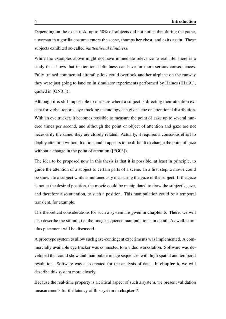
Depending on the exact task, up to 50% of subjects did not notice that during the game,
a woman in a gorilla costume enters the scene, thumps her chest, and exits again. These
subjects exhibited so-called inattentional blindness.
While the examples above might not have immediate relevance to real life, there is a
study that shows that inattentional blindness can have far more serious consequences.
Fully trained commercial aircraft pilots could overlook another airplane on the runway
they were just going to land on in simulator experiments performed by Haines ([Hai91],
quoted in [ON01])!
Although it is still impossible to measure where a subject is directing their attention ex-
cept for verbal reports, eye-tracking technology can give a cue on attentional distribution.
With an eye tracker, it becomes possible to measure the point of gaze up to several hun-
dred times per second, and although the point or object of attention and gaze are not
necessarily the same, they are closely related. Actually, it requires a conscious effort to
deploy attention without fixation, and it appears to be difficult to change the point of gaze
without a change in the point of attention ([FG03]).
The idea to be proposed now in this thesis is that it is possible, at least in principle, to
guide the attention of a subject to certain parts of a scene. In a first step, a movie could
be shown to a subject while simultaneously measuring the gaze of the subject. If the gaze
is not at the desired position, the movie could be manipulated to draw the subject’s gaze,
and therefore also attention, to such a position. This manipulation could be a temporal
transient, for example.
The theoretical considerations for such a system are given in chapter 5. There, we will
also describe the stimuli, i.e. the image sequence manipulations, in detail. As well, stim-
ulus placement will be discussed.
A prototype system to allow such gaze-contingent experiments was implemented. A com-
mercially available eye tracker was connected to a video workstation. Software was de-
veloped that could show and manipulate image sequences with high spatial and temporal
resolution. Software was also created for the analysis of data. In chapter 6, we will
describe this system more closely.
Because the real-time property is a critical aspect of such a system, we present validation
measurements for the latency of this system in chapter 7.

Introduction 5
Some preliminary experiments were also performed. The results for the experiments are
presented in chapter 8. It will be shown that there is indeed an effect of the presented
stimulation on eye movement patterns. Nevertheless, the strength of this effect seems to
depend on the underlying scene that is manipulated as well.
In chapter 9, these results will be discussed. We will also give an outlook to possible
extensions.

C H A P T E R 2
The Human Visual System
2.1 Anatomy
2.1.1 Eye
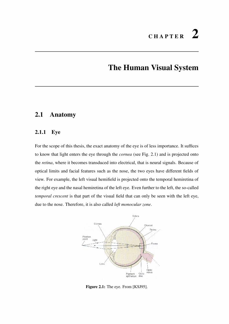
For the scope of this thesis, the exact anatomy of the eye is of less importance. It suffices
to know that light enters the eye through the cornea (see Fig. 2.1) and is projected onto
the retina, where it becomes transduced into electrical, that is neural signals. Because of
optical limits and facial features such as the nose, the two eyes have different fields of
view. For example, the left visual hemifield is projected onto the temporal hemiretina of
the right eye and the nasal hemiretina of the left eye. Even further to the left, the so-called
temporal crescent is that part of the visual field that can only be seen with the left eye,
due to the nose. Therefore, it is also called left monocular zone.
Figure 2.1: The eye. From [KSJ95].

8 The Human Visual System
Figure 2.2: Visual hemifields. From [KSJ95].
The main source of optical imperfections is the shape of the lens which leads to spherical
aberrations, an effect that is stronger towards the periphery.
The eyeball can move in its socket with six degrees of freedom, three each for rotation and
translation. The muscles responsible for these movements are the superior and inferior
recti for up/down movement, the medial and lateral recti for left/right movement, and the
superior and inferior obliques for rotational movement.
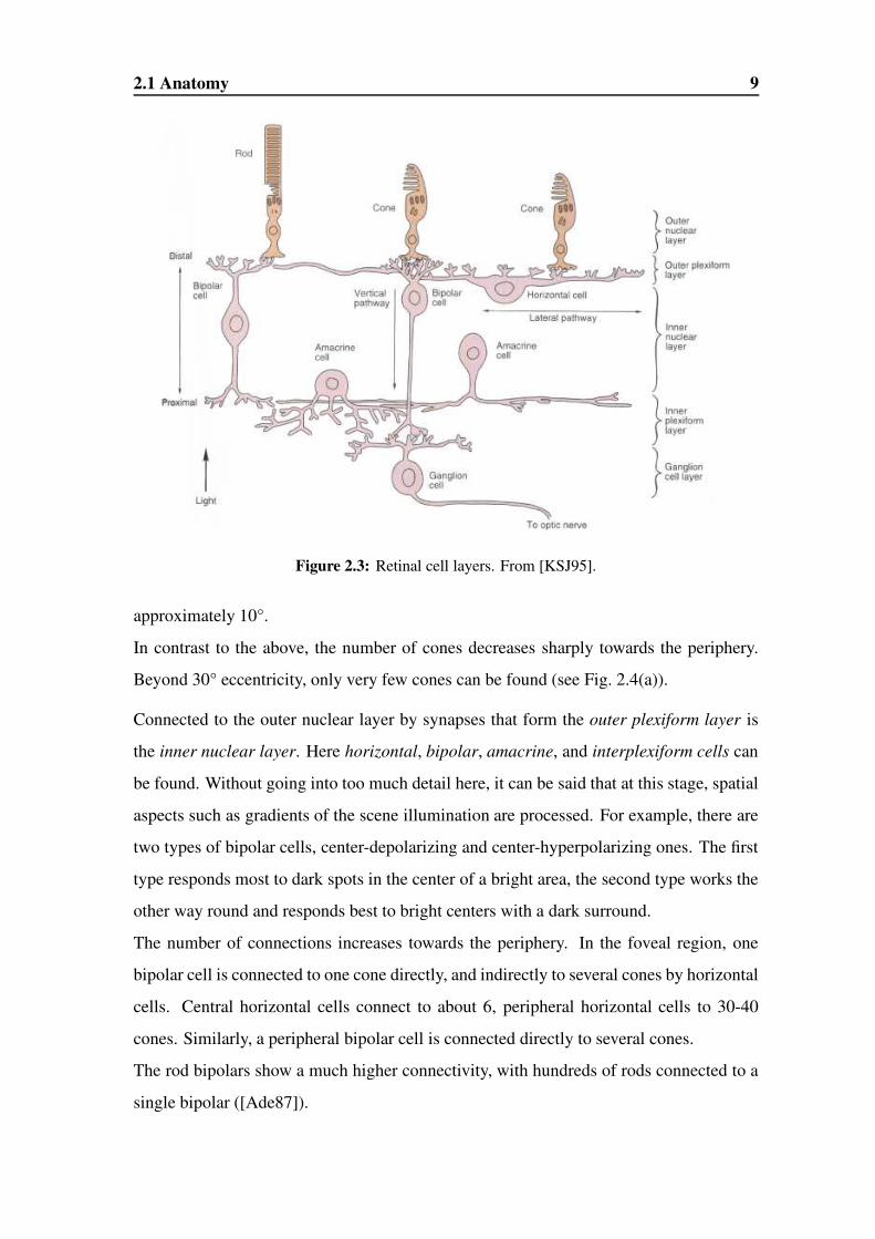
2.1.2 Retina
The retina consists of three different cell layers and, interspersed in-between, two synaptic
layers. Farthest away from the incoming light is the outer nuclear layer that contains the
photoreceptors that convert incoming light to electrical impulses. There are two types of
photoreceptors, rods and cones. Rods are far more numerous than cones with about 120
million rods as opposed to about 7 million cones. Rods also come in just one type that is
responsible for achromatic low-light vision, whereas cones can be separated into S-, M-,
and L-types which are sensitive to short, medium, and long wavelengths, respectively, and
thus allow colour vision. The differences of rods and cones are summarized in Table 2.1.
As can be seen in Fig. 2.4(a), the density of rods and cones varies greatly across the visual
field. The central 2° of the retina are called the fovea which contains only very few rods.
Actually, the central 1° has no rods at all and is called foveola. Because of the macula, a
region of yellow pigmentation over the fovea, foveal vision is also often called macular
vision. The term parafoveal vision is used for the visual field around the fovea spanning
2.1 Anatomy 9
Figure 2.3: Retinal cell layers. From [KSJ95].
approximately 10°.
In contrast to the above, the number of cones decreases sharply towards the periphery.
Beyond 30° eccentricity, only very few cones can be found (see Fig. 2.4(a)).
Connected to the outer nuclear layer by synapses that form the outer plexiform layer is
the inner nuclear layer. Here horizontal, bipolar, amacrine, and interplexiform cells can
be found. Without going into too much detail here, it can be said that at this stage, spatial
aspects such as gradients of the scene illumination are processed. For example, there are
two types of bipolar cells, center-depolarizing and center-hyperpolarizing ones. The first
type responds most to dark spots in the center of a bright area, the second type works the
other way round and responds best to bright centers with a dark surround.
The number of connections increases towards the periphery. In the foveal region, one
bipolar cell is connected to one cone directly, and indirectly to several cones by horizontal
cells. Central horizontal cells connect to about 6, peripheral horizontal cells to 30-40
cones. Similarly, a peripheral bipolar cell is connected directly to several cones.
The rod bipolars show a much higher connectivity, with hundreds of rods connected to a
single bipolar ([Ade87]).

10 The Human Visual System
rods conesnight vision, high sensitivity to light day vision, low sensitivity to lightsingle photon detection detect only hundreds of photonsachromatic three different types: S-, M-, L-cones
(blue, green, red)low spatial resolution high spatial resolutionhighly convergent neural pathways less convergent pathwayslow temporal resolution (12 Hz) high temporal resolution (55 Hz)fixed size across the visual field bigger towards the periphery
Table 2.1: Differences between rods and cones.
Further towards the incoming light lie the inner plexiform layer and, connected by it, the
ganglion cell layer. In order to increase acuity, the ganglion cells in front of the fovea are
shifted sideways towards the periphery so that rays of light hitting the fovea do not get
distorted. The approximately one million ganglion cells can be discriminated morpholog-
ically into two types and functionally into three types. Morphologically, about 80% of
ganglion cells are of the β-type. They have relatively small cell bodies and dendrites, and
their projections go to the parvo-cellular layer of the lateral geniculate nucleus, a brain
area that relays signals to the visual cortex. They are well-suited to the discrimination of
fine details, low contrast, and colour. The α-type cells make up about 10% of the ganglion
cells. They have larger cell bodies and dendrites, are achromatic, and they respond better
to moving stimuli. Their projections go to the magno-cellular layer.
Functionally, X-, Y-, and W-type ganglion cells can be distinguished. X-cells project
to both the parvo- and magno-cellular layers and are sensitive to stationary stimuli with
fine detail. Y-cells, on the other hand, project to the magno-cellular layer only and are
sensitive to transient stimuli or motion.
Of special interest are the W-type ganglion cells. They are sensitive to coarse features
and motion and project to the superior colliculus, a brain area that is concerned with the
control of involuntary eye movements.
In summary, it can be said that at the retinal level already, a great deal of information
processing takes place. This processing is especially concerned with encoding change, be
it spatial or temporal.

2.1 Anatomy 11
(a) (b)
Figure 2.4: Functions of eccentricity: a) Density of rods and cones. b) Visual acuity. From[DV00].
2.1.3 Beyond the Retina
Visual signals from the retina are sent through the optic nerve towards the processing
sites in the brain. On their way, the fibres from both right and left hemifields are brought
together at the optic chiasm (see Fig. 2.5).
The two optic tracts project to three subcortical targets. The lateral geniculate nucleus
relays data to the primary visual cortex at the back of the head. Here, higher-order infor-
mation processing such as form extraction or motion estimation takes place. Conscious
perception is based on these processes. The other two targets are the pretectum that is
responsible for pupillary reflexes, and the superior colliculus that uses its visual input to
generate involuntary eye movements ([KSJ95]).
The optic tracts can be discriminated into two pathways, the parvo- and magno-cellular
pathways. As we have seen before, different types of ganglion cells project to these two
pathways. Due to their cell characteristics and their apparent functional distinction, the
parvo-cellular pathway is also called the what pathway while the magno-cellular path-
way is called the where pathway. The P-pathway is concerned with the details of an
object and object recognition (”what”). It can actually be further discriminated into the
parvocellular-blob pathway and the parvocellular-interblob pathway. The former deals
12 The Human Visual System
with the perception of colour, the latter with the perception of shapes and depth. The
M-pathway is concerned with the spatial relationship of objects and behaviour oriented
towards them (”where”). This distinction cannot only be made on anatomical grounds, but
can also be established with patients who suffered a brain damage, usually due to a stroke,
that left only one of the pathways intact. Despite this distinction, there are interactions
between the pathways at many different levels ([KSJ95]).
In general, information processing at the cortical level is not well understood yet. There
is a multitude of distinguishable areas, but because of their complex interactions, and
because of many open philosophical questions about perception in general, there is no
full explanation for their functioning.
2.2 Psychophysics
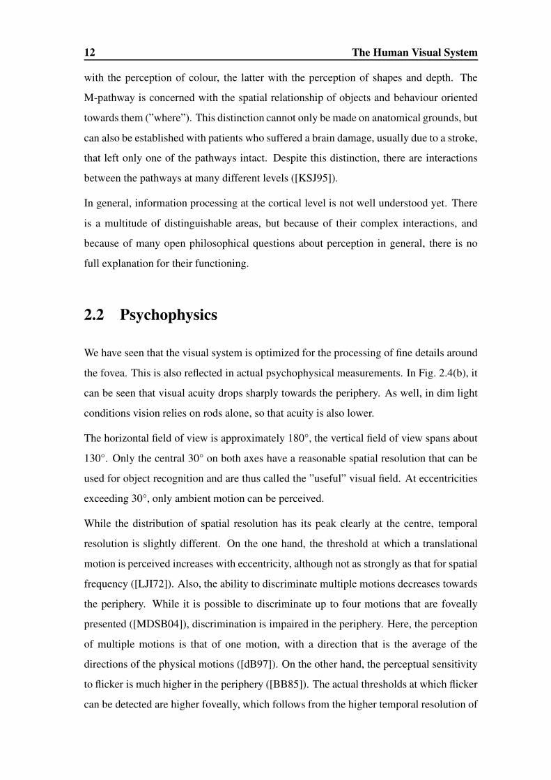
We have seen that the visual system is optimized for the processing of fine details around
the fovea. This is also reflected in actual psychophysical measurements. In Fig. 2.4(b), it
can be seen that visual acuity drops sharply towards the periphery. As well, in dim light
conditions vision relies on rods alone, so that acuity is also lower.
The horizontal field of view is approximately 180°, the vertical field of view spans about
130°. Only the central 30° on both axes have a reasonable spatial resolution that can be
used for object recognition and are thus called the ”useful” visual field. At eccentricities
exceeding 30°, only ambient motion can be perceived.
While the distribution of spatial resolution has its peak clearly at the centre, temporal
resolution is slightly different. On the one hand, the threshold at which a translational
motion is perceived increases with eccentricity, although not as strongly as that for spatial
frequency ([LJI72]). Also, the ability to discriminate multiple motions decreases towards
the periphery. While it is possible to discriminate up to four motions that are foveally
presented ([MDSB04]), discrimination is impaired in the periphery. Here, the perception
of multiple motions is that of one motion, with a direction that is the average of the
directions of the physical motions ([dB97]). On the other hand, the perceptual sensitivity
to flicker is much higher in the periphery ([BB85]). The actual thresholds at which flicker
can be detected are higher foveally, which follows from the higher temporal resolution of
2.3 The Active Vision Paradigm 13
cones. Because this effect is again not as strong as the difference in spatial resolution, the
perceptual salience of flicker in the periphery might be explained by the relative strength
of responses to moving as opposed to stationary stimuli.
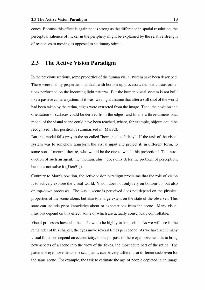
2.3 The Active Vision Paradigm
In the previous sections, some properties of the human visual system have been described.
These were mainly properties that dealt with bottom-up processes, i.e. static transforma-
tions performed on the incoming light patterns. But the human visual system is not built
like a passive camera system. If it was, we might assume that after a still shot of the world
had been taken by the retina, edges were extracted from the image. Then, the position and
orientation of surfaces could be derived from the edges, and finally a three-dimensional
model of the visual scene could have been reached, where, for example, objects could be
recognized. This position is summarized in [Mar82].
But this model falls prey to the so-called ”homunculus fallacy”. If the task of the visual
system was to somehow transform the visual input and project it, in different form, to
some sort of mentral theatre, who would be the one to watch this projection? The intro-
duction of such an agent, the ”homunculus”, does only defer the problem of perception,
but does not solve it ([Den91]).
Contrary to Marr’s position, the active vision paradigm proclaims that the role of vision
is to actively explore the visual world. Vision does not only rely on bottom-up, but also
on top-down processes. The way a scene is perceived does not depend on the physical
properties of the scene alone, but also to a large extent on the state of the observer. This
state can include prior knowledge about or expectations from the scene. Many visual
illusions depend on this effect, some of which are actually consciously controllable.
Visual processes have also been shown to be highly task-specific. As we will see in the
remainder of this chapter, the eyes move several times per second. As we have seen, many
visual functions depend on eccentricity, so the purpose of these eye movements is to bring
new aspects of a scene into the view of the fovea, the most acute part of the retina. The
pattern of eye movements, the scan paths, can be very different for different tasks even for
the same scene. For example, the task to estimate the age of people depicted in an image

14 The Human Visual System
gives rise to different scan paths than the task to describe what they are doing.
2.4 Eye Movements
The first description of jump-like eye movements has been made 1878 by the French
ophthalmologist Javal ([Jav78], as described in [RS04]). In his experiments, he used a
mirror to monitor the eye movements subjects made while reading, so that his analysis
was restricted to qualitative statements.1 The quantitative study of eye movements dates
back to Yarbus 1967 ([Yar67]). He observed that the eyes move about 2-3 times per
second in jump-like movements, the so-called saccades2. 90% of viewing time, on the
other hand, are spent with the eyes apparently stationary, in fixations. These fixations have
a duration of about 150-600 ms ([DV00]). When eye movements are recorded accurately
enough, it turns out that even during fixations, the eyes are not perfectly still. Tremor, for
example, seems to be due to the imperfection of the oculomotor system and causes very
small eye movements with an amplitude of less than one minute of arc. If an image is
artificially stabilized on the retina, its percept actually disappears after around a second,
so these micro-movements might also serve the purpose of preventing the adaptation of
retinal cells.
Of central interest in this thesis will be saccades, that is goal-directed eye movements with
an amplitude of about 0.5-60° and a peak velocity of several hundred degrees per second.
Therefore, we will present some data on them in the following sections. Because the
measurement of eye movements is still error-prone even today, we will also name some
of the problems associated with the study of eye movements.
2.4.1 Neural Systems
Three neural systems can be distinguished that deal with eye movements, see Fig. 2.5.
The superior colliculus controls involuntary eye movements, while the occipital cortex
1The technical difficulties the pioneers in eye movement research faced might be reflected in the quotethat 20 years after Javal, ”[the] plaster of Paris that will attach itself firmly and immovably to any moistsurface” ([Del98], quote from [RS04]) was used to fix a small cap on an eye that transduced horizontal eyemovements onto a rotating drum.
2The French word saccade describes the flick of a ship’s sail when it catches the wind.

2.4 Eye Movements 15
Figure 2.5: Neural systems related to eye movements. From [KSJ95].
accounts for voluntary ones. These two systems are responsible for target-oriented sac-
cades, while the semicircular canals produce reflexive eye movements that compensate
for head or body movement or rotation.
Most models (e.g., [Bec91, RZHB02]) of the control of saccadic eye movements assume
that there are two distinct processes involved that run in parallel. The first process is
a decision process that selects the next visual target from the present visual scene, the
second one computes the motor commands that are actually necessary to execute the
desired eye movement. The existence of these two separate processes can be inferred, for
example, from visual search tasks where reaction times are measured ([BJ79]).
2.4.2 Saccades
Problems
The study of eye movements has to deal with several problems. First of all, the different
technical methods to measure eye movements all have severe drawbacks. An ideal eye
tracker should be fast, accurate, and inobtrusive, but unfortunately these requirements are,

16 The Human Visual System
to some extent, mutually exclusive.
But even when measured with an (hypothetical) optimal technical device, eye movement
data analysis still faces a number of challenges. There are many different control pro-
cesses involved, many of which work in closed loops. For example, saccades are often
not perfectly accurate, so that corrective eye movements are made, but the latency of these
corrections is by no means uniform. The direction in which a visual target lies is also an
important factor, which is not only a problem of the underlying neural systems, but of the
muscular realization of the oculomotor system as well. Additionally, eyeball position and
orientation are complemented by position and orientation of the head, because the head
remains stationary only for relatively small saccades.
Apart from the random variations that might be expected in a biological system, the two
eyes also differ in their movement dynamics, depending on the location of the visual
target.
Amplitude and Duration
By mechanical constraints, the amplitude of (horizontal) eye-in-head movements is lim-
ited to about ± 55° away from the central position. For saccades with an amplitude of
more than 30°, there is normally a head movement involved as well. The following data
is compiled with regard to a fixated head, though.3
For saccades with an amplitude of 5° to 50°, duration is linearly determined by amplitude:
D = D0 + dA
with D0 ≈ 20-30 ms and d ≈ 2-3 ms/°. This means that a typical saccade of 15° has a
duration of about 50-75 ms.
For smaller saccades of up to 5°, the above equation should be replaced by a power law:
D = D1Ap
with D1 ≈ D0 and p ≈ 0.15-0.2. For saccades larger than 50°, duration increases over-
proportionally, probably because of the mechanical limits of the eye.3For a more detailed overview, see [Bec91].

2.4 Eye Movements 17
Reaction Times
The latency of a saccadic eye movement is the time between the appearance of a target
stimulus and the onset of the saccade. While the typical mean of reaction times is about
200 ms, with a slightly asymmetrical unimodal distribution around this mean, sometimes
a multimodal distribution can be observed. Therefore, saccades can be discriminated into
four types according to their latency.
The first type is called long latency regular saccades. Their reaction time is approximately
230 ms. Short latency regular saccades are slightly faster and have a reaction time of
about 150-200 ms.
So-called express saccades occur at about 90-130 ms after stimulus onset. They can only
be found in some individuals, but may shed some light on attentional processes because
their occurence seems to depend on the attentional state of a subject.
The last type is characterized by latencies below 80 ms. These eye movements are called
anticipatory saccades because they have to be programmed before the actual onset of
a stimulus. From the number of neural stages involved in the travel of a visual signal
through the visual system, it can be inferred that a signal takes about 70-75 ms alone to
reach the brain areas related to motor control ([LZ99]), thus leaving no time to issue or
execute a motor command. Anticipatory saccades therefore only occur in setups where
visual targets exhibit some temporal regularity, for example appearance or disappearance
in fixed temporal intervals. If subjects cannot predict the direction where the target will
appear, 50% of their anticipitatory saccades will go into the wrong direction.
Luminance and contrast also play an important role in determining the latency of a sac-
cade. When luminance is below the threshold for cone perception, and saccade initiation
therefore relies on the rod system alone, reaction time increases by about 100-250 ms.
Similarly, reduced contrast also adds to latency.
Another factor for reaction time is the eccentricity of a visual target. Up to 20-30 ms of
latency can be added by 10-60° eccentric presentation of a target.
There are two types of saccades that might allow to shed some light on the underlying
attentional mechanisms when their reaction times are observed. Anti-saccades are eye
movements into one hemifield where the start signal was displayed in the other hemifield.
18 The Human Visual System
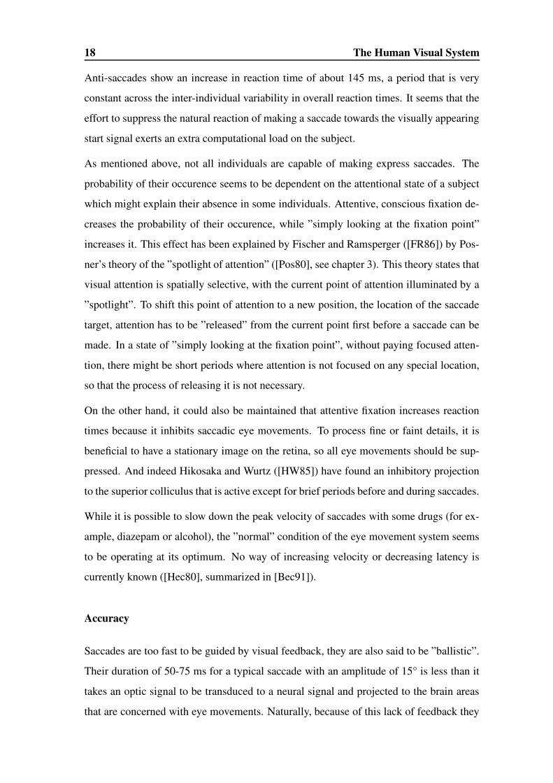
Anti-saccades show an increase in reaction time of about 145 ms, a period that is very
constant across the inter-individual variability in overall reaction times. It seems that the
effort to suppress the natural reaction of making a saccade towards the visually appearing
start signal exerts an extra computational load on the subject.
As mentioned above, not all individuals are capable of making express saccades. The
probability of their occurence seems to be dependent on the attentional state of a subject
which might explain their absence in some individuals. Attentive, conscious fixation de-
creases the probability of their occurence, while ”simply looking at the fixation point”
increases it. This effect has been explained by Fischer and Ramsperger ([FR86]) by Pos-
ner’s theory of the ”spotlight of attention” ([Pos80], see chapter 3). This theory states that
visual attention is spatially selective, with the current point of attention illuminated by a
”spotlight”. To shift this point of attention to a new position, the location of the saccade
target, attention has to be ”released” from the current point first before a saccade can be
made. In a state of ”simply looking at the fixation point”, without paying focused atten-
tion, there might be short periods where attention is not focused on any special location,
so that the process of releasing it is not necessary.
On the other hand, it could also be maintained that attentive fixation increases reaction
times because it inhibits saccadic eye movements. To process fine or faint details, it is
beneficial to have a stationary image on the retina, so all eye movements should be sup-
pressed. And indeed Hikosaka and Wurtz ([HW85]) have found an inhibitory projection
to the superior colliculus that is active except for brief periods before and during saccades.
While it is possible to slow down the peak velocity of saccades with some drugs (for ex-
ample, diazepam or alcohol), the ”normal” condition of the eye movement system seems
to be operating at its optimum. No way of increasing velocity or decreasing latency is
currently known ([Hec80], summarized in [Bec91]).
Accuracy
Saccades are too fast to be guided by visual feedback, they are also said to be ”ballistic”.
Their duration of 50-75 ms for a typical saccade with an amplitude of 15° is less than it
takes an optic signal to be transduced to a neural signal and projected to the brain areas
that are concerned with eye movements. Naturally, because of this lack of feedback they
2.4 Eye Movements 19
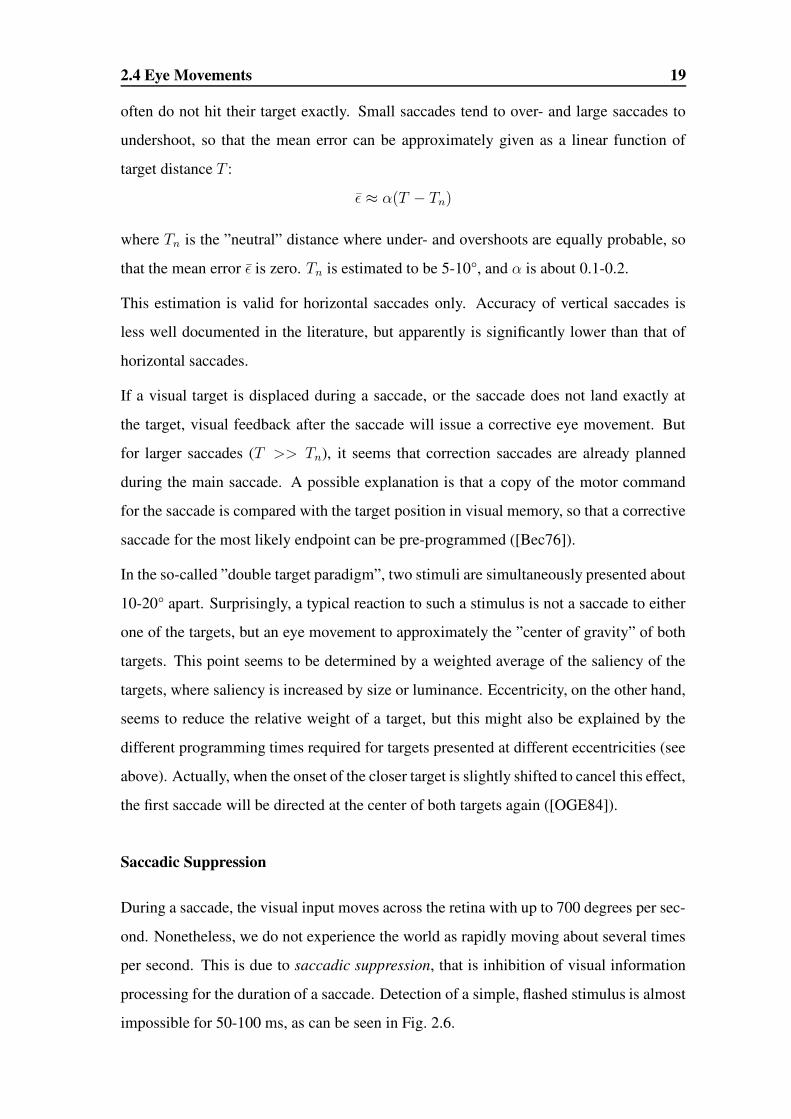
often do not hit their target exactly. Small saccades tend to over- and large saccades to
undershoot, so that the mean error can be approximately given as a linear function of
target distance T :
ε ≈ α(T − Tn)
where Tn is the ”neutral” distance where under- and overshoots are equally probable, so
that the mean error ε is zero. Tn is estimated to be 5-10°, and α is about 0.1-0.2.
This estimation is valid for horizontal saccades only. Accuracy of vertical saccades is
less well documented in the literature, but apparently is significantly lower than that of
horizontal saccades.
If a visual target is displaced during a saccade, or the saccade does not land exactly at
the target, visual feedback after the saccade will issue a corrective eye movement. But
for larger saccades (T >> Tn), it seems that correction saccades are already planned
during the main saccade. A possible explanation is that a copy of the motor command
for the saccade is compared with the target position in visual memory, so that a corrective
saccade for the most likely endpoint can be pre-programmed ([Bec76]).
In the so-called ”double target paradigm”, two stimuli are simultaneously presented about
10-20° apart. Surprisingly, a typical reaction to such a stimulus is not a saccade to either
one of the targets, but an eye movement to approximately the ”center of gravity” of both
targets. This point seems to be determined by a weighted average of the saliency of the
targets, where saliency is increased by size or luminance. Eccentricity, on the other hand,
seems to reduce the relative weight of a target, but this might also be explained by the
different programming times required for targets presented at different eccentricities (see
above). Actually, when the onset of the closer target is slightly shifted to cancel this effect,
the first saccade will be directed at the center of both targets again ([OGE84]).
Saccadic Suppression
During a saccade, the visual input moves across the retina with up to 700 degrees per sec-
ond. Nonetheless, we do not experience the world as rapidly moving about several times
per second. This is due to saccadic suppression, that is inhibition of visual information
processing for the duration of a saccade. Detection of a simple, flashed stimulus is almost
impossible for 50-100 ms, as can be seen in Fig. 2.6.
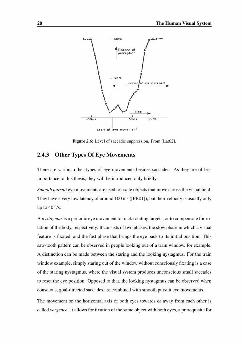
20 The Human Visual System
Figure 2.6: Level of saccadic suppression. From [Lat62].
2.4.3 Other Types Of Eye Movements
There are various other types of eye movements besides saccades. As they are of less
importance to this thesis, they will be introduced only briefly.
Smooth pursuit eye movements are used to fixate objects that move across the visual field.
They have a very low latency of around 100 ms ([PB01]), but their velocity is usually only
up to 40 °/s.
A nystagmus is a periodic eye movement to track rotating targets, or to compensate for ro-
tation of the body, respectively. It consists of two phases, the slow phase in which a visual
feature is fixated, and the fast phase that brings the eye back to its initial position. This
saw-tooth pattern can be observed in people looking out of a train window, for example.
A distinction can be made between the staring and the looking nystagmus. For the train
window example, simply staring out of the window without consciously fixating is a case
of the staring nystagmus, where the visual system produces unconscious small saccades
to reset the eye position. Opposed to that, the looking nystagmus can be observed when
conscious, goal-directed saccades are combined with smooth pursuit eye movements.
The movement on the horizontal axis of both eyes towards or away from each other is
called vergence. It allows for fixation of the same object with both eyes, a prerequisite for

2.4 Eye Movements 21
stereopsis. The velocity of vergent eye movements is fairly slow at around 10 °/s.
Vestibular eye movements are made to maintain fixation of an object while the head or
body moves. Head movements can have peak velocities of up 300 °/s. The head-eye
coordination is controlled by the vestibulo-ocular reflex. This reflex, which is controlled
by information from the vestibular organs, is complemented by the optokinetic reflex,
which is triggered by optical flow.


C H A P T E R 3
Attention
Probably everyone has an intuitive notion about what ”attention” is. This is well-reflected
in everyday phrases such as ”May I have your attention, please?”. Nevertheless, to sci-
entifically define ”attention” is a non-trivial task and there exists a vast body of literature
on the topic. In the following, we will only be able to give a brief overview over some
aspects of research on attention.
One of the first to describe attention from a scientific approach was the psychologist
William James 1890 ([Jam90]), but he only gave an introspective account on his theory of
attention. In his view, attention was mainly concerned with the abstract aspects of sensory
input, such as meaning. Somewhat opposite to this view, von Helmholtz (1866) put an
emphasis on the spatial component of attention ([MT98]).
William James already distinguished two different modes of attention, the ”active” and
the ”passive” mode. In today’s terminology, the active mode correlates to top-down pro-
cesses, where attention towards an object is modulated by an interest in it. The passive
mode correlates to bottom-up processes where attention is purely driven by the sensory
input. James enumerated some stimuli that could evoke attention, for example ”strange
things, moving things, wild animals, [...], blows, blood, etc., etc., etc.” ([Jam90])
A more empirical approach was undertaken by Broadbent ([Bro58], as quoted in [MT98])
who actually wanted to improve communication over noisy channels. He was interested
in what could enhance acoustic perception in the presence of distracting noise. In Broad-
bent’s ”selective filter theory”, certain physical properties of a stimulus, for example the
location or pitch of a sound source, are analyzed in parallel and stored in short term
memory, or, in Broadbent’s words, in the ”S buffer”. Only the behaviourally relevant

24 Attention
information in S is analyzed and transferred to a ”P buffer” where it can be consciously
accessed. The irrelevant information is discarded and cannot be semantically accessed.
That this is a wrong hypothesis has been shown empirically by inserting the subject’s
name into a stream of acoustic material that had to be ignored in an attention study. Sub-
jects did notice this, so that it can be inferred that some semantic analysis happens even
preattentively.
Neisser 1967 ([Nei67], as described in [MT98]) proposed a model of attention that con-
sists of two stages. In the first stage, all sensory input is processed in parallel, while the
second stage serially encodes information into a conscious representation. But Walley
and Weiden ([WW73], as described in [MT98]) have shown that such a second stage does
not need to be serial in nature. A lateral inhibition mechanism, implemented in parallel,
could also prevent irrelevant sources of information from becoming conscious.
Thus, there are two possible principles by which attention could differentiate the process-
ing of attended and unattended objects. Either the attended object receives an enhanced
processing, or the unattended objects are suppressed. With single cell recordings, Moran
and Desimone ([MD85]) found evidence that supported the inhibition theory.
The use of acoustic stimuli to study attention has now declined and most often visual
stimuli are used instead. This is due to the fact that the timing of presentation can be better
controlled with visual stimuli. On the other hand, attention towards acoustic stimuli also
proves a challenging object of study because unlike in vision, there is no way to physically
enhance the resolution of the attended object. In vision, the difference in spatial resolution
across the visual field leads to foveation of an attended stimulus. In hearing, there is no
such equivalent, except for cupping one’s ears.
Today, visual attention is often studied with visual search tasks. Subjects are asked to
search for some specified object, the target, in a display of several objects, the distractors.
This task is a task that also frequently occurs in real world situations and is easily con-
trollable under laboratory conditions. Whenever the subjects have found the target, they
have to press a button. Blank trials where no target is present at all allow to determine the
accuracy of subjects. Of frequent interest is the increase in reaction time with an increase
in the number of distractors. If the reaction time is largely independent of the number
of distractors, the target is said to ”pop out” of the display because it apparently catches

3.1 Spatial Selectivity 25
attention immediately.
This has led to a distinction of ”parallel” and ”serial” processes. The assumption was that
some features could be processed across the whole visual field at once, in parallel, while
others required a serial encoding process. But this dichotomy seems to be outdated now.
A better distinction may be made between ”efficient” and ”inefficient” processes. Many
different studies have found a multitude of different slopes for reaction times, and their
distribution does not seem to be bimodal ([Wol98]).
Two different kinds of cues are used in visual search tasks. Exogenous cues are also called
”pull” cues because they draw attention to their location. Such cues are usually objects
appearing at the location that is to be cued. Endogenous cues, on the other hand, are also
called ”push” cues because subjects have to consciously deploy attention at the location
that is referred to by such a cue. For example, an arrow pointing to the location of interest
or a verbal instruction require an interpreting effort of the subject. Both types of cues
have different effects. Exogenous cues rapidly draw attention, but this effect also decays
very quickly. Endogenous cues, on the other hand, take longer to unfold their effect, but
attention at such a cued location persists for up to several hundred milliseconds ([Yan98]).
As well, there seems to be no ”inhibition of return” for endogenously cued locations.
3.1 Spatial Selectivity
Posner ([Pos80], as described in [Pas98]) has described attention as a spatially selective
process. In this model, attention allows processing of information from a well-defined
spatial region only. If this region is to be changed, triggered by a peripheral signal, at-
tention has to be released from the old location and moved to the new one, ”sweeping”
over the visual field like a spotlight. Thus, shifts of attention are continous. This conse-
quence has been challenged empirically. The duration of shifts of attention seems to be
independent of the amplitude of the shift, so a ”sweep” with constant velocity is unlikely.
As an alternative model that also highlights the spatial component of attention, Eriksen
1986 ([EJ86], as described in [Yan98]) has proposed the ”zoom lens model”. Here, shifts
of attention occur in discrete steps, with an increase of attention at the new location par-
allel to a decrease of attention at the old location. The final size of the attended region

26 Attention
depends on the task at hand.
This hypothesis is supported by a finding by Yantis ([Yan98]), that attention can be spread
over a large region if multiple locations are relevant, with a loss in speed.
3.2 Limits of Attention
As is known from everyday experience, doing several things at once does normally lead
to impaired performance. Consequently, research on attention has shown that attention to
a primary task decreases performance in a second, temporally overlapping task ([MT98]).
We will describe similar phenomena in more detail in chapter 4.
Another limit of attention is that apparently it has a ”refractory period”. Raymond et
al. ([RSA92], as described in [MT98]) presented briefly flashed letters in rapid succes-
sion to subjects. Their task was to detect a white target letter among black letters. After
detection of the target, they should indicate detection of a probe letter, a black ”X”. With-
out the task of detecting the target, this probe letter could easily be detected. But in a
period of 180-270 ms after presentation of the target letter, detection rate for the probe
was very poor. This effect did not occur when the target was followed by a short inter-
val without any visual stimulation at all. The explanation offered by Raymond et al. is
that because of interference of the letters directly following the target with processing of
the target, the attentional system ”blinks” and suppresses that input in order to correctly
process the target letter. Therefore, they called this effect ”attentional blink”.
3.3 Attention and Gaze
Helmholtz already noted that it is possible to deploy attention without fixation. Therefore,
attention and gaze cannot be equated. But it is a reasonable assumption that both under-
lying systems are related, because attended objects normally should be processed with
the highest spatial resolution possible, and it also makes sense that those objects that are
currently available in their highest resolution are attended to. ”We don’t see the location,
but the aspect. On the other hand, we probably won’t see the aspect without the location.”

3.3 Attention and Gaze 27
([ODCR00]) The one exception to this is the possibility to avoid direct eye contact while
covertly monitoring another person that might become dangerous.
In the following, we will briefly present some findings on the relationship of eye move-
ments and attention.
Attention can modulate eye movements. When subjects are presented with two stimulus
patterns simultaneously, a stationary one and a moving one, their eye movements change
depending on the task they are given. If they are to direct attention towards the moving
pattern, their eyes make pursuit movements, while attention towards the stationary pattern
leads to fixations only.
Evidence that a shift in attention to a saccade target prior to the actual eye movement was
found by Currie et al. ([CMCRI95], as quoted in [Hof98]). In a change blindness study
(see chapter 4), changes were made to a scene while the subject was rendered blind during
a saccade because of saccadic suppression. Normally, the detection rate for changes made
under such conditions is poor. But if the saccade endpoint coincided with the location of
the change, subjects were more likely to notice the change. This can only be explained by
a shift in attention before the eye movement. If the change location had been attended to
right before the saccade, and thus the change, it is plausible that the apparent contradiction
in visual input is signalled by the visual system.
Therefore, it can be assumed that attention guides the eyes to those parts of the scene that
are relevant. As well, attention seems to be concerned with the integration of information
from different ’snapshots’ made during fixations.
The saccadic system seems also to be involved even when only covert attention is shifted.
This effect can be derived from studies where shifts of covert attention had to cross ei-
ther the horizontal or vertical meridian of the visual field. For an eye movement across a
meridian, the direction has to be changed because of the anatomy of the oculomotor sys-
tem, while for eye movements inside a hemifield only amplitude is changed. This results
in prolonged reaction times across meridians. And indeed, Rizzolatti et al. ([RRDU87],
as described in [Hof98]) have found such an increase in reaction time, but only for exoge-
nous cues. For endogenous cues, no such increase could be found.

28 Attention
3.4 Capture of Attention
An interesting question especially in the scope of this thesis is what captures attention.
What kind of stimuli can control attention purely from their physical characteristics alone?
As noted above, some types of stimuli seem to ”pop out” from a display, for example
a red target among green distractors. But such an effect can normally only be observed
for very simple stimulus properties, e.g. colour, size, etc. Feature combinations, such as
a red ”L” among green ”L”s and red and green ”T”s, do normally not capture attention,
although capture has been reported for some specific combinations. This has led Yantis
to the formulation that to become a feature singleton, two conditions must be fulfilled: ”a
stimulus that differs from its immediate surround in some dimension, and a surround that
is reasonably homogeneous in that dimension.” ([Yan98]) A difficult problem remains
to estimate what further constraints are put on ”this dimension”, but it seems that task
relevance does play a role.
But the location of such a stimulus is also important. Jonides ([Jon81], as described in
[Yan98]) had subjects perform experiments where cues were either displayed centrally or
peripherally. Because the validity of these cues was very low, i.e. detection of the target
was impaired instead of improved by attending to the cue, subjects should learn to ignore
the cue. In later experiments, subjects were even explicitly told to ignore the cue. While
this was possible for the central cue, the peripheral cues inevitably captured attention, so
that the target detection reaction time increased.
These results and other similar studies suggested the existence of two separate attentional
mechanisms. One is relatively slow, voluntary, and needs a willful effort to be deployed,
the second is involuntary, sets in and decays again rapidly, and responds best to peripheral
stimulation. To study these mechanisms in isolation is difficult because under normal
conditions, ”attention” should be a superposition of these two mechanisms ([Yan98]).

C H A P T E R 4
Blindnesses
From a legal point of view, ”blindness” is defined as a reduction of visual acuity beyond
some threshold. But because of the many different forms visual information processing
has, specific deficits can also give rise to very specific forms of ”blindness”. Some of
these forms are summarized in Table 4.
But what we are interested in are the limits of visual information processing in normal,
healthy subjects. Two examples of such limits can be found in the two bottom entries
in Table 4, ”change blindness” and ”inattentional blindness”. We will now discuss these
phenomena in more detail.
Absolute blindness Absence of any visual information processingLegal blindness An incapacitating reduction of acuityCortical blindness An absence of any conscious visual sensationHemianopia Cortical blindness in one visual hemifieldBlindsight The visual functions that remain in cortical blindnessApperceptive agnosia A disturbance of object visionAssociative agnosia A disturbance of object recognitionProsopagnosia A disturbance of face recognitionChange blindness A disability to detect a change without a temporal transientInattentional blindness An unawareness of a clearly visible object while being
intently engaged in a visual task
Table 4.1: Different forms of ”blindness”. Modified from [Sto96].

30 Blindnesses
4.1 Change Blindness
4.1.1 Phenomena
The study of change blindness dates back to French 1953 ([Fre53]). Although there had
been some ongoing research (e.g. [BHS75]) over the following decades, there was a re-
newed interest in this phenomenon in the nineties. We will now present some of the recent
findings and theories.
Under normal viewing conditions, a retinal transient signals a change. But these retinal
transients can be masked by different means. For example, because of saccadic suppres-
sion, a change made while a subject makes a saccadic eye movement cannot be noticed
by the subject. Blinks render an observer blind for a short period of time (100-200 ms)
as well. Another typical experimental method to cover a retinal transient is the use of
”mudsplashes”. Mudsplashes cover parts of the visual display with large uniform objects,
similar to real mudsplashes on a windshield. Then, there is always the possibility to blank
the entire screen for a short period of time.
Finally, change blindness often occurs even without induction by an experimenter, for
example in movies, where cuts and pans can principally serve the same purpose as the
mudsplashes above. In real-world situations, change blindness can also occur because of
interruptions ([SC99]).
Mainly two different experimental paradigms have been used to investigate change blind-
ness. The ”flicker paradigm” changes back and forth between the altered and the unal-
tered scene until the subject notices the change or a predefined time period has passed.
The time it took the subject or the actual failure to detect the change can then be statis-
tically evaluated. In the ”forced-choice paradigm”, the change is presented only once.
After presentation, the subject is forced to decide whether they detected a change or not.
This paradigm has the advantage that the full psychophysical signal detection theory can
be applied to the data. As a drawback, this paradigm is unable to extract a lot of useful
information about changes that can only be detected after, say, the third presentation on
average.
Both these paradigms allow to study intentional change detection only because the sub-
jects are aware that there will be a change in the course of the experiment. Although

4.1 Change Blindness 31
it is striking that performance is still poor even when subjects are forewarned, of more
interest is the study of incidental encoding, where subjects are not actively searching for
a change. Such experiments can be performed under more natural conditions and are
therefore behaviourally more relevant.
Because of the low peripheral vision of the human visual system as well as because of
memory limits, it is impossible to take in a scene with all its details at once, with one
fixation. Therefore, information about the scene must be encoded to be somehow retained
from one view to the next. This encoding process possibly can only encode a finite number
of aspects or features, but in principle there are infinitely many features in a natural scene.
This makes attention a crucial property for the detection of changes. But mere general
attention is not enough, the attention must be focused towards specific aspects of a scene.
This can be seen from the following experiment where the subjects most likely spent a
large part of their attention on their conversational partner:
A naive subject was approached on the street by one experimenter and asked for direc-
tions. During their conversation, two more experimenters carrying a door passed through,
breaking visual contact. While the first experimenter was hidden from the subject’s view,
he was replaced by one of the door-carriers. Even when the two experimenters differed
significantly in appearance, e.g. height, build, colour of clothes, etc., only 50 % of sub-
jects noted that a change had taken place ([SL97]).
Change detection has been shown to be more likely for changes to objects or aspects that
were in the ”centre of interest” of the presented scene. What constitutes the centre of
interest or only a feature of ”marginal interest” can be determined by asking subjects to
describe the scene. Those aspects that are most often mentioned or that come up first in
the descriptions can also be expected to be encoded early by a subject in the actual change
detection task.
This is consistent with a finding by O’Regan et al. ([ODCR00]) that the probability of
change detection was proportional to the proximity of gaze to the change. At around 6-8°
proximity, change detection performance fell below 10 %. Note, though, that even when
the change took place in the foveal field of vision, performance was only at 60 %.
32 Blindnesses
4.1.2 Possible Explanations
There are five different explanations for change blindness that have been put forward.
None of them fits all experimental data, so it is likely that there exists no single cause for
change blindness, but that there are several processes that can induce change blindness
([Sim00]).
”Overwriting” assumes that the mind engages a memory buffer for visual content. Only
abstract information on a scene gets explicitly represented. The change overwrites parts
of the memory buffer, so that the original content is lost. Only abstractly encoded infor-
mation can be re-encoded from the visual buffer and compared with the previous repre-
sentation.
”First impression” is somewhat the opposite of the overwriting hypothesis. If the task of
the visual system is to extract the abstract meaning of a scene, this goal might have been
achieved already when the change takes place. If this change does not affect the abstract
meaning of the scene, there is no need for this change to be represented in any way. This
hypothesis is supported by experiments where subjects had to describe the scenery they
were presented with during trials. The majority of them described the first, original scene
rather than the altered version of it ([Sim96]).
The ”no comparison” explanation states that both the visual scenery before and after the
change are explicitly represented in the mind, but are not compared if such a comparison
is not explicitly requested. This request might be triggered, under normal circumstances,
by a temporal transient, but also, for example, by an experimenter pointing out an obvious
contradiction. In the ”door experiment” from the section above, this might have been the
question whether the experimenter had not worn a differently coloured hard hat before (of
course, in fact the experimenter and not the hard hat had changed, but the metric of hat
colours allows for more definite statements than the metric of human faces).
Another explanation does away with any internal representation of the visual world at all,
because, according to the ”the world as a memory store” hypothesis, the world itself is
the best possible representation anyway ([ON01]). This hypothesis actually entails a full
philosophical account of many of the epistemological problems that can be found in the
study of vision, but will not be elaborated here any further.
Finally, the ”feature combination” hypothesis is included here for completeness. There

4.2 Inattentional Blindness 33
exists no empirical support for this hypothesis from change blindness experiments, but
other studies still suggest that it might be one of the causes for change blindness. This
hypothesis states that features of the original and the changed scene get merged somehow
in a single integrative buffer, so that the subject has no two different representations at his
hand to compare. Experimental data from eye witness studies, for example, support this
hypothesis.
4.2 Inattentional Blindness
The change blindness paradigm described in the previous section claims that features can
be encoded with attention only. Without attention, not much information is retained across
views.
The theory of inattentional blindness, on the other hand, goes even further and states that
visual perception is impossible at all without attention. ”Observers may fail not just at
change detection, but at perception as well.” ([SC99])
We will briefly present three studies dealing with inattentional blindness here. The first
one to be described here was performed by Mack et al. ([MR98], as described in [SC99])
and gave rise to the inattentional blindness paradigm. They used artificial stimuli, which
allows for precise control of experimental conditions. As a drawback, it is not clear
whether findings can be transferred to real-world behaviour. Therefore, we will also de-
scribe two studies where real world scenes were shown to observers. The inattentional
blindness subjects show in such scenarios is especially striking.
Mack and Rock had subjects perform a relatively simple task, such as judging which of
the two lines of a briefly presented cross is longer. After several trials, another object
appeared at the same time as the cross. About 25% of subjects fail to notice this un-
expected object when the cross is presented at fixation and the unexpected event occurs
parafoveally, although almost all subjects can detect this event in subsequent trials, being
forewarned. The failure rate goes up to 75% when the locations are changed, so that the
cross that is attended to is presented parafoveally and the unexpected object is presented
at fixation. The explanation for this phenomenon by Mack and Rock is that to attend
to the parafoveally presented cross, subjects have to make a willful effort to shift their
34 Blindnesses
attention to this location, which might lead to an increased inhibition of attention at the
fixation point.
Haines ([Hai91], as quoted in [ON01]) examined the effectiveness of head-up displays
in avionics. Commercial aircraft pilots had to land a plane in a flight simulator where
flight information was projected onto the front window, into their normal field of view.
Some pilots could not detect that another plane was present on the runway under these
conditions.
Simons and Chabris ([SC99]) replicated and extended findings made in a study on divided
attention by Neisser et al. ([NB75], as cited in [SC99]). Observers were shown a movie
of two basketball teams passing back and forth two balls. Subjects had to count the
number of passes for the black or white team in the so-called ”easy” task or they had
to simultaneously count the number of aerial passes and bounce passes in the so-called
”hard” task. During the game, unexpected events occur. Such an event could either be
a woman with an umbrella walking across the scene, or a woman in a gorilla costume
entering the scene, thumping her chest directly in front of the camera, and exiting again.
Up to 50% of observers failed to notice such an unexpected event. Not surprisingly, the
detection rate was better for observers who had been assigned the ”easy” task, although
it was still well below 100%. Contrary to what one might expect from ”pop-out” effects
in visual search, where items that visually differ from their surrounding items are easier
to spot, the gorilla with its black body could be detected more easily when the subject’s
task was to watch the black team. Apparently the subjects had focused their attention on
black objects in general, which helped them to detect the gorilla.
4.2.1 Possible Explanations
In the first two experiments described above, inattentional blindness occured because sub-
jects were engaged in a task that apparently consumed all of their attentional resources.
In the ”gorilla” experiment, on the other hand, the visual display consisted of a number
of task-relevant objects (the members of the attended team) as well as a roughly equal
number of distractors. Therefore, subjects had to actively ignore these distracting objects.
This observation leads to two possible explanations of inattentional blindness. The first
is that a clearly visible stimulus is not perceived because it is intentionally ignored, the

4.2 Inattentional Blindness 35
second is that it is not perceived because it differs from the attended object. To experi-
mentally distinguish between these two possibilities is probably a difficult task ([SC99]).
A third, but not very plausible explanation is that subjects consciously perceive the unex-
pected event, but immediately forget it again. While this explanation cannot be disproved
empirically, it can hardly be used to gain more insight into attentional processes.


C H A P T E R 5
Theory
5.1 Preliminaries
An image sequence is defined by its image-intensity function f(x, y, t). For sequences of
colour images, the image-intensity function is
f(x, y, t) =
r(x, y, t)
g(x, y, t)
b(x, y, t)
.
To convert such an image sequence to grayscale images, we can use the image brightness
function
f(x, y, t) =fr + fg + fb
3.
Partial derivatives are denoted fx, fy, ft. Then, the structure tensor ([JHG99]) is
J = ω ∗
f 2x fxfy fxft
fxfy f 2y fyft
fxft fyft f 2t
with ω a spatial smoothing kernel, for example a Gaussian
G(x, y) =1
2πσ2e−
x2+y2
2σ2 .
Image features can be classified according to their intrinsic dimensionality (see Fig. 5.1).

38 Theory
i0D
i1D
i2D
Figure 5.1: Intrinsic dimensionality.
Basically, i0D features are constant in all directions, i1D features exhibit a change in one
direction, and so on.
The informational content of an image sequence can also be classified by its spatio-
temporal curvature.
H = 1/3 ∗ trace(J) = λ1 + λ2 + λ3 = 1/3 ∗ (f 2x + f 2
y + f 2t )
S = M11 +M22 +M33 = λ1λ2 + λ2λ3 + λ1λ3
K = det(J) = λ1λ2λ3
where Mij are the minors of J , obtained by eliminating the 4− i-th row and the 4− j-thcolumn of J , and λk are the eigenvalues of J . H , S, andK allow a simple inference about
the intrinsic dimensionality of a feature. If H 6= 0, the intrinsic dimension is at least 1. It
is at least 2 if S 6= 0, and at least 3 if K 6= 0.
An image sequence is uniquely defined by its intrinsically 2D features ([MB00]). Thus,
it is a useful assumption that these features are also relevant to the observer and therefore
attract gaze ([BKBM04]). Because of S 6= 0 ⇒ H 6= 0, all the information of an image
sequence is (probably redundantly) contained in its curved features where H 6= 0 as well.
This fits with the observation that Yarbus made already, that large areas, usually the fairly
constant ones, of a scene are not fixated at all, but that some features are re-visited by
gaze repetitiously ([Yar67]).
Although we will use the term ”saliency” to denote mean spatio-temporal curvature below,
note that, ultimately, ”saliency” needs to be defined in terms of the attentional relevance.
Because of the top-down influences in perception, this will be hard to achieve in an exact
sense.
5.2 Overview 39
5.2 Overview
Two different image sequence manipulations were implemented. Both were designed
based on theoretical considerations what might attract attention best. Note that in the
following, the term ”stimulus” refers to the image sequence manipulations themselves,
although in a broader sense, the whole image sequence could also be regarded as the
stimulus. Because we want to produce a behavioural change as an effect of the manip-
ulation, while the underlying image sequence remains constant over different trials, we
believe our use of the term stimulus is justified.
The first stimulus type is merely a red dot that replaces a part of the image sequence.
That the colour red is ”popping out” of a display is a well-known fact, see for example its
use in brakelights. The sudden onset of an object also is known to attract attention. The
intensity of the red dot was chosen dependant on the mean brightness of the surrounding
area, so that the local contrast of the stimulus was constant across all locations.
The second stimulus type is derived from the observation that objects approaching a sub-
ject should have a high perceptual relevance. Therefore, this stimulus type magnifies a
part of the scene in a repetitive fashion so that an expanding optical flow is created.
5.3 Stimulus Types
5.3.1 Red Dot Stimulus
For the ”red dot” stimulus, the intensity was determined by the mean brightness of an area
around the stimulus center (xs, ys, ts), multiplied by a contrast factor:
I =c
(2a+ 1)(2b+ 1)
xs+a∑
x=xs−a
ys+b∑
y=ys−bf(x, y, ts)
The stimulus area of the original image sequence was then replaced by
f ′(x, y, t) =
I
0
0

40 Theory
1
1.5
2
2.5
3
0 50 100 150 200
ξ
Time elapsed after stimulus onset in ms
Magnification Factor
Figure 5.2: Function of magnification factor ξ for looming effect.
for x ∈ {xs − a/2, ..., xs + a/2}, y ∈ {ys − b/2, ..., ys + b/2}, where a and b denote, in
pixels, the width and the height, respectively, of the stimulus.
5.3.2 Looming Effect Stimulus
The ”looming effect” stimulus simulates the optical flow of an object approaching the
observer. When an object approaches, its retinal projection expands in size. Here, this
is realized by using the function ippiResizeCenter() of the Intel Performance Primitives
Library, which gives (in a rectangular window around (xs, ys, ts)):
f(x, y, t) = f(xs +x− xsξ(t− ts)
, ys +y − ysξ(t− ts)
, t).
ξ(t) is a saw-tooth function (see Fig. 5.2), so that for the first approximately 130 ms of a
stimulus, the stimulus area gets ”zoomed” closer. Then, the magnification factor drops to
1.0 and the expansion starts again. To account for the fractions of pixel coordinates, cubic
interpolation is used. An example is given in Fig. 5.3.
5.4 Stimulus Placement
For the looming effect to work properly, it was necessary to select a region with at least
some spatial structure. In an almost constant part of the image where fx ' 0 and fy ' 0,
magnification does not change the visual appearance very much, so such regions had to be
excluded from the list of potential stimulus placements. As well, a constant region might
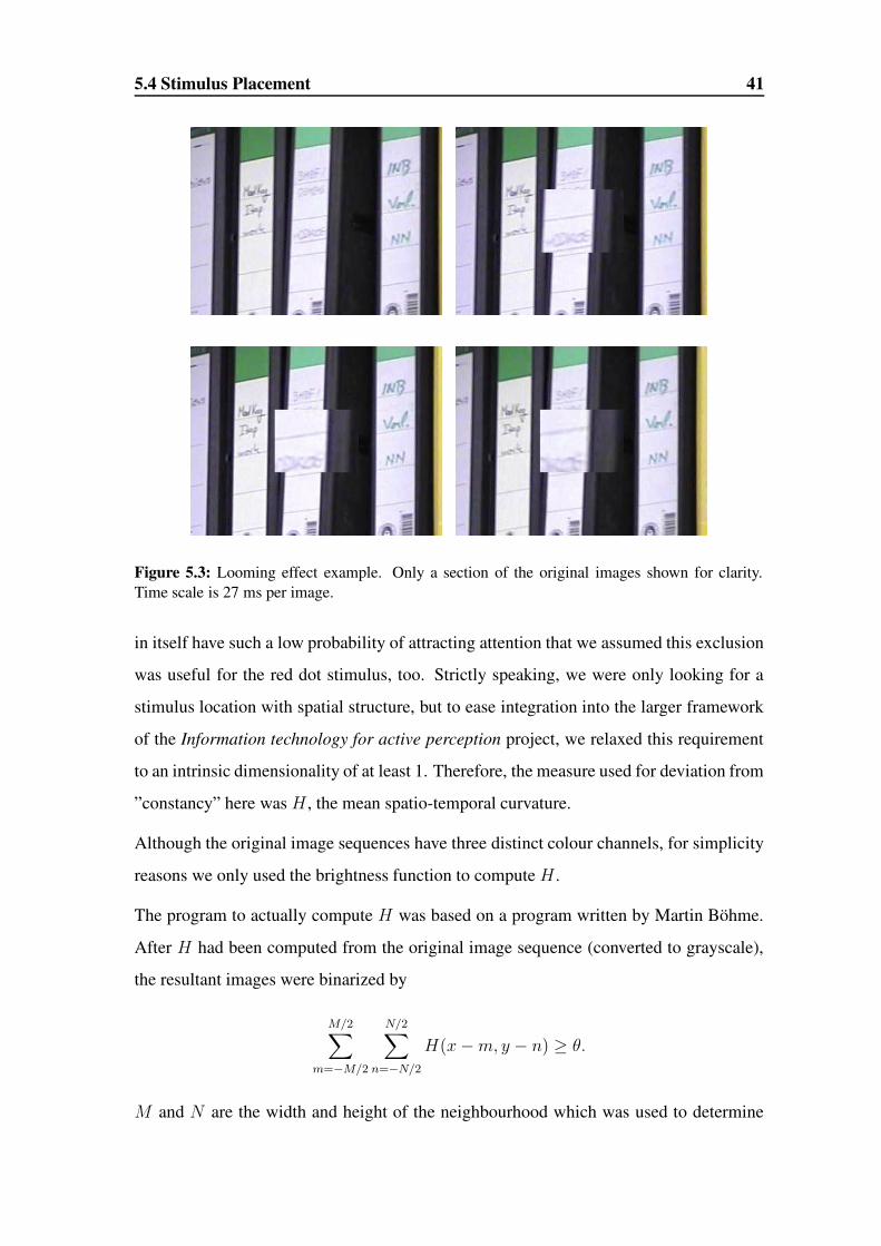
5.4 Stimulus Placement 41
Figure 5.3: Looming effect example. Only a section of the original images shown for clarity.Time scale is 27 ms per image.
in itself have such a low probability of attracting attention that we assumed this exclusion
was useful for the red dot stimulus, too. Strictly speaking, we were only looking for a
stimulus location with spatial structure, but to ease integration into the larger framework
of the Information technology for active perception project, we relaxed this requirement
to an intrinsic dimensionality of at least 1. Therefore, the measure used for deviation from
”constancy” here was H , the mean spatio-temporal curvature.
Although the original image sequences have three distinct colour channels, for simplicity
reasons we only used the brightness function to compute H .
The program to actually compute H was based on a program written by Martin Bohme.
After H had been computed from the original image sequence (converted to grayscale),
the resultant images were binarized by
M/2∑
m=−M/2
N/2∑
n=−N/2H(x−m, y − n) ≥ θ.
M and N are the width and height of the neighbourhood which was used to determine

42 Theory
Figure 5.4: Possible points for stimulus placement around current point of gaze.
Figure 5.5: b) Example for thresholded saliency image. Stimulus placement can be at any whitelocation. a) Original image.
whether there was a minimum amount of saliency around the point (x, y) in question.
The result was down-sampled and stored to disk. In experiments, these saliency images
were then read again by a JPEGBufferProducer (see chapter 6).
For ease of later analysis, the initial distance from the point of gaze at the time of stim-
ulus onset and the stimulus location was always fixed. It was varied only for different
experiments, although the implementation allows for random placement as well. Candi-
date locations for stimuli were therefore randomly drawn from a circle around the current
point of gaze. Because of the strong preference of the human visual system for horizontal
saccades, only locations were considered where the angle between the horizontal axis and
a line between location and point of gaze was less than 45° (see Fig. 5.4).
For these possible locations, a second requirement had to be fulfilled. The locations had
to have a minimum amount of saliency, which was expressed by the saliency image being
white, see Fig. 5.5.
Because it could not be guaranteed that there was always a suitable candidate location, the
algorithm we used simply chose a random location after it had tested 20 possible points

5.5 Stimulus Duration 43
that did turn out to be unsuitable.
5.5 Stimulus Duration
Stimuli were displayed for a maximum of 200 ms. Because their purpose was to attract
the subjects’ gaze while not becoming consciously perceivable, they were switched off
either when the subject made a saccade or the point of gaze came closer to the stimulus
location than 8°. Because saccadic eye movements are made several times per second,
this meant that occasionally the observer started a saccade right after the appearance of
the stimulus, thus switching it off again immediately. These stimuli could not have an
impact and were therefore removed during analysis (see chapter 6).
5.6 Saccade Detection
To be able to detect saccades is a useful feature for several reasons. First, saccadic sup-
pression (see section 2.4.2) renders a subject blind during a saccade, so it does not make
sense to show a short stimulus while the subject is unable to perceive it anyway. More
importantly, after the successful initiation of a saccade towards a stimulus the stimulus
can and should be switched off to reduce the subject’s awareness of it.
Saccades can be detected by a variety of properties such as gaze acceleration or waveform
([TSHB02]), but for the sake of simplicity and low latency the method we used here is
purely velocity-based. Velocity can be computed by
v(t) =√
(xt − xt−1)2 + (yt − yt−1)2
and if two consecutive samples show a velocity above a given threshold
v(t− 1) ≥ θ ∧ v(t) ≥ θ,
it is assumed that a saccade is being made.
From chapter 2, we know that a velocity threshold of around 100°/s would suffice to dis-
criminate saccades from other forms of eye movements. Unfortunately, because of the

44 Theory
high sampling frequency of the eye tracking device, even small inaccuracies in consec-
utive samples give rise to high estimated velocities. This means that with a deviation of
only 0.5° from one sample to the next, the estimated velocity would be 120°/s already.
The eye tracking software allows for a filtering to reduce such noise artefacts, but naturally
this filtering increases latency significantly. Therefore, it was not used in our experiments.
Instead, a fairly high velocity threshold of θ = 160°/s was used.
The latency of the saccade detection therefore is
T = Tet + 2/fet + Trise
with Tet the general latency and fet the sampling frequency of the eye tracker, and Trise
the acceleration time of the eye up to v = θ. With chapter 7 and Trise ≈ 15-20 ms,
we can estimate T to around 33-40 ms. Because of the additional latency of the display,
the overall latency until the system visually responds to a saccade is in the order of 50-
60 ms. For small saccades, this is already in the order of their duration, and because of
the comparatively small size of the visual display unit, these saccades unfortunately tend
to be the most common ones. The exact gain of saccade detection has not been examined,
though.
5.7 Data Analysis
The question how to measure the similarity of two different scan paths has been put for-
ward in the literature, but only few attempts have been made to answer it. There, the
emphasis was put on scan paths for still images. Two main issues arise when comparing
scan paths. First, one needs to define a metric for what makes a single image feature. For
example, when watching the picture of a face, the euclidean distance between the tip of
the nose and an eye is approximately the same as that of the two eyes, but it could be
argued that a saccade from one eye to the nose is highly different than a saccade from one
eye to the other. Second, the time course of fixations has to be taken into account. In how
much differ the scan paths ”left eye - right eye” and ”right eye - left eye”, to stay in our
example?
Thus, modelling of scan paths has normally included a clustering and labelling of image
5.7 Data Analysis 45
features to arrive at a smaller subset of fixation locations. For example, Hacisalihzade et
al. ([HSA92]) have described a Markov model. After clustering of fixation locations, the
probability of transition from one of these clusters to the next can be written in form of a
transition matrix. Such transition matrices can then be computed for different scan paths
and, for example, their absolute difference be taken to measure (dis-)similarity.
Hacisalihzade et al. also gave a different model that made use of string-editing theory.
If every possible fixation location is labelled with a single letter, a sequence of fixations
can be regarded as a string. String-editing theory now allows to compare two strings
by assigning each operation that is needed to transform one string to the other, such as
deletion, insertion, or substitution, a certain penalty. The least sum of penalties is then the
(dis-)similarity of the two strings. It remains an open problem what useful penalties for
the different operations are.
This approach has been extended to dynamic scenes by Blackmon et al. ([BHC+99]).
In this case, the problem of the correct choice of a clustering algorithm is especially
hard because of possible object motion, so that a semantically identical object appears at
different locations.
In our experiments, we have, in some sense, defined a desired scan path that we could
compare to the actual scan path subjects made. But while a normal scan path includes
2-3 eye movements per second, our artifical desired scan path consisted of stimulus loca-
tions that changed only once per second. Because of this and the other methodological
difficulties with scan path comparisons for dynamic scenes, we decided to probe simpler
measures first. In a first attempt to find out whether stimulus presentation had any ef-
fect on eye movements, we cross-correlated the stimulus function s(n) = (sx(n), sy(n))T
with the gaze function g(n) = (gx(n), gy(n))T . Because for finite signals, the energy
term varies with τ , the normalized cross-correlation function
Kx(τ) =
∑Nn=τ(sx(n)gx(n− τ))√∑Nn=τ sx(n)2
∑N−τn=0 gx(n)2
was used with Ky computed analogously. This function measures the similarity of two
signals with different relative shifts τ . Similarity is 1 if both signals are identical, 0 if
they are completely uncorrelated, and -1 if they have the same shape, but different signs.

46 Theory
0 100 200 300 400 500 600 700 800 900 10000
100
200
300
400
500
600
700
Saccade Targets and Stimulus Locations, Projected Along Time
Figure 5.6: Example scatter plot of saccade targets (red crosses) and stimulus locations (bluediamonds), projected along time. Only data for the first few seconds of an experiment shown forclarity.
Because s and g are only positive, we corrected for this by adjusting for the constant
component, so that e.g. s′x(n) = sx(n)− xmax/2.
After this approach had yielded only unsatisfying results, we also tried to interpolate the
stimulus function. In its original version, the cross-correlation compared a fully-defined
signal with one that was defined at only about 20% of time points. Again, this gave no
satisfying results. As we will see in chapter 8, the problem might have been that the
variance of reaction times is high compared to frequency of eye movements. Therefore,
no single shift τ gives rise to a significantly high correlation.
The same problem occured for a comparison of stimulus onsets and saccade onsets.
But that the quantitative measurements we attempted to define did not yield satisfying
results does not mean that there is no qualitative effect. To prove this, we also visualized
raw data in three different ways. The first method is to give a scatter plot of saccade end-
points and stimulus locations, projected along time. This gave us no causal relationship,
but a strong case to suspect an effect (see, for example, Fig. 5.6). The second method is
to plot, for each stimulus, the distance of gaze data from the stimulus location for several
hundred milliseconds after stimulus onset. Examples of this plot are given in chapter 8. A
third possibility is based on the second. The distance distribution can be plotted over time
after stimulus onset in a three-dimensional plot. Examples can also be found in chapter 8.

C H A P T E R 6
System Description
6.1 Functional Specification
The system to be built had to fulfill several requirements. First, gaze had to be measured.
Second, high resolution video clips had to be displayed and manipulated. For these re-
quirements, a minimum of latency was the major design goal. Finally, the software should
be compatible with both the Linux and Microsoft Windows operating systems.
We will first give an overview of the hardware setup used for the system. Because of the
computational complexity of video-based eye-tracking, two workstations were used, one
for tracking of gaze, the other one for display of actual stimuli (see Fig. 6.2). Then, the
software used for the experiments as well as for later data analysis will be presented.
6.2 Hardware
6.2.1 Eye Tracker Workstation
The eye-tracking device used was a commercially available SensoMotoric Instruments
iViewX Highspeed system that comes integrated with a chin-rest to minimize head move-
ments during tracking (see Fig. 6.1). Its temporal resolution is 4.2 ms (240 Hz) with a
future upgrade option to 2.85 ms (350 Hz), and its spatial resolution is approximately
0.5-1°.
The associated workstation was built from off-the-shelf components according to speci-
fications made by SMI, namely an Intel Pentium 4 CPU with hyper-threading running at

48 System Description
Figure 6.1: Picture of the experimental setup. Left: chin-rest with integrated illumination andcamera. Middle: video display unit of the display workstation. Right: screen used to monitortracking.
Eye Video
OperatorVideo Display Unit
Display Workstation Eye Tracker
Gaze Data
Stimuli
Debug Output
Figure 6.2: Schematic of system setup.
2.8 GHz, a Matrox G450 graphics board, 512 MB RAM, and Microsoft Windows 2000
as operating system.
Eye Tracking Algorithm
The iViewX uses the corneal reflex method to track the user’s gaze. That is, an infrared
source is directed at one of the user’s eyes by means of a semi-transparent mirror while at
the same time, an infrared-sensitive CCD camera takes images of the eye. These images
are transferred to the eye-tracking workstation via a EureCard GrabLink framegrabber
card. The infrared beam creates a bright corneal reflex that can be as easily segmented
as the dark pupil (see the cross-hairs in Fig. 6.3). After a calibration (see 6.3.1), gaze
direction can be inferred from the relative position of pupil and corneal reflex.

6.2 Hardware 49
Figure 6.3: Enlarged part of iViewX screenshot. The dark cross-hair centers on the bright spot infront of the pupil, the corneal reflex. The white cross-hair indicates the center of the tracked pupil.The outline of the tracked pupil is given by a white diameter.
For a more detailed overview of eye-tracking methods, see, for example, [DV00].
6.2.2 Display Workstation
The display workstation included an Intel Pentium 4 3.2 GHz CPU with hyper-threading
and 1 GB RAM to allow for real-time image processing, and an Nvidia Quadro FX1000
graphics board that was chosen for its OpenGL support, its capability of high refresh rates,
and its high colour resolution.
As a visual display unit, an Iiyama HM204DT monitor was used because of its high
vertical sync frequency. Other monitors capable of similar refresh rates tend to be much
smaller as the HM204DT has a 22” diagonal that spans a visual field of approximately
44° horizontally and 33° vertically at a viewing distance of 50 cm. Another useful feature
is the possibility to attach two video sources so that the whole setup can be operated by
a single person. First, the eye tracker input can be displayed until the eye tracker is set
up. Then, with the head still fixated, the input can be switched to that of the display
workstation. This proved especially useful during debugging sessions.
The display workstation runs under a standard Linux distribution.
Connection
Eye tracker and display workstations are connected by a dedicated network link. The
display workstation is also integrated into the internet by a second network adapter to
allow for ease of software development and deployment. The network adapters for the
50 System Description
dedicated link are gigabit network interfaces with ”ping” round-trip times of less than
0.1 ms.
The communication is realized by UDP packets containing commands or sample data in
a format defined by SMI ([Ins03]). UDP (User Datagram Protocol) is a connectionless
network protocol with very low overhead such as error correction. It is therefore well-
suited to eye-tracking applications where timely delivery of the majority of packets is
more important than a guaranteed, but slower, delivery for all packets.
6.3 Software
One of the design goals for the software was compatibility with both Windows and Linux
platforms because the current system runs in a network of Linux workstations, but future
versions might become integrated into eye-tracking devices running the Windows oper-
ating system (see above). Therefore, only libraries available on both platforms had to be
chosen.
Generally, the software was written in C++, using the GNU GCC compiler in version
3.3.1. For graphics output, OpenGL was used with the Fast Lightning Toolkit ([FLT]). To
facilitate thread management as well as network protocol support, we used the OpenTop
library ([EOT]). For real-time image processing, the Intel Performance Primitives Library
([IIP]) was used.
6.3.1 Calibration
The iViewX software comes with a built-in calibration facility. Calibration commands
are sent via the UDP link that is also used for the transfer of gaze data. By default, 9
calibration points are used that are displayed sequentially (see Fig. 6.4). After a fixation of
600 ms, the next calibration point is displayed. The order can be randomized. Calibration
points are drawn as red squares with a size of 0.4°×0.4° on a blue background in a FLTK
window.

6.3 Software 51
5%5%
50%
50%
Figure 6.4: Calibration points and their relative positions ([Ins03]).
6.3.2 Coordinate System Transformation
Four different coordinate systems are involved which sometimes made debugging some-
how difficult. There are the coordinate system of the eye tracker (Met × Net), the screen
resolution of the display workstation (Msc × Nsc), the spatial resolution of the image
sequence (Mim × Nim), all with the (0, 0) coordinate in the upper left corner, and the
coordinate system of the OpenGL context that has size (Msc ×Nsc), but with (0, 0) in the
bottom left corner.
Transformation is performed linearly, with rounding to the nearest integer:
xB = round(xAMB/MA), yB = round(xAMB/MA)
6.3.3 Timing
For the high timing resolution needed in this project, a routine was written in assembly
language that facilitates the internal clock cycle counter of x86 processors. This intro-
duces the problem of identical time stamps that represent different points in time for
processors with different clock frequencies, but gives the highest possible precision with
almost no overhead. Two consecutive calls to this routine show that the time spent for one
call takes 36 clock cycles, which is in the order of 10 ns on the hardware described above.
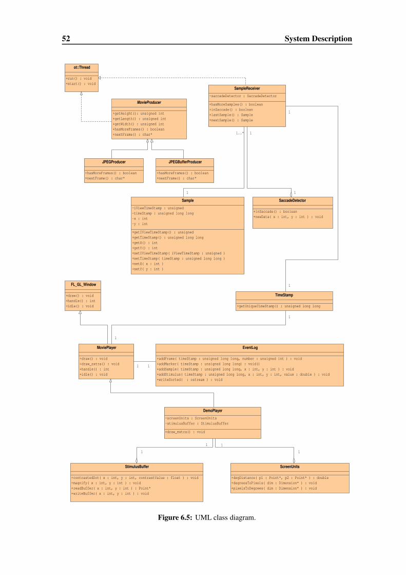
52 System Description
EventLog
+addFrame( timeStamp : unsigned long long, number : unsigned int ) : void+addMarker( timeStamp : unsigned long long) : void()+addSample( timeStamp : unsigned long long, x : int, y : int ) : void+addStimulus( timeStamp : unsigned long long, x : int, y : int, value : double ) : void+writeSorted( : ostream ) : void
StimulusBuffer
+contrastedDot( x : int, y : int, contrastValue : float ) : void+magnify( x : int, y : int ) : void+readBuffer( x : int, y : int ) : Point*+writeBuffer( x : int, y : int ) : void
ScreenUnits
+degDistance( p1 : Point*, p2 : Point* ) : double+degreesToPixels( dim : Dimension* ) : void+pixelsToDegrees( dim : Dimension* ) : void
Sample
-iViewTimeStamp : unsigned-timeStamp : unsigned long long-x : int-y : int
+getIViewTimeStamp() : unsigned+getTimeStamp() : unsigned long long+getX() : int+getY() : int+setIViewTimeStamp( iViewTimeStamp : unsigned )+setTimeStamp( timeStamp : unsigned long long )+setX( x : int )+setY( y : int )
DemoPlayer
-screenUnits : ScreenUnits-stimulusBuffer : StimulusBuffer
+draw_extra() : void
TimeStamp
+getUniqueTimeStamp() : unsigned long long
SaccadeDetector
+inSaccade() : boolean+newData( x : int, y : int ) : void
SampleReceiver
-saccadeDetector : SaccadeDetector
+hasMoreSamples() : boolean+inSaccade() : boolean+lastSample() : Sample+nextSample() : Sample
MovieProducer
+getHeight(): unsigned int+getLength() : unsigned int+getWidth() : unsigned int+hasMoreFrames() : boolean+nextFrame() : char*
JPEGProducer
+hasMoreFrames() : boolean+nextFrame() : char*
JPEGBufferProducer
+hasMoreFrames() : boolean+nextFrame() : char*
MoviePlayer
+draw() : void+draw_extra() : void+handle() : int+idle() : void
FL_GL_Window
+draw() : void+handle() : int+idle() : void
ot::Thread
+run() : void+start() : void
1
1
1
1
1
1
1
1
1
1..*
1
1
11
Figure 6.5: UML class diagram.
6.3 Software 53
6.3.4 Classes
The class diagram for the system can be found in Fig. 6.5. Only the important classes and
methods are shown, the less important ones are omitted for clarity. We will also give a
short description of these classes in the following.
The class that is responsible for actually drawing images to the screen is MoviePlayer.
Pointers to the images are received from a MovieProducer instance. When such a frame
needs to be drawn is determined by the number of vertical refreshes elapsed in combina-
tion with the current time stamp (see above). This class also takes care of user interaction
issues such as control of keyboard input.
For each vertical refresh event, this class calls a method draw extra() that can be overri-
den by derived classes to actually implement gaze-contingent behaviour.
One such class is DemoPlayer. In Fig. 6.5, two more classes are depicted that Demo-
Player is composed of. One is StimulusBuffer, which is responsible for image manip-
ulations at given locations with methods contrastedDot() and magnify(). A thorough
description of what these methods do can be found in chapter 5. The other member class
is ScreenUnits. This class defines useful methods for converting between screen units
such as pixels, and real-world units such as degrees of visual angle.
MovieProducer is the base class that defines methods to generate a sequence of images
that can be handed over to a MoviePlayer. In the present system, this generation is limited
to reading a sequence from hard disk, but derived classes could create synthetic sequences
”on-the-fly” as well.
The class JPEGProducer inherits from MovieProducer. It reads and decodes into mem-
ory a set of consecutively numbered JPEG images. To balance the workload during thread
execution, JPEGProducer contains an internal queue of already decoded images. If the
length of this queue reaches a pre-defined limit, this thread blocks until images are con-
sumed.
Because the use of a standard JPEG decoder implementation ([Gro]) turned out to be a
bottleneck, it was replaced by a modified version of the Intel IPP sample JPEG decoder
([IIP]). This decreased image loading times for high definition videos from approximately
45 ms to 16 ms.

54 System Description
JPEGBufferProducer gives an extra increase in speed. Decompressed JEPG images
are buffered in memory. For higher resolution or longer image sequences, this poses a
problem, though. One second of uncompressed HDTV video (30 Hz, 1200×720 spatial
resolution, 3 colour channels) takes up ca. 74 MB of memory. This makes it unsuitable
to buffer any movies longer than about 10 seconds. On the other hand, the saliency
information for the movies is also stored in JPEG image sequences, but with a much lower
resolution (300×160 spatial resolution, one colour channel only). Here, one second takes
up about 1.4 MB of memory, so that it becomes feasible to buffer the whole saliency
information. This is especially useful as it decreases the number of hard disk accesses by
50%.
The EventLog is responsible for data collection during an experiment. The events that
make up the data are described in 6.3.5. In the current implementation, this class only
holds a number of variable-sized vectors for each event type. After an experiment, these
events are sorted in chronological order and written to disk. For very long experiments, it
might be useful to implement a strategy that writes the data to disk in given intervals, to
reduce memory usage at a minimum cost of hard disk accesses.
Class SampleReceiver implements a thread that waits on a network socket for the in-
coming gaze data. Gaze data is modelled by class Sample. They are sent by the eye
tracker workstation with spatial coordinates and a time stamp from the iViewX software.
In SampleReceiver, samples are attached another time stamp to document the exact
point in time of their availability on the display workstation and stored in a ring buffer.
Emptiness of this ring buffer can be checked with the hasMoreSamples() method.
Should the buffer become full (a situation that should not arise anyway for reasonable
buffer sizes), this thread does not block, but old entries in the buffer are overwritten. This
is to ensure that the most recent data are always available. Access to the buffer is regulated
by mutexes. This class also incorporates saccade detection by means of a SaccadeDe-
tector class. Saccade detection was discussed in detail in section 5.6.
6.3.5 Data Analysis
After an experiment, the resultant data is stored as a chronological list of events in an
ASCII file. The processing of these data was implemented in a package of Java classes

6.3 Software 55
for ease of implementation.
De-Noising of Eye Movement Data
The main source of noise in eye movement data is due to blinks. With the eyelid closed,
the eye tracker cannot locate the pupil anymore and sends samples with coordinates (0,0)
to the display workstation. During the analysis phase, these samples are removed from
a SampleContainer by the class BlinkFilter. If, by accident, some valid samples with
zero-coordinates should have been removed, this should not pose too much of a problem
because the samples right before and after the ones in question will show coordinates
close to zero. The subsequent interpolation of sample data (see below) will then fill the
resultant gap with an approximation to the correct values.
Another source of noise is the temporary loss of the correct tracking of pupil or corneal
reflex, for example when some random bright spot in the eye is mistaken for the corneal
reflex. This often leads to gaze coordinates that are outside the calibrated area of the
visual display unit. Thus, samples where sx /∈ [0,Met) ∨ sy /∈ [0, Net) are discarded.
A problem that remains is loss of accuracy of the eye tracker that results in coordinates
inside the valid rectangle. This can only be avoided by the experimenter closely monitor-
ing the tracking process during an experiment. The iViewX software outlines the detected
and tracked pupil and corneal reflex in real time (see Fig. 6.3). Sometimes completely dif-
ferent image features are mistakenly tracked instead of pupil or corneal reflex, or slightly
wrong thresholds have been selected so that the size and shape of the detected features
vary greatly with small changes in illumination or eye position. If the tracking seems
to be insufficient, parameters such as camera gain or segmentation thresholds have to be
adapted to improve tracking quality.
As a final step in pre-processing the data, the class SampleInterpolator can be used to
interpolate the filtered data. First, gaps in the data are filled in with a linear interpolation
of the samples before and after the gap. Then, all samples are filtered with a Gaussian
kernel of variable length.

56 System Description
Event Types and Storage
The different types of events that can happen during an experiment share some character-
istics regardless of their specific type. Therefore, they were modeled in a class hierarchy
with Event as a base class. Such an event mainly possesses a time stamp, which is orig-
inally stored in cpu clock cycles resolution. When reading in from the data file, it is
converted to milliseconds resolution. Furthermore, an event has a method compareTo()
that allows to determine the chronological order of two different events. This is espe-
cially useful for events such as stimuli. Because a stimulus event is generated for each
frame the stimulus is visible in, one stimulus consists of many single event entries with
different time stamps in the data file. For the analysis, these entries are merged to one
StimulusEvent with an onset and an offset time stamp.
The different event types that inherit from Event will be described below. To store the
events in memory, they are inserted into a sorted binary tree structure. This data structure
is implemented in class EventContainer. An array of fixed size might be a more intuitive
data structure for events, but the use of a tree allows for easier insertion and removal of
events, which proves especially useful for filters. As well, some event types are extremely
sparse, for example marker events that occur every 20 s only. To store these in an array
with milliseconds resolution would be significantly inefficient. With a sorted tree, it is also
possible to cut out ”windows”, e.g. the second following some event, very efficiently.
SampleEvent and StimulusEvent both inherit from PointEvent which, in turn, inherits
from Event. A PointEvent has two-dimensional spatial coordinates. The same interpo-
lation and filtering routines can therefore be applied to samples and stimuli. StimulusEv-
ents also have, as noted above, a duration rather than a single time stamp. Thus, onset
and offset are stored explicitly.
The class FrameEvent mainly serves timing purposes. A FrameEvent is emitted at
every buffer swap of the visual display unit, so that, for example, a single StimulusEvent
is visible at least from the time stamp of the following FrameEvent to the time stamp
of the one after that. By computing the time difference between two FrameEvents, it is
also possible to detect periods where the system slowed down so much that it dropped
frames, for example due to background (system) processes. Additionally, this class stores
an index to the specific image that was shown at the associated time.

6.3 Software 57
MarkerEvents can be used to mark specific time points in a data set, for example the
repetition of a presented image sequence.
EventFilter is a base class for non-linear filters that remove invalid events. Derived
classes are BlinkFilter which removes blinks, ShortStimulusFilter that allows to dis-
card extremely short stimuli if stimulus onset and a saccade coincided accidentally, and
StimulusTypeFilter which is used to separate different types of stimuli.
Linear filters like EventInterpolator implement the base class EventProcessor.
The class EventContainer was described above already. It is responsible for efficient
storage of events.
A SaccadeEvent is similar to a stimulus event in that it has an onset and an offset. De-
tection of saccades during analysis was similar to saccade detection during an experiment
(see 5.6), except that different thresholds for onset and offset of a saccade were used.

C H A P T E R 7
Timing Validation
To be able to immediately react to eye movements is obviously a crucial feature of a gaze-
contingent system. As of now, it is still unknown what the exact upper bound of latency
is for such a system as proposed in this thesis. A first approximation can probably given
by the fact that, as we have seen in section 2.4.2, saccadic suppression renders a person
blind for about 50-100 ms. Therefore, it is desirable to have an end-to-end latency from
the onset of the eye movement to the stimulus drawn on the screen of less than 50 ms.
To estimate the latency of our system, we will first model the basic processing chain of our
system in this chapter. Then, we will give some measured data to validate this estimation.
7.1 Theory
The end-to-end latency of the whole system can be estimated as
Toverall = Ttracker + Ttransfer + Tdisplay.
The latency of the SMI iViewX Highspeed eye tracker is specified with 8 ms for the
system running at f = 350 Hz and with 10 ms for the system used in our experiments,
running at f = 240 Hz ([Leh03]). These numbers are composed as follows:
Ttracker = Tccd + Tgrab + Tproc + Tmap
Tccd is the exposure time of the camera and depends on the frequency of the system:
Tccd = 1/f = 4.166 ms. Tgrab is the time required to grab the analogue camera output
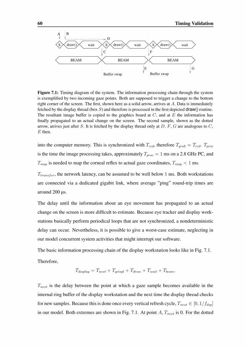
60 Timing Validation
S wait S wait Sdraw() draw() draw() wait
C F
E G
BEAM BEAM BEAM
Buffer swap Buffer swap
A BD
Figure 7.1: Timing diagram of the system. The information processing chain through the systemis exemplified by two incoming gaze points. Both are supposed to trigger a change to the bottomright corner of the screen. The first, shown here as a solid arrow, arrives at A. Data is immediatelyfetched by the display thread (box S) and therefore is processed in the first depicted draw() routine.The resultant image buffer is copied to the graphics board at C , and at E the information hasfinally propagated to an actual change on the screen. The second sample, shown as the dottedarrow, arrives just after S. It is fetched by the display thread only at D. F , G are analogous to C ,E then.
into the computer memory. This is synchronized with Tccd, therefore Tgrab = Tccd. Tproc
is the time the image processing takes, approximately Tproc = 1 ms on a 2.8 GHz PC, and
Tmap is needed to map the corneal reflex to actual gaze coordinates, Tmap < 1 ms.
Ttransfer, the network latency, can be assumed to be well below 1 ms. Both workstations
are connected via a dedicated gigabit link, where average ”ping” round-trip times are
around 200 µs.
The delay until the information about an eye movement has propagated to an actual
change on the screen is more difficult to estimate. Because eye tracker and display work-
stations basically perform periodical loops that are not synchronized, a nondeterministic
delay can occur. Nevertheless, it is possible to give a worst-case estimate, neglecting in
our model concurrent system activities that might interrupt our software.
The basic information processing chain of the display workstation looks like in Fig. 7.1.
Therefore,
Tdisplay = Tnext + Tgetspl + Tdraw + Twait + Tbeam.
Tnext is the delay between the point at which a gaze sample becomes available in the
internal ring buffer of the display workstation and the next time the display thread checks
for new samples. Because this is done once every vertical refresh cycle, Tnext ∈ [0, 1/fdsp]
in our model. Both extremes are shown in Fig. 7.1. At point A, Tnext is 0. For the dotted

7.2 Measurements 61
arrow, it is D − B, almost 1/fdsp. Unfortunately, because of other processes running
in the background, Tnext can also be unpredictably higher. To estimate this effect, real
measurements will be presented below.
Tgetspl is in the order of a few microseconds and is included here only to denote the
important points in time A and D.
Stimuli have to be drawn and video frames have to be copied from memory to the graphics
board. For full video frames, which have only to be updated at 30 Hz, this gives Tdraw =1-
2 ms, and much less than 1 ms for mere stimulus drawing. These estimations are based
on comparing time stamps at entry to and exit of the actual drawing routines.
The display uses double buffering to avoid tearing effects. Therefore, for every vertical
refresh, fore- and background buffers are swapped. Twait is the time until the next buffer
swap occurs, Twait ∈ [0, 1/fdsp].
The image is finally drawn to the screen by an electron beam that traverses the frontal
glass pane of the screen from the top left to the bottom right corner. The contents of the
bottom right corner are therefore updated only at the very end of a vertical screen refresh
cycle. Thus, Tbeam ∈ [0, 1/fdsp].
Therefore, we can estimate Tdisplay to somewhere between 2/fdsp and 3/fdsp, depending
on the location we want to change. At fdsp = 150 Hz, this equals to 13 to 20 ms.
With these numbers, we can now estimate Toverall to 30 ms.
7.2 Measurements
To validate these theoretical considerations, we did some practical measurements. The
procedure we used loosely follows the one described in [TSHB02].
The iViewX eye tracker comes equipped with a DAQCard PIO/DIO48 digital input/output
card and the ability to trigger a TTL output whenever the gaze coordinates are inside an
arbitrarily definable polygon, the area of interest. Taking into account the eye tracker
latency of roughly 10 ms (see above), we therefore had a reliable means of detecting
a specific point in time, namely the crossing of the area of interest borders of an eye
movement.
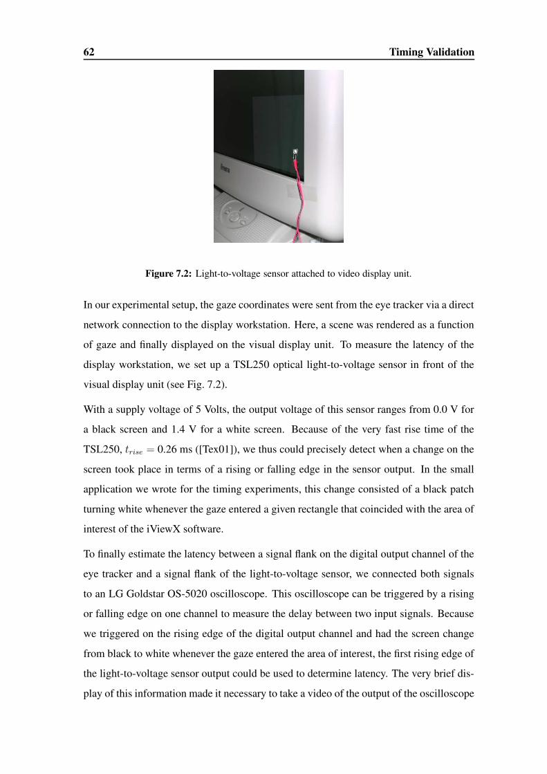
62 Timing Validation
Figure 7.2: Light-to-voltage sensor attached to video display unit.
In our experimental setup, the gaze coordinates were sent from the eye tracker via a direct
network connection to the display workstation. Here, a scene was rendered as a function
of gaze and finally displayed on the visual display unit. To measure the latency of the
display workstation, we set up a TSL250 optical light-to-voltage sensor in front of the
visual display unit (see Fig. 7.2).
With a supply voltage of 5 Volts, the output voltage of this sensor ranges from 0.0 V for
a black screen and 1.4 V for a white screen. Because of the very fast rise time of the
TSL250, trise = 0.26 ms ([Tex01]), we thus could precisely detect when a change on the
screen took place in terms of a rising or falling edge in the sensor output. In the small
application we wrote for the timing experiments, this change consisted of a black patch
turning white whenever the gaze entered a given rectangle that coincided with the area of
interest of the iViewX software.
To finally estimate the latency between a signal flank on the digital output channel of the
eye tracker and a signal flank of the light-to-voltage sensor, we connected both signals
to an LG Goldstar OS-5020 oscilloscope. This oscilloscope can be triggered by a rising
or falling edge on one channel to measure the delay between two input signals. Because
we triggered on the rising edge of the digital output channel and had the screen change
from black to white whenever the gaze entered the area of interest, the first rising edge of
the light-to-voltage sensor output could be used to determine latency. The very brief dis-
play of this information made it necessary to take a video of the output of the oscilloscope

7.2 Measurements 63
Figure 7.3: Example still shot from video. Estimated end-to-end latency here is 27 ms. The wholewidth of the display equals 50 ms, the first rising edge thus occurs at 17 ms, add 10 ms latency ofthe eye tracker.
while a subject made constant eye movements in and out of the area of interest. This video
was then examined later on frame by frame (for an example, see Fig. 7.3). To reduce the
number of frames that had to be examined, we used the fact that all the relevant infor-
mation was in the green trace of the oscilloscope. Therefore, we wrote a little program
that sorted out all those frames where the maximum value of the green colour channel did
not exceed some threshold. This reduced the number of frames to be examined by about
98%.
For results with fdsp = 85 Hz, see Fig. 7.4(a).
These results are in accordance with the theoretical considerations made above.
Nevertheless, because of the low complexity of the scene to be rendered, these results
might not be representative for real experiments. To increase the load of the system, we
performed two steps. First, we increased the screen refresh rate from 85 Hz to 150 Hz.
Now, the duration of a single refresh cycle was reduced from 11.7 ms to 6.6 ms, so that
even small system interrupts of a few milliseconds might lead to an extra refresh cycle of
latency. Second, to mimick the system load of real experiments, we had the system load
and display high resolution movies. The black or white patch was simply drawn on top of
the image sequence.
The results for these extra conditions are shown in Fig. 7.4(b) and Fig. 7.4(c). Again,
these data clearly fit the model that predicted latencies between 2/fdsp and 3/fdsp. In
Fig. 7.4(c), the distribution is slightly shifted to the right because of extra system load.
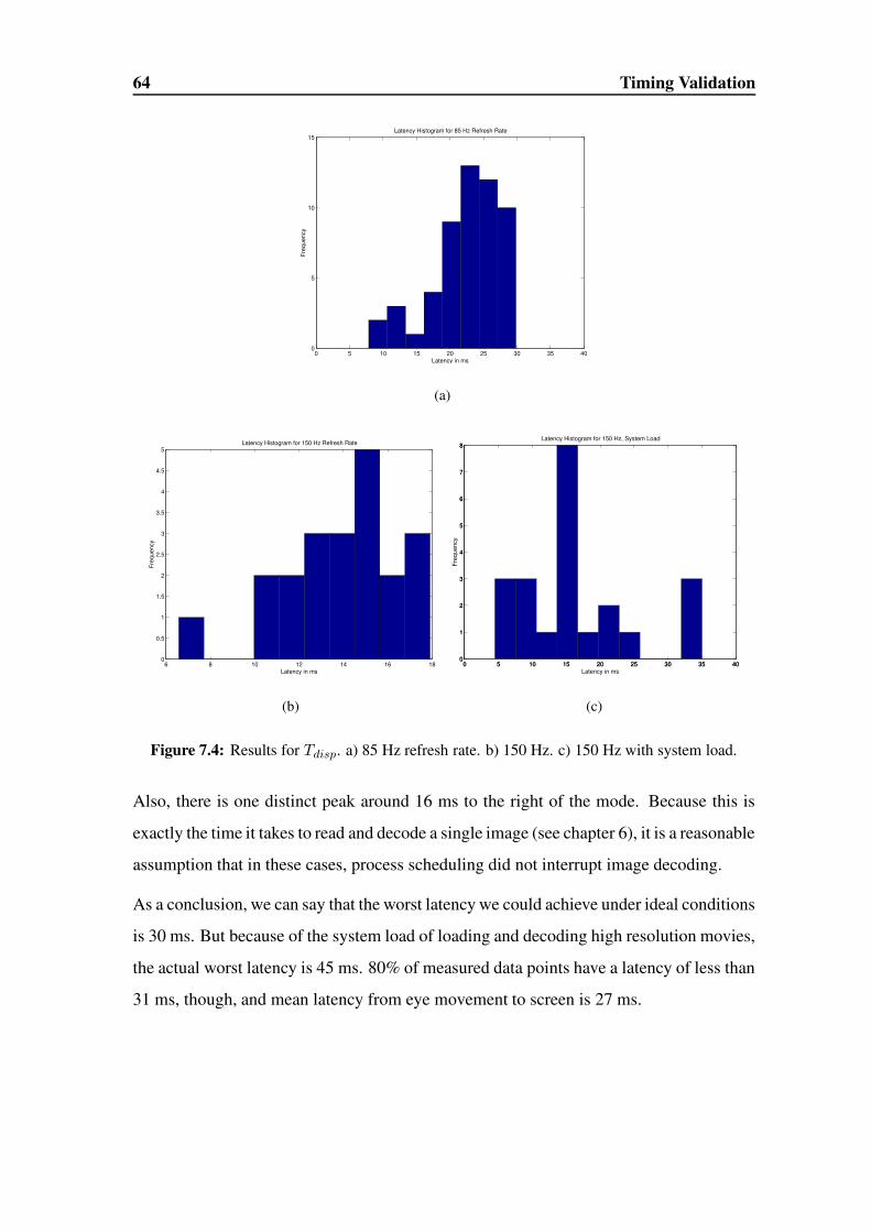
64 Timing Validation
0 5 10 15 20 25 30 35 400
5
10
15
Latency in ms
Freq
uenc
y
Latency Histogram for 85 Hz Refresh Rate
(a)
6 8 10 12 14 16 180
0.5
1
1.5
2
2.5
3
3.5
4
4.5
5Latency Histogram for 150 Hz Refresh Rate
Latency in ms
Freq
uenc
y
(b)
0 5 10 15 20 25 30 35 400
1
2
3
4
5
6
7
8Latency Histogram for 150 Hz, System Load
0 5 10 15 20 25 30 35 400
1
2
3
4
5
6
7
8
Latency in ms
Freq
uenc
y
(c)
Figure 7.4: Results for Tdisp. a) 85 Hz refresh rate. b) 150 Hz. c) 150 Hz with system load.
Also, there is one distinct peak around 16 ms to the right of the mode. Because this is
exactly the time it takes to read and decode a single image (see chapter 6), it is a reasonable
assumption that in these cases, process scheduling did not interrupt image decoding.
As a conclusion, we can say that the worst latency we could achieve under ideal conditions
is 30 ms. But because of the system load of loading and decoding high resolution movies,
the actual worst latency is 45 ms. 80% of measured data points have a latency of less than
31 ms, though, and mean latency from eye movement to screen is 27 ms.
C H A P T E R 8
Results
8.1 Movies
The system was tested with several movie clips. Exemplary, we will present three of them
here.
The first movie (see Fig. 8.1) shows a slow camera pan across a bookshelf and parts of
a desktop. No objects move, so the intrinsic saliency is low. This movie has a temporal
resolution of 30 Hz and is 600 frames long. Its spatial resolution is 320×240 pixels and
therefore this movie shows relatively little detail.
The second movie, illustrated in Fig. 8.2, shows a camera pan across a long queue of
people waiting for entrance to the Hospital of the Holy Spirit in Lubeck. People and cars
pass by, so this scene contains a high amount of saliency in the sense of spatio-temporal
curvature. But there is also a lot of ”meaning” extractable from this scene. For example,
the faces of the people are natural attractors for the subjects’ gaze. This movie also has
a spatial resolution of 320×240 pixels, a temporal resolution of 30 Hz, and a duration of
20 s.
The third movie was shot in the HDTV format at 1200×720 pixels. It shows two cars
passing each other on a parking lot, so there is some motion in this scene. The temporal
resolution is 30 Hz again, but the duration of the movie is only 10 s.
All movies were presented at a size of 44°×33°, five times in a row. The first four pre-
sentations were changed by the stimuli described above, the last presentation contained
no stimuli and was used to allow for measurement of ”normal” eye movements for this
scene.
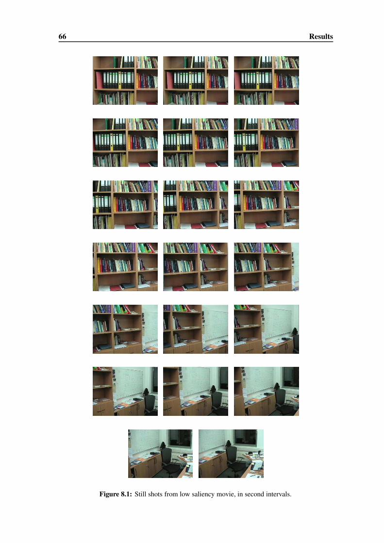
66 Results
Figure 8.1: Still shots from low saliency movie, in second intervals.
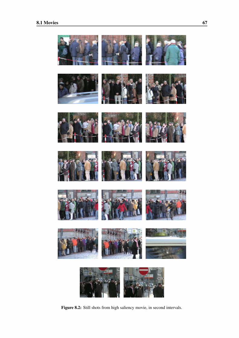
8.1 Movies 67
Figure 8.2: Still shots from high saliency movie, in second intervals.
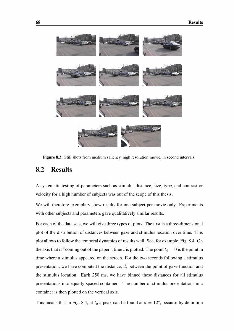
68 Results
Figure 8.3: Still shots from medium saliency, high resolution movie, in second intervals.
8.2 Results
A systematic testing of parameters such as stimulus distance, size, type, and contrast or
velocity for a high number of subjects was out of the scope of this thesis.
We will therefore exemplary show results for one subject per movie only. Experiments
with other subjects and parameters gave qualitatively similar results.
For each of the data sets, we will give three types of plots. The first is a three-dimensional
plot of the distribution of distances between gaze and stimulus location over time. This
plot allows to follow the temporal dynamics of results well. See, for example, Fig. 8.4. On
the axis that is ”coming out of the paper”, time t is plotted. The point t0 = 0 is the point in
time where a stimulus appeared on the screen. For the two seconds following a stimulus
presentation, we have computed the distance, d, between the point of gaze function and
the stimulus location. Each 250 ms, we have binned these distances for all stimulus
presentations into equally-spaced containers. The number of stimulus presentations in a
container is then plotted on the vertical axis.
This means that in Fig. 8.4, at t0 a peak can be found at d = 12°, because by definition
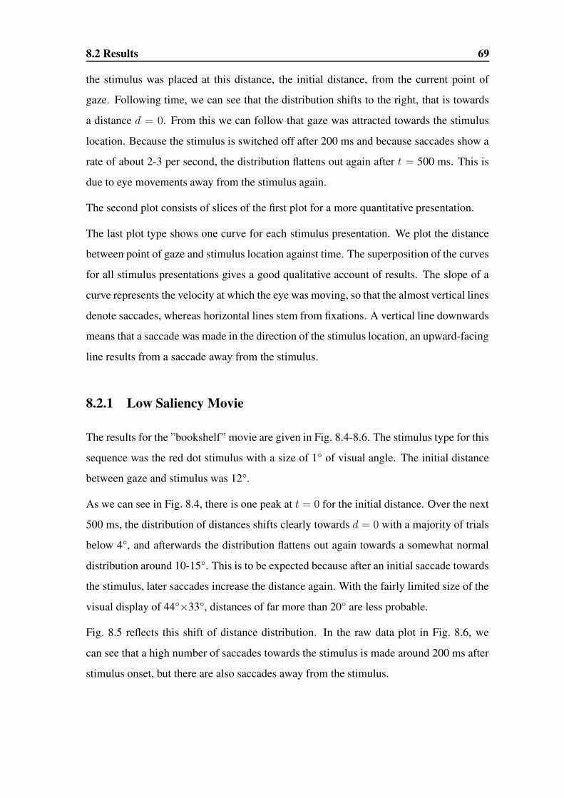
8.2 Results 69
the stimulus was placed at this distance, the initial distance, from the current point of
gaze. Following time, we can see that the distribution shifts to the right, that is towards
a distance d = 0. From this we can follow that gaze was attracted towards the stimulus
location. Because the stimulus is switched off after 200 ms and because saccades show a
rate of about 2-3 per second, the distribution flattens out again after t = 500 ms. This is
due to eye movements away from the stimulus again.
The second plot consists of slices of the first plot for a more quantitative presentation.
The last plot type shows one curve for each stimulus presentation. We plot the distance
between point of gaze and stimulus location against time. The superposition of the curves
for all stimulus presentations gives a good qualitative account of results. The slope of a
curve represents the velocity at which the eye was moving, so that the almost vertical lines
denote saccades, whereas horizontal lines stem from fixations. A vertical line downwards
means that a saccade was made in the direction of the stimulus location, an upward-facing
line results from a saccade away from the stimulus.
8.2.1 Low Saliency Movie
The results for the ”bookshelf” movie are given in Fig. 8.4-8.6. The stimulus type for this
sequence was the red dot stimulus with a size of 1° of visual angle. The initial distance
between gaze and stimulus was 12°.
As we can see in Fig. 8.4, there is one peak at t = 0 for the initial distance. Over the next
500 ms, the distribution of distances shifts clearly towards d = 0 with a majority of trials
below 4°, and afterwards the distribution flattens out again towards a somewhat normal
distribution around 10-15°. This is to be expected because after an initial saccade towards
the stimulus, later saccades increase the distance again. With the fairly limited size of the
visual display of 44°×33°, distances of far more than 20° are less probable.
Fig. 8.5 reflects this shift of distance distribution. In the raw data plot in Fig. 8.6, we
can see that a high number of saccades towards the stimulus is made around 200 ms after
stimulus onset, but there are also saccades away from the stimulus.

70 Results
8.2.2 High Saliency Movie
The results for the ”queue” movie are given in Fig. 8.7-8.9. The initial distance between
gaze and stimulus was 20°, and the looming stimulus that was used for this sequence had
a size of 2°.
Results are less clear than in the low saliency movie, but nevertheless there are some
saccades directed to the stimulus. It is reasonable to assume that saccades that led to a
distance of 4° and less were actually directed at the stimulus. Because of stimulus size, it
is unlikely that saccades will go directly to the center of the stimulus, and the mean error
of a 20° saccade is about 2° alone (see chapter 2). With this assumption, we can say that
about 25% of stimuli provoked an eye movement towards them. Reaction times of these
saccades are higher than in the low saliency movie, as can be seen from the fact that in
Fig. 8.8(b), after 250 ms there is hardly any effect visible, whereas in Fig. 8.8(c), after
500 ms there is a distinct peak close to d = 0. This increased latency might at least in
part be explained by the generally increased reaction time for eccentric presentation (see
chapter 2).
A discernible characteristic in Fig. 8.9 is the high number of lines with a slightly tilted
slope that spread out from the onset. Because this movie shows a camera pan across
a scene, these lines show smooth pursuit movements where objects in the scene were
tracked.
8.2.3 Invisible Stimuli As Baseline Reference
Especially for the high saliency movie, one could argue that the saccades towards the
stimulus locations are a random effect only. By choosing only points with some mean
spatio-temporal curvature as stimulus locations, we have already given a preference to
those points that are more likely to be saccade endpoints anyway. To give a baseline
reference what the results should look like if stimulation had no effect at all, we used
another stimulus type, the ”invisible” stimulus. This stimulus type simply means that the
image sequence was not changed at all, but that stimulus placement and data collection
were performed as in the other experiments.
The parameters for this experiment were the same as for the ”high saliency” experiment in
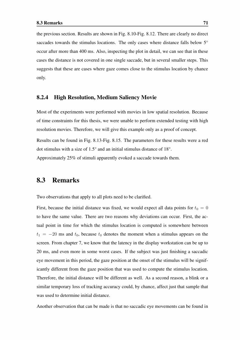
8.3 Remarks 71
the previous section. Results are shown in Fig. 8.10-Fig. 8.12. There are clearly no direct
saccades towards the stimulus locations. The only cases where distance falls below 5°
occur after more than 400 ms. Also, inspecting the plot in detail, we can see that in these
cases the distance is not covered in one single saccade, but in several smaller steps. This
suggests that these are cases where gaze comes close to the stimulus location by chance
only.
8.2.4 High Resolution, Medium Saliency Movie
Most of the experiments were performed with movies in low spatial resolution. Because
of time constraints for this thesis, we were unable to perform extended testing with high
resolution movies. Therefore, we will give this example only as a proof of concept.
Results can be found in Fig. 8.13-Fig. 8.15. The parameters for these results were a red
dot stimulus with a size of 1.5° and an initial stimulus distance of 18°.
Approximately 25% of stimuli apparently evoked a saccade towards them.
8.3 Remarks
Two observations that apply to all plots need to be clarified.
First, because the initial distance was fixed, we would expect all data points for t0 = 0
to have the same value. There are two reasons why deviations can occur. First, the ac-
tual point in time for which the stimulus location is computed is somewhere between
t1 = −20 ms and t0, because t0 denotes the moment when a stimulus appears on the
screen. From chapter 7, we know that the latency in the display workstation can be up to
20 ms, and even more in some worst cases. If the subject was just finishing a saccadic
eye movement in this period, the gaze position at the onset of the stimulus will be signif-
icantly different from the gaze position that was used to compute the stimulus location.
Therefore, the initial distance will be different as well. As a second reason, a blink or a
similar temporary loss of tracking accuracy could, by chance, affect just that sample that
was used to determine initial distance.
Another observation that can be made is that no saccadic eye movements can be found in
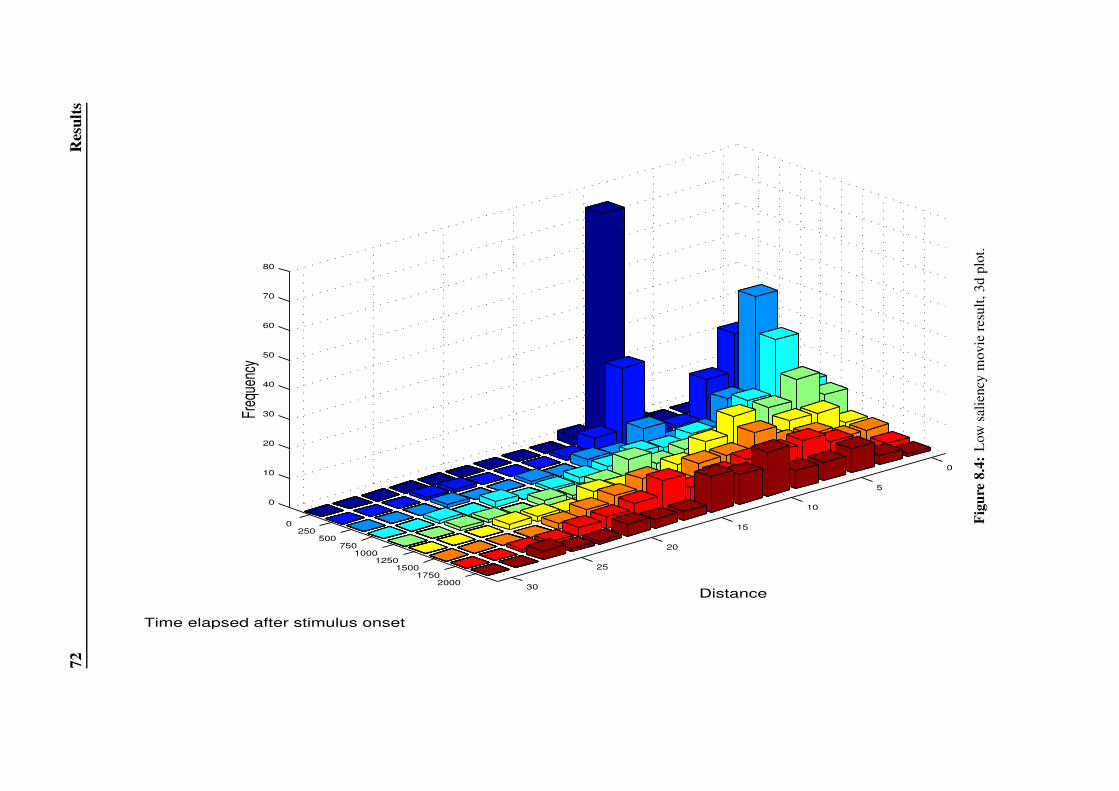
72R
esul
ts
0 250
500 750
10001250
15001750
2000
0
5
10
15
20
25
30
0
10
20
30
40
50
60
70
80
Distance
Time elapsed after stimulus onset
Freq
uenc
y
Figu
re8.
4:L
owsa
lienc
ym
ovie
resu
lt,3d
plot
.
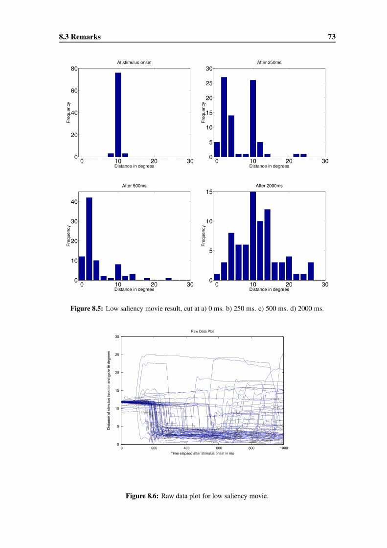
8.3 Remarks 73
0 10 20 300
20
40
60
80At stimulus onset
Distance in degrees
Freq
uenc
y
0 10 20 300
5
10
15
20
25
30After 250ms
Distance in degrees
Freq
uenc
y
0 10 20 300
10
20
30
40
After 500ms
Distance in degrees
Freq
uenc
y
0 10 20 300
5
10
15After 2000ms
Distance in degrees
Freq
uenc
y
Figure 8.5: Low saliency movie result, cut at a) 0 ms. b) 250 ms. c) 500 ms. d) 2000 ms.
0
5
10
15
20
25
30
0 200 400 600 800 1000
Dis
tanc
e of
stim
ulus
loca
tion
and
gaze
in d
egre
es
Time elapsed after stimulus onset in ms
Raw Data Plot
Figure 8.6: Raw data plot for low saliency movie.
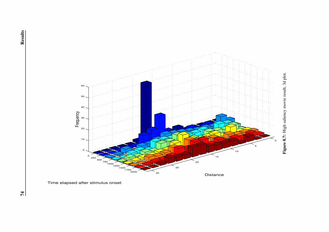
74R
esul
ts
0 250
500 750
10001250
15001750
2000
0
5
10
15
20
25
30
0
10
20
30
40
50
60
Distance
Time elapsed after stimulus onset
Freq
uenc
y
Figu
re8.
7:H
igh
salie
ncy
mov
iere
sult,
3dpl
ot.

8.3 Remarks 75
0 10 20 300
10
20
30
40
50
60At stimulus onset
Distance in degrees
Freq
uenc
y
0 10 20 300
5
10
15
20
25After 250ms
Distance in degrees
Freq
uenc
y
0 10 20 300
2
4
6
8
10After 500ms
Distance in degrees
Freq
uenc
y
0 10 20 300
2
4
6
8
After 2000ms
Distance in degrees
Freq
uenc
y
Figure 8.8: High saliency movie result, cut at a) 0 ms. b) 250 ms. c) 500 ms. d) 2000 ms.
0
5
10
15
20
25
30
35
40
0 200 400 600 800 1000
Dis
tanc
e of
stim
ulus
loca
tion
and
gaze
in d
egre
es
Time elapsed after stimulus onset in ms
Raw Data Plot
Figure 8.9: Raw data plot for high saliency movie.

76R
esul
ts
0 250
500 750
10001250
15001750
2000
0
5
10
15
20
25
30
0
5
10
15
20
25
30
35
Distance
Time elapsed after stimulus onset
Freq
uenc
y
Figu
re8.
10:
Res
ultf
orhi
ghsa
lienc
ym
ovie
whe
reth
est
imul
iwer
eno
tdra
wn.
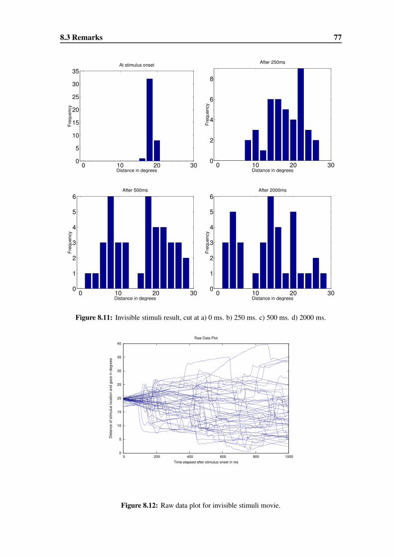
8.3 Remarks 77
0 10 20 300
5
10
15
20
25
30
35At stimulus onset
Distance in degrees
Freq
uenc
y
0 10 20 300
2
4
6
8
After 250ms
Distance in degrees
Freq
uenc
y
0 10 20 300
1
2
3
4
5
6After 500ms
Distance in degrees
Freq
uenc
y
0 10 20 300
1
2
3
4
5
6After 2000ms
Distance in degrees
Freq
uenc
y
Figure 8.11: Invisible stimuli result, cut at a) 0 ms. b) 250 ms. c) 500 ms. d) 2000 ms.
0
5
10
15
20
25
30
35
40
0 200 400 600 800 1000
Dis
tanc
e of
stim
ulus
loca
tion
and
gaze
in d
egre
es
Time elapsed after stimulus onset in ms
Raw Data Plot
Figure 8.12: Raw data plot for invisible stimuli movie.

78R
esul
ts
0 250
500 750
10001250
15001750
2000
0
5
10
15
20
25
30
0
1
2
3
4
5
6
7
8
Distance
Time elapsed after stimulus onset
Freq
uenc
y
Figu
re8.
13:
Res
ultf
orm
ediu
msa
lienc
ym
ovie
inhi
ghre
solu
tion.

8.3 Remarks 79
0 10 20 300
2
4
6
8At stimulus onset
Distance in degrees
Freq
uenc
y
0 10 20 300
0.5
1
1.5
2
2.5
3After 250ms
Distance in degrees
Freq
uenc
y
0 10 20 300
0.5
1
1.5
2
2.5
3After 500ms
Distance in degrees
Freq
uenc
y
0 10 20 300
0.5
1
1.5
2
2.5
3After 2000ms
Distance in degrees
Freq
uenc
y
Figure 8.14: High resolution, medium saliency result, cut at a) 0 ms. b) 250 ms. c) 500 ms. d)2000 ms.
0
5
10
15
20
25
30
0 200 400 600 800 1000
Dis
tanc
e of
stim
ulus
loca
tion
and
gaze
in d
egre
es
Time elapsed after stimulus onset in ms
Raw Data Plot
Figure 8.15: Raw data plot for high resolution, medium saliency movie.

80 Results
the first 100 ms of all plots. This is because we have discarded those stimuli that were
shorter than 100 ms. Stimuli were switched off when either gaze came closer than 8° to the
stimulus location or a saccade was detected. In the first 100 ms, a saccadic eye movement
must have been initiated prior to stimulus onset because of the minimal reaction time for
a saccade. Therefore, the data for these stimuli are not presented.

C H A P T E R 9
Discussion
It is fascinating to recognize how limited our mental capacity for information processing
is. The brain has found ingenious ways to give us the impression that we have full control
over our visual world at all times. But already at the anatomical level of the visual system,
we have seen that only a very small part of the visual field is processed in full detail. This
limitation is compensated for by several jump-like eye movements per second, so that the
important parts of the visual world are constantly scanned.
The decision of what the important parts of the visual world actually are is made by
attention. There exists a vast body of literature on attention, so we could probably only
give a glimpse on this exciting subject. But we have seen that attention is strongly limited
as well. Major changes to a visual scene, or even to objects of the real world, can go
unnoticed if the temporal transient is masked that is normally used by the brain to detect
such a change. Also, people sometimes fail to detect clearly visible objects when their
attention is absorbed by a task that does not include active search for such an object.
It is obvious that these limits can have severe consequences. For example, while driving
cars or monitoring dangerous machinery, just by blinking people are rendered blind for
potentially important changes about 20-30 times a minute. Being engaged in attention-
consuming tasks such as a conversation also reduces the capacity to process potentially
important visual input.
Therefore, it is desirable to develop systems that are adapted to this limited capacity and
that can help to attenuate these limits.
As of now, there still exists no way to record what a person is attending to, but gaze can be
measured reliably today. Although gaze and attention cannot be equated, there is a strong

82 Discussion
relationship between their underlying mechanisms. Attention is thought to precede eye
movements, so that we can assume that when a saccade is made to a location, this location
has also been attended to.
This does only guarantee that attention is paid to a specific location, but not that the correct
aspect of a scene at that location is encoded. Nevertheless, we believe that guidance of eye
movements is an important first step towards systems that help to overcome the limits of
human attention. To understand aspect-oriented attention, we probably need a full theory
of how the brain in general works, a goal that still lies in the distant future.
In this thesis, we have presented a system that can influence the eye movements of ob-
servers while watching dynamic natural scenes. It is important to point out that the results
we have given in chapter 8 are only preliminary. The emphasis of this thesis was on
the technical issues of building a gaze-contingent system that can display and manipulate
high resolution image sequences with a mean latency from the onset of an eye movement
to a change on the screen of less than 30 ms.
Real-time high resolution image processing at a refresh rate of 150 Hz is still a hard task
even for the fastest personal computers available today. Therefore, we carefully had to
select hardware components and software libraries that were suitable for this task. The
system software design was also optimized towards a minimum latency which included
writing of native assembly code and usage of today’s processor’s multi-processing ca-
pabilities. Finally, visual inspection of the high system dynamics was impossible. We
therefore had to implement technical means to verify the dynamics of our system.
Despite the emphasis on the technical issues, from our preliminary results we may hy-
pothesize that there is an effect on eye movements indeed, and that the strength of this
effect depends on the underlying image sequence.
To fully validate the results we have obtained, a more systematic testing of parameters
such as stimulus distance or size with a higher number of subjects would be required.
But we believe we can already identify some shortcomings of the current approach and
discuss where future work ought to be directed.
Two major issues have not been addressed within the presented experiments. First, in an
optimal system, the observers should not become aware of the fact that their scan path is
guided at all. If they become aware of this, they might choose to ignore the stimulation
Discussion 83
and actively suppress it. We have not implemented any measurements for the detection of
stimuli because that might have introduced an active search for them, which is detrimental
to the aim of the experiment. Nevertheless, verbal reports after experiments hint to a
detection of some, but not all stimuli. This is interesting because this means that subjects
could probably infer that more stimuli were to come, but they still reacted to them.
Generally, the experimental setup is still not well-suited for subjects not to notice any
stimulation. Their heads are fixated in an uncomfortable chin-rest, the movies shown are
probably fairly boring, and the frequency of stimulation is very high. Thus, attention
in some form, either suppressing or enhancing, is likely to be deployed to the fact that
some stimulation will take place. In a real application, only seldom interaction with
the user might be required. Especially if a less obtrusive method of eye-tracking may
become available, the feeling of being monitored in an experiment may diminish. Also, a
gradual increase in stimulus strength until a reaction is provoked might lower awareness
of stimulation as well.
The second issue is that the current stimulation does not exploit the underlying image
sequence as well as the previous scan path to their full extent. The mean spatio-temporal
curvature was used to model more probable saccade endpoints, but in one scale and with
a very simple thresholding rule only. Refined models should take into account larger
regions around the stimulus location, so that for example the velocity of a moving stimulus
is increased when there is already a high amount of optical flow in the vicinity. Also, a
history of past eye movements could help to better determine appropriate stimulation. For
example, a smooth pursuit eye movement could show that the observer is actively tracking
an object, so that stimulus strength probably needs to be higher than for a fixation.
Finally, we believe that the subject of gaze-contingent stimulation in natural dynamic
scenes opens up a wide field of applications. First, gaze-contingent experiments may al-
low to gain more insight into attentional processes. In the future, we also expect systems
to become available that help humans to enhance their information processing capabili-
ties.

Bibliography
[Ade87] George Adelman, editor. Encyclopedia of neuroscience. Birkhauser Boston,
1987.
[BB85] C L Baker and O J Braddick. Eccentricity-dependent scaling of the limits
of short-range motion perception. Vision Research, 25:803–12, 1985.
[Bec76] W Becker. Do correction saccades depend exclusively on retinal feed-
back? A note on the possible role of non-retinal feedback. Vision Research,
16:425–7, 1976.
[Bec91] W Becker. Saccades. In R H S Carpenter, editor, Vision & Visual Dysfunc-
tion Vol 8: Eye Movements, pages 95–137. CRC Press, 1991.
[BHC+99] Theodore T Blackmon, Yeuk Fai Ho, Dimitri A Chernyak, Michela Az-
zariti, and Lawrence W Stark. Dynamic scanpaths: eye movement analysis
methods. In Proc SPIE Conf, 1999.
[BHS75] B Bridgeman, D Hendry, and L Stark. Failure to detect displacement of the
visual world during saccadic eye movements. Vision Research, 15(6):719–
22, 1975.
[BJ79] W Becker and R Jurgens. An analysis of the saccadic system by means of
double step stimuli. Vision Research, 19:967–83, 1979.
[BKBM04] Martin Bohme, Christopher Krause, Erhardt Barth, and Thomas Martinetz.
Eye movement predictions enhanced by saccade detection. In Proc of Brain
Inspired Cognitive Systems, 2004. (submitted).
[Bri00] Bruce Bridgeman. Workshop Notes: The Two Visual Systems and their
Interactions. http://www.ircs.upenn.edu/cogsci2000/Bridgeman.pdf, 2000.
Bibliography 85
[Bro58] D E Broadbent. Perception and communication. Pergamon Press, 1958.
[CMCRI95] C Currie, G W McConkie, L A Carlson-Radvansky, and D E Irwin. Main-
taining visual stability across saccades: Role of the saccade target object,
1995.
[dB97] Bart de Bruyn. Blending Transparent Motion Patterns in Peripheral Vision.
Vision Research, 37(5):645–8, 1997.
[Del98] E B Delabarre. A method of recording eye-movements. American Journal
of Psychology, 9(4):572–4, 1898.
[Den91] Daniel C Dennett. Consciousness Explained. Little, Brown and Co., 1991.
[DV00] Andrew Duchowski and Roel Vertegaal. Eye-Based Interaction in Graph-
ical Systems: Theory and Practice. SIGGRAPH 2000 Course Notes.
http://www.vr.clemson.edu/eyetracking/sigcourse, 2000.
[EJ86] C W Eriksen and J D St James. Visual attention within and around the
field of focal attention: A zoom lens model. Perception and Psychophysics,
40:225–40, 1986.
[EOT] OpenTop Cross-Platform Library. http://www.elcel.com/products/opentop.
[FG03] John M Findlay and Ian D Gilchrist. Visual Attention: The Active Vision
Perspective. In John M Findlay and Iain D Gilchrist, editors, Active Vision:
The Psychology of Looking and Seeing, pages 85–106. Oxford University
Press, 2003.
[FLT] Fast Lightning Toolkit. http://www.fltk.org.
[FR86] B Fischer and E Ramsperger. Human express saccades: effects of random-
ization and daily practice. Experimental Brain Research, 64:569–78, 1986.
[Fre53] R S French. The discrimination of dot patterns as a function of number and
average separation of dots. Journal of Experimental Psychology, 46:1–9,
1953.
[Gro] Independent JPEG Group. http://www.ijg.org.

86 Bibliography
[Hai91] R F Haines. A breakdown in simultaneous information processing. In
G Obrecht and L W Stark, editors, Presbyopia research: From molecular
biology to visual adaptation, pages 171–5. Plenum Press, 1991.
[HBT+02] Mary M Hayhoe, Dana H Ballard, Jochen Triesch, Hiroyuki Shinoda, Pilar
Aivar, and Brian Sullivan. Vision in natural and virtual environments. In
Eye Tracking Research & Application, pages 7–13, 2002.
[Hec80] J Hecker. Der Einfluss stimulierender Substanzen auf die sakkadischen Au-
genbewegungen. PhD thesis, Universitat Ulm, 1980.
[Hof98] James E Hoffman. Attention and eye movements, 1998.
[HSA92] Selim S Hacisalihzade, Lawrence W Stark, and John S Allen. Visual Per-
ception and Sequences of Eye Movement Fixations: A Stochastic Mod-
eling Approach. IEEE Transactions on Systems, Man, and Cybernetics,
22(3):474–81, 1992.
[HW85] O Hikosaka and R H Wurtz. Modification of saccadic eye movements by
GABA-related substances. Journal of Neurophysiology, 53:266–309, 1985.
[IIP] Intel Integrated Performance Primitives Library, Image Processing Samples.
http://www.intel.com/software/products/ipp/samples.htm.
[Ins03] SensoMotoric Instruments. iViewX Highspeed Users’ Manual, 2003.
[Jam90] William James. The Principles of Psychology. Henry Holt, 1890. On-line
edition at http://psychclassics.yorku.ca/James/Principles.
[Jav78] E Javal. Essai sur la physiologie de la lecture. Annales d’Oculistique, 79:97,
1878.
[JHG99] Bernd Jaehne, H Haußecker, and P Geißler, editors. Handbook of Computer
Vision and Applications. Academic Press, 1999.
[Jon81] J Jonides. Voluntary versus automatic control over the mind’s eye’s move-
ment. In J B Long and A D Baddeley, editors, Attention and performance,
volume IX, pages 187–203. Lawrence Erlbaum Associates Inc., 1981.

Bibliography 87
[KSJ95] Eric R Kandel, James H Schwartz, and Thomas M Jessell, editors. Essen-
tials of neural science and behavior. Prentice Hall International, 1995.
[Lat62] P Latour. Visual thresholds during eye movements. Vision Research, 2:261–
2, 1962.
[Leh03] Wolfgang Lehmann. TTL IO. Personal communication, 10 2003.
[LG03] Casimir J H Ludwig and Iain D Gilchrist. Goal-driven modulation of ocu-
lomotor capture. Perception & Psychophysics, 65(8):1243–51, 2003.
[LJI72] H W Leibowitz, C A Johnson, and E Isabelle. Peripheral motion detection
and refractive error. Science, 177:1207–8, 1972.
[LZ99] R John Leigh and David S Zee, editors. The Neurology of Eye Movements.
Oxford University Press, 1999.
[Mar82] David Marr. Vision. W H Freeman, 1982.
[MB00] Cicero Mota and Erhardt Barth. On the uniqueness of curvature features. In
G Baratoff and H Neumann, editors, Dynamische Perzeption, volume 9 of
Proceedings in Artifical Intelligence, pages 175–8. 2000.
[MD85] J Moran and R Desimone. Selective attention gates visual processing in the
extrastriate cortex. Science, 229:782–4, 1985.
[MDSB04] Cicero Mota, Michael Dorr, Ingo Stuke, and Erhardt Barth. Categorization
of Transparent-Motion Patterns Using the Projective Plane. International
Journal of Computer and Information Science, 2004. (submitted).
[MR98] A Mack and I Rock. Inattentional Blindness. MIT Press, 1998.
[MT98] Bruce Milliken and Steven P Tipper. Attention and Inhibition. In Harold
Pashler, editor, Attention, chapter 5, pages 191–221. Psychology Press,
1998.
[NB75] U Neisser and R Becklen. Selective looking: Attending to visually specified
events. Cognitive Psychology, 7:480–94, 1975.
[Nei67] U Neisser. Cognitive psychology. New York: Appleton, 1967.

88 Bibliography
[ODCR00] J K O’Regan, H Deubel, J J Clark, and R A Rensink. Picture changes
during blinks: looking without seeing and seeing without looking. Visual
Cognition, 7:191–212, 2000.
[OGE84] F P Ottes, J A M Van Gisbergen, and J J Eggermont. Metrics of saccade
responses to visual double stimuli: two different modes. Vision Research,
24:1169–74, 1984.
[ON01] J Kevin O’ Regan and Alva Noe. A sensorimotor account of vision and vi-
sual consciousness. Behavioral and Brain Sciences, 24(5):939–1011, 2001.
[ORC00] J K O’Regan, R A Rensink, and J J Clark. Change-blindness as a result of
’mudsplashes’. Nature, 398:34, 2000.
[Pas98] Harold Pashler, editor. Attention. Psychology Press, 1998.
[PB01] Christopher C Pack and Richard T Born. Temporal dynamics of a neural
solution to the aperture problem in visual area MT of macaque brain. Nature,
409:1040–2, 2001.
[Pos80] M I Posner. Orienting of attention. Quarterly Journal of Experimental
Psychology, 32:3–25, 1980.
[RRDU87] G Rizzolatti, L Riggio, I Dascola, and C Umilita. Reorienting attention
across the vertical and horizontal meridians: Evidence in favor of a premotor
theory of attention. Neuropsychologia, 25:31–40, 1987.
[RS04] Daniel C Richardson and Michael J Spivey. Eye-Tracking: Characteristics
and Methods. In G Wnek and G Bowlin, editors, Encyclopedia of Biomate-
rials and Biomedical Engineering. 2004. (Preprint).
[RSA92] J E Raymond, K L Shapiro, and K M Arnell. Temporary suppression of
visual processing in an RSVP task: An attentional blink? Journal of Ex-
perimental Psychology: Human Perception and Performance, 18:849–60,
1992.

Bibliography 89
[RZHB02] Rajesh P N Rao, Gregory J Zelinsky, Mary M Hayhoe, and Dana H Ballard.
Eye movements in iconic visual search. Vision Research, 42(11):1447–63,
2002.
[SC99] Daniel J Simons and Christopher F Chabris. Gorillas in our midst: sustained
inattentional blindness for dynamic events. Perception, 28:1059–74, 1999.
[SD00] Werner X Schneider and Heiner Deubel. Selection-for-perception and
selection-for-spatial-motor-action are coupled by visual attention: a review
of recent findings and new evidence from stimulus-driven saccade control.
In Wolfgang Prinz and Bernhard Hommel, editors, Common Mechanisms in
Perception and Action, pages 609–27. Oxford University Press, 2000.
[Sim96] Daniel J Simons. In sight, out of mind: When object representations fail.
Psychological Science, 7(5):301–5, 1996.
[Sim00] Daniel J Simons. Current approaches to change blindness. Visual Cognition,
7(1-3):1–15, 2000.
[SL97] Daniel J Simons and D T Levin. Change blindness. Trends in Cognitive
Science, 1(7):261–7, 1997.
[Sto96] Petra Stoerig. Varieties of vision: from blind responses to conscious recog-
nition. Trends in Neuroscience, 19(9):401–6, 1996.
[Tex01] Texas Advanced Optoelectronics Solutions. TAOS TSL250R Data Sheet,
2001.
[TSHB02] Jochen Triesch, Brian T Sullivan, Mary M Hayhoe, and Dana H Ballard.
Saccade contingent updating in virtual reality. In Eye Tracking Research &
Application, pages 95–102, 2002.
[Wol98] Jeremy M Wolfe. Visual Search. In Harold Pashler, editor, Attention, pages
13–73. Psychology Press, 1998.
[WW73] R E Walley and T D Weiden. Lateral inhibition and cognitive masking: A
neuropsychologial theory of attention. Psychological Review, 80:284–302,
1973.

90 Bibliography
[Yan98] Steven Yantis. Control of Visual Attention. In Harold Pashler, editor, Atten-
tion, chapter 6, pages 223–56. Psychology Press, 1998.
[Yar67] A L Yarbus. Eye Movements and Vision. Plenum Press, 1967.