Effects: Example 1 20 15 10 5 Low High Variable 2.
69
-
Upload
alyson-harrington -
Category
Documents
-
view
218 -
download
0
Transcript of Effects: Example 1 20 15 10 5 Low High Variable 2.


Effects: Example 1
20
15
10
5
Low High
Variable 2

Effects: Example 1
20
15
10
5
Low High
Variable 2
Variable 1 (Low)

Effects: Example 1
20
15
10
5
Low High
Variable 2
Variable 1(High)
Variable 1 (Low)

20
15
10
5
Low High
Variable 2
Effects: Example 2
20
15
10
5
Low High
Variable 2
Effects: Example 2
Variable 1 (Low)

20
15
10
5
Low High
Variable 2
Effects: Example 2
Variable 1 (High)
Variable 1 (Low)

Interaction EffectsDefined: dependent variable effects from
independent variables taken together
Forms: Ordinal
(in the same direction as the main effects of variables involved)
Disordinal
(not in the same direction as the main effects of
the variables involved)

Interpreting Ordinal Interactions
• acceptable to look at the independent variables separately
• permissible to interpret main effects for independent variables involved in the interaction
20
15
10
5
Low High
Variable 1
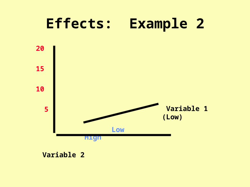
Effects: Example 3

20
15
10
5
Low High
Variable 1
Effects: Example 3
Variable 2 (Low)
20
15
10
5
Low High
Variable 1
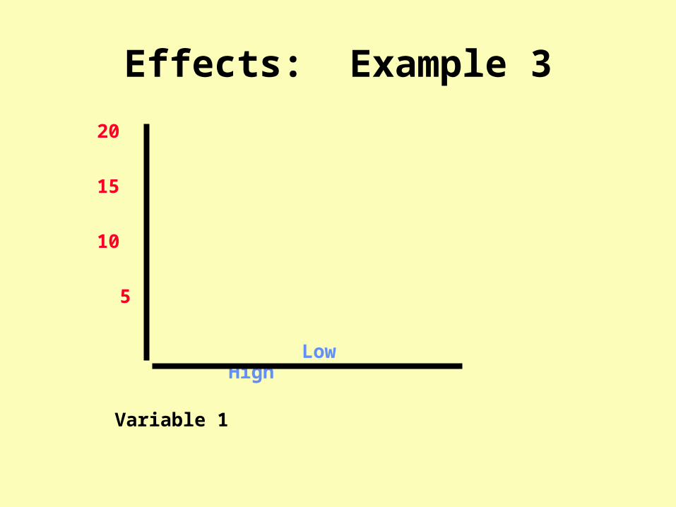
Effects: Example 3
Variable 2 (Low)
Variable 2 (High)

Interpreting Disordinal Interactions
• must look at both independent variables together
• not permissible to interpret main effects for independent variables involved in the interaction

20
15
10
5
Low High
Variable 2
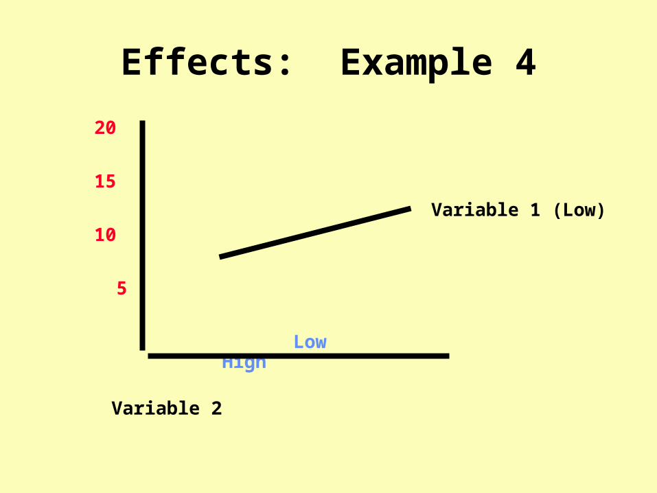
Effects: Example 4
20
15
10
5
Low High
Variable 2
Effects: Example 4
Variable 1 (Low)

20
15
10
5
Low High
Variable 2
Effects: Example 4
Variable 1 (High)
Variable 1 (Low)

20
15
10
5
Low High
Variable 2
Effects: Example 5

20
15
10
5
Low High
Variable 2
Effects: Example 5
Variable 1 (Low)

20
15
10
5
Low High
Variable 2
Effects: Example 5
Variable 1 (Low)
Variable 1 (High)

20
15
10
5
Low High
Variable 2
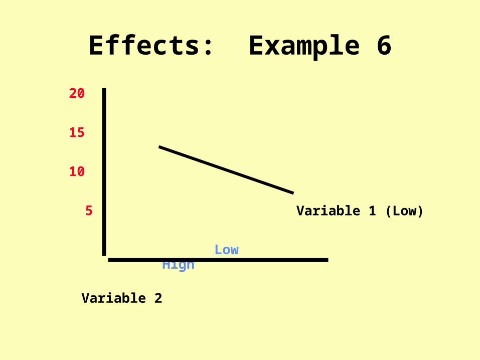
Effects: Example 6
20
15
10
5
Low High
Variable 2
Effects: Example 6
Variable 1 (Low)

20
15
10
5
Low High
Variable 2
Effects: Example 6
Variable 1 (High) Variable 1 (Low)
• Computing Sampling Error• Measurement• Hypothesis Testing
Decisions• Types of Statistical tests

Confidence Intervals
for Proportions
Slide 11.1A

Confidence Intervals
for Proportions
Slide 11.1B
90% CI = 1.645*p *(1- p)
sample size
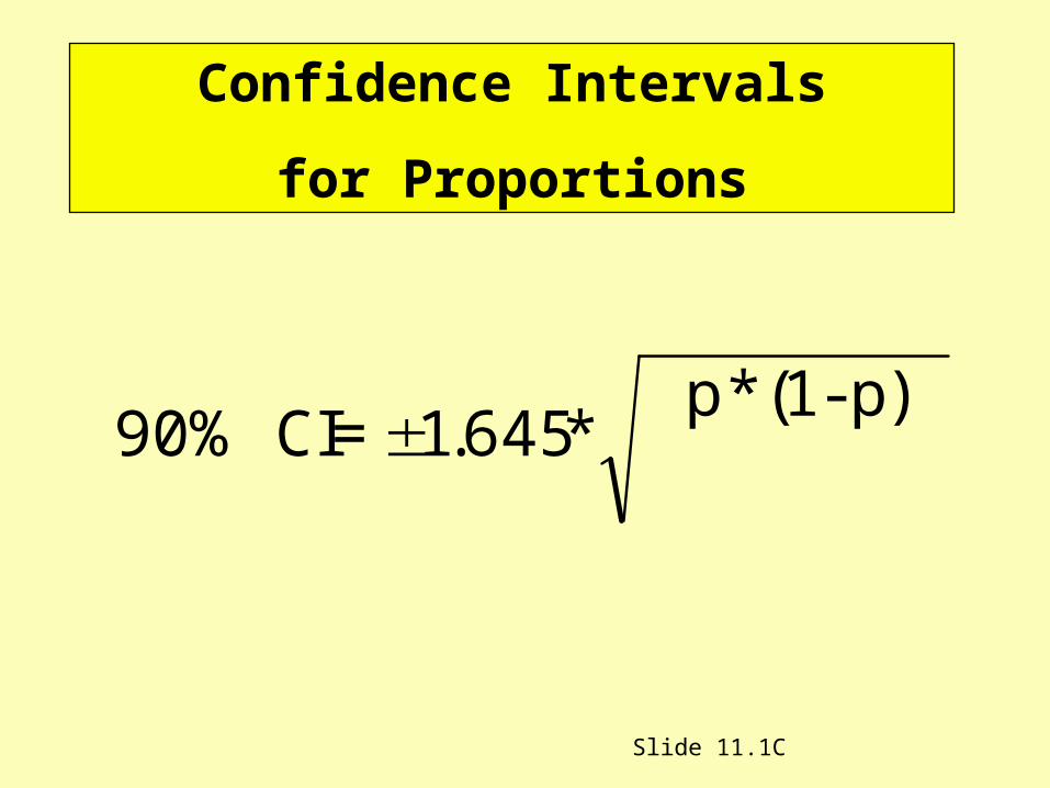
Confidence Intervals
for Proportions
Slide 11.1C

90% CI = 1.645*p *(1- p)
sample size
Confidence Intervals
for Proportions
Slide 11.1
90% CI = 1.645*p *(1- p)
sample size
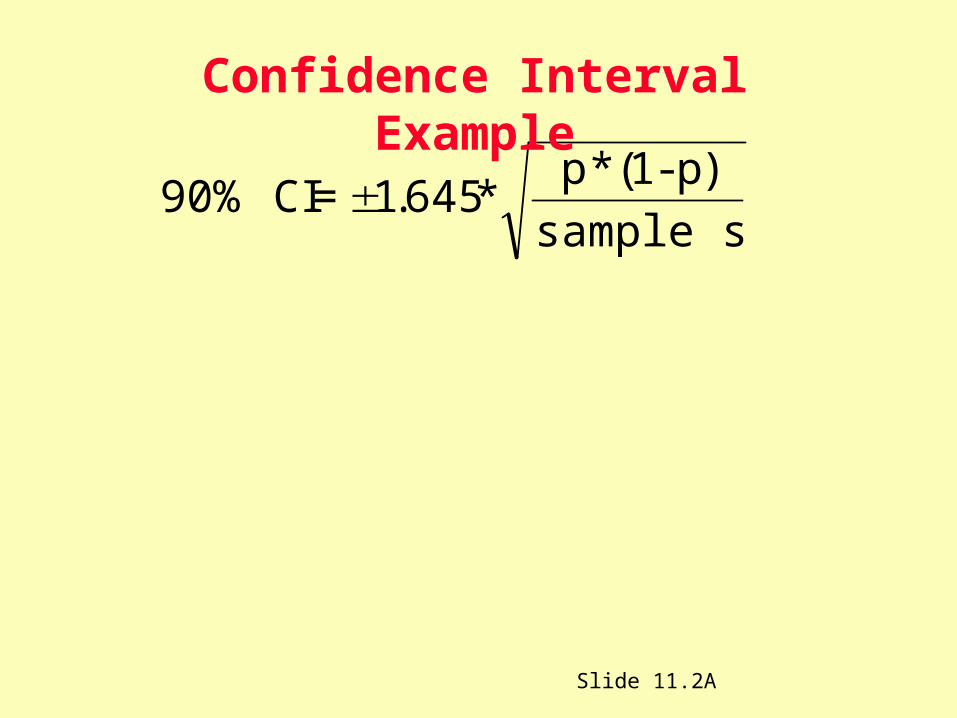
Confidence Interval Example
Slide 11.2A

90% CI = 1.645*p *(1- p)
sample size
90% CI = 1.645*.7*(1-.7)
10
Confidence Interval Example
Slide 11.2B

90% CI = 1.645*p *(1- p)
sample size
90% CI = 1.645*.7*(1-.7)
10
90% CI = 1.645*.21
10
Confidence Interval Example
Slide 11.2

90% CI = 1.645* .021
Slide 11.3A

90% CI = 1.645* .14
90% CI = 1.645* .021
Slide 11.3B

90% CI = .23
90% CI = 1.645* .14
90% CI = 1.645* .021
Slide 11.3C

90% CI = .23
90% CI = 1.645* .14
90% CI = 1.645* .021
One is 90% confident that the proportion of the population that is displeased is equal to .7 (seventy percent), plus or minus .23 (twenty-three percent)
Slide 11.3

Effects on Confidence Interval If:
• Sample size is increased to 100: .07
• Confidence Interval at 95%: .27
• Confidence Interval at 99%: .46
Slide 11.4
Selecting a Sample Size
• Study Objectives
• Time Limits
• Cost
• Data Analysis

• Computing Sampling Error• Measurement• Hypothesis Testing
Decisions• Types of Statistical tests

Nominal Level Measurement
• numbers used as ways to identify or name categories
• numbers do not indicate degrees of a variable but simple groupings of variables
• equivalent to qualitative data
Slide 8.1
Ordinal Level Measurement
• uses rank order to determine differences
• measures whether items are “greater than” or “less than” other items
• identifies relations of measured items to each other
Slide 8.2

Interval Level Measurement
• distances between measured items are identified by a matter of degree
• allows meaningful arithmetic to be applied
• measures whether items are “greater than” or “less than” other items
• permits identifying the ratio of intervals to each other
Slide 8.3
Ratio Level Measurement
• distances between measured items are identified by a matter of degree
– a true quantitative scale and includes an “absolute zero”
• allows meaningful arithmetic to be applied
• measures whether items are “greater than” or “less than” other items
• permits identifying the ratio of intervals to each other
Slide8.4

• Computing Sampling Error• Measurement• Hypothesis Testing
Decisions• Types of Statistical tests

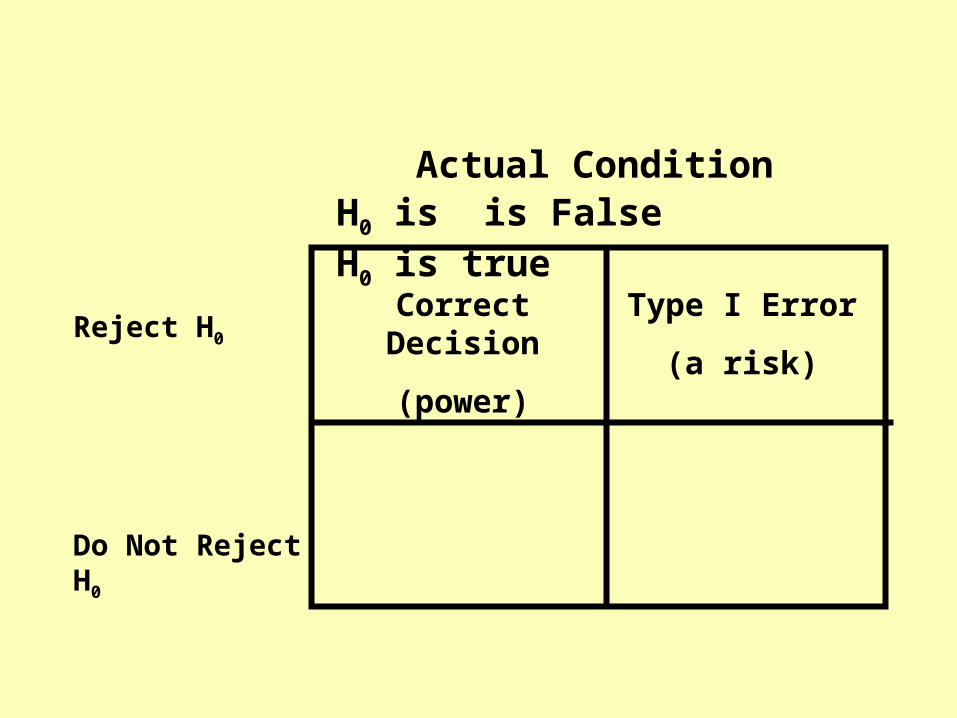
Actual ConditionH0 is is False H0 is true

Actual ConditionH0 is is False H0 is true
Reject H0
Do Not Reject H0

Actual ConditionH0 is is False H0 is true
Reject H0
Do Not Reject H0
Correct Decision
(power)
Actual ConditionH0 is is False H0 is true
Reject H0
Do Not Reject H0
Correct Decision
(power)
Type I Error
(a risk)

Actual ConditionH0 is is False H0 is true
Reject H0
Do Not Reject H0
Correct Decision
(power)
Type I Error
(a risk)
Type II Error
(b risk)

Actual ConditionH0 is is False H0 is true
Reject H0
Do Not Reject H0
Correct Decision
(power)
Type I Error
(a risk)
Type II Error
(b risk)Correct decision

• Computing Sampling Error• Measurement• Hypothesis Testing
Decisions• Types of Statistical tests

One Sample t Test
tX
s n
Slide 13.1
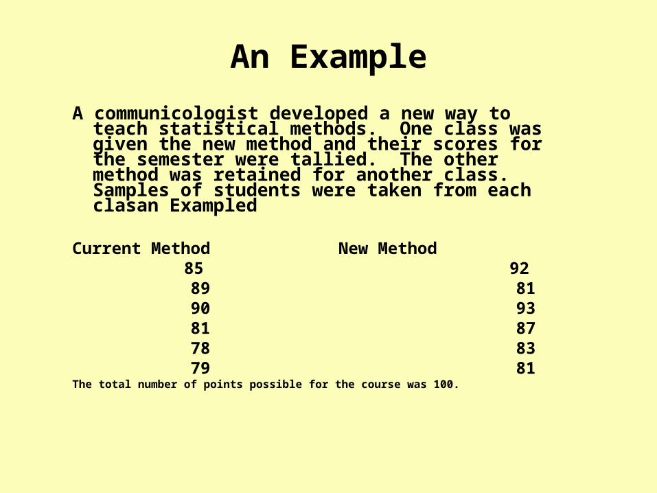
An Example
A communicologist developed a new way to teach statistical methods. One class was given the new method and their scores for the semester were tallied. The other method was retained for another class. Samples of students were taken from each clasan Exampled
Current Method New Method 85 92 89 81 90 93 81 87 78 83 79 81 The total number of points possible for the course was 100.

Null Hypothesis for Two Sample t Test
H0 : new current
Slide 13.2
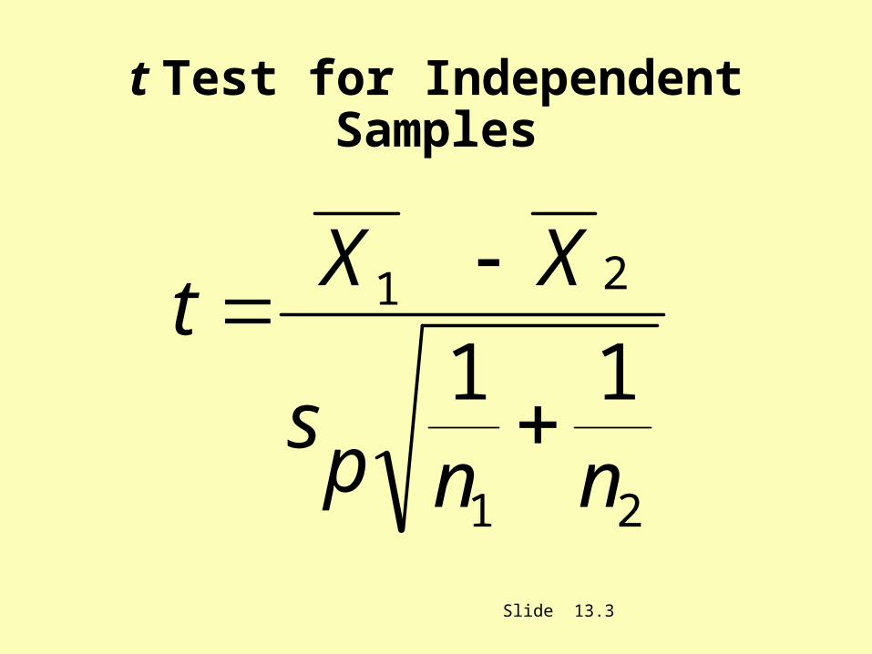
t Test for Independent Samples
tX X
sp n n
1 2
1 2
1 1
Slide 13.3

Finding the Critical Region of t
-2.228 2.228
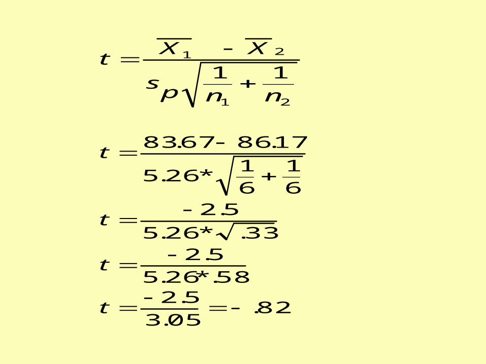
tX X
sp n n
1 2
1 2
1 1
t
t
t
t
83 67 86 17
5 2616
16
2 5
5 26 332 5
5 26 582 5
3 0582
. .
. *
.
. * ..
. *..
..
Agenda
• Hypothesis Testing Decisions
• t tests
•ANOVA• chi square

Comparing More thanTwo Means
Mean A Mean B Mean C
Slide 14.1
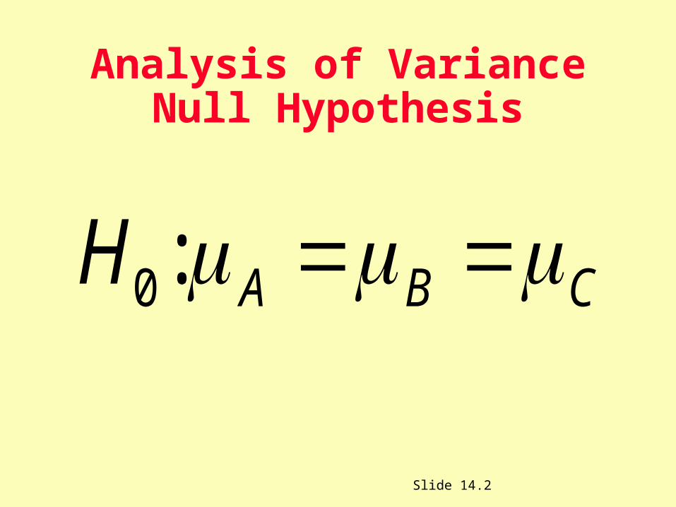
Analysis of VarianceNull Hypothesis
H A B C0:
Slide 14.2

Analysis of Variance
Slide 14.3A

18
40
62
60
Public Speaking
Take Don’t Take
international students
national students
Slide 14.6A
Chi Square Example

18
40
62
60
Public Speaking
Take Don’t Take
international students
national students
80
100
Slide 14.6B
Chi Square Example

18
40
62
60
Public Speaking
Take Don’t Take
international students
national students
80
100
58 122
Slide 14.6
Chi Square Example

18
40
62
60
Public Speaking
Take Don’t Take
international students
national students
80
100
58 122
25.52
Slide 14.7A
Chi Square Example
18
40
62
60
Public Speaking
Take Don’t Take
international students
national students
80
100
58 122
25.52
Slide 14.7B
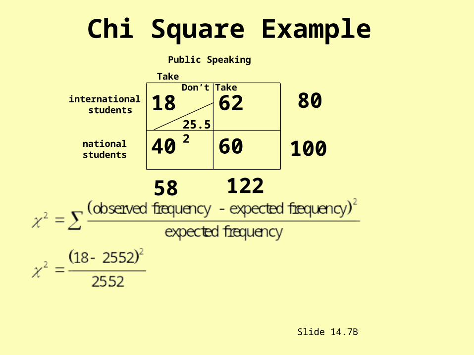
Chi Square Example

18
40
62
60
Public Speaking
Take Don’t Take
international students
national students
80
100
58 122
25.52
32.48
Slide 14.7C
Chi Square Example
18
40
62
60
Public Speaking
Take Don’t Take
international students
national students
80
100
58 122
25.52 53.68
32.48
Slide 14.7D
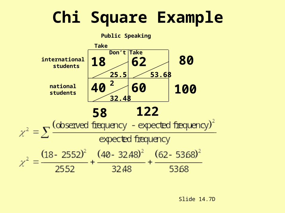
Chi Square Example

18
40
62
60
Public Speaking
Take Don’t Take
international students
national students
80
100
58 122
25.52 53.68
32.48 68.32
Slide 14.7E
Chi Square Example

2
2
2
2 2 2 2
2
18 2552
2552
40 32 48
32 48
62 5368
5368
60 68 32
68 322 22 174 129 101 6 26
observed frequency - expected frequency
expected frequency
.
.
.
.
.
.
.
.. . . . .
18
40
62
60
Public Speaking
Take Don’t Take
international students
national students
80
100
58 122
25.52 53.68
32.48 68.32
Slide 14.7F
Chi Square Example

2
2
2
2 2 2 2
2
18 2552
2552
40 32 48
32 48
62 5368
5368
60 68 32
68 322 22 174 129 101 6 26
observed frequency - expected frequency
expected frequency
.
.
.
.
.
.
.
.. . . . .
18
40
62
60
Public Speaking
Take Don’t Take
international students
national students
80
100
58 122
25.52 53.68
32.48 68.32
Slide 14.7
Chi Square Example