EFFECTIVENESS METHOD FOR HEAT AND MASS TRANSFER IN MEMBRANE HUMIDIFIERS

by

DAVID ERWIN KADYLAK

B.A.Sc., The University of Waterloo, 2006

A THESIS SUBMITTED IN PARTIAL FULFILLMENT OF THE REQUIREMENTS FOR THE DEGREE OF

MASTER OF APPLIED SCIENCE

in

The Faculty of Graduate Studies

(Mechanical Engineering)

THE UNIVERSITY OF BRITISH COLUMBIA

(Vancouver)

April 2009

© David Erwin Kadylak, 2009

ii

ABSTRACT

A thermodynamic model for use in predicting heat and water transfer across a

membrane in a membrane humidifier was created that could take into account fuel cell

operating conditions. Experiments were conducted to obtain the necessary information to

make the model complete, and also to validate its use over a range of temperatures and

flow rates.

The latent effectiveness and latent number of transfer units (ε-NTU) method for

mass transfer in membrane humidity exchangers was applied to PEMFC membrane

humidifiers to comprise the heat and mass transfer thermodynamic model. Two

limitations that cause deviations in the theoretical outlet conditions previously reported

were discovered: 1. using a constant enthalpy of vaporization derived from the reference

temperature in the Clausius-Clapeyron equation; and, 2. simplifying the relationship

between relative humidity and absolute humidity as linear. In the model presented here,

these limitations are alleviated by using an effective mass transfer coefficient Ueff. The

model was created in Mathcad and the constitutive equations are solved iteratively to find

the flux of water through the membrane.

The new procedure was applied to three types of membrane and compared to the

curves of εL and NTUL found using Zhang and Niu’s method, which is normally applied

to energy recovery ventilators (ERVs). For a 70°C isothermal case, a deviation in latent

effectiveness predictions was observed of 29% for Type-I membranes, 23% for linear-

type membranes, and 46% for Type-III membranes, as compared to the latent

effectiveness values obtained with the ERV method.

iii

Experiments were conducted on a commercially available fuel cell humidifier to

determine which parameters could be removed from a full-factorial experimental matrix.

It was discovered that pressure had a lower effect on water transport than temperature

over the practical operating range of fuel cell systems, so pressure effects were neglected

throughout the study. The focus of the study was then on the effect of overall

temperature. Furthermore, it was determined that water recovery ratio is the best

performance metric because it takes into account the water supplied to the humidifier.

Two different membranes were characterized to incorporate into the

thermodynamic model. The first, used as a baseline, was a porous polymer membrane

with a hydrophilic additive. The second membrane was a competing novel ionic

membrane. Both membranes showed similar behavior, with low water uptake profiles at

relative humidities less than 80%, and a steep increase in water uptake after 80% relative

humidity. The porous membrane exhibited greater maximum sorption than the ionic

membrane.

Experiments were conducted with samples of the porous and ionic membrane in a

single cell humidifier at isothermal conditions at temperatures of 25°C, 50°C, and 75°C.

The ionic membrane showed greater water transfer over the range of laminar flows

investigated. The ionic membrane’s water recovery was almost unaffected by flow rate;

whereas the porous membrane displayed a decrease in water recovery as flow rate

increased. Finally, the model was correlated with the experimental data by obtaining a

corresponding diffusion coefficient for each membrane over the range of temperatures

tested.

Keywords: humidifier, membrane, fuel cell, effectiveness, moisture transfer, NTU

iv

TABLE OF CONTENTS

ABSTRACT ...................................................................................................................ii

TABLE OF CONTENTS ............................................................................................. iv

LIST OF TABLES ....................................................................................................... vi

LIST OF FIGURES..................................................................................................... vii

LIST OF SYMBOLS AND ABBREVIATIONS ......................................................... ix

ACKNOWLEDGEMENTS ......................................................................................... xi

DEDICATION ............................................................................................................xiii

1. INTRODUCTION ................................................................................................... 1

1.1. WATER MANAGEMENT IN FUEL CELLS................................................................ 1

1.2. ACTIVE VS. PASSIVE METHODS .......................................................................... 4

1.3. PERFORMANCE METRICS ................................................................................... 7

1.3.1. Measures based on supplied humidity ................................................... 7

1.3.2. Absolute measures .............................................................................. 10

1.3.3. Measures based on available humidity ................................................ 10

1.4. VARIABLES AND PARAMETERS AFFECTING WATER TRANSFER ........................... 12

1.4.1. Plate geometry .................................................................................... 12

1.4.2. Membrane properties .......................................................................... 13

1.4.3. Flow conditions .................................................................................. 13

1.5. THESIS OBJECTIVE........................................................................................... 14

1.6. THESIS OVERVIEW........................................................................................... 18

2. EXPERIMENTS .................................................................................................... 20

2.1. EXPERIMENTAL SETUP .................................................................................... 20

2.1.1. Test station ......................................................................................... 20

2.1.2. Humidifier .......................................................................................... 21

2.1.3. Maintaining isothermal conditions ...................................................... 23

2.2. EVALUATION OF PERFORMANCE MEASURES ..................................................... 23

2.3. PARAMETER EFFECT STUDY ............................................................................. 26

2.4. MEMBRANE CHARACTERIZATION .................................................................... 30

2.4.1. Solution-diffusion and sorption curves ............................................... 30

2.4.2. Water uptake of a hydrophilic-impregnated polymer .......................... 32

2.4.3. Water uptake of a perfluorinated composite membrane ....................... 34

2.4.4. Comparison of the porous and ionic membranes ................................. 35

2.5. EXPERIMENTAL DESIGN................................................................................... 36

2.5.1. Test matrix and conditions .................................................................. 37

2.6. MEMBRANE RESULTS AND DISCUSSION ............................................................ 40

3. HEAT AND WATER TRANSFER MODEL ....................................................... 43

3.1. HEAT TRANSFER USING THE EFFECTIVENESS METHOD ...................................... 43

v

3.2. THE CHILTON-COLBURN ANALOGY FOR MASS TRANSFER ................................. 44

3.3. CURRENT LATENT EFFECTIVENESS DERIVATIONS ............................................. 47

3.4. CURRENT LIMITATIONS OF ε-NTU METHOD FOR MASS TRANSFER ..................... 51

3.4.1. Use of the Clausius-Clapeyron saturation vapor pressure equation ...... 52

3.4.2. Correlation between absolute humidity and relative humidity ............. 53

3.5. A NEW APPROACH TO USING LATENT EFFECTIVENESS ....................................... 55

3.6. RESULTS OF COMPARISON TO PREVIOUS EFFECTIVENESS METHOD ..................... 58

3.7. EXPERIMENTAL VALIDATION OF MODEL........................................................... 61

4. CONCLUSIONS .................................................................................................... 64

4.1. FUTURE WORK ................................................................................................ 67

REFERENCES ............................................................................................................ 68

APPENDIX: DOCUMENTED MATHCAD MODEL ............................................... 72

vi

LIST OF TABLES

Table 1.1: Dependence of humidifier geometry characteristics on performance ....................................... 12

Table 1.2: Dependence of membrane properties on humidifier performance ............................................ 13

Table 1.3: Dependence of stream flow conditions on humidifier performance ......................................... 13

Table 1.4: Summary table comparing relevant past research from Zhang and Niu [29,31,32], Huizing [25],

Cave [26], Chen and Peng [19,22], Monroe and Romero [24], Park, Choe, Choi [21], and Park

and Oh [20,33] ................................................................................................................... 17

Table 2.1: Experimental matrix for temperature-dependence testing........................................................ 27

Table 2.2: Experimental matrix for pressure-dependence testing ............................................................. 28

Table 2.3: Experimental testing matrix ................................................................................................... 39

Table 3.1: Summary of parameters used in humidifier model comparisons .............................................. 58

Table 3.2: Comparison based on methodology of latent NTU and latent effectiveness for 0% dry inlet RH

.......................................................................................................................................... 61

vii

LIST OF FIGURES

Figure 1.1: Effect of reactant stream humidity on PEM fuel cell voltage output; adapted from [5] ............. 1

Figure 1.2: Balance of plant of humidifier and fuel cell system ................................................................. 3

Figure 1.3: Schematic of layered humidifier plates in cross-flow arrangement .......................................... 7

Figure 1.4: Overview structure of thesis ................................................................................................. 19

Figure 2.1: Experimental setup of test station in line with test humidifier ................................................ 21

Figure 2.2: Experimental single cell humidifier with installed ports ........................................................ 22

Figure 2.3: Water transfer as operating temperature is changed ............................................................... 24

Figure 2.4: Water transfer as dry stream pressure is changed .................................................................. 26

Figure 2.5: Effect on water transfer of changing dry inlet temperature .................................................... 27

Figure 2.6: Effect on water transfer of changing dry out backpressure, low total pressure ........................ 28

Figure 2.7: Effect on water transfer of changing dry out backpressure, high total pressure ....................... 29

Figure 2.8: Sorption isotherm at 25°C of hydrophilic additive-impregnated porous polymer membrane... 33

Figure 2.9: Sorption isotherm at 25°C of ionic perfluorinated composite membrane ................................ 35

Figure 2.10: Comparison of sorption isotherm at 25°C of a porous and an ionic membrane ..................... 36

Figure 2.11: Experimental results for porous polymer membrane E, at ♦ Tiso = 25°C, ● 50°C, ■ 75°C ..... 40

Figure 2.12: Experimental results for composite ionic membrane D, at ♦ Tiso = 25°C, ● 50°C, ■ 75°C..... 41

Figure 2.13: Comparison of water recovery ratio between two membranes, at ♦ Tiso = 25°C, ● 50°C, ■ 75°C .................................................................................................................................. 42

Figure 3.1: Variation in Lewis number term with relative humidity at different temperatures .................. 46

Figure 3.2: Comparison of saturated vapor pressure from four different equations .................................. 52

Figure 3.3: Magnitude of second term compared to first on right hand side of Eqn. (50).......................... 54

Figure 3.4: Procedure for solving humidifier outlet conditions ................................................................ 57

Figure 3.5: Variation of NTUL with inlet relative humidity for constant NTU: a) Type-I membrane (C =

0.1); b) linear-type membrane (C = 1); c) Type-III membrane (C = 10) ............................... 59

Figure 3.6: Latent effectiveness for constant NTU: a) Type-I membrane (C = 0.1); b) linear-type

membrane (C = 1); c) Type-III membrane (C = 10) ............................................................. 60

Figure 3.7: Model comparison to experimental data for porous polymer with hydrophilic additive

membrane, at ♦ Tiso = 25°C, ● 50°C, ■ 75°C ....................................................................... 62

viii

Figure 3.8: Model comparison to experimental data for ionic perfluorinated composite membrane, at ♦

25°C, ● 50°C, ■ 75°C ........................................................................................................ 63

ix

LIST OF SYMBOLS AND ABBREVIATIONS

Symbol Description (units)

A membrane surface area (m2)

B width of humidifier (m)

C constant parameter for sorption curve equation

cp specific heat capacity at constant pressure (J kg–1 K–1)

Cr ratio for heat capacity

d channel depth (m)

DAB mass diffusivity of species A in species B (m2 s–1)

Dh hydraulic diameter (m)

Dwm diffusivity of water in membrane (kg m–1 s–1)

DPAT dew point approach temperature

h convective heat transfer coefficient, or conductance (W m–2 K–1)

H specific enthalpy (J kg–1)

hM convective mass transfer coefficient, or conductance (kg m–2 s–1)

∆hvap heat of vaporization (J kg–1)

J water flux (kg s–1 m–2)

jH Chilton-Colburn j factor for heat transfer

jM Chilton-Colburn j factor for mass transfer

k thermal conductivity (W m–1 K–1) l length of channel (m)

Le Lewis number

M molar mass; number of plates (levels) in humidifier

m mass flow rate (kg s-1)

n number of channels in humidifier plate

NTU number of transfer units

Nu Nusselt number

P pressure (Pa)

Pe Peclet number Pr Prandtl number

q specific humidity (kg water/kg mixture); heat transfer rate (W)

qmax maximum possible heat transfer rate (W)

Q volumetric flow rate (SLPM)

R universal gas constant (J kg–1 K–1)

R2 coefficient of determination for least-squares fit

RL ratio for mass capacity

Re Reynolds number

Sc Schmidt number

Sh Sherwood number

StH Stanton number for heat transfer

StM Stanton number for mass transfer

T temperature (K)

t thickness (m)

U overall heat transfer coefficient (W m–2 K–1)

UL overall mass transfer coefficient (kg m–2 s–1)

Ueff effective mass transfer coefficient (kg m–2 s–1)

w width of channel (m)

WRR water recovery ratio

z direction of membrane thickness (m)

x

Greek symbols

α thermal diffusivity (m2 s–1)

γ moisture diffusive resistance (m2 s kg–1)

ε effectiveness [0,1]

θ water uptake (kg H2O/kg dry membrane)

θ max maximum water uptake capacity (kg H2O/kg dry membrane)

μ dynamic viscosity (kg m–1 s–1)

ρ density (kg m–3)

relative humidity

Φ placeholder variable for potential driving force

ω absolute humidity (humidity ratio) (kg H2O/kg dry air)

Subscripts

air air species

d referring to the dry (or sweep) side

di dry-side channel inlet

do dry-side channel outlet

dp dew point, when used with T

H enthalpy (or total), used with effectiveness

H2O water

iso isothermal conditions

L latent or moisture

mem, m membrane

min minimum

ref reference state

sat value at saturation

v vapor

w referring to the wet (or feed) side

wb wet bulb, used with temperature T

wi wet-side channel inlet

wo wet-side channel outlet

Abbreviations

ERV Energy Recovery Ventilator

HVAC Heating, Ventilating and Air Conditioning

MEA Membrane Electrode Assembly

PEM Proton Exchange Membrane

PEMFC Proton Exchange Membrane Fuel Cell

PFSA Perfluorosulfonic Acid (i.e., NafionTM)

PTFE Polytetrafluoroethylene (i.e., TeflonTM)

PVC Polyvinyl Chloride

xi

ACKNOWLEDGEMENTS

First and foremost, I would like to credit Jesus Christ, the Creator, ―in whom are

hidden all the treasures of wisdom and knowledge‖ (Holy Bible, Colossians 2:3), who

alone bestows all good gifts.

There are many people from whom I benefitted a great deal during the process of

arriving at this culminating work. Dr. Walter Mérida was a great supervisor to have,

providing the overall direction to the project, guidance in preparing certain sections into

becoming manuscripts for journal articles, and making me refine my work to produce an

excellent end-result. Thanks also go to Dr. Martin Davy who sat on the review

committee.

James Dean, president of dPoint Technologies, was also instrumental in guiding

the contribution found in this work. I am grateful that he allowed me to take just over two

years to pursue a master’s degree while working part time. I acknowledge Chris

Goodchild, test engineer at dPoint Technologies, for performing the required testing and

collecting the data outlined in the parameter study and performance metric study. Ryan

Huizing, dPoint’s resident membrane expert, was also of assistance and even edited a

draft of this thesis. I want to thank the rest of the dPoint team as well.

Tatyana Soboleva, Simon Fraser University chemical engineering Ph.D. candidate

performing research at the National Research Council, was of immense value for taking

the time to run the dynamic vapor sorption instrument with samples I provided.

This work is a testament to past fellow graduate student at UBC; Peter Cave’s

pioneering work in this area of humidifier modeling research in collaboration with

dPoint. Part of the work presented in Section 3.4 and Section 3.5 was based on a

xii

collaborative effort involving Peter Cave. He is a good friend and as well provided

insightful comments upon proof-reading a draft copy of this thesis. I want to also thank

fellow research students with whom I shared an office and many good discussions:

Tatiana Romero, Ed McCarthy (who also provided editing services), Saúl Pazos-Knoop,

Omar Herrera, and Amir Niroumand.

I would like to acknowledge the Natural Sciences and Engineering Research

Council of Canada for financial assistance through their Canada Graduate Scholarship.

xiii

DEDICATION

Soli Deo Gloria

1

1. INTRODUCTION

Reactant humidifiers, making up the water management part of the balance of

plant of a fuel cell system, can make up as much as 20% of the balance of plant cost [1].

Technological improvements to reactant humidifiers will help reduce the costs associated

with fuel cell systems that are currently making them commercially unviable. A more

fundamental understanding of parameter effects on humidifier design will allow

improved designs which will lower costs.

1.1. WATER MANAGEMENT IN FUEL CELLS

For optimal performance of a proton exchange membrane fuel cell (PEMFC), the

membrane electrode assembly (MEA) requires hydration to enable protonic conduction,

and the membrane’s conductivity depends on water content [2]. While a PEM fuel cell

may be operated with dry streams of air and hydrogen, Rajalakshmi et al. [3], among

other researchers [2,4,5], have shown that the fuel cell power output increases if the

reactant streams are properly humidified (Figure 1.1). Furthermore, adequate hydration

extends the lifetime of the fuel cell stack [6].

Figure 1.1: Effect of reactant stream humidity on PEM fuel cell voltage output; adapted from [5]

1. Introduction

2

A humidifier is required to ensure that the cathode reactant gas, usually air, is

hydrated before entering the fuel cell. If the membrane of the MEA operates dry or there

is improper hydration, two issues arise: performance degradation and premature failure

from pinholes due to changes in mechanical loading [7,8]. As mentioned above, the

reaction depends on membrane water content and over time, as more water is removed

from the fuel cell through the exhaust, fewer H+ ions will be able to cross the membrane.

This leads to a lower reaction rate and compounds the problem because less water is

being produced at the cathode side of the reaction. This process acts as a negative

feedback system that will continue to intensify until there is no longer any

electrochemical reaction. Regarding durability, a typical membrane such as Nafion swells

by 10%, and up to 20% or more at high temperatures, going from a dry to a wet state; if

there is improper humidification the continual swelling and contracting will induce

mechanical stresses leading to membrane failure [9,10]. Operating in drying conditions

will also lead to locations in the membrane through which increasing amounts of reactant

gas can cross over. Furthermore, running the streams dry will also lead to hot spots due to

eliminating the water available as a sink to remove heat from areas of high catalytic

activity. This induces localized wear, such as pinholes in the membrane, thereby affecting

the long-term use of the MEA [6].

On the other hand, over-humidification may lead to condensation in the fuel cell

causing the obstruction or clogging of the flow field paths and prevent delivery of

reactant gas. Flooding will be a concern where—offset from the localized area where

there is less reaction taking place and so becoming dryer—more of the reaction will be

occurring to compensate in the area of the cell which is more hydrated [11].

1. Introduction

3

The humidifier system presented in the model herein will only focus on

humidifying the cathode side stream, although the anode side could also be humidified.

Figure 1.2 shows the balance of plant for the fuel cell system with a humidifier. It shows

how a dry air supply (providing the reactant oxygen) is passed through the humidifier,

and is humidified by the wet air exhaust stream coming from the cathode reaction of the

fuel cell stack. The membrane is at the heart of the fuel cell humidifier technology, as it

allows water to transport from the stream with higher water content (―wet‖) to the stream

with less water content (―dry‖), while preventing air from crossing over from one stream

to another.

Figure 1.2: Balance of plant of humidifier and fuel cell system

Figure 1.2 illustrates a typical implementation of a membrane humidifier at the

cathode side of a PEM fuel cell: dry air is pumped from a compressor or blower to the

dry inlet of the humidifier. As this dry incoming stream passes over the humidifier

membrane it is humidified and heated from the wet inlet stream—exiting from the fuel

cell cathode exhaust—by water transport through the membrane. The humidified air then

exits the humidifier as the humidified dry outlet stream and enters the fuel cell cathode to

hydrogen supply

hydrogen exhaust

humidifier

wet air exhaust

dry air supply

An

od

e

Cat

hod

e

wo

di do

wi

1. Introduction

4

hydrate the MEA. Finally, the humidifier exhaust wet outlet stream exits the humidifier at

a lower temperature and humidity than when it entered the humidifier, having supplied

moisture and heat to the membrane.

1.2. ACTIVE VS. PASSIVE METHODS

An active humidification system is one that requires a physical mechanism for

supplying water to the fuel cell stack. Such systems often require onboard stored water to

inject water into the reactant stream using a pump, or a complicated cooling system to

knock out water through the use of a condenser. One common active method is to provide

the necessary water by direct liquid water injection or spraying through an atomizer

controlled by a solenoid valve. Furthermore, an electronic control system is required to

meter the required amount of water at the different flow rates or fuel cell loadings. While

this method provides precise control over humidification, it suffers from the large number

of components, making the balance of plant large, heavy and complicated, increasing

costs. A danger in employing this method is the potential to run out of liquid water at

high fuel cell loadings. An auxiliary benefit to this method of humidification is that it can

be used to cool the incoming reactants if necessary through evaporative cooling [2].

Another external active method employs a gas bubbler, where the reactant air is

first passed through a liquid water reservoir. It is assumed that the reactant gas leaves

saturated at the dew point temperature of the liquid water. This process is also called

sparging, and is relatively restricted to laboratory work, with little practical application in

on-board fuel cell systems. Other methods include direct internal humidification through

1. Introduction

5

such means as wicks, sponges, or directly injecting liquid water, by modifying the bipolar

plates’ flow fields [2].

Another active method that is more commonly used than the aforementioned

methods uses a rotating cylinder containing a porous desiccant over which the damp

exhaust from the fuel cell passes on one side and the reactant passes through another side

picking up moisture. Such a device is called an enthalpy wheel, and a major manufacturer

for commercial use in fuel cell systems is Emprise Corporation. Several drawbacks to this

technology include issues with sealing the moving parts, and the need to power the

rotating device, along with control. These issues prohibit the enthalpy wheel from

becoming a cost-effective solution.

The most promising type of humidification to use with fuel cells, as indicated by

its wider acceptance among fuel cell system integrators, is a passive system where the

excess water from the cathode exhaust from the fuel cell reaction is used to humidify the

incoming gas. If operating a PEMFC at high pressures, and even at a high temperature,

only about half of the exhaust water vapor and liquid is required to maintain the incoming

stream hydrated using the product water [2]. Therefore, in a passive system a gas-to-gas

humidification system can use the fuel cell exhaust gas stream to humidify the incoming

gas stream, while limiting the crossover of air. Minimizing the crossover of air is

necessary in order to prevent the depletion of oxygen being supplied to the fuel cell

cathode.

A popular passive technology implemented in many fuel cell systems incorporate

a shell-and-tube membrane humidifier. This technology is based on the common heat

exchanger architecture, except that a hollow fiber membrane allows water to transfer

1. Introduction

6

from a wet stream coming from the fuel cell cathode exhaust to the incoming drier air

through the tubular membrane. Perma Pure is a commercial manufacturer of shell-and-

tube type membrane humidifiers. A major disadvantage of the available tubular

membrane humidifiers is that they are made from an expensive membrane, such as

Nafion. Conversely, Nafion membranes have been proven to be a reliable solution to

PEMFC humidification, with over 15,000 h of continuous operation.

One other such passive method used to humidify the inlet reactant gas is to use a

plate-and-frame type membrane humidifier [12,13]. A conceptual diagram of two layers

on either side of the planar humidifier membrane is shown in Figure 1.3. In this case, a

membrane separates the ―wet‖ exhaust stream incoming from the fuel cell from the ―dry‖

inlet stream. The membrane allows water to adsorb and pass through, but blocks the

cross-over of gas. This type of humidifier has already demonstrated good performance

[12]. Possibly the most significant advantage of this type of humidifier is that the

membrane, which is usually the most expensive component, can be made from low cost,

widely available polymer membranes, such as a high density porous polymer with a

hydrophilic additive. Another benefit is that a passive planar membrane humidifier does

not require an extra parasitic load, such as to drive a water pump or controller, other than

the power required to overcome the low pressure drop through the channels. Other

advantages are its light weight, simple design, and having no moving parts, which often

lead to sealing issues and early mechanical wear and failure. The design architecture also

lends itself well to manufacturing with a continuous automated process. The structure of

the design maintains open channel flow fields, where the membrane spacing is

maintained, unlike the bundles of hollow fiber tube humidifiers. A prominent supplier of

1. Introduction

7

planar membrane humidifiers is dPoint Technologies, who have also applied the

technology to energy recovery ventilators. The plate-and-frame planar membrane

humidifier will be the focus of the research presented in this work.

Figure 1.3: Schematic of layered humidifier plates in cross-flow arrangement

1.3. PERFORMANCE METRICS

The performance of a humidifier, as a device that transfers water and humidifies a

dry gas stream, can be gauged by the amount of water it transfers or the amount of

humidity it is able to supply.

1.3.1. MEASURES BASED ON SUPPLIED HUMIDITY

In the operation of a fuel cell system, the purpose of the humidifier is to supply

humidified reactant. Therefore, the humidifier’s performance can be analyzed based on

the outlet humidity from the dry stream that has been humidified. It has been reported

that the PEM fuel cell membrane operates best at a relative humidity close to 100%

membrane

n channels

dry flow in Qdi

average length l

depth d

width w

membrane thickness tmem

wet flow in Qwi

plate width B

1. Introduction

8

[2,14,15], so an appropriate measure would be the outlet relative humidity of the dry

stream that supplies the fuel cell. The relative humidity is defined as:

sat

v

sat

v

P

P

m

m (1)

where Pv is the partial vapor pressure of water, and Psat is the saturation vapor pressure.

The relative humidity can be considered as describing how far away the state of the gas-

water mixture is from the maximum amount of water which occurs at saturation.

Another measure of humidity is the humidity ratio ω, also known as the mixing

ratio or absolute humidity, which is a ratio of the mass of water vapor to mass of dry air:

v

v

air

v

air

OH

air

v

PP

P

P

P

M

M

m

m

622.02

(2)

where M is the molecular weight; 0.622 is the molecular weight ratio of water to dry air

composition, and the partial pressure of air Pair can be found by subtracting the vapor

partial pressure Pv from the total pressure P.

Similarly, the specific humidity q is a humidity ratio based on the total mass

instead of just the mass of dry air:

1airv

v

mm

mq (3)

Cautions should be taken when using specific humidity in that sometimes it is

used interchangeably to mean humidity ratio, and other times absolute humidity is

defined on an air volume basis instead of an air mass basis, depending on the source.

A problem arises when using any of the above humidity metrics as a performance

measure. A different amount of water to ensure proper hydration will need to be

transferred if the operating fuel cell temperature, pressure, or flow rate changes. For

1. Introduction

9

instance, at higher power loads and therefore flow rates, the temperature of the fuel cell

will change and the water requirements may change. Therefore, the relative humidity

without a dry-bulb temperature, pressure, and flow rate cannot specify the performance of

a specific humidifier over a range of operating conditions.

Other outlet humidity measures are wet-bulb temperature Twb and dew point

temperature Tdp, which can be regarded as incorporating humidity and temperature

together. The wet-bulb temperature is the temperature of water in the wetted wick of a

thermometer that has reached equilibrium with the unsaturated gas that is causing water

to evaporate from the wick. At atmospheric pressure, for air and water vapor, the wet-

bulb temperature is close to the adiabatic saturation temperature. The dew point

temperature is the temperature at which condensation begins to occur when the gas

containing water vapor is cooled at constant pressure [16]. It is defined as the water

saturation temperature Tsat corresponding to the vapor pressure Pv:

)(vsatdp

PTT (4)

The dew point and wet-bulb temperatures also suffer from the same problem as

the other humidity measures, because they fail to correlate straightforwardly to the

relative humidity, which will change with actual dry-bulb temperature. The problem is

further compounded by the non-linear relation of water vapor pressure with temperature,

which may lead to misleading conclusions; this phenomenon will be demonstrated in

Section 2.2. The dew point temperature will still be used as a reference to the output of

the humidity sensor to be used in the experiments. Using the water vapor pressure Pv as

an outlet measure of water presents the same difficulty.

1. Introduction

10

1.3.2. ABSOLUTE MEASURES

Absolute measures are metrics that are based on the total amount of water

transferred, usually on a mass or molar basis. The total water transfer rate OH

m2

is simply

the rate of water mass transferred across the membrane, such as in units of kg/s. This is a

good metric for comparing identical humidifiers over a range of conditions.

To compare different humidifiers over different conditions the water flux J is a

better measure, which takes into account the membrane active area A (and hence

humidifier size) that the water is transferring through:

A

m

A

mmJ

OHdiOHdoOH 222 ,,

(5)

1.3.3. MEASURES BASED ON AVAILABLE HUMIDITY

So far, all the measures to quantify humidifier performance have not addressed

how well a humidifier performs compared to how well the device could potentially

perform. One such measure that is analogous to the pinch temperature in heat exchanger

design is the dew point approach temperature, DPAT. The DPAT is a measure of how

close the dry outlet dew point comes to the wet inlet dew point temperature of the

humidifier:

dodpwidpTT

,,DPAT (6)

In a perfect humidifier, the DPAT would reach 0°C. The DPAT is plagued with the same

inherent misleading and incomplete information found in using the dew point

temperature, because the same DPAT changes significance in terms of water transferred

as the conditions change.

1. Introduction

11

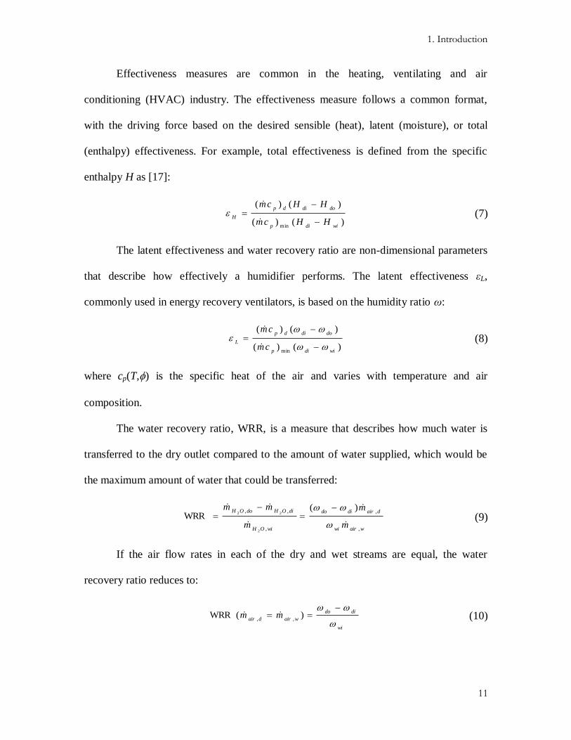
Effectiveness measures are common in the heating, ventilating and air

conditioning (HVAC) industry. The effectiveness measure follows a common format,

with the driving force based on the desired sensible (heat), latent (moisture), or total

(enthalpy) effectiveness. For example, total effectiveness is defined from the specific

enthalpy H as [17]:

)()(

)()(

min widip

dodidp

HHHcm

HHcm

(7)

The latent effectiveness and water recovery ratio are non-dimensional parameters

that describe how effectively a humidifier performs. The latent effectiveness εL,

commonly used in energy recovery ventilators, is based on the humidity ratio ω:

)()(

)()(

min widip

dodidp

Lcm

cm

(8)

where cp(T,) is the specific heat of the air and varies with temperature and air

composition.

The water recovery ratio, WRR, is a measure that describes how much water is

transferred to the dry outlet compared to the amount of water supplied, which would be

the maximum amount of water that could be transferred:

wairwi

dairdido

wiOH

diOHdoOH

m

m

m

mm

,

,

,

,, )(WRR

2

22

(9)

If the air flow rates in each of the dry and wet streams are equal, the water

recovery ratio reduces to:

wi

dido

wairdairmm

)(WRR

,, (10)

1. Introduction

12

The merits of each water transfer measure as a performance metric will be

evaluated in Section 2.2 to determine the most appropriate metric to use.

1.4. VARIABLES AND PARAMETERS AFFECTING WATER TRANSFER

The variables affecting the performance of humidifiers can be divided into

geometric variables, membrane properties, and parameters taken from the flow

conditions. The geometry is dictated primarily by the type of humidifier designed. This

study will focus on a plate-and-frame heat and humidity exchanger.

1.4.1. PLATE GEOMETRY

Table 1.1 presents an overview of the effects that changing the humidifier

geometry will have on the variables that contribute to humidifier performance, such as

heat transfer, water transfer, and pressure drop.

Table 1.1: Dependence of humidifier geometry characteristics on performance

Geometry Affects…

channel height*

heat and mass transfer coefficients, and fluid velocity through

cross sectional area

channel width*

heat and mass transfer coefficients, and fluid velocity through

cross sectional area

channel length* useable membrane area, and heat transfer coefficient through

extended surface area effectiveness

number of plates* flow rate per channel

number of channels* flow rate per channel

rib width* convective heat transfer in the form of effectiveness of extended

surface area

channel shape* heat and mass transfer coefficients; incorporated into the model

through the hydraulic diameter and assuming a rectangular aspect

ratio

* incorporated into the model

1. Introduction

13

1.4.2. MEMBRANE PROPERTIES

As described in Section 2.4.1, the focus of this research is to create a model based

on sorption-diffusion theory. This method, as opposed to the permeation method, requires

characterizing the membrane and obtaining its sorption curve. Table 1.2 lays out the

possible effects membrane properties have on humidifier performance.

Table 1.2: Dependence of membrane properties on humidifier performance

Property Affects…

membrane structure and

composition (i.e., porosity,

composite layers, etc.)*

whether transport is convective (pressure-driven) or

diffusive (concentration-driven); model assumes diffusion-

dominated transport, need sorption curves (Section 2.4.1, 0)

mechanism to be modeled:

i. membrane diffusivity* diffusive mass transfer resistance, using Fick’s First Law;

incorporated into the model (Section 0)

ii. membrane permeability convective mass transfer resistance, using Darcy’s Law;

assumed to be negligible compared to diffusion driving

force for the modes under consideration in the model

membrane conductivity* conductive heat transfer across membrane

membrane thickness* conductive heat transfer and diffusive mass transfer

resistance

* incorporated into the model

1.4.3. FLOW CONDITIONS

The flow conditions of the reactant streams are the third class of variables that

influence performance. The flow conditions are set by the wet stream supplied by the fuel

cell, and the dry stream to be humidified supplied by a blower or compressor. The effects

of these streams’ flow conditions are summarized in Table 1.3.

Table 1.3: Dependence of stream flow conditions on humidifier performance

Condition Affects…

temperature

(fluid/membrane state)

or temperature difference

(across membrane, to the

surroundings)*

relative humidity, thermo-diffusion, heat transfer and heat

loss to surroundings, and condensation rate. Also affects

membrane and fluid properties. Temperature dependence is

incorporated into the model. Temperature effects on heat loss

and condensation rate are not incorporated, yet to be

investigated

(continued on next page)

1. Introduction

14

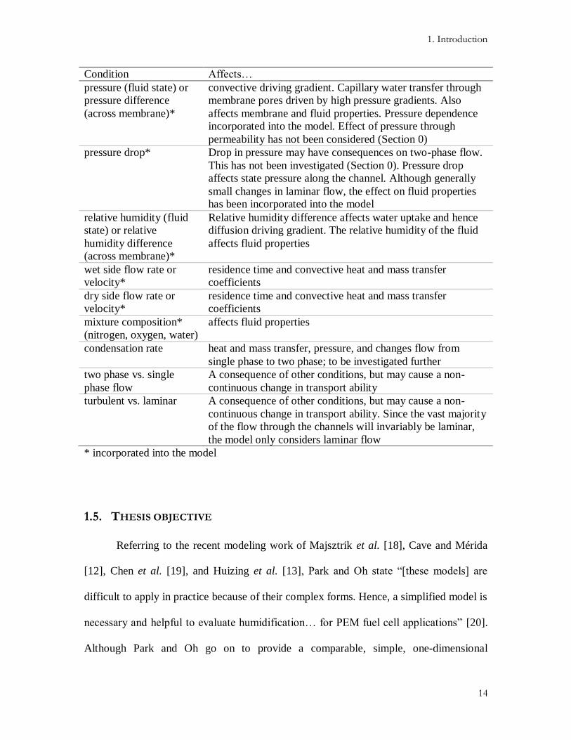
Condition Affects…

pressure (fluid state) or

pressure difference

(across membrane)*

convective driving gradient. Capillary water transfer through

membrane pores driven by high pressure gradients. Also

affects membrane and fluid properties. Pressure dependence

incorporated into the model. Effect of pressure through

permeability has not been considered (Section 0)

pressure drop* Drop in pressure may have consequences on two-phase flow.

This has not been investigated (Section 0). Pressure drop

affects state pressure along the channel. Although generally

small changes in laminar flow, the effect on fluid properties

has been incorporated into the model

relative humidity (fluid

state) or relative

humidity difference

(across membrane)*

Relative humidity difference affects water uptake and hence

diffusion driving gradient. The relative humidity of the fluid

affects fluid properties

wet side flow rate or

velocity*

residence time and convective heat and mass transfer

coefficients

dry side flow rate or

velocity*

residence time and convective heat and mass transfer

coefficients

mixture composition*

(nitrogen, oxygen, water)

affects fluid properties

condensation rate heat and mass transfer, pressure, and changes flow from

single phase to two phase; to be investigated further

two phase vs. single

phase flow

A consequence of other conditions, but may cause a non-

continuous change in transport ability

turbulent vs. laminar A consequence of other conditions, but may cause a non-

continuous change in transport ability. Since the vast majority

of the flow through the channels will invariably be laminar,

the model only considers laminar flow

* incorporated into the model

1.5. THESIS OBJECTIVE

Referring to the recent modeling work of Majsztrik et al. [18], Cave and Mérida

[12], Chen et al. [19], and Huizing et al. [13], Park and Oh state ―[these models] are

difficult to apply in practice because of their complex forms. Hence, a simplified model is

necessary and helpful to evaluate humidification… for PEM fuel cell applications‖ [20].

Although Park and Oh go on to provide a comparable, simple, one-dimensional

1. Introduction

15

thermodynamic model for a liquid-to-gas Nafion membrane humidifier, they fall short of

contributing a comprehensive model that may be used in gas-to-gas membrane

humidifiers. Their model fails to take into account the convective effects of the flow, and

not just the permeability of the selected membrane based on its thickness.

Others have focused on the shell-and-tube design of Nafion membrane

humidifiers [19,21,22]. Fuel cell system integrators are seeking to phase out Nafion as a

membrane for PEMFC humidification due to its prohibitively high price (at least $500/m2

[23]), as it is also the usual membrane used in the MEA of the fuel cell stack. The work

of Monroe et al. is primarily concerned with characterization of membranes, specifically

quantifying the interfacial characteristics of Nafion using a simple experimental chamber

where the feed gas is circulated and exchanged [24]. Monroe presented a method for

obtaining a vaporization-exchange rate coefficient from water vapor permeation

experiments for use in his model.

The empirical method applied by Huizing is a simple design parameter that

compares the theoretical diffusion time for liquid water from a membrane surface to the

residence time of the water vapor in the humidifier [25]. A more detailed thermodynamic

model is sought after that will take into account the fundamental physical mechanisms

affecting water transport. In that vein, the present work builds on the previous work of

Cave [26], but is applicable to various membranes and uses a less complex method.

The effectiveness-number of transfer units (ε-NTU) method is well-known in heat

exchanger design for determining the unknown properties of outlet fluid streams, or for

setting geometrical and flow parameters to achieve the required composition at the outlets

[27,28]. Analyses of heat transfer and mass transfer of water are coupled for attaining the

1. Introduction

16

outlet conditions in an enthalpy exchanger. The formulations of Zhang and Niu of latent

effectiveness εL and number of transfer units for moisture transfer NTUL [29] were

extended for use in a membrane heat and humidity plate-and-frame exchanger for use

with PEMFC applications. Zhang and Niu, basing their work on the previous work of

Simonson and Besant, demonstrated the dependence of performance on membrane type,

characterized by its sorption curve (water uptake vs. relative humidity) [29,30].

Table 1.4 lists the related research that is available in the literature, and specifies

any comments that relate to the present work. As mentioned earlier, a thermodynamic

model that is easy to apply will greatly assist in the design of PEMFC humidifiers. To

that end, it is necessary that the model can account for the elevated temperatures,

pressures, flow rates, and humidity found in PEMFC operation. It is not certain that

Nafion will be the membrane commonly used in commercial fuel cell humidifiers;

therefore the model should allow for other membrane types, and not be limited in scope

to one architecture, such as shell-and-tube. The column named ―Overall approach‖ in

Table 1.4 refers to a model that takes a more general approach to modeling, compared to

the complex methods requiring discretizing the flow regime.

In the present work a more comprehensive set of conditions, such as elevated

temperatures indicative of fuel cell operation, were evaluated for the mathematical model

used in HVAC energy recovery ventilator (ERV) systems. Some of the simplifications

and assumptions made during the mathematical derivation by Zhang and Niu are

analyzed for the situation in PEMFC membrane heat and humidity exchangers. The

results of an alternative approach were compared with results using the method proposed

by Zhang and Niu. Moreover, experiments were conducted with two different types of

1. Introduction

17

membrane, and correlations were found demonstrating that the proposed model can

accommodate the data and predict water transfer in membrane humidifiers.

Table 1.4: Summary table comparing relevant past research from Zhang and Niu [29,31,32], Huizing [25],

Cave [26], Chen and Peng [19,22], Monroe and Romero [24], Park, Choe, Choi [21], and Park and Oh

[20,33]

Fuel cel

l con

dition

s

Multi

ple m

embra

nes

Gen

eral

arc

hitect

ure

Ove

rall

appro

ach

Mod

el

Exp

erim

enta

l

Comments

Zhang and Niu

(1999-2002)× × × × ×

Expanded the effectiveness-NTU method of heat exchangers

for latent transfer; atmospheric conditions only; experiments

conducted with cross flow energy recovery ventilators

Huizing (2007) × × × ×

Reported on a simple empirical method to aid in design of

planar PEMFC membrane humidifiers; reported on a variety

of membranes for possible use in PEMFC humidifiers

Cave (2007) × × ×

Developed a discretized thermodynamic model based on

Nafion planar PEMFC humdifiers; applied part of the latent

effectiveness method to discretized model

Chen and Peng

(2005, 2008)× × × ×

Developed a dynamic and static thermodynamic model for a

Nafion tube-and-shell PEMFC humidifier; validated model

using a Perma Pure humidifier with fitted diffusion coefficient

Monroe and

Romero (2008)× × ×

A complex analytical model was developed for planar Nafion

membranes for determining interfacial kinetics, and was

correlated with experimental data from simple chamber tests

Park, Choe, Choi

(2008)× × ×

A dynamic and static thermodynamic model was created

based on a Nafion shell-and-tube humidifier, and validated for

different flow rates only; different geometric factors were

experimentally studied using Perma Pure humidifiers

Park and Oh

(2005, 2008)× × × ×

Provided a 1D analytical model using permeability, applied to

planar Nafion PEMFC humidifiers; liquid-to-gas only, with

some redundant results

Kadylak (2009) × × × × × ×

Extension of latent effectiveness to PEMFC gas-to-gas

membrane humidifiers, with a divergence from Nafion and

analysis of 2 different types of membrane; the thermodynamic

model is validated with experiments

In summary, the contributions to the knowledge field presented in this thesis are:

Evaluation of performance metrics, identifying the most appropriate for fuel cell

membrane humidifiers;

1. Introduction

18

Characterization of the sorption isotherms, water transfer performance, and

diffusivity of two different types of membranes;

A simple humidifier model, yet comprehensive enough for use with PEM fuel cell

applications; and,

Validation of the heat and mass transfer model with experimental data.

1.6. THESIS OVERVIEW

Figure 1.4 lays out the overview of this thesis. The introduction is presented first

which ends in the previous section with a literature review of recent relevant

investigations pertaining to membrane humidification. The next chapter outlines the

experimental setup as a precursor to all the experiments that follow in the research

presented. A study evaluating the different performance measures and a study on the

parameters affecting water transfer are given within that chapter. Another subsection in

Chapter 2 is about membrane characterization, which is required before getting into the

heat and mass transfer model. The second chapter ends with the results of the

independent experiments conducted on the two different membranes. With the

background provided, Chapter 3 goes into the simple thermodynamic model based on

heat exchanger design methodology, which is at the core of the thesis. The validation of

the model with the experimental data obtained and presented in Chapter 2 concludes the

chapter on the thermodynamic model. Finally, conclusions and thoughts on further work

are presented in the last chapter.

1. Introduction

19

Figure 1.4: Overview structure of thesis

1. Introduction and

Literature Review

2. Experimental

Performance Measure

Evaluation

Parameter Study

3. Thermodynamic

Model 4. Conclusions

Model Validation

Membrane

Characterization

20

2. EXPERIMENTS

2.1. EXPERIMENTAL SETUP

2.1.1. TEST STATION

An Arbin 50 W Fuel Cell Test Station (FCTS) which was used to conduct the

model validation and membrane experiments is schematically shown in Figure 2.1. Dry

compressed air from the laboratory is supplied to the back of the test station. A tee in the

tubing was introduced to supply what would later become the wet and dry streams. For

the dry stream, the air passes through a mass flow controller to regulate the flow rate. The

dry air is then heated to the desired temperature, before entering the dry inlet port of the

humidifier, which has been submerged in an isothermal water bath kept at a constant

temperature, Tiso. For the wet stream, the compressed air first passes through a mass flow

meter, then through a water gas bubbler, set at Tdp,wi, where the stream’s temperature will

also be raised close to Tdp = Tdp,wi. It will then be heated to the preset Twi temperature,

which is generally set at a higher temperature than the dew point temperature Tdp,wi to

prevent condensation, before entering the wet inlet port of the humidifier. Both streams

are exhausted to atmosphere to prevent any backpressure, as indicated in Section 0. At

the dry outlet the humidity sensor is placed in line with the stream to capture the wet

outlet temperature and humidity. The humidity sensor used is the HMT337 series of the

Vaisala Humidicap humidity and temperature transmitter. The sensor has a relative

humidity accuracy of 1.5% + 1.5% of the reading over a range of –40°C to 180°C. This

translates into a dew point temperature accuracy of 1°C or better in the range of test

temperatures and at a relative humidity of at least 56% [34]. This polymer-based

2. Experiments

21

capacitive humidity sensor is also placed in contact with the water in the water bath to

maintain the same temperature.

mass flow

controller

water bubbler

heater

Twi

heater

Tdi

di do

wiwo

comp. air

mas

s fl

ow

contr

oll

er

humidity

sensor

plate and frame

membrane humidifier

isothermal water bath at Tiso

Qair,d

Qair,w

Tdp,wi

wi = 1

Pwo = 0

Pdo = 0

Tdo

do

di0

Figure 2.1: Experimental setup of test station in line with test humidifier

Preliminary testing on the effects of pressure and temperature parameters, along

with the performance metric evaluations, was performed on a Greenlight Power 5 kW

G6820 test station with a plate-and-frame membrane prototype humidifier. The test setup

follows much the same as outlined in Figure 2.1 without the isothermal water bath. An

exception is the use of a contact spray humidifier instead of the gas bubbler to attain the

desired dew point temperature of the wet stream. Another difference was the use of

gravimetric water balance measurements instead of using a humidity sensor to obtain the

amount of water transferred over a period of time, typically 10 min.

2.1.2. HUMIDIFIER

The humidifier used in the membrane and validation experiments was a single

layer plate-and-frame single cell as shown in Figure 2.2. It is made from two plates of 1

in thick acrylic, with seven channels in parallel machined 1 mm deep. The channels are 3

2. Experiments

22

mm wide and are separated by 1.5 mm lands. The flow enters and exits each side through

push-connect elbow adaptors and then spreads out to the seven channels. The membrane

sample to be tested is placed in between each plate, with a 0.05 mm PTFE film creating a

seal on either side of the membrane and acrylic plate. The entrance and exit areas of the

membrane are covered with a thin sheet of water and air-impermeable polyimide film so

that only the channel areas are exposed to the flow, eliminating any entrance and exit

effects on water transfer and allowing the flow to become fully developed. The channel

length exposed for water transport is 135 mm. Four ports have been made available to

allow thermocouples to be placed into the flow and measure the temperature of each

stream. A Type T thermocouple was placed through a hole drilled in a plastic pipe fitting

plug.

Figure 2.2: Experimental single cell humidifier with installed ports

TTwwii

Qwo

Qwi Qdo

Qdi

2. Experiments

23

A full subscale prototype humidifier was used for the initial performance metric

and parameter study tests. The humidifier was a dPoint Technologies Px3-46mm

consisting of 40 plates of 16 channels each, with a perfluorinated composite ionic

membrane. The housing of the humidifier was made from polyester to provide rigid

support and keep the humidifier insulated.

2.1.3. MAINTAINING ISOTHERMAL CONDITIONS

Isothermal conditions were necessary to prevent any condensation from occurring

within the test module, as this would introduce another factor which is a challenge to

model. Constant-temperature conditions allow for a controlled environment in which the

water transfer can be isolated from any heat transfer that may occur in a humidifier, and

focuses the study on the water transport across the membrane being tested. To this end,

the humidifier was submerged in water contained in a Cole-Parmer BT-15 heated

circulating water bath, along with the hollow adaptor which housed the humidity sensor.

The connections were made as close as possible to the water level, hence the upright

orientation as shown in Figure 2.2. The water bath was kept at 1°C higher than the wet

side dew point to prevent condensation when the test station feedback control overshot

the dew point temperature set point. The inlet gas temperatures were also set higher than

the dew point so as to prevent condensation, and the thermocouples placed in the

humidifier at the inlet or outlet of each stream provided feedback for the test station gas

temperature set point.

2.2. EVALUATION OF PERFORMANCE MEASURES

Experiments were conducted to determine how the humidifier performance varied

with changes in operating temperature or in pressure differential across the membrane.

2. Experiments

24

The first experiment was to run the humidifier with the wet and dry inlet streams

set with equal temperatures, ranging from 65°C to 80°C, at 100 SLPM and no

backpressures. The performance of the humidifier is plotted in terms of the dew point

approach temperature, water transfer rate, and water recovery ratio in Figure 2.3. The

DPAT compensates for using dew point temperature alone in that the performance

decreases in terms of DPAT as temperature increases, yet the actual dry outlet dew point

temperature increases. Only using the dry outlet dew point temperature would be

misleading, as an increase in dew point does not necessarily mean better performance. On

the other hand, the water transfer rate is increasing as the temperature increases, but this

can be explained by the fact that there is more water mass available to be transferred for

the higher saturated wet inlet temperatures. The water recovery ratio accounts for the

extra water that is available as the temperature increases, and shows that the humidifier

performance decreases in relative terms as the inlet temperatures increase.

Px3-P-19-046mm-40PL-AC - 0.85-0.85 IM IM; Membrane D

di = 0%, P do = 0 kPag, Q air,d = 100 SLPM

wi = 100%, P wo = 0 kPag, Q air,w = 100 SLPM

0

5

10

15

20

25

30

60 65 70 75 80 85

Temperature T di = T wi (ºC)

DP

AT

(ºC

)

0

0.1

0.2

0.3

0.4

0.5

0.6

0.7

0.8

0.9

1

Wat

er T

ransf

er (

g/s

) | W

RR

Dew Point Approach Temperature (ºC)

Water Transfer Rate (g/s)

Water Recovery Ratio

Figure 2.3: Water transfer as operating temperature is changed

2. Experiments

25

In the second experiment, the dry inlet stream was kept at 25°C and the wet inlet

stream was supplied saturated at 65°C, both streams with an air flow rate of 100 SLPM.

This time the dry outlet backpressure was increased from ambient to 35 kPag, while

keeping the wet outlet backpressure at atmospheric pressure, creating a pressure

differential across the membrane of up to 35 kPa. This is equivalent to a pressure ratio of

up to 1.35 (136 kPaa/101 kPaa). The dew point approach temperature, water transfer rate,

and water recovery ratio are once again plotted, this time in Figure 2.4. In the previous

experiment, the slopes of the DPAT and WRR diverged, while in this experiment the

slopes are both negative. In this case, the DPAT signifies that the humidifier is

performing better as the pressure differential increases, yet both the water transfer rate

and WRR suggest that the humidifier is actually performing worse as the pressure

differential increases. In conclusion, the dew point temperature or dew point approach

temperature is a misleading measure of humidifier performance, and should be avoided.

In both experiments, the same amount of membrane area was used, so the water flux

would give the same results as the water transfer rate. The absolute measure of water

transfer rate does not adequately account for the change in available water at different

flow conditions for the same humidifier; though it may be a good measure for comparing

different humidifiers at the same operating conditions. A better measure is the water

recovery ratio, which takes into account the amount of water supplied as the operating

conditions change; however, it is difficult to determine if an adequate amount of water is

supplied to the fuel cell with the water recovery ratio alone, so the necessary WRR would

need to be calculated beforehand based on the operating conditions. Therefore, because

the required operating conditions of the fuel cell will change with loading, it is proposed

2. Experiments

26

that water recovery ratio be used as the preferred performance metric, as it will take into

account the different amount of water supplied at each flow rate and flow conditions.

Px3-P-19-046mm-40PL-AC - 0.85-0.85 IM IM; Membrane D

T di = 25ºC, di = 2%, Q air,d = 100 SLPM

T wi = 65ºC, wi = 100%, P wo = 0 kPag, Q air,w = 100 SLPM

0

2

4

6

8

10

12

14

16

0 5 10 15 20 25 30 35 40

Dry Out Pressure P do (kPag)

DP

AT

(ºC

)

0

0.1

0.2

0.3

0.4

0.5

0.6

0.7

0.8

0.9

1

Wat

er T

ransf

er (

g/s

) | W

RR

Dew Point Approach Temperature (ºC)

Water Transfer Rate (g/s)

Water Recovery Ratio

Figure 2.4: Water transfer as dry stream pressure is changed

2.3. PARAMETER EFFECT STUDY

As can be seen from Section 1.4, there are many variables that could be studied,

resulting in a very large experimental matrix. To determine if the potential experimental

matrix could be condensed by eliminating a possible variable, such as temperature or

pressure, the plate-and-frame membrane prototype humidifier described in Section 2.2

was tested on the same Greenlight Power 5 kW G6820 test station.

The first test conducted was to increase the dry incoming air temperature in

increments of 5°C until it met the wet inlet temperature, maintained at 80°C, with

ambient backpressures on both streams. The range of temperature was chosen such that it

represented the typical range found in operating fuel cell temperatures, with the minimum

2. Experiments

27

temperature taken to be close to room temperature, or 25°C. These dry inlet temperatures

were normalized over the range of operating conditions to facilitate comparison with

pressures in the subsequent experiments. The testing conditions are outlined in Table 2.1,

and the results of the temperature dependence test are displayed in Figure 2.5. Linear

regression analysis of the dry outlet dew point against normalized temperature data

demonstrates a slope of –8.17°C (R2 = 0.935).

Table 2.1: Experimental matrix for temperature-dependence testing

Membrane Control Flow Rate Temperature (Tdi) Dependent

Membrane D: perfluorinated

ionic composite

Twi = Tdp,wi = 80°C Tdp,di = –20°C

Pdo = Pwo = 0 (gauge)

100 SLPM 25°C … 80°C WRR

Tdo

Tdp,do

Px3-P-19-046mm-40PL-AC - 0.85-0.85 IM IM; Membrane D

di = 2%, P do = 0 kPag, Q air,d = 100 SLPM

T wi = T max = 80ºC, wi = 100%, P wo = 0 kPag, Q air,w = 100 SLPM

T dp,do = –8.1731x + 66.545

R2 = 0.9348

30

35

40

45

50

55

60

65

70

75

80

0 0.2 0.4 0.6 0.8 1

Normalized Dry In Temperature (T di – T min)/(T max – T min)

Td

o T

emp

erat

ure

(ºC

)

0

0.1

0.2

0.3

0.4

0.5

0.6

0.7

0.8

0.9

1

WR

R (ω

do

– ω

di)/ω

wi

Dry-Bulb Temperature (ºC)

Dew Point Temperature (ºC)

Water Recovery Ratio

Figure 2.5: Effect on water transfer of changing dry inlet temperature

The next test performed was to maintain constant inlet temperature while

changing the dry air outlet backpressure from ambient to 35 kPa gauge. The range of

2. Experiments

28

pressure observed across the membrane is dictated by the pressure drop across a fuel cell

stack, which is normally below 5 psi (35 kPa). These dry outlet pressures were

normalized and the results of this test are shown in Figure 2.6. Linear regression (R2 =

0.97) through the dry outlet dew point temperature points in this graph gives a slope of

2.58°C. Table 2.2 outlines the testing conditions of both pressure dependence tests.

Table 2.2: Experimental matrix for pressure-dependence testing

Pressure (kPag)

Membrane Control Pwo Pdo,min Pdo,max Dependent

Membrane D: perfluorinated

ionic composite

Twi = Tdp,wi = 65°C Tdi = 25°C; Tdp,di = –20°C

Qair,d = Qair,w = 100 SLPM

0 0 35 WRR

Tdo

Tdp,do

Membrane D:

perfluorinated

ionic composite

Twi = Tdp,wi = 65°C

Tdi = 25°C; Tdp,di = –20°C

Qair,d = Qair,w = 100 SLPM

120 120 155

WRR

Tdo

Tdp,do

Px3-P-19-046mm-40PL-AC - 0.85-0.85 IM IM; Membrane D

T di = 25ºC, di = 2%, Q air,d = 100 SLPM

T wi = 65ºC, wi = 100%, P wo = P min = 0 kPag, Q air,w = 100 SLPM

T dp,do = 2.5823x + 53.098

R2 = 0.9704

15

20

25

30

35

40

45

50

55

60

65

0 0.2 0.4 0.6 0.8 1

Normalized Dry Out Pressure (P do – P min)/(P max – P min)

Td

o T

emper

ature

(ºC

)

0

0.1

0.2

0.3

0.4

0.5

0.6

0.7

0.8

0.9

1

WR

R (ω

do

– ω

di)/ω

wi

Dry-Bulb Temperature (ºC)

Dew Point Temperature (ºC)

Water Recovery Ratio

Figure 2.6: Effect on water transfer of changing dry out backpressure, low total pressure

2. Experiments

29

Operation at elevated pressures is required for many fuel cell systems, such as in

automotive applications, so a similar test was performed at these pressures. Even at

elevated pressures, the fuel cell stack will rarely incur pressure drops greater than 5 psi

(35 kPa). In this test the dry outlet backpressure ranged from 120 kPag to 155 kPag,

while maintaining the wet outlet backpressure at 120 kPag. The outcome is displayed in

Figure 2.7. The dry side outlet pressures were likewise normalized in the plot.

Px3-P-19-046mm-40PL-AC - 0.85-0.85 IM IM; Membrane D

T di = 25ºC, di = 2%, Q air,d = 100 SLPM

T wi = 65ºC, wi = 100%, P wo = P min = 120 kPag, Q air,w = 100 SLPM

15

20

25

30

35

40

45

50

55

60

65

0 0.2 0.4 0.6 0.8 1

Normalized Dry Out Pressure (P do – P min)/(P max – P min)

Td

o T

emper

ature

(ºC

)

0

0.1

0.2

0.3

0.4

0.5

0.6

0.7

0.8

0.9

1

WR

R (ω

do

– ω

di)/ω

wi

Dry-Bulb Temperature (ºC)

Dew Point Temperature (ºC)

Water Recovery Ratio

Figure 2.7: Effect on water transfer of changing dry out backpressure, high total pressure

At the high total pressures, the effect of changing the pressure in one gas stream

has little effect on the water transfer. Likewise, at the lower total pressures—close to

atmospheric pressure—comparing the slopes of the best fit lines reveals that the

temperature difference between the inlets of the streams plays a larger role on water

transfer than pressure difference between streams for the range of temperature differences

2. Experiments

30

and pressure differences seen in practical fuel cell operation. Therefore, since the dry side

outlet dew point temperature varies by up to a factor of three over the tested range, it was

decided that the effect of temperature would be the focus of the ongoing analysis of

membrane water transfer in plate-and-frame humidifiers, and that the effect of pressure

would be neglected by conducting all simulations and experiments at atmospheric

conditions.

2.4. MEMBRANE CHARACTERIZATION

2.4.1. SOLUTION-DIFFUSION AND SORPTION CURVES

In porous solid membranes, the main mechanisms of water transfer are surface

diffusion into the membrane and liquid flowing through the membrane by capillary

condensation. A water concentration gradient from the water molecules adsorbed on the

pore walls and diffusing on the surface is the driving force in surface diffusion [35]. The

primary mass transfer of permeating species from the wet side to the dry side can be

broken down into three steps [32]; i.e.:

1. Adsorption at the supply side of the membrane;

2. Diffusion through the membrane as described by adsorption isotherms;

3. Desorption at the sweep side of the membrane.

Solution-diffusion theory models water transport as a flux proportional to a

driving gradient. Analogous to the conduction equation in heat transfer known as

Fourier’s Law, in the case of mass diffusion the diffusion equation for flux of species A

in medium B is known as Fick’s Law, and the proportionality constant is the binary

diffusion coefficient or mass diffusivity, denoted by DAB [28]:

2. Experiments

31

AABA

DJ (11)

where Φ is a placeholder variable for the potential driving force, which may be mass

based (density), mol based (concentration), chemical potential based, etc. Depending on

the driving force chosen, the diffusivity will need to be adjusted or multiplied by a factor

to maintain the correct units.

For a membrane with a hygroscopic polymer component, water transport

increases with an increase in humidity. For these types of membranes, a sorption

isotherm (or water uptake curve) provides the response of the membrane with change in

average relative humidity. On the other hand, if the pore structure is large enough, such

as in porous textiles, water vapor will transport through the gas-filled pore structure. In

these membrane types, generally not suitable for PEMFC humidification due to air cross-

over, water vapor diffusion does not depend on relative humidity since the water vapor

simply diffuses through pore voids [36].

For membranes which exhibit small diffusion coefficients requiring long

experiment times, the sorption technique is preferred to the permeation technique [37].

The sorption technique of quantifying water uptake is performed using a dynamic

gravimetric vapor sorption (DVS) instrument. A small sample of the membrane (< 1 cm2)

is suspended on a quartz spring, which measures the weight of the membrane as it

absorbs or desorbs water with an ultra-microbalance. The membrane is kept in a chamber

where the temperature and humidity are controlled by mixing saturated and dry carrier

gas streams through mass flow controllers, and the whole instrument is kept in an

incubator to keep it isothermal [38]. The sorption isotherms of two different membranes,

which will be later used in the study, are described in the next two sections.

2. Experiments

32

2.4.2. WATER UPTAKE OF A HYDROPHILIC-IMPREGNATED POLYMER

Much testing and data have been collected on DuPont NafionTM

membranes in

industry and in the literature. However, due to their exorbitant cost they are not expected

to be used in future humidifier systems, hence the need to acquire more commercially

feasible membranes as outlined in the Introduction. Furthermore, there are disparate data

on Nafion’s sorption and diffusivity values in the literature, as reported by Cave [26],

making it difficult to use for practical modeling. With this in mind, it was decided to

concentrate on a commercially available membrane. The chosen porous-type membrane

is made from a hydrophilic-filled polymer. It has a porosity of approximately 70%,

thickness of 0.15 mm, and hydrophilic additive to polymer ratio of 2.5. It further contains

15% plasticizer mineral oil used in the extrusion process. Due to its commercial

availability, this membrane (labeled Membrane E), is very low in cost, in the range of

$3/m2. The membrane is coated in a 4% Nafion (PFSA) DE2021 dispersion to decrease

the air crossover, and baked at 100°C for 1 h to help anneal the Nafion.

Three samples of the porous polymer with hydrophilic additive membrane were

characterized using a Surface Measurement Systems (UK) vapor sorption instrument as

described in the previous section. The samples’ sorption and desorption curves were

characterized at 25°C, as past attempts to perform experiments at high temperatures on

the DVS equipment have failed. Each sample was first dried to < 1% relative humidity to

determine its dry mass. The relative humidity was then increased stepwise in 10%

increments up to 90%, then to 94% and 97%. The relative humidity was then decreased

following the same profile to obtain the desorption curve. Mass equilibrium was obtained

at each step before moving on to the next humidity setting. Mass equilibrium was reached

when the change in mass with respect to total mass of the sample was less than 0.1%, or

2. Experiments

33

dm/dt < 0.001. The sorption and desorption profiles were discovered to be nearly equal.

All six profiles (three absorption and three desorption) of the porous polymer-hydrophilic

additive membrane with PFSA coating were averaged and are plotted with their 95%

confidence interval error bars in Figure 2.8. A third-degree polynomial was used to curve

fit the data up to 80% relative humidity, with an R2 value of 0.996. The curve past 80%

relative humidity is then fitted to a general isotherm curve for water uptake θ:

CC

1

max (12)

where the maximum moisture content is θmax = 2.5, and the value of constant C = 148.

With a value of C in the order of 100, indicating a low uptake for most of the low end of

relative humidity and a sharp slope at the very high end of relative humidity, this porous

membrane is characterized as Type III Extreme (Type IIIE) [39]. Several desiccant

polymers exhibit Type III behavior, with a great increase in uptake only at values greater

than 90% relative humidity [32].

θ = 3E−73 – 4E−5

2 + 0.0018 + 0.0014

R2 = 0.9959

0

0.5

1

1.5

2

2.5

0 10 20 30 40 50 60 70 80 90 100

Relative Humidity (%)

Wat

er U

pta

ke

θ (

kg w

ater

/kg m

embra

ne)

θ = 2.5/(1 – 148 + 148/ )

> 80%

Figure 2.8: Sorption isotherm at 25°C of hydrophilic additive-impregnated porous polymer membrane

2. Experiments

34

Due to limitations encountered in the past with using the dynamic vapor sorption

instrument, an isotherm was only obtained at 25°C; however, up to moderate

temperatures the sorption curve tends to be independent of temperature [40].

2.4.3. WATER UPTAKE OF A PERFLUORINATED COMPOSITE MEMBRANE

One of the disadvantages of the porous polymer membrane is its limited lifetime

in fuel cell operation. It has been hypothesized that the physical adhesion between

hydrophilic additive and polymer degrades under wear, leading to the loss of hygroscopic

additive from the polymer matrix [25]. A new membrane has been obtained which has

logged over 5000 h at fuel cell operating conditions without degradation compared to the

approximately 3000 h lifetime experienced by the incumbent, baseline porous polymer

membrane described in the previous section. The new membrane is an ionic composite,

with a middle layer of perfluorinated composition, and hydrophobic outer layers. As

described earlier, an ionic membrane has a water transport mechanism similar to that of

Nafion, where clusters of water are transported across the thickness of the membrane due

to the ionic bases. The overall thickness of this membrane is 0.02 mm. This membrane is

proprietary technology, so its description must be kept confidential.

The vapor sorption experiment was repeated with samples of the ionic

perfluorinated composite membrane. The experimental temperature (25°C) and relative

humidity profile was kept the same as with the polymer-hydrophilic additive membrane.

The sorption isotherm is displayed in Figure 2.9. With a maximum water uptake of θmax =

0.217, and the value of C = 9.23, this membrane also exhibits Type III behavior, only

experiencing increased water uptake at high relative humidities. A third-degree

2. Experiments

35

polynomial fit (R2 = 0.999) was also obtained for relative humidities less than 80% to be

integrated into the model.

θ = 2E−73 – 2E−5

2 + 0.0013 + 0.0022

R2 = 0.9995

0

0.05

0.1

0.15

0.2

0.25

0 10 20 30 40 50 60 70 80 90 100

Relative Humidity (%)

Wat

er U

pta

ke

θ (

kg

wat

er/k

g m

emb

ran

e)

θ = 0.217/(1 – 9.23 + 9.23/ )

> 80%

Figure 2.9: Sorption isotherm at 25°C of ionic perfluorinated composite membrane

2.4.4. COMPARISON OF THE POROUS AND IONIC MEMBRANES

The sorption isotherms of the polymer-hydrophilic additive, PFSA coated and

perfluorinated composite membranes were plotted on the same graph in Figure 2.10. The

two membranes show the same water uptake characteristics up to 80% relative humidity.

However, the porous polymer membrane exhibits a much higher maximum water uptake

compared to the ionic perfluorinated composite membrane. At 97% relative humidity, the

porous membrane is able to absorb 2.6 times as much water as the ionic membrane on a

membrane mass basis, which already takes into account the thickness of each membrane.

One hypothesis, in accordance with observation, is that the porous polymer membrane,

being hydrophilic, absorbs liquid water into the structure of the membrane. Whereas the

ionic membrane, with its hydrophobic outer layers, prevents liquid water from wetting on

2. Experiments

36

the surface and therefore inhibits water absorption, or due to the fact that a high weight

percentage of the membrane is the hydrophobic layers, which does not sorb water vapor.

0

0.05

0.1

0.15

0.2

0.25

0.3

0.35

0.4

0.45

0.5

0 10 20 30 40 50 60 70 80 90 100

Relative Humidity (%)

Wat

er U

pta

ke

θ (

g w

ater

/g m

embra

ne)

hydrophilic porous polymer

ionic perfluorinated composite

Figure 2.10: Comparison of sorption isotherm at 25°C of a porous and an ionic membrane

2.5. EXPERIMENTAL DESIGN

The mathematical model developed in Chapter 3 requires some fitted parameters,

such as the diffusivity of water in the membrane, in order to be adequately used over a

range of temperatures. This chapter lays out the experiments undertaken to validate the

model, to gain confidence in its results and to obtain the values for parameters described

in Section 3.7 that are required for its practical use. Once the model has been verified, it

will then be ready to be used for different conditions or different geometries, more in

accord with the scale of commercial products. The dependent variable to be obtained will

be the water transfer as taken from measurements of water at the outlet of the dry stream.

2. Experiments

37

2.5.1. TEST MATRIX AND CONDITIONS

A difference in fuel cell humidification as compared to ERV systems is that the

wet stream entering the humidifier is generally saturated. Heat transfer occurs when there

is a difference in temperature. Thus, water condensation, and hence two-phase flow, is

inevitable in the wet flow of fuel cell membrane humidifiers if there is any temperature

difference between the flows or the surroundings. Therefore isothermal conditions are

chosen to perform comparison of humidifier performance at different flow rates, and the

effects of condensation and two-phase flow are suggested as topics for further

investigation.

Since the sorption curves were obtained at 25°C, one set of experiments were

conducted at a benchmark temperature of 25°C, even though fuel cell systems will for the

majority of their time operate at higher temperatures. As discussed in Section 3.4.1, an

average fuel cell operating temperature of 50°C is more appropriate for backup and

portable applications. This gives another temperature at which to conduct experiments.

There is also a trend to operate fuel cells at higher temperatures, as in forklift and

automotive applications. From a survey of customer specifications available to dPoint

Technologies for applications at higher temperatures, another operating temperature was

chosen at 75°C. Therefore, the experiments to be conducted are three equally spaced

isothermal temperatures: 25°C, 50°C and 75°C.

It is necessary to test a range of flow rates; both because the humidifier will see

different demands as the fuel cell operates through a range of power, and because it is

required in determining the rated flow of a certain humidifier design. Due to the large

number of plates to divide the flow, a plate-and-frame humidifier will always run at

laminar flow, even though design elements may be introduced to cause flow separation

2. Experiments

38

and therefore enhance heat and mass transfer. A particular plate-and-frame humidifier

designed at dPoint for backup power applications may see a Reynolds number of 80. The

proposed test jig for the humidifier experiments has 7 channels with 1 mm height and 3

mm width, with one layer for each stream. The hydraulic diameter, Dh, is found from:

mm 5.1)(2

4

dw

wdD

h (13)

The Reynolds number is defined as

wd

QDh

Re (14)

Rearranged to find the flow rate per channel, Q, using the 75°C isothermal case to

obtain the dynamic viscosity of air μ = 2.07 × 10–5

kg m–1

s–1

, and its density at STP ρ =

1.29 kg m–3

:

SLPM 154.0Re

hD

wdQ

(15)

The flow rate per stream is found by multiplying by the number of channels, n = 7, so

that the flow rate for each side is 1.08 SLPM. An Arbin 50 W Fuel Cell Test Station

(FCTS), which has mass flow controllers rated up to 1.1 SLPM and 2 SLPM for two

separate streams, was used to supply metered dry air and saturated wet air. With the

limitation of 1.1 SLPM of one stream in mind, the flow rates to be tested are at 0.4, 0.7,

and 1 SLPM.

The dry stream of the humidifier will be at a lower flow than the wet stream

because the air component coming out of the fuel cell stack will have depleted oxygen

content, having reacted with hydrogen to form water; however, the ratio of air flows on

the dry side compared to the wet side varies according to the stoichiometry used to

2. Experiments

39

supply the fuel cell with extra oxygen to react with. The higher the air stoichiometry

supplied, the closer the air flow rate on the dry side will be to the air flow on the wet side.

For this reason, a simplification is applied where the dry side and wet side air flows are

maintained equal. Water is added to the wet side air flow from a gas bubbler to saturate

the air at the given test temperature, and this water flow rate is not included in the test

conditions as wet air does not pass through the mass flow controller. The dry air is

supplied from a compressed air line, which has been measured to have a relative

humidity between 0.16% and 2.9% through the whole test temperature range (or always

lower than a –20°C dew point temperature).

As outlined in Section 0, the focus of the study is on temperature effects over

pressure effects on water transport in practical operation, so the outlets are kept at

ambient pressure. Since the chosen performance measure to be tested is the water transfer

from the wet side to the dry side, water recovery ratio (WRR) is the dependent variable to

be sought in the tests. The amount of water at the dry outlet will also be presented by the

dew point Tdp,do as a measure of the amount of water available to the fuel cell, which is

one of the parameters of water outputted by the humidity sensor. All the foregoing

variables and testing conditions as inputs and the output are laid out in the test matrix of

Table 2.3.

Table 2.3: Experimental testing matrix

Membrane Control Flow Rate Temperature (Tiso) Dependent

Membrane E:

porous polymer,

PFSA coated

Tdi = Twi = Tdp,wi = Tiso

Tdp,di = –20°C

Pdo = Pwo = 0 (gauge)

0.4 SLPM

0.7 SLPM

1 SLPM

25°C

25°C

25°C

50°C

50°C

50°C

75°C

75°C

75°C

WRR (Tdp,do)

Membrane D:

perfluorinated ionic composite

As above

0.4 SLPM

0.7 SLPM 1 SLPM

25°C

25°C 25°C

50°C

50°C 50°C

75°C

75°C 75°C

WRR

(Tdp,do)

2. Experiments

40

2.6. MEMBRANE RESULTS AND DISCUSSION

Three samples of the Nafion-coated polymer membrane with hydrophilic additive

were tested at three different flow rates and at three different temperatures according to

the conditions presented in the experimental matrix, Table 2.3, for a minimum of 27 tests.

The results of the humidifier performance in terms of water transfer through the

membrane are presented in Figure 2.11 with the measured dry outlet dew point

temperature from the humidity sensor, and the converted water recovery ratio also

plotted.

0

10

20

30

40

50

60

70

80

0 0.2 0.4 0.6 0.8 1 1.2

Air Flow Rate Q air (SLPM)

Dew

Po

int

Tem

per

atu

re

Td

p,d

o (

°C)

0

0.1

0.2

0.3

0.4

0.5

0.6

0.7

0.8

WR

R (ω

do

– ω

di)/ω

wi

Dew Point Temperature Water Recovery Ratio

Figure 2.11: Experimental results for porous polymer membrane E, at ♦ Tiso = 25°C, ● 50°C, ■ 75°C

As expected, the trend at all temperatures shows an inverse relation between flow

rate and water transfer: as the flow rate increases, the water transfer relative to amount of

supply water will decrease. In terms of water recovery ratio, the effect of decreasing

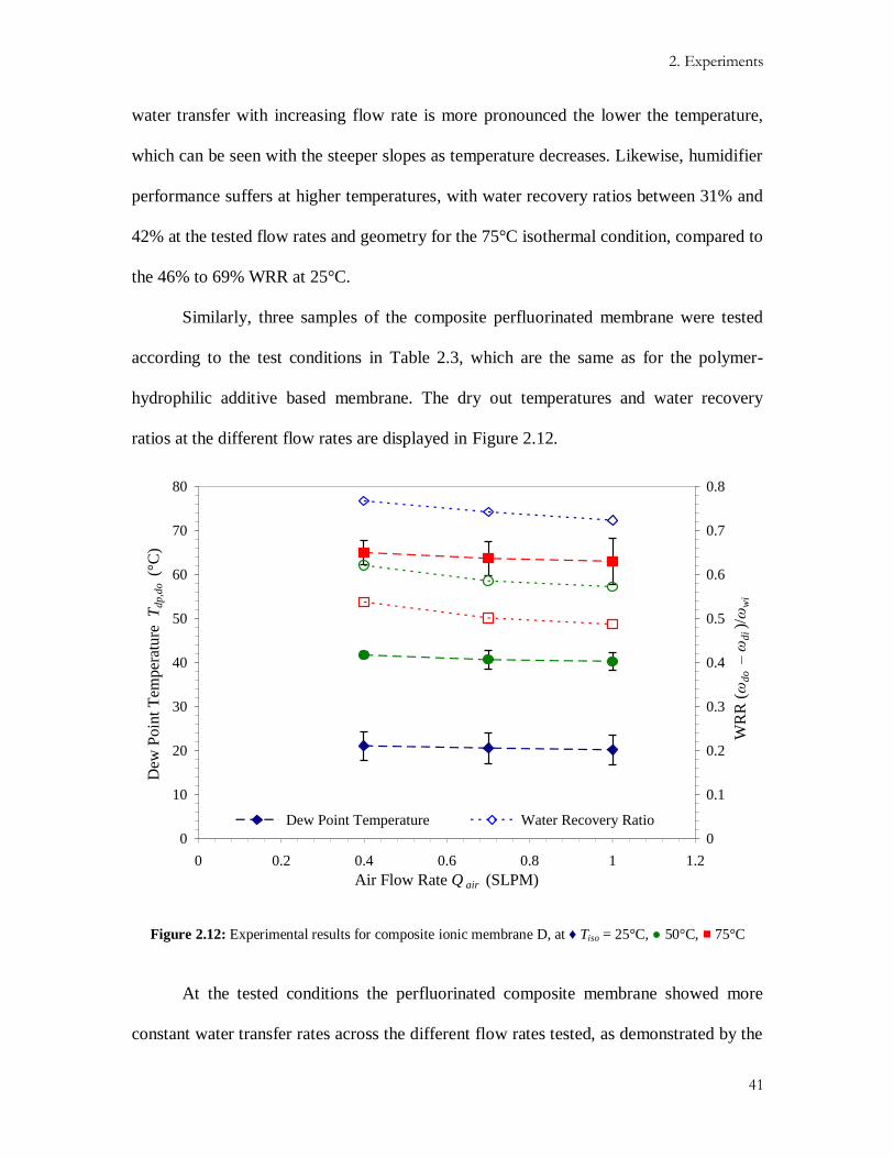
2. Experiments

41

water transfer with increasing flow rate is more pronounced the lower the temperature,

which can be seen with the steeper slopes as temperature decreases. Likewise, humidifier

performance suffers at higher temperatures, with water recovery ratios between 31% and

42% at the tested flow rates and geometry for the 75°C isothermal condition, compared to

the 46% to 69% WRR at 25°C.

Similarly, three samples of the composite perfluorinated membrane were tested

according to the test conditions in Table 2.3, which are the same as for the polymer-

hydrophilic additive based membrane. The dry out temperatures and water recovery

ratios at the different flow rates are displayed in Figure 2.12.

0

10

20

30

40

50

60

70

80

0 0.2 0.4 0.6 0.8 1 1.2

Air Flow Rate Q air (SLPM)

Dew

Po

int

Tem

per

atu

re

Td

p,d

o (

°C)

0

0.1

0.2

0.3

0.4

0.5

0.6

0.7

0.8

WR

R (ω

do

– ω

di)/ω

wi

Dew Point Temperature Water Recovery Ratio

Figure 2.12: Experimental results for composite ionic membrane D, at ♦ Tiso = 25°C, ● 50°C, ■ 75°C

At the tested conditions the perfluorinated composite membrane showed more

constant water transfer rates across the different flow rates tested, as demonstrated by the

2. Experiments

42

nearly flat curves. It is possible this may be attributed to different transfer mechanisms in

the membranes. The porous polymer membrane is porous and water absorbs into the

membrane enhanced by the hydrophilic Nafion coating, whereas in the ionic composite

membrane water is transferred according to the Grotthus mechanism of water-cluster

hopping [41,42]; also, the outer layers are hydrophobic preventing wetting and overall

absorption into the membrane. Figure 2.13 plots the water recovery ratio of the two

membranes. The perfluorinated composite membrane shows greater water transfer at all

temperatures and flow rates, from as low as 11% better at 25°C and 0.4 SLPM, and up to

56% better at 1 SLPM. One factor that makes the ionic composite membrane better for

water transfer is its thinness—it is approximately 13% as thick as the porous polymer

membrane—resulting in decreased diffusivity resistance across the membrane.

0

0.1

0.2

0.3

0.4

0.5

0.6

0.7

0.8

0.9

1

0 0.2 0.4 0.6 0.8 1 1.2

Air Flow Rate Q air (SLPM)

WR

R (ω

do

– ω

di)/ω

wi

Membrane E: porous polymer, PFSA coated

Membrane D: perfluorinated ionic composite

Figure 2.13: Comparison of water recovery ratio between two membranes, at ♦ Tiso = 25°C, ● 50°C, ■ 75°C

43

3. HEAT AND WATER TRANSFER MODEL

3.1. HEAT TRANSFER USING THE EFFECTIVENESS METHOD

In heat exchanger design, given the inlet temperatures (but not the outlet

temperatures), the preferred analysis approach is the effectiveness method. This method

is used when the flow rates and heat exchanger size and type are known. The

effectiveness method can also be used in reverse to size heat exchangers—finding the

required number of thermal units (NTU), and then selecting a heat exchanger which

meets that NTU based on the outlet flow requirements.

The effectiveness method for heat exchanger design starts by obtaining the

number of transfer units, NTU, defined as:

min

)(NTU

pcm

UA

(16)

where U is the overall heat transfer coefficient and A is the heat transfer area, which are

parameters of the heat exchanger design. Common pipe flow heat transfer correlations

are used to determine the heat transfer coefficient h, and cp is the specific heat capacity,

which is multiplied by the mass flow rate of the fluid m . Since the ε-NTU method is an

overall approach as opposed to a discretized model, all fluid property must be determined

at the average conditions of each stream, based on the inlet and outlet conditions.

Likewise, if the temperature of the membrane is required, an average temperature is used,

calculated from all stream inlet and outlet temperatures.

The effectiveness, ε, is a ratio of the actual heat transfer rate for a heat exchanger

to the maximum possible heat transfer rate in those flow conditions

3. Heat and Water Transfer Model

44

)()(

)()(

)()(

)()(

minminmax diwip

didodp

diwip

wowiwp

TTcm

TTcm

TTcm

TTcm

q

q

(17)

where the dry stream has been taken to be the cold stream, and the wet stream the hot

stream. The nomenclature will be dealt with in terms of a drier and wetter stream in order

to later apply the equations to a humidifier with hot and cold streams. Rearranging Eqn.

(17) one can find the sought-after outlet temperature if the effectiveness is known:

dodi

p

dp

didoTT

cm

cmTT

min)(

)(

(18)

Kays and London have shown that depending on the heat exchanger type, the

effectiveness is a function of NTU and Cr = Cmin/Cmax = ( m cp)min/( m cp)max [27].

1,NTU1

NTU

1,])1(NTUexp[1

])1(NTUexp[1

r

r

rr

r

C

CCC

C

(19)

which is the effectiveness for a typical counter flow heat exchanger.

Therefore, knowing the effectiveness and the inlet temperatures in addition to the

heat exchanger geometry and configuration enables the determination of the heat transfer

rate and hence the outlet temperatures.

3.2. THE CHILTON-COLBURN ANALOGY FOR MASS TRANSFER

Zhang and Niu report in [29] and [32] their application of the Chilton-Colburn

analogy. The analogy is between heat transfer and mass transfer—derived from the j

factors for heat and mass transfer—which is stated as:

MH

jj (20)

3. Heat and Water Transfer Model

45

In Ref. [32], the correct fundamental equations to the Chilton-Colburn analogy are

given, such as the j factor for heat transfer from the Stanton and Prandtl numbers

3/2PrSt

HHj (21)

where the Stanton number for heat transfer, using the Nusselt and Reynolds numbers, is

PrRe

NuSt

H (22)

Likewise the j factor for mass transfer using the corresponding Stanton number

and Schmidt number

3/2ScSt

MMj (23)

where the Stanton number for mass transfer, utilizing the Sherwood number, is

ScRe

ShSt

M (24)

Defining the Lewis number as the ratio of thermal diffusivity to mass diffusivity

[28,43]:

Pr

ScLe

ABD

(25)

and substituting Eqn. (21) to (24) into the Chilton-Colburn analogy, Eqn. (20), gives:

3/23/2

ScScRe

ShPr

PrRe

Nu

(26)

Rearranging leads to:

3/1

3/1

LeNuPr

ScNuSh

(27)

which can then be used to find the convective mass transfer coefficient as:

3/1

Le

p

Mc

hh (28)

3. Heat and Water Transfer Model

46

Since the values for the Lewis number are usually around unity for typical ERV

conditions, if the Lewis number term is ignored in the heat and mass transfer analogy the

error is not likely to carry through to a great extent through to the rest of the other

parameters, such as the overall mass transfer coefficient UL used in Eqn. (16). The

inclusion of water vapor with air will however have a greater effect on the mass transfer

coefficient than of dry air alone, due to deviations from unity in the Lewis number,

especially at higher temperatures as shown in Figure 3.1.

0

0.2

0.4

0.6

0.8

1

0 20 40 60 80 100 120

Relative Humidity (%)

Lew

is N

um

ber

s

75°C

25°C

Le1/3

Le

Figure 3.1: Variation in Lewis number term with relative humidity at different temperatures

The wet stream of a PEMFC may normally come into the heat and humidity

exchanger at around 75°C, whereas in an ERV system the temperatures are closer to

25°C. At 75°C, the value of Le1/3

at 100% relative humidity is 10.2% lower compared to

that of a stream at 0% relative humidity. This error will then be passed on to the mass

transfer coefficient as per Eqn. (28).

3. Heat and Water Transfer Model

47

3.3. CURRENT LATENT EFFECTIVENESS DERIVATIONS

Niu and Zhang derived a latent effectiveness and number of transfer units (NTUL)

which closely resembles the sensible heat effectiveness and number of thermal units

(NTU) method commonly used in heat exchanger design. They show that the deduction

of effectiveness correlations for moisture is of the same form as sensible effectiveness

[29]. Heat and humidity exchangers, such as energy (or enthalpy) recovery ventilators

(ERVs) commonly have their effectiveness measured with both sensible energy transfer

and latent energy transfer. The same effectiveness measures can be applied to humidifiers

used in fuel cell applications due to their similar configurations and operating principles.

Sections 3.3 to 3.6 of this chapter comprise a version of the article published in the

International Journal of Heat and Mass Transfer [44].

The main assumptions used to derive the mathematical model for use with ERVs

are [32]:

1. Vapor diffusion and heat conduction in the two air streams along direction of flow are

negligible with respect to vapor convection and energy transport by the bulk flow

(valid for large Peclet number, Pe = 2 or greater) [29];

2. Adsorption of water vapor at the membrane interface is in an equilibrium adsorption

state at steady state operation;

3. The water diffusivity and heat conductivity through the membrane are constants;

4. The heat of sorption is assumed equal to the heat of vaporization and is a constant at

the average temperature and pressure of the overall humidifier streams.

The latent effectiveness εL can be defined as

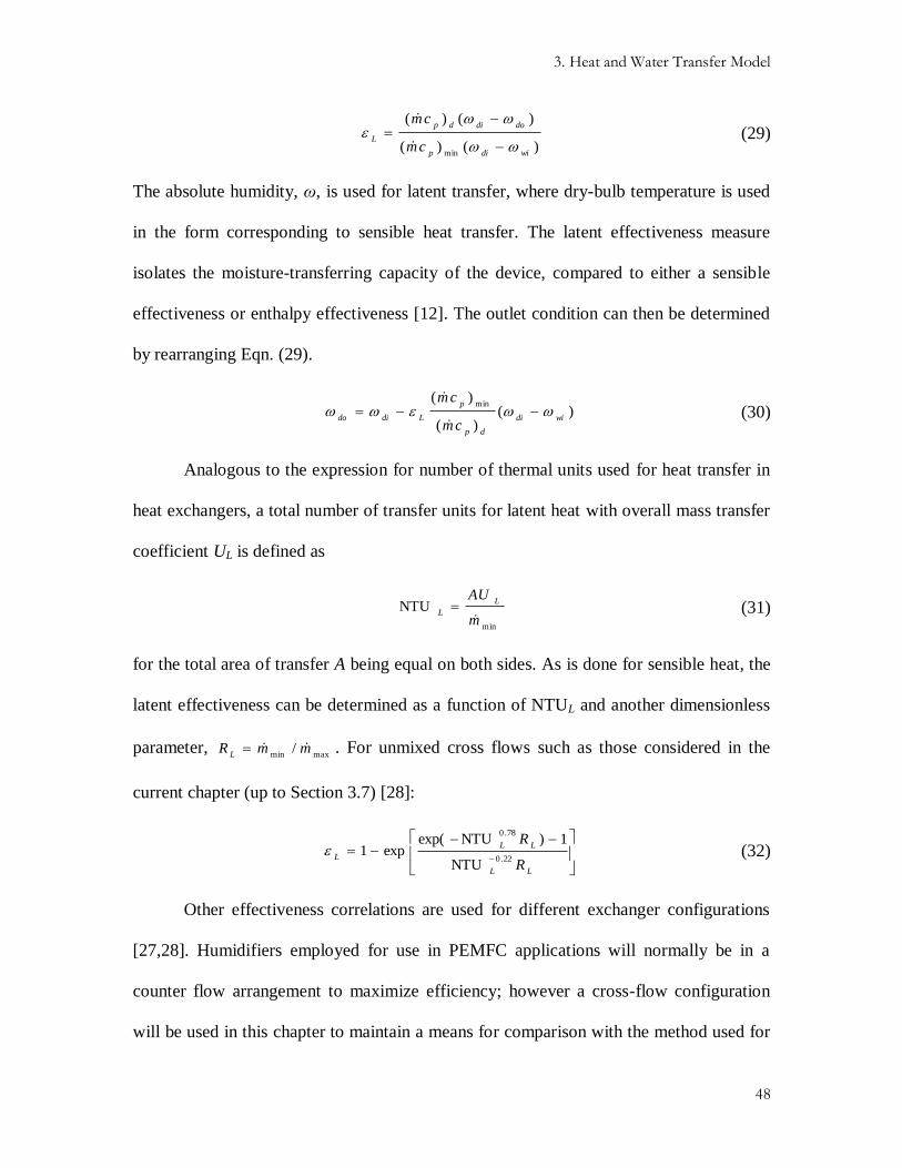
3. Heat and Water Transfer Model

48

)()(

)()(

min widip

dodidp

Lcm

cm

(29)

The absolute humidity, ω, is used for latent transfer, where dry-bulb temperature is used

in the form corresponding to sensible heat transfer. The latent effectiveness measure

isolates the moisture-transferring capacity of the device, compared to either a sensible

effectiveness or enthalpy effectiveness [12]. The outlet condition can then be determined

by rearranging Eqn. (29).

)()(

)(min

widi

dp

p

Ldidocm

cm

(30)

Analogous to the expression for number of thermal units used for heat transfer in

heat exchangers, a total number of transfer units for latent heat with overall mass transfer

coefficient UL is defined as

min

NTUm

AUL

L

(31)

for the total area of transfer A being equal on both sides. As is done for sensible heat, the

latent effectiveness can be determined as a function of NTUL and another dimensionless

parameter, maxmin

/ mmRL

. For unmixed cross flows such as those considered in the

current chapter (up to Section 3.7) [28]:

LL

LL

LR

R

22.0

78.0

NTU

1)NTUexp(exp1 (32)

Other effectiveness correlations are used for different exchanger configurations

[27,28]. Humidifiers employed for use in PEMFC applications will normally be in a

counter flow arrangement to maximize efficiency; however a cross-flow configuration

will be used in this chapter to maintain a means for comparison with the method used for

3. Heat and Water Transfer Model

49

ERVs. The latent effectiveness can therefore be substituted into Eqn. (30) to determine

the outlet moisture content. The total moisture transfer conductance UL has been

calculated by Niu and Zhang.

When considering mass transfer from the wet side to the dry side, diffusion

through the membrane as described by adsorption isotherms can be used to adequately

account for the water transport [45]. Based on the membrane water uptake characteristics

as described by its sorption curve, the water uptake on the dry side in terms of relative

humidity would be:

)(mwmd

mw

mw

mw

mwmd

(33)

Water flux through the membrane at steady state is modeled with Fick’s First Law

for diffusion:

wmOH

Dm2

(34)

According to assumption 1, Eqn. (34) is reduced to the one-dimensional form:

mem

mdmw

wmwmOHt

Dz

Dm

2

(35)

Incorporating membrane water uptake characteristics by substituting Eqn. (33)

into (35) gives:

mdmw

mwmem

wm

OHt

Dm

2

(36)

To obtain the overall mass transfer coefficient UL, the relative humidities must be

changed into the driving force of absolute humidity ω, from a linear relation between the

two parameters. Substituting the Clausius-Clapeyron equation into the relationship

between relative humidity and absolute humidity based on vapor partial pressure, Zhang

3. Heat and Water Transfer Model

50

and Niu (from Simonson and Besant [30]) arrive at the following relation after

substituting for the pressure at standard atmosphere:

61.1

106

/5294

Te

(37)

The second term on the right hand side is ignored in order to simplify the equation

to a linear relationship, assumed to have an effect of less than 5%.

6

/5294

10

Te

(38)

Therefore, Eqn. (36) can now be written in terms of the driving force of absolute

humidity.

mdmw

T

mwmem

wm

OH

e

t

Dm

6

/5294

102

(39)

Assuming steady state operation and equilibrium at the interfaces, the moisture

transfer across the membrane can be written in terms of surface mass transfer resistances:

)()(2 dmdMdmwwMwOH

hhm (40)

The unknown absolute humidities at the membrane can then be eliminated from

Eqn. (39) by first rearranging Eqn. (40).

MwOHwmwhm /

2

(41)

MdOHdmdhm /

2

(42)

Setting the moisture diffusive resistance in the membrane

6

/5294

10

T

mw

wm

mem

m

eD

t

(43)

3. Heat and Water Transfer Model

51

and substituting (41) and (42) into Eqn. (39) and rearranging leads to the water transfer in

terms of the difference in absolute humidity as the driving force:

dw

Md

m

Mw

OHhh

m

1

11

2

(44)

Therefore, the overall mass transfer coefficient UL to be used in Eqn. (31) has

been found as

1

11

Md

m

Mw

Lhh

U (45)

The first and third terms on the right side are the convective mass transfer

resistances as produced with the heat-mass transfer analogy, while the middle term, Eqn.

(43), is analogous to the conduction resistance in heat transfer.

3.4. CURRENT LIMITATIONS OF ε-NTU METHOD FOR MASS TRANSFER

This section discusses the limitations of the ε-NTU method for heat and mass

transfer in membrane humidity exchangers as proposed by L.Z. Zhang in [29],

specifically in the context of applying the same model to PEMFC heat and humidity

exchangers. Two key observations can be made regarding the derivations that call into

question the validity of the ε-NTU method being applied to fuel cell humidifiers:

1. The Clausius-Clapeyron reference temperature (used in the value for constant

enthalpy of vaporization) is a constant and may be far from the actual operating

temperature;

2. At higher temperatures, the absolute humidity calculated without the 1.61 term in

Eqn. (37) will diverge substantially due to the non-linear nature of the saturated water

vapor pressure curve.

3. Heat and Water Transfer Model

52

3.4.1. USE OF THE CLAUSIUS-CLAPEYRON SATURATION VAPOR PRESSURE EQUATION

The Clausius-Clapeyron equation is a theoretical expression for the saturation

vapor pressure of most liquids [46] and provides a direct relation between saturation

pressure and temperature (see next section):

RT

H

RT

HPP

vap

ref

vap

refsatexpexp (46)

The form of Clausius-Clapeyron equation used by Zhang (after Simonson Besant

[30]) employs a reference state of 3007 Pa and 297.3 K (24.1°C) and assumes a constant

heat of vaporization at that state:

T

sateP

/52941110629.1

(47)

A result of assuming a constant heat of vaporization is that the error in the

equation increases with larger deviations from the reference conditions. Figure 3.2 shows

the percent deviation of Eqn. (47) compared to the Hyland-Wexler equation. The well-

known Goff-Gratch equation is also shown for a third reference correlation.

-2%

0%

2%

4%

6%

8%

10%

12%

14%

16%

18%

-20 0 20 40 60 80 100 120

Temperature (°C)

Dev

iati

on

fro

m H

yla

nd

-Wex

ler

Hyland-Wexler

Goff-Gratch

Clausius-Clapeyron (Zhang)

Clausius-Clapeyron (Kadylak)

Figure 3.2: Comparison of saturated vapor pressure from four different equations

3. Heat and Water Transfer Model

53

From a survey of fuel cell system manufacturers’ requirements for backup and

portable power applications, a reference temperature of 50°C is more in line with the

operating conditions experienced in PEM fuel cell humidification, and the corresponding

heat of vaporization results in a saturation vapor pressure equation in the Clausius-

Clapeyron form of:

T

sateP

/50571010731.7

(48)

The Goff-Gratch and Hyland-Wexler equations show very little deviation from

each other and are taken to be most accurate [47], where Goff-Gratch is generally

considered the reference equation. The percent deviation of the Clausius-Clapeyron

equation used by Zhang, Eqn. (47), is within an acceptable 2% for most atmospheric

temperatures, but increases rapidly at either higher or lower temperatures. The Clausius-

Clapeyron equation derived for fuel cell applications, Eqn. (48), has also been plotted,

and it can be seen that the deviation is within 2% for most fuel cell applications from

21°C to 80°C.

3.4.2. CORRELATION BETWEEN ABSOLUTE HUMIDITY AND RELATIVE HUMIDITY

From the definitions of relative humidity and absolute humidity, the following

relation can be derived:

622.0622.0

satP

P (49)

The numeric constant 0.622 is the molecular weight ratio of water to dry air composition.

Substituting in Eqn. (47) for a standard atmospheric pressure of 101,325 Pa this time,

Zhang (after Simonson and Besant [30]) arrived at:

3. Heat and Water Transfer Model

54

622.010

6

/5294

Te

(50)

Zhang (and Simonson and Besant) then neglected the second term on the right

hand side on the grounds that it is generally less than 5% of the first term on the right

hand side. This approximation can be made if the vapor pressure is much less than the air

pressure, and can be arrived at by starting with a simplified version of the definition of

humidity ratio.

airv

v

v

vPP

P

P

PP

P

,622.0622.0 (51)

While this is a reasonable assumption at atmospheric pressures (~1 atm) and temperatures

(20 – 40°C), it is not the case at the higher temperatures that are found in fuel cell

humidifiers (see Figure 3.3). With values up to 20% of the other term at 60°C and 100%

relative humidity, the second term on the right hand side of Eqn. (50) cannot be

neglected. Also, fuel cell operation is not always near atmospheric pressures, so it is

premature to substitute the atmospheric pressure into Eqn. (39) at this point.

0%

10%

20%

30%

40%

50%

60%

0 0.2 0.4 0.6 0.8 1

Relative Humidity

Mag

nit

ud

e of

2n

d t

erm

com

par

ed t

o 1

st o

n R

HS

T = 80°C

70°C

60°C

50°C

40°C

30°C

Figure 3.3: Magnitude of second term compared to first on right hand side of Eqn. (50)

3. Heat and Water Transfer Model

55

3.5. A NEW APPROACH TO USING LATENT EFFECTIVENESS

This section discusses techniques to address the limitations presented above and to

render the ε-NTU method applicable to PEMFC membrane heat and humidity

exchangers. Firstly, the Clausius-Clapeyron equation, Eqn. (46), can still be used, but the

enthalpy of vaporization and reference states shall be calculated at the operating

conditions, and substituted directly into Eqn. (49). As well, the pressure P in Eqn. (49)

will remain a variable parameter.

622.0)/exp(622.0

)/exp(

refvapref

vap

RTHP

RTHP (52)

The use of the Clausius-Clapeyron equation and neglecting the /0.622 term in

Eqn. (50) allow Zhang to provide a simplified expression for overall moisture transfer

resistance across the membrane analogous to the overall heat transfer coefficient. Without

these assumptions, the problem cannot be simplified as easily. The proposed solution is

to maintain the /0.622 term, thereby making the solution iterative. One has the following

system of three flux equations with five unknowns (J, ωmw, θmw, ωmd, and θmd):

dmdMd

mdmw

mem

wm

mwwMw

hJ

t

DJ

hJ

(53)

Introducing two more unknowns (relative humidities on either surface of the

membrane, md and mw) and four equations of relation ( to ω and to θ) close the

problem:

622.0622.0

622.0622.0

,

md

dsatmd

md

mw

sat,wmw

mw

P

P

P

P

(54)

3. Heat and Water Transfer Model

56

where Psat has been left as is, since any saturated water vapor relation can be used, such

as the Hyland-Wexler or Goff-Gratch equation referred to in Section 3.4.1.

The two sorption curves for the membrane under consideration, relating water

uptake θ to relative humidity at the membrane interface are the final two equations and

can be represented parametrically as:

md

md

mw

mw

CC

CC

1

1

max

max

(55)

C is a variable denoting the type of membrane being used because the membrane type

affects the shape of the sorption curve. A value of C = 1 denotes a linear membrane,

usually employing a silica gel desiccant. A Type-I membrane such as a molecular sieve

has a value of C < 1, and Type-III membranes such as those containing polymer

desiccants have a value of C > 1 [32].

This provides a set of seven equations, two of which are non-linear. Since the

problem remains non-linear an iterative approach is required. The proposed solution

further requires determining an effective overall mass transfer coefficient Ueff

)(dweff

UJ (56)

instead of the overall mass transfer coefficient UL found through mass transfer resistances

in Eqn. (45).

The method of determining the humidifier outputs of absolute humidity is as

follows:

Solve the seven non-linear equations (53) to (55) simultaneously to find the flux J;

Find the effective mass transfer coefficient Ueff using Eqn. (56);

3. Heat and Water Transfer Model

57

Use Ueff in place of UL in the equation used to find NTUL, Eqn. (31);

The latent effectiveness is now found from the correlation of Eqn. (32) or similar;

The outputs can now be found from Eqn. (30).

An outside iterative loop must be implemented involving a first estimate for the outlet

values of absolute humidity (ωdo and ωwo), and using subsequent approximations, to

obtain values to use for the absolute humidities in Eqn. (56). The process of solving for

the outlet conditions is presented in the flow chart of Figure 3.4. The model was created

in Mathcad, and the complete details can be found in the Appendix.

Find J by solving

Eqns. (53) – (55)

Initial Tdo, Two,

ωdo, ωwo

Obtain Ueff

Find NTUL

Use correlation to

obtain εL

Obtain new

Tdo, Two, ωdo, ωwo

Subtract initial

Tdo, Two, ωdo, ωwo

< set

tolerance

no

Adjust Tdo, Two,

ωdo, ωwo

Arrive at solution

Tdo, Two, ωdo, ωwo

yes

Figure 3.4: Procedure for solving humidifier outlet conditions

3. Heat and Water Transfer Model

58

3.6. RESULTS OF COMPARISON TO PREVIOUS EFFECTIVENESS METHOD

The solution presented in the previous section was implemented and compared to

the one given by Zhang and Niu. The inputs used for this comparison are summarized in

Table 3.1. The inputs were arrived at by considering typical PEM fuel cell conditions but

also closely following the parameters used by Zhang and Niu in previous work.

Table 3.1: Summary of parameters used in humidifier model comparisons

l 500 mm Dwm 2.16 × 10–8

kg/m ∙ s

B 500 mm θmax 0.23 kg/kg

d 5 mm membrane PVC

w 5 mm configuration cross-flow

M 30 layers di 0 to 0.9 RH

n 83 channels wi 1 RH

m 0.05 kg/s Tdi 70 °C

Q 2350 SLPM Pdi 1 atm

tmem 0.02 mm Twi 70 °C

kmem 0.18 W/m ∙ K Pwi 1 atm

Figure 3.5 compares the new method to that used by Zhang and Niu of NTUL

when varying the dry inlet relative humidities from 0 to 90% for three types of

membrane. While the new method follows similar trends to that of Zhang and Niu for the

corresponding type of membrane, the values in NTUL vary considerably. The differences

are most pronounced for the extreme ranges of dry inlet relative humidities for Type-I

and Type-III membranes, and for the higher relative humidities in linear-type

membranes.

The effect that a change in NTUL has on the latent effectiveness is portrayed

graphically in Figure 3.6. As expected, the curves of effectiveness follow the same shapes

as those for NTUL for each membrane type. The variations between the two methods

employed are of similar magnitude in the εL curves, just as in the NTUL curves.

3. Heat and Water Transfer Model

59

According to Eqn. (30) the difference in effectiveness between the two methods will also

determine how severely the simplifications made by Zhang and Niu affect the outputs,

namely the outlet absolute humidity ωdo, when compared to the inlet absolute humidity

ωdi. Therefore, in an extreme example of 90% relative humidity at the dry inlet for a

linear type membrane operating at the 70°C isothermal case investigated (right side of

Figure 3.5b), the error caused by using the ERV method would translate to a 40% over-

prediction in outlet absolute humidity as compared to the inlet absolute humidity.

Figure 3.5: Variation of NTUL with inlet relative humidity for constant NTU: a) Type-I membrane (C = 0.1); b) linear-type membrane (C = 1); c) Type-III membrane (C = 10)

3. Heat and Water Transfer Model

60

Figure 3.6: Latent effectiveness for constant NTU: a) Type-I membrane (C = 0.1); b) linear-type

membrane (C = 1); c) Type-III membrane (C = 10)

When dealing with PEMFC humidification, the dry inlet stream will generally be

supplied very dry by a compressor or blower creating a dew point of –20°C or lower, or

less than 3% relative humidity. Thus, the points of greatest interest on the curves are at

the far left, at zero dry inlet relative humidity. Table 3.2 summarizes the NTUL and latent

effectiveness deviations when the simplifications made by Zhang and Niu are used as

compared to the proposed solution method of this paper. When the two limitations have

been addressed using the new method, improvement is made to the calculated outputs,

ranging from 23% to 46% difference if using simplifications in the ERV method, for the

Type-III membrane when determining the latent effectiveness for the 70°C isothermal

case.

3. Heat and Water Transfer Model

61

Table 3.2: Comparison based on methodology of latent NTU and latent effectiveness for 0% dry inlet RH

Difference Kadylak-Cave vs. Zhang-Niu

Membrane NTUL εL

Type-I 32.4% 29.1%

linear-type –26.3% –22.7%

Type-III 56.8% 46.4%

As the conditions for PEMFC operation have larger variations from those of

ERVs, it is expected that the difference between effectivenesses found using the two

methods will grow, and it will become more important to implement the approach

outlined in this chapter. Even for ERV studies, implementing these recommendations will

improve outlet condition prediction accuracy.

3.7. EXPERIMENTAL VALIDATION OF MODEL

A proper, complete model requires membrane properties to be defined. A

diffusion coefficient correlation is the only parameter that remains to be determined; so

the diffusion coefficient is treated as a fitted parameter to the data. The temperature

chosen to obtain the diffusion coefficient is 25°C, where there is the most confidence in

the data. For the polymer-hydrophilic additive membrane, the experimental data point

with the least variance occurs at 0.7 SLPM with a standard error of 0.042°C dew point

between samples, whereas for the perfluorinated composite membrane the least variance

occurs at 0.4 SLPM with a standard error of 3.3°C dew point. The diffusion coefficient

for the porous polymer membrane was determined to be Dm = 9.42 × 10–10

m2/s, while for

the ionic membrane the diffusion coefficient was found to be Dm = 6.21 × 10–11

m2/s.

Although the perfluorinated membrane has a smaller diffusion coefficient by a factor of

15, it performs better in terms of water transfer at equal conditions. As a reference, Chen

3. Heat and Water Transfer Model

62

and Peng reported the diffusion coefficient for Nafion 115 (0.127 mm thick) to vary

between 9.12 × 10–11

m2/s and 3 × 10

–10 m

2/s [22].

The diffusion coefficient also needs to be fitted at different temperatures. The

diffusion coefficient as a function of temperature is modeled by an Arrhenius relation

with activation energy Ea, as also found implemented in the literature for Nafion [48]:

mref

a

mwmTTR

EDD

11exp (57)

The reference temperature Tref is 298.15 K, the temperature at which Dm was

found for the first point. Once the temperature dependence of the diffusion coefficient is

applied to the data, as shown in Figure 3.7, the activation energy for the polymer-

hydrophilic additive membrane is found to be 24,300 J/mol.

0

10

20

30

40

50

60

70

80

0 0.2 0.4 0.6 0.8 1 1.2

Air Flow Rate Q air (SLPM)

Dew

Po

int

Tem

per

atu

re

Td

p,d

o (

°C)

Model

Experimental

Figure 3.7: Model comparison to experimental data for porous polymer with hydrophilic additive

membrane, at ♦ Tiso = 25°C, ● 50°C, ■ 75°C

3. Heat and Water Transfer Model

63

Fitting the diffusion coefficient over the range of temperatures for the

perfluorinated composite membrane yields an activation energy of 34,800 J/mol, with the

results in Figure 3.8. Hence, the model is able to agree with the experimental data to

within the experimental error bars corresponding to a 95% confidence interval. Higher

activation energy is required for the ionic membrane than for the porous polymer

membrane, in order to account for the higher water transfer at high temperatures. The

activation energies for these tested membranes are within the vicinity of the activation

energies in the literature for Nafion of 20,096 J/mol [48] and 18,003 J/mol [49]. Chen et

al. also report higher activation energy than Yeo and Eisenberg from their tests with

liquid-to-air membrane humidification [19].

0

10

20

30

40

50

60

70

80

0 0.2 0.4 0.6 0.8 1 1.2

Air Flow Rate Q air (SLPM)

Dew

Po

int

Tem

per

atu

re

Td

p,d

o (

°C)

Model

Experimental

Figure 3.8: Model comparison to experimental data for ionic perfluorinated composite membrane, at ♦

25°C, ● 50°C, ■ 75°C

64

4. CONCLUSIONS

A study on the water transfer performance of humidifiers requires an

understanding of different metrics to quantify humidity transfer. Through experiments

that varied the parameters that affect water transfer, a key finding was that water recovery

ratio is the most appropriate performance metric for fuel cell humidifiers, as it accounts

for the amount of water supplied even as the fuel cell operating conditions may change.

Initial experiments demonstrated that temperature has a greater effect on water

transport than pressure effects over the practical temperature (25°C – 80°C) and pressure

(0 kPag and 120 kPag over 35 kPa pressure difference) operating ranges found in PEM

fuel cells. Temperature had three times the effect compared to pressure on the dry outlet

dew point temperature in the particular tests conducted on a subscale humidifier.

Membrane characterization experiments revealed that the porous and ionic

membranes had similar low water uptake profiles at relative humidities less than 80%,

with the profiles increasing sharply after 80%, but the porous membrane had a higher

maximum water uptake than the ionic membrane. Conversely, the isothermal experiments

conducted in the single cell humidifier with the porous and ionic membranes showed that

the ionic composite membrane had better water transport characteristics than the porous

polymer-hydrophilic additive membrane, ranging from as low as an 11% improvement at

the low temperature, low flow condition up to a 56% improvement at the high flow test

condition.

The extension of sensible heat effectiveness-number of transfer units to conditions

with latent energy transfer is a method for gauging the enthalpy performance of heat and

humidity exchangers. Zhang and Niu have developed a method for determining the latent

4. Conclusions

65

effectiveness and latent number of transfer units from an analogy to heat transfer.

However, limitations were discovered when applying the technique from ERVs to

PEMFC plate-and-frame membrane humidifiers. The two limitations that cause the

predicted outlet conditions to deviate from the true conditions are:

1. The use of a constant enthalpy of vaporization taken from a low reference

temperature in the Clausius-Clapeyron equation;

2. The simplification used in order to make a linear relationship between relative

humidity and absolute humidity.

Using the Clausius-Clapeyron equation with the parameters that Zhang and Niu

use will create a 4% deviation from the Hyland-Wexler equation for the water saturation

pressure curve at 70°C. With the simplification of the vapor pressure being much less

than the air pressure to make the relation between relative humidity and absolute

humidity linear, the absolute humidity value from using the relation can be underreported

by over a third at 70°C.

Due to the elevated temperatures used in PEM fuel cells as compared to ERV

systems and the non-linear dependence of the water saturation curve on temperature, the

aforementioned limitations were addressed in order to use the latent effectiveness method

for PEMFC membrane humidifiers. This was accomplished by finding an effective mass

transfer coefficient Ueff instead of the UL proposed by Zhang and Niu. The Ueff coefficient

is calculated by first iteratively solving the relevant constitutive equations to find the flux

of water through the membrane.

The new procedure was applied to three membrane types (Type I, linear, and Type

III) and compared to the curves of latent effectiveness and latent NTU found using Zhang

4. Conclusions

66

and Niu’s method. In fuel cell operation, the most likely conditions for the incoming wet

and dry streams will be 100% and close to 0% relative humidity, respectively. For a 70°C

isothermal case, the technique yielded an enhancement in latent effectiveness of 29% for

Type-I membranes, 23% for linear-type membranes, and 46% for Type-III membranes as

compared to the ERV method.

Since a straightforward thermodynamic model to predict water transport through a

membrane was developed, there was also the requirement to validate it with experimental

data. Diffusion coefficients were extracted from the experimental data by using an

Arrhenius relation for temperature dependence. The porous polymer membrane had a

diffusion coefficient of 9.42 × 10–10

m2/s, and the ionic perfluorinated membrane had a

diffusion coefficient of 6.21 × 10–11

m2/s. With the appropriate activation energies in the

Arrhenius equation, the model matched the experimental results closely within the 95%

confidence interval experimental error bars, thereby validating the practical use of the

thermodynamic model for the range of conditions tested.

In conclusion, the key findings put forward in this thesis are:

Evaluation of performance metrics, identifying water recovery ratio as the most

appropriate for fuel cell membrane humidifiers;

Characterization of the sorption isotherms, water transfer performance, and

diffusivity of a porous membrane and an ionic membrane, which had the higher

performance;

Development of a thermodynamic membrane humidifier model amenable to PEM

fuel cell conditions based on the heat exchanger effectiveness method; and,

4. Conclusions

67

Corroboration of the heat and mass transfer model with experimental data and

correlated diffusion coefficients.

4.1. FUTURE WORK

The model is ready to be tested to predict performance of commercially available

products, with the caveat that true two-phase flow has not been integrated. As such, it

may serve better as a tool to compare the relative performance of two or more

humidifiers, or to benchmark the performance of an existing humidifier product. The next

steps in further developing the model would be to analyze added complexity, such as

accounting for condensation, and thus two-phase flow. Some additions to the model that

may prove beneficial would be heat transfer to surroundings and the effect of pressure

drop. The effects of pressure difference across the membrane, possibly driving

permeation, and the effect of different total pressures—although incorporated into the

fluid properties of the flows in the model—could also be investigated. The effect of

temperature difference between the two streams, which was not studied because it would

introduce condensation and two-phase flow, is another area for further research. The

interested researcher is directed to Section 2.2, which lays out the parameters that affect

water transfer, for further avenues of investigation that were not covered.

Finally, if different membranes will be used in the model, it is imperative that the

membrane be characterized as to its water uptake. Further experiments will need to be

undertaken to determine the diffusion coefficient, especially as it relates to temperature.

68

REFERENCES

[1] E.J. Carlson, P. Kopf, J. Sinha, S. Sriramulu, Y. Yang, Cost Analysis of PEM Fuel

Cell Systems for Transportation, National Renewable Energy Laboratory Report No.

NREL/SR-560-39104 (Golden, Colorado) (2005) 85-95.

[2] J. Larminie, A. Dicks, Fuel Cell Systems Explained, second ed., John Wiley & Sons,

West Sussex, England, 2003.

[3] N. Rajalakshmi, T.T. Jayanth, R. Thangamuthu, G. Sasikumar, P. Sridhar, K.S.

Dhathathreyan. Water transport characteristics of polymer electrolyte membrane fuel cell,

Int. J. Hydrogen Energy 29(10) (2004) 1009-1014.

[4] W. Merida, D.A. Harrington, J.M. Le Canut, G. McLean. Characterisation of proton

exchange membrane fuel cell (PEMFC) failures via electrochemical impedance

spectroscopy, J. Power Sources 161(1) (2006) 264-274.

[5] W. Merida, Diagnosis of PEMFC stack failures via electrochemical impedance

spectroscopy, Ph.D. Thesis (2002).

[6] S.D. Knights, K.M. Colbow, J. St-Pierre, D.P. Wilkinson. Aging mechanisms and

lifetime of PEFC and DMFC, J. Power Sources 127(1-2) (2004) 127-134.

[7] X. Huang, R. Solasi, Y. Zou, M. Feshler, K. Reifsnider, D. Condit, et al. Mechanical

endurance of polymer electrolyte membrane and PEM fuel cell durability, J. Polym. Sci.

B 44(16) (2006) 2346-2357.

[8] H. Tang, S. Peikang, S.P. Jiang, F. Wang, M. Pan. A degradation study of Nafion

proton exchange membrane of PEM fuel cells, J. Power Sources 170(1) (2007) 85-92.

[9] M.B. Satterfield, J.B. Benziger. Non-Fickian water vapor sorption dynamics by

Nafion membranes, J. Phys. Chem. B 112(12) (2008) 3693-3704.

[10] M.B. Satterfield, P.W. Majsztrik, H. Ota, J.B. Benziger, A.B. Bocarsly. Mechanical

properties of Nafion and titania/Nafion composite membranes for polymer electrolyte

membrane fuel cells, J. Polym. Sci. B 44(16) (2006) 2327-2345.

[11] D.M. Bernardi. Water-balance calculations for solid-polymer-electrolyte fuel cells, J.

Electrochem. Soc. 137(11) (1990) 3344-3350.

[12] P. Cave, W. Merida. Water flux in membrane fuel cell humidifiers: flow rate and

channel location effects, J. Power Sources 175(1) (2008) 408-418.

[13] R. Huizing, M. Fowler, W. Mérida, J. Dean. Design methodology for membrane-

based plate-and-frame fuel cell humidifiers, J. Power Sources 180(1) (2008) 265-275.

References

69

[14] F.N. Büchi, S. Srinivasan. Operating proton exchange membrane fuel cells without

external humidification of the reactant gases, J. Electrochem. Soc. 144(8) (1997) 2767-

2772.

[15] D.P. Wilkinson, H.H. Voss, K. Prater. Water management and stack design for solid

polymer fuel cells, J. Power Sources 49(1-3) (1994) 117-127.

[16] Y.A. Çengel, M.A. Boles, Thermodynamics: An Engineering Approach, fourth ed.,

McGraw-Hill, Boston, 2002.

[17] R.A. Parsons, ASHRAE Handbook: HVAC Systems and Equipment, American

Society of Heating, Refrigerating and Air-Conditioning Engineers, Atlanta, Ga., 1996,

ch. 42.

[18] P.W. Majsztrik, M.B. Satterfield, A.B. Bocarsly, J.B. Benziger. Water sorption,

desorption and transport in Nafion membranes, J. Membr. Sci. 301(1) (2007) 93-106.

[19] D. Chen, W. Li, H. Peng. An experimental study and model validation of a

membrane humidifier for PEM fuel cell humidification control, J. Power Sources 180(1)

(2008) 461-467.

[20] S. Park, I.-H. Oh. An analytical model of NafionTM

membrane humidifier for proton

exchange membrane fuel cells, J. Power Sources 188(2) (2009) 498-501.

[21] S.-K. Park, S.-Y. Choe, S.-H. Choi. Dynamic modeling and analysis of a shell-and-

tube type gas-to-gas membrane humidifier for PEM fuel cell applications, Int. J.

Hydrogen Energy 33(9) (2008) 2273-2282.

[22] D. Chen, H. Peng. A thermodynamic model of membrane humidifiers for PEM fuel

cell humidification control, J. Dyn. Sys., Meas., Control 127(3) (2005) 424-432.

[23] G. Hoogers, Fuel Cell Technology Handbook, CRC Press, Boca Raton, Fla., 2003, p.

4.13.

[24] C.W. Monroe, T. Romero, W. Mérida, M. Eikerling. A vaporization-exchange

model for water sorption and flux in Nafion, J. Membr. Sci. 324(1-2) (2008) 1-6.

[25] R. Huizing, Design and membrane selection for gas to gas humidifiers for fuel cell

applications, M.A.Sc. Thesis (2007).

[26] P. Cave, Membrane moisture transfer in fuel cell humidifiers, M.A.Sc. Thesis

(2007).

[27] W.M. Kays, A.L. London, Compact Heat Exchangers, second ed., McGraw-Hill,

New York, 1964.

[28] F.P. Incropera, D.P. DeWitt, Fundamentals of Heat and Mass Transfer, fifth ed.,

John Wiley & Sons, Toronto, 2002.

References

70

[29] L. Zhang, J.L. Niu. Effectiveness correlations for heat and moisture transfer

processes in an enthalpy exchanger with membrane cores, J. Heat Transfer 124(5) (2002)

922-929.

[30] C.J. Simonson, R.W. Besant. Energy wheel effectiveness: part I--development of

dimensionless groups, Int. J. Heat Mass Transfer 42(12) (1999) 2161-2170.

[31] L. Zhang, Y. Jiang. Heat and mass transfer in a membrane-based energy recovery

ventilator, J. Membr. Sci. 163(1) (1999) 29-38.

[32] J.L. Niu, L. Zhang. Membrane-based enthalpy exchanger: material considerations

and clarification of moisture resistance, J. Membr. Sci. 189(2) (2001) 179-191.

[33] S.-K. Park, E.A. Cho, I.-H. Oh. Characteristics of membrane humidifiers for

polymer electrolyte membrane fuel cells, Korean J. Chem. Eng. 22(6) (2005) 877-881.

[34] Vaisala, Vaisala HUMIDICAP® Humidity and Temperature Transmitter Series

HMT330 User's Guide, Vaisala Oyj, Helsinki, 2005, ch. 7.

[35] M. Asaeda, L.D. Du. Separation of alcohol/water gaseous mixtures by thin ceramic

membrane, J. Chem. Eng. Jpn. 19(1) (1986) 72-77.

[36] P.W. Gibson. Effect of Temperature on water vapor transport through polymer

membrane laminates, Polym. Test. 19(6) (2000) 673-691.

[37] J. Crank, G.S. Park, Diffusion in Polymers, Academic Press, New York, 1968, p.

452.

[38] D.J. Burnett, A.R. Garcia, F. Thielmann. Measuring moisture sorption and diffusion

kinetics on proton exchange membranes using a gravimetric vapor sorption apparatus, J.

Power Sources 160(1) (2006) 426-430.

[39] C.J. Simonson, R.W. Besant. Energy wheel effectiveness: part II--correlations, Int. J.

Heat Mass Transfer 42(12) (1999) 2171-2185.

[40] R.H. Perry, D.W. Green, Perry's Chemical Engineers' Handbook, seventh ed.,

McGraw-Hill, Toronto, 1997, p. 12.34.

[41] P. Choi, N. Jalani, R. Datta. Thermodynamics and proton transport in Nafion II.

Proton diffusion mechanisms and conductivity, J. Electrochem. Soc. 152(3) (2005) 123-

130.

[42] T.A.J. Zawodzinski, M. Neeman, L.O. Sillerud, S. Gottesfeld. Determination of

water diffusion coefficients in perfluorosulfonate ionomeric membranes, J. Phys. Chem.

95(15) (1991) 6040-6044.

[43] F.M. White, Heat and Mass Transfer, rev. ed., Addison-Wesley, Don Mills, Ontario,

1988, p. 586.

References

71

[44] D. Kadylak, P. Cave, W. Merida. Effectiveness correlations for heat and mass

transfer in membrane humidifiers, Int. J. Heat Mass Transfer 52(5-6) (2009) 1504-1509.

[45] S.-H. Chen, R.-C. Ruaan, J.-Y. Lai. Sorption and transport mechanism of gases in

polycarbonate membranes, J. Membr. Sci. 134(2) (1997) 143-150.

[46] K. Laidler, J. Meiser, Physical Chemistry, Benjamin/Cummings Publishing, Don

Mills, Ontario, 1982, ch. 5.2.

[47] C.J. Gibbins. A survey and comparison of relationships for the determination of the

saturation vapour pressure over plane surfaces of pure water and of pure ice, Ann.

Geophys. 8(12) (1990) 859-885.

[48] S.C. Yeo, A. Eisenberg. Physical properties and supermolecular structure of

perfluorinated ion-containing (Nafion) polymers, J. Appl. Polym. Sci. 21(4) (1977) 875-

898.

[49] M.W. Verbrugge, E.W. Schneider, R.S. Conell, R.F. Hill. The effect of temperature

on the equilibrium and transport properties of saturated poly(perfluorosulfonic acid)

membranes, J. Electrochem. Soc. 139(12) (1992) 3421-3428.

[50] J.H. Keenan, J. Kaye, Gas Tables: thermodynamic properties of air, products of

combustion and component gases, compressible flow functions, John Wiley & Sons, New

York, 1948.

[51] Van Wylen, Gordon John, R.E. Sonntag, C. Borgnakke, Fundamentals of Classical

Thermodynamics, fourth ed., John Wiley & Sons, New York, 1994.

72

APPENDIX: DOCUMENTED MATHCAD MODEL

[:= assigns a value to a variable or defines a formula]

Highlighted fields are for user inputs.

Apply ε-NTU for heat transfer first.

Define geometry.

l := 135∙mm ―average length of channel‖

B := 30∙mm ―width of plate‖

w := 3∙mm ―width of channel‖

n := 7 ―number of channels per plate‖

d := 1∙mm ―depth or thickness of plate, membrane to membrane‖

M := 2 ―number of layers or plates‖

Ak := l∙B Ak = 0.004 m2

Acs := w∙d Acs = 3 × 10–6

m2 ―cross-sectional area‖

A := w∙l A = 4.05 × 10–4

m2

Ac := A + 2∙l∙d Ac = 6.75 × 10–4

m2 ―2 ½-walls of each stream‖

Ah := Ac Ah = 6.75 × 10–4

m2 ―equal heat transfer areas‖

Pwet := 2∙(w + d) Pwet = 0.008 m ―wetted perimeter‖

wet

cs

hP

AD

4: Dh = 1.5 mm ―hydraulic diameter‖

Membrane properties (for porous polymer with hydrophilic additive) and characteristics.

tmem := 0.18 mm ρmem := 0.7∙940∙kg/m3 kmem := 0.48∙W/m∙K

Sorption curve for porous polymer with hydrophilic additive, PFSA coated both sides:

Appendix: Documented Mathcad Model

73

C := 148 umax := 2.5 := 0.005,0.01..1

318.0

37.0

1793.0

0014.0

:G ―coefficients for third-degree polynomial fit of sorption curve‖

3

4

2

321

max

max,

/1,8.0,,1:

GGGG

CC

uifuifu

Diffusion coefficient will be fitted to one test run at one flow rate and checked vs. rest.

Dm := 9.42∙10–10

∙m2/s

Air properties at 1 atm [50]:

[create look-up matrices of temperature Tair (1 atm∙K/1 bar) and enthalpy hair (J/kg)]

ha(temp) := linterp(Tair,hair,temp) ―Mathcad function to interpolate enthalpy‖

T

PTP

air

)KJ/kg05.287(

:, ―ideal gas state equation for density‖

Kkg

J946623.00022.01067.2:

23

6

K

T

K

T

K

TTc

pair

2

68

2

11

m

sN10103.110717.6101.3:

K

T

K

TT

air

Km

W0162.010557.2104.510333.5:

4

2

7

3

10

K

T

K

T

K

TTk

air

s

m108.5101.5104.1:

2

68

2

10

K

T

K

TT

air

Saturated water properties at 1 bar [51]:

[create look-up matrices of temperature T (°C); pressure P (Pa); liquid enthalpy hf (J/kg);

enthalpy of evaporation hfg (J/kg); vapor density ρv (kg/m3); liquid density ρl (kg/m

3)]

Appendix: Documented Mathcad Model

74

Psat(temp) := linterp(T,P,temp) Tsat(press) := linterp(P,T,press)

hw(temp) := linterp(T,hf,temp) hv(temp) := linterp(T,hfg,temp)

hg(temp) := hw(temp) + hv(temp) ρg(temp) := linterp(T, ρv,temp)

Kkg

J958.1001039.010952.210778.1:

2

6

3

9

K

T

K

T

K

TTc

pg

2

78

m

sN10933.910608.3:

K

TT

g

Km

W101695.2:

18362.1

5

K

TTk

g

s

m10038.110264.11043.1:

2

79

2

12

K

T

K

TT

g

Cold and hot stream flow rates.

MnQ

c

2

min

L4.0:

s

m105238.9

3

7

cQ ―cold (dry) side flow rate‖

m'c := ρair(1∙atm,273.15∙K)∙Qc m'c = 1.2307 × 10–6

kg/s ―at STP‖

chQQ :

s

m105238.9

3

7

hQ ―hot (wet) side flow rate‖

m'h := ρair(1∙atm,273.15∙K)∙Qh m'h = 1.2307 × 10–6

kg/s ―at STP‖

First guess for use in dry (cold) fluid properties, iteratively adjust cyan highlighted

values.

T1 := 75 °C P1 := 1∙atm ―absolute‖ 1 := 0.0016 ―known inputs‖

T2 := 75 °C P2 := 1∙atm ―absolute‖ 2 := 0.508 ―first guesses‖

Converting given conditions to humidity ratio.

Appendix: Documented Mathcad Model

75

)(

)(622.0:

111

11

1TPP

TP

sat

sat

ω1 = 3.7914 × 10

–4 ―kg water/kg dry air‖

)(

)(622.0:

222

22

1TPP

TP

sat

sat

ω2 = 0.1492 ―kg water/kg dry air‖

Work out average properties of humid air for dry (―cold‖) side.

2,1min:

21

c

c = 0.2548 ―average RH based on inlet 1 and outlet 2‖

2:

21TT

Tc

Tc = 75 °C ―average temperature of dry (cold) stream‖

2:

21PP

Pc

Pc = 1.0132 × 10

5 Pa ―average pressure of dry stream‖

Pvc := c∙Psat(Tc) Pvc = 9829.6744 Pa ―vapor pressure of dry (cold) stream‖

vcc

vc

cPP

P

622.0: ωc = 0.0668 ―kg water/kg dry air‖

c

c

cx

1: xc = 0.0626 ―mass fraction of water vapor‖

1

),(

1

)(atm1:

ccair

c

cg

cc

cTP

x

T

xP

3m

kg8451.0

c

cpc := xc∙cpg(Tc) + (1 – xc)∙cpair(Tc) cpc = 945.8311 J/kg∙K

μc := xc∙μg(Tc) + (1 – xc)∙μair(Tc) μc = 2.0157 × 10–5

kg/s∙m

kc := xc∙kg(Tc) + (1 – xc)∙kair(Tc) kc = 0.0294 W/m∙K

αc := xc∙αg(Tc) + (1 – xc)∙αair(Tc) αc = 2.7123 × 10–5

m2/s

74.12

5

K15.273

atm1

s

m103.2:

c

c

ABc

T

PD

s

m10508.3

2

5

ABcD from [43]

Appendix: Documented Mathcad Model

76

ccs

hc

cA

Dm

':Re Rec = 30.5293 ―Re < 2300, therefore laminar flow‖

First guess for use in wet (hot) fluid properties, iteratively adjust cyan highlighted values.

T3 := 75 °C P3 := 1∙atm ―absolute‖ 3 := 1 ―known inputs‖

T4 := 75 °C P4 := 1∙atm ―absolute‖ 4 := 0.647 ―first guesses‖

Converting given conditions to humidity ratio.

)(

)(622.0:

333

33

3TPP

TP

sat

sat

ω3 = 0.3824 ―kg water/kg dry air‖

)(

)(622.0:

444

44

4TPP

TP

sat

sat

ω4 = 0.2033 ―kg water/kg dry air‖

Work out average properties of humid air for wet (―hot‖) side.

2,1min:

43

h

h = 0.8235 ―average RH based on inlet 3 and outlet 4‖

2:

43TT

Th

Th = 75 °C ―average temperature of wet (wet) stream‖

2:

43PP

Ph

Ph = 1.0132 × 10

5 Pa ―average pressure of wet stream‖

Pvh := h∙Psat(Th) Pvh = 3.1769 × 104 Pa ―vapor pressure of wet (hot) stream‖

vhh

vh

hPP

P

622.0: ωh = 0.2841 ―kg water/kg dry air‖

h

h

hx

1: xh = 0.2212 ―mass fraction of water vapor‖

1

),(

1

)(atm1:

hhair

h

hg

hh

hTP

x

T

xP

3m

kg5946.0

h

cph := xh∙cpg(Th) + (1 – xh)∙cpair(Th) cph = 786.1145 J/kg∙K

Appendix: Documented Mathcad Model

77

μh := xh∙μg(Th) + (1 – xh)∙μair(Th) μh = 1.8704 × 10–5

kg/s∙m

kh := xh∙kg(Th) + (1 – xh)∙kair(Th) kh = 0.0282 W/m∙K

αh := xh∙αg(Th) + (1 – xh)∙αair(Th) αh = 2.2562 × 10–5

m2/s

74.12

5

K15.273

atm1

s

m103.2:

h

h

ABh

T

PD

s

m10508.3

2

5

ABhD from [43]

hcs

hh

hA

Dm

':Re Reh = 32.9013 ―Re < 2300, therefore laminar flow‖

For laminar, fully developed flow and uniform surface heat flux (not uniform surface

temperature), Nusselt number Nu is constant, and for a channel of aspect ratio w/d the

heat transfer coefficient is given by [43]:

h

c

cD

k

d

w

d

wh

82.2772.00391.0:

2

Km

W7316.93

2

c

h

(Assumes heat flux from all walls surrounding cold channels.)

h

h

hD

k

d

w

d

wh

82.2772.00391.0:

2

Km

W8109.89

2

h

h

(Not much different than hc, so it is assumed that T4 is not important.)

For the side-walls of the ribs treated as fins [27,28]:

trib := 1.5∙mm ―thickness/width of ribs (lands)‖

5.0

)(

)(2:

ltk

lthm

ribmem

ribc

fc

m

10873.513

fcm

dm

dm

fc

fc

fc

5.0

)5.0tanh(: ηfc = 0.9786 ―dry fin efficiency‖

5.0

)(

)(2:

ltk

lthm

ribmem

ribh

fh

m

12415.502

fhm

Appendix: Documented Mathcad Model

78

dm

dm

fh

fh

fh

5.0

)5.0tanh(: ηfh = 0.9795 ―wet fin efficiency‖

The temperature ineffectiveness of an extended surface area is found from:

fc

c

ocAn

dln

1

2)1(1: ηoc = 0.9786 ―overall efficiency‖

fh

h

ohAn

dln

1

2)1(1: ηoh = 0.993 ―overall efficiency‖

The overall heat transfer U coefficient is then:

1

1:

hohh

c

kmem

cmem

cochA

A

Ak

At

hU

Km

W4063.45

2

U

(Not much different from 0.5h, so membrane conductivity kmem is negligible.)

This is for a gas to gas heat exchanger and specific heat of air does not change much, so

the heat capacity rates Cc and Ch are close to the same [28].

Cc := m'c∙cpc Ch := m'h∙cph

Cmin := min(Cc,Ch) Cmin = 9.6751 × 10–4

m2∙kg/K∙s

3

Cmax := max(Cc,Ch) Cmax = 0.0012 m2∙kg/K∙s

3

min

:NTUC

AUc

NTU = 31.6786

max

min:

C

CC

r Cr = 0.8311

Assuming that the effectiveness relation for plate and frame is the same as for concentric

tube heat exchangers, then for counter flow [27,28]:

)]1(NTUexp[1

)]1(NTUexp[1,

NTU1

NTU,1:

rr

r

rCC

CCif ε = 0.9992

q := ε∙Cmin∙(T3 –T1) q = 0 W ―heat transfer‖

Appendix: Documented Mathcad Model

79

cC

qTT

12: T2 = 75 °C ―converge with initial value‖

hC

qTT

34: T4 = 75 °C ―converge with initial value‖

The pinch point, or dry bulb approach temperature, is:

DBAT := T3 – T2 DBAT = 0 K

Apply the εL-NTUL method for latent (moisture) transfer.

Using the Chilton-Colburn Analogy to find the dry and wet mass transfer coefficients hM,

where Le = α/DAB:

3/1

:

ABc

c

pc

c

McDc

hh

2ms

kg091.0

Mch

3/1

:

ABh

h

ph

h

MhDc

hh

2ms

kg0986.0

Mhh ―relatively similar result to hMc‖

2:

hc

m

TTT

Tm = 348.15 K ―assume average membrane temp.‖

2:

hc

m

m = 0.5392 ―average membrane water content‖

2:

hc

m

ωmh := ωh ωmc := ωc

Since the gradient in the flux equation is uptake (kg water/kg membrane), need to

multiply diffusion coefficient by ρmem:

Ea := 24300∙J/mol R := 8.3145∙J/mol∙K

m

a

mmemwmTR

EDD

1

K15.298

1exp:

ms

kg105332.2

6

wmD

Initialize variables for solver:

Appendix: Documented Mathcad Model

80

mc := 0.1 mh := 0.9 J := hmh∙(ωh – ωmh) J = 0 kg/s∙m2

mc

mcCC

uu

/1:

max

umc = 0.0019

mh

mhCC

uu

/1:

max

umh = 0.1433

Given

J – hmc∙(ωc – ωmc) == 0 J – Dwm∙(umh – ωmc)/tmem == 0 J – hmh∙(ωmh – ωh) == 0

0622.0)(622.0

mc

csat

c

mc

mc

TP

P

0

622.0)(622.0

mh

hsat

h

mh

mh

TP

P

umc – u(mc) == 0 umh – u(mh) == 0

mhmhmhmcmcmc

mw

mw

mw

md

md

md

uuJFind

u

u

J

,,,,,,:

'

'

'

'

'

'

'

0294.0

2766.0

0732.0

0707.0

8117.0

2782.0

'

'

'

'

'

'

mw

mw

mw

md

md

md

u

u

Check: J – hmh∙(ωh – ωmh) = 0 kg/m2∙s J' = 5.8168 × 10

–4 kg/m

2∙s

The effective overall mass transfer coefficient Ueff according to the new method is then:

ch

eff

JU

':

sm

kg0027.0

2

eff

U

m'min := min(m'c,m'h) m'min = 1.231 × 10–6

kg/s

m'max := max(m'c,m'h) m'max = 1.231 × 10–6

kg/s

min'

:NTUm

UAeff

L

NTUL = 0.881

max

min

'

':

m

mR

L RL = 1

Latent effectiveness:

)]1(NTUexp[1

)]1(NTUexp[1,

NTU1

NTU,1:

LLL

LL

L

L

LLRR

RRif εL = 0.4684

Appendix: Documented Mathcad Model

81

13

min

12:

c

LC

C ω2 = 0.1491 ―kg water/kg dry air‖

13

min

34:

h

LC

C ω4 = 0.2035 ―kg water/kg dry air‖

)()622.0(:

22

22

2TP

P

sat

2 = 0.508 ―converge with initial value‖

)()622.0(:

44

44

4TP

P

sat

4 = 0.647 ―converge with initial value‖

Convert relative humidities to dew point temperatures.

Tdp2 := Tsat(2∙Psat(T2)) Tdp2 = 59.583 °C Psat(Tdp2) = 0.1959 bar

Tdp3 := Tsat(3∙Psat(T3)) Tdp3 = 75 °C

Tdp4 := Tsat(4∙Psat(T4)) Tdp4 = 64.9449 °C

The water flux at the dry outlet is:

A

mJ

c')(

:12

2

sm

kg105194.4

2

4

2

J

m'H2O := (ω2 – ω 1)∙m'c m'H2O = 1.8303 × 10–7

kg/s

The dew point approach temperature is then:

DPAT := Tdp3 – Tdp2 DPAT = 15.4173 K

Finally, the recommended method to quantify the water transport performance is through

the water recovery ratio.

h

c

m

m

'

')(:WRR

3

12

WRR = 0.3889