Effective Features of Algorithm Visualizations · Effective Features of Algorithm Visualizations...
133
Effective Features of Algorithm Visualizations Purvi Saraiya Thesis submitted to the Faculty of the Virginia Polytechnic Institute and State University in partial fulfillment of the requirements for the degree of Master of Science in Computer Science Dr. Clifford A. Shaffer, Chair Dr. Scott McCrickard Dr. Chris North July, 2002 Blacksburg, Virginia Keywords: Algorithm Visualization, Education, Pedagogical Effectiveness, Copyright 2002, Purvi Saraiya
Transcript of Effective Features of Algorithm Visualizations · Effective Features of Algorithm Visualizations...

Effective Features of Algorithm Visualizations
Purvi Saraiya
Thesis submitted to the Faculty of the Virginia Polytechnic Institute and State University
in partial fulfillment of the requirements for the degree of
Master of Science in
Computer Science
Dr. Clifford A. Shaffer, Chair Dr. Scott McCrickard
Dr. Chris North
July, 2002 Blacksburg, Virginia
Keywords: Algorithm Visualization, Education, Pedagogical Effectiveness,
Copyright 2002, Purvi Saraiya

Effective Features of Algorithm Visualizations
Purvi Saraiya
(Abstract)
Current research suggests that by actively involving students, you can increase
pedagogical value of algorithm visualizations. We believe that a pedagogically successful
visualization, besides actively engaging participants, also requires certain other key
features. We compared several existing algorithm visualizations for the purpose of
identifying features that we believe increase the pedagogical value of an algorithm
visualization. To identify the most important features from this list, we conducted two
experiments using a variety of the heapsort algorithm visualizations.
The results of these experiments indicate that the single most important feature is the
ability to control the pace of the visualization. Providing a good data set that covers all
the special cases is important to help students comprehend an unfamiliar algorithm. An
algorithm visualization having minimum features that focuses on the logical steps of an
algorithm is sufficient for procedural understanding of the algorithm. To have better
conceptual understanding, additional features (like an activity guide that makes students
cover the algorithm in detail and analyze what they are doing, and pseudocode display of
an algorithm) may prove to be helpful, but that is a much harder effect to detect.

iii
Acknowledgements
I am very grateful to my advisor Dr. Clifford A. Shaffer for providing me valuable
guidance, support and motivation throughout my thesis. I am also very grateful to Dr.
Scott McCrickard and Dr. Chris North (co-advisors) for their help in defining my thesis
topic and giving me guidance along with Dr. Shaffer. I am also very thankful to Mr.
William McQuain and Dr. Todd Stevens but for whose help, I would have never been
able to conduct my research experiments.
A very special thanks to Dr. Scott McCrickard, his insight and guidance led to
successful conduction of the second experiment of this thesis.
Above all, I thank my parents and my grandmother without whom I would be
nothing.

iv
Contents
1. Introduction ……………………………………………………… 1
2. Literature Review . ……………………………………………………. 5 2.1 Algorithm Visualizations ………………………………….……. 5
2.1.1 BALSA ……………………………………………. 5 2.1.2 Tango and Xtango ………………………………….. 6 2.1.3 GAIGS ……………………………………………. 7 2.1.4 DynaLab ………………………………………………... 7 2.1.5 SWAN …………………………………………………. 8 2.1.6 JAWAA ……………………………………………….… 9 2.1.7 FLAIR ………………………………………………… 9 2.1.8 POLKA ………………………………………………… 10 2.1.9 Samba …….………………………………………….. 11 2.1.10 Mocha ……….………………………………………… 12 2.1.11 HalVis ………………………………………………….. 12 2.1.12 Summary on the capabilities of Algorithm Visualizations 14
2.2 Algorithm Visualization Effectiveness …………………………. 15
3. Creating Effective Visualizations …………………………………….. 18 3.1 Review of Visualizations ……………………………………….. 18 3.2 List of Features ……….…………………………………………. 23
4. Experiment 1 …………………………………………………………. 28 4.1 Procedure …………………………………………………………. 28 4.2 Hypothesis ………………………….…………………………….. 32 4.3 Results ……………………….……………………………………. 32
4.3.1 Total Performance ………………………………………. 32 4.3.2 Individual Question Analysis ……………….……………. 33 4.3.3 GPA vs. Performance ……..……………………………... 35
4.4 Conclusions ……………………………………………………… 36
5. Experiment 2 …………………………………………………….………. 39 5.1 Procedure …………………………………………………………. 39 5.2 Hypothesis ………………………………………………….…….. 44 5.3 Results ……………………………………………………………. 45
5.3.1 Total Performance ……………..…………………………. 45 5.3.2 Individual Question Analysis ……………..…………….. . 47 5.3.3 Performance vs. Learning Time ………..……………….. . 51 5.3.4 GPA vs. Performance …………..……………………….. . 54 5.3.5 Example Usage ………………………..…………………. 55 5.3.6 History (Back Button) Usage ……………..…………….. . 57 5.3.7 Subjective Satisfaction …………….………………… 58

v
5.4 Conclusions ……………………………………………………... .. 59
6. Algorithm Visualizations …………………..…………………………… 61 6.1 Graph Traversals …………………………………..……………… 61 6.2 Skip Lists ………..………………………………………………… 67 6.3 Memory Management (Buffer Pool Applet) ……………..………. 69 6.4 Hash Algorithms ……………..…………………………………… 72 6.5 Collision Resolution Applet ………..………………………….…. 76
7. Conclusions and Future Work ………………..…………………………. 80 7.1 Conclusions ………………………………………………………. 80 7.2 Future Work ……………………………………………………… 81
Bibliography ………………………………………………………………. 84
Appendix A …………………………………………………………………. 88 A.1 Guide 1 …..…………………………………………………….. 88 A.2 Guide 2 ………………..……………………………………….. 89 A.3 Question Set 1 ……..…………………………………………….. 94 A.4 Question Set 2 …………………………..……………………….. 102 A.5 Anova Analysis For Experiment 1 ………………………….…… 111 A.6 Anova Analysis For Experiment 2 ………………….…………… 118
Vita ……………………………………………………………………... 125

vi
List of Figures
Figure 3.1 Heapsort Visualization 1 …….…………………………………… 19 Figure 3.2 Heapsort Visualization 2 ……. …………………………………… 20 Figure 3.3 Heapsort Visualization 3 ……. …………………………………… 21 Figure 3.4 Heapsort Visualization 4 ……. …………………………………… 22 Figure 3.5 Heapsort Visualization 5 …… …………………………………… 23
Figure 4.1 Heapsort Version 1 …………..…………………………………… 29 Figure 4.2 Heapsort Version 2 …………..…………………………………… 30 Figure 4.3 Heapsort Version 3 …………..…………………………………… 30 Figure 4.4 Average performance of participants ……………………………. 33 Figure 4.5 Average performance of participants on Q7 …………………….. 34 Figure 4.6 Average performance of participants on Q8 …………………….. 34 Figure 4.7 Average performance of participants on Q10-13 ………………… 35 Figure 4.8 Scatter plot of GPA vs. Total performance of participants ……… 36
Figure 5.1 Heapsort Verison 1 ……………………………………………….. 40 Figure 5.2 Heapsort Version 2 ………………………………………………. 41 Figure 5.3 Heapsort Version 3 ………………………………………………. 42 Figure 5.4 Heapsort Version 4 ………………………………………………. 42 Figure 5.5 Average performance of participants of each version …………… 46 Figure 5.6 Partial ordering on total performance of participants of each version 47 Figure 5.7 Average performance on conceptual questions …………………... 48 Figure 5.8 Average performance on procedural questions …………………... 48 Figure 5.9 Average performance of the participants on Q 6-8 ……………… 49 Figure 5.10 Average performance of the participants on Q 9-13 …………….. 49 Figure 5.11 Average performance of participants on Q14-16 ……………….. 50 Figure 5.12 Average performance on participants on Q17-24 ……………….. 50 Figure 5.13 Average learning time vs. average scores ……………………….. 52 Figure 5.14 Scatter plot of learning time vs. performance for Version 1 …….. 52 Figure 5.15 Scatter plot of learning time vs. performance for Version 2 ……... 53 Figure 5.16 Scatter plot of learning time vs. performance for Version 3 ……... 54 Figure 5.17 Scatter plot of learning time vs. performance for Version 4 ……... 54 Figure 5.18 Scatter plot of GPA vs. total scores ……………………………... 55 Figure 5.19 Scatter plot of example usage vs. total scores for Version 2 …….. 56 Figure 5.20 Scatter plot of example usage vs. total scores for Version 3 …….. 56 Figure 5.21 Scatter plot of Back button usage vs. total scores for Version 2 …. 57 Figure 5.22 Scatter plot of Back button usage vs. total scores for Version 3 …. 58 Figure 5.23 Average subjective satisfaction for each version ………………… 58

vii
Figure 6.1 Graph Traversal Applet Visualization1 ….. …………………….. 61 Figure 6.2 Graph Traversal Applet Visualization2 ..…. …………………….. 62 Figure 6.3 Graph Traversal Applet Visualization3 ..…. …………………….. 62 Figure 6.4 Graph Traversal Applet Visualization4 …... …………………….. 63 Figure 6.5 Graph Traversal Applet Visualization5 ..…. …………………….. 64 Figure 6.6 Graph Traversal Applet Visualization6 ..…. …………………….. 64 Figure 6.7 Graph Traversal Applet Visualization7 …... …………………….. 65 Figure 6.8 Graph Traversal Applet Visualization8 …... …………………….. 65 Figure 6.9 Skip List Applet Visualization 1 ………………………………… 67 Figure 6.10 Skip List Applet Visualization 1 ………………………………… 68 Figure 6.11 Skip List Applet Visualization 1 ………………………………… 68 Figure 6.12 Memory Management Applet Visualization 1 ………………….. 70 Figure 6.13 Memory Management Applet Visualization 2 ………………….. 70 Figure 6.14 Memory Management Applet Visualization 3 ………………….. 71 Figure 6.15 Memory Management Applet Visualization 4 ………………….. 71 Figure 6.16 Hash Algorithm Applet Visualization 1 …………………………. 72 Figure 6.17 Hash Algorithm Applet Visualization 2 …………………………. 73 Figure 6.18 Hash Algorithm Applet Visualization 3 …………………………. 73 Figure 6.19 Hash Algorithm Applet Visualization 4 …………………………. 74 Figure 6.20 Hash Algorithm Applet Visualization 5 …………………………. 75 Figure 6.21 Collision Resolution Applet Visualization 1 ……………………. 75 Figure 6.22 Collision Resolution Applet Visualization 2 ……………………. 77 Figure 6.23 Collision Resolution Applet Visualization 3 ……………………. 77 Figure 6.24 Collision Resolution Applet Visualization 4 ……………………. 78 Figure 6.25 Collision Resolution Applet Visualization 5 …………………….. 79 Figure 6.26 Collision Resolution Applet Visualization 6 …………………….. 79

viii
List of Tables
Table 4.1 Feature list for each vesrion ……………………………………… 31
Table 5.1 Feature list for each version ……………………………………… 43 Table 5.2 Summary of total performance …………………………………... 46 Table 5.3 Summary of performance on individual questions ……………… 51

Chapter 1
Introduction
Computer algorithms and data structures are essential topics in the undergraduate
computer science curriculum. The undergraduate data structures course is typically
considered to be one of the toughest courses by students. Thus, many researchers are
trying to find methods to make this material easier to understand by the students.
Amongst the most popular methods currently being investigated are algorithm
visualizations and animations (hereafter referred to as algorithm visualizations). It is true
that students can learn algorithms without using an algorithm visualization. But based on
the age-old adage “a picture speaks more than thousand words,” many researchers and
educationists assume that students would learn an algorithm faster and more thoroughly
using an algorithm visualization [Stasko et al., 2001]. There are other benefits that are
assumed by those creating these systems [Bergin et al., 1996].
• A visualization can hope to convey dynamic concepts of an algorithm.
• Studying graphically is assumed to be easier and more fun for many students than
reading “dry” textbooks because an important characteristic of the algorithm
visualizations is that they are (seemingly) more like a video game or an animated
movie. By making an algorithm visualization more similar to these popular forms of
entertainment, instructors can use it to grab students’ attention.
• Algorithm visualizations provide an alternative presentation mode for those students
who understand things more easily when presented to them visually or graphically as
compared to textually. In theory, these students would benefit a lot if visual systems
are used to explain algorithms to them. Of course, the concept of using algorithm
visualizations is not new because most instructors have always used graphics (slides

Chapter1: Introduction
2
and pictures) to teach their courses. Algorithm visualizations could be viewed as
more sophisticated pictures, slides, and movies.
• Visualizations can help instructors to cover more material related to a specific
algorithm in less time. Instructors can demonstrate the behavior of an algorithm on
both small and large data sets of elements using large screen projection devices in
class. This provides students with a broader perspective about the working and the
mechanism of that algorithm, time complexity, and differences in its behavior in
response to different data sets.
• Students can use algorithm visualizations to explore behavior of an algorithm on data
sets that the students generate after the lecture is over in a more homework-like
setting [Hundhausen et al., 2002].
The effectiveness of an algorithm visualization is determined by measuring its
pedagogical value [Stasko et al., 1990 1992 1993 1997; Lawrence, 1993; Hundhausen,
2000 2002; Gurka and Wayne, 1996; Wilson and Aiken, 1996]. By pedagogical value of
an algorithm visualization we generally mean how much students learned about that
algorithm by using the visualization. A comparison medium that is often used to measure
pedagogical value of a visualization is the course textbook or some textual explanation of
the algorithm.
Measuring the effectiveness of a visualization often involves a group of students
using the visualization, a group of students using textual material, and a group of students
using both the visualization and the textual materials, to understand the algorithm for
some amount of time [Stasko et al., 1990 1992 1993 1997; Lawrence, 1993; Hundhausen,
2000 2002; Hansen et al., 2000]. After the students use each of these learning materials a
post-test is normally taken which examines the students knowledge about the algorithm.
The students’ performance on the post-test, that is, how many questions the students
answered correctly, measures the effectiveness of each studying material.
Enormous amounts of time and effort been spent in developing visualizations on the
assumption that they will be more effective than traditional studying materials. Numerous
algorithm visualization artifacts have been created and many are being tested or have

Chapter1: Introduction
3
been tested by researchers to see if they really make it easy for students to comprehend
the algorithms in a better and easier way [Stasko et al., 1990 1992 1993 1997; Lawrence,
1993; Hundhausen, 2000 2002; Hansen et al., 2000].
Research that has been carried out so far on these systems has provided mixed results
at best (Section 2.2). A large number of studies that have been carried out to measure the
pedagogical effectiveness of algorithm visualizations showed no significant learning
difference between them and the normal class textbook [Stasko et al., 1993 1996].
However, not all algorithm visualization studies have proved to be disappointing
[Stasko et al., Sept 96]. Andrea Lawrence’s study [Stasko et al., 1994; Lawrence, 1993]
showed positive benefits of using an algorithm visualization for Kruskal’s Minimum
Spanning Tree algorithm in an after-class laboratory session when students were allowed
to interact with animations by entering their own data sets as an input to the algorithm.
Hansen and Narayanan have built the Hypermedia Algorithm Visualization (HalVis)
system. Students using the HalVis system greatly outperformed those students using only
lectures or textbooks or using both textbook and another interactive algorithm animation
[Hundhausen et al., 2002, Hansen 1998]. However, the increase in performance could
have been caused by a number of other factors and features that the system has other than
the graphical visualizations. (The system has been described in Chapter 2).
Hundhausen [Hundhausen et al., 2002] has listed a total of 24 experimental studies
that tried to measure effectiveness of an algorithm visualization. The effectiveness is
measured by performance of students on a post-test that the students take after
completing their study session. Eleven of these experiments yielded significant results,
i.e., a group of students using some algorithm visualization technology significantly out-
performed another group of students who were using either some other algorithm
visualization or no algorithm visualization (textual materials) on a post test that measured
their learning. Ten of these experiments did not have any significant result, i.e., the group
of students using some algorithm visualization technology did not perform any better on
a post test as compared to the students who did not use any algorithm visualization or
used some other algorithm visualization.

Chapter1: Introduction
4
Thus, only a few of the algorithm visualizations [Hundhausen et al., 2002] created so
far have yielded positive results about their pedagogical effectiveness when they are used
alone without any help from a textbook or a lecturer. A large number of the experiments
fail to show any significant difference in enhancing the learning ability of the students by
using visualizations as compared to the textbook.
Current research shows that by actively involving students [Hundhausen et al., 2002]
as they are watching an algorithm visualization and making the students mentally analyze
what they are doing, you can increase the pedagogical value of an algorithm
visualization. We believe that besides mentally involving students with a visualization,
you also need to be careful about certain other features which, if included while creating
an algorithm visualization, would result in a significant increase in the pedagogical value
of the algorithm visualization. The aim of our study is to identify these key features. To
create the initial list of these features we looked at several algorithm visualizations
(Chapter 2 & 3). To test whether these features could indeed increase pedagogical value
of an algorithm visualization and also to know the more important features from this list
`that could result in a significant increase in a pedagogical value of an algorithm, we
conducted two experiments.
The results of these experiments indicate that the single most important feature is the
ability to control the pace of the visualization. Providing a good data set that covers all
the special cases in an algorithm can be helpful to students to understand an unfamiliar
algorithm. An algorithm visualization having minimum features, and that focuses on the
logical steps of an algorithm is sufficient for providing procedural understanding of the
algorithm. However, to have better conceptual understanding, additional features (like an
activity guide, see Appendix A.2, or pseudocode of an algorithm) would prove to be
helpful.

Chapter 2
Literature Review
In this chapter, we describe several algorithm visualizations. The description is
followed by a brief summary of current research on the effectiveness of algorithm
visualizations.
Typically while creating an algorithm visualization an author believes that if the
system has certain capabilities, then the system would be more helpful to students. We
reviewed these systems to know what capabilities do most algorithm visualizations
generally provide. We also wanted to know what features does the current research
suggest as having pedagogical value.
2.1 Algorithm Visualizations
2.1.1 Brown University Algorithm Simulator and Animator (BALSA)
BALSA [Brown et al., 1985] was one of the first algorithm visualization created to
help students understand computer algorithms. The system has served as a prototype for
many algorithm animations that were developed later [Wiggins, 1998]. It was developed
in the early 1980s at Brown University to serve several purposes. Students would use it to
watch execution of algorithms and thereby get better insight into their workings. Students
need not write code but invoke code written by someone else. Lecturers would use it to
prepare materials for the students. Algorithm designers would use the facilities provided
by the system to get a dynamic graphical display of their programs in execution for
thorough understanding of the algorithms. Animators using the low-level facilities
provided by BALSA would design and implement programs that would be displayed
when executed. The system was written in C and animated PASCAL programs.

Chapter 2: Literature Review
6
BALSA provided several facilities to the users. Users could control display properties
of the system and thereby were able to create, delete, resize, move, zoom, and pan the
algorithm view. The users were provided with different views of the algorithm at the
same time. The system allowed several algorithms to be executed and displayed
simultaneously. The users were also able to interact with the algorithm animations. For
example they could start, stop, slow down, and run the algorithm backwards. After the
algorithm had run once, the entire history of the algorithm was saved so that students
could refer to it and rerun it again. Users could save their window configurations and use
it to restore the view of the algorithm later. The original version of the system presented
the animations in black and white.
2.1.2 Tango and XTango
The Xtango algorithm animation system was developed under the guidance of Dr.
John Stasko at Georgia Tech as a successor to the Tango algorithm animation system.
XTango “supports development of color, real-time, 2 & 1/2 dimensional, smooth
animations of algorithms and programs” [Wiggins, 1998]. The system uses a path-
transition paradigm to achieve smooth animations [Stasko, 1992].
XTango is implemented on the X11 window system. It is distributed with sample
animation programs (e.g., matrix multiplication, Fast Fourier Transform, Bubble Sort,
Binomial Heaps, AVL Trees) [Wilson et al., 1996]. The system has been designed for
ease of use. It is meant to be helpful to those who are not experts in computer graphics in
implementing animations [Wiggins, 1998].
The package can be used in two ways: Users can embed data structures and library
calls for the animation package in a program written in C or any other programming
language that can produce a trace file. The program with the embedded calls is then
compiled with both the Xtango and X11 window libraries. The other way to use the
animation package is to write a text file of commands that is read by the system’s
animation interpreter which is also distributed together with the Xtango package. The text

Chapter 2: Literature Review
7
file can be constructed either with a text editor or as a result of the print statements in a
user’s simulation program.
2.1.3 Generalized Algorithm Illustration through Graphical Software (GAIGS)
GAIGS is an Algorithm Visualization that was developed at Lawrence University
from 1988-1990. The system does not truly animate the algorithm but generates
snapshots, while the algorithm is executing, of data structures at “interesting events”
[Naps et al., 1994]. Users can then view these snapshots at his/her own pace.
GAIGS presents different simultaneous views of the same data structure. It also
allows users to rewind to a previous state and replay a sequence of snapshots of an
algorithm that were presented earlier. However, it provides the users with a static display
of program code. Users cannot see what effect a particular line of code has on the
program execution [Wiggins, 1998].
GAIGS provides conceptual understanding of algorithms through experimentation
without programming them. Computer science faculty of over sixty institutions have used
the earlier version of this system in core courses like Introduction to Computer Science,
Principles of Software Design, Systems analysis and Design, and Data Structures and
Algorithm analysis course.
2.1.4 Dynamic Laboratory (DynaLab)
DynaLab was developed in the early 1990s at Montana State University. The system
was created “to open to the students the broader meaning of algorithms, the world of
interesting problems, the problems that are solved by the algorithms, the problems that
are unsolvable, problems that are intractable and what would be the efficient solutions to
the tractable problems from a given set of solutions” and supports “interactive, highly
visual, and motivating lecture demonstrations and laboratory experiments in computer
science” [Boroni et al., 1996].
The main constituents of Version 2 of DynaLab were: a virtual computer or an
education machine, an emulator for the education machine, a Pascal compiler, and a C

Chapter 2: Literature Review
8
and Ada subset compiler for the eduction machine. It had X- windows and MS-windows
program animators and a comprehensive library of program animations. In 1996 only the
Pascal version of the system was functional.
To animate a chosen program, a student or an instructor using DynaLab’s Windows
interface can retrieve the program from the library and display it in the animator. The
animation sequence consists of highlighting the portion of the program being executed,
displaying the variable values that are changed and showing inputs to the program. The
animation also maintains and shows the total cost of executing the program. To
understand a puzzling or a complex sequence of events in an algorithm, users can reverse
the animation by an arbitrary number of steps and restart it in the normal forward
direction.
DynaLab was developed for use in a laboratory setting environment where students
can perform different experiments with a given algorithm (e.g., to find the time
complexity of an algorithm). Such an experimental setting can be easily accomplished
because each student can have a copy of DynaLab and the specific algorithm to work
with. No extra time is required to set up these laboratory experiments and hence the entire
time can be focused on performing them.
2.1.5 SWAN
Swan [Shaffer et al., 1996] was created at Virginia Tech, and can be used to visualize
data structures implemented in a C/C++ program. All data structures in a program are
viewed as graphs. A graph can be either directed or undirected and can be restricted to
special cases such as trees, lists and arrays.
The system has three main components: The Swan Annotation Interface Library
(SAIL), the Swan Kernel, and the Swan Viewer Interface (SVI). SAIL consists of library
functions that allow users to create different views of a program. SVI allows the users to
explore the Swan annotated program. The Swan Kernel is the main module of the system.

Chapter 2: Literature Review
9
A user makes visualizations by “annotating” a program through calls to SAIL. The
annotated program is then compiled, thus creating a visualization of the selected data
structures. The tool can be used both by students and instructors. Instructors can use it to
create instructional visualizations. Students can use it to animate their own programs and
understand how and they do or do not work.
As the system has been built on the GeoSim Interface Library, a user interface library
developed at Virginia Tech, it can be easily ported to X Windows, MS Windows and
Macintosh computers.
2.1.6 Java And Web-based Algorithm Animation (JAWAA)
JAWAA [Pierson and Rodger, 1998] uses a simple command language to create
animations of data structures and displays them with a web browser. The system has been
developed in JAVA and hence can be run on any machine.
Animations to be performed are written in a simple script language. The script file
can be written easily in any text editor or can be generated as an output from a program.
The scripts have one command or graphic task per line. The JAWAA applet retrieves the
command file and runs it. The program interprets commands line by line and executes
the graphic tasks of each instruction.
JAWAA provides commands that allow users to create and move both primitive
objects like circles, lines, text, rectangles, etc., and data structure objects like arrays,
stacks, queues, lists, trees, graphs etc.
The system interface consists of an animation canvas and a panel that provides users
with controls like start, stop, pause and step through the animation. To control the
animation speed a scrollbar has also been provided.
2.1.7 Flexible Learning with an Artificial Intelligence Repository (FLAIR)
FLAIR [Ingargiola et al., 1994] is a repository of algorithms and instructional
materials for use in undergraduate Artificial Intelligence courses. Students can learn from
these materials, which are laboratory-based learning environments, by experimenting

Chapter 2: Literature Review
10
with them. For example, students can use the Search Module to animate the standard
search algorithms on a map of cities. Students can select from a collection of algorithms a
particular algorithm to animate, various heuristics to run the algorithm, and the start and
end cities. He/She can also adjust the speed of animation, create new city maps to run the
algorithm on, step through the animation or pause it. Along with the animation of a
search algorithm the students can also run a detailed animation of the underlying data
structures. To compare the performance of different search algorithms, students can have
multiple windows open at the same time, each animating a different algorithm working
on the same problem concurrently.
Instructors can use these materials to guide students to work on different algorithms,
analyze how different algorithms perform in different conditions, and under what
circumstances a given algorithm works better than other algorithms solving the same
problem.
The system runs on SUN SPARC workstations. It is written in Common Lisp (CL)
with the Common List Object System. The graphical user interface for the system has
been developed using the Garnet System (Garnet was developed at Carnegie Mellon
University using X-Windows and has a Lisp-based GUI). The system can be made
portable to any hardware/software environment that supports a CL that runs on Garnet.
2.1.8 Parallel program-focused Object-oriented Low Key Animation (POLKA)
The POLKA algorithm animation system [Stasko et al., 1993] was created at Georgia
Tech, under the guidance of Dr. John Stasko. The system not only allows students to
watch algorithm animations that were created previously but also lets them build their
own animations.
There are two versions of POLKA: a 2D version that is built on top of the X window
System and a 3D version of the system for Silicon Graphics GL.
Both versions of the system have two critical features. They have primitives that
provide “true” [Stasko et al., June 1993] animations, a capability not found in other
systems. These primitives show smooth, continuous movements and actions on the

Chapter 2: Literature Review
11
objects and not just blinking objects or color changes. These more sophisticated graphical
capabilities are supposed to preserve context and promote comprehension. Primitives
that show overlapping animation actions on multiple objects make Polka particularly
useful for reflecting properly the concurrent operations occurring in a parallel program.
The 3D version provides many default parameters and simplifications so that the
designers need not worry about graphics details. Programmers need not know 3D
graphics techniques like shading, ray-tracing etc., in order to create a 3D visualization.
To write an animation in Polka, you need to create a C++ program and inherit the
base classes that are provided with the system. The authors claim that the system is easy
to use and have reported that students not very well versed in C++ had success in using it.
2.1.9 Samba
Samba is an application program of the POLKA algorithm animation system [Stasko
et al., June 1993] described above. It was developed for students so that they could write
algorithm animations as a part of their class assignments.
Samba is meant to be easy to use and learn so that students can create their own
animations. Students when writing the animations would be intimately tied to the
algorithm and its operations. Thus, as they are constructing their algorithm animations,
students should uncover the fundamental attributes and characteristics of the algorithm.
Samba is an animation interpreter and generator that can run in batch mode. It takes
as an input a sequence of ASCII commands, one command per line. There are different
types of commands provided by the system. One set of commands generates graphical
objects for the animations. The second set of commands modifies already generated
graphical objects. There are other types of commands that can be used to build rich and
complex animations. For example there are commands which can be used to have
multiple views (windows) of the algorithm. A group of commands can be batched so that
they can execute concurrently.

Chapter 2: Literature Review
12
Samba runs on the X-Window System and Motif. The system was being made portable
to Windows and Java in 1997 [Stasko, 1997].
2.1.10 Mocha
Mocha [Baker et al., 1996] was developed to provide algorithm animation over the
World Wide Web. It has a distributed model with a client-server architecture that
optimally partitions the software components of a typical algorithm animation system.
Two important features of Mocha are that users with limited computing power can
access animations of computationally complex algorithms, and it provides code
protection in that end users do not have access to the algorithm encoding.
An animation is viewed as an event-driven system of communicating processes. The
algorithm has annotations of interesting events called algorithm operations. There is an
animation component that provides a multimedia visualization of the algorithm
operations. The animation component is further subdivided into a GUI, which handles the
interaction with the user, and an animator, which maps algorithm operations and user
requests into dynamic multimedia scenes. Users interact with the system through an
interface written in HTML, which is transferred to the user’s machine together with the
code for the interface.
The security of the animation code is obtained by exporting only the interface code to
a user machine. The algorithm is executed on a server that runs on the provider’s
machine. Multithreading in the implementation of the GUI and animator is used to
provide more responsive feedback to the users. Also, an object-oriented
container/component software architecture has been used to guarantee expandability of
the system. Mediators are used to isolate the commonality between the interactions of the
clients and servers, providing with a high degree of inter-operability.
2.1.11 Hpermedia Algorithm Visualization system (HalVis)
The HalVis was developed at Auburn University in the late 1990s. The system was
developed on the assumption that, to make an algorithm visualization pedagogically

Chapter 2: Literature Review
13
effective, besides gaining visual attention (which most algorithm visualizations do), you
also need to gain cognitive attention and engage a student’s mind while he/she is
watching an algorithm visualization. The system presents algorithms in a multimedia
environment.
HalVis consists of five modules. ‘The Fundamentals’ module contains information
about basic operations (e.g. swapping data, looping operation, recursion) that are
common to almost all algorithms. This module cannot be accessed directly. It is invoked
on demand through hyperlinks from other modules. The module presents information in
context to the algorithm that a student is working with.
‘The Conceptual view’ module explains a specific algorithm to students in general
terms using analogies. For example, to explain the Mergesort algorithm an analogy of
playing cards that divide and merge to create a sorted sequence is used. Animation, text,
and interactivity are used to explain essential aspects of the algorithm to students.
‘The Detailed View’ module explains an algorithm in a very detailed way. Two
representations are used for this. One representation consists of a textual explanation of
the algorithm together with its pseudocode. The textual explanation consists of hyper-
links to the ‘fundamentals’ module. The second representation contains four windows:
The Execution Animation window shows updates to the data as a result of an algorithm
execution using smooth animations, the Execution Status Message window explains key
events and actions of the algorithm using textual feedback and comments, the
Pseudocode window shows the algorithm steps by highlighting them together with the
animation, the Execution Variables window shows “a scoreboard like panorama of the
variables involved in the algorithm” [Hansen et al., 2002]. Initially, only a limited
number of elements can be entered. This makes students focus on the micro level
behavior of the algorithm.
‘The Populated View’ module takes larger data sets as an input to make macro-level
behavior of the algorithm explicit to students. Animations embedded in this view are
similar to those found in the earlier systems. The module also allows students to make

Chapter 2: Literature Review
14
predictions about different parameters of algorithm performance when an animation is
running.
‘The Questions’ module is a question-answer module. The questions are typically
multiple choice, true or false, or focus on algorithm step reordering. Students are given
immediate feedback on their answers.
2.1.12 Summary on the capabilities of algorithm visualizations
All the above and many more algorithm visualizations have been created to make
algorithms easier to students. Using graphics and pictures to represent an algorithm they
try to make seemingly complex algorithms less intimidating.
Most of the systems discussed above have many capabilities in common. They have a
basic input feature that allows students to enter data, or work on pre-selected data sets.
They trace the working of an algorithm on a data set either as a “movie” or using some
stepping mechanism. The visualization shows updates and changes that take place on the
data set, as the algorithm runs. Some systems also provide linking to the pseudo-code so
that students can see how each individual line of code affects the data. In some cases a
history mechanism is provided, so that students can trace back and see how they reached
the current step.
Systems like Samba, Jawaa, and SWAN allow students to create their own
visualizations, based on the reasoning that as the students create their visualizations they
will be linked to and thereby uncover the workings of an algorithm.
The HalVis system provides a unique feature, not found in the other systems, that
allows students to make predictions and asks them questions about algorithm steps and its
mechanism while the students are working with it.
By providing the above capabilities the authors of these systems assume that their
system enhances the learning of algorithms in students. The following section discusses
the research that has examined the truth of this assumption.

Chapter 2: Literature Review
15
2.2 Algorithm Visualization Effectiveness
Hundhausen in his work “A Meta Study of Algorithm Visualization System”
[Hundhausen et al., 2002] has analyzed in detail 24 experiments that considered the
effectiveness of different algorithm visualizations. He categorized the design of these
experiments into four theoretical groups: Epistemic Fidelity, Dual-Coding, Individual
Differences, and Constructivism.
Epistemic Fidelity
“The key assumption of epistemic theory is that graphics have an excellent ability to
encode an expert’s mental model of an algorithm, leading to the robust, efficient transfer
of that mental model to the viewer” [Hundhausen et al., 2002]. The better the
visualization matches the expert’s model, the more effective it is in the transfer of that
model to its viewer.
Ten of the twenty-four studies can be categorized under this theory. These studies
manipulated representational features of a visualization or the order in which the
visualizations were presented. These studies hypothesized that certain representational
features or certain orderings of the features will promote more robust and efficient
transfer of knowledge. Only three of these ten experiments could show that there was a
significant learning difference when a specific algorithm visualization was used as
compared to when it was not used. The participants who viewed black and white
animations performed significantly better than those viewing color animations
(Lawerence Chapter 7, 1993). The participants who had access to all three HalVis views
or the Detailed View of the HalVis system performed significantly better than those
students who had access to the Conceptual and the Populated Views. The participants
who had access to the conceptual view of the HalVis system significantly outperformed
the participants who had access to the populated view of the HalVis system (Hansen et
al., 2000).

Chapter 2: Literature Review
16
Dual-Coding
Dual code theory is based on the assumption that “cognition consists largely of the
activity of two partly interconnected but functionally independent and distinct symbolic
systems. One encodes verbal events (words) and other encodes nonverbal events
(pictures)”. Thus, according to this theory visualizations that encode knowledge in both
verbal and non-verbal modes facilitate transfer of knowledge more efficiently and
robustly than those that encode only one of these modes.
Two experiments (Lawrence Chapters 5 and 7, 1993) were based on this theory. Only
one experiment (Lawrence Chapter 7, 1993) yielded significant results. Lawrence
compared effectiveness of singly encoded visualizations that presented information using
graphics only vs. doubly encoded visualizations that used both graphics and text to
present information to the users. The participants who viewed animations that had
algorithm steps labeled significantly outperformed participants who watched animations
that did not have algorithm steps labeled.
Individual Differences
Individual difference theory takes into account differences in human cognitive
capabilities and learning styles. Some students will be able to learn more from a
visualization than others. According to this theory, the differences in capabilities of each
individual will lead to difference in measurable performance on experiments conducted
on algorithm visualization effectiveness.
Two studies [Lawrence Chapter 5 1993, Crosby et al. 1995] that considered learning
differences in participants have been performed. Only one [Crosby et al. 1995]
experiment out of the two led to significant results. Participants who learned with
multimedia significantly outperformed participants who learned through lecture.

Chapter 2: Literature Review
17
Cognitive Constructivism
Cognitive constructivism states that individuals will not benefit from an algorithm
visualization by merely watching it. It is necessary to make participants actively engaged
with the visualization in order to learn from it.
Fourteen experiments [Stasko et al. 1993, Lawrence 1993, Crosby et al. 1995, Stasko
et al. 1999, Hansen et al. 2000, Kann et al. 1999] were based on this theory. Ten of the
fourteen experiments showed that the participants who are actively engaged with the
visualizations learned significantly more than those that who watched the visualizations
passively.
According to Hundhausen [Hundhausen, 2002] participants can be actively involved
with the visualization by making them
• construct their input data sets (Lawrence Chapter 6, 1993)
• do what-if analyses of an algorithm behavior (Lawrence Chapter 9, 1993)
• make predictions about the next algorithm steps (Price et al., 1993)
• program the target algorithm (Kann et al., 1997)
• answer questions about the algorithm being visualized (Hansen et al., 2000)
• construct their own visualizations (Hundhausen et al., 2000)
In summary, the current research suggests that students who passively watch an
algorithm visualization, however well designed, do not have a learning advantage over
students who use conventional learning materials. By actively involving students with a
visualization, you can increase its pedagogical effectiveness. However, we believe that
in addition to actively engage students while they are watching a visuallization there are
other key features which you need to pay attention to while designing an algorithm
visualization. These key features if taken into account while creating a visualization
could result in a significant increase in its pedagogical value. We have listed in the next
chapter features that we believe could be candidate key features. We also performed two
experiments to know what features are really important from the ones we listed.

Chapter 3
Creating Effective Visualizations
3.1 Review of Visualizations
Current research (Chapter 2) on algorithm visualization effectiveness has identified
that active involvement by students with the visualization is a necessary factor for the
visualization’s success [Hundhausen et al. 2000]. We believe that a successful
visualization also requires certain other features apart from active involvement by
students with the visualization. The goal of our work is to identify such key features of
successful visualizations. This chapter describes the procedure we adopted to create an
initial list of features.
To prepare the initial list of these features an expert study was conducted. We used
several heapsort algorithm visualizations for the study. The main reason for selecting the
heapsort algorithm was that a wide variety of heapsort algorithm visualizations were
easily available on the Internet. Three members of the thesis committee (Dr. Shaffer, Dr.
McCrickard, Dr. North) reviewed these visualizations. All the faculty members teach the
undergraduate advanced data structures and algorithm course and have HCI background.
They were asked to compare and contrast these visualizations, to comment about the
different features of these visualizations, what features they thought would increase
algorithm understanding and promote active learning in students and also what features
would compromise the student learning.
The faculty members’ comments were used to compile a list of features (presented
later in this chapter) and suggestions that, we believe, should be taken into account while
designing an algorithm visualization to increase its pedagogical value. The experiments
described in later chapters indicate that many of these features do indeed affect learning.
The following heapsort visualizations were used to help the expert panel develop the

Chapter 3: Creating Effective Visualizations
19
initial feature list. They are quite different from one another in many aspects and provide
a good range to identify the candidate features.
Visualization 1
This visualization was created as a part of this thesis work. The key feature of this
visualization is that it allows users to control the speed of algorithm execution by
providing a “Next” button. The algorithm goes to the next step only when a user presses
this “Next” button. It also allows users to revert to previous steps in the algorithm by
pressing the “Back” button. The visualization allows users to enter any data set to run the
algorithm. Different color combinations have been used to show comparison and
exchange of tree nodes. Each logical step of the algorithm besides being depicted
graphically is also described textually in the panel to the right of the visualization.
Figure 3.1: Heapsort Visualization 1.
Visualization 2
This visualization is distributed with the POLKA system for windows. It can be
obtained from Georgia Tech Website at
http://www.cc.gatech.edu/gvu/softviz/parviz/polka.html. The visualization is made up of
several windows and lacks efficient window management. When you start the
visualization several windows overlap and it is possible to miss a window completely if it

Chapter 3: Creating Effective Visualizations
20
is hidden by another window on top of it. The visualization does not provide users with
absolute speed control. The “Next” and “Previous” buttons on the interface correspond to
the animation steps instead of corresponding to the logical steps in the algorithm. The
feedback messages are not very helpful to those who are unfamiliar with the heapsort
algorithm.
Figure 3.2: Heapsort Visualization 2.
Visualization 3
This visualization was created under the guidance of Dr. Linda Stern, a faculty
member at University of Melbourne. It can be obtained at
http://www.cs.mu.oz.au/~linda/. Like the previous visualization, this uses many windows
but provides efficient window management. When a user starts the applet, all the
windows are properly placed and the user can see all the windows in the visualization.
The visualization has a pseudocode display. Users can control the pseudocode display by
supressing or expanding the lines depending to their interest. The visualization generates
a random data set and also allows users to enter their own data sets. Users can step
through or animate the algorithm. The visualization provides both the background
information about the heapsort algorithm and also explains each step of the algorithm.
Thus, the visualization provides a variety of features.

Chapter 3: Creating Effective Visualizations
21
Figure 3.3: Heapsort Visualization 3.
Visualization 4
This visualization was created at University of Western Australia at
http://ciips.ee.uwa.edu.au/~morris/Year2/PLDS210/. Unlike the previous two
visualizations it has just one window. It animates the heapsort algorithm. The
visualization allows users to control the speed of algorithm animation by selecting one of
the given time delays between two algorithm steps from the combo-box provided at the
bottom of the pseudocode display. However, there is no “Next” button or some similar
mechanism to allow users to have an absolute control over the speed of the algorithm
execution. Feedback messages while the algorithm is executing are provided under the
graphical visualization. Important steps in the algorithm are highlighted (for e.g., the
figure below shows the message highlighting the swapping step). The visualization also
has a pseudocode display. The line of the pseudocode that is currently being executed is
highlighted. However, as the pseudocode is given in details it cannot be fitted in one
screen and too much scrolling is required. The users may lose context through this.

Chapter 3: Creating Effective Visualizations
22
Figure 3.4: Heapsort Visualization 4.
Visualization 5
This visualization was created at SUNY Brockport. It is available at
www.cs.brockport.edu/cs/java/apps/sorters/heapsortaniminp.html. The visualization
animates and also steps through the algorithm. Users do not have an option of working
with their own data set. The visualization shows a bar graph of the numbers that are being
sorted to make comparison and value of the numbers more intuitive. The visualization
highlights the steps of the algorithm. However, as the visualization is quite big, a lot of
scrolling would be required if the screen of a computer is too small which could result in
a user loosing the focus. No textual feedback messages are provided as the algorithm is
being executed. The visualization allows users to animate or step through the algorithm.

Chapter 3: Creating Effective Visualizations
23
Figure 3.5: Heapsort Visualization 5.
3.2 List of Features
This section presents a list of features and recommendations derived by the “expert
panel” after reviewing the heapsort visualizations described above. This list was
compiled before conducting the experiments described in Chapters 4 and 5, and served as
the basis for designing those experiments.
1) Careful design of interface, ease of use: Minor interface (usability) flaws can easily
ruin an algorithm visualization. The typical user will use a given visualization only once.
He/she will not be willing to put much effort into learning to use the visualization. If the
interface is difficult to use, the students will have to make a conscious effort to use it that
can prove distracting while learning an algorithm. Following are some important things
to consider while implementing a visualization’s user interface.
• Pay careful attention to terminology used on buttons and other controls and in
descriptive textual messages.
• The controls on the interface (like buttons and other widgets) should be self-evident
or documentation on their use should be easily accessible such as through tool tips.

Chapter 3: Creating Effective Visualizations
24
• Be careful about initial window placement when the visualization is made up of
multiple windows.
2) Data Input: When a user is using an algorithm for the first time, he/she may need
some guidance as to what data to use with it. The system should suggest what should be
the data to be used with the system. Also providing the students with a data set that can
show them the best and worst performance of an algorithm visualization can prove
useful.
After students have worked for sometime with the algorithm they should be
encouraged to experiment with their own data set.
• The user should have the option to be provided with reasonable data examples.
• The students should be able to input data.
3) Feedback: All algorithm visualizations make some assumptions about the background
knowledge of the students who are going to use it. Visualization designers should make
explicit what level of background is expected of the user, and support that level as
necessary.
• Feedback messages and other information should be appropriate to the expected level
of algorithm knowledge that the students should have, or below it.
• Visualization actions need to be related to the logical steps of the algorithm being
visualized.
• For the students who are not familiar with the algorithm that is being presented
graphically it is necessary to provide some textual explanation relating to the
algorithm background and what is it trying to achieve.
• Some feedback messages that provide textual explanation of the steps in an algorithm
would be helpful.
• When possible, have descriptive text appear directly with the associated action. This
will help users notice the feedback messages clearly and what caused them to appear.

Chapter 3: Creating Effective Visualizations
25
4) User control: Different users have different speeds of understanding and grasping
learning materials. Even the same user may need to work at different speed when they
progress through the different stages while working with the same algorithm as they may
find some processes of the algorithm more complex than the others. Some times the users
may not understand completely the first time they are working with the system.
• Students should be able to control all the steps of the algorithm. They should be able
to slow down the algorithm animation if they have difficulty in understanding any
particular aspect of the algorithm.
• The students should be able to avoid or speed up those steps in the algorithm that they
have understood clearly and no longer want to watch.
• The user should be able to back up through steps of the algorithm, or restart the
algorithm.
• The user should be able to supress higher levels of detail in sections of the
visualization as appropriate to allow them to focus on the higher-level or conceptual
structure of the algorithm once the details of its working have been understood.
5) State changes: The key thing any algorithm visualization/animation tries to show to
the users is a series of state changes in the algorithm and the updates to a data set or a
particular data structure that the algorithm modifies.
• Designers need to define clearly each logical step in the algorithm.
• The visualization needs to provide sufficient support to indicate the state changes that
take place.
• Some times it is good to provide textual explanation, for better understanding, of
what led to the state change for an algorithm.
6) Multiple Views: It is often necessary to show to the students both the physical view
(the way a data-structure is implemented) and the logical view that the algorithm assumes
of the data structure (provided it is different from that of the physical view).

Chapter 3: Creating Effective Visualizations
26
• Whenever they differ, there should be distinct views of the logical and physical view
of the data structure.
• The visualization should distinctly show how the logical steps in the algorithm affect
the physical implementation or the physical view of the data.
• The visualization should show clearly what benefits are obtained by assuming a
logical view of the data.
7) Window Mangement: This is an important issue to consider if the visualization uses
multiple windows. Sometimes when a large window gets placed over a smaller window,
users can fail to notice the covered window.
It is difficult to relate actions in one window to corresponding actions and updates in
another window (e.g., text in one section can be difficult to relate to actions in another
section.).
• Make sure that when the user starts the algorithm visualization that all the windows
are made distinctly visible to the users.
• Allow the user to resize or reposition the windows in a way that he/she is comfortable
with.
• If possible have some mechanism to detect if any window is completely hidden by a
larger window.
• If descriptive text of a particular action appears in a different part of the display or in
a different window, be sure that the relationship between text and action is made
clear.
8) Pseudocode: Pseudocode can be a powerful part of an algorithm visualization. It can
demonstrate the working of each individual line of the algorithm and what updates each
line causes in the algorithm data structure.
• A pseudocode display must be well integrated with the rest of the visualization.
• Pseudocode should focus on logical algorithm steps, not physical ones.
• Pseudocode should be easy to understand.

Chapter 3: Creating Effective Visualizations
27
• It is better to present pseudocode with a high-level language rather than be close to a
particular programming.
• Users should be able to control the level of detail of pseudocode display.

Chapter 4
Experiment 1
Chapter 3 of this thesis presents a list of features that the “expert panel” believed
would help to increase the effectiveness of an algorithm visualization. This chapter
describes the first experiment that we conducted to test the effectiveness of various
features that we listed. We conducted the experiment using a variety of heapsort
algorithm visualizations created explicitly for the experiment. We believed that a
visualization having features like pseudocode display and a guide (a paper reference
containing questions to make students explore the algorithm in detail and analyze what
they are doing) would be helpful and students using this visualization would show
increased learning about the algorithm as compared to those students using a simple
visualization which lacks these features.
Undergraduate students who had prior knowledge about simple sorting algorithms
and knew basic data structures like stacks, queues, single linked lists, double linked lists,
and circular linked lists, participated in this experiment. Most of these participants had no
previous knowledge about the heapsort algorithm or the heap and tree data structures.
4.1 Procedure
Participants were asked to work (there was no time limit) with one of five variations
of the heapsort algorithm visualization. All the variations used the same graphical
representation of the algorithm. The presentation showed both the physical representation
of the array to be sorted and the logical tree representation of the array embodied by the
heap. Nodes being compared or exchanged were highlighted to show the logical
operations of the algorithm. Simple textual feedback messages were also provided so that
participants had better understanding of the significance of each step in the algorithm. An

Chapter 4: Experiment 1
29
important feature common to all these visualizations was that participants could control
the speed of the algorithm execution. The algorithm went to the next step in the execution
only when they pressed the ‘Next’ button.
Besides the visualization, all the participants were provided with some background
information on the heapsort algorithm (Appendix A.1).
Version 1
Version 1 had (compared to the others) minimal capabilities. The visualization
showed logical steps of the algorithm on a pre-selected data set. Participants using this
version could not enter any other data set. The system did not allow any other interaction.
Figure 4.1: Heapsort Version 1
Version 2
The second version was slightly more sophisticated than the first version. Participants
using this version could visualize the algorithm on any data set they entered. They could
also use the ‘Back’ button to revert to previous steps in the algorithm. Unlike the first
version participants using this version were not provided with any example data set to
work with.

Chapter 4: Experiment 1
30
Figure 4.2: Heapsort Version 2
Version 3
The third version provided all the functionality of the second version, and also
displayed the pseudocode of the algorithm. This enabled participants using this version to
see how each individual line of the code affects the data set. Unlike the first version the
participants were not provided with any example data set to work with.
Figure 4.3: Heapsort Version 3

Chapter 4: Experiment 1
31
Version 4
The fourth version used the same algorithm visualization as the second version
(Figure 4.2) and also provided the participants with a (paper) reference material to make
them explore the algorithm in a more detailed manner (Appendix A.2). This guide made
the participants work through several examples, and required them to answer questions
about the heapsort algorithm as they were working with it.
Version 5
The fifth version used the same visualization as the third version (Figure 4.3) and also
provided the participants with the same (paper) reference material (Appendix A.2) that
was used in the fourth version. The difference from the fourth version was the addition of
the pseudocode display.
Features provided in each of the above five versions can be summarized as in the
following table.
Version 1 Version 2 Version 3 Version 4 Version 5
Next button Example data- set
Input Next button Back button
Input Pseudocode Next button Back button
Input Next button Back button Guide
Input Pseudocode Next button Back button Guide
Table 4.1: Feature list for the verisons
When the participants thought that they were sufficiently familiar with the algorithm,
they were asked to answer questions (Appendix A.3) on the heapsort algorithm.
Participants’ performance on the test would determine effectiveness of each algorithm
visualization.

Chapter 4: Experiment 1
32
Question set
The question set for Experiment 1 had 19 questions (Appendix A.3). We divided the
questions into 3 groups to understand the results in a better way. We grouped questions 1
through 8 as conceptual questions. Questions 9 and 14 were categorized as pseudocode
questions. Question 9 asked participants to identify pseudocode to form a max-heap.
Question 14 asked participants to identify pseudocode for the heapsort algorithm.
Remaining questions were grouped as procedural questions. Questions 10-13 asked
participants to trace the steps of the algorithm to re-arrange the elements of a given array
in a max-heap format and questions 15-19 asked participants to trace the steps of the
algorithm to sort the elements of a given array once the first max-heap has been created.
4.2 Hypothesis
We believed that since Version 1 had (relatively) minimum capabilities, participants
would not be able to infer much about the heapsort algorithm from it. As Version 2
allowed participants to enter their own data set and also revert to a previous step in the
algorithm, we believed that it would prove more helpful to understand the algorithm, as
compared to the basic version. We believed that since Version 3 had a pseudocode
display it would further increase participants’ understanding. As the reference material
required participants to explore and analyze the algorithm in a detailed way we believed
that Version 4 would prove more helpful than the earlier versions. We believed that the
Version 5 would prove to be the most helpful.
4.3 Results
4.3.1 Total Performance
66 students participated in the experiment. We omitted the performance of 2
participants, as they had no prior knowledge about sorting, and thus they were quite
different from the target population for use of the visualizations. The test (Appendix A.3)
had 19 multiple-choice questions on the heapsort algorithm. We omitted the first question

Chapter 4: Experiment 1
33
in analysis as the background information provided the answer. On performing Anova
analysis on the GPAs of participants of different groups there was no significant
difference in average GPAs of different groups. There was no significant difference in
the overall performance of the students. The average score for participants using Version
1 was the highest whereas average score for participants using Version 2 was the least.
Anova analysis for the overall performance and average GPAs of the participants are
included in Appendix A.5.
14.6363612.07143 13.15385 13.28571 13.58333
0
5
10
15
20
1 2 3 4 5
Average Performance
Figure 4.4: Average Performance of participants
4.3.2 Individual Question Analysis
To further understand the results we analyzed performance of the participants on each
individual question. Anova analysis on all the questions are included in Appendix A.5.
Conceptual Questions
We categorized Questions 2 - 8 on the test (Appendix A.3) as conceptual questions.
The following are questions on which a significant performance difference was found.
Question 7 (Appendix A.3) asked participants about the memory requirements of the
heapsort algorithm. Participants using Version 3 performed comparatively better as
compared to other versions on this question. Anova analysis on performance of
participants using Version 3 and Version 4 showed that participants using Version 3
performed significantly better than participants using Version 4 with a p value of 0.011.

Chapter 4: Experiment 1
34
0.3636 0.35
0.765
0.2140.33
0
0.2
0.4
0.6
0.8
1
1 2 3 4 5
Average Performance on Q7
Figure 4.5: Average performance of participants on Q7
Question 8 (Appendix A.3) asked participants to identify the array in max-heap
format from a set of given arrays. Anova analysis on paired groups showed that
participants using Version 5 significantly outperformed participants using Version 2 with
a p value of 0.00281 and participants using Version 4 with a p value of 0.0459.
Participants using Version 1 outperformed participants using Version 2 with a p value of
0.029.
0.909091
0.5
0.769231 0.714286
1
00.20.40.60.8
11.2
1 2 3 4 5
Average Performance on Q8
Figure 4.6: Average performance of participants on Q8
Pseudocode Questions
We categorized questions 9 and 14 on the test (Appendix A.3) as pseudocode
questions. There was no significant difference in the performance of the participants
using different versions on these questions.
Chapter 4: Experiment 1
35
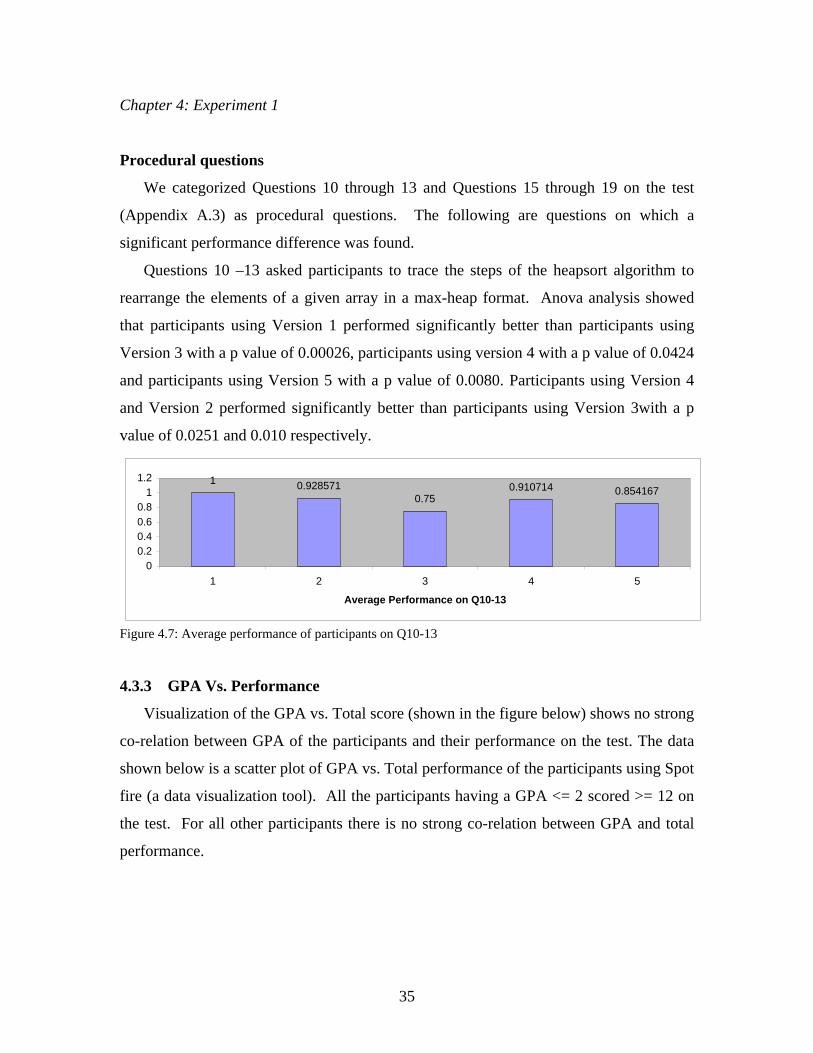
Procedural questions
We categorized Questions 10 through 13 and Questions 15 through 19 on the test
(Appendix A.3) as procedural questions. The following are questions on which a
significant performance difference was found.
Questions 10 –13 asked participants to trace the steps of the heapsort algorithm to
rearrange the elements of a given array in a max-heap format. Anova analysis showed
that participants using Version 1 performed significantly better than participants using
Version 3 with a p value of 0.00026, participants using version 4 with a p value of 0.0424
and participants using Version 5 with a p value of 0.0080. Participants using Version 4
and Version 2 performed significantly better than participants using Version 3with a p
value of 0.0251 and 0.010 respectively.
1 0.9285710.75
0.910714 0.854167
00.20.40.60.8
11.2
1 2 3 4 5
Average Performance on Q10-13
Figure 4.7: Average performance of participants on Q10-13
4.3.3 GPA Vs. Performance
Visualization of the GPA vs. Total score (shown in the figure below) shows no strong
co-relation between GPA of the participants and their performance on the test. The data
shown below is a scatter plot of GPA vs. Total performance of the participants using Spot
fire (a data visualization tool). All the participants having a GPA <= 2 scored >= 12 on
the test. For all other participants there is no strong co-relation between GPA and total
performance.

Chapter 4: Experiment 1
36
Figure 4.8: Scatter Plot of GPA vs. Total Performance of the participants
4.4 Conclusions
The overall performance indicates that participants using Version 1 performed
somewhat better (not significantly) than participants using the other versions. On
performing the individual question analysis, we can infer the reason for this. Participants
using Version 1 significantly outperformed all the other participants (except Version 2)
on procedural questions (Q 10-13). Participants using Version 2 or Version 4 performed
significantly better than those using Version 3 on the procedural questions.
Thus, from the results it can be inferred that a simple visualization that focuses just on
the logical steps of an algorithm and shows its effect on the data would provide better
understanding of the procedural steps of the algorithm to the participants who have no
previous knowledge of the algorithm. The results seem to indicate that a simple
visualization which focuses mainly on the procedural steps of the algorithm may help
participants understand and notice the procedural steps in a better way. Too much
information (like a pseudocode display, an activity guide) may over-whelm participants
and thereby reduce the amount of procedural understanding they may gain from a
visualization. It may also be possible that participants who observe a visualization that
Participants having low GPAs but scoring above average

Chapter 4: Experiment 1
37
focuses on procedural steps of an algorithm may be able to mimic the algorithm steps
better and thereby obtain better results on the procedural questions than participants who
have more amount of detail to work with. Also, working repeatedly with an example data
set as in Version 1 which covers all the important cases in the algorithm may allow
participants to understand the algorithm in a better way. The reason for this may be that
participants who have no previous knowledge of algorithm do not know what would be a
“good” data set to enter and therefore miss some of the important points in the algorithm.
On Question 7 (Appendix A.3), which was a conceptual question, participants using
Version 3 performed significantly better than participants using Version 4 and somewhat
better (p = 0.087) than the participants using Version 2. On Question 8, another
conceptual question (Appendix A.3), participants using Version 5 significantly
outperformed participants using Version 2 or Version 4. Participants using Version 1
outperformed participants using Version 2. Participants using Version 3 outperformed
participants using version 2.
Thus, from the above results it can be inferred that a pseudocode display and an
activity guide or a data example that covers all the important cases may provide better
conceptual understanding of the algorithm. Participants who worked with Version 3 and
Version 5 had a pseudocode of the algorithm displayed to them. Participants who worked
with Version 5 were given an activity guide to work with (Appendix A.2) that made them
analyze and answer questions about the algorithm, provided them with a few data sets to
work with. Participants who had an activity guide usually spent more time with the
visualization as compared to other participants as they had an activity guide to work with.
This may have enabled them to understand the logic of the algorithm in a better way as
compared to Versions 2 and Versions 4 who did not have a pseudocode display.
However the results also inidcate another important point that an example data set may
also help to provide conceptual understanding of the algorithm as the participants using
either the Verison 3 or Version 5 did not perform better than Version 1.

Chapter 4: Experiment 1
38
The question set for Experiment 1 had two questions 9 and 14 (Appendix A.3) that asked
participants pseudocode for the heapsort algorithm. We were surprised by the fact that the
participants who had pseudocode display did not perform better on the pseudocode
questions as compared to the participants who did not have a pseudocode display.

Chapter 5
Experiment 2
This chapter describes the second experiment that we conducted as a part of this
thesis work. Our analysis of the first experiment gave counter-intuitive results (better
performance by the basic version). We then hypothesized that two factors not tested for
were dominating the results: having absolute control on the speed of algorithm execution
and a data example. Thus, we did the second experiment to test this hypothesis.
As in the first experiment, undergraduate students who had prior knowledge about
simple sorting algorithms and knew basic data structures like stacks, queues, single
linked lists, double linked lists, and circular linked lists, participated in this experiment.
Most of these participants had no previous knowledge about the heapsort algorithm or the
heap and tree data structures.
5.1 Procedure
Participants were asked to work with one of four variations of the heapsort algorithm
visualizations. All four variations used the same graphical representation of the algorithm
and the same textual feedback messages used by all the visualizations in Experiment 1.
Besides the algorithm visualization, participants were provided with some background
information on the heapsort algorithm (Appendix A.1).
For each participant, a log file that had a record of the time the participant spent with
the visualization and also number of times that he/she interacted with various interface
was maintained.

Chapter 5: Experiment 2
40
Version 1
Version 1 visualized the heapsort algorithm on a data set that the participants entered.
Participants using this version were not given any example data set to work with. This
version had a “next” button, but no “back” button, no pseudocode panel and no guide.
Figure 5.1: Heapsort Version 1
Version 2
Version 2 extended Version 1 by adding more capabilities to it. The participants
using this version were provided with an example data set and could enter any other data
set to visualize the algorithm. They were also able to revert to a previous step in the
algorithm.

Chapter 5: Experiment 2
41
Figure 5.2: Heapsort Version 2
Version 3
Version 3 extended version 2 by adding more capabilities to it. The participants using
this version were provided with a pseudocode display to show how each individual line
of the heapsort algorithm code affects a given data set. Participants were able to revert to
a previous step in the algorithm. Participants were provided with an example data set
(same as Version 2) to begin the algorithm visualization. They could also enter any other
data set. They were also provided with a paper reference material (Appendix A.2) to
make them explore the algorithm in a more detailed way.

Chapter 5: Experiment 2
42
Figure 5.3: Heapsort Version 3
Version 4
Figure 5.4: Version 4 (Animation)
Unlike all the other visualizations created as a part of this thesis work, Version 4
animated the heapsort algorithm on a data set entered by the students. The participants
using this version could control the speed of animation, but did not have a ‘Next’ button.
Also as in Version 1 no example data set was provided to students.

Chapter 5: Experiment 2
43
Features provided in each of the above four versions can be summarized as in the
following table.
Version 1 Version 2 Version 3 Version 4
Input Next button
Input Example Next button Back button
Input Example Guide Pseudocode Next button Back button
Input Animation (No next button)
Table 5.1: Feature list for all versions.
When the participants thought that they were sufficiently familiar with the algorithm,
they were asked to answer questions (Appendix A.4) about the heapsort algorithm.
Participants performance on the test would determine the effectiveness of each Version.
Question set
The results of Experiment 1 seem to indicate that participants who had a simple
visualization that focused mainly on the logical steps of the algorithm performed better
on procedural questions as compared to participants who had a pseudocode display or
pseudocode display and activity guide. The results seem to suggest that participants who
had more amount of detail presented to them (e.g. pseudocode display and activity guide)
tend to perform worse on the procedural questions. To further analyse the results obtained
from Experiment 1 we included more procedural questions in the question set for
Experiment 2 as compared to the question set for Experiment 1.
The question set for Experiment 2 had a total of 24 questions (Appendix A.4). We
divided the questions into two groups: Conceptual and Procedural questions. Questions 1
through 5 were grouped as conceptual questions whereas the remaining questions were
grouped as procedural questions. Questions 6–8 asked participants to rearrange a given
array of 3 numbers in max-heap format. Questions 9-13 asked participants to rearrange an
array of 4 numbers in a max-heap format. Questions 14-16 asked participants to sort an

Chapter 5: Experiment 2
44
array of 3 numbers after the first max-heap has been created. Questions 17-24 asked
participants to sort an array of 4 numbers after the first max-heap has been created.
5.2 Hypothesis
The results from the experiment 1 (Chapter 4) indicated that participants who used a
minimal algorithm visualization (without many features) that focused mainly on the
logical steps of the algorithm performed better on procedural questions. The results also
indicated that a good data example and the pseudocode of an algorithm help in increasing
students’ conceptual understanding of an algorithm. The results seem to indicate that
providing a good example can prove to be most helpful to increase the pedagogical
effectiveness of an algorithm visualization.
To analyze the importance of a good data set (a data set that covers all the important
cases in an algorithm) for conceptual understanding of the algorithm, participants were
asked to study the heapsort algorithm with Version 1 and Version 2. Both the versions
were almost identical except that participants using Version 2 were provided with a data
example and could revert to a previous step in the algorithm. This would allow us to
measure the difference in conceptual understanding of the two groups and determine if a
good data set could increase the participants conceptual understanding of an algorithm.
Version 3 used a pseudocode display, a data set example, and a guide that made students
explore the algorithm in detail. By this, we wanted to see if providing all these features
could further increase conceptual understanding of the algorithm.
If Version 3 outperformed all the other versions on the conceptual questions, than
based on the first and second experiment we would be able to conclude that providing
additional features (like pseudocode and an activity guide) could increase students
conceptual understanding of an unfamiliar algorithm. If there is a significant difference
between performance of the students using Version 1 and Version 2 or Version 1 and
Version 3 but no significant difference between the performance of students using
Version 2 and Version 3, then we would conclude that providing a good data example
can prove to be most helfpul in understanding the concept of an unfamiliar algorithm.

Chapter 5: Experiment 2
45
Results from Experiment 1 indicated that students who used minimal algorithm
visualization (without many features) performed well on procedural questions. Also in
Experiment 1 students who had a pseudocode display performed significantly worse on
these questions. We should be able to analyze by comparing the performance of the
students on questions 6-24 (Appendix A.4) using Version 1, Version 2 and Version 3,
whether providing more features could result in reduced procedural understanding of the
algorithm. Through this analysis we should also be able to understand the importance of
providing a data set to understand the procedural steps of an algorithm.
We also believed that allowing students to control the speed of algorithm execution
would prove more helpful to understand an algorithm than showing an animation that
does not provide absolute control on the algorithm execution. If our hypothesis was true
then the students using Version 1 (Input) should perform better than students using
Version 4 (animation).
It is commonly assumed that the more time students spend with an algorithm
visualization, the better understanding they have from the visualization. For the first
experiment we did not measure the learning time (the amount of time students with the
algorithm visualization) but for the second experiment we kept track of the learning time
to know if there is any significant relation between the time students spend with the
algorithm visualization and the score that they got on the test. Also, while creating the
algorithm visualizations, many authors assume that it would help students if they could
revert to a previous step in the algorithm visualization. We wanted to see if there was any
specific relation between the usage of the history or the ‘back button’ and the scores
students obtained on the test.
5.3 Results
5.3.1 Total Performance
44 Students, 11 for each version, participated in the experiment. The average GPAs of
the participants of each group were almost similar. Anova analysis on the GPAs did not
show any significant difference. The following is a bar chart showing average

Chapter 5: Experiment 2
46
performance of each version. The anova analysis for the total performance and GPAs of
students is included in Appendix A.6.
16.6363618.81818
10.18182
22.27273
0
5
10
15
20
25
1 2 3 4
Average Performance
Figure 5.5: Average performance of participants of each version.
The following is the summary of average performance of the participants
Version 1 (Input Only)
Significantly worse than Version 2 (p=0.008)
Non-significantly worse than Version 3 (p=0. 35)
Significantly better than Version 4 (p = 0.03)
Version 2 (I +H+Ex)
Significantly better than Version 1 (p=0.008)
Non-significantly better than Version 3 (p=0.10)
Significantly better than version 4 (p=0.0001)
Version 3 (P+I+H+Ex+G)
Non-significantly better than Version 1 (p=0. 35)
Non-significantly worse than Version 2 (p=0.107)
Significantly better than Version 4 (p=0.006)
Version 4 (Animation)
Significantly worse than Version 1 (p = 0.029)
Significantly worse than Version 2 (p=0.0001)
Significantly worse than Version 3 (p=0.006)
Table 5.2: Summary of total performance.
The following is the partial ordering on the results for each version. The circular
nodes represent each version (V1 = Version 1, V2 = Version 2, V3 = Version 3 and V4 =
Version 4). The arrows are from the nodes (i.e. Version) that performed poor towards the
nodes (i.e. Version) that had better performance. The dotted arrows indicate non-
significant results where as a bold arrow indicates a significant performance difference.

Chapter 5: Experiment 2
47
Figure 5.6: Partial ordering on total performance of participants of each version.
As shown in the above table and partial order figure, participants who used Version 4
performed significantly worse than other participants. From this we can conclude that the
providing an ability to control the pace of the visualization is very important. Participants
using Version 2 performed significantly better than the participants using Version 1.
From this we can conclude that providing a data set that covers all the important cases in
an algorithm can prove to be pedagogically very effective.
5.3.2 Individual Question analysis
Anova analysis for the Individual questions are included in Appendix A.6.
Conceptual Questions
Questions 1-5 (AppendixA.4): Participants using Versions 2 and 3 performed slightly
better than those using Version 1 and Version 4 as shown by the average scores in the
following bar char. However, on performing Anova analysis there was no significant
performance difference.
V1
V3
V4
V2

Chapter 5: Experiment 2
48
3.636364
4.636364 4.6363644.272727
0
1
2
3
4
5
1 2 3 4
Average Performance on Conceptual Questions
Figure 5.7 Average Performance on Conceptual Questions
Procedural questions
Questions 6 – 24 on the test (Appendix A.4) were categorized as procedural
questions. On perfoming Anova analysis on performance on these questions we
discovered that participants using Version 2 performed significantly better than Version 1
(p=0.01479). Participants using Version 4 performed significantly worse than
participants using all other versions p= 0.0139 as compared to Version 1, p= 0.000086 as
compared to Version 2 and p= 0.0057 as compared to Version 3.
12.90909091
17.63636364
14.18181818
5.909090909
0
5
10
15
20
1 2 3 4
Average Performance on Procedural Questions Q6-24
Figure 5.8 Average Performance on Procedural Questions
The following is a summary of the results on Anova analysis for individual
procedural questions.

Chapter 5: Experiment 2
49
Questions 6-8 (Appendix A.4) asked students to trace the steps of the heapsort
algorithm to rearrange a given array having 3 numbers in max-heap format. Participants
using Version 1 performed significantly (p=0.02678) better than Version 4.
3
2.454545 2.272727
1.727273
00.5
11.5
22.5
33.5
1 2 3 4
Average Performance on Q6-8
Figure 5.9: Average performance of the participants on Q 6-8.
Questions 9-13 (Appendix A.4) asked students to trace the steps of the heapsort
algorithm to re-arrange a given array of 4 numbers in a max-heap format. Participants
using Version 2 performed significantly better than participants using Version 1
(p=0.009). Participants using Version 2 and Version 3 performed significantly better than
participants using Version 4 with p=0.0006 and p=0.008 respectively.
2.727273
5 4.545455
2
0
2
4
6
1 2 3 4
Average Performance on Q9-13
Figure 5.10: Average performance of the participants on Q 9-13.
Questions 14 – 16 (Appendix A.4) asked students to trace steps of the heapsort
algorithm to sort a given array of 3 elements after the first max-heap has been created.
The participants using Version 4 performed worse than all other versions with p=0.03,
p=4.030E-06, and p=0.008 as compared to Version 1, Version 2 and Version 3

Chapter 5: Experiment 2
50
respectively. Participants using Version 2 also performed significantly better than
participants using Version 1 with p=0.02.
1.818182
2.909091
2.181818
0.545455
00.5
11.5
22.5
33.5
1 2 3 4
Average Performance on Q14-16
Figure 5.11: Average Performance of participants on Q14-16.
Questions 17- 24 (Appendix A.4) asked participants to trace steps of the heapsort
algorithm to sort elements of a given array of 4 numbers after the first max-heap has been
created. Participants using Version 4 performed significantly worse than participants
using than participants using Version 1with p=0.016 and those using Version 2 with
p=0.0001. Participants using Version 2 performed marginally better than participants
using Version 3 (p=0.059).
5.363636
7.272727
4.363636
1.454545
0
2
4
6
8
1 2 3 4
Average Performance on Q17-24
Figure 5.12: Average Performance on participants on Q17-24.
The above results on the pseudocode questions can be summarized as in the following
table.

Chapter 5: Experiment 2
51
Questions 6 -8 Version 1 performed better than version 4. Questions 9-13 Participants
using Version 2 performed significantly better (p = 0.009) than those using Version 1
Participants using Version 2 performed significantly better (p= 0.0006) than those using Version 4
Participants using Version 3 performed significantly better than those using Version 4 (p=0.008)
Participants using Version 3
performed marginally better than those using Version 1 (p=0.059).
Questions 14-16 Participants using Version 1 performed significantly better (p= 0.03) than participants using Version 4
Participants using Version 2 performed significantly better (p=0.020) than participants using Version 1
Participants using Version 2 performed significantly better (p=4.030E-06) than participants using Version 4.
Participants using Version 3 performed significantly better (p=0.008) than those using Version 4.
Questions 17-24 Participants using Version 1 performed significantly (p= 0.016) better than the participants using Version 4
Participants using Version 2 performed significantly better than the participants using Version 4 (p= 0.0001
Participants using Version 2 performed marginally better than those using Version 3 (p= 0.0592).
Participants using Version 3 performed marginally better than those using Version 4 (p= 0.0828).
Table 5.3: summary of performance on individual questions.
5.3.3 Performance vs. Learning Time
The following is a scatter plot of Learning Time Vs. Average Performance. As shown
in the below scatter plot, more time spent with the visualization does not imply that
students would have better understanding of the algorithm. Participants using Version 3
spent about 41.73 minutes studying the applet and working with the guide, however this
did not result in better scores than the participants using Version 2 who spent only an
average of 18.73 minutes with the visualization.
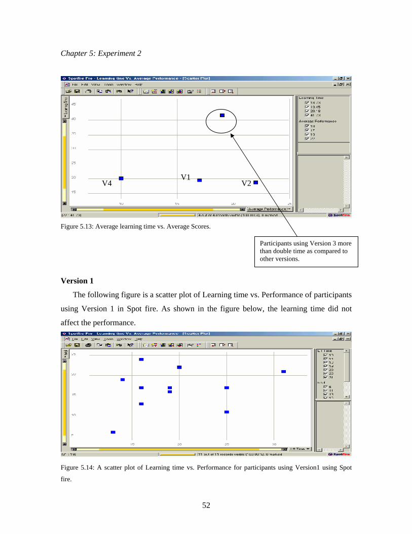
Chapter 5: Experiment 2
52
Figure 5.13: Average learning time vs. Average Scores.
Version 1
The following figure is a scatter plot of Learning time vs. Performance of participants
using Version 1 in Spot fire. As shown in the figure below, the learning time did not
affect the performance.
Figure 5.14: A scatter plot of Learning time vs. Performance for participants using Version1 using Spot
fire.
Participants using Version 3 more than double time as compared to other versions.
V2 V1
V4

Chapter 5: Experiment 2
53
Version 2
As shown in the figure below, the learning time did not have any significant effect on
performance of participants using Version 2. The following is a scatter plot of Learning
time vs. Performance of participants using Version 2 in Spot fire.
Figure 5.15: A scatter plot of Learning time vs. Performance for participants using Version 2 using Spot
fire.
Version 3
Like the previous two versions, there was no relation between learning time and
performance of the participants.

Chapter 5: Experiment 2
54
Figure 5.16: A scatter plot of Learning time vs. Performance for participants using Version 3 using Spot
fire.
Version 4
Again there was no correlation between learning time and performance for
participants using Version 4.
Figure 5.17: A scatter plot of Learning time vs. Performance for participants using Version 4 using Spot
fire.
5.3.4 GPA vs. Performance
The following figure shows a scatter plot of GPA vs. Total performance of
participants. No strong correlation is seen between GPA of participants and their

Chapter 5: Experiment 2
55
performance. However, it is interesting to note that all the 3 participants having low GPA
(<= 2.25) performed well on the test.
Figure 5.18: Scatter plot of GPA vs. Total Score using Spot fire.
5.3.5 Example Usage
Both Version 2 and Version 3 provided a data set example to the participants. The
following figures are the visualizations of number of times the participants worked with
the example and their scores.
Version 2
The below visualization suggests that the participants who worked more than twice
with the data set example had a full score on the test as compared to the participants who
worked just once with it. Thus, the example data set may have helped the participants.
The data in the figure below is sorted on example usage.
All the participants having GPA <= 2.25 performed well.

Chapter 5: Experiment 2
56
Figure 5.19: Scatter plot of example usage vs. Total Score for Version 2.
Version 3
As shown in the visualization, there was no relation between the number of times the
participants studied the example and the total score they got on the test.
Figure 5.20: Scatter plot of example usage vs. Total Score for Version 3.
Participants who worked with example atleast 3 times could answer all the questions on the test correctly.

Chapter 5: Experiment 2
57
On average the participants using Version 3 (average = 3.3636) studied the example
more number of times than the participants using Version 2 (average = 2.3636).
5.3.6 History (Back Button) Usage
Participants using Version 2 and Version 3 were provided with a Back button so that
they could revert to a previous step in the algorithm and reuse it again.
Version 2
The participants using Version 2 did not use this button much. Most of the
participants (6/11) did not use it at all. As shown in the figure below there is no
correlation visible between the usage of back button and total scores on the test.
Figure 5.21: Scatter plot of Back button usage vs. Total Score for Version 2.
6 out of 11 participants did not use back button at all.

Chapter 5: Experiment 2
58
Version 3
Participants using Version 3 used the back button more than the participants using
Version 2. As shown in the figure below there was no significant relation between the
back button usage and the total scores. On average participants using Version 3 used back
button more than participants using Version 2.
Figure 5.22: Scatter plot of Back button usage vs. Total Score for Version 3.
5.3.7 Subjective Satisfaction
The last question on the test (Appendix A.4) asked students to rate the visualization
that they worked on between a scale of 1-5. Anova analysis indicated that Version 2 had
a significantly higher rating as compared to Version 4 with p=0.038687. The following is
a bar chart showing average subject satisfaction for each group.
3.8181
4.3636
4
3.5
3
3.5
4
4.5
1 2 3 4
Subjective Satisfaction
Figure 5.23: Average subjective satisfaction for each version.

Chapter 5: Experiment 2
59
5.4 Conclusions
Participants using Version 1, Version 2 and Version 3 significantly outperformed
participants using Version 4. Versions 1 and 4 had all features but the control of
algorithm execution in common.
Thus, providing students an absolute control on the speed of algorithm execution can
prove to be most helpful. Based on the results obtained in Experiment 2 we recommend
that “animations” with speed control be replaced with a ‘Next’ button for controlling
progress of an algorithm.
On procedural questions, participants using Version 1 performed significantly better
than participants using Version 4 and participants using Version 2 performed
significantly better than participants using Version 1. The only difference between
Version1 and Version 4 was that Version 1 had a ‘Next’ button which allowed the users
Thus, providing a good data example and having an absolute control on the algorithm
execution would be very helpful in procedural understanding of the algorithm.
Version 2 and Version 3 had every feature other than pseudocode display and study
Guide (Appendix A.2) in common. It seems from the results of Experiment 2 that having
too many features may reduce students’ procedural understanding of the algorithm (On
average participants using Version 2 performed better on procedural questions as
compared to participants using Version 3 but there was no significant performance
difference). The learning time vs. performance analysis showed that a larger learning
time (at least when that time is spent observing pseudocode and working with guide) does
not mean that participants understood the algorithm better. The participants using Version
3 spent almost double amount of time with the visualization as compared to the
participants using Version 2. This shows that having the right set of features would
improve learning in less time, also using more features could result in increase in the
learning time without any pedagogical benefit.
There was no significant performance difference on the conceptual questions on the
test for Experiment 2 between participants using various versions. There was no
performance difference between participants using Version 2 and Version 3 on

Chapter 5: Experiment 2
60
conceptual questions (Q 1-5, Appendix A.4). Results from Experiment 1 indicated that
additional features like pseudocode and guide might prove to be helpful in increasing
conceptual understanding of the algorithm. Both Version 2 and Version 3 provided
participants with an example data set to work with. Besides example data set, participants
using Version 3 also had a pseudocode display and a guide to work with, which the
participants using Version 2 did not have. However, there was no performance difference
on the conceptual questions between Version 2 and Version 3. Thus, having a good
example data set that covers all the important cases in the algorithm may be sufficient in
providing conceptual understanding of the algorithm. Also, features like pseudocode
display and an activity guide increase learning time significantly.
From the experiments 1 and 2, we can conclude that a minimal visualization that
focuses on the logical steps of the algorithm and allows students to have absolute control
on the speed of algorithm execution is most helpful for procedural understanding of the
algorithm. Also, providing an algorithm that has too many features may confuse the
users.
GPA vs. performance analysis on the tests for both Experiment 1 and Experiment 2
indicated that students having an extremely low GPA often performed well using the
visualization. This indicates that if visualizations are used for teaching algorithms in class
these students may benefit. However, we did not conduct an experiment explicitly to test
this hypothesis.

Chapter 6
Algorithm Visualizations
This chapter describes several algorithm visualizations that were created early in this
thesis work, before we decided to focus on studying the key feature set.
6.1 Graph Traversals
The graph traversal applet visualizes Breadth First Search (BFS) and Depth First
Search (DFS) algorithms and illustrates step-by-step, how graphs are traversed in each
case.
Figure 6.1: The initial interface when the user starts the applet.
When a user starts the visualization the text display as shown above instructs him/her
to ‘Input’ a file that has the specification for the graph on which the algorithm will be
executed. Clicking the ‘Input’ button pops up a dialog box to select the file.

Chapter 6: Algorithm Visualizations
62
Figure 6.2: Dialog box to select the file.
The applet reads the selected file and displays the graph as shown in the figure below.
Figure 6.3: The graph display. The text field displays the textual feedback.
The graph display, as shown above, is divided into two parts. The top part shows the
graph visualization and the bottom part shows the visualization of a queue or a stack
depending on the algorithm selected. The queue/stack is initially empty.

Chapter 6: Algorithm Visualizations
63
The default algorithm selected by the system is BFS. Users can change the algorithm
using the provided Combo box. To select the starting node a user will click on one of
graph nodes. The node that has been selected is shown pink in color as shown in the
figure below. The user will step through the algorithm by pressing the ‘Next’ button
repeatedly.
Figure 6.4: The starting node is highlighted in pink.
Different color combinations have been used to show different stages of the graph
traversal (shown in the figure below). An un-traversed graph is shown in gray. The
starting node is shown in dark pink. The current active node is shown in dark green. The
nodes that are in Queue/Stack are shown in light green color and are also displayed in the
queue/stack box at the bottom of the screen. The current active edge being traversed from
the current active node to the other node is shown in dark green. The edges that are in the
BFS/DFS tree are shown in dark pink. The edges that have been traversed but do not
belong to the tree are shown in light pink color. The un-traversed nodes and edges are left
in gray. Each step of the algorithm is also explained using text messages in the text field
on the right side of the screen.

Chapter 6: Algorithm Visualizations
64
Figure 6.5: Different color combinations used in the visualization as explained in the paragraph below.
Users can also refer to the help manual if there is any confusion about the interface or the
graphical display. The help manual is displayed when the help button is clicked.
Figure 6.6: Help Manual.

Chapter 6: Algorithm Visualizations
65
As shown in the figure below, once the graph traversal is complete, nodes that were
visited are shown in pink and the starting node in dark pink. All the traversed edges are in
pink with the BFS/DFS tree highlighted.
Figure 6.7: A traversed graph.
The unvisited nodes and edges in the graph are left in gray as shown in the figure below.
Figure 6.8: A traversed graph.

Chapter 6: Algorithm Visualizations
66
Format for Graph Specification
The applet reads a graph from a file with the following format
1. All the statements starting with ‘#’are treated as comments and ignored.
2. Specify number of nodes in digits like 1, 2 etc.
3. Optionally, X and Y co-ordinates are specified to position the nodes on the display.
The graph display is divided into a 1000 X 1000 co-ordinate system. If the co-
ordinates are not specified, the graph nodes are displayed in a circle.
4. Specify the graph type by using the characters ‘U’ (Undirected) or ’D’ (Directed).
5. Specify the number of edges.
6. In a separate line, for each edge, specify the starting and the ending node.
A file format example is shown below
# You can include more comments using the ‘#’ sign
4 # Number of vertices the co-ordinates for each vertex are below
10 40 # The X and Y co-ordinates
700 10
200 250
400 500
U #Undirected graph
5 # Number of edges
0 1 # the starting and the ending node for each edge
0 2
2 1
2 3
3 1

Chapter 6: Algorithm Visualizations
67
6.2 Skip Lists
The Skip List applet visualizes the Skip List data structure. The applet illustrates step-
by-step insertion and search of an element in a Skip List.
When a user starts the visualization the text display, as shown below, instructs the
user to enter an element in the text field. When the user enters an element the Skip List is
displayed as shown below.
Figure 6.9: Initial Skip list.
The Input/Search button is used to specify the operation to be performed on the element
that is entered. The users will trace the insertion or search operation by pressing the Next
button. As shown in the figure below the pointers are highlighted using green color. The
position to insert the element is displayed using a red arrow.

Chapter 6: Algorithm Visualizations
68
Figure 6.10: The current pointer is highlighted. The red arrow shows the position to insert the element
For the search operation the element, if found in the list, is highlighted using pink color.
If the element that is being searched is not present in the Skip List then a message “The
number was not found” is displayed as shown in the figure below.
Figure 6.11: The element is found in the list.

Chapter 6: Algorithm Visualizations
69
6.3 Memory Management (Buffer Pool Applet)
The total number of pages that can be stored in the buffer pool or main memory is
quite less than the total number of pages on the secondary storage device. As long as
there is an unused buffer available in the buffer pool, new information can be read in
from the disk as demanded but as an application continues to read new information, from
the secondary storage device, eventually all the buffers from the buffer pool will become
full. Once this happens, some decision has to be made about what information in the
buffer pool will be removed to make room for the newly requested information. The goal
is to select the page that has the information that is least likely to be requested again.
Since the buffer pool cannot know for certain what the pattern of future requests will be,
a decision based on some heuristic, or best guess, is made. This applet presents
visualizations of the following heuristics.
First In First Out (FIFO): This approach stores the buffers in a queue. When the
buffer pool is full the buffer at the front of queue is removed and the new buffer is stored
at the end of the queue.
Least Recently Used (LRU): LRU simply keeps the buffers in a linked list.
Whenever information in a buffer is accessed, this buffer is brought to the front of the
list. When new information is to be read, the buffer at the end of the list is taken off and
the new buffer is inserted in the front of the list.
Least Frequently Used (LFU): LFU tracks the number of accesses to the each buffer
in the buffer pool. When a buffer has to be replaced, the one with the least number of
accesses is removed.
When a user starts the visualization the text display, as shown below, instructs the
user to select one of the buffer management algorithms that the user wants to visualize.

Chapter 6: Algorithm Visualizations
70
Figure 6.12: The starting interface of the system.
Users need to enter the page number to be inserted in the main memory. Memory
updates depend on the algorithm that is selected. Users will step through the algorithm by
pressing the ‘Next’ button repeatedly.
Figure 6.13: The pages that have been inserted in the main memory.
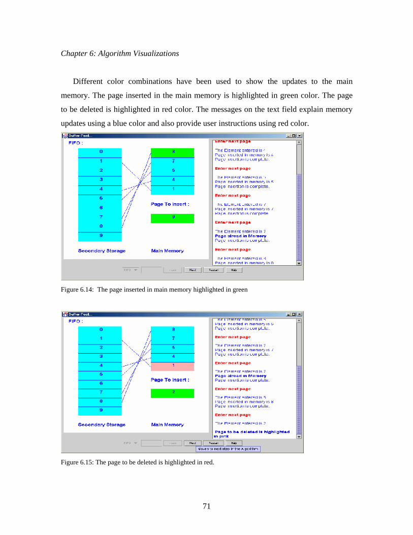
Chapter 6: Algorithm Visualizations
71
Different color combinations have been used to show the updates to the main
memory. The page inserted in the main memory is highlighted in green color. The page
to be deleted is highlighted in red color. The messages on the text field explain memory
updates using a blue color and also provide user instructions using red color.
Figure 6.14: The page inserted in main memory highlighted in green
Figure 6.15: The page to be deleted is highlighted in red.

Chapter 6: Algorithm Visualizations
72
If a user chooses to visualize ‘Least Frequently Used’ memory management algorithm,
then the number of accesses to the page are also displayed.
Figure 6.16: The number of disk accesses in case of LFU algorithm.
6.4 Hash Algorithms
In a hash algorithm, the address where the data is stored is calculated and stored in a table
along with a key value. The table that stores the addresses of the data items along with
their key values is called the hash table. The function that calculates the address where
the data is to be stored in the data structure and maps them to key values is called a hash
function and the process is called hashing. The hashing functions that have been
visualized in this applet are.
1) Mod Function: (Take the remainder (Modulus) of the number and table size)
2) Add Digits: (Add the digits of the number and take modulus with the table size)
3) Reverse Digits: (Reverse the digits of the number and take modulus with the table
size)
4) Mid-Square: (Take the middle bits of the square of the number entered, and perform
modulus operation on the value of the middle bits with the table size)

Chapter 6: Algorithm Visualizations
73
Linear probe collision resolution policy has been used for all the hash functions.
Figure 6.17: the various hash function available to the users.
When a user starts the visualization, the text display as shown above, instructs the
user to select the hash function. Then the user selects the size of the table.
Figure 6.18: The hash table.

Chapter 6: Algorithm Visualizations
74
The hash table is displayed when the user selects the table size. The user then needs to
input a number, using the text input field, to enter into the table. The user will compute
the hash key by pressing the hash key button. As shown in the figure below, feedback is
provided on the display about the hash key and the function used to calculate it.
Figure 6.19: Hash value and the hash function used.
The user then steps through the algorithm using the next button. The slots in the table are
highlighted depending on the values that are generated using the hash function as shown
in the figure below.

Chapter 6: Algorithm Visualizations
75
Figure 6.20: The position calculated by the hash value is highlighted.
If a collision resolution policy is used to determine an empty space to store the new data
item, the user is given feedback about how the table position was recalculated using the
collision resolution.
Figure 6.21: The collision resolution policy.

Chapter 6: Algorithm Visualizations
76
6.5 Collision Resolution Applet:
Typically for hashing algorithms, the range of hash key is comparatively larger than
the number of slots in the hash table and so it is probable that multiple key values would
be mapped to the same slot in the hash table. Given a hash function H and two key values
K1 and K2, if H(K1) = H(K2) = j, where j = slot in the table, then we say that keys K1 and
K2 have a collision at slot j under the hash function H. Thus, to search a record with the
key value K using hash function H, we go through the following two steps.
a) Compute the table location H(K).
b) Starting with the table slot H(K), locate the record containing key K (if there is a
collision) using a collision resolution policy.
The collision resolution functions visualized in this applet are as follows:
1. Linear Probing
2. Linear probing with steps
3. Quadratic probing.
4. Double hashing
5. Pseudorandom probing
A common hash function which performs a modulus operation on the number entered
and the table size and uses the remainder as the hash value is used for all the collision
resolution mechanisms.

Chapter 6: Algorithm Visualizations
77
Figure 6.22: The user needs to select the table size first.
When a user starts the visualization, the text display as shown above, instructs the
user to select the table size to be implemented using the combo box. The collision
resolution policy to be visualized can be selected using the other combo-box.
Figure 6.23: Hash Table. The collision resolution policy to be implemented is also displayed.

Chapter 6: Algorithm Visualizations
78
The user after entering a number can compute the hash key by pressing the ‘hashkey’
button. The computed hash key and the function used are displayed on the display area.
Figure 6.24: The hashkey is displayed on the display area.
The user will step through the algorithm using the next button. The slots in the table
corresponding to the calculated hash key are highlighted as shown in the figure below.

Chapter 6: Algorithm Visualizations
79
Figure 6.25: The columns are highlighted in the table.
If the slot computed by the hash function is already occupied, the new position and the
collision function used are displayed as shown below.
Figure 6.26: The collision resolution policy displayed on the display area.

Chapter 7
Conclusions and Future Work
7.1 Conclusions
We started our work by reviewing some of the well-known algorithm visualizations
that have been developed over many years. The primary focus of this study was to know
the system capabilities or features provided to users for effective learning. We also
reviewed the current research on algorithm visualizations effectiveness to understand
features in these systems that have proved to have positive learning effect on users
(Chapter 2). Based on our studies, we hypothesized that certain features when
incorporated into an algorithm visualization would make it more effective for users. We
then proceeded to compile a list of candidate features that we believed might increase the
pedagogical effectiveness of an algorithm visualization (Chapter 3). To measure the
effect of each individual feature and identify the most important features from this list,
we conducted two experiments using a variety of heapsort algorithm visualizations.
The following is a list of the key findings from our experiments.
• When a user can control the pace of algorithm visualization, it significantly increases
the pedagogical value of the visualization.
• Providing students with an example data set that covers all the cases in an algorithm
significantly increases the pedagogical value of the visualization.
• Participants having pseudocode display and an activity guide spend substantially
more time with the visualization as compared to simple visualizations that do not
have there features. Also these participants do not perform better on procedural
questions as compared to those participants who do not have these features.

Chapter 7: Conclusions and Future Work
81
Earlier in our work we had developed a set of features that that we believed should be
taken into account while designing an algorithm visualization to increase its pedagogical
value. This feature set is presented in Chapter 3.
The results of our experiments suggest that we were correct in some of our
assumptions and that certain features do significantly increase the pedagogical
effectiveness of an algorithm visualization. From the features that we had mentioned
earlier, we found that being able to control all the steps of the algorithm and providing a
data example that covers all the significant cases of the algorithm can significantly
increase the pedagogical value of an algorithm visualization. But the experiments also
indicated that we were wrong about certain features. Features like pseudocode display,
an activity guide and using a history mechanism to revert to a previous step in the
algorithm did not prove to have significant pedagogical effectiveness. Also, the results
seem to indicate that providing users with a data input ability to enter their data sets need
not result in a significant pedagogical value. There are other features a visualization
should provide; appropriate feedback messages, if applicable a visualization should show
both the physical view and the logical view of the data structure that the algorithm
assumes, if a visualization uses multiple windows it is necessary to provide an effective
window management, a visualization should show state changes in the algorithm and the
updates to a data set or a particular data structure clearly) that we have not tested and
cannot guarantee that they would have a significant pedagogical value.
7.2 Future Work
On performing the analysis of total scores in the experiment and GPA (Grade Point
Average) of participants, we noticed that many students having low GPAs (< 2.0/4.0)
performed really well on the test as compared to the students who have high GPAs. As
future work, it would be interesting to know if there is any correlation between GPA and
participants performance in the experiments. If participants who have low GPA
consistently perform better than expected, it means that visualizations may help to
explain the concepts and working of an algorithm for these students.

Chapter 7: Conclusions and Future Work
82
As mentioned, our work focused mainly on finding key features that would make an
algorithm visualization pedagogically more effective. However, we did not measure the
advantage of using an algorithm visualization as compared to the course textbook. We do
not know if an algorithm visualization that was mostly similar to Version 2 of
Experiment 2 would provide more pedagogical benefit than the normal course textbook.
It would also be interesting to know if there is any advantage to using the algorithm
visualization together with the course textbook.
For our experiments we focused on 3 features (data example, pseudocode, user
control) from the list of features that we created. From the results of Experiment 1 and
Experiment 2 we can conclude that providing users with a data example and user control
over the speed of algorithm execution can significantly increase the pedagogical
effectiveness of an algorithm. It would be interesting to know if other features from the
feature list would have any effect in increasing the pedagogical value of the algorithm
visualizations.
The activity guide for our experiments was a paper-based question set. Many systems
(like HalVis) have an activity guide or some comparative mechanism built in the
algorithm visualization. In these systems, students are prompted for answers while they
are working with the visualization. It would be interesting to know if a paper guide can
be substituted with a guide that is built in to the system or whether a guide that is built in
to the visualization increases its pedagogical value more as compared to a paper guide.
Our experiments concentrated on the heapsort algorithm, which is a relatively simple
algorithm. For the future work, it would interesting to know if the results obtained for this
algorithm would also remain true for more complex algorithms.
We tested for short-term gain of knowledge. Participants worked with the
visualization and answered questions immediately after working with it. It would be
interesting to know if algorithm visualizations could help in a long-term gain of
knowledge. Is there any advantage to using algorithm visualizations to teach an
algorithm to students? Do the students who are taught algorithms in the class using
visualizations perform better towards the end of the semester as compared to students

Chapter 7: Conclusions and Future Work
83
who are taught by conventional teaching methods? It would also be interesting to know if
students who have algorithm visualizations to work with for their homework assignments
show increased learning as compared to students who do not use visualizations for this
purpose.

Bibliography
1. Baker, J. E., Cruz, I. F., Liotta, G., and Tamassia R., A New Model for Algorithm Animation over WWW. ACM Computing Surveys, 27(4): 568-572, 1995.
2. Baker, J. E., Cruz, I. F., Liotta, G., and Tamassia R., Animating geometric algorithms over the Web. In Proc. 12th Annu. ACM Sympos. Comput. Geom., pages C3-C4, 1996.
3. Bergin, J., Brodlie, K., Goldweber, M., Jimenez-Peris, R., Khuri, S., Martinez, M., McNally, M., Naps, T., Rodger, S., and Wilson, J. An Overview of Visualization: Its Use and Design. Report of the Working Group on Visualization. Proceedings of the Integrating Technology into Computer Science Education Conference, 1996. Also published in the SIGCSE Bulletin, volume 28, 1996.
4. Boroni, C.M., Eneboe, T.J., Goosey, F.W., and Ross, J.A., Dancing with DynaLab: Endearing the Science of Computing to the Students. Proceedings of the 27th SIGCSE Technical Symposium on Computer Science Education (SIGCSE Bulletin), volume 28, number 1, pages 135-139, March1996.
5. Brown, M. H., Perspectives on Algorithm Animation, CHI'88 Human Factors in Computing Systems, Washington, DC, USA, pp. 33-38, 1988.
6. Brown, M.H., Exploring Algorithms Using Balsa-II. IEEE Computer 21(5): 14-36 1988.
7. Brown M.H., and Hersberger, J., Color and sound in algorithm animation. IEEE Computer, 25(12):52-63, 1991.
8. Brown, M.H., Sedgewick, R., Techniques for Algorithm Animation. IEEE Software 2(1): 28-39, 1985.
9. Brown M.H., and Sedgewick R., Techniques for Software Animation. IEEE Software, 2(1):28-39, 1985.
10. Cox, K.C., and Roman, G.C., An evaluation of PAVANE visualization system, Department of Computer Science, Washington University at St. Louis, St. Louis, MO, Technical Report, WUCS-94-09, April 1994.
11. Crosby M. E., and Stelovsky J., From multimedia instruction to multimedia evaluation. Journal of Educational Multimedia and Hypermedia 4, 147-162, 1995.
12. Gloor, P., AACE: Algorithm animation for computer science education, Proceedings of the 1992 IEEE International Workshop on Visual Languages, Seattle, Washington, pp. 25-31. 99, September 1992.
13. Gurka J.S., Pedagogic aspects of Algorithm Animation. Unpublished Ph.D. dissertation 1996, Department of Computer Science, Univerity of Colorado.
14. Gurka J.S., and Wayne C., Testing Effectiveness of Algorithm Animation, Proceedings of the 1996 IEEE Symposium on Visual Languages, pages 182-189, Boulder, CO, September 1996.

Bibliography
85
15. Hansen, S., Narayanan, N. H., Schrimpsher, D. and Hegarty, M. Empirical studies of
animation-embedded hypermedia algorithm visualizations, CSE98-06, Dept. of Computer Science & Software Engineering Technical Report Series, Auburn University, Auburn, AL 36849-5347, 44 pages. Journal of Visual Languages and Computing 1998.
16. Hansen, S. R., Narayanan, N. H. and Schrimpsher, D., Helping learners visualize and comprehend algorithms. Interactive Multimedia Electronic Journal of Computer-Enhanced Learning, 2(1), Association for the Advancement of Computing in Education, May 2000.
17. Hansen, S. R., and Narayanan, N. H., On the role of animated analogies in algorithm visualizations. Proceedings of the Fourth International Conference of The Learning Sciences, Lawrence Erlbaum Associates, pp. 205-211, 2000.
18. Hartley, Stephen J., Animating Operating Systems Algorithms with XTANGO, Proceedings of the 1994 ACM SIGCSE Technical Symposium, Phoenix, AZ, pp. 344—348, Mar. 1994.
19. Hundhausen, C.D. & Douglas, S.A., Using Visualizations to Learn Algorithms: Should Students Construct Their Own, or View an Expert's? In 2000 IEEE Symposium on Visual Languages (pp. 21-28). Los Alamitos, CA: IEEE Computer Society Press, 2000.
20. Hundhausen, C., Douglas, S.A., and McKeown D., Exploring Human Visualization of Computer Algorithms. Graphics Interface Proceedings, (pp. 9-16). Toronto, Canada: Canadian Human-Computer Communications Society.
21. Hundhausen, C., Douglas, S.A., and Stasko, J.T., A meta-study of algorithm visualization effectiveness. To appear in the Journal of Visual Languages and Computing (2002).
22. Hübscher-Younger, T., & Narayanan, N. H., How Undergraduate Students' Learning Strategy and Culture Effects Algorithm Animation Use and Interpretation. Proceedings of IEEE International Conference on Advanced Learning Technologies 2001.
23. Ingargiola, G., Hoskin, N., Aiken, R., Dubey, G., Wilson, J., Papalaskari, M., Webster, R., A Repository that Supports Teaching and Cooperation in the Introductory AI Course, Proceedings of the national ACM SIGCSE Technical Symposium (ACM/SIGCSE '94), Vol. 26, No.1, pages. 36-40, Phoenix, Arizona, March 10-12,1994.
24. Jarc, D.J., Feldman, M.B., and Heller, R., Assessing benefits of interactive prediction using web-based algorithm animation courseware. In proceedings SIGCSE 2000 ACM Press, New York, pp 377-381.
25. Kann, C., Lindeman, R.W., and Heller, R., Integrating algorithm animation into a learning environment. Computers & Education 28, 223-228.
26. Lawrence, A.W., Empirical studies of the value of algorithm animation in algorithm understanding. Unpublished Ph.D. dissertation, Department of Computer Science, Georgia Institute of Technology 1993.

Bibliography
86
27. Mayer R.E., and Anderson, R.B., Animations need narrations: An experimental test
of a dual-coding hypothesis. Journal of Educational Psychology 83, 484-490. 28. Mukherjea, Sougata and Stasko, John T., Toward Visual Debugging: Integrating
Algorithm Animation Capabilities within a Source Level Debugger, ACM Transactions on Computer-Human Interaction, Vol. 1, No. 3, pp. 215-244, September 1994.
29. Mockus, A., Hibino, S. and Graves, T., A Web-Based Approach to Interactive Visualization in Context, Advanced Visual Interfaces 2000 (AVI'2000) Conference Proceedings. NY: ACM Press, 181-188, 2000.
30. Myers B.A., Taxonomies of visual programming and program visualization. Journal of Visual languages and Computing 1, 97-123, 1990.
31. Naps, T.L., and Stenglein J., Tools for Visual Exploration of Scope and Parameter Passing in a Programming Languages Course. ACM SIGCSE Bulletin, 305-309, March 1996.
32. Naps, T.L., and Swander, B., An Object Oriented Approach to Algorithm Visualization – Easy, Extensible and Dynamic. ACM SIGCSE Bulletin, 26 (1): 46-50, 1994.
33. Palmiter, S., & Elkerton, J., An evaluation of animated demonstrations for learning computer-based tasks. Proceedings of the ACM Conference on Human Factors in Computing Systems, 257-263, 1991.
34. Pierson W., and Rodger, S. H., Web-based Animations of Data Structures Using JAWAA, Proceedings of the 29th SIGCSE Technical Symposium on Computer Science Education, 267-271, 1998.
35. Plaisant, C., Rose, A., Rubloff, G., Salter, R., Shneiderman, B., “The Design of History Mechanisms and their Use in Collaborative Educational Simulations”, Proc. of the Computer Support for Collaborative Learning, CSCL' 99, Palo Alto, CA, 348-359, May 1999.
36. Price B., A framework for the automatic animation of concurrent programs. Unpublished M.S. Thesis, Department of Computer Science, University of Toronto 1990.
37. Price, B.A., Baecker, R.M., and Small, I.S., A principled taxonomy of software visualization. Journal of Visual Languages and Computing, 4(3): 211-266, 1993.
38. Rieber, L.P., Boyce, M.J., & Assad, C., The effects of computer animation on adult learning and retrieval tasks. Journal of Computer-Based Instruction, 17 (2), 46-52. 1990.
39. Rodger, S.H., Integrating animations into courses. In Proceedings of the conference on Integrating technology into computer science education, 72 – 74, 1996.
40. Roman, G.C., and Cox, K.C., A taxonomy of program visualization systems. IEEE Computer 26, 11-24, 1993.
41. Shaffer, C. A., A Practical Introduction to Data Structures and Algorithm Analysis, Prentice Hall, Upper Saddle River, NJ, 1997.

Bibliography
87
42. Shaffer, C., Heath, L., and Yang, J., Using the Swan Data Structure Visualization
System for Computer Science Education, Proceedings of the SIGCSE, ACM Press, pp. 140-144, 1996.
43. Stasko, J.T., TANGO: A framework and system for algorithm animation. IEEE Computer 23, 27-39, 1990.
44. Stasko, J.T., Animating Algorithms with Xtango. SIGACT News, 23(2), pages 67-71, 1992.
45. Stasko, J.T., Using Student-Built Algorithm Animations as Learning Aids, Proceedings of the ACM Technical Symposium on Computer Science Education (SIGCSE '97), San Jose, CA, pp. 25-29, February 1997.
46. Stasko, J.T., Badre, A.M., and Lawrence, A. W., Empirically Evaluating the use of Animations to Teach Algorithms. Proceedings of the 1994 IEEE Symposium on Visual Languages, pp. 48-54, October 1994.
47. Stasko, J.T., Badre, A., and Lewis, C., Do Algorithm Animations Assist Learning? An Empirical Study and Analysis, Proceedings of the INTERCHI '93 Conference on Human Factors in Computing Systems, Amsterdam, Netherlands, pp. 61-66, April 1993.
48. Stasko, J.T., Ball T., Jerding, D.J., Visualizing Interactions in Program Executions. ICSE: 360-370, 1997.
49. Stasko, J. T., Byrne, M. D., and Catrambone, R., Do Algorithm Animations Aid Learning?, Graphics, Visualization, and Usability Center, Georgia Institute of Technology, Atlanta, GA, Technical Report GIT-GVU-96-18, August 1996.
50. Stasko J. T., and Kehoe C., Using Animations to Learn about Algorithms: An Ethnographic Case Study, Graphics, Visualization, and Usability Center, Georgia Institute of Technology, Atlanta, GA, Technical Report GIT-GVU-96-20, September 1996.
51. Stasko, J.T., Kehoe, C.M., and Talor, A.T., Rethinking the evaluation of algorithm animations as learning aids: an observational study. International Journal of Human Computer Studies 54(2): 265-284, 2001.
52. Stasko, J.T., and Kraemer, E., The Visualization of Parallel Systems: An Overview, Journal of Parallel and Distributed Computing, Vol. 18, No. 2, pp. 105-117, June 1993.
53. Stasko, J., and Patterson, C., Understanding and Characterizing Software Visualization Systems, Proceedings of the 1992 IEEE International Workshop on Visual Languages, pp. 3-10, September 1992.
54. Wiggins, M., An overview of program visualization tools and systems. ACM Southeast Regional Conference 1998: 194-200.
55. Wilson, J., and Aiken, R., Review of animation systems for algorithm understanding, Proceedings on Integrating Technology into Computer Science Education, 75-77, 1996.

Appendix A
A.1 Guide 1
Please read the following before you start the experiment.
Aim:
The main reason for performing this experiment is to evaluate our visualization of Heapsort. We want to know how much this applet can teach you about Heapsort.
Procedure:
Once you are done reading this document, you will be asked to use an applet. You should work with the applet until you believe that you have learned enough to adequately understand how Heapsort works. There is no time limit. If at any time you are confused with the working of the applet, such as it’s feedback messages or button labels, please talk to the person who is conducting the experiment and he/she will be more than willing to help you. However, he/she will not answer any questions related to the Heapsort algorithm itself.
When you think that you are ready to take the test please tell the person conducting the experiment. You then will be given a set of questions to answer. Please answer these questions to the best of your ability.
Background Information: Please read the following material before you start the applet. You may also refer to it while working with the applet.
Heapsort sorts a given array of numbers using the max-heap data structure in ascending order. The algorithm has two stages. The array that is input is first reordered to meet the max-heap criterion (see below). Then we repeatedly remove the maximum value from the heap, restoring the heap property each time that we do so, until the heap is empty. Each time we remove the maximum element from the heap it is placed at the end of the array. Assume that n elements are stored in array positions 0 through n-1 of the array. After removing the maximum value from the heap and readjusting, the maximum value will now be placed in position n-1 of the array. The heap is now considered to be of size n-1. Removing the new maximum element value places the second largest value in position of n-2 of the array. At the end of the process the array will be properly sorted from the least to greatest. This is the reason why heapsort algorithm uses a max-heap.

Appendix A
89
Max-heap: A max-heap is defined by two properties. First it is a complete binary tree. Second, the value of each node is greater than or equal to its children. Hence, the root stores the maximum of all values in the tree.
Complete binary tree: A complete binary tree is one in which the all the levels except the bottom are filled out completely, and the bottom level has all of its nodes fill from left to right.
The relation between the logical heap structure assumed by the heapsort algorithm and the array of the numbers to be sorted
An array can represent a heap efficiently. Each element in the array corresponds to a node in the complete binary tree.
Label the nodes such that the root is 0 (it is at position 0 of the array), its left child is 1 (it is at position 1 of the array) and the right child is 2 (it is at position 2 of the array), the nodes in the next level of the tree are from 3 to 6(it is at position 3-6 of the array) and so on.
Consider an index r in the array, which falls within the range 0 to N-1 (where N is the size of the array).
The parent node of r is given by the formula (r-1)/2 if r ≠0, it represents the element A[(r-1)/2] of the array.
Left child of r is given by the formula 2*r+1 if 2*r+1<N, it represents the element A[2*r+1] of the array.
Right child of r is given by the formula 2*r+2 if 2*r+2<N, it represents the element A[2*r+2] of the array.
Given the above correspondence between the heap representation and the array elements, it is easy to compute various relationships between the nodes in the tree so no additional information need to be stored to maintain the tree structure.

Appendix A
90
A.2 Guide 2
Please write the answers to the following questions while working with the applet:
This applet animates the sorting of elements in an array using the heapsort algorithm. The applet shows two different views of the heap. One is the physical view of the heap (the way the array is actually stored in the memory), and the other is the logical view of the heap as a complete binary tree.
Start the algorithm visualization by entering the following numbers 5,10,15,20,25,30,35,40.
Study the relationships between the two views.
• What position in the array corresponds to the root of the tree? What is its value?
• What position in the array corresponds to the leaves in the tree? What are their values? (Leaves are those nodes of the tree that do not have any children)
Notice that even though the numbers are sorted, the algorithm begins by re-arranging them. The first phase is to build heap. As the heap is built try to understand how and why does the algorithm rearrange these numbers.
• What is the first pair of numbers that is compared? Why are these numbers compared first? What are their array indices?
• What is the second pair of numbers that is compared? Why are these numbers compared second?
• What is the first pair of numbers that are exchanged? Why are these numbers exchanged?

Appendix A
91
• In general, what is the relationship (in terms of tree positions) between any two
nodes that are compared?
• In general, what is the relationship (in terms of tree positions) between any two nodes that are exchanged?
• In general, why does the algorithm compare two numbers?
• In general, when does the algorithm exchange two numbers?
At this point, continue using the applet until the Max-heap is constructed, and the sorting phase of the algorithm is ready to begin. You will know that you have reached this point when you see the message "Max-heap has been created” for the first time.
• After the first heap is built, where is the node with the greatest value in the tree? What is its corresponding position in the array?
• Do you think that the greatest value can have any other position in the Max-heap? If yes write down where.
• After the first heap is built, where is the node with the least value in the tree? What is the corresponding position in the array?
• Do you think that the least value can be at any other position in the Max-heap? If yes, write down where?

Appendix A
92
Once the sorting phase begins, an element will be removed from the heap.
• Which element was removed from the heap?
• What is the new position of the element that is removed from the heap?
• Why was that element removed? (Hint: Notice the position of the element as compared to its final position in a sorted array)
• Which element replaces the element that is removed? What is its new position in the tree?
• Does the array, at this point, obey the Max-heap ordering property? If not, what elements are not in the heap-order (write their positions in the tree).
• Can you explain why we created the heap before we begin the sorting phase? (Hint: Notice the next step in the algorithm after the heap is created.)
Continue clicking the “Next button” until the Max-heap is re-created.
• Which element is the new root of the tree? What is its value in comparison to the remaining tree elements?

Appendix A
93
• Notice that the element that was removed is no longer compared or exchanged
with any other elements of the array or the tree can you think a reason for this?
• What is the first operation to be performed after the heap is re-created?
• Can you now explain the reason for re-creating the heap?
Continue to click the next button until all the numbers are sorted.
• What are the two important phases to the heap-sort algorithm?
Enter more sets of numbers and decide whether you can apply your answers to the above questions for all sets of numbers.
At this point, hit the "Restart button" and enter the following set of numbers: 15, 6, 10, 5, 4, 8, 9.
• Notice that for sorting this set of numbers no exchanges are needed to form an initial Max-heap. Explain why.
• Find another set of numbers that require no exchanges to form initial heap, but which are not in strictly decreasing order. What set of numbers did you use? (Hint: try to enter the numbers in an order so that they obey the heap property).

Appendix A
94
A.3 Question Set 1
In each of the following questions circle the choice that you think is correct:
Q-1 A heap is _________
a) a full binary tree. (each node has either 0 or 2 children but no 1 child).
b) a random binary tree (the children are assigned randomly to the nodes).
c) a complete binary tree. (a tree filled from left to right and top to bottom).
d) a tertiary tree (each node can have up to 3 children).
Q-2 What is the relation between a parent node and its children in case of a max-heap?
a) The value of the parent node has to be less than or equal to all of its children.
b) The value of the parent node has to be greater than or equal to all of its children.
c) The value of the parent node has to be greater than or equal to its right-most child.
d) The value of the parent node has to be greater than or equal to its left-most child.
e) There is no relationship between the parent node and the children nodes for the heap-sort algorithm.
Q-3 Where is the node with the greatest value in a tree representing a max-heap?
a) It is the rightmost leaf of the tree.
b) It can be any one of the leaves.
c) It can be any one of the parent nodes.
d) It is the root of the tree.

Appendix A
95
Q-4 Where is the node with the least value in a tree representing a max-heap?
a) It is the rightmost leaf of the tree.
b) It can be any one of the leaves.
c) It is the root of the tree.
d) It can be any one of the parent nodes.
Q-5 Where is the element with the greatest value in an array representing a max-heap?
a) It is the first element in the array.
b) It is the last element in the array.
c) The element could be anyone of the last half elements of the array.
d) The element could be anyone of the first half elements of the array.
Q-6 Where is the element with the least value in an array representing a max-heap?
a) It is the first element in the array.
b) It is the last element in the array.
c) The element could be anyone of the last half elements of the array.
d) The element could be anyone of the first half elements of the array.
Q-7 In addition to the array that stores the elements to be sorted how much more memory does the heap-sort algorithm require to sort elements?
a) No extra memory is required.
b) Just a few more fixed number of extra variables that is not related to the size of the array.
c) As much memory as the size of the array.
d) The amount of extra memory required depends on the values being sorted.
e) Infinite amount of memory is required for heap-sort algorithm.

Appendix A
96
Q-8 Which out of the following arrays is a max-heap?
a)
b)
c)
d)
Q-9 Which of the following pseudocodes form a max-heap?
a) for each node in the tree that has children { while (the node has children) {
int index_of_greater_child = left child;
if (the node has a right child) index_of_greater_child = greater (left child, right child);
if ( parent.value < index_of_greater_child.value ) break out of the while loop;
else{ swap (parent, index of greater child); parent = index_of_greater_child;
} }
}
b) for each node in the tree that has children { while (the node has children) {
int index_of_greater_child = right child;
if (the node has a left child)
9 1 3 4
9 4 1 3
1 9 3 4
4 1 3 9

Appendix A
97
index_of_greater_child = greater (left child, right child);
if ( parent.value > index_of_greater_child.value ) break out of the while loop;
else{ swap (parent, index of greater child); parent = index_of_greater_child;
} }
}
c) for each node in the tree that has children { while (the node has children) {
int index_of_greater_child = left child;
if (the node has a right child) index_of_greater_child = greater (left child, right child);
if ( parent.value > index_of_greater_child.value ) break out of the while loop;
else{ swap (parent, index of greater child); parent = index_of_greater_child;
} }
}
d) for each node in the tree that has children { while (the node has children) {
int index_of_greater_child = right child;
if (the node has a left child) index_of_greater_child = greater (left child, right child);
if ( parent.value > index_of_greater_child.value ) break out of the for loop;
else{ swap (parent, index of greater child); parent = index_of_greater_child;
} }
}

Appendix A
98
Suppose you have just entered the following array of elements (the elements are in a random order) to sort them using the heap-sort algorithm. The process of re-arranging them in a Max-heap format has just started.
Based on the given information answer the following questions.
Note that: In the questions below logical operation means either comparison of two elements or exchange of two elements.
Q-10 What will be the first logical operation in the algorithm after the elements are entered?
a) The elements 1 and 2 will be compared.
b) The elements 2 and 3 will be compared.
c) The elements 1 and 2 will be exchanged.
d) The elements 2 and 3 will be exchanged.
Q-11 What will be the second logical operation in the algorithm?
a) The elements 1 and 2 will be compared
b) The elements 1 and 3 will be compared.
c) The elements 1 and 2 will be exchanged.
d) The elements 1 and 3 will be exchanged.
Q-12 What will be the third logical operation in the algorithm?
a) The elements 1 and 2 will be compared.
b) The elements 1 and 3 will be compared.
1 3 2

Appendix A
99
c) The elements 1 and 2 will be exchanged.
d) The elements 1 and 3 will be exchanged.
Q-13 What will be the fourth logical operation in the algorithm?
a) The elements 1 and 2 will be compared.
b) The elements 1 and 2 will be exchanged.
c) The elements 1 and 3 will be exchanged.
d) There will be no fourth logical operation
Q-14 Which of the following can be the pseudo-code for heapsort algorithm?
a) While (arraylength >1) {
create heap; exchange (first element, last element of the array) arraylength--;
}
b) While (arraylength > 1) {
create heap; exchange (first element, last element of the array) arraylength++;
}
c) While (arraylength < N) {
create heap; exchange ( first element, last element of the array) arraylength--;
}

Appendix A
100
d) While (arraylength < N)
{ create heap; exchange (first element, last element of the array) arraylength++;
} Suppose that the following array of elements is being sorted in ascending order using the heapsort algorithm.
The first max-heap has been just created by the algorithm (as shown by the order of array elements below) and the sorting phase of the algorithm is about to start.
Based on the given information answer the following questions.
Note that: In the questions below logical operation means either comparison of two elements or exchange of two elements.
Q-15 What will be the first logical operation in the algorithm as after the max-heap is created?
a) The elements 5 and 8 will be compared.
b) The elements 6 and 8 will be compared.
c) The elements 5 and 8 will be exchanged.
d) The elements 6 and 8 will be exchanged.
Q-16 What will be the second logical operation in the algorithm?
a) The elements 5 and 6 will be compared
b) The elements 5 and 8 will be compared.
c) The elements 5 and 6 will be exchanged.
8 5 6

Appendix A
101
d) The elements 6 and 8 will be exchanged.
Q-17 What will be the third logical operation in the algorithm?
a) The elements 5 and 6 will be compared
b) The elements 6 and 8 will be compared.
c) The elements 5 and 6 will be exchanged.
d) The elements 6 and 8 will be exchanged.
Q-18 What will be the fourth logical operation in the algorithm?
a) The elements 5 and 6 will be compared.
b) The elements 6 and 8 will be compared.
c) The elements 5 and 6 will be exchanged.
d) The elements 6 and 8 will be exchanged.
Q-19 What will be the fifth logical operation in the algorithm?
a) The elements 5 and 6 will be compared.
b) The elements 6 and 8 will be compared.
c) The elements 5 and 8 will be exchanged.
d) There will be no fifth logical operation.

Appendix A
102
A.4 Question Set 2
In each of the following questions circle the choice that you think is correct:
Q-1 What is the relation between a parent node and its children in case of a max-heap?
a) The value of the parent node has to be greater than or equal to all of its children.
b) The value of the parent node has to be greater than or equal to its right-most child.
c) The value of the parent node has to be greater than or equal to its left-most child.
d) There is no relationship between the parent node and the children nodes for the heap-sort algorithm.
Q-2 Where is the node with the greatest value in a tree representing a max-heap?
a) It is the rightmost leaf of the tree.
b) It can be any one of the leaves.
c) It can be any one of the parent nodes.
d) It is the root of the tree.
Q-3 Which out of the following arrays is a max-heap?
a)
b)
c)
d)
4 3 5
4 5 3
3 4 5
5 3 4

Appendix A
103
Q-4 Which out of the following arrays is a max-heap?
a)
b)
c)
d)
Q-5 Which out of the following arrays is a max-heap?
a)
b)
c)
d)
9 1 3 4
9 4 1 3
1 9 3 4
4 1 3 9
8 1 7 3 2
8 7 1 3 2
8 1 7 2 3
8 2 7 3 1

Appendix A
104
Suppose you have just entered the following array of elements (the elements are in a random order) to sort them using the heap-sort algorithm. The process of re-arranging them in a Max-heap format has just started.
Based on the given information answer the following questions.
Note that: In the questions below logical operation means either comparison of two elements or exchange of two elements.
Q-6 What will be the first logical operation in the algorithm after the elements are entered?
a) The elements 8 and 10 will be compared.
b) The elements 9 and 10 will be compared.
c) The elements 8 and 9 will be exchanged.
d) The elements 8 and 10 will be exchanged.
Q-7 What will be the second logical operation in the algorithm?
a) The elements 8 and 10 will be compared.
b) The elements 9 and 10 will be compared.
c) The elements 8 and 9 will be exchanged.
d) The elements 8 and 10 will be exchanged.
Q-8 What will be the third logical operation in the algorithm?
a) The elements 8 and 10 will be compared.
b) The elements 9 and 10 will be compared.
8 10 9

Appendix A
105
c) The elements 8 and 10 will be exchanged.
d) The elements 9 and 10 will be exchanged.
Suppose you have just entered the following array of elements (the elements are in a random order) to sort them using the heap-sort algorithm. The process of re-arranging them in a Max-heap format has just started.
Based on the given information answer the following questions.
Note that: In the questions below logical operation means either comparison of two elements or exchange of two elements.
Q-9 What will be the first logical operation in the algorithm after the elements are entered?
a) The elements 3 and 7 will be compared.
b) The elements 3 and 8 will be compared.
c) The elements 7 and 8 will be compared.
d) The elements 2 and 3 will be compared.
Q-10 What will be the second logical operation in the algorithm after the elements are entered?
a) The elements 2 and 3 will be compared.
b) The elements 2 and 8 will be compared.
c) The elements 3 and 7 will be exchanged.
d) The elements 3 and 8 will be exchanged.
Q-11 What will be the third logical operation in the algorithm after the elements are entered?
2 8 3 7

Appendix A
106
a) The elements 3 and 7 will be compared.
b) The elements 7 and 8 will be compared.
c) The elements 2 and 8 will be compared
d) The elements 2 and 8 will be exchanged.
Q-12 What will be the fourth logical operation in the algorithm after the elements are entered?
a) The elements 2 and 7 will be compared.
b) The elements 2 and 8 will be compared.
c) The elements 7 and 8 will be compared.
d) The elements 2 and 8 will be exchanged.
Q-13 What will be the fifth logical operation in the algorithm after the elements are entered?
a) The elements 2 and 7 will be compared.
b) The elements 2 and 8 will be compared.
c) The elements 7 and 8 will be compared.
d) The elements 2 and 8 will be exchanged.
Suppose that the following array of elements is being sorted in ascending order using the heapsort algorithm.
The first max-heap has been just created by the algorithm. The sorting phase of the algorithm is about to start.
Based on the given information answer the following questions.
8 6 5

Appendix A
107
Note that: In the questions below logical operation means either comparison of two elements or exchange of two elements.
Q-14 What will be the first logical operation in the algorithm after the max-heap is created?
a) The elements 5 and 8 will be compared.
b) The elements 6 and 8 will be compared.
c) The elements 5 and 8 will be exchanged.
d) The elements 6 and 8 will be exchanged.
Q-15 What will be the second logical operation in the algorithm?
a) The elements 5 and 6 will be compared
b) The elements 5 and 8 will be compared.
c) The elements 5 and 6 will be exchanged.
d) The elements 6 and 8 will be exchanged.
Q-16 What will be the third logical operation in the algorithm?
a) The elements 5 and 6 will be compared
b) The elements 6 and 8 will be compared.
c) The elements 5 and 6 will be exchanged.
d) The elements 6 and 8 will be exchanged.
Suppose that the following array of elements is being sorted in ascending order using the heapsort algorithm.

Appendix A
108
The first max-heap has been just created by the algorithm. The sorting phase of the algorithm is about to start.
Based on the given information answer the following questions.
Note that: In the questions below logical operation means either comparison of two elements or exchange of two elements.
Q-17 What will be the first logical operation in the algorithm after the max-heap is created?
a) The elements 1 and 2 will be compared.
b) The elements 2 and 6 will be compared.
c) The elements 2 and 6 will be exchanged.
d) The elements 1 and 6 will be exchanged.
Q-18 What will be the second logical operation in the algorithm after the max-heap is created?
a) The elements 1 and 3 will be compared.
b) The elements 2 and 3 will be compared.
c) The elements 1 and 2 will be exchanged.
d) The elements 1 and 6 will be exchanged.
Q-19 What will be the third logical operation in the algorithm after the max-heap is created?
a) The elements 1 and 3 will be compared.
b) The elements 2 and 3 will be compared.
c) The elements 1 and 2 will be exchanged.
d) The elements 1 and 6 will be exchanged.
6 1 3 2

Appendix A
109
Q-20 What will be the fourth logical operation in the algorithm after the max-heap is created?
a) The elements 1 and 3 will be compared.
b) The elements 2 and 3 will be compared.
c) The elements 1 and 2 will be exchanged.
d) The elements 2 and 3 will be exchanged.
Q-21 What will be the fifth logical operation in the algorithm after the max-heap is created?
a) The elements 1 and 3 will be compared.
b) The elements 2 and 3 will be compared.
c) The elements 1 and 3 will be exchanged.
d) The elements 2 and 3 will be exchanged.
Q-22 What will be the sixth logical operation in the algorithm after the max-heap is created?
a) The elements 1 and 2 will be compared.
b) The elements 2 and 3 will be compared.
c) The elements 1 and 2 will be exchanged.
d) The elements 2 and 3 will be exchanged.
Q-23 What will be the seventh logical operation in the algorithm after the max-heap is created?
a) The elements 1 and 2 will be compared.
b) The elements 2 and 3 will be compared.
c) The elements 1 and 2 will be exchanged.

Appendix A
110
d) The elements 2 and 3 will be exchanged.
Q-24 What will be the eighth logical operation in the algorithm after the max-heap is created?
a) The elements 1 and 2 will be compared.
b) The elements 2 and 3 will be compared.
c) The elements 1 and 2 will be exchanged.
d) The elements 2 and 3 will be exchanged.

Appendix A
111
A.5 Anova Analysis For Experiment 1
The following is the Anova analysis on the average GPAs for each group. Anova: Single Factor SUMMARY
Groups Count Sum Average Variance Version 1 11
32.58
2.96181818
0.5003964
Version 2 14
42.123
3.00878571
0.5192776
Version 3 13
40.02
3.07846154
0.2248308
Version 4 14
41.873
2.99092857
0.5071567
Version 5 12
36.12
3.01
0.3639273
ANOVA
Source of Variation
SS df MS F P-value
F crit
Between Groups 0.091489597
4
0.0228724
0.0538737
0.99444
2.528
Within Groups 25.04877815
59
0.42455556
Total 25.14026775
63
Table A.5.1: Anova analysis on GPA for each group.
The following is the Anova analysis on the total performance of the participants.
Anova: Single Factor SUMMARY
Groups
Count
Sum
Average
Variance
Version 1 11
161
14.63636
10.45455
Version 2 14
169
12.07143
14.68681
Version 3 13
171
13.15385
19.80769
Version 4 14
186
13.28571
11.75824
Version 5 12
163
13.58333
10.99242
ANOVA
Source of Variation
SS
df
MS
F
P-value
F crit
Between Groups 41.99736
4
10.49934
0.767667
0.550568
2.527905
Within Groups 806.9401
59
13.67695
Total 848.9375
63
Table A.5.2: Anova analysis on total score
The following is the Anova analysis on question 2 on the test.

Appendix A
112
Anova: Single Factor SUMMARY
Groups
Count
Sum
Average
Variance
Version 1 11
11
1
0
Version 2 14
12
0.857143
0.131868
Version 3 13
12
0.923077
0.076923
Version 4 14
13
0.928571
0.071429
Version 5 12
12
1
0
ANOVA
Source of Variation
SS
df
MS
F
P-value
F crit
Between Groups 0.184066
4
0.046016
0.761364
0.554624
2.527905
Within Groups 3.565934
59
0.06044
Total 3.75
63
Table A.5.3: Anova analysis on question 2.
The following is the Anova analysis on question 3 on the test.
Anova: Single Factor SUMMARY
Groups
Count
Sum
Average
Variance
Version 1 11
11
1
0
Version 2 14
12
0.857143
0.131868
Version 3 13
12
0.923077
0.076923
Version 4 14
13
0.928571
0.071429
Version 5 12
12
1
0
ANOVA
Source of Variation
SS
df
MS
F
P-value
F crit
Between Groups 0.184066
4
0.046016
0.761364
0.554624
2.527905
Within Groups 3.565934
59
0.06044
Total 3.75
63
Table A.5.4: Anova analysis on question 3.
The following is the Anova analysis on question 4 on the test.

Appendix A
113
Anova: Single Factor SUMMARY
Groups
Count
Sum
Average
Variance
Version 1 11
10
0.909091
0.090909
Version 2 14
10
0.714286
0.21978
Version 3 13
10
0.769231
0.192308
Version 4 14
11
0.785714
0.181319
Version 5 12
10
0.833333
0.151515
ANOVA
Source of Variation
SS
df
MS
F
P-value
F crit
Between Groups 0.261639
4
0.06541
0.382183
0.8205
2.527905
Within Groups 10.09774
59
0.171148
Total 10.35938
63
Table A.5.5: Anova analysis on question 4.
The following is the Anova analysis on question 5 on the test.
Anova: Single Factor SUMMARY
Groups
Count
Sum
Average
Variance
Version 1 11
8
0.727273
0.218182
Version 2 14
8
0.571429
0.263736
Version 3 13
9
0.692308
0.230769
Version 4 14
9
0.642857
0.247253
Version 5 12
9
0.75
0.204545
ANOVA
Source of Variation
SS
df
MS
F
P-value
F crit
Between Groups 0.265469
4
0.066367
0.282844
0.88796
2.527905
Within Groups 13.84391
59
0.234642
Total 14.10938
63
Table A.5.6: Anova analysis on question 5.
The following is the Anova analysis on question 6 on the test.

Appendix A
114
Anova: Single Factor SUMMARY
Groups
Count
Sum
Average
Variance
Version1 11
6
0.545455
0.272727
Version 2 14
8
0.571429
0.263736
Version 3 13
8
0.615385
0.25641
Version 4 14
8
0.571429
0.263736
Version 5 12
8
0.666667
0.242424
ANOVA
Source of Variation
SS
df
MS
F
P-value
F crit
Between Groups 0.109495
4
0.027374
0.105366
0.980206
2.527905
Within Groups 15.32801
59
0.259797
Total 15.4375
63
Table A.5.7: Anova analysis on question 6.
The following is the Anova analysis on question 7 on the test.
Anova: Single Factor SUMMARY
Groups Count Sum Average
Variance
Version 1 11
4
0.363636
0.254545
Version 2 14
5
0.357143
0.247253
Version 3 13
10
0.769231
0.192308
Version 4 14
3
0.214286
0.181319
Version 5 12
4
0.333333
0.242424
ANOVA
Source of Variation
SS df MS F P-value F crit Between Groups 2.346258
4
0.586564
2.643546
0.042362
2.527905
Within Groups 13.09124
59
0.221885
Total 15.4375
63
Table A.5.8: Anova analysis on question 7
The following is the Anova analysis on question 8 on the test.

Appendix A
115
Anova: Single Factor SUMMARY
Groups
Count
Sum
Average
Variance
Version 1 11
10
0.909091
0.090909
Version 2 14
7
0.5
0.269231
Version 3 13
10
0.769231
0.192308
Version 4 14
10
0.714286
0.21978
Version 5 12
12
1
0
ANOVA
Source of Variation
SS
df
MS
F
P-value
F crit
Between Groups 1.910449
4
0.477612
2.943319
0.027567
2.527905
Within Groups 9.573926
59
0.16227
Total 11.48438
63
Table A.5.9: Anova analysis on question 8.
The following is the Anova analysis on question 9 on the test.
Anova: Single Factor SUMMARY
Groups
Count
Sum
Average
Variance
Version 1 11
10
0.909091
0.090909
Version 2 14
10
0.714286
0.21978
Version 3 13
10
0.769231
0.192308
Version 4 14
10
0.714286
0.21978
Version 5 12
8
0.666667
0.242424
ANOVA
Source of Variation
SS
df
MS
F
P-value
F crit
Between Groups 0.402264
4
0.100566
0.5116
0.727404
2.527905
Within Groups 11.59774
59
0.196572
Total 12
63
Table A.5.10: Anova analysis on question 9.
The following is the Anova analysis on question 10-13 on the test.

Appendix A
116
Anova: Single Factor SUMMARY
Groups
Count
Sum
Average
Variance
Version 1 44
44
1
0
Version 2 56
52
0.928571
0.067532
Version 3 52
39
0.75
0.191176
Version 4 56
51
0.910714
0.082792
Version 5 48
41
0.854167
0.127216
ANOVA
Source of Variation
SS
Df
MS
F
P-value
F crit
Between Groups 1.71782
4
0.429455
4.49194
0.0016
2.40761
Within Groups 23.99702
251
0.095606
Total 25.71484
255
Table A.5.11: Anova analysis on questions 10 through 13.
The following is the Anova analysis on question 14 on the test.
Anova: Single Factor SUMMARY
Groups Count Sum Average
Variance
Version 1 11
10
0.909091
0.090909
Version 2 14
8
0.571429
0.263736
Version 3 13
9
0.692308
0.230769
Version 4 14
11
0.785714
0.181319
Version 5 12
10
0.833333
0.151515
ANOVA
Source of Variation
SS Df MS F P-value F crit Between Groups 0.869297
4
0.217324
1.151961
0.341261
2.527905
Within Groups 11.1307
59
0.188656
Total 12
63
Table A.5.12: Anova analysis on question 14.
The following is the Anova analysis on question 15-19 on the test.

Appendix A
117
Anova: Single Factor SUMMARY
Groups
Count
Sum
Average
Variance
Version 1 55
37
0.672727
0.224242
Version 2 70
38
0.542857
0.25176
Version 3 65
41
0.630769
0.236538
Version 4 70
47
0.671429
0.22381
Version 5 60
37
0.616667
0.240395
ANOVA
Source of Variation
SS
df
MS
F
P-value
F crit
Between Groups 0.754829
4
0.188707
0.800628
0.525507455
2.400313
Within Groups 74.24517
315
0.235699
Total 75
319
Table A.5.13: Anova analysis on questions 15 through 19.

Appendix A
118
A.6 Anova Analysis For Experiment 2
The following is the Anova analysis on the average GPAs for each group.
Anova: Single Factor SUMMARY
Groups
Count
Sum
Average
Variance
Version 1 11
31.59
2.871818182
0.163416364
Version 2 11
32.9
2.990909091
0.206509091
Version 3 11
32.32
2.938181818
0.192596364
Version 4 11
32
2.909090909
0.194909091
ANOVA
Source of Variation
SS
df
MS
F
P-value
F crit
Between Groups 0.08331591
3
0.02777197
0.146664042
0.9312236
2.838746127
Within Groups 7.57430909
40
0.189357727
Total 7.657625
43
Table A.6.1: Average GPA of participants.
The following is the Anova analysis on the total performance of the participants.
Anova: Single Factor
SUMMARY
Groups
Count
Sum
Average
Variance
Version 1 11
183
16.63636
26.65455
Version 2 11
245
22.27273
15.01818
Version 3 11
207
18.81818
31.16364
Version 4 11
112
10.18182
56.96364
ANOVA
Source of Variation
SS
df
MS
F
P-value
F crit
Between Groups 854.9773
3
284.9924
8.782509
0.000135
2.838746
Within Groups 1298
40
32.45
Total 2152.977
43
Table A.6.2: Anova analysis on the total performance.

Appendix A
119
The following is the Anova analysis on the overall performance between participants
using Version 1 and Version 2.
Anova: Single Factor
SUMMARY
Groups
Count
Sum
Average
Variance
Version 1 11
183
16.63636
26.65455
Version 2 11
245
22.27273
15.01818
ANOVA
Source of Variation
SS
df
MS
F
P-value
F crit
Between Groups 174.7273
1
174.7273
8.385689
0.008937
4.35125
Within Groups 416.7273
20
20.83636
Total 591.4545
21
Table A.6.3: Anova analysis on the performance between participants using Version 1 and Version 2
The following is the Anova analysis on the overall performance between participants
using Version 1 and Version 3.
Anova: Single Factor
SUMMARY
Groups
Count
Sum
Average
Variance
Version 1 11
183
16.63636
26.65455
Version 3 11
207
18.81818
31.16364
ANOVA
Source of Variation
SS
df
MS
F
P-value
F crit
Between Groups 26.18182
1
26.18182
0.90566
0.352629
4.35125
Within Groups 578.1818
20
28.90909
Total 604.3636
21
Table A.6.4: Anova analysis on the performance between participants using version 1 and version 3.
The following is the Anova analysis on the overall performance between participants
using Version 1 and Version 4.

Appendix A
120
Anova: Single Factor
SUMMARY
Groups
Count
Sum
Average
Variance
Version 1 11
183
16.63636
26.65455
Version 4 11
112
10.18182
56.96364
ANOVA
Source of Variation
SS
df
MS
F
P-value
F crit
Between Groups 229.1364
1
229.1364
5.480539
0.0297
4.35125
Within Groups 836.1818
20
41.80909
Total 1065.318
21
Table A.6.5: Anova analysis on the performance between participants using Version 1 and Version 4.
The following is the Anova analysis on the overall performance between participants
using Version 2 and Version 3.
Anova: Single Factor
SUMMARY
Groups
Count
Sum
Average
Variance
Version 2 11
245
22.27273
15.01818
Version 3 11
207
18.81818
31.16364
ANOVA
Source of Variation
SS
df
MS
F
P-value
F crit
Between Groups 65.63636
1
65.63636
2.84252
0.107339
4.35125
Within Groups 461.8182
20
23.09091
Total 527.4545
21
Table A.6.6: Anova analysis on the performance between participants using Version 2 and Version 3.
The following is the Anova analysis on the overall performance between participants
using Version 2 and Version 4.

Appendix A
121
Anova: Single Factor
SUMMARY
Groups
Count
Sum
Average
Variance
Version 2 11
245
22.27273
15.01818
Version 4 11
112
10.18182
56.96364
ANOVA
Source of Variation
SS
df
MS
F
P-value
F crit
Between Groups 804.0455
1
804.0455
22.34024
0.000129
4.35125
Within Groups 719.8182
20
35.99091
Total 1523.864
21
Table A.6.7: Anova analysis on the performance between participants using Version 2 and Version 4.
The following is the Anova analysis on the overall performance between participants
using Version 3 and Version 4.
Anova: Single Factor
SUMMARY
Groups
Count
Sum
Average
Variance
Version 3 11
207
18.81818
31.16364
Version 4 11
112
10.18182
56.96364
ANOVA
Source of Variation
SS
df
MS
F
P-value
F crit
Between Groups 410.2273
1
410.2273
9.309882
0.006304
4.35125
Within Groups 881.2727
20
44.06364
Total 1291.5
21
Table A.6.8: Anova analysis on the performance between participants using Version 3 and Version 4.
Conceptual Questions:
The following is the Anova analysis on conceptual questions i.e. questions 1 through 5 on
the test (Appendix A.4).

Appendix A
122
Anova: Single Factor
SUMMARY
Groups
Count
Sum
Average
Variance
Version 1 11
40
3.636364
2.654545
Version 2 11
51
4.636364
0.454545
Version 3 11
51
4.636364
0.854545
Version 4 11
47
4.272727
1.418182
ANOVA
Source of Variation
SS
df
MS
F
P-value
F crit
Between Groups 7.340909
3
2.44697
1.818694
0.159267
2.838746
Within Groups 53.81818
40
1.345455
Total 61.15909
43
Table A.6.9: Anova analysis on performance of participants on Conceptual questions.
Procedural questions:
The following is the Anova analysis on all the procedural questions (Q6-24) on the test.
Anova: Single Factor SUMMARY
Groups Count Sum
Average
Variance Version 1 11
142
12.909
24.49090909
Version 2 11
194
17.636
13.25454545
Version 3 11
156
14.182
28.96363636
Version 4 11
65
5.9091
49.69090909
ANOVA
Source of Variation
SS df MS F P-value F crit Between Groups 799.8864
3
266.63
9.162501302
9.71E-05
2.838746
Within Groups 1164
40
29.1
Total 1963.886
43
Table A.6.10: Anova analysis on performance of participants on procedural questions (Q6-24).
The following is the Anova analysis on the Questions 6 through 8 on the test.

Appendix A
123
Anova: Single Factor
SUMMARY
Groups
Count
Sum
Average
Variance
Version 1 11
33
3
0
Version 2 11
27
2.454545
1.472727
Version 3 11
25
2.272727
1.618182
Version 4 11
19
1.727273
2.218182
ANOVA
Source of Variation
SS
df
MS
F
P-value
F crit
Between Groups 9.090909
3
3.030303
2.283105
0.093713
2.838746
Within Groups 53.09091
40
1.327273
Total 62.18182
43
Table A.6.11: Anova analysis on questions 6-8.
The following is the Anova analysis on Questions 9 through 13 on the test.
Anova: Single Factor
SUMMARY
Groups
Count
Sum
Average
Variance
Version 1 11
30
2.727273
6.818182
Version 2 11
55
5
0
Version 3 11
50
4.545455
2.272727
Version 4 11
22
2
6
ANOVA
Source of Variation
SS
df
MS
F
P-value
F crit
Between Groups 67.88636
3
22.62879
5.997992
0.001786
2.838746
Within Groups 150.9091
40
3.772727
Total 218.7955
43
Table A.6.12: Anova analysis on questions 9-13.
The following is the Anova analysis on Questions 14 through 16 on the test.

Appendix A
124
Anova: Single Factor
SUMMARY
Groups
Count
Sum
Average
Variance
Version 1 11
20
1.818182
1.963636
Version 2 11
32
2.909091
0.090909
Version 3 11
24
2.181818
1.963636
Version 4 11
6
0.545455
1.472727
ANOVA
Source of Variation
SS
df
MS
F
P-value
F crit
Between Groups 32.27273
3
10.75758
7.836645
0.000313
2.838746
Within Groups 54.90909
40
1.372727
Total 87.18182
43
Table A.6.13: Anova analysis on questions 14-16.
The following is the Anova analysis on Questions 17 through 24 on the test.
Anova: Single Factor
SUMMARY
Groups
Count
Sum
Average
Variance
Version 1 11
59
5.363636
14.05455
Version 2 11
80
7.272727
5.818182
Version 3 11
48
4.363636
17.45455
Version 4 11
16
1.454545
10.47273
ANOVA
Source of Variation
SS
df
MS
F
P-value
F crit
Between Groups 194.4318
3
64.81061
5.423482
0.003167
2.838746
Within Groups 478
40
11.95
Total 672.4318
43
Table A.6.14: Anova analysis on questions 17-24.

Vita
Purvi Saraiya was born on July 29, 1979 in a small village in India. She completed her
B.E. from L.D. College of Engineering, Ahmedabad, India in July 2000. To continue her
studies she joined the Department of Computer Science at Virginia Polytechnic Institute
and State University as a Master’s student in August 2000. She graduated in August,
2002 and will be pursuing her Ph.D. in the same department.