Effective Dose Gradients in Lung Radiotherapy: Setting

Target Margins and Monitoring Dose Deviations for

Image-Guided Adaptive Strategies

by

William Kyle Foster

A thesis

presented to the University of Waterloo

in fulfillment of the

thesis requirement for the degree of

Doctor of Philosophy

in

Physics

Waterloo, Ontario, Canada, 2016

© William Kyle Foster 2016

Author’s Declaration

I hereby declare that I am the sole author of this thesis. This is a true copy of the thesis, including

any required final revisions, as accepted by my examiners.

I understand that my thesis may be made electronically available to the public.

ii

Abstract

Organ motion is a major source of geometric uncertainty in the delivery of external beam radi-

ation therapy. Organ motion that occurs during the delivery of radiation therapy is referred to

as intrafraction organ motion. Intrafraction motion is most predominant in the lungs due to the

respiratory motion of the diaphragm and lungs. This intrafraction motion presents a substantial

challenge to physicists and clinicians interested in the accurate prescription and delivery of a

dose in radiation treatment.

The convolution model of target motion described in this work was used to assess the impact

of respiratory motion on the delivered dose distribution. This model predicts the dose distribu-

tion that will be delivered in the presence of motion by performing a mathematical convolution

between the planned dose distribution and a probability distribution describing the target motion.

The model was modified from its original form to include the gradient of the probability density

function, which provides additional insight into the effect of target motion. The validity of the

convolution model in the context of intrafraction motion was established based on an analysis

of the model assumptions as well as experimental validation of the model predictions using ra-

diochromic film measurements. It is shown that the model makes useful predictions for a wide

range of regular and irregular breathing patterns.

Breathing trace recordings acquired during four dimensional computed tomography scans of

iii

502 unique patients were used in conjunction with the convolution model to simulate the effect

of target motion using MATLAB code developed in house. The motion effect on dose coverage

was simulated for each breathing trace on a range of target sizes in order to establish trends

which can be used to guide margin selection. The required margins were found to have a clear

dependence on the standard deviation of the probability distribution describing the target motion.

A method for calculating the margin required to maintain target dose coverage is presented. A

table of margin recommendations for a range of breathing patterns and target sizes is presented.

The effect of motion was also simulated on clinical treatment plans including a 3-field, a 4-field

and a volumetric modulated arc treatment. The clinical treatment plans demonstrate the interplay

between the static dose gradients seen in a clinical setting and the loss of dose coverage due to

breathing motion.

The validity of the technique is demonstrated for an extreme case of a small lung target

undergoing large amplitude motion. This result represents the full use of the proposed method-

ology. The process demonstrates that using the margins recommended in this work will ensure

target dose coverage, but that compromises will be made relative to the plan with unmodified

margins. The target dose coverage comes at the expense of increased target volume and poten-

tially increased dose to nearby organs at risk. An analytical approximation of lung target motion

and static dose distributions using Gaussian functions is used to demonstrate the limit of the

technique for small fields and the sensitivity of the model to its key parameters.

iv

Acknowledgments

I owe thanks and gratitude to many people for their assistance and contributions to this work,

over the course of my degree. It was a long journey that I could not have completed on my own.

First and foremost I would like to thank my co-supervisors Dr. Rob Barnett and Dr. Ernest

Osei. The unending patience and belief in my abilities demonstrated by each was a constant

source of reassurance throughout the process. The advice and assistance offered to me by my

co-supervisors, both in regards to this thesis work and beyond, was simply invaluable.

I am extremely grateful to Dr. Stewart Gaede of the London Regional Cancer Program for

generously offering the breathing data set that is used extensively in this thesis work. I would

also like to thank the physicists of the Grand River Regional Cancer Centre (GRRCC): Dr. Paule

Charland, Mr. Andre Fleck, Dr. Runqing Jiang, Dr. Lixin Zhan and Dr. Johnson Darko for their

unwavering support and willingness to offer advice and assistance as it was required. I also owe

thanks to the other staff of the Medical Physics Department at GRRCC as well: Ron Snelgrove

for his detailed knowledge of the LINACs and easy accessibility, Dr. Grigor Grigorov for long

discussions and support, Vanya Mathews for her administrative assistance at the hospital, and

finally Denis Brochu and Marius Ogrodowczyk for custom phantom modifications.

I am also very grateful for the help of staff in the Physics and Astronomy Department of

the University of Waterloo. I owe thanks to Linda Kelly for getting my program started on the

v

right foot and guidance dealing with the graduate school. I also have tremendous gratitude for

help offered by Judy McDonnell in arranging many important dates as well as ensuring all key

paperwork had been filed on my behalf. Judy was exceedingly kind and helpful to me throughout.

Finally, I would like to extend my deepest gratitude to my family for their support of me

during this program. The encouragement and support offered by my parents was unwavering

throughout, as it always has been. Most importantly of all I wish to thank my wife, Laura,

for her incredible patience, fortitude and limitless support. At the end of the day, her love and

commitment made this possible.

vi

Dedication

For Laura and Clara.

XOXO

vii

Table of Contents

Author’s Declaration ii

Abstract iii

Acknowledgments v

Dedication vii

List of Tables xiv

List of Figures xv

Nomenclature xx

1 Introduction 1

1.1 Overview . . . . . . . . . . . . . . . . . . . . . . . . . . . . . . . . . . . . . . 1

1.2 Geometric Uncertainties . . . . . . . . . . . . . . . . . . . . . . . . . . . . . . 4

1.3 Motion Management of Lung Targets . . . . . . . . . . . . . . . . . . . . . . . 5

viii

1.4 Scope of Work . . . . . . . . . . . . . . . . . . . . . . . . . . . . . . . . . . . 8

1.5 Outline of Thesis . . . . . . . . . . . . . . . . . . . . . . . . . . . . . . . . . . 8

2 Photon Interactions, Absorbed Dose and Radiobiology 10

2.1 Introduction . . . . . . . . . . . . . . . . . . . . . . . . . . . . . . . . . . . . . 10

2.2 Photon Interactions . . . . . . . . . . . . . . . . . . . . . . . . . . . . . . . . . 11

2.2.1 Linear Attenuation Coefficient . . . . . . . . . . . . . . . . . . . . . . . 11

2.2.2 Basic Photon Interactions . . . . . . . . . . . . . . . . . . . . . . . . . 13

2.2.3 Photoelectric Effect . . . . . . . . . . . . . . . . . . . . . . . . . . . . . 14

2.2.4 Compton Effect . . . . . . . . . . . . . . . . . . . . . . . . . . . . . . . 15

2.2.5 Pair Production . . . . . . . . . . . . . . . . . . . . . . . . . . . . . . . 16

2.3 Absorbed Dose . . . . . . . . . . . . . . . . . . . . . . . . . . . . . . . . . . . 17

2.4 Radiobiology . . . . . . . . . . . . . . . . . . . . . . . . . . . . . . . . . . . . 19

2.4.1 Mechanism of Cellular Damage . . . . . . . . . . . . . . . . . . . . . . 19

2.4.2 Linear Energy Transfer . . . . . . . . . . . . . . . . . . . . . . . . . . . 20

2.4.3 Linear-Quadratic Model of Cell Survival . . . . . . . . . . . . . . . . . 22

2.4.4 The Four ‘R’s’ of Radiobiology . . . . . . . . . . . . . . . . . . . . . . 24

2.4.5 Tumour Control Probability and Normal Tissue Complication Probability 32

2.5 Summary . . . . . . . . . . . . . . . . . . . . . . . . . . . . . . . . . . . . . . 35

ix

3 Review of Radiation Therapy for Lung Cancers 37

3.1 Introduction . . . . . . . . . . . . . . . . . . . . . . . . . . . . . . . . . . . . . 37

3.2 Classification of Lung Cancers . . . . . . . . . . . . . . . . . . . . . . . . . . . 38

3.3 Staging of Lung Cancers . . . . . . . . . . . . . . . . . . . . . . . . . . . . . . 39

3.4 Radiotherapy of Lung Cancers . . . . . . . . . . . . . . . . . . . . . . . . . . . 41

3.4.1 Organs at Risk . . . . . . . . . . . . . . . . . . . . . . . . . . . . . . . 42

3.4.2 Dose Calculation in Lung . . . . . . . . . . . . . . . . . . . . . . . . . 44

3.5 Quantifying Target Motion in the Lung . . . . . . . . . . . . . . . . . . . . . . . 46

3.5.1 Breathing Traces and Correlation to Target Motion . . . . . . . . . . . . 48

3.5.2 Computed Tomography of Lung Cancers in Motion . . . . . . . . . . . . 54

3.6 Treating Lung Cancers in Motion . . . . . . . . . . . . . . . . . . . . . . . . . . 64

3.6.1 Breath Hold Techniques . . . . . . . . . . . . . . . . . . . . . . . . . . 66

3.6.2 Gated Radiotherapy . . . . . . . . . . . . . . . . . . . . . . . . . . . . 67

3.6.3 Real Time Target Tracking . . . . . . . . . . . . . . . . . . . . . . . . . 68

3.6.4 Motion Encompassing Techniques . . . . . . . . . . . . . . . . . . . . . 69

3.7 Summary . . . . . . . . . . . . . . . . . . . . . . . . . . . . . . . . . . . . . . 71

4 The Convolution Model and its Inputs 73

4.1 Introduction . . . . . . . . . . . . . . . . . . . . . . . . . . . . . . . . . . . . . 73

4.2 The Convolution Model of Target Motion . . . . . . . . . . . . . . . . . . . . . 74

4.2.1 Convolution Model Inputs - Static Dose Distribution and its Gradient . . 78

x

4.2.2 Convolution Model Inputs - Motional PDF and its Gradient . . . . . . . 81

4.3 The Convolution Model Assumptions . . . . . . . . . . . . . . . . . . . . . . . 83

4.3.1 Assumption of Shift Invariance . . . . . . . . . . . . . . . . . . . . . . 84

4.3.2 Assumption of Sufficient Sampling . . . . . . . . . . . . . . . . . . . . 85

4.4 Use of the Convolution Model to Assess Interfraction and Intrafraction Motion . 89

4.5 Example Convolutions & Analysis . . . . . . . . . . . . . . . . . . . . . . . . . 93

4.6 Summary . . . . . . . . . . . . . . . . . . . . . . . . . . . . . . . . . . . . . . 102

5 Film Measurement Procedures and Results 104

5.1 Introduction . . . . . . . . . . . . . . . . . . . . . . . . . . . . . . . . . . . . . 104

5.2 Radiochromic Film Handling . . . . . . . . . . . . . . . . . . . . . . . . . . . . 105

5.3 Radiochromic Film Calibration . . . . . . . . . . . . . . . . . . . . . . . . . . . 108

5.4 Anthropomorphic Breathing Phantom Film Measurements . . . . . . . . . . . . 112

5.5 Film Measurements in the Static Phantom . . . . . . . . . . . . . . . . . . . . . 116

5.6 Film Measurements in the Dynamic Phantom . . . . . . . . . . . . . . . . . . . 118

5.7 Summary . . . . . . . . . . . . . . . . . . . . . . . . . . . . . . . . . . . . . . 123

6 Motion Simulation Study 124

6.1 Introduction . . . . . . . . . . . . . . . . . . . . . . . . . . . . . . . . . . . . . 124

6.2 MATLAB Simulation Process . . . . . . . . . . . . . . . . . . . . . . . . . . . 125

6.3 PDF Statistics . . . . . . . . . . . . . . . . . . . . . . . . . . . . . . . . . . . . 126

xi

6.4 Target Volume Dose Coverage . . . . . . . . . . . . . . . . . . . . . . . . . . . 130

6.5 Effect of Target Size . . . . . . . . . . . . . . . . . . . . . . . . . . . . . . . . 133

6.6 Treatment Margin Recommendations . . . . . . . . . . . . . . . . . . . . . . . . 136

6.7 Motion Simulation with Clinical Plans . . . . . . . . . . . . . . . . . . . . . . . 138

6.8 Example Margin Selection . . . . . . . . . . . . . . . . . . . . . . . . . . . . . 145

6.9 Comparison of Margin Recipes . . . . . . . . . . . . . . . . . . . . . . . . . . . 148

6.9.1 Comparison with Engelsmann et al. . . . . . . . . . . . . . . . . . . . . 149

6.9.2 Comparison with Richter et al. . . . . . . . . . . . . . . . . . . . . . . . 151

6.9.3 Comparison with van Herk et al. . . . . . . . . . . . . . . . . . . . . . . 153

6.10 Summary . . . . . . . . . . . . . . . . . . . . . . . . . . . . . . . . . . . . . . 154

7 Convolution Model Sensitivity Analysis 156

7.1 Introduction . . . . . . . . . . . . . . . . . . . . . . . . . . . . . . . . . . . . . 156

7.2 Factors Determining the Blurred Dose Gradient . . . . . . . . . . . . . . . . . . 159

7.3 Analytical Modeling Using Gaussian PDF Functions . . . . . . . . . . . . . . . 162

7.4 Analysis of Gaussian Convolution Model . . . . . . . . . . . . . . . . . . . . . 168

7.5 Table 6.2 Revisited . . . . . . . . . . . . . . . . . . . . . . . . . . . . . . . . . 176

7.6 Summary . . . . . . . . . . . . . . . . . . . . . . . . . . . . . . . . . . . . . . 190

8 Conclusions 193

8.1 Discussion . . . . . . . . . . . . . . . . . . . . . . . . . . . . . . . . . . . . . . 193

xii

8.2 Summary of Key Results . . . . . . . . . . . . . . . . . . . . . . . . . . . . . . 195

8.3 Conclusion . . . . . . . . . . . . . . . . . . . . . . . . . . . . . . . . . . . . . 197

8.4 Suggestions for Future Work . . . . . . . . . . . . . . . . . . . . . . . . . . . . 199

Bibliography 200

A Using Planned Dose Gradients and IGRT-based Tissue Displacement Vectors for

Calculation of Cumulative Radiotherapy Dose 220

A.1 Introduction . . . . . . . . . . . . . . . . . . . . . . . . . . . . . . . . . . . . . 220

A.2 Dose Exchange Alarm for Optimal Patient Setup . . . . . . . . . . . . . . . . . 221

A.2.1 Definition of the Dose Exchange Alarm . . . . . . . . . . . . . . . . . . 223

A.3 Discussion . . . . . . . . . . . . . . . . . . . . . . . . . . . . . . . . . . . . . . 224

A.3.1 The Role of Deformable Image Registration . . . . . . . . . . . . . . . . 228

A.4 Future Work . . . . . . . . . . . . . . . . . . . . . . . . . . . . . . . . . . . . . 229

B MATLAB Code 230

B.1 MATLAB code . . . . . . . . . . . . . . . . . . . . . . . . . . . . . . . . . . . 230

xiii

List of Tables

2.1 LET values for various particles . . . . . . . . . . . . . . . . . . . . . . . . . . 21

3.1 Dose constraints for lung EBRT OARs . . . . . . . . . . . . . . . . . . . . . . . 43

3.2 Summary of published lung target motions . . . . . . . . . . . . . . . . . . . . . 49

5.1 Summary of simple phantom treatment plan. . . . . . . . . . . . . . . . . . . . . 115

6.1 Summary of Additional Beam Width equations . . . . . . . . . . . . . . . . . . 137

6.2 Margin recommendations based on target size and motion. . . . . . . . . . . . . 138

6.3 Summary of margin selection example results . . . . . . . . . . . . . . . . . . . 148

6.4 Comparison of Margin Recommendations with Englesmann et al. [1] . . . . . . 150

6.5 Comparison of Margin Recommendations with Richter et al. [2] . . . . . . . . . 152

6.6 Comparison of Margin Recommendations . . . . . . . . . . . . . . . . . . . . . 153

7.1 Summary of Additional Beam Width versus FWHM equations for fixed SD. . . . 178

7.2 Summary of Gaussian parametric analysis. . . . . . . . . . . . . . . . . . . . . . 183

xiv

List of Figures

1.1 Flow chart of the key steps in a radiotherapy treatment. . . . . . . . . . . . . . . 3

2.1 Mass attenuation coefficient versus photon energy for soft tissue photon interac-

tions . . . . . . . . . . . . . . . . . . . . . . . . . . . . . . . . . . . . . . . . . 14

2.2 A schematic representation of a photoelectric event. Redrawn from Radiobiol-

ogy for the Radiologist [3]. . . . . . . . . . . . . . . . . . . . . . . . . . . . . . 15

2.3 A schematic representation of a Compton scattering event. Redrawn from Ra-

diobiology for the Radiologist [3]. . . . . . . . . . . . . . . . . . . . . . . . . . 16

2.4 A schematic representation of a pair production and annihilation event. Redrawn

from The Physics of Radiology [4]. . . . . . . . . . . . . . . . . . . . . . . . . 17

2.5 Flow chart of radiation damage. . . . . . . . . . . . . . . . . . . . . . . . . . . 18

2.6 Cell survival curves . . . . . . . . . . . . . . . . . . . . . . . . . . . . . . . . . 23

2.7 Oxygen Enhancement Ratio versus Oxygen Tension . . . . . . . . . . . . . . . . 25

2.8 Depiction of the reoxygenation process . . . . . . . . . . . . . . . . . . . . . . 27

2.9 Depiction of the cell cycle . . . . . . . . . . . . . . . . . . . . . . . . . . . . . 28

2.10 Cell survival versus time between doses. . . . . . . . . . . . . . . . . . . . . . . 31

xv

2.11 TCP and NTCP sigmoid curves. . . . . . . . . . . . . . . . . . . . . . . . . . . 35

3.1 Depiction of the RPM camera. . . . . . . . . . . . . . . . . . . . . . . . . . . . 50

3.2 Depiction of the RPM marker block. . . . . . . . . . . . . . . . . . . . . . . . . 51

3.3 Regular breathing trace . . . . . . . . . . . . . . . . . . . . . . . . . . . . . . . 53

3.4 Irregular breathing trace . . . . . . . . . . . . . . . . . . . . . . . . . . . . . . 54

3.5 Example CT image artifact . . . . . . . . . . . . . . . . . . . . . . . . . . . . . 55

3.6 4DCT phase binning scheme . . . . . . . . . . . . . . . . . . . . . . . . . . . . 60

3.7 4DCT amplitude binning scheme . . . . . . . . . . . . . . . . . . . . . . . . . . 61

3.8 Illustration of ICRU defined treatment volumes . . . . . . . . . . . . . . . . . . 65

4.1 Static dose profile from phantom plan . . . . . . . . . . . . . . . . . . . . . . . 80

4.2 Development of a PDF from a breathing trace . . . . . . . . . . . . . . . . . . . 82

4.3 Histogram of relative D95 values comparing sub-PDF and full PDF convolutions. 87

4.4 Histogram of the sampling time required to achieve substantial similarity. . . . . 88

4.5 Example of regular breathing traces . . . . . . . . . . . . . . . . . . . . . . . . 94

4.6 PDFs and PDF gradients generated from three regular breathing traces . . . . . . 95

4.7 Example convolutions based on regular traces. . . . . . . . . . . . . . . . . . . . 96

4.8 Example of irregular breathing traces . . . . . . . . . . . . . . . . . . . . . . . . 98

4.9 PDFs and PDF gradients generated from three irregular breathing traces . . . . . 99

4.10 Example convolutions based on irregular traces. . . . . . . . . . . . . . . . . . . 100

4.11 Regular and irregular breathing PDFs with their gradients. . . . . . . . . . . . . 101

xvi

5.1 Gafchromic EBT2 film configuration. . . . . . . . . . . . . . . . . . . . . . . . 106

5.2 Film calibration setup geometry. . . . . . . . . . . . . . . . . . . . . . . . . . . 109

5.3 Example of irradiated calibration films. . . . . . . . . . . . . . . . . . . . . . . 110

5.4 Film calibration curve. . . . . . . . . . . . . . . . . . . . . . . . . . . . . . . . 111

5.5 Picture of CIRS phantom. . . . . . . . . . . . . . . . . . . . . . . . . . . . . . . 112

5.6 CT image slice of the CIRS phantom. . . . . . . . . . . . . . . . . . . . . . . . 114

5.7 Static film dose profile comparison. . . . . . . . . . . . . . . . . . . . . . . . . 117

5.8 Dynamic dose profile comparison of a regular trace PDFs . . . . . . . . . . . . . 119

5.9 Dynamic dose profile comparison of a regular trace measurement . . . . . . . . . 120

5.10 Dynamic dose profile comparison of an irregular trace PDFs . . . . . . . . . . . 121

5.11 Dynamic dose profile comparison of an irregular trace measurement . . . . . . . 122

6.1 Histogram of breathing trace recording times. . . . . . . . . . . . . . . . . . . . 127

6.2 Histogram of breathing trace amplitudes. . . . . . . . . . . . . . . . . . . . . . . 128

6.3 Histogram of breathing trace standard deviations. . . . . . . . . . . . . . . . . . 129

6.4 Plot of PDF standard deviation vs. breathing amplitude. . . . . . . . . . . . . . . 130

6.5 Plot of relative D95 versus PDF standard deviation. . . . . . . . . . . . . . . . . 131

6.6 Additional beam width required vs. PDF standard deviation. . . . . . . . . . . . 133

6.7 Plot of relative D95 versus PDF standard deviation for multiple target sizes. . . . 135

6.8 Additional beam width required vs. PDF standard deviation for a range of FWHM.136

6.9 Plot of relative D95 versus PDF standard deviation for multiple clinical plans. . . 140

xvii

6.10 Image of a clinical three field treatment plan. . . . . . . . . . . . . . . . . . . . 142

6.11 Image of a clinical VMAT treatment plan. . . . . . . . . . . . . . . . . . . . . . 143

6.12 Image of a clinical four field treatment plan. . . . . . . . . . . . . . . . . . . . . 144

6.13 Plot of the dose profiles for a small target and large motion. . . . . . . . . . . . . 147

7.1 Blurred and static dose profile intersections. . . . . . . . . . . . . . . . . . . . . 158

7.2 Blurred and static dose profile intersections. . . . . . . . . . . . . . . . . . . . . 160

7.3 Gaussian blurring of the static dose gradient. . . . . . . . . . . . . . . . . . . . . 163

7.4 Blurring of a static dose profile with the gradient of a Gaussian PDF. . . . . . . . 164

7.5 Maximum blurred dose peak height for Gaussian profiles. . . . . . . . . . . . . . 169

7.6 Maximum blurred dose gradient for Gaussian profiles. . . . . . . . . . . . . . . 170

7.7 Gaussian model simplification. . . . . . . . . . . . . . . . . . . . . . . . . . . . 171

7.8 Derivatives of blurred Gaussian dose profiles, static profile FWHM = 2.6 cm. . . 174

7.9 Derivative of blurred Gaussian dose profiles, static profile FWHM = 5.1 cm. . . 175

7.10 Recommended ABW data as a function of FWHM for the Gaussian model. . . . 177

7.11 Simulated static, blurred and ABW blurred dose profiles. FWHM = 2.6 cm . . . 179

7.12 Simulated static, blurred and ABW blurred dose profiles. FWHM = 5.1 cm. . . 180

7.13 Effect of motion and margin recommendation on a 1 cm field. . . . . . . . . . . 186

7.14 Effect of different levels of motion on a 1 cm field. . . . . . . . . . . . . . . . . 187

7.15 Effect of different levels of motion on an idealized square static dose profile. . . . 188

7.16 The effect of varying levels of motion on a Gaussian profile with FWHM = 5 cm.190

xviii

A.1 Example dose gradient map. . . . . . . . . . . . . . . . . . . . . . . . . . . . . 222

A.2 Example deformation quiver plot. . . . . . . . . . . . . . . . . . . . . . . . . . 223

A.3 Example DEA workflow. . . . . . . . . . . . . . . . . . . . . . . . . . . . . . . 226

A.4 Example optimized DEA values over a treatment course. . . . . . . . . . . . . . 227

xix

Nomenclature

1D One Dimensional

2D Two Dimensional

3D Three Dimensional

3DCRT Three dimensional Conformal Radiation Therapy

4D Four Dimensional

4DCT Four Dimensional Computed Tomography

AAA Analytical Anisotropic Algorithm

AAPM American Association of Physicists in Medicine

ABW Additional Beam Width

AP Anterior-Posterior

CS Convolution-superposition

CT X-ray Computed Tomography Scan

xx

CTV Clinical Tumour Volume

DIBH Deep Inspiration Breath Hold

DPI Dots Per Square Inch

DSB Double Strand Break

DVH Dose-volume Histogram

EBRT External Beam Radiation Therapy

EPID Electronic Portal Imaging Device

FWHM Full Width Half Max

GRRCC Grand River Regional Cancer Centre

GTV Gross Tumour Volume

HRR Homologous Recombination Repair

HU Hounsfield Units

ICRU International Commission on Radiation Units and Measurements

IMRT Intensity Modulated Radiation Therapy

ITV Internal Target Volume

LET Linear Energy Transfer

LINAC Medical Linear Accelerator

LKB Lyman Kutcher Burman model of NTCP

xxi

LQ Linear-Quadratic

LR Left-Right

MC Monte Carlo

MIP Maximum Intensity Projection

MLC Multi-Leaf Collimator

MLD Mean Lung Dose

MRI Magnetic Resonance Imaging

MU Monitor Unit

NHEJ Nonhomologous End Joining

NSCLC Non-Small Cell Lung Cancer

NTCP Normal Tissue Complication Probability

OAR Organ at Risk

OER Oxygen Enhancement Ratio

PDF Probability Density Function

PET Positron Emission Tomography

PFGE Pulsed-field Gel Electrophoresis

PLD Potentially Lethal Damage

PTV Planning Target Volume

xxii

QA Quality Assurance

RCL Relative Coverage Lost

RCR Relative Coverage Restored

ROI Region of Interest

RPM Realtime Position Management

RTOG Radiation Therapy Oncology Group

SAD Source-to-Axis Distance

SCLC Small Cell Lung Cancer

SI Superior-Inferior

SLD Sublethal Damage

SSB Single Strand Break

SSD Source-to-Surface Distance

TCP Tumour Control Probability

TERMA Total Energy Released in Matter

TPS Treatment Planning Software

xxiii

Chapter 1

Introduction

1.1 Overview

The objective of radiotherapy is to deliver a lethal absorbed dose of radiation to the cells within

a prescribed target volume containing the tumour, while sparing the surrounding healthy tissues

as much as possible. Today this is achieved in radiotherapy centres using highly specialized

medical imaging systems, advanced software packages for dose calculation in treatment planning

systems, and medical linear accelerators (LINACs) to deliver the radiation. Each of the aspects

of a radiotherapy treatment are attended to by many well trained individuals and teams.

A radiotherapy treatment is usually delivered with an external beam of high energy X-rays or

electrons. When the radiation interacts with the atoms of the patient’s tissue, it imparts some of

its energy to those atoms. The energy that is absorbed by tissue causes chemical changes to the

atoms and molecules within the irradiated cells. These chemical changes can cause biological

damage which can ultimately result in the death of the cell. It is the objective of radiotherapy to

cause the death of cancerous cells while sparing healthy tissues as much as possible.

1

The first step towards the development of a radiotherapy plan is the diagnosis of the disease.

This can be accomplished with diagnostic imaging tests such as ultrasound, X-ray computed to-

mography (CT) scans, positron emission tomography (PET) scans [5], or multi-modality imaging

such as a PET-CT scan [6]. Once the disease has been diagnosed, the development of a radiother-

apy treatment plan can begin in earnest. The major steps are laid out in Figure 1.1. The process

begins with careful imaging of the disease site within the patient [7]. This step involves immo-

bilizing the patient in a position which can be reliably replicated later at the time of treatment.

The imaging is typically performed using X-ray computed tomography (CT). This generates a

detailed map of the patient anatomy which includes the tissue density information required for

accurate dose calculation. Great care is taken during the initial simulation CT scan to position the

patient in a manner which is as easily reproducible and as comfortable as possible for the patient,

because the patient will be repeatedly set up in the same position for all treatment fractions.

2

Figure 1.1: The steps involved in the development and delivery of a radiotherapy treatment plan.

After acquiring the patient image, the 3D image data is sent to the treatment planning com-

puters. The relevant target volumes and healthy organs are then delineated on the patient image

using specialized treatment planning software. After these structures have been defined within

the patient, the X-ray beam angles and shapes are selected in order to deliver the prescribed dose

to the target. This is a complicated procedure during which the planner is constantly trying to

balance the requirement to deliver the prescribed dose to the target while sufficiently sparing

the healthy tissues and organs. Great care must be taken during the treatment planning stage to

account for geometric uncertainties, such that the final plan can reliably deliver the prescribed

dose. These uncertainties are discussed in more detail below. Finally, the treatment plan data is

3

transferred to the treatment delivery system. The dosimetry of many plans is confirmed prior to

delivering the treatment as part of a regular quality assurance (QA) program.

The final step is the delivery of the treatment. The delivery typically occurs over the course

of several days, with the delivery of a single ‘fraction’ each day. In order to help ensure accurate

delivery of the treatment, verification imaging of the patient setup is often acquired on the treat-

ment unit prior to delivering the radiation. Each step in the radiotherapy treatment plays a crucial

role in ensuring that the treatment is delivered as planned and, therefore, has the best chance of

attaining a positive patient outcome.

1.2 Geometric Uncertainties

From a technical perspective, a key objective of a radiotherapy treatment is the geometrically

accurate delivery of the prescribed radiation dose. Patient setup errors and organ motion are the

two main factors that could lead to a geometric miss of the dose delivery.

Setup errors result from the difficulty of reproducing the patient’s position relative to the

original planning CT before each treatment fraction. Many tools are used to assist the radiation

therapists with the task of reproducing the planning position of the patient on treatment day.

The most common approaches seek to immobilize the patient in the treatment position. This

can be accomplished using devices such as vacuum molded bags, which conform to the exterior

of the patient then stay rigid for future fractions. When treating head and neck cancers, patient

immobilization may be achieved using a plastic mesh mask. The mesh is pliable when heated and

can be formed to the patient’s face. The mask is also affixed to a frame which can be accurately

positioned on the treatment unit. The positioning of a patient on the treatment unit is also guided

by the use of fixed, wall mounted lasers. The patient can be aligned to the positioning lasers

4

using external marks on the patient. As a rule of thumb, a treatment volume will be expanded by

a margin of 5 mm in all directions in order to reliably accommodate setup errors.

Organ motion generally falls into two categories: interfraction motion and intrafraction mo-

tion. Interfraction motion is organ motion that occurs in between treatment fractions. This may

result from changes in organ filling or changes in patient anatomy as a result of the radiotherapy

(e.g. a shrinking tumour). Interfraction motion will often manifest as change in the position of

a target volume (or organ) relative to the rest of the patient anatomy. Intrafraction motion is or-

gan motion occurring during the delivery of a fraction of a radiotherapy treatment. Intrafraction

motion typically results from motion that the patient has little or no control over, such as the

breathing motion of the lungs or the beating motion of the heart. The management of target mo-

tion during external beam radiation therapy (EBRT) is crucial for ensuring agreement between

prescribed and delivered dose to the patient and hence successful treatment outcomes.

Of particular interest to this thesis is the large intrafraction motion of the lungs caused by res-

piration. Other authors have described the motion of targets in the lung due to respiratory motion

[8, 9, 10]. It is generally noted that target motion in the lung is largest in the superior-inferior (SI)

direction, although each patient presents with a unique motion direction and amplitude. It has

also been shown that target motion resulting from patient respiration can cause the displacement

of lesions in the lung by up to 2 cm in some cases [11]. Organ motion of this magnitude falls well

beyond the typical 5 mm margin used to account for setup uncertainty, and therefore requires

additional consideration in the treatment planning process.

1.3 Motion Management of Lung Targets

A report by the American Association of Physicists in Medicine (AAPM) task group TG-76 [12]

highlights several different methods for managing respiratory motion, these include: motion

5

encompassing techniques (margin and target volume definitions), breath-hold techniques, gated

treatment delivery and real time target tracking methods. Each of these methods is discussed in

more detail in Chapter 3. The use of any of these techniques requires consideration of trade-

offs between dose conformality, technical feasibility, demand on clinical resources and patient

condition.

The least technically demanding (and therefore most widely used) of these approaches is to

define treatment volumes that account for the expected motion of the target. Within this approach

to motion management there are several different methods which can be used to define treatment

volumes. Widely accepted motion encompassing techniques include: margin expansion [13, 2,

1], the use of an internal target volume (ITV) determined by the range of target motion [14,

15] and probabilistic approaches to volume definition [16]. Since, by definition, the expansion

of treatment volumes is accompanied by an increase in normal tissue complication probability

(NTCP), a balance must be struck between improving target dose coverage with larger treatment

volumes and potential complications to healthy tissues.

Historically the motion of targets in lungs was studied with the use of fluoroscopic imaging

[17, 18, 19, 20]. The results of these types of studies alloweed researchers to make a lot of

progress in determining the extent of target motion, how external chest motion correlates with

target motion within the lung and early attempts at determining necessary treatment margins

to compensate for target motion. Ultimately fluoroscopic approaches fell out of favour when

studying lung target motion due to difficulty of incorporating the fluoroscopic imaging data into

the radiotherapy treatment process.

The increased availability of four dimensional computed tomography (4DCT) scans has in-

creased the viability of patient-specific approaches to motion management of lung targets. 4DCT

data sets provide clinicians with complete 3D images of the patient anatomy and target at several

different phases of a given patient’s respiratory cycle [21]. The improved contrast offered by 3D

6

CT images as compared to the 2D projection images of a fluoroscopic scan allows for a more

detailed study of the motion. As with fluoroscopy, 4DCT allows for gathering information re-

garding the patient’s breathing pattern [15]. A clearer picture of the target motion within the lung

allows for better incorporation of the target motion into the treatment plan. However, a thorough

understanding of the dosimetric impact of the organ motion must be attained before the motion

information can be used clinically.

One calculation model used to predict the dosimetric impact of target motion on the deliv-

ered dose distribution is the convolution model originally proposed by Leong [22]. This model

takes a planned static dose distribution (D0) and a probability density function (PDF) describing

the target location over time as its inputs. The model predicts the delivered dose distribution by

performing a mathematical convolution of the inputs. The result of this convolution is a dose

distribution which has been ‘blurred’ by the motion of the target (Db), thereby reducing target

dose coverage and increasing dose to organs at risk (OARs). The model can be written suc-

cinctly as: Db = D0 ⊗ PDF . An early attempt at using the convolution model in the context of

intrafraction motion was published by Lujan et. al. in 1999 [23]. The authors used fluoroscopy

to determine the 1D motion of the target in order to generate the required PDF. They showed that

incorporating organ motion into the treatment plan was important to maintain dose coverage and

that the convolution model provided an acceptable approximation to the delivered dose distribu-

tion [23]. As reported by other authors [24], the blurring effect of target motion is predominant

in regions of the dose distribution with sharp dose gradients. Since the sharp dose gradients are

typically associated with field edges, selection of appropriate target margins becomes a crucial

step in ensuring adequate target coverage. A predictive model such as the convolution model is

a valuable tool for analyzing the impact of target motion on the delivered dose distribution.

7

1.4 Scope of Work

In searching for the appropriate balance it becomes clear that patient-specific approaches to target

volume definition are necessary because of the wide variation in patient anatomy, disease mani-

festation and breathing patterns. Furthermore some lung cancer patients present highly irregular

breathing patterns, characterized by large inter- or intrafraction changes to target motion ampli-

tude or cycle frequency. These patients present unique challenges with respect to modeling and

predicting the target position throughout the breathing cycle and will be less amenable to a class

solution. However, by developing margin selection guidelines that can be implemented by any

radiation treatment center, the benefits of a patient-specific approach can be attained. Therefore,

the aims of this work are as follows:

1. to investigate the breathing patterns of radiotherapy patients using 4DCT

2. to apply a model of the dosimetric impact of lung motion on the delivered dose distribu-

tions resulting from intrafraction breathing motion

3. to experimentally verify the model predictions using radiochromic film and a dynamic

anthropomorphic thorax phantom

4. to establish a set of guidelines for selecting motion compensating treatment margins on a

patient-specific basis.

1.5 Outline of Thesis

The relevant photon interactions contributing to absorbed dose and radiobiological principles for

EBRT of lung tumours is reviewed in Chapter 2. Chapter 3 reviews the staging and classification

8

of lung tumours along with treatment techniques, methods for quantifying lung target motion

and the margin recipes currently available in the literature. In Chapter 4, a detailed review of

the convolution model and its inputs is presented. This includes an analysis of the assumptions

implicit to the model as well as an analysis of the implications of using the model in the context

of intrafraction motion. Chapter 5 discusses the experimental verification of the convolution

model. The procedures surrounding the use of gafchromic film and a dynamic thorax phantom

are detailed. Chapter 6 discusses the details of the motion simulation study that was performed, as

well as its results and interpretation. Chapter 7 contains a sensitivity analysis of the convolution

model as applied to Gaussian dose profiles and motion PDFs. By using Gaussian functions as

the basis of the sensitivity analysis, an analytical approach becomes feasible. Finally, Chapter

8 offers a summary and the conclusion of the study, as well as a look at some potential future

work.

There are two Appendices included in this thesis as well. Appendix A details work that was

presented at the Canadian Organization of Medical Physicists annual scientific meeting in 2013.

This work extends the idea of the effective dose gradient due to motion and applies it to the

concept of adaptive radiotherapy. The result is a proposal for a tool that would assist radiation

therapists with patient setup and treatment decision making. Appendix B details the MATLAB

code used to perform the simulation study that is detailed in Chapter 6.

9

Chapter 2

Photon Interactions, Absorbed Dose and

Radiobiology

2.1 Introduction

A thorough understanding of the physical action of radiation and the subsequent chemical and

biological effects has allowed for the development of radiation therapy for treating cancers. Al-

though modern treatment centres now exist which offer radiation therapy using protons and other

heavy ions, X-rays and electrons are still the most common form of radiation used in clinics to-

day.

X-rays that enter a patient’s body have a probability to interact with the tissues based mainly

on the energy of the X-ray, the tissue composition and the amount of tissue in the X-ray path.

X-rays that do interact with the patient’s body will transfer some or all of their energy to the

atoms and electrons comprising the tissue. When electrons absorb energy from the X-rays they

may in turn be ejected from their orbits, thereby leaving the associated atom ionized; or a bound

10

electron within the atom may move to a new orbit, thereby leaving the atom in an excited state.

Any ejected electrons will also travel through the tissue, interacting with other atoms and causing

the ejection of more electrons from their bound states. These further interactions cause more

ionizations and the process repeats until all the energy of the initial electron has been dissipated

or absorbed by the tissue. The energy that is absorbed by the tissue per unit mass is referred to

as the ‘absorbed dose’ and is measured in terms of the SI unit of Gray (Gy) [3], defined as the

energy absorbed per unit mass of absorbing material (J/kg). The amount of energy absorbed by

a given mass of tissue is an indirect measure of the biological damage caused to that tissue by

the radiation.

The ionization of atoms in the patient’s tissue is the first step in a chain of events that can

ultimately lead to cell death. This chapter aims to deal with a description of photon interactions

relevant to radiotherapy and the radiobiological principles at play when treating cancers. A more

detailed discussion of radiotherapy for the treatment of lung cancers specifically is offered in

chapter 3.

2.2 Photon Interactions

2.2.1 Linear Attenuation Coefficient

The attenuation of a photon beam entering a medium is described by the Beer-Lambert law

(Equation 2.1)

I(x) = I0e−µx. (2.1)

In this formulation, I is the intensity of the photon beam at a depth x into the medium, I0 is

11

the initial intensity of the beam and µ is the linear attenuation coefficient of the medium, often

described in terms of the units cm−1. The linear attenuation coefficient itself depends on the

material composition and photon energy. The law can also be written in terms of the ‘mass

attenuation coefficient’ described by

I(x) = I0e−(µ/ρ)ρx, (2.2)

where ρ is the density of the medium and (µ/ρ) is identified as the mass attenuation coef-

ficient (typically expressed in units of cm2/g). The mass attenuation coefficient describes the

ability of a medium to attenuate photons independent of the material density. The quantity ρx

is known as the ‘mass thickness’ with units usually expressed as g/cm2. The Beer-Lambert

law gives a description of the overall attenuation of a photon beam, but does not delve into the

specifics of the photon interactions.

The attenuation coefficient plays a key role in X-ray CT imaging. The 3D images recon-

structed from CT data are displayed in terms of the Hounsfield Units (HU) scale. The HU scale

is a linear transformation of the linear attenuation coefficient scale such that pure water has a

value of 0 HU , and air (at standard temperature and pressure) has a value of −1000 HU . The

HU value of a given linear attenuation coefficient [25] is determined by

HU =µ− µwaterµwater − µair

× 1000. (2.3)

Since CT images are displayed in HU, the quality of a CT image can be interpreted based

on the variance of the HU values within a region of the imaging subject known to have constant

density. The lower the HU variance, the better the image quality. The role of CT images and

the importance of their quality in context of radiotherapy treatment planning for lung cancers is

discussed thoroughly in chapter 3.

12

2.2.2 Basic Photon Interactions

Photon interactions with matter are understood to occur through one of eight possible pathways.

Those interactions are:

1. Thomson scattering (Elastic scattering)

2. Rayleigh scattering (Elastic scattering)

3. Raman Scattering (Inelastic scattering)

4. The photoelectric effect

5. Compton scattering

6. Pair production

7. Triplet production

8. Photonuclear interactions

The probability of any one of these interactions taking place depends on a myriad of param-

eters. The most important of the parameters are the photon energy and the atomic number (Z)

of the medium. For the typical atomic number of soft tissue (Z ' 7) and the photon energies

commonly used in the diagnosis and treatment of cancers, the most relevant interactions are:

Rayleigh scattering, the photoelectric effect, Compton scattering and pair production. The plot

in Figure 2.1 shows the mass attenuation coefficients for the relevant photon interactions with

soft tissue, as adapted from Bushberg’s book ‘The essential physics of medical imaging’ [26].

13

Figure 2.1: A plot of the mass attenuation coefficient versus photon energies for soft tissue

(Z ' 7). The photoelectric effect, Compton scattering and pair production are the dominant

processes in the diagnosis and treatment of cancers. This image appears in Bushberg’s book

‘The essential physics of medical imaging’ [26].

Each of these interactions has a role to play in the attenuation of an X-ray photon beam.

However, Rayleigh scattering is an elastic process that results in the interacting photon changing

direction without imparting any energy to the medium. Therefore, Rayleigh scattering is not

considered an important interaction in the context of radiotherapy. The other three dominant

processes are discussed in more detail in the following sections.

2.2.3 Photoelectric Effect

In the case of photoelectric interaction, an inner shell electron of the absorbing medium com-

pletely absorbs the incoming photon [4]. The initial energy of the recoiling photoelectron (Kpe)

is calculated by taking the difference between the incident photon energy (hν) and the work

14

function of the bound electron (|W |) as shown in Equation 2.4. The photoelectron then proceeds

through the medium as a directly ionizing particle.

Kpe = hν − |W | (2.4)

z ..................

..................

.............................................................................................................................. ......... ......... ......... ......... ......... ......... ......... ......... ......... .............................................

rr K

.................

..................

..................

.................

...................................

.......................................................................................................

..

.................

..................

..................

.................

.................

..................

..................

.................

.................

.................. .................. ................. ................. ....................................

.................

.................

..................

..................

.................rr rrr r

r r L

..................

...................

...................

...................

..................

..................

....................................

......................................................................................................................................................

..................

..................

..................

..................

...................

...................

...................

..........

........

..........

........

...................

...................

...................

..................

..................

..................

..................

................... ................... ................... .................. .................. ......................................

.....................................

..................

..................

..................

...................

...................

...................

..................

r r r rrr

rrrrrrrrrr

r r

M

������� e−

hν

Figure 2.2: A schematic representation of a photoelectric event. Redrawn from Radiobiology for

the Radiologist [3].

2.2.4 Compton Effect

In the case of a Compton scattering event, the incoming photon interacts with a loosely bound

outer-shell electron of the absorbing material [4]. This electron absorbs a portion of the incoming

photon’s initial energy and is ejected from the atom. The law of conservation of energy can be

used to determine the scattering angles of both the recoil electron and photon. The various

quantities involved are related by the equations shown below, where m0 is the rest mass of the

electron and T is the energy transferred from the incoming photon to the recoil electron. The

recoil electron proceeds through the material and acts as a directly ionizing particle while the

recoil photon goes on to further interact with the medium.

The energy of the scattered photon is can be expressed by

hν ′ =hν

1 + ( hνm0c2

)(1− cos(φ)). (2.5)

15

The electron scattering angle is given by

cot(θ) = (1 +hν

m0c2)(tan(

φ

2)). (2.6)

The conservation of energy dictates that

hν = hν ′ + T. (2.7)

Compton scattering is by far the most important photon interaction in the context of radiother-

apy. As seen in Figure 2.1, the likelihood of Compton scattering events dominates the other

interactions in soft tissue for photon energies ranging from ∼ 80 kV to ∼ 12 MV .

z ..................

...................

...................

...................

..................

..................

....................................

......................................................................................................................................................

..................

..................

..................

..................

...................

...................

...................

..........

........

..........

........

...................

...................

...................

..................

..................

..................

..................

................... ................... ................... .................. .................. ......................................

.....................................

..................

..................

..................

...................

...................

...................

..................

r���

valence electron

θφ

(inner shells)

hν

I

I�����*e−

hν ′

Figure 2.3: A schematic representation of a Compton scattering event. Redrawn from Radiobi-

ology for the Radiologist [3].

2.2.5 Pair Production

Pair production can occur when a high energy photon (≥ 1.022 MeV) interacts with the nucleus

of an atom. The photon is transformed into a positron and an electron. On average the energy is

shared equally between the two particles. As the positron slows down in an absorber it will likely

undergo an annihilation event with an electron in the absorber. The annihilation event destroys

both the positron and the electron in favor of two photons headed in opposite directions with

equal energy (hν ′ = hν ′′ = m0c2 = 511 KeV ).

16

z ..................

..................

.............................................................................................................................. ......... ......... ......... ......... ......... ......... ......... ......... ......... .............................................

rr .................

..................

..................

.................

...................................

.......................................................................................................

..

.................

..................

..................

.................

.................

..................

..................

.................

.................

.................. .................. ................. ................. ....................................

.................

.................

..................

..................

.................rr rrr r

r r..................

...................

...................

...................

..................

..................

....................................

......................................................................................................................................................

..................

..................

..................

..................

...................

...................

...................

..........

........

..........

........

...................

...................

...................

..................

..................

..................

..................

................... ................... ................... .................. .................. ......................................

.....................................

..................

..................

..................

...................

...................

...................

..................

r r r rrr

rrrrrrrrrr

r rI��

���

���*

HHHHHH

HHHHj

hνe−

e+

I

Iannihilation event

?F

hν ′

hν ′′

Figure 2.4: A schematic representation of a pair production and annihilation event. Redrawn

from The Physics of Radiology [4].

2.3 Absorbed Dose

Each of the photon interactions described above result in the liberation of energetic electrons. As

these electrons travel through a medium, they transfer their energy to the medium via Coulomb

force interactions. The absorbed dose is defined as the energy transferred to an absorbing medium

per unit mass of the medium. This can be described as

D =∆E

∆m. (2.8)

The energy absorbed by a medium can cause ionizations, atomic excitations or break chemi-

cal bonds. The resulting chemical changes can disrupt biological processes and ultimately result

in cell death. This sequence of events is displayed in Figure 2.5.

17

Figure 2.5: A flow chart tracking the scales and processes associated with radiation damage.

As a charged particle proceeds through the absorbing medium it will typically undergo many

interactions before dissipating all of its energy and coming to rest. The absorbed dose delivered

to the medium in any given volume can be determined by summing all the energy left behind

by all the charged particles which passed through the volume and dividing by the mass of the

medium within the given volume.

18

2.4 Radiobiology

Radiobiology is the study of the action of ionizing radiations on living things [3]. Shortly after

the discovery of X-rays by Rontgen in 1895, the first biological effects of radiation were docu-

mented by Becquerel. He left a container of radium in his vest pocket and noticed erythema and

ulceration develop on his skin roughly two weeks later. Over the course of the following century,

the entire theory of radiobiology was developed by a huge number of contributors. A detailed

understanding of radiobiology has allowed for the refinement of radiotherapy treatments and the

exploitation of certain effects to improve treatment outcomes.

2.4.1 Mechanism of Cellular Damage

The DNA strand is the main target within a cancer cell that clinicians aim to damage with ra-

diation therapy treatments [3]. By causing disruptions or breaks to the DNA, the cell will fail

to reproduce and ultimately die, thereby limiting the growth of the cancer. The most effective

form of damage to the DNA is known as a double strand break (DSB). In the case of a DSB, a

disruption to each of the two phosphorus backbones of the DNA strand occurs within a distance

of approximately ten base pairs from one another. A DSB is very difficult for the cell to repair

and usually results in cell death. Other less lethal forms of damage are single strand breaks (SSB)

and base damage. In the case of a SSB only one of the DNA backbones is disrupted. In the case

of base damage, the DNA backbone remains intact but a base-pair will have been the subject of

an ionization or chemical disruption. Most cells are very efficient at repairing SSBs and base

damage, and these type of DNA damage do not reliably result in cell death.

DNA strand breaks can be measured using a technique known as Pulsed-field Gel Elec-

trophoresis (PGFE) [3]. This technique separates the DNA fragments of irradiated cells by

19

applying a pulsed electromagnetic field which pulls the fragments through a porous gel [27].

Large DNA fragments do not travel through the gel as easily as smaller fragments under the

force of the pulsed field, allowing them to be separated from one another. These experiments

show that as the radiation dose delivered to the cell increase, more DNA fragments and smaller

DNA fragments are produced [28].

There are two main mechanisms known to cause these breaks to the DNA strand via deliv-

ered radiation. In the first case the DNA strand is directly ionized by a charged particle. The

ionized DNA strand becomes chemically reactive at the location of the ionization event and new

chemical bonds can form, thereby disrupting the DNA backbone. This is the dominant mecha-

nism of damage for radiations with high linear energy transfer (LET). The second case is known

as indirect ionization. In this situation a molecule (typically a water molecule) in the surround-

ing medium is ionized or disrupted itself, either by direct or indirect radiation. The ionized or

disrupted water molecule, known as a hydroxyl radical, is highly chemically reactive. If this

reactive molecule diffuses within the vicinity of the DNA strand within its short lifetime, it will

react with the DNA backbone causing a strand break.

2.4.2 Linear Energy Transfer

Linear energy transfer (LET) is the amount of energy transferred by a charged particle to the

surrounding medium per unit length of path. LET is defined by the Equation below, where dE is

the average energy locally imparted to the medium as it travels a distance dl [3]

LET = dE/dl. (2.9)

LET is usually discussed in terms of the units keV/µm of unit density material. It should be

noted that energy imparted by a charged particle as it travels through a medium occurs at discrete

20

locations along the track of the particle. As such, the LET of a given particle is an average of

the energy imparted to the medium over the length of the particle track. The LET of a given

particle depends on the particle energy, particle charge and the density of the medium. In Table

2.1 adapted from Hall [3] the LET of various particles and energies is shown for comparison.

Radiation LET (keV/µm)

Cobalt-60 γ-rays 0.2

250-kV X-rays 2.0

10 MeV protons 4.7

150 MeV protons 0.5

2.5 MeV α particles 166

2 GeV Fe ions (space radiation) 1000

Table 2.1: LET values for various particles and energies in water. Adapted from Radiobiology

for the Radiologist [3]

Due to the dependence of LET on the particle energy, the LET varies as the particle imparts

its energy to the medium along its track. In the case of high energy protons (≥ 150 MeV ) the

LET as the particle enters water is approximately 0.5 keV/µm. As the particle loses energy the

LET increases, with a sharp peak reaching approximately 100 keV/µm at the end of the particle

track. This peak is known as the Bragg peak. Although all charged particles exhibit a sharp peak

in LET at the end of the track, only heavy ions show the characteristic peak in dose deposition

due to a more predictable path. Light charged particles, such as electrons, travel along a torturous

pathway with many changes in direction [29]. This means that the sharp dose deposition due to

the Bragg peak does not occur at a predictable depth or location.

21

2.4.3 Linear-Quadratic Model of Cell Survival

Radiotherapy treatments are prescribed in terms of an absorbed dose, measured in Gray (Gy), to

the target volume. The absorbed dose is an indirect measure of damage caused to the tissue by

the energy deposited from charged particles. As the absorbed dose in a target volume increases,

the likelihood of causing a SSB or a DSB increases, thereby increasing the chances of causing

cell death. Radiobiological cell survival studies typically look to relate the absorbed dose to

fraction of surviving cells. These cell survival studies have resulted in a model of cell survival

known as the linear-quadratic (LQ) model, first proposed by Douglas and Fowler in 1976 [30].

The equation governing the LQ model is defined as

S = e−αD−βD2

. (2.10)

In this formulation of the model, S is the fraction of surviving cells, D is the absorbed dose

and α & β are tissue specific parameters describing the ‘early’ and ‘late’ response of the tissue

to the absorbed dose. The α and β parameters of the LQ model describe the sensitivity (ease of

cell killing) of a given cell line to a single fraction of low and high dose radiation respectively.

α describes the initial slope (low dose region) of the survival curve, and can be interpreted as

the cell’s susceptibility to DNA damage from a single charged particle track. β describes the

quadratic component (curvature, final slope) of the survival curve in the high dose region. β

can be interpreted as the cell’s susceptibility to DNA damage from two unique charged particle

tracks. A sample survival curve for normal and cancerous tissue is shown in Figure 2.6. f

22

Figure 2.6: An example of normal and cancerous cell survival curves predicted by the LQ model.

The normal cells have α = 0.088 and β = 0.032 for a ratio of α/β = 2.75, the cancer cells have

α = 0.204 and β = 0.020 for a ratio of α/β = 10.4

The ratio α/β describes the cell’s insensitivity to dose fractionation. In other words, the sur-

vival of cells with a low α/β (' 3) is strongly dependent on the fractionation scheme. These

tissues are known as ‘late responding’ tissues and include the lung and spinal cord [3]. On the

other hand the survival of cells with a high α/β (' 10) is weakly dependent on the fractionation

23

scheme. These tissues are known as ‘early responding’ tissues and includes skin and bone mar-

row cells. The therapeutic advantage in radiotherapy is attained by exploiting this difference in

fractionation sensitivity and by delivering lower absorbed dose to the healthy tissue.

One feature of the LQ model that is not borne out in actual cell survival data is the continu-

ously bending nature of the curve. In reality, the cell survival curve would have a final straight

segment on a log-linear plot starting around the seventh decade of cell killing. This empirical

data is not well predicted by the LQ model. However, in the range of doses typically delivered

as a daily fraction in radiotherapy, the LQ model does a reasonably good job of predicting cell

survival [3].

2.4.4 The Four ‘R’s’ of Radiobiology

The effectiveness of fractionated radiotherapy can be explained by appealing to the ‘4 R’s’ of

radiobiology: reoxygenation, repair, redistribution, and repopulation. Each of these concepts

pertains to the cells of tissues undergoing irradiation and, along with the mechanisms for cell

damage, form the basis for understanding radiobiology and cell survival in the context of radio-

therapy.

Reoxygenation

The oxygenation of a cell’s environment is described by the partial pressure of the oxygen content

in the surrounding medium, with high oxygenation refering to a partial pressure of oxygen. The

role of oxygenation in radiobiology was first investigated in detail by Mottram in the 1930’s

[31]. He was able to show that small tumours were more radiosensitive than large tumours

due to oxygenation. Mottram also suggested fractionation in order to exploit the oxygenation

effect. Later, work done by Read in the 1950’s resulted in quantitative measurement of the effect

24

of oxygen concentration [32]. The role of oxygenation is typically understood in terms of the

oxygen enhancement ratio (OER). The OER is simply the ratio of the radiation doses required to

achieve the same biological outcome with the cells under hypoxic and aerated conditions [3].

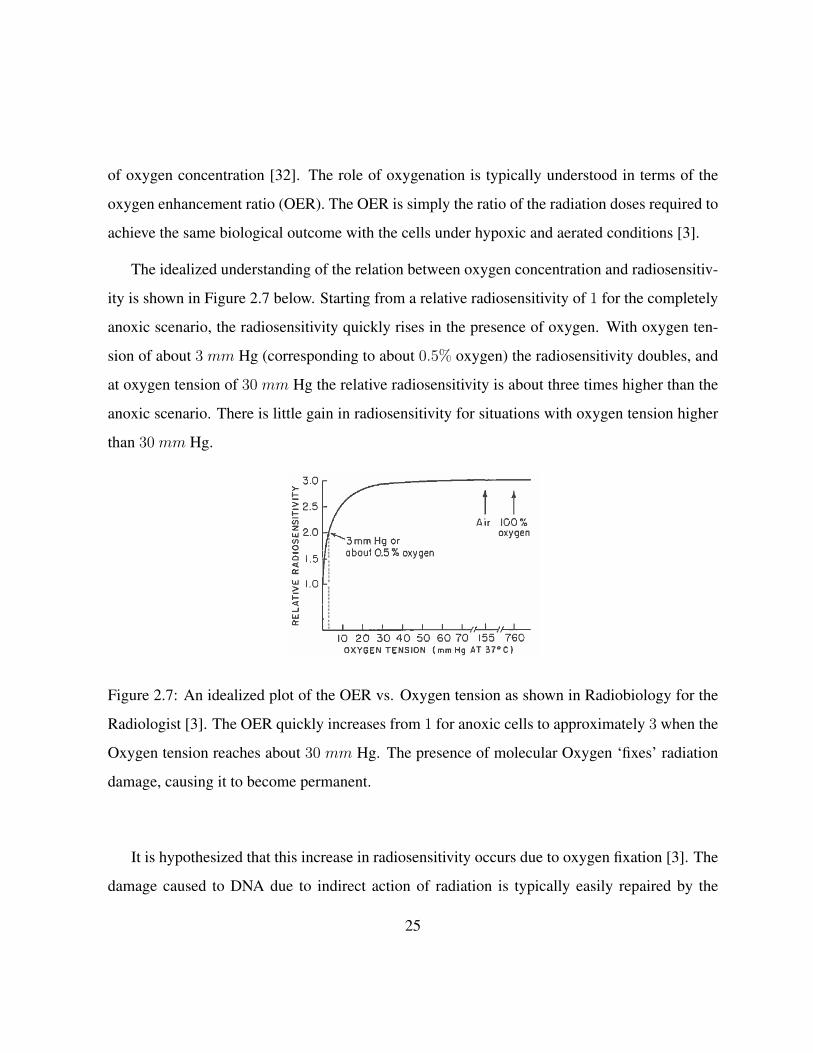
The idealized understanding of the relation between oxygen concentration and radiosensitiv-

ity is shown in Figure 2.7 below. Starting from a relative radiosensitivity of 1 for the completely

anoxic scenario, the radiosensitivity quickly rises in the presence of oxygen. With oxygen ten-

sion of about 3 mm Hg (corresponding to about 0.5% oxygen) the radiosensitivity doubles, and

at oxygen tension of 30 mm Hg the relative radiosensitivity is about three times higher than the

anoxic scenario. There is little gain in radiosensitivity for situations with oxygen tension higher

than 30 mm Hg.

Figure 2.7: An idealized plot of the OER vs. Oxygen tension as shown in Radiobiology for the

Radiologist [3]. The OER quickly increases from 1 for anoxic cells to approximately 3 when the

Oxygen tension reaches about 30 mm Hg. The presence of molecular Oxygen ‘fixes’ radiation

damage, causing it to become permanent.

It is hypothesized that this increase in radiosensitivity occurs due to oxygen fixation [3]. The

damage caused to DNA due to indirect action of radiation is typically easily repaired by the

25

cell, especially in anoxic situations. However, molecular oxygen readily reacts with the site of

damage on the DNA strand, causing the damage to be permanent. Therefore, when molecular

oxygen is available to react with damage to the DNA, more permanent damage to the DNA

occurs, resulting in more cell death and greater radiosensitivity.

Reoxygenation is the process by which hypoxic tumour cells become oxygenated after a tu-

mour receives a dose of radiation. This process occurs due to the usual structure of a tumour

mass. The organization of cells in a tumour is haphazard (compared to healthy tissue) and there-

fore the transfer of nutrients throughout a larger tumour is poor. This results in ‘typical’ tumour

structure with three layers: a layer of aerobic cells surrounding a layer of hypoxic cells which

in turn surround a necrotic core at the center of the tumour. After irradiation, the aerobic cells

on the exterior of the tumour will be preferentially killed due to increased radiosensitivity. As

these cells die off and are removed by bodily systems, oxygen is able to penetrate deeper into the

tumour, thereby reoxygenating previously hypoxic cells. When the next fraction of radiotherapy

is delivered, the previously hypoxic cells will now be more radiosensitive due to reoxygenation.

With repeated delivery of fractionated radiotherapy, the reoxygenation effect can be exploited to

increase cell killing for an equal delivered dose.

26

Figure 2.8: A depiction of the reoxygenation process as shown in Radiobiology for the Radi-

ologist [3]. The oxygenated cells on the exterior of the tumour are more radiosensitive and are

preferentially killed. As the previously hypoxic cells become reoxygenated, their radiosensitivity

increases, making them more susceptible to radiation damage during the next treatment fraction.

Redistribution

Redistribution in the context of radiobiology refers to the distribution of cells across the various

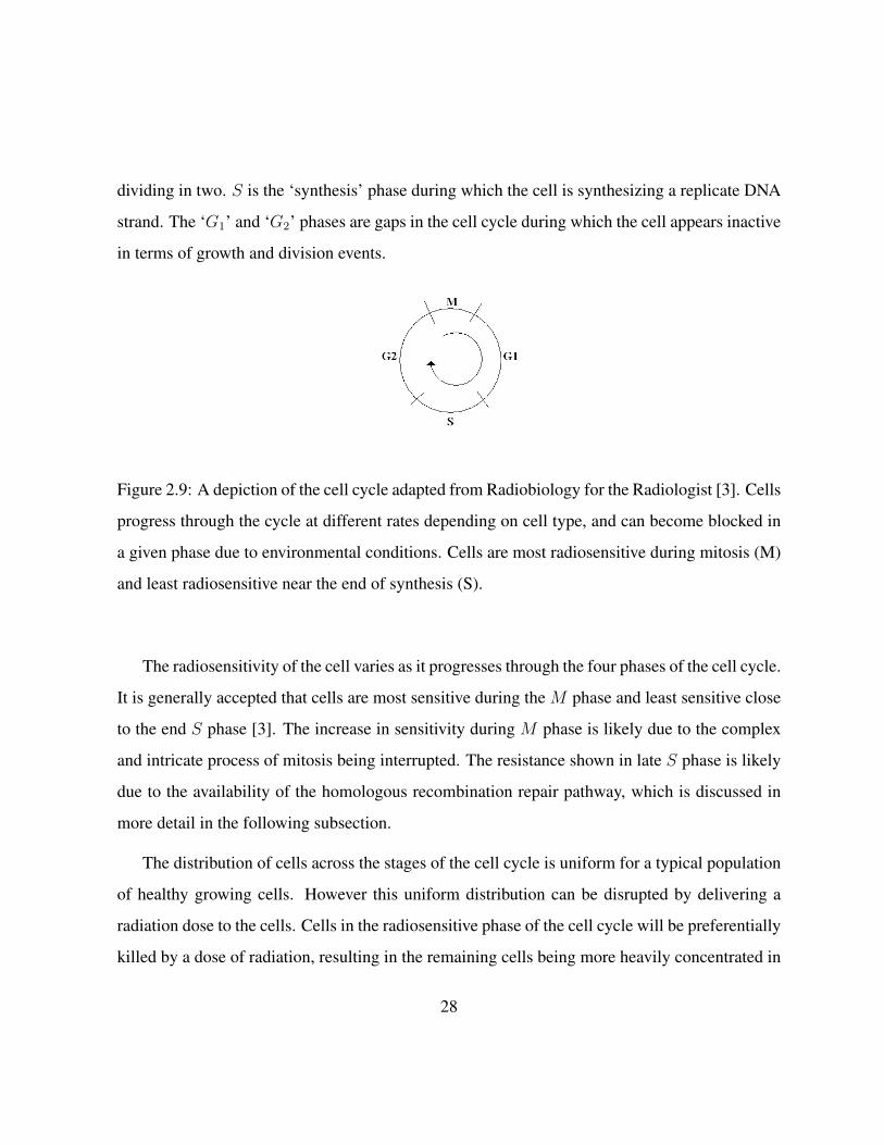
stages of the cell cycle. For mammalian cells, the cell cycle, as shown in Figure 2.9 is divided

into four phases labeled: M ,G1, S,G2. M is the ‘mitosis’ phase during which the cell is actively

27

dividing in two. S is the ‘synthesis’ phase during which the cell is synthesizing a replicate DNA

strand. The ‘G1’ and ‘G2’ phases are gaps in the cell cycle during which the cell appears inactive

in terms of growth and division events.

Figure 2.9: A depiction of the cell cycle adapted from Radiobiology for the Radiologist [3]. Cells

progress through the cycle at different rates depending on cell type, and can become blocked in

a given phase due to environmental conditions. Cells are most radiosensitive during mitosis (M)

and least radiosensitive near the end of synthesis (S).

The radiosensitivity of the cell varies as it progresses through the four phases of the cell cycle.

It is generally accepted that cells are most sensitive during the M phase and least sensitive close

to the end S phase [3]. The increase in sensitivity during M phase is likely due to the complex

and intricate process of mitosis being interrupted. The resistance shown in late S phase is likely

due to the availability of the homologous recombination repair pathway, which is discussed in

more detail in the following subsection.

The distribution of cells across the stages of the cell cycle is uniform for a typical population

of healthy growing cells. However this uniform distribution can be disrupted by delivering a

radiation dose to the cells. Cells in the radiosensitive phase of the cell cycle will be preferentially

killed by a dose of radiation, resulting in the remaining cells being more heavily concentrated in

28

the radioresistant phases. The remaining cells will then proceed through the cell cycle, naturally

redistributing themselves into more radiosensitive phases one again. This redistribution acts to

sensitize the cell population to a future dose of radiation.

Repair

Radiation damage to cells can be classified in one of three categories: lethal damage, poten-

tially lethal damage (PLD) and sublethal damage (SLD). Lethal damage is irreparable and leads

directly to cell death by definition, PLD is damage that is subject to influence by the local en-

vironmental conditions the cells face after irradiation, and SLD is damage that can be reliably

repaired by the cell over the course of hours under normal conditions [3].

Lethal radiation damage to cells usually takes the form of DSBs. However there are two

processes by which the cell may attempt to repair a DSB, known as homologous recombina-

tion repair (HRR) and nonhomologous end joining (NHEJ) [3]. HRR is a very reliable repair

mechanism that uses an undamaged DNA strand as the template for repair of the broken DNA

strand. This repair pathway occurs most frequently in the late S or G2 phase of the cell cycle.

The NHEJ repair pathway for DSBs does not require an undamaged template. Instead, the repair

mechanism is able to identify the broken ends of the DNA strand, prepare the ends for repair,

‘bridge’ the broken ends with the required base pairs and then reattach the broken ends through

the process of ligation. While both pathways result in the reliable repair of DSB, they are not

perfect and can occasionally lead to faulty repairs resulting in chromosomal aberrations. These

aberrations may ultimately cause cell death or hereditary disease.

PLD is damage that would usually cause cell death, but may be overcome under certain local

environmental conditions of the cell. The general consensus is that PLD can be repaired when

the conditions for cell growth are poor [3]. In this situation, the cell will not be likely to undergo

29

the taxing process of mitosis. Instead the cell’s resources can be put towards the necessary DNA

repair. This form of damage was described by Little et al. [33] in an in vitro experiment. The

group showed that a greater fraction of cells survive replating if they are held in a stationary

state (poor growth conditions) for at least 6 hours post irradiation as compared to the fraction of

cells that survive replating immediately after irradiation. It was later shown that the rate of repair

and repair pathways involved in the in vitro experiment are comparable to the in vivo situation.

Although the existence of PLD is widely accepted, its role in radiotherapy is not generally agreed

upon [3].

SLD is damage that would usually be repaired by the cell. The repair of SLD can be observed

in experiments that divide a given radiation dose into two fractions spaced apart in time. Shown

in Figure 2.10 is a plot of the surviving fraction of cells versus the time interval between two

equal doses of radiation adapted from Elkind et al. [34]. By allowing for as little as 30 min-

utes between irradiations, the surviving fractions is appreciably higher. After about two hours

between fractions, the gain in cell survival plateaus. The increase in cell survival in the approxi-

mately two hours post irradiation is understood to be due to the repair of SLD. The hypothesis is

that cell survival is decreased by compounding multiple events that would normally result in SLD

on their own. Therefore, by allowing time between fractions, SLD is repaired before multiple

SLD events can be accumulated in the same region of the DNA strand.

30

Figure 2.10: A plot of the surviving fraction of cells after two doses of radiation separated in

time (7.63 Gy followed by 7.95 Gy). The data are adapted from the experiments performed by

Elkind et al. [34] with Chinese hamster cells incubated at 24 ◦C. The surviving fraction increases

rapidly when the time between doses allows for SLD repair.

Repopulation

Repopulation simply refers to the growth of new cells, whether cancerous or normal, over the

course of a radiotherapy treatment. Work done by Fowler et al. showed that extra radiation dose

is required to counteract the proliferation of new cells [35]. However, it is necessary to consider

the effect of repopulation in the context of the early and late responding tissues discussed earlier.

Early responding tissues in humans with a high α/β ratio are triggered to start proliferating

31

within a few weeks of the start of a fractionated radiotherapy regime. As a result the extra

dose needed to compensate for this proliferation is not required initially, but does increase over

time. On the other hand, late responding tissues will not begin proliferating within the typical

6 − 8 week time frame of a fractionated radiotherapy regime. Therefore, as stated by Hall

[3] ‘prolonging overall time within the normal radiotherapy range has little sparing effect on late

reactions but a large sparing effect on early reactions’. This must be balanced with the knowledge

that excessive prolongation of the fractionation scheme could allow for the tumour cells to begin

proliferating during the treatment.

2.4.5 Tumour Control Probability and Normal Tissue Complication Prob-

ability

Tumor Control Probability (TCP) as originally described by Munro et al. [36] is defined as

the probability that the elimination of all tumour cells has been achieved. Webb et al. [37]

later derived an expression for TCP based on the survival of cells exposed to a uniform dose of

radiation. Where the number of surviving cells is given by the familiar LQ model (the quadratic

term is omitted while considering the typical radiotherapy fraction size of ' 2 Gy)

S = e−αD. (2.11)

The probability of eliminating all the tumour cells is then simply given by

TCP = e−S. (2.12)

When the TCP is plotted as a function of dose, the resulting curve is sigmoidal in nature with

increasing dose resulting in an increased probability of tumour control. However, increasing

32

the dose is also associated with an increase in normal tissue complication probability (NTCP).

Perhaps the most popular model of NTCP was developed by Lyman [38] and expanded upon by

Burman et al. [39]. The basis of the so-call LKB model of NTCP is an error function and four

parameters defined by the following equations:

NTCP =1√2π

∫ t

−∞e−t

2/2dt, (2.13)

ν = V/Vref , (2.14)

t =D − TD50(ν)

(m× TD50(ν)), (2.15)

TD(ν) = TD(1)× ν − n. (2.16)

The parameter ν is defined as the fraction of the organ irradiated (or the proportion relative to

a reference volume), D is the dose, TD50 is the tolerance dose resulting in a 50% complication

probability, n is the parameter governing the volume dependence of the complication probability

and m is the parameter governing the slope of the curve (at 50% complication probability).

It should be noted that when the NTCP is plotted as a function of dose, it is monotonically

increasing [39]. Therefore any increase in dose to the healthy tissues of the patient will increase

the probability of complication. Similarly, when NTCP is plotted as a function of the partial

volume of the irradiated tissue, it is also monotonically increasing [39]. Therefore, any increase

in the volume of normal tissue being irradiated to a given dose will also increase complication

probability. These two considerations are at the heart of treatment planning. The ideal treatment

33

plan balances the delivery of the prescribed dose to the target volume with the volume and dose

of irradiated normal tissues.

When plotted together versus the delivered dose, both the TCP and NTCP appear as sigmoidal

curves separated along the dose axis. Figure 2.11 shows the plot in a hypothetical situation. A

given dose will result in a given probability for NTCP and TCP. The difference in the relative

responses of the tissues to a given dose is termed the ‘therapeutic advantage’. The outcomes

of radiotherapy treatments can be improved by increasing the therapeutic advantage. The TCP

and NTCP curves can be shifted along the dose axis through several means, such as: the action

of any of the 4 R’s, by radiosensitizing the tumour with a chemical agent or by increasing the

radioresistance of the OARs.

34

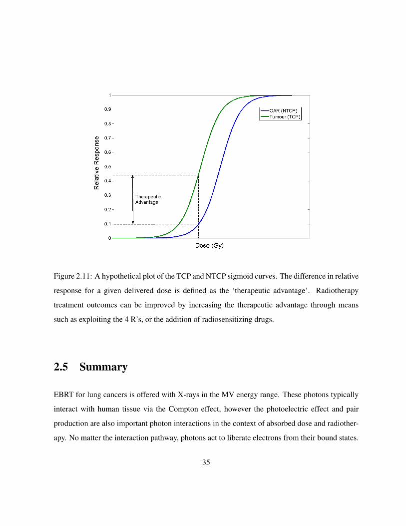
Figure 2.11: A hypothetical plot of the TCP and NTCP sigmoid curves. The difference in relative

response for a given delivered dose is defined as the ‘therapeutic advantage’. Radiotherapy

treatment outcomes can be improved by increasing the therapeutic advantage through means

such as exploiting the 4 R’s, or the addition of radiosensitizing drugs.

2.5 Summary

EBRT for lung cancers is offered with X-rays in the MV energy range. These photons typically

interact with human tissue via the Compton effect, however the photoelectric effect and pair

production are also important photon interactions in the context of absorbed dose and radiother-

apy. No matter the interaction pathway, photons act to liberate electrons from their bound states.

35

These free electrons are responsible for the deposition of all the energy comprising the absorbed

dose to tissue. The energy absorbed by the tissue will result in ionizations to the constituent

atoms and molecules of the tissue. These ionized atoms and molecules are chemically reactive.

When the DNA itself is ionized, or a atom/molecule nearby the DNA is ionized, they will become

chemically reactive. The result of the chemical activity can be a break in the backbone strand of

the DNA molecule. In the cases where this damage is irreparable, the result is often cell death.

The study of radiobiology has allowed for the honing of radiotherapy techniques. The four

‘R’s’ of radiobiology (Reoxygenation, Redistribution, Repair and Repopulation) form the ba-

sis of our understanding of the biological outcomes associated with the delivery of a specific

dose. The study of the survival rate of cells exposed to radiation has lead to the commonly used

Linear-Quadratic model of cell survival, which has often served as the basis of tumour control

probabilities (TCP) and normal tissue complication probabilities (NTCP). The study and under-

standing of photon interactions and radiobiology forms the basis of modern radiotherapy.

36

Chapter 3

Review of Radiation Therapy for Lung

Cancers

3.1 Introduction

Each tumour site presents with its own unique challenges for the planning and delivery of exter-

nal beam radiation therapy (EBRT). Usually, the need to limit dose to the OARs in the region of

a given tumour will pose the biggest challenge to delivering a high dose to the tumour. However,

organ motion also presents challenges to the accurate delivery of EBRT. Although any given

treatment site may be susceptible to organ motion (both interfraction and intrafraction), the res-

piratory motion of the lungs causes displacement of lung tumours greater than that routinely seen

at any other treatment site.

The treatment of lung cancers with EBRT is also complicated by challenges with accurate

dose calculation. Due to differences in tissue density between healthy lung tissue and a tumour

within the lung, it is difficult to model the dose, especially in the interface region. Furthermore,

37

the relatively low density of lung tissue allows for increased lateral electron disequilibrium which

is not typically an important consideration at other treatment sites.

Many approaches have been developed by researchers and clinicians to deal with the chal-

lenges of EBRT for lung cancers. This chapter aims to discuss lung cancer in the context of

EBRT, approaches to quantifying lung target motion and approaches to accounting for that mo-

tion in treatment planning and delivery. Finally, a closer look at the margin recommendations

made by other authors in the literature is provided.

3.2 Classification of Lung Cancers

Lung cancer is the leading cause of cancer death in Ontario for both men and women. Approx-

imately 1 in 4 cancer deaths in Ontario result from lung cancer [40]. Therefore, the prevention

and treatment of lung cancers is a high priority for clinicians in the provincial health system.

There exists many different types of lung cancer, but they can be broadly classified into small

cell lung cancer (SCLC) and non-small cell lung cancer (NSCLC) groups.

SCLC represents approximately 15% of lung cancer cases but also account for 25% of lung

cancer deaths [41]. These cancers are typically much more difficult to treat due to rapid cell

division and the propensity to metastasize early in the development of the disease. SCLC are

most often found centrally within the lung, usually originating in the bronchi. Cigarette smoking

is implicated as the cause of up to 95% of SCLC cases [42]. The treatment regime for SCLC

is dependent on the stage of the disease, but will usually be a combined modality treatment of

chemotherapy and radiation therapy. The metastatic potential of SCLC means that surgery is not

typically offered for treatment of SCLC. Limited stage disease (confined to a single lobe of the

lung) has much better survival rate than extensive disease, with a 5-year survival rate of limited

38

stage SCLC patients of 20%. The long term survival rates for patients diagnosed with extensive

SCLC is very low, with the median survival length in the range of 8 to 10 months.

NSCLC comprises the other 85% of lung cancer cases [43]. NSCLC does not typically grow

or metastasize as quickly as SCLC. As such, NSCLC is seen as more treatable and has better

survival rates (5-year survival of approximately 15%). Cigarette smoking is again the most com-

mon cause of NSCLC, although environmental factors such as air pollution are implicated in up

to 11% of cases in some regions [43]. Surgery is the mainstay treatment for NSCLC with com-

plete resection and wedge resection frequently being offered. Almost 70% of patients initially

present with locally advanced or metastatic disease, and for these people chemotherapy in combi-

nation with surgery is typically offered. Radiation therapy for NSCLC patients is conventionally

offered in a regime of 60 Gy delivered in 30 daily fractions. The Radiation Therapy Oncology

Group (RTOG) performed a phase 3 trial for locally advanced, non-resectable NSCLC which

resulted in local failure rates of 27%. However conventional radiation therapy alone results in a

median survival of 10 months and 5-year survival rate of only 5% for this group. New radiation

therapy techniques, such as stereotactic body radiation therapy for treating early stage NSCLC

has shown promise, with one trial offering local control to 87.2% of patients [44].

3.3 Staging of Lung Cancers

The diagnosis and staging of lung cancer is a key step in determining the appropriate treatment

regime. A computed tomography (CT) scan of the chest is most often used in the initial diagnosis

of lung cancer. Additional testing, such as a complete blood cell count and electrolyte panel

can be used to discriminate between SCLC and NSCLC. Since CT has limited ability to detect

microscopic metastatic disease, radionuclide scans such as positron emission tomography (PET),

are also being used as part of the modern diagnosis of lung cancer. PET scans allow for the

39

detection of the highly active cells typical of cancers and can be used to detect the metastatic

activity that may be missed by a CT scan. Ultimately it is a combination of tests that leads to the

diagnosis and staging of lung cancer. The stages of lung cancer are classified by TNM system,

where a score is assigned to each of: T - the size and location of the tumour, N - the lymph

node involvement and M - the metastatic state of the disease. The stages and TNM scores are

described below as defined by the System for Staging Lung Cancer [45]. Later stage cancers

have a worse prognosis.

Stage IA (T1N0M0) & IB (T2N0M0): These are the earliest stages which are commonly

diagnosed. The N0 and M0 designations refer to the fact that there is no apparent lymph node

involvement or metastatic spread of the disease. The T1 designation is for cancers which are

≤ 3 cm in their greatest dimension. T2 tumours have at least one of the following characteristics:

dimension > 3 cm, limited involvement with the main bronchus, have caused a partial collapse

of the lung or have caused obstructive pneumonitis. Lung cancers in stage IA and IB are most

commonly treated with surgical resection. Patients in this stage who are not amenable to surgery

may benefit from stereotactic radiosurgery.

Stage IIA (T1N1M0) & IIB (T2N1M0, T3N0M0): Stage II lung cancers are also most com-

monly treated with surgery and chemotherapy. The N1 designation denotes spread of the disease

into the ipsilateral peribronchial and hilar lymph nodes. The T3 designation is for tumours of

any size that are invading the structures surrounding the lung such as the: chest wall, diaphragm,

pericardium. A T3 designation would also be given to a tumour causing a complete collapse of

the lung.

Stage IIIA (T3N1M0, T1/2/3N2M0) & IIIB (T4N0/1/2M0, T1/2/3/4N3M0): Patients diag-

nosed with stage III lung cancers have poor prognosis with 5-year survival rates in the 6-9%

range. The N2 designation is for mediastinal and/or subcarinal lymph node involvment while the

N3 designation is for contralateral lymph node involvement. The T4 designation is for tumours

40

of any size that involve the critical surrounding organs such as the: heart, mediastinum, great

vessels, trachea, esophagus or vertabrae. A tumour would also be classified as T4 in the case

of multiple ipsilateral tumour nodules. Treatment for stage III lung cancer will typically be a

combined modality approach, however in some cases the only option is for palliative treatment

(often including radiation therapy) to relieve suffering.

Stage IV (Any T, Any N, M1): Any lung cancer that has metastasized to a distal region of

the body (M1) is given a stage IV classification. These patients have the worst prognosis with

5-year survival of approximately 1%. Palliative treatment would be offered to these patients in

most cases, as a curative approach will most likely fail.

3.4 Radiotherapy of Lung Cancers

There are many considerations that must be taken when delivering radiotherapy to any cancer

site within the body, including the dose prescription and delivery technique, dose to OARs and

our ability to employ accurate dose calculation algorithms. Lung cancer presents some unique

challenges in these areas due to the natural radioresistance of lung cancer cells, the location of

the cancer within the body relative to other organs, the physical density of lung tissue and lung

motion due to respiration.

When radiotherapy is indicated for the treatment of lung cancer, the most common treatment

regime being offered today is to deliver 60 Gy in 30 daily fractions (2 Gy per fraction) to the

treatment volume. This regime was developed and tested by the RTOG in a phase III dose

escalation trial published in 1995 [46]. Ultimately this standard of care was shown to limit

local failure rates to approximately 27%. However, since that time many other approaches have

been tested for lung cancers at various stages. One such approach for earlier stage cancers is

41

known as stereotactic body radiation therapy, which delivers up to 18 Gy per fraction in as

few as 3 fractions [44]. In this case the authors reported high rates of local control (97.6%

at 3 years), 55.8% survival at 3 years and only moderate treatment related toxicity. Different

treatment regimes are routinely being tested for lung cancers of different stages, with new options

becoming available as technology improves.

3.4.1 Organs at Risk

No matter what treatment regime is selected to treat a lung cancer, careful consideration must

be given to the dose being delivered to the OARs. The location of the lungs within the chest

put several critical structures in the vicinity of lung cancers, such as the: heart, spinal cord,

and esophagus. The skin, ribs, breast (in women) and the lungs themselves are also at risk for

radiation damage during treatment. The dose constraints to each of these OARs is dependent

on the fractionation scheme, the toxicity endpoint, the rate at which the endpoint is met and the

use of other treatment modalities. As a result many dose constraint recommendations have been

published, with the data from Emami et al. [47], QUANTEC [48] and various RTOG protocols

most commonly referenced. Table 3.1 summarizes the dose constraints to the common lung

radiotherapy OARs.

42

OAR Volume (%) Dose Toxicity Rate Toxicity Endpoint

Heart [49] Mean < 26 Gy < 15% Pericarditis

Spinal cord [50] Max < 50 Gy 0.2% Myelopathy

Esophagus [51] Mean < 34 Gy 5− 20% Grade 3+ esophagitis

Lung [48] Mean < 20 Gy < 20% Pneumonitis

Lung [48] V20 < 30% < 20% Pneumonitis

Table 3.1: Dose constraints for various OARs common to lung EBRT. The data presented here

are taken from the QUANTEC series published in 2010. These constraints represent guidelines

as specific constraints depend on many patient specific factors.

Modern imaging and planning tools allow for the selection of X-ray beam angles to avoid

many of these structures by providing an accurate and detailed map of the patient anatomy and

its position relative to the treatment beam. As a result, major complications from radiation side

effects are less frequent than in the past and the most common form of toxicity found in pa-

tients is radiation pneumonitis of the lungs [52]. Radiation pneumonitis is an early complication

characterized by the development of a dry cough and shortness of breath. The late complication

associated with pneumonitis is known as fibrosis. Fibrosis is a scarring of the lung tissue as a re-

sult of radiation damage. This damaged lung tissue becomes more dense, less flexible and much

less effective at exchanging gases between the atmosphere and blood. Radiation pneumonitis

and fibrosis leads to a further shortness of breath in patients who already typically have trou-

ble breathing due to their condition. In 2010 a comprehensive review of radiation toxicity was

published under the name QUANTEC. In considering radiation damage to the lung, the authors

pointed to the mean lung dose (MLD) as the best predictor of radiation pneumonitis [48]. They

recommended limiting the MLD to ≤ 20 − 23 Gy as well as limiting the percentage of lung

43

volume receiving ≥ 20 Gy to ≤ 30− 35% (V20 ≤ 30− 35%).

3.4.2 Dose Calculation in Lung

Absorbed dose calculation for targets in the lung is complicated by the changes in tissue density

along the path of the X-ray beam as it enters the body, travels through lung tissue and arrives at

the tumour. As X-rays travel across the interface between tissues of heterogeneous density (such

as the soft tissue surrounding the lungs and the low density lung tissue) the interaction probability

changes. When going from higher density tissue to lower density tissue, the probability of photon

interactions within the tissue drops, and as a result fewer electrons are liberated. This abrupt

change in interaction probability complicates the dose calculation. As the X-rays travel from

low density lung tissue into the higher density tumour mass, an abrupt change in interaction

probability will again occur at the interface. Many clinical dose calculation algorithms have a

difficult time modeling the dose at the interface regions due to their calculation methods. Some

popular algorithms are discussed below.

During regular clinical operation, dose distributions are calculated within commercial treat-

ment planning software (TPS). Varian’s Eclipse TPS uses the Analytical Anisotropic Algorithm

(AAA) which is convolution-superposition (CS) based algorithm for photon dose calculation

[53]. While the fine details of the dose calculation algorithm are proprietary, the basis of the

algorithm is public knowledge [54]. The CS algorithm is a model based algorithm, which means

it calculates the dose directly in a model of the patient (from a CT data set). In order to calculate

the dose at a given point, the CS algorithm first requires data regarding the energy fluence of the

specific beam of interest. From the energy fluence and the mass attenuation coefficient provided

by the CT data set, the total energy released in matter (TERMA) is calculated within the patient

model. The dose calculation is then performed by taking the mathematical convolution of the

44

TERMA with a dose spread kernel. The dose spread kernel describes the dose distribution re-

sulting from a narrow photon beam in water and is originally calculated using Monte Carlo (MC)

methods. The result of the convolution is then superimposed with the convolutions performed at

other points within the patient model to determine the final dose distribution.

The CS dose calculation algorithms are advantageous because they give reliable results under

most conditions with reasonably short calculation times. However, CS algorithms have been

shown to provide inaccurate results in situations with low tissue density, high energy beams and

tissue inhomogeneities depending on the size of the beam and the beam energy [55]. Of particular

interest to lung is the problem of lateral electron disequilibrium. Due to the low density of lung

tissue, the path length of a given electron traveling through lung will be longer than that of an

electron in unit density material (the basis of the CS algorithm). As a result, electrons may travel

much further laterally (perpendicular to the beam direction) in lung than is actually accounted

for by the dose spread kernel in the CS algorithm. Electrons which travel outside the beam

profile will deposit their energy in unintended structures. This generally leads to CS algorithms

underestimating dose to surrounding healthy tissue in the lung and overestimating dose in the

target volume. Furthermore, since the dose spread kernel does not account for heterogeneities in

the mass attenuation map of the patient, the CS model is prone to dose calculation errors at the

interface of heterogeneous tissues.

In order to circumvent these issues and achieve highly accurate estimates of absorbed dose,

other calculation methods must be employed, namely MC methods. MC simulations track the

path and energy deposition of a huge number of virtual particles in order to determine absorbed

dose in a given volume. By relying on a very large sample size of simulated particle interactions,

MC simulation offers accurate dose calculations at the expense of large computing power. MC

work published in 2012 [56] shows that in some extreme circumstances, electron disequilibrium

can contribute to large differences (up to 20%) in the dose calculated with typical CS algorithms.

45

Other groups have shown that for small lung targets (stage I), commonly used dose calcula-

tion algorithms (AAA and AcurosXB) underestimate the dose by approximately 12%, while the

difference is much smaller (0.8%) for stage III lung targets [57]. While MC dose calculation

is generally considered the ‘gold standard’ for dose calculation, the slow calculation times and

large computing power required have prevented MC from being used in regular clinical settings.

3.5 Quantifying Target Motion in the Lung

Treating lung cancers with EBRT is further complicated by the motion of the lungs caused by pa-

tient respiration. If conventional imaging, treatment planning and treatment delivery techniques

are used, motion induced complications in the treatment process arise at each stage. Webb pub-

lished a thorough review of motion effects and treatment techniques in radiation therapy [58]. In

order to adequately compensate for this motion and deliver a successful treatment, a thorough

understanding of the motion is required. The least invasive approach to measuring target motion

in the lung is with medical imaging techniques, namely fluoroscopy, CT, and magnetic resonance

imaging (MRI).

Initial attempts at quantifying target motion in the lung were performed using fluoroscopic

imaging. Fluoroscopy uses continuous exposures of X-rays to generate sequential 2D digital

images of the patient anatomy. While fluoroscopic images usually suffer from low contrast,

the low density of healthy lung tissue (relative to other soft tissues) makes it feasible to detect

and delineate lung cancers in fluoroscopic images. One early attempt at quantifying lung target

motion was published by Ekberg et al. [18]. The authors studied the motion of lung targets

using an electronic portal imaging device (EPID) to detect motion on the treatment unit. They

ultimately used their data to make margin recommendations as well.

In 2003 Vedam et al. [20] published an article quantifying the predictability of diaphragm

46

motion. The authors used fluoroscopy to track the position of the diaphragm while having pa-

tients (1) breathe freely, (2) breathe with audio prompting, and (3) breathe with video prompting.

The authors found that free breathing patients have diaphragm position variability similar to that

of patients receiving video prompting and less variability than patients receiving audio prompt-

ing. This confirmed the earlier results of Mageras et al. who performed a similar study [59].

Although it is generally considered that lung target motion is greatest in the superior-inferior

(SI) direction within the patient, target motion does occur in all three principal directions. Due

to the 2D views provided by fluoroscopic approaches, it is impossible to measure displacements

in all three directions from a single set of images. The ability to measure target displacement in

3D is one of the major advantages offered by CT and MRI patient scans. The details of 4DCT

scans are discussed later in this chapter, but it is important to note some contributions made to

quantifying target motion in the lung that have been made with 4D scans.

A work published by Shirato et al. [11] used 4DCT scans with implanted fiducial markers to

detect tumour speed and location using 4DCT. The use of fiducial markers reduces uncertainty

associated with delineating target volumes with low contrast images. However, implanting fidu-

cial markers is an invasive procedure that may not be well tolerated by all patients. Bissonnette

et al. [60] investigated interfraction and intrafraction using respiration-correlated cone beam CT

(rcCBCT). They were able to assess how target motion changed during treatment by acquiring

rcCBCT images before daily treatment, at the midpoint of the treatment and the end of treatment.

They showed no statistical difference in tumour motion magnitude over the course of a treatment

delivery of the patients studied. Shirato et al. studied 21 patients and were able to detect tumour

displacement and speed in each of the three principal directions by using 4DCT. In a work pub-

lished by Mageras et al. [61] the authors were able to detect the motion of lung tumours without

the use of fiducial markers. The authors noted that some tumours followed a trajectory which

included some hysteresis. Mageras et al. also derived some margin recommendations from their

47

study of lung target motion. Finally, a detailed work analyzing the motion of lung tumours using

MRI was published by Plathow et al. in 2004 [62]. The authors were able to study the 3D motion

of targets in each of the different lobes of the lung. Plathow et al. concluded that tumours in the

lower lobes moved significantly more than tumours in the upper lobes. They were also able to

establish the fact that regions of the lung which are involved in the disease are less mobile than

the healthy regions of the lung.

Many other authors have also studied the motion of targets in the lung and have reported

valuable data regarding the ranges of amplitude and direction of displacement. A summary of

select published results is presented in Table 3.2. Some of the results in the summary table are

divided into the region of the lung where the tumour is located. Due to the mechanics of the

breathing motion, targets in the lower lobes of the lungs are more susceptible to motion.

Perhaps the most important point to note about target motion in the lung is that there is a

wide range of motion presented by different patients. As can be seen in Table 3.2, there have

been many studies performed, all with different values recorded for the amplitude of motion.

This reinforces the need to measure and verify tumour motion in the lung on a patient-by-patient

basis.

3.5.1 Breathing Traces and Correlation to Target Motion

Taking a recording of a given patient’s breathing pattern is an important step toward adapting

the radiotherapy treatment to their specific anatomy. This issue has been tackled by many au-

thors using several different approaches. The most common approaches involve measuring the

displacement of the exterior chest wall while the patient is in the treatment position. This can be

accomplished using different technologies such as an elastic belt with embedded pressure sensor

(e.g. AZ-733V Respiratory Gating System from Anzai Medical Co., Tokyo, JP) [65, 66], or with

48

Direction of Target Motion

Author & year SI AP LR

Ekberg 1998 [18] 3.9 (0-12) 2.4 (0-5) 2.4 (0-5)

Engelsman 2001 [19](2-6) Upper lobe - -

(2-9) Lower lobe - -

Seppenwoolde 2002 [9] 5.8 2.5 1.5

Murphy 2002 [63] 7.0 (2-15) - -

Sixel 2003 [10] (0-13) (0-5) (0-4)

Plathow 2004 [62]

4.3 (2.6-7.1) Upper lobe 2.8 (1.2-5.1) 3.4 (1.3-5.3)

7.2 (4.3-10.2) Middle lobe 4.3 (1.9-7.5) 4.3 (1.5-7.1)

9.5 (4.5-16.4) Lower lobe 6.1 (2.5-9.8) 6.0 (2.9-9.8)

Shirato 2006 [11] 10.7 8.8 8.2

Liu 2007 [15] 13.4 5.9 4.0

Suh 2008 [64]3.7 Upper lobe

- -8.0 Lower lobe

Table 3.2: Average (or ranges) of lung target motions reported in millimeters along the principle

body directions: superior-inferior (SI), anterior-posterior (AP), left-right (LR).

49

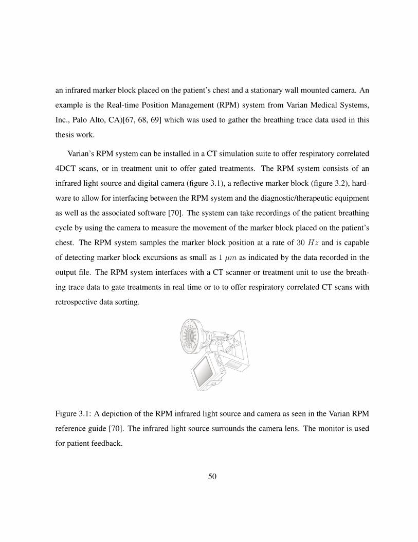
an infrared marker block placed on the patient’s chest and a stationary wall mounted camera. An

example is the Real-time Position Management (RPM) system from Varian Medical Systems,

Inc., Palo Alto, CA)[67, 68, 69] which was used to gather the breathing trace data used in this

thesis work.

Varian’s RPM system can be installed in a CT simulation suite to offer respiratory correlated

4DCT scans, or in treatment unit to offer gated treatments. The RPM system consists of an

infrared light source and digital camera (figure 3.1), a reflective marker block (figure 3.2), hard-

ware to allow for interfacing between the RPM system and the diagnostic/therapeutic equipment

as well as the associated software [70]. The system can take recordings of the patient breathing

cycle by using the camera to measure the movement of the marker block placed on the patient’s

chest. The RPM system samples the marker block position at a rate of 30 Hz and is capable

of detecting marker block excursions as small as 1 µm as indicated by the data recorded in the

output file. The RPM system interfaces with a CT scanner or treatment unit to use the breath-

ing trace data to gate treatments in real time or to to offer respiratory correlated CT scans with

retrospective data sorting.

Figure 3.1: A depiction of the RPM infrared light source and camera as seen in the Varian RPM

reference guide [70]. The infrared light source surrounds the camera lens. The monitor is used

for patient feedback.

50

Figure 3.2: A depiction of the RPM infrared marker block as seen in the Varian RPM reference

guide [70]. The markers reflect the infrared light from the camera source. In order to offer

accurate measurement, the infrared signal from the reflective block must be the strongest signal

in the room.

In order to provide information regarding the location of a target within the patient, any ex-

ternal surrogate system will rely on the correlation between the reading of the surrogate and the

internal phase of the respiratory cycle. Hoisak et al. [8] showed that the reliability of this correla-

tion varies from day to day among patients. The difference between the breathing phase and the

target motion phase can be quantified with a phase angle difference. Redmond et al. [71] found

average changes in the phase angle between the target motion and surrogate of 13.2% and 14.3%

compared to the initial 4DCT during subsequent rescans. Redmond et al. also confirmed the

51

results of Hoisak et al. regarding the reliability of the correlation from day to day. Importantly,

Redmond et al. [71] showed that the target volume excursions remained stable at subsequent

rescans. Redmond et al. also point out that the correlation of the external surrogate to the target

motion is an important issue for gated treatments, as a drift in the phase angle could easily result

in a geographic miss of the delivered radiation.

The recordings generated from these methods offer insight into the patients breathing pattern

in terms of the regularity of the amplitude and frequency of the breaths being taken. An example

of a regular breathing trace recorded using the RPM system is shown in figure 3.3 while an

irregular breathing trace is shown in figure 3.4. A patient with a regular breathing pattern will

typically spend slightly more time at the full exhale phase of the breathing cycle, while irregular

breathers cannot be consistently described in any broad manner.

52

Figure 3.3: An example of a regular breathing pattern recorded with Varian’s RPM system. The

amplitude of the motion and the frequency of the breathing is consistent across multiple breaths.

These breathing traces offer data which can be used in many ways by clinicians. Ultimately, it

is a recording of the breathing trace that allows for reconstruction of 4DCT image data sets. The

breathing traces can also be used to guide clinical decision making such as treatment technique

or margin selection, which will be discussed later. As can be seen in the plot of the irregular

breathing pattern (3.4), it is not necessarily easy to predict future breathing motion based on a

given breathing trace. This is especially true in the case of lung cancer patients who frequently

have trouble with respiration due to their condition. As a result, it is important to use the breath-

53

ing trace with caution when involving the data in clinical decision making. Purdie et al. [72]

described using cone beam CT images acquired at the immediately prior to treatment, and during

treatment, to reduce setup error and assess intrafraction changes in tumour position.

Figure 3.4: An example of an irregular breathing pattern recorded with Varian’s RPM system.

The amplitude of the motion and the frequency of the breathing are inconsistent across multiple

breaths, while the baseline for motion can also been seen to drift.

3.5.2 Computed Tomography of Lung Cancers in Motion

Using CT imaging to determine the position of tumours is a key step in the process of delivering

EBRT. In order to acquire a clear and accurate representation of the patient many trade-offs

have to be made between parameters such as image resolution, absorbed dose to the patient,

image noise, field of view and scan time due to the physical limitations of the system. Acquiring

54

CT images of the lung is further complicated by the motion of the structure during imaging.

Due to the image reconstruction process used to generate 3D CT datasets, any motion which

occurs during image acquisition of a conventional CT scan will cause motion artifacts in the final

image. Figure 3.5 shows an example of a motion artifact at the bottom of the lung, appearing

as a structure with a wavy edge. This type of artifact causes problems in the planning process

because it makes delineating structures more difficult and can also compromise dose calculation,

depending on the calculation algorithm being used. As a result, different approaches to imaging

lung targets in motion have been developed.

Figure 3.5: An example of a CT image artifact caused by organ motion during image acquisition.

Such artifacts compromise the treatment planning process and need to be avoided.

One such approach to reducing image artifacts is known as a ‘slow scan’. By operating the

CT scanner in a slow method, such that the couch position remains constant across at least one

full breathing cycle, the entire range of target motion during the breathing cycle can be captured

on each slice of the CT image. A slow scan can also be achieved by averaging several CT scans of

the same patient together [73]. The advantage of the slow scan is that the entire range of tumour

55

motion is captured in the final image, although this comes at the expense of slightly increased

dose to the patient and additional blurring due to motion of other structures in the image.

Breath-hold techniques can also be used during CT simulation to reduce respiratory motion

artifacts. CT breath-hold techniques require the patient to hold their breath in order to reduce

artifacts due to respiration. Alternatively the patient may be guided through the breathing cycle

with audio or visual prompts. A work published by Hanley et al. [74] was one of the first

to investigate breath-hold CT scans in the context of radiotherapy for the lung. The authors

compared free breathing scans to breath-hold scans and found that they were able to reliably

reduce the margin of uncertainty associated with the target motion by using deep inspiration

breath-hold (DIBH) during CT simulation. Hanley et al. found that DIBH allowed for an up to

30% reduction in the volume of lung receiving 25 Gy during a 75 Gy treatment.

A final technique used to compensate for lung target motion is the use of maximum intensity

projections (MIP). A MIP is an image (or 3D data set) comprised of the ‘maximum intensity’

values of several individual scans. In the case of a CT MIP, each voxel contains the maximum

electron density of the corresponding voxels in the individual scans. Underberg et al. [75] used

3 separate CT images to generate MIPs for lung EBRT: a full inspiration, full exhalation and

a midventilation scan. By combining the images into a MIP, the full range of tumour motion

becomes apparent. The tumour volume as it appears on the MIP then forms the target volume on

which the treatment planning is performed.

No matter the scanning technique used, the ultimate goal is to generate an image which is

anatomically accurate with an acceptably low amount of noise. Image noise is quantified by

determining the standard deviation of the pixel intensity of an image of a uniform subject (e.g.

a cylindrical water phantom)[25]. Within a uniform region of interest (ROI) of a 2D image, the

image noise can be characterized by

56

σ =

√1

N − 1

∑i,jεROI

(fi,j − f)2, (3.1)

where fi,j are the individual pixel intensities, N is the total number of pixels included in the

sum and f is the average pixel intensity calculated by

f =1

N

∑i,jεROI

fi,j. (3.2)

The pixel intensity is simply the Hounsfield unit (HU) value associated with the given pixel.

Since the HU is a rescaling of the measured linear attenuation coefficient (described in equation

2.3), the image noise is ultimately dependent on the standard deviation of the measured linear

attenuation coefficients of the subject. Ford et al. [76] showed that for an idealized CT scanning

system with isotropic voxel size, the variance in measured linear attenuation coefficient of a

cylindrical object is given by

σ2µ =

π2

12∆x2nangN. (3.3)

In this context ∆x is the voxel side length, nang is the number of projection views used in

the reconstruction and N is the number of photons absorbed per projection, per detector. The

number of photons absorbed, N , is ultimately dependent on many parameters of the scanner

design and X-ray tube operation. N is can be determined by

N =ΦI∆tnWHηe−µd

L, (3.4)

where Φ is the fluence rate per unit tube current at the detector plane, I is the tube current,

∆t is the exposure time per view, n is the number of detector elements per view, W is the

57

aperture width, H is the slice thickness, η is the quantum efficiency of the detector, µ is the

linear attenuation coefficient of the subject, d is the diameter of the subject and L is the number

of reconstruction bins in the image.

Given that the image noise is inversely dependent on the number of photons absorbed by the

detectors (N ), the best way to reduce image noise is to increase the value of N . This can be

achieved by the appropriate manipulation of any of the parameters which comprise N . However,

any increase in the value of N will necessarily increase the effective dose to the patient. This is

the ultimate trade off for CT image quality: if you wish to reduce image noise while maintaining

all other image parameters (e.g. contrast, resolution, scan time), you must increase the dose to

your subject. In a clinical situation, the balance that must be struck is between acceptable image

quality and dose to the patient.

4DCT for Imaging Lung Cancer

Another approach which is growing in popularity as the required technology becomes more

widespread is the use of 4DCT scans. A 4D scan generates multiple (typically 8-10) complete

datasets of the patient, each corresponding to a different phase of the breathing cycle. This

approach offers the benefits of increased contrast (as compared to a slow scan) and the avoidance

of motion artifacts in the images. The datasets may be viewed in sequential order, thus offering

a short movie of the target motion due to respiration.

Modern CT hardware is required to generate a 4DCT scan. These scanners have very fast

gantry speeds (on the order of 1 second per rotation) which allows the machine to acquire a

complete view of the patient in less than the time required for a typical breathing cycle (on the

order of 3 seconds per cycle). The acquired image views must be sorted according to when they

were acquired during the breathing cycle. This is accomplished with the aide of the recorded

58

breathing trace. An early description of the procedure for acquiring a 4DCT scan correlated to

respiratory motion was published by Ford et al. [77]. The images can be sorted according to the

phase of the breathing trace during which they were acquired [78], or according to the amplitude

(position) of a surrogate marker during the breathing cycle [79]. 4D scans come at the expense

of increased dose to the patient and increased workload for the clinical resources [77]. Due to

the rapid acquisition times, the individual phased images will typically have more image noise

as compared to a conventional scan. However, the additional positional information gained by

this method is very valuable during treatment planning.

A 4DCT is similar to a conventional CT scan in most regards. The image data is acquired and

reconstructed in the same overall manner. However, in the case of 4DCT, the X-ray projection

data is recorded along side the patient’s breathing pattern and additional X-ray projections are

acquired to use in a post-processing procedure. After acquiring the data from the scan, the X-ray

projections are sorted into groups depending on which point of the breathing cycle the projection

data was captured. Each of these groups of data are then used to reconstruct an image of the

patient corresponding to the given portion of the breathing cycle. A typical 4DCT scan will

reconstruct 8 − 10 image data sets which can then be viewed in sequence to offer insight into

the given patient’s intrafraction motion. The image sorting is typically done in one of two ways:

phase binning or amplitude binning.

A phase binned acquisition, as depicted in Figure 3.6, sorts the images according to the

angular phase of the breathing cycle. This approach has been discussed by many authors [80, 81,

82, 83] and is the most common approach to 4DCT image reconstruction. Each full breathing

cycle is divided into the desired number of segments and the projection data is grouped according

to which segment it was acquired in. A full image data set is then reconstructed for each segment.

This approach is ideal for a patient exhibiting a regular breathing frequency and amplitude.

59

Figure 3.6: An idealized breathing trace broken into 10 phase segments for data binning prior to

image reconstruction.

An amplitude binned acquisition, as depicted in Figure 3.7, sorts the images according to

the amplitude of the breathing trace recorded at the time of data acquisition. Although less

popular than the phase binning approach, amplitude binning has still seen widespread discussion

in the literature [84, 85, 86, 87]. The entire breathing trace is divided into the desired number

of amplitude segments and the projection data is grouped according to which segment it was

acquired in. As before, a full image data set is reconstructed for each segment. This approach

can be beneficial when the subject being imaged is exhibiting an irregular breathing pattern [87].

60

Figure 3.7: An idealized breathing trace broken into 10 amplitude segments for data binning

prior to image reconstruction.

For the purposes of this work there are three particular phases of the breathing cycle which

are of interest. The first is the ‘peak inhalation’ phase (bin 1 in the amplitude sorting scheme,

bin 3 in the phase sorting scheme). During this phase the patient is just finishing the inhalation

of air. In a regular breather there is typically very little pause at the moment of peak inhalation

before exhalation begins. At the moment of peak inhalation the lungs reach their full capacity

and any target within the lung will be at an extreme position within its motion cycle. In the

most common scenario of superior-inferior motion, this corresponds to the most inferior position

the target will reach. The second phase of interest is the ‘peak exhalation’ phase (bin 10 in the

amplitude sorting scheme, bin 8 in the phase sorting scheme). During this phase the lungs are

61

in their natural resting state and any target within the lung will again be at an extreme position

within its motion cycle. Most people will naturally pause for a moment at peak exhalation before

beginning to inhale. The accumulation of this pause over the course of several breathing cycles

is what contributes to the usual lobed feature of a regular breathing PDF.

The final phase of interest is the mean phase. This is the phase of the breathing cycle during

which the target is at its mean position during the breathing cycle. The bin corresponding to the

mean phase will depend on the given patients precise breathing trace, however it will typically

fall in bin 5 or 6 of both depicted schemes. This phase is of importance because it represents

the phase on which the treatment should be planned in order to confidently apply the margins

ultimately recommended in this work.

The technology required to perform 4DCT imaging has only become widely available within

the last 10 years. In order to acquire the image data with sufficient temporal resolution, several

advances in CT technology were required. One key advancement was the introduction of the

slip ring gantry. This gantry design eliminated the need for cables to transfer data between the

rotating detector elements and the associated computer hardware. Without the limitations of

the cables, the gantry is free to continuously rotate in the same direction. This improvement

decreases the overall time required to acquire the necessary data. Along with the introduction of

the slip ring came an increase in gantry rotation speed. Reducing the time per revolution of the

gantry had a major impact on reducing overall scan times. Another important advancement was

the introduction of helical scanning. This advancement allowed for continuous imaging of the

patient as they are translated through the CT gantry. This was an important improvement because

it drastically increased the duty cycle of the CT scanner, allowing for scans to be completed in

as little as half the time as compared to the traditional ’step-and-shoot’ approach. Finally, the

use of multiple detector rows in modern CT scanners also improves the temporal resolution by

allowing for complete scans of a given organ in fewer gantry rotations.

62

All of these technological advancements served to reduce the time required to scan a patient.

The goal with 4DCT is to acquire data with sufficient temporal resolution as to be able to discern

organ motion that is occurring during the data acquisition. In the case of respiratory motion, a

typical breathing cycle takes between 2 − 3 s. It is therefore necessary to acquire a complete

set of projections in less than 2 s in order to have sufficient temporal resolution to detect the

motion. The CT scanner in clinical use at the Grand River Regional Cancer Centre is capable

of a complete gantry rotation in as little as 0.5 s. By combining the technological advances in

CT scanner design with data binning and image reconstruction, it is possible to generate useful

4DCT images. However, it should be noted that by decreasing the exposure time with fast gantry

rotations, the image quality will be degraded as per the discussion of Equations 3.1 - 3.4. This

can be overcome by making the tradeoff of increased dose to the patient. The advantages of the

additional information provided by a 4DCT scan must be weighed against the risks associated

with this extra dose by the physician.

One of the key pieces of information provided by a 4DCT scan is the amplitude of target

motion during the breathing cycle. The breathing trace data recorded by Varian’s RPM system is

actually the vertical position of a reflective marker block placed on the chest of a patient during

the 4DCT scan [59]. While this data gives us accurate information regarding the frequency and

baseline of the breathing cycle, the recorded amplitude does not correspond to the amplitude of

the target motion in general. Therefore the breathing trace amplitude as recorded by the RPM

system cannot be assumed equal to the amplitude of the motion of the target. In order to use the

breathing trace data to generate a PDF describing the motion of the target within the patient, the

amplitude of the marker block motion must be normalized to the amplitude of the target motion

as revealed by the 4DCT scan. After this normalization is performed, the renormalized breathing

trace can then be said to be representative of the motion of the target within the patient. This

procedure was recommended by Richter et al.[2] in order to generate accurate 1D PDFs of target

63

motion and is used in this thesis.

3.6 Treating Lung Cancers in Motion

Clearly defined treatment volumes play a key role in the delivery of EBRT. The description of

these volumes was standardized by the International Commission on Radiation Units and Mea-

surements (ICRU) Reports 50 and 62 [88, 89]. These reports defined several volumes which are

used to prescribe and report photon beam radiotherapy. The Gross Tumour Volume (GTV) is the

main clinical target representing the bulk of the solid tumour, it is easily discernible on a CT scan.

The Clinical Tumour Volume (CTV) includes the GTV and some additional surrounding volume

to account for the microscopic spread of the disease which is known to occur clinically. This

microscopic spread is not typically visible in CT images. The Planning Target Volume (PTV)

includes the CTV and some additional surrounding volume to account for treatment uncertainties

such as organ motion and setup error. ICRU Report 62 also defined an Internal Target Volume

(ITV) which represents the movement of the CTV relative to other structures in the patient. The

ITV was defined because target movement due to internal organ motion such as respiration or

organ filling, is extremely difficult for the clinician to control. In the cases where an ITV is

defined, the PTV typically surrounds the ITV to account for setup uncertainties associated with

positioning the patient on the treatment unit. The treatment volumes are illustrated in Figure 3.8.

64

.................

..................

..................

.................

...................................

.......................................................................................................

..

.................

..................

..................

.................

.................

..................

..................

.................

.................

.................. .................. ................. ................. ....................................

.................

.................

..................

..................

.................GTV.......................

.......................

........................

.......................

.......................

......................

......................

..............................................

............................................................................................................................................

.......................

.......................

......................

......................

.......................

.......................

........................

.......................

..........

..........

...

..........

..........

...

.......................

........................

......................

.

.......................

......................

......................

.......................

.......................

........................ ....................... ....................... ....................... ...............................................

..............................................

......................

......................

.......................

.......................

........................

.......................

.......................

CTV

..........................

..........................

..........................

...........................

..........................

..........................

.........................

........................

........................

.........................

..........................

.....................................................

.......................................................................................................................................................................................

..........................

..........................

.........................

........................

........................

.........................

..........................

..........................

...........................

..........................

..........................

..........

..........

......

..........

..........

......

..........................

..........................

...........................

......................

....

......................

....

........................

.

........................

........................

.........................

..........................

..........................

........................... .......................... .......................... .......................... .......................... ....................................................

.....................................................

..........................

.........................

........................

........................

.........................

..........................

..........................

...........................

..........................

..........................

..........................

ITV

..................................

..................................

...................................

...................................

...................................

..................................

.................................

................................

................................

.................................

..................................

...................................

......................................................................

.......................................................................................................................................................................................................

.......

...................................

..................................

................................

.

..........................

......

........................

........

.................................

..................................

...................................

...................................

...................................

..................................

..........

..........

..........

....

..........

..........

..........

....

..................................

...................................

...................................

......................

.............

......................

............

........................

.........

........................

........

..........................

......

................................

.

..................................

...................................

...................................

................................... .................................. .................................. .................................. .....................................................................

...................................

...................................

..................................

.................................

................................

................................

.................................

..................................

...................................

...................................

...................................

..................................

..................................

PTV

Figure 3.8: An illustration of the treatment volumes defined by ICRU Reports 50 and 62. These

standardized volumes allow for consistent prescription and reporting of photon radiotherapy

across clinics around the world.

There is always a trade-off to be made between the confidence that a given volume covers

the intended structure, and the size of that volume. In order to minimize the NTCP associated

with a given radiotherapy treatment, the treatment volumes should be kept as small as possible.

However, if the treatment volumes fail to cover the intended target and the resulting treatment

also fails, then the radiotherapy has not been successful and the risks associated with delivering

the absorbed dose have not been balanced with the intended benefits.

65

3.6.1 Breath Hold Techniques

Various treatment techniques have been developed in the context of moving targets in the lung

that attempt to minimize the treatment volumes while still ensuring confidence in the delivered

dose coverage. One such group of approaches is known as ‘breath-hold techniques’. There

are many different breath-hold techniques which take advantage of different technologies while

delivering the radiotherapy treatment [12]. The simplest approach involves coaching the patient

to perform repeatable deep inspiration [90]. The treatment beam is only turned on when the

patient’s respiration is paused at the full inhale phase. A similar technique reported by Wong et al.

in 1999 [91] used a medical device to suspend the patient breathing and achieve similar results.

Finally, respiratory motion can be controlled by forcing the patient to perform only shallow

breathing, thereby limiting target motion. This approach can be achieved with an abdominal

compression plate. In one study, lung target motion was reduced from a range of 8−20mm to 2−

11mm using this technique [92]. While breath-hold techniques have been used successfully, not

all patients are amenable to their use. Lung cancer patients often have compromised respiration,

and so forcing new breathing patterns onto patients can be difficult for them to achieve. The

treatment planning process for breath-hold techniques starts with an evaluation of the tumour

motion [92]. If the tumour motion is deemed too large (usually > 5 mm [92]) then a breath-hold

technique may be indicated. In this case a free-breathing CT image is acquired along with a

motion limited CT image acquired while implementing a breath-hold technique. The treatment

planning is performed on the motion limited CT while the free-breathing CT image provides a

reference for treatment planners. The clinical target volume is delineated on the motion limited

CT, and the appropriate margins are added. At the time of treatment, verification imaging is

performed to reduce any setup errors and ensure the patient is positioned as they were during the

motion limited CT scan. After the patient setup is complete, the treatment is delivered. Breath

hold techniques provide simple cost effective means for reducing target motion.

66

3.6.2 Gated Radiotherapy

Another treatment technique used to reduce the impact of lung target motion is ‘gated radiother-

apy’. Gated treatment takes advantage of the delivery technology to turn the treatment beams

on while the target is in a specific location (the ‘gate’), and off as the target leaves that location.

By developing a treatment plan for the target in a specific location, the treatment volumes can be

reduced. Gated treatment can be achieved by using external markers such as a camera or pressure

belt [93] to determine the breathing phase. The treatment delivery is then delivered at a consistent

phase of the breathing cycle. Gated treatment can also take advantage of internal markers such as

an implanted fiducial marker. The position of the marker is then tracked with fluoroscopic X-ray

imaging. One such study showed a reduction in target motion from 5.5− 15.9 mm during beam

off time to less than 5.3 mm during beam on time using this technique [94]. This level of motion

reduction offers a clear advantage towards reducing treatment volumes, however they come at

the expense of increased use of clinical resources, more quality assurance testing and surgical

intervention in some cases. The treatment planning process for gated radiotherapy begins with a

gated CT scan. This is typically accomplished by triggering the CT acquisition based on the sig-

nal of an external surrogate [12]. The image data gathered during the gated CT scan then forms

the basis for the treatment plan. The target volumes are delineated on the gated CT image and the

remainder of treatment is planned as usual. At the time of treatment, verification imaging needs

to be performed to ensure accurate patient setup and to verify that the signal from the external

surrogate is correlated to the target motion as expected. The treatment is delivered by gating the

delivery beam to match the gating performed during the planning CT. Special care must be taken

to ensure that the phase angle between the external surrogate signal and target motion remains

consistent with the phase angle at the time of the planning CT. If there is an undetected change

in the phase angle, it is possible for the treatment beam gate to be consistently triggered when

the target is outside the intended treatment volume.

67

3.6.3 Real Time Target Tracking

The latest development in the treatment of targets in motion is that of ‘real time target tracking’

techniques. These techniques seek to monitor the position of the target in real time and adjust the

relative position of the treatment beam such that the target continues to be irradiated throughout

the motion. The target motion can be tracked using implanted fiducial markers [95], or external

surrogates [96]. It has been noted that the correlation between target position and the signal

from an external surrogate may not always remain constant, as a result this information may

need to be updated throughout the treatment [97]. The repositioning of the treatment beam

can be accomplished with conventional modern radiotherapy equipment by using the multi-leaf

collimator (MLC) [98, 99] or the treatment couch [100]. Robotic radiosurgery equipment such

as the CyberKnife developed by Accuray (Accuray, Sunnyvale, CA, USA) have been designed

with target tracking in mind. The main obstacle to implementing real time target tracking is in

balancing the additional imaging dose to the patient while still obtaining the necessary data to

accurately track the target in motion. The quality assurance of such techniques also presents a

difficult challenge, and as such have yet to see wide spread clinical acceptance. A method for

planning real time target tracking treatments was described by Keall et al. [101]. This process

begins with the acquisition of a 4DCT scan. The treatment is planned on each phase of the 4DCT

data set. Keall accomplished this by generating a typical treatment plan on the peak inspiration

phase image. The plan was then transferred to each of the other phases using automated tools

within the treatment planning software to define the treatment volumes. At the time of delivery,

the patient setup is verified with further imaging. During the treatment delivery, the MLC is

varied dynamically such that the beam aperture follows the treatment volume that was defined

on each phase of the 4DCT scan. This is accomplished with a feedback loop which includes the

signal of an external surrogate used to track the target motion. As with gated treatment delivery,

particular care needs to be given to the phase angle between the surrogate signal and the target

68

motion as seen on verification imaging before treatment delivery.

3.6.4 Motion Encompassing Techniques

The most widespread technique used to treat targets in motion are ‘motion encompassing’ tech-

niques. These methods seek to define treatment volumes which encompass the motion of the

target in order to ensure adequate absorbed dose is delivered. Motion encompassing techniques

can be implemented at the imaging and/or treatment planning stages of radiotherapy.

At the imaging stage, motion encompassing techniques can be implemented by taking ad-

vantage of different CT scanning protocols. Researchers have developed different methods for

detecting the range of motion of a given target using CT scans. As discussed earlier, slow scans

allow time for a complete cycle of a given periodic target motion to be represented in each slice

of a CT data set [73]. This type of image allows treatment planners to define an ITV encom-

passing the target motion, to which additional margins may be added to generate the final PTV.

Maximum intensity projections can also be used to define the range of target motion [75]. This

requires ‘fusing’ two CT images, one taken at maximum inhale and the other at maximum exhale

phases of the breathing cycle. The fused image shows the extent of motion and can be used to

define the ITV. 4DCT scans can also be used to determine the extent of target motion in order

to define an ITV [15, 102]. Work by Admiraal et al. showed that little to no additional margin

is often required when defining a PTV from an ITV [103]. It has also been shown that these

approaches to defining the ITV offer favorable results in terms of reliable dose coverage as com-

pared to adding a standard margin to each patient [104]. This emphasizes the benefits of a patient

specific approach to margin selection. However, treating the entire volume represented by the

extent of motion may add unnecessary dose to surrounding healthy tissue [105].

At the planning stage, there are several approaches which can be used to select treatment

69

margins. Probabilistic approaches to motion encompassing volumes have been developed. Per-

haps the most widely known formula is that of van Herk et al. [13]. The van Herk formula

recommends margins to retain a certain percentage of the target dose for a certain percentage of

the patient population. For example, in order to retain 80% of the target dose to 90% of the pop-

ulation a margin of 0.4σbr should be added to compensate for motion, where σbr is the standard

deviation of the breathing motion. In order to retain 95% of the target dose to 90% of the patient

population a margin of 0.7σbr is recommended [13]. This work was a seminal contribution to

the ideas of margin selection as van Herk et al. justified their margin recipes by analyzing the

motion and dose coverage of a large population of patients. By recommending margins based on

the standard deviation of systematic and random errors of populations of patients, a reliable un-

derstanding of the range of required margins can be assessed. However, as this was a population

based approach, these margins will not satisfy every patient. The population based recommen-

dation will overcompensate for some patients and undercompensate for others by its nature. A

patient specific approach to margin selection would still offer the best compromise between TCP

and NTCP.

Other authors have attempted to compensate for variations in the breathing cycle during the

planning stage. Heath et al. [16] took a probabilistic approach to optimizing lung treatment

plans with breathing variations by optimizing an objective function which includes variations

in dose due to motion and lung density changes [106]. Heath et al. [16] showed that dose

coverage to the target volume was not improved with this approach as compared to margin-based

mid ventilation compensation approaches, however some reduction in the dose to the OARs was

noted. This result emphasizes the fact that typical variations in breathing patterns do not have

large effect on the delivered dose distribution, as compared to the breathing motion itself.

Since motion encompassing techniques are the most widely used motion compensating treat-

ment methods, they present the largest opportunity for improving dose delivery to targets in

70

motion. One of the major aims of this research thesis is to present a method for selecting treat-

ment margins which compensate for a patient’s specific breathing and target motion. By offering

a patient specific approach, the optimal margin can be selected on a case by case basis to en-

sure that the treatment volumes are still being covered by an acceptable absorbed dose, while

minimizing the additional radiation received by the surrounding healthy OARs.

3.7 Summary

Lung cancers are classified into the categories of small cell lung cancer (SCLC) and non-small

cell lung cancer (NSCLC) according to the cell morphology. The vast majority of lung cancers

are caused by smoking, although other environmental conditions (e.g. smog and Radon expo-

sure) have also been implicated. Lung cancers have poor survival rates worldwide and pose a

significant challenge to clinicians.

The radiotherapy of lung cancers is complicated by challenges involving calculating the dose

distribution. Many dose calculation algorithms have difficulty accounting for the tissue inhomo-

geneity common in the lung, which can lead to dose errors. Furthermore, the motion caused by

respiration poses an additional challenge to the accurate delivery of radiotherapy. Several ap-

proaches to quantifying lung target motion have been developed by researchers using tools such

as fluoroscopy and 4D imaging techniques. In this thesis the images and data gathered during

a 4DCT scan are used to identify the mean phase of motion. The respiratory motion can the be

compensated for with additional treatment margins. This approach does come at the expense of

increased dose to OARs.

Knowledge of the target motion patterns has lead to the development of several techniques

for the delivery of radiotherapy to the lung. Gated radiotherapy turns the beam on only when

71

the target is in a specific location. Real time target tracking techniques direct the beam to follow

the target as it undergoes respiratory motion. Breath hold techniques look to reduce the amount

of motion by managing patient breathing and are often used in conjunction with gated delivery

techniques.

Perhaps the most widely used approach to lung target motion management is with motion en-

compassing techniques. These approaches seek to define target volumes which will compensate

for the motion of the target, either by estimating the position of the target using a probabilistic

approach, or by recording the extent of target motion and irradiating the entire volume. The mo-

tion encompassing technique employed in this work seeks to add additional treatment margins

based on a patients’ specific breathing pattern and target volume. Since these types of approaches

are most commonly used to compensate for target motion, they present a large opportunity for

improving patient outcomes.

72

Chapter 4

The Convolution Model and its Inputs

4.1 Introduction

The convolution model employed throughout this work was originally described by Leong in

1987 [22]. At that time, the proposed use of the model was to determine the effect of random

daily patient setup errors on the originally calculated dose distribution. These setup errors oc-

cur as a natural result of treatment fractionation. As patients return for their daily fractions of

radiotherapy, they need to be positioned on the treatment couch each time. While much care

is taken in the clinic to ensure that patient positioning is accurately reproduced each day, small

variations are inevitable. The small differences in daily patient setup can manifest themselves

as a displacement of the entire patient from the originally planned position, or as a shift in the

relative locations of the organs within the patient. Changes in patient position or anatomy which

occur on a day-to-day basis (as opposed to during treatment delivery) are categorized as ‘inter-

fraction motion’. Any change in patient position or anatomy from the original plan will manifest

as deviations between the planned and delivered dose distributions. The original convolution

73

model aimed to predict the extent of the changes to the dose distribution in order to allow for the

compensation of interfraction motion during treatment planning.

The convolution model has also been used to study the effect of intrafraction motion on the

delivered dose distribution. An early work assessing the convolution model for intrafraction

motion was published by Lujan et al. [23] in 1999. In that work, the authors used fluoroscopic

imaging and direct simulation to investigate the use of the convolution model for intrafraction

motion. The authors showed that the results of the convolution model predictions were very

similar to the results of a direct simulation of the dose delivered at each phase of the breathing

cycle. At the time, the authors were limited in their approach by the lack of availability of 4DCT.

It is valuable to revisit the use of the convolution model for intrafraction motion in the context of

this new technology.

Intrafraction motion is a serious challenge to targets in the lung and liver in particular. As a

result the use of the convolution model in the context of intrafraction motion as described in the

literature is focused on these two disease sites. This chapter will describe the convolution model

and its inputs in detail, as well as assess the model assumptions and review the historical use of

the convolution model in the literature.

4.2 The Convolution Model of Target Motion

The convolution model as originally proposed by Leong in 1987 [22] is given by the equation

Db(x, y, z) =

∫ ∫ ∫D0(x− x′, y − y′, z − z′)PDF (x′, y′, z′)dx′dy′dz′, (4.1)

or succinctly as

74

Db(~r) =

∫D0(~r − ~r′)PDF (~r′)d~r′ (4.2)

Db(~r) = D0(~r)⊗ PDF (~r). (4.3)

Db(~r) represents the resulting ‘blurred’ dose distribution; D0(~r) is the static dose distribution

(as calculated a priori by treatment planning software); PDF (~r) is a probability density function

describing the position of the target over the course of all treatment fractions; and the coordinates

(x, y, z) correspond to the standard body directions of left-right (LR), anterior-posterior (AP) and

superior-inferior (SI), respectively. D0(~r) is referred to as the ‘static’ dose distribution because it

comes from a treatment plan that does not account for target motion. The plan is generated on a

static image of the patient and assumes the patient will be static while receiving their treatment.

In the context of this thesis work, the static plan would be generated on an image of the patient

at a particular phase of their breathing cycle. This is the phase of the breathing cycle which has

the target at its mean location. The model prediction, Db(~r), is referred to as the ‘blurred’ dose

distribution because the qualitative effect of the convolution is to spread (or blur) the static dose

distribution.

The Fourier transform is commonly used to treat convolutions because the convolution oper-

ation reduces to multiplication in the Fourier space. This is described in Bracewell [107] as

F−1 [F (f(x))F (g(x))] = f(x)⊗ g(x), (4.4)

where F is the Fourier transform

F (f(x)) =

∫ ∞−∞

f(x)e−2πikxdx, (4.5)

75

and F−1 is the inverse Fourier transform

F−1(f(x)) =

∫ ∞−∞

f(x)e2πikxdx. (4.6)

Jiang et al. [24] proposed a modification to the model by first noting that the derivative of a

convolution is well defined ([108]) as:

∇Db(~r) = ∇D0(~r)⊗ PDF (~r) (4.7)

∇Db(~r) = D0(~r)⊗∇PDF (~r) (4.8)

Therefore, given a reference point ~kεR3, the blurred dose can also be expressed as:

Db(~r) = Db(~k) +

∫s

∇Db(~r)d~r (4.9)

= Db(~k) +

∫s

[∇D0(~r)⊗ PDF (~r)]d~r (4.10)

= Db(~k) +

∫s

[D0(~r)⊗∇PDF (~r)]d~r (4.11)

where s is the line from ~k to ~r. In the case of a straight one dimensional dose profile with

dose equal to zero (or negligibly small) at ~k, these equations can be simplified to

Db(x) =

∫d

dxD0(x)⊗ PDF (x)dx (4.12)

Db(x) =

∫D0(x)⊗ d

dxPDF (x)dx. (4.13)

76

This approach of Equation 4.12 is advantageous because regions of the dose distribution with

large dose gradients are most susceptible to changes due to target motion. Therefore, taking the

gradient first will highlight regions of the dose distribution where the blurring effect is greatest.

Jiang et al. [24] also showed that the model can be formulated in terms of an integral over the

static dose distribution convolved with the spatial gradient of the PDF as shown in Equation 4.13,

however did not pursue this line of investigation in detail.

This formulation of the convolution model described in Equation 4.13 will highlight features

of the PDF which have the largest impact on the delivered dose distribution. The shape of the

PDF is largely governed by the ‘regularity’ of the breathing pattern. For the purposes of this

work, a breathing trace is considered ‘regular’ if it exhibits clear periodicity. A regular breathing

trace will show little breath-to-breath variation in breathing frequency, breathing amplitude and

baseline location (the baseline is the geometric mean location of the breathing trace). An image

of the patient while they are in the baseline phase can be obtained by selecting the appropriate

phase of a 4DCT scan. A regular breathing trace will tend to result in a PDF with two prominent

lobes, corresponding to the peak inhalation and peak exhalation phases of the breathing cycle.

This two mode shape can be seen in the PDF presented in Figure 4.2. A breathing trace is

considered ‘irregular’ if it does not exhibit stable amplitude, frequency or baseline location. An

irregular breathing trace will typically result in a PDF with a single prominent lobe and other

(minor) unique features depending on the specifics of the trace. The distinction between regular

and irregular breathing patterns remains qualitative due to the wide range of breathing patterns

exhibited by patients. Any attempt to put a strict definition on regular versus irregular breathing

will likely involve arbitrary definitions of thresholds regarding the trace parameters.

It should be noted that a property of the convolution can be used to help interpret the predic-

tions made by this model. As described by Bracewell [107], the integral of the convolution of

77

two functions is equal to the product of the areas of the two functions. This can be shown as∫ ∞−∞

f(x)⊗ g(x)dx =

∫ ∞−∞

[∫ ∞−∞

f(u)g(x− u)du

]dx (4.14)

=

∫ ∞−∞

f(u)

[∫ ∞−∞

g(x− u)dx

]du (4.15)

=

[∫ ∞−∞

f(u)du

] [∫ ∞−∞

g(x)dx

]. (4.16)

This is important in the context of this work because the area under the PDF is unity (by

definition). This implies that the integral dose being delivered during intrafraction motion is

equal to the integral dose delivered by the same plan to a static patient. In other words, the effect

of target motion can be interpreted as a redistribution of the dose you expect to deliver to a static

target.

A careful understanding of the model inputs and the associated model assumptions is required

to make proper use of the convolution model. This model makes assumptions tied to each of

the inputs, and these assumptions must be satisfied in order for the model to make accurate

predictions. The two assumptions will be referred to as ‘shift invariance’ (connected to the static

dose input) and ‘sufficient sampling’ (connected to the PDF input). A thorough analysis of these

assumptions in the context of interfraction motion was published in two papers by Craig et al.

[109, 110]. However, it is important to re-confirm the validity of these assumptions in the context

of intrafraction motion.

4.2.1 Convolution Model Inputs - Static Dose Distribution and its Gradient

The static dose distribution used as a model input in this work was planned on a dynamic thorax

phantom. The details pertaining to the phantom, scanning procedure and planning procedure

are given in Chapter 5. Briefly: the planning followed a procedure similar to that of a patient

78

undergoing radiotherapy treatment. The phantom was configured with a lung equivalent insert

that is designed to accept a piece of radiographic film for dose measurement. The phantom was

then scanned using the department’s typical thorax scanning protocol. The image of the static

phantom obtained in this scan was used to generate the static dose distribution (D0) used in the

convolution model predictions. After completing the scan, the DICOM data was sent to the

treatment planning computers. The treatment volumes were then defined on the phantom image

data set, which included a simulated GTV, CTV and PTV. The PTV was approximately spherical

in shape and had a diameter of 3.7 cm.

In order to generate the treatment plan, a simple three field, conformal technique was used.

As well as being clinically relevant, this technique also allows for simple adjustments to be made

in order to test the effect of varying field sizes and dose rates. A dose of 200 cGy per fraction

was selected in order to remain consistent with conventional conformal treatments of the lung.

Further details on the treatment plan are provided in Chapter 5.

After completing the treatment plan including the TPS dose calculation, the static dose profile

can be obtained. The Eclipse TPS offers users the ability to plot and export dose profiles along

any straight line within the patient. The exported dose profile data can then be imported into

other software, such as MATLAB or a spreadsheet program, for analysis. A dose profile through

the plan isocentre is presented in Figure 4.1.

The use of dose gradients in this motion model as described by Equation 4.12 offers an im-

portant tool for understanding the regions of the dose distribution which will be most susceptible

to changes due to target motion. The regions of the dose distribution where the gradient is small

(or zero) make little (or no) contribution to the blurred distribution that we expect to deliver in

the presence of motion. In practice this means that the penumbral regions (defined as the region

where the dose falls from 80%− 20% of the prescribed dose) of the distribution where the mag-

nitude of the dose gradients is largest, will be most susceptible to the blurring effect of target

79

motion. As a result, the outer edges of the target volume are at the highest risk of losing dose

coverage as a result of target motion.

Figure 4.1: A static dose profile and its derivative taken from the treatment planned on the static

phantom. The profile is taken in the SI direction starting superior to the treatment volume, along

the length of the film insert.

In terms of treatment planning, the loss of dose coverage is the complication caused by target

motion. An appropriate treatment plan has to balance the NTCP with the TCP. In the presence

of target motion, the loss of target dose coverage represents a loss of TCP. In order to recover

the TCP by increasing target margins, the treatment plan will necessarily increase NTCP. The

presence of target motion makes striking the appropriate balance more difficult. In situations

where the target volume is directly adjacent to an OAR, it may not be possible to safely increase

80

target margins in a given direction and therefore different treatment techniques may need to be

considered.

Understanding what margins are necessary to retain the desired TCP for a given dose distri-

bution and breathing pattern is one of the key motivations for this work. It is the hope that by

giving clinicians tools for margin selection, decisions can quickly and easily be made regarding

the balance of TCP and NTCP for a given treatment plan.

4.2.2 Convolution Model Inputs - Motional PDF and its Gradient

The PDFs used for this work were generated from 502 unique patient breathing traces. The

traces were recorded at the London Regional Cancer Program (London, Ontario) using the Varian

RPM system (Varian Medical Systems, Inc., Palo Alto, CA). The breathing traces were acquired

during 4DCT simulation and were originally used for 4DCT image reconstruction. The PDFs

were generated from each breathing trace using MATLAB (The Mathworks, Inc., Natick, MA) to

create a histogram of the breathing trace recorded during ‘beam on’. A PDF was then generated

from the histogram using MATLAB’s Kernel Smoothing Density Estimate routine (ksdensity).

The resulting function was normalized such that the area under the curve was unity, as required

by the definition of a PDF. A graphical depiction of this process for a regular breathing trace is

provided in Figure 4.2.

81

Figure 4.2: The development of a PDF from a recorded breathing trace. Figure A is the recorded

breathing trace. Figure B is the associated histogram generated by binning the breathing trace

data. Figure C is the final PDF generated with a MATLAB routine and normalized appropriately.

Figure D shows the PDF and its gradient.

The origin of the PDF coordinate system was placed at the mean location of the recorded

positions, as suggested by other authors [1, 111]. For the purposes of the analysis performed in

this work, the breathing trace amplitudes as recorded by the Varian RPM system were assumed

to be equal to the target motion amplitude within the patient. This was done to ensure a wide

range of motion amplitudes were considered. Although the amplitude of target motion within the

82

patient is not equal to the amplitude of the marker block motion in general, the breathing trace

amplitude can be renormalized [2] to the target motion amplitude as seen on 4DCT. A breathing

trace renormalized in this way is representative of one dimensional motion of the target during

breathing.

The formulation of the convolution model described by Equation 4.12 makes use of the gra-

dient of PDF for calculating the blurred dose distribution. In the case of the regular breathing

PDF depicted in Figure 4.2 the gradients with the largest magnitude surround the peak inspira-

tion and peak expiration phases of the breathing cycle. These phases correspond to the largest

displacements of target from its mean position. As a result, the largest contribution of the PDF

gradient to the blurred dose distribution is seen in these regions of large displacement. This em-

phasizes the fact that the blurring of the delivered dose distribution is predominantly influenced

by the ‘most likely’ position of the target during its motion. The rate of change of the PDF along

a given direction can then be seen as a measure of the amount of dose blurring that is expected

as a result of target motion.

4.3 The Convolution Model Assumptions

As with any physical model, certain assumptions are required to be met in order to generate

accurate predictions. Work done by Craig et al. [109, 110] described the two main assumptions

inherent to the convolution model in the context of interfraction motion: shift invariance of

the dose distribution and sufficient fractionation. In order to have confidence in extending the

convolution model to intrafraction motion, these model assumptions need to be analyzed in the

context of intrafraction motion.

83

4.3.1 Assumption of Shift Invariance

The concept of shift invariance in this model is closely associated to the static dose distribution.

The assumption being made is that the static dose distribution is unchanged by changes in patient

anatomy. In other words, we assume the exact same dose distribution is being delivered to the

patient, despite any changes to the patient’s position or internal anatomy. Strictly speaking, this

assumption cannot be met as the dose deposited by charged particles depends directly on the

stopping power of the medium along the path they are traveling. Therefore any slight differences

between the patient positioning or internal anatomy at planning time, as compared to treatment

time, will result in differences between the planned and delivered dose distribution due to changes

in the stopping power along the path. However, the model is still able to provide a reasonable

approximation for most clinical situations where the changes in internal anatomy and position

are small (due to the extreme care taken by therapists during patient setup). This allows the

model to provide useful predictions even if the assumption is not strictly met.

The convolution of the static dose distribution and a motional PDF is simply a mathematical

operation and therefore care must be taken when interpreting the results in a physical situation.

For example, as pointed out by Craig et al.[109], the convolution involves shifting the dose

distribution. At the surface of the patient, there is no ‘dose’ outside the patient to shift. Therefore

additional assumptions are required when interpreting the results of the convolution model at the

surface of the patient. The effect of tissue inhomogeneity must also be considered when using

the convolution model for targets such as lung cancer. In the same work, Craig et al. showed that

the additional error in dose calculated using this method due to lung equivalent inhomogeneity

is approximately 1%. This level of accuracy is sufficient to proceed with confidence when using

the model to analyze the motion of lung targets.

Fortunately, for small changes in patient position and internal anatomy, the resulting static

84

dose distribution is modified only slightly. Craig et al. [109] showed that the typical changes

in patient positioning and anatomy that are encountered on a routine basis only result in small

changes in the predicted dose distribution. Specifically, changes due to radiological path length

differences were shown to be< 0.1%. Although errors due to inhomogeneties of a ‘few percent’

were noted, these errors were localized and small compared to errors encountered due to ‘inho-

mogeneity’ at the surface of the patient. Ultimately the authors felt that the convolution model

is useful in situations where dose inhomogeneities are present, especially for plans with multiple

beams and targets at depth within the patient, which are used in this thesis work.

4.3.2 Assumption of Sufficient Sampling

The convolution model employs a PDF to describe the motion of the target during treatment. As

described by Craig et al. [110], in the strict mathematical interpretation of the convolution model

the assumption being made is that the dose is being delivered in an infinite number of fractions,

each delivering an infinitesimal dose. In the case of interfraction motion, each daily fraction

represents a single sample of the PDF describing the motion. A typical fractionated treatment

plan will deliver the prescription dose over the course of approximately 30 fractions. As a result,

the positions sampled by the anatomy during the delivery of this finite number of fractions may

not end up being representative of the PDF used to make the predictions by the convolution

model. Craig et al. showed that the average maximum dose error was 11% for the convolution

model when the effect of finite fractions was considered. Ultimately the authors warned that the

effect of finite fractions appears to have a greater impact on the delivered dose distribution than

typical plan evaluation parameters.

When using the convolution model in the context of intrafraction motion the problem of

sufficient sampling also must be considered. In this case, the motion of the target during beam

85

delivery must correspond to the motion of the target used to generate the PDF. In other words,

the proportions of the positions sampled by the target while the treatment beam is on must be

substantially similar to the proportions of the positions measured a priori. In order to test this

assumption a simulation of ‘beam on sampling time’ was developed.

Each recorded breathing trace was analyzed to determine the minimum required time to

achieve sufficient sampling. This was done empirically using the Kullback-Leibler divergence

as a measure of the similarity between two probability distributions. The sufficient sampling

simulation was performed by first selecting a random point in the breathing trace as the starting

point. The trace was then broken into 0.1 s subsections beginning with the starting point, with the

trace repeating itself as necessary. A ‘sub-PDF’ was then generated from each of the new trace

subsections and the sub-PDF was compared to the PDF generated from the full trace using the

Kullback-Leibler divergence. The goal is then to determine ‘at what level of Kullback-Leibler

divergence between the two PDFs are the resulting blurred distributions substantially similar to

one another?’. To determine an empirical answer, each sub-PDF was also convolved against a

dose profile to determine the resulting blurred distribution. To evaluate the difference in dose

coverage the D95 metric was used. The D95 is the minimum dose received by 95% of the target

volume. A ratio between the D95 of each blurred dose profile from the sub-PDF convolutions

and theD95 of the blurred dose profile from the full PDF convolution was calculated. By relating

the Kullback-Leibler divergence of each sub-PDF to the relative D95 offered by each sub-PDF,

we can get an understanding of the sampling time required to achieve sufficient sampling.

As part of this simulation study, 42,347 sub-trace PDFs were generated and compared to

their corresponding full trace PDF. An arbitrary threshold Kullback-Leibler divergence value of

1 was selected to define a sub-trace PDF as ’substantially similar’ to the corresponding full trace

PDF. A histogram of the relative D95 when the Kullback-Leibler divergence is less than 1 is

presented in Figure 4.3. Of the sub-trace PDFs analyzed, 93.9% resulted in a D95 within 3% of

86

the expected value after convolution (Figure 4.3). Furthermore, 94.4% of all the patient breathing

traces analyzed reached a Kullback-Leibler divergence of less than 1 within the maximum 12

seconds of sampling time used in this simulation. The minimum required sampling time to

generate a sub-PDF with Kullback-Leibler divergence less than 1 when compared to the full

PDF for each of the patient breathing trace is summarized in Figure 4.4. Although the vast

majority of breathing traces met the Kullback-Leibler divergence threshold within 12 seconds or

less, the breathing traces which are most likely to fail to meet the Kullback-Leibler divergence

threshold are traces with very large standard deviation (≥ 0.8cm).

Figure 4.3: A histogram showing the distribution of relative D95 values when comparing sub-

PDF and full PDF convolutions. All sub-PDFs included in this data had Kullback-Leibler diver-

gence less than 1 when compared to the full trace PDF.

87

Figure 4.4: A histogram showing the distribution of sampling times required to generate a sub-

PDF that has a Kullback-Leibler divergence of less than 1 when compared to the full trace PDF.

As can be seen in Figure 4.4, after six seconds of beam on time, 92.8% of the breathing

traces had achieved sufficient sampling. By ten seconds of beam on time, over 99% of the

breathing traces had achieved sufficient sampling. Beam on times of six seconds or greater are

common for many types of radiotherapy treatments offered to lung cancer patients. In the case of

a conventional 3D conformal radiation treatment (3DCRT) or four field box, the typical beam will

deliver around 80− 100 monitor units (MU). Using the standard dose rate of 400 MU/min, this

corresponds to a beam on time of 12 − 15 s. By decreasing the dose rate, additional positional

sampling can be achieved in order to help ensure the sufficient sampling assumption is met.

Although modern treatment technology is trending towards higher dose rates, increasing the

dose rate has the effect of decreasing the reliability of the convolution model by jeopardizing

the sufficient sampling assumption. Additional care must be taken when using high dose rates

(> 400MU/min) if the convolution model is being employed. Regardless of the dose rate being

88

employed for treatment, sufficient beam on time must be used to ensure accurate application of

the convolution model. For example, a modern flattening- filter-free (FFF) treatment beam may

be operated at a dose rate of 1200 MU/min. To ensure sufficient sampling with a 10 s beam on

time, a minimum of 200 MU should be delivered by the treatment beam.

The assumption of sufficient sampling may also be jeopardized in the case of an IMRT treat-

ment. IMRT treatments have beams which are subdivided into many segments with different

beam shapes. Each beam segment may account for as little as 10 MU , and in this case it is very

likely that the sufficient sampling assumption will not be strictly met. The problem of small beam

segments interacting with targets in motion is known as the ‘interplay effect’ and it has been an-

alyzed by several authors [112, 113, 114]. These authors report that in most cases the interplay

effect results in a negligible difference between the planned and delivered dose distributions over

the course of a conventionally fractionated treatment plan. This fact makes the application of the

convolution model to IMRT treatment plans possible, however special care should be taken to

avoid small beam segments, and ensure that a large number (∼ 30) of fractions are used, in order

to satisfy the sufficient sampling criteria.

4.4 Use of the Convolution Model to Assess Interfraction and

Intrafraction Motion

Interfraction Motion

The convolution model of interfraction organ motion has been employed by many researchers

since being proposed. Jiang et al. [24] used this model extensively to describe the effect of

prostate motion on intensity modulated radiation therapy (IMRT) plans. Furthermore, those

authors showed that the dose gradients can be incorporated into the model in order to offer a

89

clearer picture of regions of the dose distribution which will be sensitive to anatomical changes.

Li et al. [115] used the convolution model to quantify the interplay effect in prostate IMRT. The

interplay effect is a term used to describe the interplay between organ motion and the delivery

of beam segments during IMRT. Li et al. performed convolutions between the dose distributions

resulting from each segment of IMRT delivery and the corresponding motion PDF of the prostate.

They showed that for individual segments large discrepancy between mean target dose could arise

(> 25%), however over the course of a 30 fraction treatment, the differences would be negligible.

Conversely, a hypofractionated treatment would be at greater risk of delivering a treatment with

a large discrepancy between the mean planned and delivered dose to the target.

The convolution model was also employed by Rosu et al. [116] to assess changes in liver

dose due to organ motion. The authors performed two convolutions: one for setup errors and

one for temporal position changes. Rosu et al. showed that the changes in liver NTCP due to

these motions ranged from +12.0% to −11.7%, and were dependent on the location of the target

within the liver. In a separate investigation, Balter et al. [117] used the convolution model to

assess the use of patient specific setup margins versus population based setup margins. They

showed that population based setup margins tended to result in higher NTCP values, and thus

that a patient specific approach could yield safer treatments.

The convolution model was also used to investigate random setup errors in the context of

the treatment of head & neck cancers. Astreinidou et al. [118] used the convolution model to

determine the treatment margins required to maintain the dose delivered to 95% of the treatment

volume, given a certain distribution of setup uncertainties. For IMRT treatments, they found a

margin of 1.5 mm, when the setup errors are normally distributed, with standard deviation of

2 mm, and a margin of 3 mm for setup errors with standard deviation of 4 mm. Siebers et al.

[119] used the convolution model to investigate the effect of patient setup on boost treatments for

head & neck cancer patients. They found that systematic setup errors caused a greater dose dis-

90

crepancy then random setup errors. Therefore the dosimetric accuracy of head & neck treatments

would benefit more from methods that reduce systematic errors as opposed to random errors.

In each of these cases the researchers have used to convolution model with a Gaussian PDF

to assess the difference between the planned and delivered dose distribution in the presence of

setup errors. They all note a loss of target dose coverage as a result of the setup errors, and each

offers an approach to rectifying the loss of coverage (either by increasing the prescribed dose or

by increasing the treatment margin). Interfraction target motion is an issue for every treatment

site and the convolution model has been used repeatedly to assess its impact.

Intrafraction Motion

In recent years, the convolution model has been extended in order to describe the modification

of the delivered dose distribution which results from organ motion occurring during treatment

delivery. This type of motion is categorized as ‘intrafraction motion’. One of the original pub-

lications using the convolution model to assess intrafraction motion was published by Lujan et

al. [23]. In this study the authors compared the dose distributions that were calculated in the

static case to dose distributions predicted by the convolution model, as well as to dose distribu-

tions resulting from a direct simulation of the organ motion. The authors used an asymmetric

1D PDF to describe liver motion resulting from breathing (the fact that breathing motion results

in an asymmetric PDF was identified by Balter et al. in 1996 [120]). Lujan et al. had several

key results in their work. First, they noted that due to the finite beam-on time during a treat-

ment, the initial phase of the breathing cycle would influence the delivered dose distribution.

However, they found that over the full course of a conventionally fractionated treatment, these

phase differences would effectively cancel out. Secondly, they found that the dose distribution

calculated by direct simulation of each phase of breathing (which accounts for changes in beam

91

pathlength) was nearly identical to the prediction made by the convolution model. Since the

convolution model calculations are much simpler to perform than a direct simulation, the use of

the convolution model to describe the effect of target motion is preferred.

Engelsman et al. [1] used the convolution model to investigate the displacement of iso-dose

lines due to motion in the context of lung cancer treatment. They found little to no change in

the position of iso-dose lines for target motions with amplitude less than 10 mm. However for

motions larger than 20 mm margins of 7 mm or greater need to be applied, depending on the

dose gradient in the region of interest. Engelsman et al. also showed a correlation between

breathing amplitude and the standard deviation of the breathing motion. Richter et al. [2] also

used the convolution model in the context of intrafraction lung motion. They analyzed the effect

that inhomogeneous target dose distributions had on breathing motion margins. Richter et al.

found that by increasing the prescribed dose delivered to the target volume, they could reduce the

margin required to maintain a given dose to the edge of the target. This result follows intuitively

from the concept of dose blurring described by the convolution model. The total dose delivered to

the entire patient is not affected by target motion, however the distribution of the dose is affected.

By increasing the prescribed dose, the dose blurring can be compensated for. Richter et al. also

noted a quadratic relationship between their required margins and the standard deviation of the

PDF used to describe the target motion.

An important result for the use of the convolution model for intrafraction respiratory motion

was published by George et al. [121] in 2005. In this work, the authors assessed whether or

not the total geometric error due to combined effects of interfraction motion and intrafraction di-

aphragm motion is normally distributed. The authors ultimately concluded that when assessing

populations, the combined error can be considered normally distributed. However, when individ-

ual patient measurements are acquired, diaphragm motion (and thus respiratory motion) is not

normally distributed. This is a key point because it underlines the importance of patient specific

92

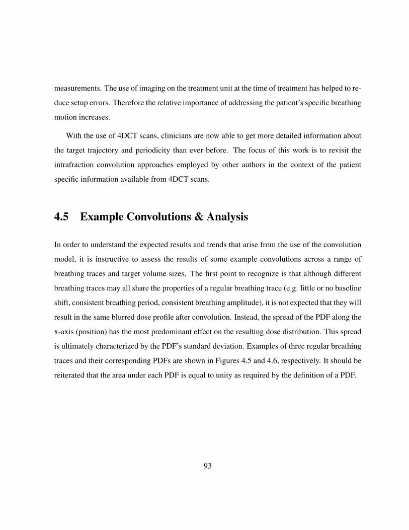
measurements. The use of imaging on the treatment unit at the time of treatment has helped to re-

duce setup errors. Therefore the relative importance of addressing the patient’s specific breathing

motion increases.

With the use of 4DCT scans, clinicians are now able to get more detailed information about

the target trajectory and periodicity than ever before. The focus of this work is to revisit the

intrafraction convolution approaches employed by other authors in the context of the patient

specific information available from 4DCT scans.

4.5 Example Convolutions & Analysis

In order to understand the expected results and trends that arise from the use of the convolution

model, it is instructive to assess the results of some example convolutions across a range of

breathing traces and target volume sizes. The first point to recognize is that although different

breathing traces may all share the properties of a regular breathing trace (e.g. little or no baseline

shift, consistent breathing period, consistent breathing amplitude), it is not expected that they will

result in the same blurred dose profile after convolution. Instead, the spread of the PDF along the

x-axis (position) has the most predominant effect on the resulting dose distribution. This spread

is ultimately characterized by the PDF’s standard deviation. Examples of three regular breathing

traces and their corresponding PDFs are shown in Figures 4.5 and 4.6, respectively. It should be

reiterated that the area under each PDF is equal to unity as required by the definition of a PDF.

93

Figure 4.5: Examples of regular breathing traces. Despite being different from one another, each

trace could be considered regular due to stable breathing frequency, amplitude and baseline.

94

Figure 4.6: The PDFs and PDF gradients corresponding to the regular breathing traces above.

Although each trace is regular in nature, the PDFs resulting from each trace are quite different

in terms of standard deviation. Figure A depicts the corresponding PDFs on the same axes to

contrast their shape. Figure B plots the gradients of each PDF.

95

The convolution of each of these PDFs with a static dose distribution ultimately reveals the

effect of target motion on the delivered dose distribution. Since small targets are more susceptible

to loss of dose coverage, it is important to assess the result of the convolution on a range of target

sizes. These results for the three regular traces described in this section are shown in Figure 4.7.

Figure 4.7: Examples of blurred dose distributions resulting from the convolution of the regular

breathing trace PDFs and the dose profiles corresponding to a range of target sizes. Dashed lines

are the original static profiles, solid lines are the resulting blurred distributions. The target size

is characterized by the dose profile’s full-width-half-max (FWHM). (i),(ii) and (iii) depict the

resulting blurred distributions for the PDFs with SD of 0.12 cm, 0.5 cm and 0.96 cm respectively.

96

It is clear from Figure 4.7 that as the standard deviation of a given PDF increases, so does the

amount of blurring in the resulting dose distribution. The susceptibility of small targets to large

motion is also highlighted in Figure 4.7 (iii) where both the dose coverage and maximum dose

delivered to the small target have seen a substantial drop.

The trend in the amount of blurring resulting from the convolution also holds true for irregular

breathing traces. An irregular breathing trace is typically characterized by baseline shifts, incon-

sistent breathing period and/or inconsistent breathing amplitude. As with the regular breathing

traces, a set of irregular traces are not expected to result in similar dose blurring after convolu-

tion simply based on these attributes. Again, it is seen that the spread along the x-axis (standard

deviation) of the breathing trace PDF is what best predicts the resulting blurring. Examples of

three irregular breathing traces and their corresponding PDFs are shown in Figure 4.8 and 4.9,

respectively. As with the regular breathing PDFs, the irregular PDFs are also normalized such

that the area under the curve is unity.

97

Figure 4.8: Examples of irregular breathing traces. Each trace exhibits breath-to-breath irregu-

larities in at least one of: breathing amplitude, breathing frequency or baseline location.

Figure 4.10 shows the resulting convolutions of the irregular breathing traces with the same

three target dose profiles. The clear trend of increasing blurring with increasing PDF standard

deviation is again apparent in the case of the irregular breathing traces.

98

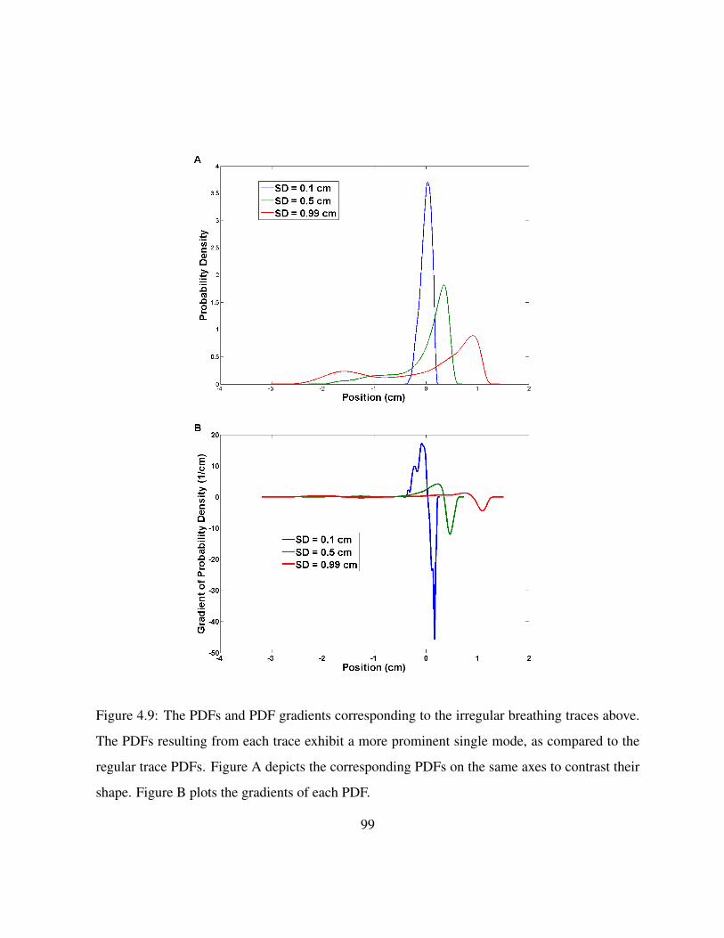
Figure 4.9: The PDFs and PDF gradients corresponding to the irregular breathing traces above.

The PDFs resulting from each trace exhibit a more prominent single mode, as compared to the

regular trace PDFs. Figure A depicts the corresponding PDFs on the same axes to contrast their

shape. Figure B plots the gradients of each PDF.

99

Figure 4.10: Examples of blurred dose distributions resulting from the convolution of the irreg-

ular breathing trace PDFs and the dose profiles corresponding to a range of target sizes. Dashed

lines are the original static profiles, solid lines are the resulting blurred distributions. The target

size is characterized by the dose profile’s full-width-half-max (FWHM). (i),(ii) and (iii) depict

the resulting blurred distributions for the PDFs with SD of 0.1 cm, 0.5 cm and 0.99 cm respec-

tively.

It is also important to note the relative asymmetry of the blurred dose profiles resulting from

the convolution with irregular breathing in Figure 4.10 (iii) and regular breathing in Figure 4.7

(iii). This asymmetry is best explained by looking at the gradient of the PDFs as suggested by

Equation 4.13. In the case of the large standard deviation PDFs for both regular and irregular

traces, we can plot the PDFs along with their derivatives, as shown in Figure 4.11.

100

Figure 4.11: A plot of a regular and an irregular breathing trace PDF with their gradients. In

these cases, the PDFs have substantial asymmetry due to the specific breathing patterns. As a

result, the PDF gradients also have large asymmetry. The large asymmetry in the PDF gradient

is what contributes to an asymmetric blurred dose profile.

101

When performing the calculation defined in Equation 4.13 it can be seen that the regions of

the ddxPDF (x) that are equal, or nearly equal, to zero will offer little or no contribution to the

resulting convolution. Correspondingly, regions of the ddxPDF (x) which are largest will make

the largest contribution to the resulting convolution. The PDF gradient highlights these regions.

In the case of Figure 4.11, a prominent asymmetry in the ddxPDF (x) can be seen. This feature

of the PDF gradient is not being balanced by any other features of ddxPDF (x) and as a result,

creates the asymmetry seen in the blurred profiles.

4.6 Summary

The convolution model has been used by many different researchers to assess the impact of

interfraction and intrafraction organ motion on the delivered dose distribution. Jiang et al. [24]

showed the model can be reformulated in terms of the static dose gradient, or equivalently, the

PDF gradient. This approach highlights the features of the inputs which have the most prominent

effect on the resulting blurred dose distribution.

The convolution model requires two inputs: a static dose distribution and a PDF describing

the target motion. In this work the static dose distribution must come from a plan generated

on an image of the patient with the target in its average position. The PDF describing target

motion is garnered from 4DCT data. Tied to these inputs are the assumptions of shift invariance

and sufficient sampling. As has been reported by other authors and investigated in this work,

the model assumptions can be met to a reasonably strong degree, providing confidence in the

modified dose predictions made by the convolution model.

The trends in target dose blurring that result from the convolution of PDFs and dose profiles

of various sizes show the impact of the PDF standard deviation and gradient of the PDF on the

102

delivered dose distribution. The asymmetric nature of gradient of the breathing trace PDFs also

determines asymmetric blurring of the dose distribution.

103

Chapter 5

Film Measurement Procedures and Results

5.1 Introduction

The convolution model of target motion described in Chapter 4 is most frequently used in the

context of predicting the effect of interfraction target motion on delivered dose distributions. This

type of work was done in the context of random setup errors for tumour sites such as prostate

[24, 115], liver [116, 117], or head and neck [118, 119]. However, this study looks to extend the

use of the convolution model to intrafraction motion. In order to have confidence that this model

can be used in the context of intrafraction motion, experimental measurements must be made to

verify the predictions made by the convolution model.

Radiochromic film is the dosimeter of choice for performing these verification measurements.

Film offers the best combination of spatial resolution, signal to noise ratio and ease of use for

this application. Additionally, film has the advantage of offering a dose measurement over a 2D

region of interest. This allows the user to extract dose profiles or perform dose map comparisons

with the dose predictions made by the treatment planning software. In this work there is also a

104

need for comparison with dose predictions made by the convolution model itself. The film mea-

surements performed for this work were taken in a dynamic anthropomorphic thorax phantom

that was programmed to perform custom breathing motions. The details of the phantom and film

measurements are given in this chapter.

5.2 Radiochromic Film Handling

The radiochromic film used in this work was Gafchromic EBT2 (International Specialty Prod-

ucts, Wayne, NJ). This film offers several advantages over traditional radiochromic film products.

Gafchromic EBT2 film requires no processing, which eliminates the need for a darkroom and the

associated equipment and chemicals. Gafchromic EBT2 also has low energy dependence and re-

acts independently of dose rate and fractionation [122].

Gafchromic EBT2 film consists of several layers of material: a base layer (175 µm), an active

layer (28 ± 3 µm), an adhesive layer (25 µm) and a laminate layer (50 µm) as shown in Figure

5.1 [122]. The film works by undergoing chemical changes in the active layer in response to the

absorbed dose. The active layer of Gafchromic EBT2 consists of diacetylene monomers oriented

in the same direction. In response to the absorbed dose, the monomers react with one another to

form polymers. The result of this reaction is a change in the optical properties of the film, which

can then be used to assess the absorbed dose.

105

Figure 5.1: A depiction of Gafchromic EBT2 film configuration as shown in the Gafchromic

EBT2 white paper published by ISP [122]. Optical density changes in the film result from poly-

merization reactions in the active layer.

Proper handling of the film includes several steps and considerations as detailed by the manu-

facturer [122], and expanded upon in the AAPM TG-55 report titled ‘Radiochromic film dosime-

try: Recommendations of AAPM Radiation Therapy Committee Task Group 55’ [123]. These

recommendations span topics regarding the handling, calibration and readout of radiochromic

film. The key recommendations made by these groups are as follows:

• The film should be exposed to the minimum possible amount of ambient light. Although

the manufacturer claims the film is stable in ambient light, the ultraviolet component of the

light can contribute to changes in optical density of the film. Andres et al. [124] showed

that a 6 hour exposure to (relatively intense) room lighting changed the optical density of

Gafchromic EBT2 by the equivalent of a 6.1 cGy dose.

• The film should be handled by touching the sides and edges of the film with careful at-

106

tention paid to avoiding leaving fingerprints or other marks in the area of the film to be

used for dose measurement. Any marks or fingerprints on the film will adversely affect the

readout of the film.

• It is important to maintain a consistent orientation of the film for readout [124]. The

monomers in the active layer are anisotropic and have a specific orientation which results

in different readout values depending on the orientation of the film on the scanner bed.

• The film must be digitized at a specific time interval after irradiation due to post-exposure

changes in the film. This is because the initial polymerization reaction takes place in

approximately 30 ms, however slow changes continue to take place over the course of

hours after exposure. Andres et al. showed that a minimum of 2 hours is required, post

exposure, for the film to stabilize [124].

• The lot number and model number of the film should always be noted so that any variation

in the manufacture of the film can be accounted for, if necessary.

• Calibration of the film should use a well-characterized, uniform radiation field.

• The calibration should be performed over the range of dose values expected to be measured

experimentally.

For this work, Gafchromic EBT2 film of the same batch (lot # A02181104) was calibrated

and handled according to the procedures laid out in AAPM TG-55 [123] and the recommenda-

tions of the manufacturer [122]. All the films were digitized with an Epson 10000XL flatbed

scanner (US Epson, Long Beach, CA) 22 hours after irradiation. This time frame was selected to

allow for the film to develop and to provide consistency in the handling procedure. Calibration

and analysis of the images was performed using the RIT v1.2 software package (Radiological

107

Imaging Technology, Inc., Colorado Springs, CO). Careful handling and digitization of the films

used for calibration and measurement allows for dose measurements near 200 cGy to be acquired

with a relative uncertainty of ±6% [125].

5.3 Radiochromic Film Calibration

Calibration of the Gafchromic EBT2 film was performed by irradiating pieces of film to a known

dose and then reading the optical density of the films using a flatbed scanner. New pieces of film

from the same batch (or sheet) can then be used experimentally and compared to the calibration

films in order to determine dose. The film calibration was performed in a ’solid water’ phantom

setup as depicted in Figure 5.2. The setup has a source-to-surface distance (SSD) of 95 cm,

source-to-axis distance (SAD) of 100 cm and a field size of 10 x 10 cm at isocentre. This setup

mimics the absolute dose calibration geometry used by the Grand River Regional Cancer Centre

(GRRCC). The LINACs at GRRCC have been calibrated such that 1 MU delivers 1 cGy to the

centre of the field under these setup conditions.

A single piece of film was cut into 13 squares with a side length of 5 cm. The films were

labeled and their orientation relative to the original full sheet of film was noted. Each piece of

film to be used for calibration was placed in the centre of the 10 x 10 cm field (at isocentre) with

5 cm of solid water on top and 10 cm of solid water below to provide back scatter material. Each

piece of film used for calibration was irradiated once with a predetermined number of monitor

units.

108

Figure 5.2: A depiction of the film calibration setup geometry. In this configuration, one monitor

unit delivers one cGy of dose to the centre of the film.

The manufacturer’s recommended analysis of the irradiated films is for a minimum of 13

dose points, including zero dose, to generate a reliable calibration curve. The dose points used

should cover the range from zero to a value at least 25% larger than the highest dose you expect

to measure with the current calibration [122]. The dose points used for this calibration were:

300, 240, 200, 160, 120, 90, 70, 50, 40, 30, 20, 10 and 0 cGy. Example calibration films scanned

together to show contrast are displayed in Figure 5.3.

109

Figure 5.3: Example calibration films after irradiation. The films are shown scanned together in

order to demonstrate the colour progression associated with increased dose delivered to the film.

In order to digitize the films, the scanner was first allowed to warm up. After warming

the scanner, the films are scanned individually and are each placed on the same area of the

scanner bed by using a template to align the film. Each film is scanned using the same settings.

The scanning resolution was set to 72 DPI to balance image noise and image resolution. After

all the films were scanned, each image was imported into the RIT software for analysis. The

calibration curve is created by first selecting a region of interest on each calibration film. The

optical density data in the region of interest is averaged to determine the optical density value

which corresponds to the given dose level. The film scanner measures the amount of transmission

of light through a film and converts this analog signal into digital values with a range between 0

and 65,535 A/D units, where 0 is no light being transmitted (most dense) and 65,535 indicates

that the light is transmitted through air (least dense). The A/D units are used in the calibration

110

software to generate the calibration cure. The graph of A/D units versus dose is then created

with each of the 13 data points plotted. The calibration curve was fitted to the data using a cubic

spline. The calibration data is shown in Figure 5.4. The doses delivered during experimental film

measurements can then be analyzed based on the calibration curve.

Figure 5.4: The calibration curve for Gafchromic EBT2 film used in this work. The curve

consists of 13 data points and a cubic spline fit with R2 = 0.9999.

111

5.4 Anthropomorphic Breathing Phantom Film Measurements

Description of the Phantom

In order to verify the delivery of the dose distribution calculated by Eclipse v10.1 TPS (Varian

Medical Systems, Inc., Palo Alto, CA) and predicted by the convolution model, Gafchromic

EBT2 film measurements were taken in an anthropomorphic breathing phantom. The CIRS Dy-

namic Thorax Phantom, Model 008 (Computerized Imaging Reference Systems, Inc., Norfolk,

VA) used for these measurements is shown in Figure 5.5. The phantom is made of epoxy ma-

terials that are radiologically equivalent to tissue in the energy range of 50 kV to 25 MV . It is

equipped with a drive unit capable of performing target motions with sub-millimeter accuracy

and reproducibility. The phantom can accommodate different dosimeters (film, MOSFET or ion

chambers) depending on its configuration. The dimensions of the thorax phantom represent the

‘average man’ [126].

Figure 5.5: A picture of the CIRS Dynamic Thorax Phantom, Model 008. This phantom was

used for all film measurements.

112

The phantom can be used in both static and dynamic modes. In the static mode, the phantom

is at rest and no target motion is used. In dynamic mode the phantom can perform many dif-

ferent motions. The phantom system comes pre-programmed with several sinusoidal ‘breathing

patterns’ to choose from. However, the phantom can also be manually programmed to replicate

custom breathing patterns with one dimensional target motion. For this work, film measure-

ments were taken in both static and dynamic modes for the verification of the delivered dose

distributions.

CT Simulation of the Phantom

A CT simulation of the static phantom was acquired at the GRRCC using a Siemens SOMATOM

Sensation Open scanner (Siemens AG Medical Solutions, Erlangen, Germany). This is a large

bore scanner capable of complete gantry rotations as fast as 0.5 s. The scanner uses a propri-

etary STRATON X-ray tube that functions with tube current in the range of 28 − 400 mA and

tube voltage of 80, 100, 120 or 140 kV . The scanner features 26, 880 detectors arranged in 40

rows and is capable of reconstructing images with isotropic voxels with side length as small as

0.33 mm [127].

The CIRS phantom was scanned using a typical departmental chest scan protocol. The chest

scan protocol used a tube voltage of 120 kV and tube current of 55 mA. The resulting dataset

is reconstructed with anisotropic voxels with axial dimensions of 0.0977 x 0.0977 cm and slice

thickness of 0.3 cm. The phantom was setup and aligned on the CT couch using the external

markers affixed to the phantom and the in room lasers for reference. Figure 5.6 is a coronal slice

at the plane of interest in the phantom CT data set used for treatment planning.

113

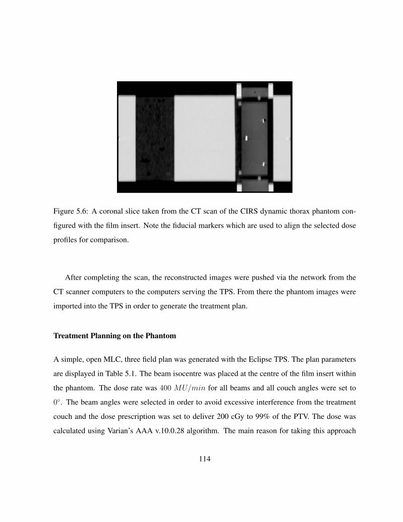
Figure 5.6: A coronal slice taken from the CT scan of the CIRS dynamic thorax phantom con-

figured with the film insert. Note the fiducial markers which are used to align the selected dose

profiles for comparison.

After completing the scan, the reconstructed images were pushed via the network from the

CT scanner computers to the computers serving the TPS. From there the phantom images were

imported into the TPS in order to generate the treatment plan.

Treatment Planning on the Phantom

A simple, open MLC, three field plan was generated with the Eclipse TPS. The plan parameters

are displayed in Table 5.1. The beam isocentre was placed at the centre of the film insert within

the phantom. The dose rate was 400 MU/min for all beams and all couch angles were set to

0◦. The beam angles were selected in order to avoid excessive interference from the treatment

couch and the dose prescription was set to deliver 200 cGy to 99% of the PTV. The dose was

calculated using Varian’s AAA v.10.0.28 algorithm. The main reason for taking this approach

114

to the treatment plan is that simple open fields result in dose profiles with the steepest dose

gradients. This makes these types of plans the most susceptible to loss of dose coverage due to

target motion. The dose profiles taken from film measurements of this plan were compared to

the dose profiles calculated by Eclipse at the same location inside the phantom.

Beam 1 Beam 2 Beam 3

Gantry Angle (deg) 315 0 45

(X,Y) Jaw settings (cm) (3.7 , 3.7) (3.2, 3.7) (3.6, 3.7)

MU 86.6 92.5 93.9

Table 5.1: A summary of the treatment plan parameters used to irradiate the phantom for static

and dynamic film measurements. The coordinate system used is the IEC convention.

In order to compare dose profiles from the TPS dose calculations to the profiles measured

on film, careful consideration must be given to geometry of the film insert. The phantom’s

film insert accepts rectangular pieces of film cut to dimensions of 13.5 x 4 cm. As can be

seen in Figure 5.6, the phantom’s film insert has pegs to allow for consistent film placement.

The pegs also serve to align both halves of the film insert, and hold them together. The film

insert also has fiducial markers placed within it to provide reference points on the CT images

for film measurement comparisons. Comparison of the measured and calculated dose profiles

was achieved by selecting a dose profile along the superior-inferior direction of the phantom

through treatment plan isocentre, in the TPS. The distance from the right edge of the film to the

selected dose profile was then recorded. After irradiating and digitizing the film, the measured

dose profile for comparison was selected by measuring the same distance from the edge of the

film, then selecting the dose profile passing through that point, parallel to the length of the film.

All dose profiles originated at the superior edge of the film.

115

5.5 Film Measurements in the Static Phantom

The film measurements taken in the static mode were used to determine confidence in the re-

peatability and accuracy of the film handling and measurement procedures. These results also

serve to verify the calculations made by the Eclipse TPS environment. In order to acquire the

static film measurements, the CIRS phantom was setup on the treatment unit using the same

configuration as at the time of CT scanning. The external markers on the phantom were aligned

with the in room lasers. After aligning the phantom with the lasers the required couch shifts were

applied, such that the treatment beam isocentre was at the centre of the film insert as planned.

The couch shifts were predetermined by the TPS by comparing the location of the isocentre at

the time of the CT simulation to the location of the beam isocentre in the treatment plan.

The dose profile resulting from a static phantom film measurement is shown in Figure 5.7.

The absolute dose profiles have good agreement with the predictions made by Eclipse. In this

case, 96.1% of the measured dose points are within 3% or 3 mm of the corresponding dose

points in the Eclipse prediction. These criteria are commonly used when assessing the level of

agreement between a measured and calculated dose plane in the context of a gamma evaluation

[128], and is similar to the recommendations of Van Dyk et al. [129] for a quality assurance

threshold. The error bars represent±6% of the absolute dose, which is the error level that can be

expected with good handling techniques as determined by Hartmann et al. [125].

116

Figure 5.7: A comparison of the dose profile calculated by the Eclipse TPS and the corresponding

dose profile measured on radiochromic film in the CIRS phantom in static mode.

Several such film measurements were performed over the course of this work. The resulting

dose profile comparisons consistently showed good agreement between film measurement and

dose calculation in Eclipse. The static dose profile measurements were an important part of

refining the measurement technique and building confidence in the measurement procedure and

results.

117

5.6 Film Measurements in the Dynamic Phantom

Film measurements were also taken with the phantom in the dynamic mode. This was achieved

by programming the one dimensional motion of the phantom insert to replicate the motion of

selected patient breathing traces. Programming the phantom to perform a custom motion based

on a recorded breathing trace requires several steps. First, the recorded trace data needs to be

manipulated and scaled such that it is geometrically centered with a maximum amplitude of 1

and minimum amplitude of -1 (arbitrary units). The manipulated trace also needs to be smoothed

to remove any fine structure from the recorded trace. The smoothing step is necessary to avoid

damaging the phantom motion hardware. The trace manipulation and smoothing was performed

in MATLAB. The next step is to reformat the trace data such that it is readable by the motion

controlling software (Motion Perfect 2.4.4, Trio Motion Technology, Freeport, PA, USA) of

the CIRS phantom. The CIRS phantom can then be connected to the computer running Motion

Perfect via the serial port. With the custom trace data loaded on the computer, the CIRS phantom

can then be made to perform the custom motion by setting it to manual motion mode and issuing

the command to start the motion. The amplitude, A, of motion performed by the phantom is

defined by the user. The scaled breathing trace will then span the range [−A,A] when performing

the custom motion.

The film measurements taken with the phantom in the dynamic setting were used to verify the

ability of the convolution model to predict the effect of intrafraction motion on the delivered dose

distribution. Several patient breathing traces were used; some with regular repetitive breathing

and others with highly irregular breathing patterns. With the film insert in place and the phantom

set to perform the custom motion, the same three field treatment plan used for the static case

was delivered to the target. The dose profiles from the films acquired in the dynamic mode were

compared to the dose profile predictions made by the convolution model. Figure 5.9 and Figure

118

5.11 present the results of two such dynamic phantom film measurements.

Figure 5.8: A) A regular breathing trace used to program the dynamic thorax phantom. C) The

PDF generated from the trace (standard deviation of 0.52 cm).

119

Figure 5.9: D) Dynamic mode dose profile measurements demonstrating the applicability of the

convolution model for intrafraction motion in the case of regular breathing traces.

120

Figure 5.10: A) An irregular breathing trace used to program the dynamic thorax phantom. C)

The PDF generated from the trace (standard deviation of 0.40 cm).

121

Figure 5.11: D) Dynamic mode dose profile measurements demonstrating the applicability of

the convolution model for intrafraction motion for irregular breathing traces.

The selected traces were used to demonstrate that the convolution model makes valid predic-

tions for a range of breathing patterns, including regular and irregular breathers. In the case of the

regular breathing pattern (Figure 5.9), 98.9% of the measured dose points passed the 3% / 3 mm

criteria, while the measurement of the irregular breathing pattern (Figure 5.11) dose distribution

passed on 98% of dose points. The obvious discrepancy between the Eclipse calculation and the

convolution model prediction (and corresponding film measurement) is the ‘blurring’ effect of

target motion. Eclipse dose not account for target motion while performing the dose calculation.

These results underscore the needs for target motion management.

122

5.7 Summary

These experimental measurements were necessary to verify the validity of the convolution model

in the context of intrafraction motion, and to assess the use of the margin recommendations made

in this work. The results show good agreement between the TPS calculations and film measure-

ments taken in the static phantom, which gives confidence in the film handling and measurement

procedures. The dynamic mode film measurements have good agreement with the predictions

made by the convolution model for both regular and irregular breathing patterns.

These experimental results indicate that under most circumstances the convolution model

makes valuable predictions regarding the effect of motion on the delivered dose distribution. The

confidence developed in the accuracy of the motion model justifies larger scale simulation and

analysis of the effect of breathing motion on the delivered dose distribution. The results of such

an analysis could be used to identify trends in the resulting dose coverage, which could then

inform intrafraction motion management strategies.

Film measurement procedures such as these could provide an effective QA procedure for

measuring dose profiles with patient specific breathing patterns measured during 4DCT scans.

This verification could be done on a plan-by-plan basis to provide clinicians confidence that

increased margins are justified and offer an effective means for compensating for target motion.

123

Chapter 6

Motion Simulation Study

6.1 Introduction

Confidence in the reliability of the convolution model for intrafraction target motion has been es-

tablished by performing radiochromic film measurements as described in Chapter 5. These static

and dynamic mode film measurements provide the basis for further analysis on the effect of tar-

get motion by analyzing the predictions of the convolution model on a larger scale. Ultimately,

one of the aims of this work is to generate margin predictions which can be used by clinicians

while making treatment planning decisions. In order to accomplish this aim, we need to analyze

the effect of target motion on the delivered dose distribution under a wide range of conditions.

Specifically we want to analyze a variety of breathing patterns and target sizes in order to estab-

lish trends that can be used to make margin recommendations. Computational simulation of the

target motion allows for the rapid data generation and analysis required to identify these trends.

The motion simulations generated in this work were performed in MATLAB using standard

MATLAB routines and custom code. As discussed in chapter 4, the convolution model requires

124

the input of a motional PDF obtained from a 4DCT scan and a static dose profile. The motional

PDFs were generated from each of 502 unique patient breathing traces. The traces used in this

work were recorded from patients undergoing clinical 4DCT scans over a four year period at

the London Health Sciences Centre. The static dose profiles were obtained by first generating

a simple treatment plan on a CIRS Dynamic Thorax phantom (described in chapter 3) in the

Eclipse treatment planning software. Static dose profiles along the appropriate directions were

then exported from the treatment plan and used in the MATLAB simulation. The results of the

simulation described in this chapter and film measurements described in chapter 5 were published

in the Journal of Applied Clinical Medical Physics [130].

6.2 MATLAB Simulation Process

The effect of motion on the delivered dose distribution as predicted by the convolution model was

simulated for each of the 502 patient breathing traces on a set of static dose profiles generated

from targets ranging from 2-10 cm in diameter. An in house MATLAB program was used to

perform the convolutions and analyze the dose coverage offered by the resulting blurred dose

profiles. The main dose coverage metric used to assess the effect of the target motion was the

D95. The D95 is defined as the minimum dose received by 95% of the target volume. This metric

is akin to a point on a dose-volume histogram (DVH) and is used to assess the quality of the dose

coverage offered by a given treatment plan. Other dose coverage metrics such as the equivalent

uniform dose andD99 were also assessed. Below is the pseudo code description of the simulation

process:

• IMPORT list of static dose profile files

• FOR EACH static dose profile file:

125

– compute dose coverage metrics of the static profile

• IMPORT list of breathing trace files

• FOR EACH breathing trace file:

– extract positional data recorded during beam-on

– compute breathing trace statistics (breathing amplitude, length of data recording)

– generate histogram of recorded breathing trace positions

– generate normalized PDF from histogram

– compute PDF statistics (standard deviation, mean, skewness, kurtosis)

– place PDF origin at the PDF mean

– perform convolution of PDF with EACH static dose profile

– compute dose coverage metrics of the blurred dose distribution

Having simulated the outcomes of target motion based on a wide variety of breathing traces

and target sizes, the data must be analyzed to identify trends and correlations that can be used to

justify margin recommendations.

6.3 PDF Statistics

It is useful to look at some descriptive statistics summarizing the breathing traces (and corre-

sponding PDFs) used in the simulation study. Figure 6.1 shows the distribution of the total time

recorded for each breathing trace. It should be noted that all traces are comprised of data recorded

over a minimum of 24.5 s with the median recording time of 77.9 s. Given that a typical breath-

ing cycle is approximately 3 s, recording the breathing trace on this time scale ensures that a

126

minimum of 8 breathing cycles are captured during the recording period. This gives time for any

breathing irregularities to manifest, which is a necessary requirement for a useful and reliable

breathing trace.

Figure 6.1: A histogram detailing the distribution of breathing trace recording times. The mini-

mum and maximum recording time were 24.5 s and 119.5 s respectively. The median recording

time was 77.9 s and the average recording time was 78.8 s.

The breathing amplitude and breathing trace standard deviation are also important parame-

ters for making margin recommendations. Figure 6.2 and Figure 6.3 display histograms of the

breathing amplitude and PDF standard deviation for all the breathing traces used. The amplitude

is determined by referencing the maximum displacement recorded by the marker block. The

standard deviation is calculated according to

s =

(1

n− 1

n∑i=1

(xi − x)2

)1/2

, (6.1)

127

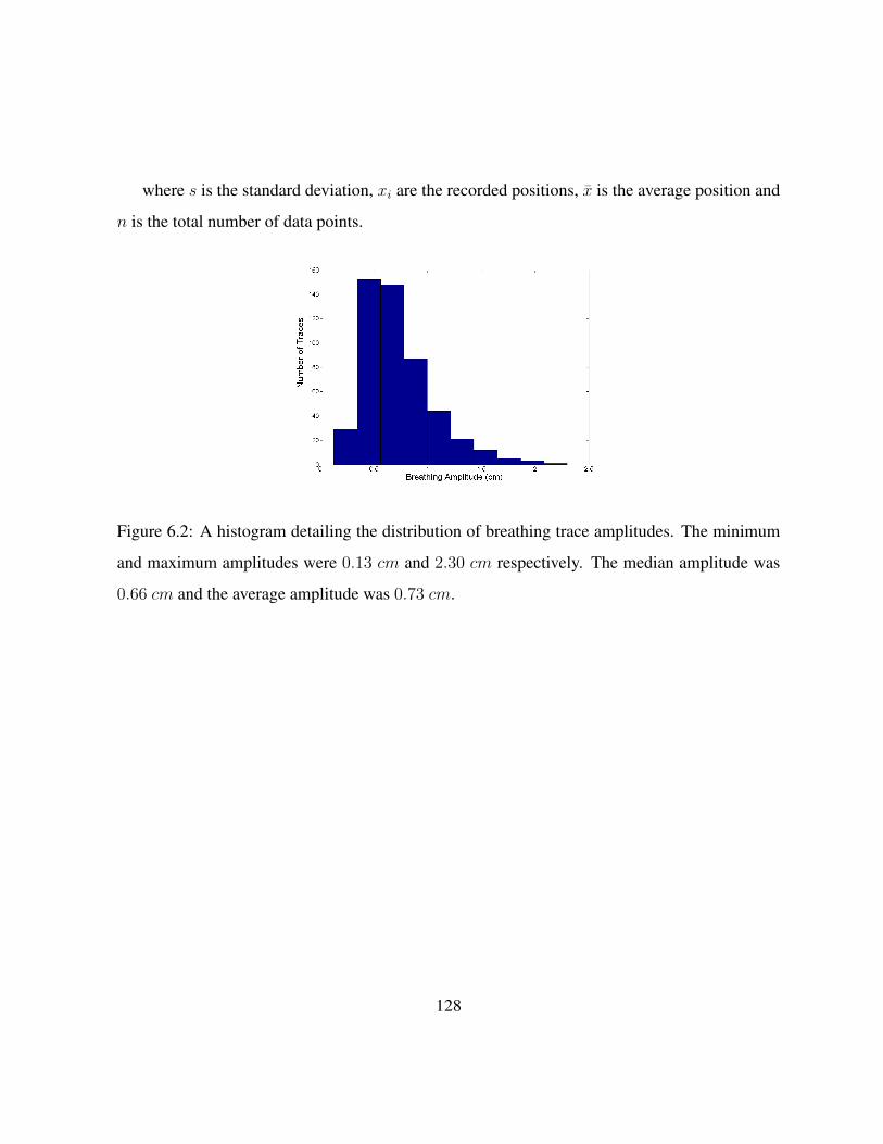
where s is the standard deviation, xi are the recorded positions, x is the average position and

n is the total number of data points.

Figure 6.2: A histogram detailing the distribution of breathing trace amplitudes. The minimum

and maximum amplitudes were 0.13 cm and 2.30 cm respectively. The median amplitude was

0.66 cm and the average amplitude was 0.73 cm.

128

Figure 6.3: A histogram detailing the distribution of breathing trace standard deviations. The

minimum and maximum standard deviations were 0.057 cm and 1.13 cm respectively. The

median standard deviation was 0.31 cm and the average standard deviation was 0.34 cm.

It should be noted that the positions (and amplitude) recorded for the breathing trace are in

fact the positions of the marker block, used as part of Varian’s RPM system, on the patient’s

chest. Although the breathing trace positions and amplitude recorded this way are not equal to

the positions or amplitude of the target motion in general, the trace can be normalized according

to the amplitude of motion determined in a 4DCT scan. Once the trace has been normalized, it is

representative of the 1D motion of the target. The breathing traces used for this simulation study

were not normalized in this manner (as would be required when applying the results of this work

clinically), however the raw trace information provides a wide range of breathing amplitudes and

trace patterns for study here.

The relationship between the PDF standard deviation and breathing amplitude is also perti-

nent. As can be seen in Figure 6.4 there is a clear correlation between the amplitude and standard

deviation. Intuitively this is the expected result; as the amplitude of the motion increases, so too

129

does the standard deviation (often interpreted as the ‘average distance from the average’ of the

data points). The slope of the best fit line is approximately 0.46 (R2 = 0.864), indicating that the

value of the standard deviation is approximately 46% of amplitude. This is similar to the result

identified by Engelsmann et al. [1]. Although the amplitude accounts for a major portion of the

standard deviation, higher order features of the PDF (such as skewness and kurtosis) also make

contributions to the PDF standard deviation.

Figure 6.4: A plot showing the relationship between the PDF standard deviation and the breathing

amplitude.

6.4 Target Volume Dose Coverage

In order to make margin selection recommendations, it is useful to know the loss of target cov-

erage which is expected on case by case basis. This simulation study revealed that the loss of

130

target D95 is predictable, based on the patient’s specific PDF standard deviation. Figure 6.5

demonstrates the relationship between the expected loss of target D95 (in terms of the ratio of the

static and blurred D95 values) and the standard deviation of the breathing pattern. These results

are in line with data presented by other authors [2, 1] regarding the predictive power of the PDF

standard deviation with regards to the target dose coverage. The D95 was used to assess dose

coverage because this metric is often used in the clinic to evaluate whether a given treatment

plan offers acceptable coverage. Other dose metrics could be used in principal, the D95 was

selected for its relevance to clinicians.

Figure 6.5: A plot of the relative D95 (blurred D95 to static D95) versus PDF standard deviation.

As the amount of motion increases, so t0o does the loss of target dose coverage.

The next assessment was to determine how much target D95 can be recovered by incremen-

tally increasing the beam width. The incremental increase in beam width was achieved by adding

the additional beam width to the center of the static dose profile, leaving the dose gradients in the

penumbral regions of the profile unchanged. This approximation allowed for rapid assessment

of the additional beam width required to recover the lost dose coverage.

131

Using MATLAB code (included in Appendix B) an iterative process was used to determine

the necessary additional beam width:

• A blurred dose profile is calculated based on a static dose profile and a given PDF.

• The relative D95 of blurred profile is calculated.

• If the relative D95 is less than 1, the width of the original static dose profile is increased (as

described above). If the relative dose profile is greater than or equal to 1, then the iterative

process stops.

• The blurred dose profile is re-calculated based on the wider static dose profile and the same

PDF.

• The relative D95 of the new blurred profile is calculated and the process repeats.

Once the iterative process has stopped, the additional beam width required to recover the

lost D95 is recorded. Shown in Figure 6.6 is a plot of the additional beam width required to

completely recover lost D95 due to dose blurring caused by target motion. The fit equation

y = 18.582x2 + 2.234x describes the data set well (R2 = 0.984).

132

Figure 6.6: A plot of the additional beam width required in the direction of motion to compensate

for loss of target D95 vs. PDF standard deviation. The additional beam width should be applied

in the direction of motion.

For example, suppose a given patient presented with a breathing trace whose PDF has a stan-

dard deviation of 0.4 cm. After referencing Figure 6.6 or using the fit equation, it is determined

that an additional 3.9 mm of beam width is required to compensate for the target motion.

6.5 Effect of Target Size

It is necessary to consider the role of target size when trying to compensate for motion and deliver

a specific D95 to the target. As the size of the target along the direction of motion increases, so

133

does the width of the dose profile (defined as the full-width-half-max [FWHM] of the profile)

required to adequately cover the target. As the FWHM of the dose profile increases, the relative

contribution of the penumbral region of the profile to the overall dose profile, decreases. Since the

penumbral region of the profile is most predominantly affected by the convolution (compared to

the central region of the profile), smaller targets will be more susceptible to loss of dose coverage

due to motion as compared to larger targets.

In order to assess this effect, the relative D95 data resulting from the convolution of each

breathing trace was analyzed over a range of target sizes. The results of this simulation study

are summarized in Figure 6.7. As the FHWM of the various profiles increases, the given profile

becomes less sensitive to motion in terms of loss of D95. For example, the target profile with

a FHWM of 2.6 cm loses approximately 7% of its original D95 when faced with target motion

of 0.4 cm standard deviation. The same level of motion causes a loss of approximately 1.5%

of the original D95 to a target profile with a FHWM of 5.1 cm. As the target FWHM increases

beyond 5.1 cm, the changes in sensitivity to motion become small. This is due to the smaller

relative contribution of the penumbral regions to wider profiles. As a result, the D95 data for

targets with FWHM greater than 5.1 cm begins to overlap with the data for the 5.1 cm target and

was therefore omitted from Figure 6.7.

134

Figure 6.7: A plot of relative D95 versus PDF standard deviation for multiple target sizes. The

sensitivity to coverage loss due to motion decreases with increasing target size. The change in

sensitivity becomes small as the FWHM of the increases beyond 5.1 cm.

The iterative process described in the previous section was extended to static dose profiles

with initial FWHM values ranging from 2.6 cm to 10.1 cm. Shown in Figure 6.8 is a plot of

the additional beam width required vs. PDF standard deviation for a range of initial static dose

profile FWHM values.

135

Figure 6.8: A plot of the additional beam width required in the direction of motion to compensate

for loss of target D95 vs. PDF standard deviation. The additional beam width should be applied

in the direction of motion. This plot includes the trends for several initial static dose profile

FWHM values

6.6 Treatment Margin Recommendations

Treatment margin recommendations can be made by using the simulation results discussed above.

The margin required to maintain the planned target D95 in the presence of breathing motion with

a given standard deviation can be calculated by using fit equations from the data presented above.

The fit equations for each of the FWHM values tested are included in Table 6.1 below, where

ABW is the additional beam width required and s is the standard deviation of the PDF describing

the motion.

136

Profile FWHM (cm) Fit equation of ABW data R2 of fit

2.6 ABW = 20.734s2 + 3.282s 0.9754

3.1 ABW = 19.098s2 + 3.574s 0.981

3.6 ABW = 18.582s2 + 2.234s 0.984

4.1 ABW = 18.84s2 + 1.003s 0.9819

4.6 ABW = 16.832s2 + 2.051s 0.9835

5.1 ABW = 16.561s2 + 1.537s 0.9849

5.6 ABW = 16.551s2 + 1.201s 0.9836

6.1 ABW = 16.213s2 + 1.353s 0.9856

7.1 ABW = 15.438s2 + 1.427s 0.9863

9.1 ABW = 13.531s2 + 1.977s 0.9894

10.1 ABW = 13.829s2 + 0.5121s 0.985

Table 6.1: A summary of equations describing the additional beam width (ABW) per unit stan-

dard deviation (s) for various target sizes.

A table of margin recommendations spanning a range of target sizes and target motions can

be generated using these equations. These margin recommendations are presented in Table 6.2

below.

137

PDF Standard Deviation (cm)

Dos

ePr

ofile

FWH

M(c

m)

0.1 0.2 0.3 0.4 0.5 0.6 0.7 0.8

2.6 0.5 (mm) 1.5 2.9 4.6 6.8 9.4 12.5 15.9

3.1 0.5 1.5 2.8 4.5 6.6 9.0 11.9 15.1

3.6 0.4 1.2 2.3 3.9 5.8 8.0 10.7 13.7

4.1 0.4 1.0 2.0 3.4 5.2 7.4 9.9 12.9

4.6 0.4 1.1 2.1 3.5 5.2 7.3 9.7 12.4

5.1 0.3 0.9 1.8 3.1 4.7 6.7 8.9 11.5

5.6 0.3 0.9 1.8 3.1 4.7 6.7 8.9 11.6

6.1 0.3 0.9 1.9 3.1 4.7 6.7 8.9 11.6

7.1 0.3 0.9 1.8 3.0 4.6 6.4 8.6 11.0

9.1 0.3 0.9 1.8 3.0 4.4 6.1 8.0 10.2

10.1 0.2 0.7 1.4 2.4 3.7 5.3 7.1 9.3

Table 6.2: Summary of the recommended additional margin required (mm) to compensate for a

loss of targetD95 due to target motion. As the FWHM of the dose profiles increases, the required

margins decrease.

6.7 Motion Simulation with Clinical Plans

Three clinical treatment plans were also selected for motion simulation: a three field, a four field

and a volumetric modulated arc therapy (VMAT) plan, all of which were used to treat patients

at GRRCC. The dose profiles from these plans were convolved with the same set of breathing

traces used in the phantom plan simulation. The clinical dose profiles and target definitions that

were originally used in these plans were kept the same for the purposes of this simulation. The

138

resulting loss of target coverage in the respective PTVs was recorded in order to assess the effect

of motion in clinically relevant situations.

The result of the target motion simulation on the clinical plans reinforces the notion that the

proper margin selection is an effective tool in compensating for target motion. After including

the modeled effect of target motion, the dose coverage still remained high for the majority of

breathing patterns. As shown in Figure 6.9 it is only after the target motion becomes large (PDF

standard deviation greater than 0.4 cm) that margins beyond what are typically applied should

be considered in order to maintain target D95.

139

Figure 6.9: A plot of the relative D95 versus the PDF standard deviation for three clinical plans

with the phantom data for comparison. The clinical plans with typical margins selected are robust

in the face of target motion up to a PDF standard deviation of approximately 0.4 cm. For target

motion beyond this level, additional margins would be required to maintain target D95.

The clinical plans show less susceptibility to motion for two main reasons: large target size

( 5 cm FWHM) and softer dose gradients as compared to the dose profile from the phantom

treatment plan. Since the dose gradients play an important role in the loss of coverage, it is

instructive to look at the width of the penumbra in the dose profiles near the beam edge of these

plans. In the cases of the clinical three field and VMAT plans, the 80%-20% penumbra was

measured at 14 mm (Figures 6.10 & 6.11). In the case of the four field plan, the penumbra of

140

the dose profile was 9 mm (Figure 6.12). In each case the dose gradient was less steep than

in the phantom plan, which had a penumbra of 8 mm. The typical clinical plan (regardless of

technique) will have dose gradients which are softer than those seen in the simple three field

phantom plans. As a result, the margin recommendations generated from the phantom plans can

be seen as a worst case scenario, and any plan with softer dose gradients will be sufficiently

compensated for by using the same margins.

141

Figure 6.10: An image through the isocentre of the clinical three field treatment plan. The inset

dose profile was used as the basis of the simulations of target motion in the case of the three field

plan. The dose profile runs from superior to inferior through the center of the treatment volume

along the vertical line indicated.

142

Figure 6.11: An image through the isocentre of the clinical VMAT treatment plan. This plan was

comprised of two arcs. The inset dose profile was used as the basis of the simulations of target

motion in the case of the VMAT plan. The dose profile runs from superior to inferior through the

center of the treatment volume along the vertical line indicated.

143

Figure 6.12: An image through the isocentre of the clinical four field treatment plan. The inset

dose profile was used as the basis of the simulations of target motion in the case of the four field

plan. The dose profile runs from superior to inferior through the center of the treatment volume

along the vertical line indicated.

Since the size of the target plays an important role in the loss of D95, it is important to

consider the width of the dose profiles in these plans. The FWHM for the clinical three field,

144

four field and VMAT plans were measured at 8.5 cm, 11.1 cm and 12.8 cm respectively. The

same trend that was identified with the study of target size can be seen in these three clinical

plans as well. However, the variation in dose gradients also plays a role in the clinical results.

The results of the phantom study are generated with very steep dose gradients resulting from

a simple three field plan with overlapping beam edges. In practice, these phantom plan dose

gradients will be as sharp as, or sharper, than what can be achieved in a clinical situation. As a

result the margin recommendations of the phantom plan can be taken as a worst case scenario,

and can be safely applied to a clinical plan which has equivalent or softer dose gradients.

The analysis of the clinical treatment plans reveals that they are rather robust in the face of

target motion. Figure 6.9 displays the loss of target D95 versus the PDF standard deviation and

also includes the phantom results of the 4.1 cm FWHM target for comparison. Images of the

dose distributions and the associated dose profiles are displayed in Figures 6.10-6.12.

The clinical plans lose very littleD95 for target motions which have a PDF standard deviation

below 0.4 cm. It is only after the PDF standard deviation is larger than approximately 0.4 cm

that the loss of target D95 becomes appreciable. This highlights the effectiveness of selecting

appropriate margins to compensate for target motion.

6.8 Example Margin Selection

Having determined recommended field margins shown in Table 6.2, it was instructive to re-

examine the dynamic phantom dose profiles measured for a small target volume and extreme

standard deviation (characteristic of a stereotactic radiosurgery case with large, irregular tumor

motion). A treatment plan for a small target (2.6 cm FWHM dose profile) was first generated

in Eclipse. The static dose profile was extracted from the treatment plan and convolved with a

145

breathing trace PDF with a large standard deviation (0.8 cm) to assess the impact of target motion

on dose coverage. A new plan was then generated by adding the appropriate margin from Table

6.2 to the small target (16 mm). The phantom was programmed to replicate the motion recorded

in by the breathing trace and the new plan was then delivered to the phantom in motion. The dose

coverage offered by the new plan under motion was then compared to the original static plan in

order to validate the use of Table 6.2 for margin selection recommendations.

The results of this validation measurement are depicted in Figure 6.13 and summarized in

Table 6.3. The D95 of the target PTV increases from 75.8% of the original D95 without motion

compensation to 99.1% with motion compensation. In this case, the additional margin would

play an important role in ensuring an adequate dose is delivered to the treatment volume in the

presence of target motion. It should also be noted that by expanding the margins in this treatment

plan, it is possible that adjacent OARs could receive an increased dose. By using the margin

recommendations in Table 6.2 a clinician would be able to assess the impact of the expanded

margin on OARs at the treatment planning stage.

146

Figure 6.13: A plot of dose profiles demonstrating the margin recommendations provided in this

work. The original static profile is taken from Eclipse, then convolved with the PDF. The original

static plan loses dose coverage due to the target motion. When the margin recommendation from

Table 6.2 is included in the plan, the target dose coverage is largely recovered when the treatment

is delivered in the presence of the same target motion.

147

Original Static

Profile (Eclipse)

Original Profile with Motion

(Eclipse, convolved)

Profile with Added Margin &

Motion (film measurement)

D95 (cGy) 189.9 143.9 188.2

Relative D95 (%) 100 75.8 99.1

Table 6.3: Summary of the results of the margin selection example to demonstrate use of the

margin recommendations presented in this work. The D95 of the PTV is largely recovered by

including the margin recommended in Table 6.2.

For this type of situation the increase in field dimensions could compromise the dose to

adjacent organs as seen in a treatment plan with adjusted margins. A clinical decision to use

a different treatment technique, instead of simply increasing the margins, could be guided by

the treatment plan with extended margins. By assessing the treatment plan with the extended

margins in place, the clinician has the ability to compare other treatment options, to a treatment

plan with margins that will compensate for target motion.

6.9 Comparison of Margin Recipes

Since Leong [22] proposed the idea of incorporating target motion into dose calculations via the

convolution model, other authors have also assessed how the blurred dose coverage depends on

the model parameters. The works of Engelsmann et al. [1], Richter et al. [2] and van Herk

et al. [13] also identified the standard deviation of the motional PDF to be a key predictor of

changes to dose coverage. Although each group used the standard deviation to make margin

recommendations, the dose coverage metrics used as the basis for comparison are different in

each case. The differences in margin recommendations made in this work and as compared

to the above cited authors offers an interesting perspective on the trade-offs and weighting of

148

outcomes that must be considered clinically when applying treatment margins to accommodate

for target motion.

6.9.1 Comparison with Engelsmann et al.

The approach detailed by Englesmann et al. [1] looks to assess how the position of the 95%

isodose line is displaced as a result of the dose profile blurring predicted by the convolution

model. In a 1D dose profile, the 95% isodose line corresponds to the point where the dose is

95% of the maximum profile dose. The location of the 95% isodose line relative to the target

PTV is used clinically to assess the quality of dose coverage offered by a give treatment plan.

By offering margin recommendations that look to preserve the location of the 95% isodose line,

the authors are looking to ensure that the abosorbed dose received by the tissue at the border of

the target volume location remains at planned level. This is in contrast to the D95 used in this

thesis (defined as the minimum dose received by 95% of the target volume), which summarizes

the dose coverage to the entire target volume. By making margin recommendations that look to

preserve the target D95, we look to ensure that the 95% of the target volume receives at least the

same dose as originally planned, after considering target motion.

A major difference in the approach Englesmann et al. used to generate the margin recom-

mendations lies in the static dose profiles used as the input to the convolution model. The authors

used an analytical expression based on the sum of Error Functions (Equation 6.2) as an approxi-

mation of a one sided dose profile only.

D(x) =ω1erf( x

b1) + ω2erf( x

b2)

2• 100% (6.2)

In this context the 0% dose is located at x = −∞, 50% dose at x = 0 and 100% dose at

x = ∞ [1]. It should be noted that the integral dose of this profile is infinite, and as such the

149

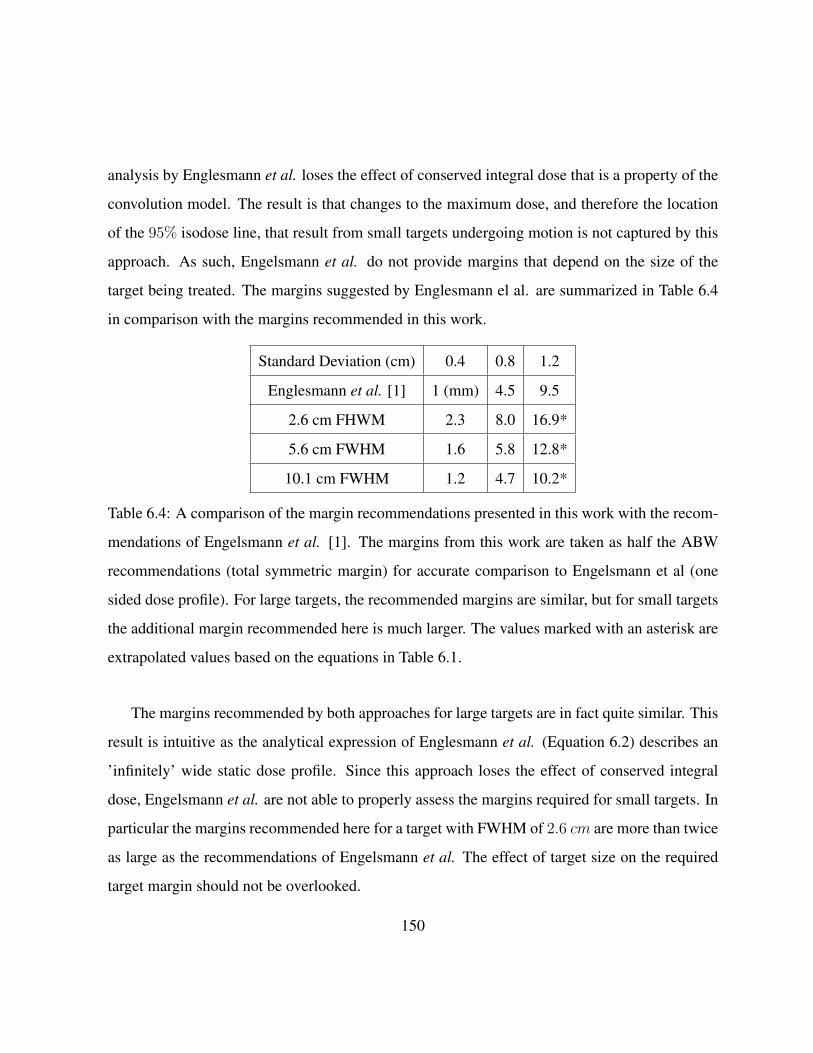
analysis by Englesmann et al. loses the effect of conserved integral dose that is a property of the

convolution model. The result is that changes to the maximum dose, and therefore the location

of the 95% isodose line, that result from small targets undergoing motion is not captured by this

approach. As such, Engelsmann et al. do not provide margins that depend on the size of the

target being treated. The margins suggested by Englesmann el al. are summarized in Table 6.4

in comparison with the margins recommended in this work.

Standard Deviation (cm) 0.4 0.8 1.2

Englesmann et al. [1] 1 (mm) 4.5 9.5

2.6 cm FHWM 2.3 8.0 16.9*

5.6 cm FWHM 1.6 5.8 12.8*

10.1 cm FWHM 1.2 4.7 10.2*

Table 6.4: A comparison of the margin recommendations presented in this work with the recom-

mendations of Engelsmann et al. [1]. The margins from this work are taken as half the ABW

recommendations (total symmetric margin) for accurate comparison to Engelsmann et al (one

sided dose profile). For large targets, the recommended margins are similar, but for small targets

the additional margin recommended here is much larger. The values marked with an asterisk are

extrapolated values based on the equations in Table 6.1.

The margins recommended by both approaches for large targets are in fact quite similar. This

result is intuitive as the analytical expression of Englesmann et al. (Equation 6.2) describes an

’infinitely’ wide static dose profile. Since this approach loses the effect of conserved integral

dose, Engelsmann et al. are not able to properly assess the margins required for small targets. In

particular the margins recommended here for a target with FWHM of 2.6 cm are more than twice

as large as the recommendations of Engelsmann et al. The effect of target size on the required

target margin should not be overlooked.

150

6.9.2 Comparison with Richter et al.

Richter et al. [2] also used the standard deviation of the motional PDF as an important predictor

in loss of dose coverage. The margins recommended by Richter et al. aim to preserve the

absorbed dose at the border of the target volume. The approach taken by the authors was to

compensate for target motion by both increasing target margin, and increasing the dose delivered

to the target. They assessed the additional margin required while also delivering 105%, 125%,

and 150% of the originally prescribed dose. Since increasing the dose delivered to the target also

compensates for the dose spillage resulting from the blurring caused by target motion, the effect

of increasing the dose to the target is to reduce the additional margin required to maintain the

dose to the edge of the target volume.

The margin recommendations from Richter et al. are summarized with comparison to this

work in Table 6.5. It can be seen in the table that the margin recommendations are similar for

medium sized targets in this case. The approach of increasing the prescribed dose allows for

smaller margins to offer the same level of dose coverage.

151

Standard Deviation (cm) 0.1 0.2 0.3 0.4 0.5 0.6 0.7

P105 0.3 (mm) 0.9 1.6 2.6 3.8 5.2 6.9

P125 0.4 0.9 1.5 2.2 3.0 4.0 5.0

P150 0.3 0.5 0.8 1.2 1.5 1.9 2.2

2.6 cm FHWM 0.5 1.5 2.9 4.6 6.8 9.4 12.5

5.6 cm FWHM 0.3 0.9 1.8 3.1 4.7 6.7 8.9

10.1 cm FWHM 0.2 0.7 1.4 2.4 3.7 5.3 7.1

Table 6.5: A comparison of the margin recommendations presented in this work (profile FWHM

specified) with the recommendations of Richter et al. [2] using different prescribed doses (P105,

P125, P150). The values for the recommended margins from Richter et al. were calculated using

the formulas given in the paper. Although Richter et al. do not specify the size of the target used

to generate this data, the recommendations from both approaches are similar for medium sized

targets.

By increasing the prescribed dose, the authors effectively increase the integral dose in the

static plan. This way, the dose spillage that results from the blurring due to target motion is

partially compensated for without increasing the target margin. The potential drawback of this

approach is the large increase in dose to surrounding healthy tissue that results from the increased

dose prescribed to the target. In many cases the dose prescribed to the target volume is limited by

the dose that will also be imparted to surrounding healthy tissues. As a result, it may not always

be safe to drastically increase the prescribed dose to a target volume in order to compensate for

target motion.

152

6.9.3 Comparison with van Herk et al.

In comparison with the approach detailed by van Herk et al [13], we can see that the margin

recommendations presented here are similar for some situations. Although the van Herk formula

makes no accounting for target size, we can compare the margin recommendations based on the

van Herk et al. ‘linear approximation of the random component for 95% dose coverage’. This

is a simple formula which approximates the margin required to compensate for target motion as

‘0.7σ’ where σ is the standard deviation of the motion. The approach of van Herk et al. seeks the

margin that results in 95% of the prescribed dose covering the target for 90% of patients. These

results are presented in Table 6.6.

Standard Deviation (cm) 0.1 0.2 0.3 0.4 0.5 0.6 0.7 0.8

van Herk Approximation 0.7 (mm) 1.4 2.1 2.8 3.5 4.2* 4.9* 5.6*

2.6 cm FHWM 0.5 1.5 2.9 4.6 6.8 9.4 12.5 15.9

5.6 cm FWHM 0.3 0.9 1.8 3.1 4.7 6.7 8.9 11.6

10.1 cm FWHM 0.2 0.7 1.4 2.4 3.7 5.3 7.1 9.30

Table 6.6: A comparison of the margin recommendations presented in this work in comparison

with the commonly used van Herk recommendations. For small targets, the recommended mar-

gins are similar, but for larger targets D95 can be maintained with less additional margin than

suggested by van Herk et al. Since van Herk et al. only claim accurate approximation of the

formula used up to a standard deviation of 0.5 cm, the values marked with an asterisk are noted

as an extrapolation.

For small targets, the margin recommendations are similar. For larger targets, the results

computed in this study suggest less additional margin is required. The differences in margin

recommendations likely arise due to differences in the approach to the problem. The approach of

153

van Herk et al. is to find margins that satisfy the majority of the population of patients studied.

However if a patient specific approach to margin selection is taken, there is opportunity for

reduced target margin for patients with larger sized targets. This can be seen in the comparison

table above where patients with small target motion (PDFSD < 0.4 cm) have smaller margin

recommendations from this work as compared to van Herk et al.

6.10 Summary

Target motion was simulated for a wide range of breathing traces and target sizes in order to

determine the loss of target dose coverage. Statistics describing the range of breathing traces

were presented. It was shown that breathing trace amplitudes in this large data set ranged from

0.13 to 2.30 cm with an average amplitude of 0.73 cm. The standard deviations of the PDFs in

the data set ranged from 0.057 to 1.13 cm with an average standard deviation of 0.34 cm.

A quadratic function used to describe the loss of target dose coverage in terms of the standard

deviation of the PDF describing the motion of the target was found to correlate strongly with the

data set (R2 = 0.9821). The size of the target along the direction of motion was also found to

influence the amount of coverage being lost, with larger targets being less susceptible to loss of

dose coverage due to motion. The recovery of target dose coverage was also found to correlate

with the PDF standard deviation, and these two trends were used to generate margin recommen-

dations. A table of margin recommendations based on the PDF standard deviation and target size

was presented in Table 6.2. These margins can be applied in a clinical situation to compensate

for the reduction of the target’s D95 due to intrafraction motion.

An example application of the use of the methodology and margin recommendation table

was presented for a small target and extreme motion. This example demonstrates how the table

154

can be used to ensure adequate dose coverage of the target volume. The influence of the studied

motions on a set of clinical treatment plans was also assessed. This assessment demonstrated the

interplay between target size, dose gradient and standard deviation of the target motion.

Finally the margins recommended in this thesis were compared with published recommenda-

tions from other authors who also took advantage of the convolution model to assess the impact

of target motion on target dose coverage. The margins presented here are comparable to those

presented by other authors under some circumstances, however the inclusion of dependence on

target size presented in this thesis offers opportunity for smaller margins for some patients, as

compared to the other recommendations.

155

Chapter 7

Convolution Model Sensitivity Analysis

7.1 Introduction

In this thesis a convolution technique has been applied to determine the impact of intrafraction

lung motion on absorbed dose. As shown previously, a patient specific lung PDF was derived

from 4DCT data, and the gradient of the PDF was convolved with the static dose profile to obtain

a blurred or motion-impacted dose gradient along the superior-inferior direction. The blurred

dose gradient was then integrated along the superior-inferior direction to obtain the blurred dose

profile. This technique was developed in Chapter 4 using Equation 4.8, expanded with clinical

examples in Section 4.5, and demonstrated graphically in Figures 4.7 to 4.11. Using a dynamic,

tissue equivalent phantom programmed for clinical breathing patterns and radiochromic film for

dose measurement, the convolution technique described above was validated experimentally and

the results were summarized in Chapter 5.

In Chapter 6, breathing patterns from 502 patients were used to simulate the effect of in-

trafraction motion on static dose profiles obtained from a standard treatment plan designed to

156

cover targets ranging from 2-10 cm in diameter. D95 was selected as the metric for comparing

static and motion-impacted dose profiles based on clinical importance and the relative D95 was

defined as the ratio of the blurred D95 to the static D95. After analysis it was determined that rel-

ative D95 has a quadratic dependence on the standard deviation of the static dose profile and this

is shown in Figures 6.5 and 6.7 and Table 6.1. A program was written in MATLAB to calculate

the additional beam width (ABW applied to the static dose profile) that is required to restore the

high dose region impacted by lung motion. Table 6.2 shows ABW as a function of the standard

deviation of the PDF and also the FWHM of the static dose profile.

In addition to the conformal treatment plan, a 3-field, 4-field and a VMAT plan were also

analyzed with the 502 patient breathing patterns to assess impact on relative D95 and the validity

of recommended margins in Table 6.2. The results were shown in Figure 6.9 and the conclu-

sion was that Table 6.2 is valid for conformal and more complex planning techniques including

multiple beams and arcs.

In Section 6.8, the margin recommendations were tested experimentally using a treatment

plan with a single beam of FWHM = 2.6 cm and the dynamic lung phantom programmed for a

lung PDF with SD = 0.8 cm. These parameters were chosen to simulate a Stereotactic Radiation

Surgery (SRS) treatment and to test the extreme margin recommendations from Table 6.2. The

results from Figure 6.13 show that D95 is restored with the recommended margins at the expense

of lower dose spillage adjacent to the target due to a wider field. This effect is shown in Figure

7.1. The intersection points of the blurred dose profiles (with and without ABW) and the static

dose profile are highlighted in the figure with ovals.

157

Figure 7.1: The D95 is restored with the additional beam width, however it comes at the expense

of lower dose spillage adjacent to the target. The intersection points of the blurred dose profiles

(with and without ABW) and the static dose profile are highlighted in the figure with ovals.

158

7.2 Factors Determining the Blurred Dose Gradient

The motivation for breaking down the convolution integral as described by Equation 4.8 is a

fundamental understanding of the factors contributing to the blurred or motion-impacted dose.

Furthermore, the selection of a principal direction of motion (the superior-inferior direction in

this analysis) provides flexibility to construct the most relevant lung PDF and to make margin

adjustments tailored to a patients breathing. As shown in Figures 4.7, 4.10, 4.11, and 6.13, the

convolution-derived, blurred dose profile depends on the following parameters:

• the shape and symmetry of the PDF along r

• the standard deviation of the PDF

• the slopes of the leading and trailing edges of the static dose profile

• the FWHM and the shape of the plateau region of the static dose profile

In this chapter an analytical model is developed to explain how each of these parameters

contributes to the blurred dose profile. In general and as shown in Figure 7.2, the leading and

trailing edges of the blurred dose profile have a lower slope than the leading and trailing edges

of the static dose profile, as a result of the convolution. For field sizes < 5 cm, the peak height

of the blurred dose profile falls below that of the static dose profile in order to conserve integral

dose (also referred to as imparted energy, [4]).

159

Figure 7.2: The D95 is restored with the addition beam width, however it comes at the expense

of lower dose spillage adjacent to the target. The intersection points of the blurred dose profiles

(with and without ABW) and the static dose profile are highlighted in the figure with ovals.

This is a consequence of the convolution theorem, which, applied to Equation 4.1 yields

∫Db(~r)dr =

∫D0(r)⊗ PDF (r)dr =

[∫D0(r)dr

]•[∫

PDF (r)dr

]. (7.1)

In this study the PDFs were normalized (i.e.∫PDF(r)dr = 1) and Equation 7.1 reduces to

160

∫Db(r)dr =

∫D0(r)dr. (7.2)

In Figure 7.2 the intersection points of the blurred and static dose profiles are identified with

ovals and their projections on the r axis are shown as −r∗ and r∗ relative to the static profile

centered at the origin. These points are used to identify regions of under and overdose for the

blurred profile relative to the static profile.

For the static dose profile,

∫ ∞−∞

D0(r)dr =

∫ −r∗−∞

D0(r)dr +

∫ r∗

−r∗D0(r)dr +

∫ ∞r∗

D0(r)dr (7.3)

and similarly for the blurred dose profile,

∫ ∞−∞

Db(r)dr =

∫ −r∗−∞

Db(r)dr +

∫ r∗

−r∗Db(r)dr +

∫ ∞r∗

Db(r)dr. (7.4)

Using Equation 7.2 and subtracting components from Equations 7.3 and 7.4,

∫ r∗

−r∗D0(r)−Db(r)dr =

∫ −r∗−∞

Db(r)−D0(r)dr +

∫ ∞r∗

Db(r)−D0(r)dr (7.5)

In words, Equation 7.5 states that the region of dose deficit shown in Figure 7.2 is equal to

the sum of the regions of dose spillage arising from the convolution of the static dose profile with

the PDF.

It is important to note that by adding additional margins to the static dose profile to recover

the dose deficit arising from lung motion (per Table 6.2), the dose spillage regions will also

expand. This means that the impact on the DVH for OARs adjacent to the target volume must be

assessed carefully along with the PTV coverage as part of using this methodology.

161

7.3 Analytical Modeling Using Gaussian PDF Functions

Since the parameters contributing to the blurred dose gradient described in the previous section

are highly patient and treatment plan specific, it is not practical to derive a comprehensive sensi-

tivity model that applies to all cases. By employing a simpler lung PDF than observed clinically,

however, it is possible to provide an analytical sensitivity analysis that explains the basic physics.

Jiang et al. [24] used a Gaussian PDF to describe interfraction prostate motion and previously

showed the equivalence of deriving the blurred dose gradient from the convolution of a static

dose profile with the gradient of a Gaussian PDF or from the convolution of the gradient of the

static dose profile with a Gaussian PDF. This is shown in Figures 7.3 and 7.4 for PDF standard

deviations ranging from 0.2 cm to 0.8 cm.

162

Figure 7.3: An example of Gaussian blurring applied to gradient of a static dose profile as de-

scribed by Jiang et al. [24]. The standard deviation of the Gaussian PDF ranges from 0.2 to 0.8

cm.

163

Figure 7.4: An example of blurring a static dose profile with the gradient of a Gaussian PDF as

described by Jiang et al. [24]. The standard deviation of the Gaussian PDF ranges from 0.2 to

0.8 cm.

Due to the symmetry of both the static dose profile and the gradient of the Gaussian PDF in

164

this example (Figure 7.4), the blurred dose gradient is also symmetric along with the resulting

blurred dose profiles.

From the analysis in Chapters 4 and 6 and preceding discussion, it is clear that the biggest

impact on the static dose profile will occur for narrow beam profiles (FWHM < 5 cm) and large

PDF standard deviations (> 4 mm). The following analysis provides a quantitative explanation

for this effect using separate Gaussian functions to describe the dose profile and PDF.

A normalized uni-variate Gaussian function (centered on the origin) is described by

G(r) =1

σ√

2πe−

12( rσ)2 . (7.6)

The first partial derivative is given by

∂

∂rG(r) =

−rσ2G(r) =

−rσ3√

2πe−

12( rσ)2 , (7.7)

and the second partial derivative is given by

∂2

∂r2G(r) =

−σ2 + r2

σ4G(r) =

−σ2 + r2

σ5√

2πe−

12( rσ)2 , (7.8)

which will be zero when r = ±σ.

When r = ±σ the slope of G(r) will be maximized (designated by MS)

GMS =

[∂

∂rG(r)

]r=σ

= − e−12

σ2√

2π. (7.9)

When r = 0, G(r) will be have maximum peak height (designated by PH)

GPH = G(0) =1

σ√

2π. (7.10)

165

The convolution of two normalized Gaussian functions

G1(r) =1

σ1√

2πe− 1

2( rσ1

)2 (7.11)

and

G2(r) =1

σ2√

2πe− 1

2( rσ2

)2 (7.12)

is given by

G3(r) = G1(r)⊗G2(r) =1

σ3√

2πe− 1

2( rσ3

)2, (7.13)

where

σ3 =√σ21 + σ2

2. (7.14)

Using Equations 7.6 to 7.14, let G1(r) represent the normalized lung PDF obtained from

4DCT and G2(r) represent the dose profile along the direction of relevant lung motion, r. Be-

cause G2(r) was defined as a normalized Gaussian, it needs to be scaled by σ2√

2π so that the

height of the dose profile is unity (i.e. 100% or 1.0). This axis can also be scaled by absolute

dose with units of Gy. The net result is a scaled convolution Gaussian described by

G4(r) = σ2√

2πG3(r), (7.15)

and the maximum slope of G4(r) when r = σ3 is given by

166

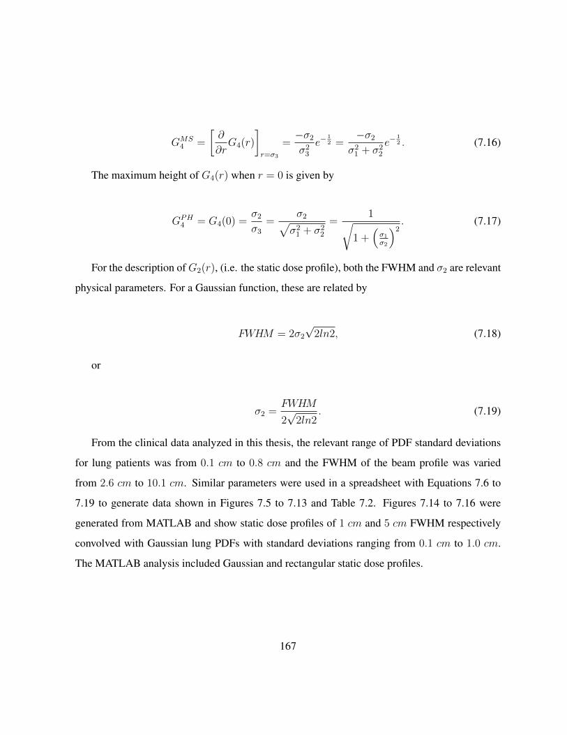
GMS4 =

[∂

∂rG4(r)

]r=σ3

=−σ2σ23

e−12 =

−σ2σ21 + σ2

2

e−12 . (7.16)

The maximum height of G4(r) when r = 0 is given by

GPH4 = G4(0) =

σ2σ3

=σ2√σ21 + σ2

2

=1√

1 +(σ1σ2

)2 . (7.17)

For the description ofG2(r), (i.e. the static dose profile), both the FWHM and σ2 are relevant

physical parameters. For a Gaussian function, these are related by

FWHM = 2σ2√

2ln2, (7.18)

or

σ2 =FWHM

2√

2ln2. (7.19)

From the clinical data analyzed in this thesis, the relevant range of PDF standard deviations

for lung patients was from 0.1 cm to 0.8 cm and the FWHM of the beam profile was varied

from 2.6 cm to 10.1 cm. Similar parameters were used in a spreadsheet with Equations 7.6 to

7.19 to generate data shown in Figures 7.5 to 7.13 and Table 7.2. Figures 7.14 to 7.16 were

generated from MATLAB and show static dose profiles of 1 cm and 5 cm FWHM respectively

convolved with Gaussian lung PDFs with standard deviations ranging from 0.1 cm to 1.0 cm.

The MATLAB analysis included Gaussian and rectangular static dose profiles.

167

7.4 Analysis of Gaussian Convolution Model

The most important results from the analysis are shown in Figures 7.5 and 7.6. Figure 7.5 shows

that the maximum height of the blurred dose profile varies as 1σ3

and Figure 7.6 shows that the

maximum slope of the blurred dose profile varies as 1σ23. The relative dependencies of both the

maximum height and maximum slope on σ1 and σ2 (or FWHM) are largely determined from

Equation 7.14 (i.e. σ23 = σ2

1 + σ22) as explained in the previous section.

168

Figure 7.5: The plot of maximum blurred dose peak height versus the standard deviation of the

blurred dose profile for several static dose profile FWHM values. The PDF standard deviation

ranges from 0.1 cm to 1.0 cm. As the combined standard deviation (SD3) increases, the peak

height of the blurred dose profile decreases. As the FWHM of the static dose profile increases,

the sensitivity of the peak height to SD3 decreases.

169

Figure 7.6: The plot of maximum blurred dose gradient versus the standard deviation of the

blurred dose profile for several static dose profile FWHM values. The PDF standard deviation

ranges from 0.1 cm to 1.0 cm. As the combined standard deviation (SD3) increases, the maxi-

mum dose gradient of the blurred dose profile decreases. As the FWHM of the static dose profile

increases, the sensitivity of the the maximum dose gradient to SD3 decreases.

The simultaneous 1σ

and 1σ2 dependencies of the maximum height and maximum slope of

the blurred dose profile respectively, reflect conservation of integral dose as shown previously in

Equation 7.2 (i.e.∫Db(r)dr =

∫D0(r)dr). Stated in words, the standard deviation (σ3) of the

blurred dose profile will expand relative to the standard deviation (σ2) of the static dose profile

due to lung motion characterized by the standard deviation (σ1) of the PDF. This expansion is

given by Equation 7.18 (i.e. FWHM = 2σ2√

2ln2). As σ1 increases for a given static dose

170

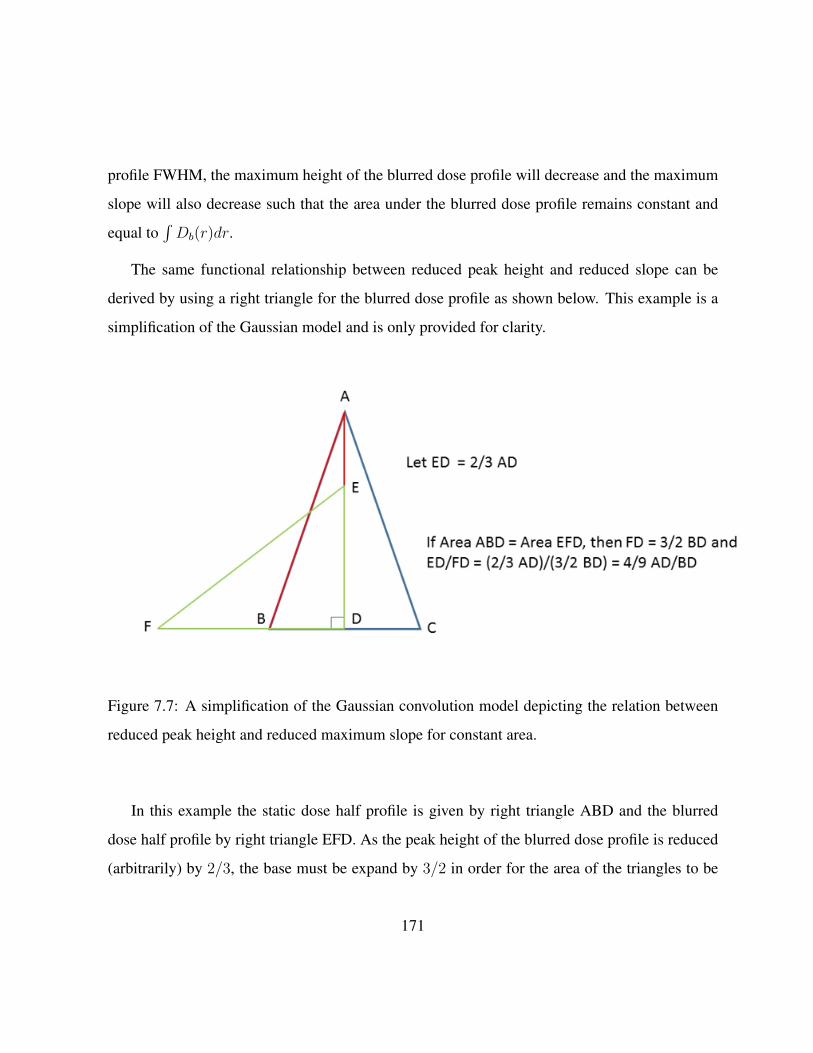
profile FWHM, the maximum height of the blurred dose profile will decrease and the maximum

slope will also decrease such that the area under the blurred dose profile remains constant and

equal to∫Db(r)dr.

The same functional relationship between reduced peak height and reduced slope can be

derived by using a right triangle for the blurred dose profile as shown below. This example is a

simplification of the Gaussian model and is only provided for clarity.

Figure 7.7: A simplification of the Gaussian convolution model depicting the relation between

reduced peak height and reduced maximum slope for constant area.

In this example the static dose half profile is given by right triangle ABD and the blurred

dose half profile by right triangle EFD. As the peak height of the blurred dose profile is reduced

(arbitrarily) by 2/3, the base must be expand by 3/2 in order for the area of the triangles to be

171

equal. For that situation, the slope of triangle EFD (relative to base FD) is given by ED/FD which

is equal to(23

)2 or 49

AD/BD which is the slope of the original static profile (relative to base BD).

The maximum blurred dose peak height curves in Figure 7.5 were generated from Equation

7.17. Each of the curves correspond to a different static dose FWHM ranging from 1.0 cm to

5.0 cm as shown in the legend. For each FWHM, the PDF standard deviation (σ1) was varied

from 0.1 cm to 1.0 cm. Power regression data fits were added to provide graphical verification

of the numeric analysis. As shown in Figure 7.5 the R values for each of the power regression

data fits are equal to 1 and the coefficients are the σ2 values that were calculated from integer

FWHM values using Equation 7.19.

The abscissa for both Figures 7.5 and 7.6 is labeled SD3 and corresponds to σ3 in the equa-

tions. For each of the curves in Figures 7.5 and 7.6, the range of applicable σ3 values decreases

as determined from Equation 7.14. The applicable σ3 range is defined as σ3|σ1=1.0 cmσ1=0.1 cm and is cal-

culated for each of the σ2 values corresponding to the integer static dose FWHM values. For

Figures 7.5 and 7.6, the applicable range of σ3 decreases from 0.65 cm at FWHM = 1.0 cm to

0.22 cm at FWHM = 5.0 cm.

Although the maximum height of the blurred dose profile for a given static FWHM decreases

as 1σ3

, the maximum peak height for constant σ1 increases as FWHM increases from 1.0 cm to

5.0 cm. From Equation 7.17, the maximum peak height is given by

(√1 +

(σ1σ2

)2)−1and the

limit as σ2 →∞ = 1.

This trend can be seen from Figure 7.5 and is described using the smallest and largest values

of σ1. For σ1 = 0.1 cm (lowest clinical PDF standard deviation studied), the maximum peak

height varies from 0.973 for FWHM = 1.0 cm to 0.999 for FWHM = 5.0 cm. For σ1 = 1.0 cm

(highest clinical PDF SD studied), the maximum peak height varies from 0.391 for FWHM =

1.0 cm to 0.905 for FWHM = 5.0 cm. The explanation for the relatively large drop in maximum

172

peak height for FWHM values of 1 cm and 2 cm is due to conservation of integral dose from

the convolution theorem explained previously (Equation 7.2). As the static dose profile FWHM

decreases to small values (e.g. 1 cm needed for SRS), and as the patients breathing becomes

more erratic (higher PDF standard deviation), the peak height drops below unity in addition to

an increase in the maximum slope in order to conserve the area under the blurred dose profile.

The drop in maximum peak dose height for static dose FWHM < 2.5 cm is discussed in more

detail in Section 5.

In Figure 7.6, the data for the maximum gradient of the blurred dose profile was generated

from Equation 7.6 using the same range of values for FWHM and σ1 as used to generate the

maximum peak height. Power regression data fits were also added to provide graphical verifica-

tion of the numeric analysis. Shown in Figure 7.6, the R values for each of the power regression

fits are equal to 1 and the coefficients are the σ2 values that were calculated from integer FWHM

values multiplied by e−0.5 = 0.607.

In contrast to the behavior of the maximum peak height, the maximum dose gradient for a

given static FWHM decreases as 1σ23, and the value of the maximum gradient for constant σ1

generally decreases with increasing FWHM. An exception to this trend occurs for σ1 ≥ 0.75 cm

as FWHM increases from 1.0 cm to 2.0 cm. For this situation as shown in Figure 7.6, there

is a small increase in the maximum blurred dose gradient which is again due to conservation of

integral dose. For the large drop in maximum peak height for FWHM = 1 cm and large σ1, there

is also a large decrease in the maximum dose gradient. As the FWHM increases from 1.0 cm

to 2.0 cm at large σ1 the maximum peak height increases and the maximum dose gradient must

increase slightly to conserve integral dose.

Derivatives of the blurred dose profiles are shown in Figures 7.8 and 7.9 for static dose

FWHM values of 2.6 cm and 5.1 cm. For both figures the derivatives are shown for σ1 values of

0.2, 0.5 and 0.8 cm.

173

Figure 7.8: The derivatives of the blurred Gaussian dose profiles generated from a static Gaussian

dose profile with FWHM of 2.6 cm and PDF standard deviations of 0.2 cm, 0.5 cm and 0.8 cm.

174

Figure 7.9: The derivatives of the blurred Gaussian dose profiles generated from a static Gaussian

dose profile with FWHM of 5.1 cm and PDF standard deviations of 0.2 cm, 0.5 cm and 0.8 cm.

For the Gaussian convolution model presented in this chapter the blurred dose profiles were

derived analytically to provide a parametric sensitivity analysis. This is in contrast to the method-

ology used in the thesis where the derivatives of the lung PDF were first convolved with the static

dose profile to obtain the blurred dose gradient and then integrated along the superior-inferior (r)

175

direction as described before. As shown in Figures 7.8 and 7.9, the derivatives of the blurred dose

distribution are symmetric, and, due to the peaked nature of the Gaussian static dose profile, the

transition of the derivatives from positive to negative is continuous through the origin with the

separation of the positive and negative peaks defining the blurred dose FWHM. For the Gaussian

convolution model there is no flat spot between the peaks of the blurred dose gradient as shown

in Figures 7.3 and 7.4 for a more flat static dose profile.

7.5 Table 6.2 Revisited

Table 6.2 in this thesis describes recommended margins to be applied to the static dose FWHM

in order to recover D95 that is lost due to lung motion quantified by the PDF standard deviation.

The table lists the ABW required as a function of FWHM and SD and is based on the quadratic

polynomial data fits shown in Table 6.1. The parametric boundaries of the Table 6.2 are 2.6 cm ≤

FWHM ≤ 10.1 cm and 0.1 cm ≤ SD ≤ 0.8 cm.

The recommended ABW data in Table 6.2 were plotted in Figure 7.10 as a function of the

FWHM of the static dose profile. Power regression data fits were added showing that the recom-

mended ABW varies approximately as 1√FWHM

(for fixed PDF standard deviation). This graph

was used to extend the experimental data to FWHM < 2.5 cm. The power regression equations

are tabulated in Table 7.1.

176

Figure 7.10: Plots of the recommended additional beam width from Table 6.2 as a function of

static profile FWHM for a range of fixed PDF standard deviations. The data presented here was

used to extend the experimental data to FWHM < 2.5 cm. In general, as the FWHM of the

static profile increases, the required additional beam width decreases for a given PDF standard

deviation.

The analytical convolution model presented in this chapter provides a reasonable benchmark

for testing the recommended margins in Table 6.2. For this investigation, the analytically simu-

177

PDF SD (cm) Fit equation of ABW data (mm) vs FWHM (cm) R2 of fit

0.1 ABW = 0.8903x−0.584 0.8511

0.2 ABW = 2.3039x−0.5 0.8339

0.3 ABW = 4.2274x−0.458 0.8438

0.4 ABW = 6.6367x−0.419 0.8810

0.5 ABW = 9.7082x−0.4 0.9157

0.6 ABW = 13.197x−0.381 0.9463

0.7 ABW = 17.563x−0.381 0.9547

0.8 ABW = 22.181x−0.369 0.9717

Table 7.1: A summary of equations describing the additional beam width (mm) versus FWHM

(cm) of the static Gaussian dose profiles for fixed PDF standard deviation.

lated blurred dose profile was computed using FWHM values for G2(r) and σ1 values for G1(r)

from Table 6.2 and compared with Equation 7.13 evaluated with the recommended margins ap-

plied to G2(r). The results are shown in Table 7.2 and graphically in Figures 7.11 and 7.12.

178

Figure 7.11: Analytically simulated static, blurred and ABW blurred dose profiles. The original

static profile had FHWM = 2.6 cm. The ABW recommended in this case is 1.6 cm. The loss of

dose coverage and the dose recovered by the ABW shown here is summarized in Table 7.2

179

Figure 7.12: Analytically simulated static, blurred and ABW blurred dose profiles. The original

static profile had FHWM = 5.1 cm. The ABW recommended in this case is 0.8 cm. The loss of

dose coverage and the dose recovered by the ABW shown here is summarized in Table 7.2

In the context of the analytical model presented,D95 has limited practicality and was replaced

with the dose deficit defined in Equation 7.5 and shown in Figure 7.2. To calculate the dose deficit

180

using Equation 7.5, the intersection points r∗ and r∗ were derived as follows.

By equating the motion-modified dose profile G4(r) = σ2√

2πG3(r) with the scaled static

dose profile G2(r) = 1σ2√2πe− 1

2

(rσ2

)2

• σ2√

2π the intersection points are given by

σ2σ3e− 1

2

(r∗σ3

)2

= e− 1

2

(r∗σ2

)2

. (7.20)

Solving for r∗ gives

r∗ = ±σ1σ2

√2(lnσ3 − lnσ2)

σ23 − σ2

2

. (7.21)

When Table 6.2 is applied to G2(r) such that FWHM = FWHM + ABW , the intersection

points of G2(r) and G3ABW (r) are given by

r∗ = ±σ1σ2

√2(lnσ3 − lnσ2ABW )

σ23 − σ2

2

, (7.22)

where G3ABW (r) and σ2ABW include ABW from Table 6.2.

For clarity in Table 7.2, r* is calculated from Equation 7.21 was labeled r1∗ and r∗ calculated

from Equation 7.22 was labeled r2∗. The initial deficit integral dose resulting from lung motion

was derived from

A1deficit =

∫ r1∗

−r1∗Do(r)−Db,ABW (r)dr, (7.23)

and residual deficit integral dose determined with recommended ABW from Table 6.2 was

derived from

181

A2deficit =

∫ r2∗

−r2∗Do(r)−Db,ABW (r)dr, (7.24)

where Db,ABW is the blurred dose with ABW.

Since the integral dose from Equation 7.23 includes the residual integral dose from Equation

7.24, the recovered dose from using the static dose profile with ABW was calculated using

RecoveredIntegralDose = 1−(A1deficitA2deficit

). (7.25)

The results and parametric details are shown in Table 7.2.

182

FWHM

(cm)

FWHM

+ ABW

σ1

(cm)

r1∗

(cm)

r2∗

(cm)

G2(r1∗)

(Gy)

G2(r2∗)

(Gy)

G3(0)

(Gy)G3,ABW (0)

(Gy)

A1deficit

(Gy cm)

A2deficit

(Gy cm)

Dose

Recov-

ery(1− A2

A1

)1.0 1.23 0.2 0.446 0.241 0.576 0.851 0.905 0.934 0.152 0.016 0.895

1.0 1.97 0.5 0.520 0.261 0.473 0.828 0.647 0.858 0.258 0.037 0.857

1.0 3.22 0.8 0.592 0.239 0.379 0.853 0.469 0.863 0.362 0.033 0.910

2.6 2.75 0.2 1.113 0.518 0.601 0.896 0.984 0.986 0.344 0.007 0.978

2.6 3.28 0.5 1.156 0.577 0.578 0.872 0.911 0.941 0.408 0.034 0.917

2.6 4.19 0.8 1.222 0.575 0.542 0.873 0.810 0.912 0.513 0.051 0.901

3.6 3.72 0.2 1.535 0.689 0.604 0.903 0.992 0.992 0.472 0.005 0.988

3.6 4.18 0.5 1.568 0.755 0.591 0.885 0.950 0.963 0.520 0.028 0.946

3.6 4.97 0.8 1.622 0.761 0.570 0.883 0.886 0.935 0.614 0.049 0.920

5.1 5.19 0.2 2.70 0.954 0.605 0.908 0.996 0.996 0.665 0.004 0.994

5.1 5.57 0.5 2.194 1.019 0.599 0.895 0.974 0.978 0.698 0.022 0.968

5.1 6.25 0.8 2.235 1.023 0.587 0.894 0.938 0.957 0.782 0.044 0.944

10.1 10.17 0.2 4.291 1.578 0.606 0.935 0.999 0.999 1.414 0.002 0.999

10.1 10.47 0.5 4.304 1.689 0.604 0.925 0.993 0.994 1.408 0.011 0.992

10.1 11.03 0.8 4.326 1.690 0.601 0.925 0.983 0.986 1.463 0.024 0.984

Table 7.2: A summary of the parametric analysis of the Gaussian convolution model. The legend is on the next

page.

183

• FWHM of the static dose profile

• FWHM + ABW added to static profile (per Table 6.2)

• SD1 is for static dose profile

• r1∗ is the intersection of blurred dose profile with static dose profile

• r2∗ is the intersection of blurred static profile including ABW with static dose profile

• G2(r1∗) is the value of static dose profile at r1∗

• G2(r2∗) is the value of static dose profile at r2∗

• G3(0) is max height of blurred dose profile at r = 0

• G3,ABW (0) is max height of blurred dose profile including ABW at r = 0

• A1deficit is integral dose lost due to target motion

• A2deficit is the integral dose lost to target motion after the field size has been increased per

Table 6.2

• Dose Recovery = 1− A2deficitA1deficit

When ABW from Table 6.2 motion is recovered within an average of 96% ± 2.5% for

0.1 cm ≤ σ1 ≤ 0.8 cm lung PDF and 2.6 cm ≤ FWHM ≤ 10.1 cm static dose profile. This

indicates that the ABW recommendations from Table 6.2, applied to the analytical Gaussian

convolution model, provide very good general recovery of the dose deficit resulting from organ

motion within the σ1 and FWHM parameters specified. For static dose profiles with FWHM

values less than 2.5 cm however (i.e. outside of the clinical parametric boundaries of Table 6.2),

dose recovery may not be practical using an ABW technique. As demonstrated previously, this

184

is due to a significant decrease in blurred dose maximum peak height and softer maximum dose

gradients arising from convolution of small static dose FWHM and large PDF SD. This extreme

is shown in Figures 7.13 to 7.15. In Figure 7.13, the ABW for FWHM = 1.0 cm was extrap-

olated from a power regression data fit shown in Figure 7.10. From Table 7.2, the recovered

integral dose for PDFSD = 0.8 cm is 0.91 which would be a problem clinically. Figures 7.14

and 7.15 show MATLAB simulations for small FWHM and large PDF standard deviations. In

Figure 7.15, the simulation is calculated for a rectangular dose pulse which is an ideal extreme

provided for comparison. A more clinical stereotactic static dose profile would be a cross be-

tween the Gaussian and rectangular profiles.

185

Figure 7.13: The effect of large target motion on a static Gaussian profile with FWHM of 1 cm.

This small target is particularly susceptible to loss of dose coverage as shown by the blurred dose

profile. The ABW recommendation derived from Figure 7.10 (or Table 7.1) is still insufficient to

restore full dose coverage for this small field and large motion

.

186

Figure 7.14: The effect of varying levels of target motion, represented by several PDF stan-

dard deviations, on a small field. As the amount of motion increases the dose coverage loss,

represented by the blurred dose profile, increases. The low dose spillage becomes an impor-

tant concern for small fields and large motion that may occur in the case of an SRS treatment

technique.

187

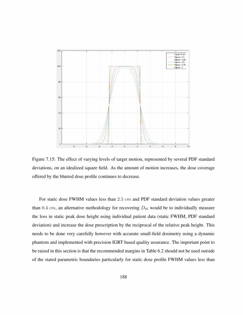
Figure 7.15: The effect of varying levels of target motion, represented by several PDF standard

deviations, on an idealized square field. As the amount of motion increases, the dose coverage

offered by the blurred dose profile continues to decrease.

For static dose FWHM values less than 2.5 cm and PDF standard deviation values greater

than 0.4 cm, an alternative methodology for recovering D95 would be to individually measure

the loss in static peak dose height using individual patient data (static FWHM, PDF standard

deviation) and increase the dose prescription by the reciprocal of the relative peak height. This

needs to be done very carefully however with accurate small-field dosimetry using a dynamic

phantom and implemented with precision IGRT based quality assurance. The important point to

be raised in this section is that the recommended margins in Table 6.2 should not be used outside

of the stated parametric boundaries particularly for static dose profile FWHM values less than

188

2.5 cm.

For static dose FWHM values greater than 2.5 cm and with flatter plateau regions as shown

in Figures 7.3 and 7.4, convolution with a PDF SD results mainly in a reduction of the dose

gradients at the leading and trailing edges, again conserving integral dose as described earlier.

This is shown in Figure 7.15 from a MATLAB simulation of a rectangular static dose profile with

FWHM = 5.0 cm. In this example the peak dose height does not start decreasing below 1.0 until

the PDFSD = 1.0 cm. Figure 7.16 shows the equivalent Gaussian static dose profile where the

maximum peak height starts decreasing for PDFSD = 0.5 cm due to the more peaked central

region. This comparison indicates that the Gaussian model, although very useful for developing

this sensitivity analysis, is more relevant clinically to SRS static dose profiles.

189

Figure 7.16: The effect of varying levels of target motion, represented by several PDF standard

deviations, on an idealized square field. As the amount of motion increases, the dose coverage

offered by the blurred dose profile continues to decrease. Due to the peaked nature of the Gaus-

sian profile, the maximum peak height begins to decrease with PDF standard deviation of 0.5 cm,

as compared to 1 cm for the equivalent square profile.

7.6 Summary

In this chapter a sensitivity analysis was presented of the convolution methodology used in this

thesis. Using a scaled Gaussian function for the static dose profile

190

G2(r) =1

σ2√

2πe− 1

2( rσ2

)2 • σ2√

2π, (7.26)

with a maximum peak height of 1.0, and a normalized Gaussian lung PDF with SD = σ1

G1(r) =1

σ1√

2πe− 1

2( rσ1

)2. (7.27)

The blurred dose profile was determined from the convolution of G1(r) and G2(r) and ana-

lyzed parametrically. The analytical solution of the blurred dose profile is also a Gaussian, and

was derived as

G4(r) = G2(r)⊗G1(r) =σ2σ3e− 1

2

(rσ3

)2

, (7.28)

with

σ3 =√σ21 + σ2

2. (7.29)

Summarizing the important results in this chapter;

1. the modified or blurred dose profile is given by the Gaussian function G4(r) with standard

deviation σ3 =√σ21 + σ2

2

2. the FWHM of the modified dose profile is given by FWHM = 2√

2ln2σ3

3. simultaneously

(a) the peak height of G4(r) varies as 1σ3

and

191

(b) the maximum slope of G4(r) varies as 1σ23

such that the integral dose is conserved via∫G4(r)dr =

∫G2(r)dr

4. generally, and governed by conservation of integral dose,

(a) the peak height of G4(r), or a given dose profile will decrease with increasing σ1

(b) the maximum slope of G4(r), for a given dose profile, will decrease with increasing

σ1

(c) the maximum peak height of G4(r), for a given σ1, will increase with increasing

FWHM of G2(r)

(d) the max slope ofG4(r), for a given σ1, will decrease with increasing FWHM ofG2(r)

5. additional beam width recommendations from Table 6.2 work reasonably well with the

analytical Gaussian blurred dose model. When the ABW is applied to the static dose

profile for a ”‘model-specific”’ PDF standard deviation and dose profile FWHM values,

the integral dose lost due to lung motion is recovered within an average of 96%± 2.5% for

0.1 cm ≤ σ1 ≤ 0.8 cm lung PDF standard deviation and 2.6 cm ≤ FHWM ≤ 10.1 cm

static dose profiles.

6. Table 6.2 should not be used clinically for static dose profiles and PDF standard deviations

outside of the parameter boundaries specified in item 5 above. For static dose FWHM <

2.5 cm, a patient-specific dosimetry workup should be performed to determine an estimate

for the loss of integral dose due to lung motion and an optimum strategy for providing

recovery.

192

Chapter 8

Conclusions

8.1 Discussion

Organ motion during the course of EBRT is a major source of geometric uncertainty in the

delivery of the prescribed radiation dose. Organ motion that occurs between fractions during

a radiotherapy treatment is known as interfraction motion. Organ motion that occurs during

treatment delivery is known as intrafraction motion. Both interfraction and intrafraction motion

need to be accounted for in order to accurately deliver the prescribed dose and achieve the best

patient outcomes. While interfraction motion can be effectively accounted for with daily imaging

on the treatment unit; compensating for intrafraction motion presents a larger challenge.

Addressing intrafraction motion continues to be a major concern for researchers and clin-

icians. Many approaches have been detailed in the literature, such as: breath-hold techniques,

gated radiotherapy, real time target tracking and motion encompassing techniques. While each of

these approaches has its advantages and disadvantages, motion encompassing techniques are the

most widely used due to the ease of implementation. Motion encompassing techniques seek to

193

define a treatment volume which sufficiently covers the volume represented by the target motion.

There have also been several approaches to motion encompassing techniques described in the

literature and each one seeks to balance the need to deliver sufficient dose to the target volume

while minimizing the dose to the surrounding OARs.

In this work, a motion encompassing technique to compensate for intrafraction lung motion

was developed. This technique is based on the convolution model of target motion. The convo-

lution model seeks to describe the effect of target motion on the delivered dose distribution by

convolving a planned static dose distribution and a probability distribution describing the target

motion. The convolution model was employed in the context of modern 4DCT equipment, which

offers new tools for assessing the impact of target motion. By generating the PDF from 4DCT

data and using the gradient of the PDF to obtain the blurred dose profiles, the effect of target

motion can be compensated for directly within the treatment planning environment.

The validity of the convolution model in the context of intrafraction motion was assessed with

radiochromic film measurements in a dynamic thorax phantom. This experimental validation

used regular and irregular breathing patterns recorded from patients as the source of the motion

pattern. After experimentally establishing the validity of the model, the model was employed as

part of a large simulation study to search for trends that can be used to guide treatment margin

selection to compensate for target motion in the lung.

The simulation study consisted of the analysis of the effect of 502 different patient breathing

patterns on targets ranging in diameter from 2.6 cm to 10.1 cm. An analysis of the dose coverage

resulting from the convolution model predictions lead to margin recommendations which seek to

maintain the minimum dose received by 95% of the target volume (D95). The margin recommen-

dations, as defined in Chapter 6, are based on the standard deviation of the target motion about

its mean position, and the diameter of the target volume.

194

A sensitivity analysis of the convolution model as applied to Gaussian dose profiles and

Gaussian breathing motion PDFs was presented. The sensitivity analysis of Gaussian functions

allows for an analytical approach to assess the effect of varying model parameters on the model

output. The analytical sensitivity analysis showed that the results derived in Chapter 6 have

limitations that need to be respected in extreme cases (small targets with large motion).

8.2 Summary of Key Results

The effect of target motion was investigated based on the breathing patterns recorded from 502

unique patients. The key results can be are summarized below:

• The two major assumptions of the convolution model are generally met when the model

is used in the context of intrafraction lung motion. The assumption of shift invariance was

considered in the context of intrafraction motion and meets the requirements as discussed

by other authors. The assumption of sufficient sampling in the context of intrafraction

motion was also assessed. Ultimately, sufficient sampling will be met for the vast majority

of cases given 10 s of beam on time. This was established with an empirical study of

patient breathing traces as well as a review of the convolution model limitations in the

literature.

• The accuracy of the convolution model predictions in the context of intrafraction lung

motion was established with radiochromic film measurements in a dynamic thorax phan-

tom. For both regular and irregular type breathing patterns, the convolution model makes

predictions accurate to within the 6% margin of error expected with good film handling

techniques.

195

• Breathing trace amplitudes used in this study ranged from 0.13 to 2.30 cm with an average

amplitude of 0.73 cm.

• Breathing trace PDF standard deviations used in this study ranged from 0.057 to 1.13 cm

with an average standard deviation of 0.34 cm.

• A reasonably strong correlation (R2 = 0.864) was found between breathing trace am-

plitude and standard deviation, indicating that the amplitude of the motion is the most

important factor in determining the breathing trace standard deviation.

• The loss of target dose coverage (D95) is well described by a quadratic function of the

breathing trace standard deviation. This relation indicates that loss of target D95 is negligi-

ble for breathing patterns with a standard deviation of less than 0.2 cm for all target sizes

(< 1% loss of target D95). In general, the loss of target D95 begins to become appreciable

for targets undergoing motion with a standard deviation of 0.4 cm or greater.

• The additional margin required to maintain target D95 can be computed by iteratively in-

creasing the beam width in the direction of motion, and computing the new relative D95 of

the blurred profile in each instance. A table of margin recommendations derived from this

simulation was presented in Chapter 6.

• Since the target D95 is a relative quantity dependent on the size of the target volume, the

role of target size in selecting these margins cannot be ignored. The results presented in the

margin recommendation table indicate that little to no extra margin is required for many

combinations of target size and level of motion.

• Target size plays an important role in loss of dose coverage. For targets with a FWHM

of 5 cm or greater, additional margin is only required for very large target motion (with

standard deviation ≥ 0.4 cm. For targets smaller than 5 cm, more care must be taken to

196

account for target motion. Small targets with large motion are by far the most susceptible

to loss of target dose coverage due to motion.

• The margin recommendations presented here can also be used to assess the trade off be-

tween target dose coverage and dose to OARs. If the margins recommended here would

cause unacceptable dose to an OAR, then the clinician can use that information do decided

whether the current treatment technique will be suitable.

• When the convolution model is applied to Gaussian PDFs and dose profiles, the results

presented in this thesis hold except for extreme cases of small targets with large motion.

8.3 Conclusion

Intrafraction target motion during external beam radiation therapy is a large source of geometric

uncertainty which has an impact on dose delivery. While technological advancements promise

new approaches to compensating for intrafraction motion, the most reliable and easiest to im-

plement of these approaches are the motion encompassing techniques. These techniques seek to

define an appropriate treatment margin to ensure the target volume receives the prescribed dose.

The expansion of treatment margins always comes at the cost of increased dose to OARs, and

so finding optimal margins is an important step in offering a successful radiotherapy treatment.

Offering patient specific recommendations for treatment margin selection allows for a fine bal-

ance to be struck between ensuring sufficient target dose and minimizing dose to the surrounding

OARs.

Intrafraction motion has the effect of ‘blurring’ the planned dose distribution causing a loss

of dose coverage to the target volume and increased dose to surrounding OARs upon treatment

delivery. The convolution model was found to accurately predict the loss of target dose coverage

197

due to the blurring of intrafraction motion. By assessing the loss of dose coverage in relation

to parameters of a given patient’s specific breathing, it was found that the standard deviation of

the breathing trace PDF is a useful predictor of the loss of dose coverage. For target motions

with a standard deviation ≥ 0.4 cm care should be taken to apply additional treatment margins

as described in Table 6.2.

The size of the target volume is an important factor when considering loss of dose coverage.

Small targets (< 5 cm) are most susceptible to a loss of dose coverage, while large targets

(> 5 cm) are more robust in the face of intrafraction motion. Finally, the gradient of the patient’s

breathing trace PDF offered insights into the blurring effect caused by the motion. The rate of

change of the PDF along the direction of motion highlights the features of the patient’s breathing

trace that will make the largest impact on the blurred dose distribution. While the PDF standard

deviation predicts the dominant blurring effect, the gradient of the PDF can offer insight into

asymmetries resulting from asymmetric breathing.

The results of this work further emphasize the need for patient specific approaches to margin

selection. The interplay between target size, dose gradients, PDF standard deviation, location

of the disease relative to OARs and treatment technique leaves no room for general solutions.

The margin recommendations made in this work can be used to help guide treatment planning

decisions by revealing the additional margin required to compensate for a given patient’s specific

breathing motion and target volume. By applying the margin at the treatment planning stage, the

impact on OARs for that patient’s disease site can be assessed. This type of patient specific ap-

proach can help ensure the patient receives the optimal treatment, and hence the best opportunity

for a successful treatment outcome.

198

8.4 Suggestions for Future Work

This line of research could be carried on through one of several veins of future work:

• The same approach to a motion encompassing technique could be applied to other cancer

sites susceptible to intrafraction target motion, such as the liver.

• The applicability of the model to segmented IMRT or volumetric modulated arc therapy

techniques could be assessed.

• Extending the work towards optimizing treatment margin selection based on radiobiologi-

cal considerations instead of purely physical (geometrical) considerations.

• Using the model predictions to adjust margins based on daily measured breathing patterns.

This could perhaps be extended to real time margin adjustments.

199

Bibliography

[1] M. Engelsmann, G. C. Sharp, T. Bortfeld, R. Onimaru, and H. Shirato. How much margin

reduction is possible through gating or breath hold? Physics in Medicine and Biology,

50(3):477–490, FEB 2005.

[2] Anne Richter, Kurt Baier, Juergen Meyer, Juergen Wilbert, Thomas Krieger, Michael

Flentje, and Matthias Guckenberger. Influence of increased target dose inhomogeneity

on margins for breathing motion compensation in conformal stereotactic body radiother-

apy. BMC Medical Physics, 8:5, DEC 2008.

[3] Eric J. Hall. Radiobiology for the radiologist. Philadelphia : Wolters Kluwer Health/Lip-

pincott Williams & Wilkins, Philadelphia, 7th edition, 2012.

[4] Harold E. Johns and John R. Cunningham. The Physics of Radiology. Charles C. Thomas,

1983, Springfield, Ill., U.S.A., 1983.

[5] Kazuhiro Yasufuku, Takahiro Nakajima, Ken Motoori, Yasuo Sekine, Kiyoshi Shibuya,

Kenzo Hiroshima, and Takehiko Fujisawa. Comparison of endobronchial ultrasound,

positron emission tomography, and CT for lymph node staging of lung cancer. Chest,

130(3):710–718, SEP 2006. PT: J; TC: 211; UT: WOS:000240585600018.

200

[6] T. Beyer, DW Townsend, T. Brun, PE Kinahan, M. Charron, R. Roddy, J. Jerin, J. Young,

L. Byars, and R. Nutt. A combined PET/CT scanner for clinical oncology. Journal of

Nuclear Medicine, 41(8):1369–1379, AUG 2000.

[7] G.C. Bentel. Radiation Therapy Planning. McGraw Hill, 2nd edition, 1996.

[8] JDP Hoisak, KE Sixel, R. Tirona, PCF Cheung, and JP Pignol. Correlation of lung tumor

motion with external surrogate indicators of respiration. International Journal of Radia-

tion Oncology Biology Physics, 60(4):1298–1306, NOV 2004.

[9] Y. Seppenwoolde, H. Shirato, K. Kitamura, S. Shimizu, M. van Herk, JV Lebesque, and

K. Miyasaka. Precise and real-time measurement of 3D tumor motion in lung due to

breathing and heartbeat, measured during radiotherapy. International Journal of Radiation

Oncology Biology Physics, 53(4):822–834, JUL 2002.

[10] Katharina E. Sixel, Mark Ruschin, Romeo Tirona, and Patrick C. F. Cheung. Digital

fluoroscopy to quantify lung tumor motion: Potential for patient-specific planning target

volumes. International Journal of Radiation Oncology Biology Physics, 57(3):717–723,

2003.

[11] H. Shirato, K. Suzuki, G. C. Sharp, K. Fujita, R. Onimaru, M. Fujino, N. Kato, Y. Osaka,

R. Kinoshita, H. Taguchi, S. Onodera, and K. Miyasaka. Speed and amplitude of lung

tumor motion precisely detected in four-dimensional setup and in real-time tumor-tracking

radiotherapy. International Journal of Radiation Oncology Biology Physics, 64(4):1229–

1236, 2006.

[12] Paul J. Keall, Gig S. Mageras, James M. Balter, Richard S. Emery, Kenneth M. Forster,

Steve B. Jiang, Jeffrey M. Kapatoes, Daniel A. Low, Martin J. Murphy, Brad R. Murray,

Chester R. Ramsey, Marcel B. Van Herk, S. S. Vedam, John W. Wong, and Ellen Yorke.

201

The management of respiratory motion in radiation oncology report of AAPM Task Group

76. Medical Physics, 33(10):3874–3900, OCT 2006.

[13] Marcel van Herk, Peter Remeijer, Coen Rasch, and Joos V. Lebesque. The probability

of correct target dosage: Dose-population histograms for deriving treatment margins in

radiotherapy. International Journal of Radiation Oncology Biology Physics, 47(4):1121–

1135, 2000.

[14] JY Jin, M. Ajlouni, Q. Chen, FF Yin, and B. Movsas. A technique of using gated-CT

images to determine internal target volume (ITV) for fractionated stereotactic lung radio-

therapy. Radiotherapy and Oncology, 78(2):177–184, FEB 2006.

[15] H. H. Liu, Peter Balter, Teresa Tutt, Bum Choi, Joy Zhang, Catherine Wang, Melinda

Chi, Dershan Luo, Tinsu Pan, Sandeep Hunjan, George Starkschall, Isaac Rosen, Karl

Prado, Zhongxing Liao, Joe Chang, Ritsuko Komaki, James D. Cox, Radhe Mohan, and

Lei Dong. Assessing respiration-induced tumor motion and internal target volume using

four-dimensional computed tomography for radiotherapy of lung cancer. International

Journal of Radiation Oncology Biology Physics, 68(2):531–540, JUN 2007.

[16] Emily Heath, Jan Unkelbach, and Uwe Oelfke. Incorporating uncertainties in respiratory

motion into 4D treatment plan optimization. Medical Physics, 36(7):3059–3071, JUL

2009.

[17] H. D. Kubo and B. C. Hill. Respiration gated radiotherapy treatment: A technical study.

Physics in Medicine and Biology, 41(1):83–91, JAN 1996.

[18] L. Ekberg, O. Holmberg, L. Wittgren, G. Bjelkengren, and T. Landberg. What margins

should be added to the clinical target volume in radiotherapy treatment planning for lung

cancer? Radiotherapy and Oncology, 48(1):71–77, JUL 1998.

202

[19] M. Engelsmann, E. M. F. Damen, K. De Jaeger, K. M. van Ingen, and B. J. Mijnheer. The

effect of breathing and set-up errors on the cumulative dose to a lung tumor. Radiotherapy

and Oncology, 60(1):95–105, JUL 2001.

[20] S. S. Vedam, V. R. Kini, P. J. Keall, V. Ramakrishnan, H. Mostafavi, and R. Mohan.

Quantifying the predictability of diaphragm motion during respiration with a noninvasive

external marker. Medical Physics, 30(4):505–513, APR 2003.

[21] E. Rietzel, G. T. Y. Chen, N. C. Choi, and C. G. Willet. Four-dimensional image-based

treatment planning: Target volume segmentation and dose calculation in the presence

of respiratory motion. International Journal of Radiation Oncology Biology Physics,

61(5):1535–1550, APR 2005.

[22] J. Leong. Implementation of random positioning error in computerized radiation treatment

planning systems as a result of fractionation. Physics in Medicine and Biology, 32(3):327–

334, MAR 1987.

[23] A. E. Lujan, E. W. Larsen, J. M. Balter, and R. K. Ten Haken. A method for incorporating

organ motion due to breathing into 3D dose calculations. Medical Physics, 26(5):715–720,

MAY 1999.

[24] Runqing Jiang, Rob B. Barnett, James C. L. Chow, and Jeff Z. Y. Chen. The use of

spatial dose gradients and probability density function to evaluate the effect of internal

organ motion for prostate IMRT treatment planning. Physics in Medicine and Biology,

52(5):1469–1484, MAR 2007.

[25] Jiang Hsieh. Computed tomography principles, design, artifacts, and recent advances /.

Bellingham, Wash. (1000 20th St. Bellingham WA 98225-6705 USA) : SPIE, c2009, 2nd

edition, 2009.

203

[26] Jerrold T. Bushberg. The essential physics of medical imaging. Philadelphia : Lippincott

Williams & Wilkins, Philadelphia, 2nd edition, 2002.

[27] Nicholas Denko, Amato Giaccia, Bruce Peters, and Thomas D. Stamato. An asymmetric

field inversion gel electrophoresis method for the separation of large DNA molecules.

Analytical Biochemistry, 178(1):172–176, APR 1989.

[28] Thomas D. Stamato and Nicholas Denko. Asymmetric field inversion gel electrophoresis:

A new method for detecting DNA double-strand breaks in mammalian cells. Radiation

research, 121(2):196–205, FEB 1990.

[29] E. B. Podgorak. Radiation physics for medical physicists. Heidelberg : Springer, c2010,

2nd edition, 2010.

[30] B. G. Douglas and J. F. Fowler. The effect of multiple small doses of x-rays on skin

reactions in the mouse and a basic interpretation. Radiation Research, 66(2):401–426,

May 1976.

[31] J. C. Mottram. A factor of importance in the radio sensitivity of tumours. The British

Journal of Radiology, 9(105):606–614, 1936.

[32] John Read. The effect of ionizing radiations on the broad bean root, part X. The British

Journal of Radiology, 25(290):89–99, 1952.

[33] J. B. Little, G. M. Hahn, E. Frindel, and M. Tubiana. Repair of potentially lethal radiation-

damage in-vitro and in-vivo. Radiology, 106(3):689–694, 1973.

[34] M. M. Elkind, Suttongi.H, W. B. Moses, T. Alescio, and R. W. Swain. Radiation response

of mammalian cells crown in culture .V. Temperature dependence of repair of x-ray dam-

age in surviving cells ( aerobic and hypoxic ). Radiation research, 25(2):359–376, 1965.

204

[35] J. F. Fowler. Fractionated radiation therapy after strandqvist. Acta Radiologica Oncology,

23(4):209–216, 1984.

[36] T. R. Munro and C. W. Gilbert. The relation between tumour lethal doses and the ra-

diosensitivity of tumour cells. British Journal of Radiology, 34(400):246–251, 1961.

[37] S. Webb and A. E. Nahum. A model for calculating tumor-control probability in ra-

diotherapy including the effects of inhomogeneous distributions of dose and clonogenic

cell-density. Physics in Medicine and Biology, 38(6):653–666, JUN 1993.

[38] J. T. Lyman. Complication probability as assessed from dose volume histograms. Radia-

tion research, 104(2):S13–S19, 1985 1985.

[39] C. Burman, G. J. Kutcher, B. Emami, and M. Goitein. Fitting of normal tissue tolerance

data to an analytic function. International journal of radiation oncology, biology, physics,

21(1):123–135, MAY 1991.

[40] Canadian Cancer Society; 2013 Canadian Cancer Society’s Advisory Committee on Can-

cer Statistics. Toronto. Canadian cancer statistics 2013.

[41] Taimur Sher, Grace K. Dy, and Alex A. Adjei. Small cell lung cancer. Mayo Clinic

Proceedings, 83(3):355–367, MAR 2008.

[42] G. Otterson, A. Lin, and F. Kay. Genetic etiology of lung cancer. Oncology (Williston

Park, N.Y.), 6(9):97–104, 107; Discussion 108, 111–2, SEP 1992.

[43] Julian R. Molina, Piii G. Yang, Stephen D. Cassivi, Steven E. Schild, and Alex A. Adjei.

Non-small cell lung cancer: Epidemiology, risk factors, treatment, and survivorship. Mayo

Clinic Proceedings, 83(5):584–594, MAY 2008.

205

[44] Robert Timmerman, Rebecca Paulus, James Galvin, Jeffrey Michalski, William Straube,

Jeffrey Bradley, Achilles Fakiris, Andrea Bezjak, Gregory Videtic, David Johnstone, Jack

Fowler, Elizabeth Gore, and Hak Choy. Stereotactic body radiation therapy for inoperable

early stage lung cancer. Journal of the American Medical Association, 303(11):1070–

1076, MAR 2010.

[45] CF Mountain. Revisions in the international system for staging lung cancer. Chest,

111(6):1710–1717, 1997.

[46] W. T. Sause, C. Scott, S. Taylor, D. Johnson, R. Livingston, R. Komaki, B. Emami, W. J.

Curran, R. W. Byhardt, A. T. Turrisi, A. R. Dar, and J. D. Cox. Radiation-Therapy-

Oncology-Group (RTOG)-88-08 and Eastern-Cooperative-Oncology-Group (ECOG)-

4588 - preliminary-results of a phase-III trial in regionally advanced, unresectable non-

small-cell lung-cancer. Journal of the National Cancer Institute, 87(3):198–205, FEB

1995.

[47] B. Emami, J. Lyman, A. Brown, L. Coia, M. Goitein, J. E. Munzenrider, B. Shank, L. J.

Solin, and M. Wesson. Tolerance of normal tissue to therapeutic irradiation. International

Journal of Radiation Oncology Biology Physics, 21(1):109–122, MAY 1991.

[48] Lawrence B. Marks, Soren M. Bentzen, Joseph O. Deasy, Feng-Ming Kong, Jeffrey D.

Bradley, Ivan S. Vogelius, Issam El Naqa, Jessica L. Hubbs, Joos V. Lebesque, Robert D.

Timmerman, Mary K. Martel, and Andrew Jackson. Radiation dose-volume effects in

the lung. International Journal of Radiation Oncology Biology Physics, 76(3):S70–S76,

2010.

206

[49] Giovanna Gagliardi, Louis S. Constine, Vitali Moiseenko, Candace Correa, Lori J. Pierce,

Aaron M. Allen, and Lawrence B. Marks. Radiation dose-volume effects in the heart.

International Journal of Radiation Oncology Biology Physics, 76(3):S77–S85, 2010.

[50] John P. Kirkpatrick, Albert J. van der Kogel, and Timothy E. Schultheiss. Radiation dose-

volume effects in the spinal cord. International Journal of Radiation Oncology Biology

Physics, 76(3):S42–S49, 2010.

[51] Maria Werner-Wasik, Ellen Yorke, Joseph Deasy, Jiho Nam, and Lawrence B. Marks.

Radiation dose-volume effects in the esophagus. International Journal of Radiation On-

cology Biology Physics, 76(3):S86–S93, 2010.

[52] Paiman Ghafoori, Lawrence B. Marks, Zeljko Vujaskovic, and Christopher R. Kelsey.

Radiation-induced lung injury - assessment, management, and prevention. Oncology-New

York, 22(1):37–47, JAN 2008.

[53] Karen Breitman, Satyapal Rathee, Chris Newcomb, Brad Murray, Don Robinson, Colin

Field, Heather Warkentin, Sherry Connors, Marc MacKenzie, Peter Dunscombe, and Gino

Fallone. Experimental validation of the Eclipse AAA algorithm. Journal of Applied

Clinical Medical Physics, 8(2):76–92, 2007.

[54] N. Childress, E. Stevens, D. Eklund, and M. Zhang. Mobius3D white paper: Dose calcu-

lation algorithm.

[55] James C. L. Chow, Michael K. K. Leung, and Jake Van Dyk. Variations of lung density and

geometry on inhomogeneity correction algorithms: A Monte Carlo dosimetric evaluation.

Medical Physics, 36(8):3619–3630, AUG 2009.

[56] Brandon Disher, George Hajdok, Stewart Gaede, and Jerry J. Battista. An in-depth Monte

Carlo study of lateral electron disequilibrium for small fields in ultra-low density lung:

207

implications for modern radiation therapy. Physics in Medicine and Biology, 57(6):1543–

1559, MAR 2012.

[57] Petra S. Kroon, Sandra Hol, and Marion Essers. Dosimetric accuracy and clinical quality

of Acuros XB and AAA dose calculation algorithm for stereotactic and conventional lung

volumetric modulated arc therapy plans. Radiation Oncology, 8:149, JUN 2013.

[58] S. Webb. Motion effects in (intensity modulated) radiation therapy: a review. Physics in

Medicine and Biology, 51(13):R403–R425, JUL 2006.

[59] G. S. Mageras, E. Yorke, K. Rosenzweig, L. Braban, E. Keatley, E. Ford, S. A. Leibel, and

C. C. Ling. Fluoroscopic evaluation of diaphragmatic motion reduction with a respiratory

gated radiotherapy system. Journal of Applied Clinical Medical Physics, 2(4):191–200,

2001.

[60] Jean-Pierre Bissonnette, Kevin N. Franks, Thomas G. Purdie, Douglas J. Moseley, Jan-

Jakob Sonke, David A. Jaffray, Laura A. Dawson, and Andrea Bezjak. Quantifying

interfraction and intrafraction tumor motion in lung stereotactic body radiotherapy us-

ing respiration-correlated cone beam computed tomography. International Journal of

Radiation Oncology Biology Physics, 75(3):688–695, NOV 2009. PT: J; TC: 44; UT:

WOS:000270573100008.

[61] G. S. Mageras, A. Pevsner, E. D. Yorke, K. E. Rosenzweig, E. C. Ford, A. Hertanto,

S. M. Larson, D. M. Lovelock, Y. E. Erdi, S. A. Nehmeh, J. L. Humm, and C. C. Ling.

Measurement of lung tumor motion using respiration-correlated CT. International Journal

of Radiation Oncology Biology Physics, 60(3):933–941, 2004.

[62] C. Plathow, S. Ley, C. Fink, M. Puderbach, W. Hosch, A. Schmahl, J. Debus, and H. U.

Kauczor. Analysis of intrathoracic tumor mobility during whole breathing cycle by dy-

208

namic MRI. International Journal of Radiation Oncology Biology Physics, 59(4):952–

959, JUL 2004.

[63] M. J. Murphy, D. Martin, R. Whyte, J. Hai, C. Ozhasoglu, and Q. T. Le. The effectiveness

of breath-holding to stabilize lung and pancreas tumors during radiosurgery. International

Journal of Radiation Oncology Biology Physics, 53(2):475–482, JUN 2002.

[64] Yelin Suh, Sonja Dieterich, Byungchul Cho, and Paul J. Keall. An analysis of thoracic and

abdominal tumour motion for stereotactic body radiotherapy patients. Physics in Medicine

and Biology, 53(13):3623–3640, JUL 2008.

[65] Keiichi Nakagawa, Akihiro Haga, Satoshi Kida, Yoshitaka Masutani, Hideomi Yamashita,

Wataru Takahashi, Akira Sakumi, Naoya Saotome, Takashi Shiraki, Kuni Ohtomo, Yoshio

Iwai, and Kiyoshi Yoda. 4D registration and 4D verification of lung tumor position for

stereotactic volumetric modulated arc therapy using respiratory-correlated cone-beam CT.

Journal of Radiation Research, 54(1):152–156, JAN 2013.

[66] Lars Dietrich, Siri Jetter, Thomas Tuecking, Simeon Nill, and Uwe Oelfke. Linac-

integrated 4D cone beam CT: first experimental results. Physics in Medicine and Biology,

51(11):2939–2952, JUN 2006.

[67] T. Pan, TY Lee, E. Rietzel, and GTY Chen. 4D-CT imaging of a volume influenced by

respiratory motion on multi-slice CT. Medical Physics, 31(2):333–340, FEB 2004.

[68] Vijay R. Kini, Subrahmanya S. Vedam, Paul J. Keall, Sumukh Patil, Clayton Chen, and

Radhe Mohan. Patient training in respiratory-gated radiotherapy. Medical Dosimetry:

Official Journal of the American Association of Medical Dosimetrists, 28(1):7–11, 2003.

209

[69] Stine S. Korreman, Trine Juhler-Nottrup, and Arthur L. Boyer. Respiratory gated beam

delivery cannot facilitate margin reduction, unless combined with respiratory correlated

image guidance. Radiotherapy and Oncology, 86(1):61–68, JAN 2008.

[70] CA; 2007 Varian Medical Systems Inc., Palo Alto. RPM respiratory gating system refer-

ence guide.

[71] Kristin J. Redmond, Danny Y. Song, Jana L. Fox, Jessica Zhou, C. N. Rosenzweig, and

Eric Ford. Respiratory motion changes of lung tumors over the course of radiation therapy

based on respiration-correlated four-dimensional computed tomography scans. Interna-

tional Journal of Radiation Oncology, Biology, Physics, 75(5):1605–1612, DEC 2009.

[72] Thomas G. Purdie, Jean-Pierre Bissonnette, Kevin Franks, Andrea Bezjak, David Payne,

Fanny Sie, Michael B. Sharpe, and David A. Jaffray. Cone-beam computed tomog-

raphy for on-line image guidance of lung stereotactic radiotherapy: Localization, ver-

ification, and intrafraction tumor position. International Journal of Radiation On-

cology Biology Physics, 68(1):243–252, MAY 1 2007 2007. PT: J; TC: 125; UT:

WOS:000246046000033.

[73] F. J. Lagerwaard, J. R. V. de Koste, M. R. J. Nijssen-Visser, R. H. Schuchhard-Schipper,

S. S. Oei, A. Munne, and S. Senan. Multiple ‘slow’ CT scans for incorporating lung tumor

mobility in radiotherapy planning. International Journal of Radiation Oncology Biology

Physics, 51(4):932–937, NOV 2001.

[74] J. Hanley, M. M. Debois, D. Mah, G. S. Mageras, A. Raben, K. Rosenzweig, B. Mychal-

czak, L. H. Schwartz, P. J. Gloeggler, W. Lutz, C. C. Ling, S. A. Leibel, Z. Fuks, and G. J.

Kutcher. Deep inspiration breath-hold technique for lung tumors: The potential value of

210

target immobilization and reduced lung density in dose escalation. International Journal

of Radiation Oncology Biology Physics, 45(3):603–611, OCT 1999.

[75] R. W. M. Underberg, F. J. Lagerwaard, B. J. Slotman, J. P. Cuijpers, and S. Senan. Use

of maximum intensity projections (MIP) for target volume generation in 4DCT scans for

lung cancer. International Journal of Radiation Oncology Biology Physics, 63(1):253–

260, SEP 2005.

[76] N. L. Ford, M. M. Thornton, and D. W. Holdsworth. Fundamental image quality limits for

microcomputed tomography in small animals. Medical physics, 30(11):2869–2877, NOV

2003.

[77] E. C. Ford, G. S. Mageras, E. Yorke, and C. C. Ling. Respiration-correlated spiral CT: A

method of measuring respiratory-induced anatomic motion for radiation treatment plan-

ning. Medical Physics, 30(1):88–97, JAN 2003.

[78] E. Rietzel, TS Pan, and GTY Chen. Four-dimensional computed tomography: Image

formation and clinical protocol. Medical Physics, 32(4):874–889, APR 2005.

[79] X. A. Li, C. Stepaniak, and E. Gore. Technical and dosimetric aspects of respiratory gating

using a pressure-sensor motion monitoring system. Medical Physics, 33(1):145–154, JAN

2006.

[80] Matthias Guckenberger, Juergen Wilbert, Thomas Krieger, Anne Richter, Kurt Baier, and

Michael Flentje. Mid-ventilation concept for mobile pulmonary tumors: Internal tu-

mor trajectory versus selective reconstruction of four-dimensional computed tomography

frames based on external breathing motion. International Journal of Radiation Oncology

Biology Physics, 74(2):602–609, JUN 2009.

211

[81] Joseph P. Santoro, Ellen Yorke, Karyn A. Goodman, and Gig S. Mageras. From phase-

based to displacement-based gating: A software tool to facilitate respiration-gated radia-

tion treatment. Journal of Applied Clinical Medical Physics, 10(4):132–141, 2009.

[82] A. F. Abdelnour, S. A. Nehmeh, T. Pan, J. L. Humm, P. Vernon, H. Schoder, K. E. Rosen-

zweig, G. S. Mageras, E. Yorke, S. M. Larson, and Y. E. Erdi. Phase and amplitude

binning for 4D-CT imaging. Physics in Medicine and Biology, 52(12):3515–3529, JUN

2007.

[83] E. Rietzel and G. T. Y. Chen. Improving retrospective sorting of 4D computed tomography

data. Medical Physics, 33(2):377–379, FEB 2006.

[84] Hua Li, Camille Noel, Jose Garcia-Ramirez, Daniel Low, Jeffrey Bradley, Clifford Robin-

son, Sasa Mutic, and Parag Parikh. Clinical evaluations of an amplitude-based binning

algorithm for 4DCT reconstruction in radiation therapy. Medical physics, 39(2):922–932,

FEB 2012.

[85] Jeffrey R. Olsen, Wei Lu, James P. Hubenschmidt, Michelle M. Nystrom, Paul Klahr, Jef-

frey D. Bradley, Daniel A. Low, and Parag J. Parikh. Effect of novel amplitude/phase

binning algorithm on commercial four-dimensional computed tomography quality. Inter-

national Journal of Radiation Oncology Biology Physics, 70(1):243–252, JAN 2008.

[86] Wei Lu, Parag J. Parikh, James P. Hubenschmidt, Jeffrey D. Bradley, and Daniel A. Low. A

comparison between amplitude sorting and phase-angle sorting using external respiratory

measurement for 4D CT. Medical Physics, 33(8):2964–2974, AUG 2006.

[87] Nicole M. Wink, Christoph Panknin, and Timothy D. Solberg. Phase versus amplitude

sorting of 4D-CT data. Journal of Applied Clinical Medical Physics, 7(1):77–85, 2006.

212

[88] ICRU Report 50. International commission on radiation units and measurements.

Bethesda, MD, 1993.

[89] ICRU Report 62. International commission on radiation units and measurements.

Bethesda, MD, 1999.

[90] D. Mah, J. Hanley, K. E. Rosenzweig, E. Yorke, L. Braban, C. C. Ling, S. A. Leibel, and

G. Mageras. Technical aspects of the deep inspiration breath-hold technique in the treat-

ment of thoracic cancer. International Journal of Radiation Oncology Biology Physics,

48(4):1175–1185, NOV 2000.

[91] J. W. Wong, M. B. Sharpe, D. A. Jaffray, J. M. Robertson, J. S. Stromberg, V. R. Kini, and

A. A. Martinez. The use of active breathing control (ABC) to minimize breathing motion

during radiation therapy. International Journal of Radiation Oncology Biology Physics,

39(2):164–164, 1997.

[92] Y. Negoro, Y. Nagata, T. Aoki, T. Mizowaki, N. Araki, K. Takayama, M. Kokubo, S. Yano,

S. Koga, K. Sasai, Y. Shibamoto, and M. Hiraoka. The effectiveness of an immobiliza-

tion device in conformal radiotherapy for lung tumor: Reduction of respiratory tumor

movement and evaluation of the daily setup accuracy. International Journal of Radiation

Oncology Biology Physics, 50(4):889–898, JUL 2001.

[93] H. D. Kubo, P. M. Len, S. Minohara, and H. Mostafavi. Breathing-synchronized radio-

therapy program at the University of California Davis Cancer Center. Medical Physics,

27(2):346–353, FEB 2000.

[94] S. Shimizu, H. Shirato, S. Ogura, H. Akita-Dosaka, K. Kitamura, T. Nishioka, K. Kagei,

M. Nishimura, and K. Miyasaka. Detection of lung tumor movement in real-time tumor-

213

tracking radiotherapy. International Journal of Radiation Oncology Biology Physics,

51(2):304–310, OCT 2001.

[95] Q. S. Chen, M. S. Weinhous, F. C. Deibel, J. P. Ciezki, and R. M. Macklis. Fluoroscopic

study of tumor motion due to breathing: Facilitating precise radiation therapy for lung

cancer patients. Medical Physics, 28(9):1850–1856, SEP 2001.

[96] S. Ahn, B. Yi, Y. Suh, J. Kim, S. Lee, S. Shin, S. Shin, and E. Choi. A feasibility study

on the prediction of tumour location in the lung from skin motion. British Journal of

Radiology, 77(919):588–596, JUL 2004.

[97] A. Schweikard, G. Glosser, M. Bodduluri, M. J. Murphy, and J. R. Adler. Robotic motion

compensation for respiratory movement during radiosurgery. Computer Aided Surgery,

5(4):263–77, 2000.

[98] T. Neicu, H. Shirato, Y. Seppenwoolde, and S. B. Jiang. Synchronized moving aper-

ture radiation therapy (SMART): Average tumour trajectory for lung patients. Physics in

Medicine and Biology, 48(5):587–598, MAR 2003.

[99] P. J. Keall, V. R. Kini, S. S. Vedam, and R. Mohan. Motion adaptive x-ray therapy: A

feasibility study. Physics in Medicine and Biology, 46(1):1–10, JAN 2001.

[100] W. D. D’Souza, S. A. Naqvi, and C. X. Yu. Real-time intra-fraction-motion tracking using

the treatment couch: a feasibility study. Physics in Medicine and Biology, 50(17):4021–

4033, SEP 2005.

[101] PJ Keall, S. Joshi, SS Vedam, JV Siebers, VR Kini, and R. Mohan. Four-dimensional

radiotherapy planning for DMLC-based respiratory motion tracking. Medical Physics,

32(4):942–951, APR 2005.

214

[102] R. W. M. Underberg, F. J. Lagerwaard, J. P. Cuijpers, B. J. Slotman, J. R. V. de Koste, and

S. Senan. Four-dimensional CT scans for treatment planning in stereotactic radiotherapy

for stage I lung cancer. International Journal of Radiation Oncology Biology Physics,

60(4):1283–1290, NOV 2004.

[103] Marjan A. Admiraal, Danny Schuring, and Coen W. Hurkmans. Dose calculations ac-

counting for breathing motion in stereotactic lung radiotherapy based on 4D-CT and the

internal target volume. Radiotherapy and Oncology, 86(1):55–60, JAN 2008.

[104] Stuart S. C. Burnett, Katharina E. Sixel, Patrick C. F. Cheung, and Jeremy D. P. Hoisak.

A study of tumor motion management in the conformal radiotherapy of lung cancer. Ra-

diotherapy and Oncology, 86(1):77–85, JAN 2008.

[105] Johan P. Cuijpers, Wilko F. A. R. Verbakel, Ben J. Slotman, and Suresh Senan. A novel

simple approach for incorporation of respiratory motion in stereotactic treatments of lung

tumors. Radiotherapy and Oncology, 97(3):443–448, DEC 2010.

[106] J. Unkelbach and U. Oelfke. Inclusion of organ movements in IMRT treatment planning

via inverse planning based on probability distributions. Physics in Medicine and Biology,

49(17):4005–4029, SEP 2004.

[107] Ronald N. (. N. Bracewell. The Fourier transform and its applications. Boston : McGraw

Hill, Boston, 3rd edition, 2000. ID: vtug3194985; Includes bibliographical references and

index.

[108] 1922 Arfken, George B. (. B. Mathematical methods for physicists. Elsevier; Elsevier

Academic Press, Boston; Amsterdam ; Burlington, MA, 6th ed. / george b. arfken, hans j.

weber. edition, 2005. ID: dedupmrg405584022; Includes bibliographical references and

index.

215

[109] T. Craig, J. Battista, and J. Van Dyk. Limitations of a convolution method for modeling

geometric uncertainties in radiation therapy. I. The effect of shift invariance. Medical

Physics, 30(8):2001–2011, AUG 2003.

[110] T. Craig, J. Battista, and J. Van Dyk. Limitations of a convolution method for modeling

geometric uncertainties in radiation therapy. II. The effect of a finite number of fractions.

Medical Physics, 30(8):2012–2020, AUG 2003.

[111] Jochem W. H. Wolthaus, Christoph Schneider, Jan-Jakob Sonke, Marcel van Herk, Jose

S. A. Belderbos, Maddalena M. G. Rossi, Joos V. Lebesque, and Eugene M. F. Damen.

Mid-ventilation CT scan construction from four-dimensional respiration-correlated CT

scans for radiotherapy planning of lung cancer patients. International Journal of Radiation

Oncology Biology Physics, 65(5):1560–1571, AUG 2006.

[112] T. Bortfeld, K. Jokivarsi, M. Goitein, J. Kung, and S. B. Jiang. Effects of intra-fraction

motion on IMRT dose delivery: statistical analysis and simulation. Physics in Medicine

and Biology, 47(13):2203–2220, JUL 2002.

[113] C. X. Yu, D. A. Jaffray, and J. W. Wong. The effects of intra-fraction organ motion on the

delivery of dynamic intensity modulation. Physics in Medicine and Biology, 43(1):91–

104, JAN 1998.

[114] C. S. Chui, E. Yorke, and L. Hong. The effects of intra-fraction organ motion on the deliv-

ery of intensity-modulated field with a multileaf collimator. Medical Physics, 30(7):1736–

1746, JUL 2003.

[115] Haisen S. Li, Indrin J. Chetty, and Timothy D. Solberg. Quantifying the interplay effect in

prostate IMRT delivery using a convolution-based method. Medical Physics, 35(5):1703–

1710, MAY 2008.

216

[116] M. Rosu, L. A. Dawson, J. M. Balter, D. L. McShan, T. S. Lawrence, and R. K. T. Haken.

Alterations in normal liver doses due to organ motion. International Journal of Radiation

Oncology Biology Physics, 57(5):1472–1479, DEC 2003.

[117] J. M. Balter, K. K. Brock, K. L. Lam, D. Tatro, L. A. Dawson, D. McShan, and R. K.

Ten Haken. Evaluating the influence of setup uncertainties on treatment planning for focal

liver tumors. International Journal of Radiation Oncology Biology Physics, 63(2):610–

614, OCT 2005.

[118] E. Astreinidou, A. Bel, CPJ Raaijmakers, CHJ Terhaard, and JJW Lagendijk. Adequate

margins for random setup uncertainties in head-and-neck IMRT. International Journal of

Radiation Oncology Biology Physics, 61(3):938–944, MAR 2005.

[119] J. V. Siebers, P. J. Keall, Q. W. Wu, J. F. Williamson, and R. K. Schmidt-Ullrich. Effect

of patient setup errors on simultaneously integrated boost head and neck IMRT treatment

plans. International Journal of Radiation Oncology Biology Physics, 63(2):422–433, OCT

2005.

[120] J. M. Balter, R. K. TenHaken, T. S. Lawrence, K. L. Lam, and J. M. Robertson. Uncertain-

ties in CT-based radiation therapy treatment planning associated with patient breathing.

International Journal of Radiation Oncology Biology Physics, 36(1):167–174, AUG 1996.

[121] R. George, P. J. Keall, V. R. Kini, S. S. Vedam, V. Ramakrishnan, and R. Mohan. Is the

diaphragm motion probability density function normally distributed? Medical Physics,

32(2):396–404, FEB 2005.

[122] NJ; 2010 International Specialty Products, Wayne. GafChromic EBT2 self developing

film for radiotherapy dosimetry.

217

[123] A. Niroomand-Rad, CR Blackwell, BM Coursey, KP Gall, JM Galvin, WL McLaughlin,

AS Meigooni, R. Nath, JE Rodgers, and CG Soares. Radiochromic film dosimetry: Rec-

ommendations of AAPM Radiation Therapy Committee Task Group 55. Medical Physics,

25(11):2093–2115, NOV 1998.

[124] C. Andres, A. del Castillo, R. Tortosa, D. Alonso, and R. Barquero. A comprehensive

study of the gafchromic EBT2 radiochromic film. a comparison with EBT. Medical

Physics, 37(12):6271–6278, DEC 2010.

[125] Bernadette Hartmann, Maria Martisikova, and Oliver Jaekel. Technical note: Homogene-

ity of Gafchromic (R) EBT2 film. Medical Physics, 37(4):1753–1756, APR 2010.

[126] VA; 2013 Computerized Imaging Reference System Inc., Norfolk. Dynamic phantoms

user guide.

[127] Germany; 2005 Siemens AG Medical Solutions, Erlang. SOMATOM sensation open data

sheet.

[128] D. A. Low, W. B. Harms, S. Mutic, and J. A. Purdy. A technique for the quantitative

evaluation of dose distributions. Medical Physics, 25(5):656–661, MAY 1998.

[129] J. V. Dyk, R. B. Barnett, J. E. Cygler, and P. C. Shragge. Commissioning and quality

assurance of treatment planning computers. International Journal of Radiation Oncology

Biology Physics, 26(2):261–273, MAY 1993.

[130] W. K. Foster, Ernest Osei, and Rob Barnett. Margin selection to compensate for loss of

target dose coverage due to target motion during external-beam radiation therapy of the

lung. Journal of Applied Clinical Medical Physics, 16(1):139–158, 2015.

218

[131] T. F. Cootes and C. J. Taylor. Statistical models of appearance for medical image analysis

and computer vision. Medical Imaging: Image Processing, Pts 1-3, 2(27):236–248, 2001.

[132] Angelo Mencarelli, Simon R. van Kranen, Olga Hamming-Vrieze, Suzanne van Beek,

Coenraad R. N. Rasch, Marcel van Herk, and Jan-Jakob Sonke. Deformable image reg-

istration for adaptive radiation therapy of head and neck cancer: Accuracy and precision

in the presence of tumor changes. International Journal of Radiation Oncology Biology

Physics, 90(3):680–687, NOV 2014. PT: J; TC: 2; UT: WOS:000342355400029.

[133] Hualiang Zhong, Jinkoo Kim, and Indrin J. Chetty. Analysis of deformable image regis-

tration accuracy using computational modeling. Medical Physics, 37(3):970–979, MAR

2010. PT: J; UT: WOS:000275160300003.

[134] U. J. Yeo, M. L. Taylor, J. R. Supple, R. L. Smith, L. Dunn, T. Kron, and R. D. Franich.

Is it sensible to ”deform” dose? 3d experimental validation of dose-warping. Medical

Physics, 39(8):5065–5072, AUG 2012. PT: J; UT: WOS:000307917600045.

219

Appendix A

Using Planned Dose Gradients and

IGRT-based Tissue Displacement Vectors

for Calculation of Cumulative

Radiotherapy Dose

A.1 Introduction

Previous emphasis in this thesis has been on the calculation of absorbed dose using the convolu-

tion of the gradient of the probability density function for lung (free breathing) and a static dose

profile obtained from the planned dose distribution. As shown, this is an effective methodology

for determining the change in the static dose profile due to patient-specific lung motion and pro-

vides a framework for selection of appropriate margins to ensure that the radiation oncologist’s

dose prescription is met. In this chapter/appendix, a methodology is presented for calculating

220

the cumulative dose during radiation therapy taking into account day-to-day tissue differences

(target and organs at risk) as determined from regular (e.g. daily) CBCT images. Inter-fraction

changes in the position or shape of organs can cause geometric misses of the target or overex-

posure of critical organs during external beam dose delivery. However, not all organ motion is

necessarily cause for alarm as target volumes may move into high dose regions, while organs at

risk (OARs) may move away into safer lower dose regions. Target or OAR motion is alarming

only when the motion will ultimately result in large negative or positive changes in the planned

dose to those structures, respectively. There are several methods for assessing the differences

between the treatment day dose distribution and the originally planned dose distribution, such as

a dose difference mapping with gamma analysis [128].

The focus of this work is to present an alternative technique, taking advantage of dose gradi-

ent and tissue displacement vector information to highlight regions of a treatment plan where

dose variations will occur due to tissue displacements. The aim was to develop a software

tool which would help radiation therapists identify situations where emerging changes in pa-

tient anatomy require: (1) no action (2) repositioning the patient, or (3) re-planning the treatment

with adaptive modification of the dose distribution.

A.2 Dose Exchange Alarm for Optimal Patient Setup

By comparing the CT image obtained on the treatment day to the original CT-simulation image,

it is possible to calculate and display a vector (i.e. quiver) plot describing the displacement of any

tissue voxel. In-house code has been used to generate a tissue displacement map from contours of

the day and planning contours, using a thin-plate spline technique [131]. The deformation vector

map can then be used to assess the direction and severity of the tissue displacements relative to

dose gradients in the original planned dose distribution (i.e. no need to calculate the dose of the

221

day). An example dose gradient map is show in Figure A.1, and an example quiver plot of tissue

deformation vectors is shown in Figure A.2.

Figure A.1: An example dose gradient map calculated from a 2D dose map. Tissue movement

through regions of large dose gradient is cause for concern when setting up a patient.

222

Figure A.2: An example deformation vector quiver plot overlaid on an image of the original

anatomy. The vector field is used an an input to the Dose Exchange Alarm value calculation.

A.2.1 Definition of the Dose Exchange Alarm

The dose exchange alarm (DEA) requires two inputs: the tissue displacement vectors and the

planned dose gradient vectors computed using the planned dose distribution. The DEA is cal-

culated by taking the dot product between the tissue displacement vectors and the dose gradient

vectors. The resulting map is interpreted as a differential dose due to the movement of tissues as

defined by the quiver plot of tissue displacement. The overall information provided by the DEA

map can be summarized and scored using the equation:

223

DEA =

√ ∑ijk εROI

(aijk ~∇Dijk · ~dsijk − A)2 (A.1)

DEA =

√ ∑ijk εROI

(Aijk − A)2 (A.2)

In this formulation, each voxel in the region of interest (ROI) is given an ’i, j, k’ index. The

rest of the quantities are defined as follows:

• aijk are weighting coefficients corresponding to target tissue or organs at risk. These should

be consistent with priority weights used during treatment planning.

• ~∇Dijk is the dose gradient map computed at each voxel.

• ~dsijk are the voxel displacement vectors determined from image guidance.

• A is the simple average value of aijk over the region of interest.

A.3 Discussion

By minimizing the value of DEA, the necessary patient setup shifts that optimize the weighted

dose matching (as opposed to anatomy matching) can be determined and applied just prior to

dose delivery. This approach is analogous to minimizing the work done by charges that are

moved within an electric field.

DEAopt 7→ f(δx, δy, δz, δθ, δφ) (A.3)

MIN(DEA) = f(δx?, δy?, δz?, δθ?, δφ?), A = 0 (A.4)

224

The DEA value alerts the therapist to either large tissue excursions through small dose gradi-

ents, or short tissue excursions through large dose gradients. This will help identify differences

in patient setup or anatomy which result in potentially critical changes in the dose delivered to

prescribed targets or OARs based on tissue movement through the planned dose landscape.

The workflow chart in Figure A.3 summarizes how the alarm tool would be used prior to

delivering a daily fraction. The patient has their initial setup, followed by image guidance to

correct any major shifts. The DEA is then computed to assess internal tissue deformation. Min-

imizing the DEA as a function of rigid-body transformations produces an optimal set of patient

setup shifts.

225

Figure A.3: An example workflow chart describing the use of the DEA during the delivery of a

single fraction of a radiotherapy treatment.

Finally, the therapists apply the secondary shifts and rotations resulting from the optimization

and DEAopt is compared to the relevant re-planning threshold value for the given treatment site.

It should be noted that in general the DEAopt will not be equal to zero and that the minimum

value of the DEA will change on a daily basis in accordance with the current state of the patient

anatomy. This is described with an example shown in Figure A.4.

226

Figure A.4: A schematic plot of the optimized DEA values over the course of several fractions

of a radiotherapy treatment. The optimized DEA will not be zero in general. The re-planning

threshold varies throughout the treatment. In this example three optimized DEA violations of the

threshold were permitted before triggering a re-plan at fraction 7.

The decision to re-plan a treatment would need to consider several factors, such as: the treat-

ment site, the treatment objectives, the severity of the mismatch between the fractional dose dis-

tribution and the planned dose distribution, and the proportion of the full treatment prescription

remaining to be delivered.

227

A.3.1 The Role of Deformable Image Registration

The DEA technique relies on a set of vector fields generated by an image registration algorithm.

Basic image registration algorithms seek to register the image by applying simple shifts and

rotations to images. These algorithms are known as rigid-registration algorithms. Deformable

image registration (DIR) adds a layer of complexity to the image registration algorithm by also

allowing for deformations of the image as well as the standard rigid registration shifts. While

DIR algorithms show promise for more accurate image registration, much work is still to be

done validating their results. Tissue displacement vector fields generated by accurate DIR would

provide the best basis for the DEA.

Mencarelli et al. [132] compared a b-spline-based DIR algorithm with a rigid-registration

algorithm on sets of planning CT data sets and CBCT data sets of patients acquired at a later

date. They reported poor precision for the DIR results in tumour tissue in particular. Mencarelli

et al. caution the use of DIR for monitoring tumour changes in adaptive procedures.

Zhong et al. [133] compared the performance of two DIR algorithms (Demons and b-spline)

using phantom images of different body sites. Their results suggest that the accuracy of both

algorithms was highly sensitive to the DIR parameter selection at each site. Therefor DIR results

need to be closely scrutinized on a case by base basis.

Yeo et al. [134] assessed the accuracy of dose-warping based on the results of DIR by com-

paring to measurements made in a deformable dosimetric gel phantom. They reported very good

agreement between DIR dose-warping and measured dose for simple open filed plans and small

magnitude deformations. The agreement was markedly worse for more complex treatment plans

and large deformations. The authors suggest that the DIR dose-warping is feasible, but that

results should be carefully scrutinized before clinical application.

In each case, the authors find that DIR can offer accurate results under the right set of con-

228

ditions. However, in many practical cases the combination of conditions (e.g. body site, DIR

parameter selection, magnitude of deformation) make the reliability of DIR results suspect. This

is currently a major hurdle to the routine clinical use of DIR, with many research groups around

the world focused on the problem. As DIR algorithms are refined, their potential for use in the

DEA improves.

A.4 Future Work

Ultimately the DEA approach could provide an on-line alarm display to be employed by radiation

therapists at the treatment unit. The therapists would be able to easily identify whether or not

the current patient setup or anatomy warrants further setup adjustment or call for adaptive dose

re-planning.

This appendix provides a proof-of-concept methodology for calculation of cumulative dose

using IGRT data and dose gradients obtained from the original treatment plan. The limitations of

the methodology include the simplicity of the dot product computation (first order calculation)

and the accuracy of the displacement vectors determined form voxel-to-voxel DIR. Based on

recent literature, generating reliable results from DIR algorithms still poses a large challenge.

Additional work is in progress, in conjunction with researchers at the London Health Sciences

Center to derive a site-specific constrained registration algorithm that will provide more accurate

displacement vector solutions.

Future work also includes using this alarm as part of multi-fraction treatment simulations

in order to determine the tumour site-specific threshold values for the DEA. These simulations

could also be used to assess the ability of the weighted dose matching to steer the cumulative

dose distribution towards convergence to the prescribed treatment objectives. More computer

programming work is also necessary to extend this 2D proof of principle to 3D.

229

Appendix B

MATLAB Code

Included in this appendix is the MATLAB code used to process the dose profiles and breathing

traces analyzed in this thesis. The code is available from the author as an electronic .m file or

packaged as a stand-alone application with a graphical user interface.

B.1 MATLAB code

1 %%%%%Start a timer to measure the total time of simulation%%%%%2 t1=tic;34 %%%%%Create Output File with Headings%%%%%5 write=fopen('STDvsMargin_70mm.txt','a');6 fprintf(write,'%s\t %s\t %s\t %s\t %s\t %s\r','Filename','PDF STD','DoseProf1D90','DoseProf1D95','DoseProf1D99','margin');7 fclose all;89 %%%%%Import The List of Static Dose Profiles%%%%%

10 proflisting=dir('C:\Documents and Settings\stkfoste\Desktop\redo\doseprof');1112 %%%%%%%13 %This loop performs the following actions on each static dose profile:14 %- extracts the dose profile data from the txt file (assumes Eclipse export format)15 %- interpolates dose points for finer detail after convolution16 %- detects the 95% dose point inferiorly and superiorly and sets them as17 %PTV boundaries18 %%%%%%%19 for kk=3:size(proflisting,1)20 %Save the profile name in a structure21 profname.(strcat('a',num2str(kk)))=strrep(proflisting(kk,1).name,'.txt','');22 %Import file data into a dummy variable (doseprofa)

230

23 doseprofa=importdata(strcat('C:\Documents and ...Settings\stkfoste\Desktop\redo\doseprof\',proflisting(kk,1).name),'\t',8);

2425 %Save the dose and position data in seperate vectors, stored in a26 %structure27 doseprof.(profname.(strcat('a',num2str(kk)))).origdist=doseprofa.data(:,1);28 doseprof.(profname.(strcat('a',num2str(kk)))).origdose=doseprofa.data(:,2);2930 %Generate and save the interpolation grid based on the imported position data31 doseprofdisttrans=min(doseprof.(profname.(strcat('a',num2str(kk)))).origdist):0.001:max(doseprof.(profname.%LINE BREAK32 (strcat('a',num2str(kk)))).origdist);33 doseprof.(profname.(strcat('a',num2str(kk)))).dist=doseprofdisttrans';3435 %Interpolate the dose data and save the spatial sampling rate36 doseprof.(profname.(strcat('a',num2str(kk)))).dose=interp1(doseprof.(profname.(strcat('a',num2str(kk)))).%LINE BREAK37 origdist,doseprof.(profname.(strcat('a',num2str(kk)))).origdose,doseprof.(profname.(strcat('a',num2str(kk)))).dist);38 doseprofstepsize=mean(diff(doseprof.(profname.(strcat('a',num2str(kk)))).dist));3940 %Detect the center of the dose profile (location of the center of the dose data)41 traceCenter=round(size(doseprof.(profname.(strcat('a',num2str(kk)))).dose,1)/2);4243 %Set the maximum dose. This variable used to find PTV edges.44 %Swap the comment on the two lines below to use a fixed dMax, or45 %the maximum dose detected in the profile.46 dMax=200;47 %dMax=max(doseprof.(profname.(strcat('a',num2str(kk)))).dose)4849 %Determine and save the location of the PTV edges50 dynPTVinf=dsearchn(doseprof.(profname.(strcat('a',num2str(kk)))).dose(1:traceCenter),dMax*0.90);51 dynPTVsup=dsearchn(doseprof.(profname.(strcat('a',num2str(kk)))).dose(traceCenter:end),dMax*0.90)+traceCenter;52 doseprof.(profname.(strcat('a',num2str(kk)))).PTVinf=dynPTVinf;53 doseprof.(profname.(strcat('a',num2str(kk)))).PTVsup=dynPTVsup;5455 %%%%%Optional Profile Plotting Output%%%%%56 % figure57 % plot(doseprof.(profname.(strcat('a',num2str(kk)))).dist,doseprof.(profname.(strcat('a',num2str(kk)))).dose);58 end5960 %%%%%Import List of Breathing Traces%%%%%61 %listing=dir('C:\Documents and Settings\stkfoste\Desktop\redo\traces');62 listing=dir('C:\Documents and Settings\stkfoste\My Documents\MATLAB\Organized Traces\Processed');63 %%%%%Start the progress bar%%%%%64 hh=waitbar(0,'Please Wait...');6566 %%%%%This is the main loop%%%%%67 %%%%%68 %This loop performs the following:69 %- Import a breathing trace file (.vxp file - from Varian's RPM system)70 %- Extract the portion of the breathing trace recorded during 'beam on'71 %- Generate a PDF using the 'beam on' position data72 %- Convolve the PDF against each imported static dose profile73 %- Calculate the D95 of the static and blurred dose profiles74 %- Save pertinent data in a structure75 %%%%%76 for m=3:size(listing,1)77 %for m=3:57879 %Read the breathing trace .vxp file, save data in a dummy variable (filedata)80 mm=listing(m,1).name;81 file=strcat('C:\Documents and Settings\stkfoste\My Documents\MATLAB\Organized Traces\Processed\',mm);82 qwe=fopen(file);83 filedata=textscan(qwe,'%f %f %f %d %d %c %d', 'HeaderLines', 10, 'Delimiter',',');84 fclose(qwe);8586 %Save a vector with the recorded marker block position from imported data87 btrac=filedata{1,1,1};8889 %Save a vector with the recorded beam on flag from imoported data90 beamon=filedata{1,5,1};9192 %Set loop counter to 1 (k)93 k=1;9495 %Instantiate empty vector for saving recorded positions during 'beam on'96 btraca=zeros(5000,1);9798 %Loop through filedata, saving only positions recorded during 'beam on' in99 %a dummy variable (btraca)

231

100 for n=1:size(beamon)101 if beamon(n,1)<=0102 else103 btraca(k,1)=btrac(n,1);104 k=k+1;105 end106 end107108 %Save pertinent portion of dummy variable in usefule variable (btrace)109 btrace=btraca(1:(k-1),1);110111 %Determine the geometric center of the breathing trace112 btracecent=(max(btrace)-min(btrace))/2;113114 %Center the breathing trace115 btracecentered=btrace-(ones(size(btrace,1),1)*(max(btrace)-abs(btracecent)));116 %plot(btracecentered)117 %Calculate some breathing trace statistics118 pdfmean=mean(btracecentered);119 pdfstd=std(btracecentered);120 % pdfmean=mean(btracecentered);121 % pdfstd=std(btracecentered);122 % pdfkurt=kurtosis(btracecentered);123 % pdfamp=max(btracecentered);124 % pdfskew=skewness(btracecentered);125 % pdfmaxloc=btracecentrange(1,dsearchn(normpdfa,max(normpdfa)));126 % pdfmax=normpdfa(dsearchn(normpdfa,max(normpdfa)),1);127 % diffnormpdf=diff(normpdfa);128 % diffpdfamp=max(diffnormpdf);129 % diffpdfmean=mean(abs(diffnormpdf));130 % diffpdfstd=std(diffnormpdf);131 % diffpdfkurt=kurtosis(diffnormpdf);132 % diffpdfskew=skewness(diffnormpdf);133 % diffpdfmaxgrad=max(abs(diffnormpdf));134 % diffpdfmaxgradind=dsearchn(diffnormpdf,diffpdfmaxgrad);135 % diffpdfmaxgradloc=btracecentrange(1,diffpdfmaxgradind);136137 %Save a vector of position data slightly longer than the range of138 %positions covered by the breathing trace, used to help fit the PDF139 btracecentrange=min(btracecentered)*1.3:doseprofstepsize:max(btracecentered)*1.3;140141 %Generate the PDF and normalize the area under the curve142 pdf = ksdensity(btracecentered,btracecentrange,'support',[min(btracecentrange) max(btracecentrange)],'width',0.2);143 normpdfa = pdnorm(btracecentrange',pdf');144145 %Save pertinent data in a structure (beamo)146 filename=strrep(mm,'.vxp','');147 beamo.(strcat('a',filename)).PDFmean=pdfmean;148 beamo.(strcat('a',filename)).PDFstd=pdfstd;149 beamo.(strcat('a',filename)).FullPDF=normpdfa;150 beamo.(strcat('a',filename)).PDFdist=btracecentrange;151152 %%%%%Optional PDF Plotting Output%%%%%153 %figure154 %plot(btracecentrange,normpdfa);155156 %%%%%Convolution sub-loop%%%%%157 %%%%%158 %This loop performs the following:159 %- Convolves the PDF against each imported breathing trace160 %- Aligns convolved profile to static profile by shifting according to161 %PDF mean (Linear shift-invariance property of the convolution)162 %- Calculates the D95 of the static and blurred profiles163 %- Saves pertinent data to a structure (beamo)164 %%%%%165 pdfdataarray = [pdfstd];166 for gg=3:size(proflisting,1)167168 %Perform convolution169 pdconv=conv(doseprof.(profname.(strcat('a',num2str(gg)))).dose,normpdfa','same');170171 %Determine original static profile plot area for normalization purposes172 doseprofarea=getplotarea(doseprof.(profname.(strcat('a',num2str(gg)))).dist,doseprof.(profname.%LINE BREAK173 (strcat('a',num2str(gg)))).dose);174175 %Create a vector of position data for the convolved profile,176 %shifted by the PDF mean177 convdistend=(size(pdconv,1)-1)*doseprofstepsize;

232

178 convdist1=(0:doseprofstepsize:convdistend)';179 convdist=convdist1-ones(size(convdist1,1),1)*pdfmean;180181 %Determine the plot area of the blurred profile for normalization182 %purposes183 convprofarea=getplotarea(convdist,pdconv);184 %convprofarea=getplotarea(doseprof.(profname.(strcat('a',num2str(gg)))).dist,pdconv);185 arearatio=doseprofarea/convprofarea;186187 %Save the static and blurred dose profiles and corresponding188 %positional data in the beamo structure189 beamo.(strcat('a',filename)).(profname.(strcat('a',num2str(gg)))).convprofile=pdconv*arearatio;190 beamo.(strcat('a',filename)).(profname.(strcat('a',num2str(gg)))).convposition=convdist;191 beamo.(strcat('a',filename)).(profname.(strcat('a',num2str(gg)))).staticprofile=doseprof.%LINE BREAK192 (profname.(strcat('a',num2str(gg)))).dose;193 beamo.(strcat('a',filename)).(profname.(strcat('a',num2str(gg)))).staticposition=doseprof.%LINE BREAK194 (profname.(strcat('a',num2str(gg)))).dist;195196 %%%%%Optional Blurred and Static Profile Plotting Output%%%%%197 % figure198 % plot(beamo.(strcat('a',filename)).(profname.(strcat('a',num2str(gg)))).staticdist,beamo.%LINE BREAK199 (strcat('a',filename)).(profname.(strcat('a',num2str(gg)))).staticprofile, 'color', 'black');200 % hold all201 % plot(convdist,beamo.(strcat('a',filename)).(profname.(strcat('a',num2str(gg)))).convprofile,'color','red')202 % hold off203204 %Calculate and save the D90, D95 & D99 of the static profile. This is done by205 %numerically ordering all dose values within the PTV and selecting206 %the value at the 95th percentile.207 origPTVinf=doseprof.(profname.(strcat('a',num2str(gg)))).PTVinf;208 origPTVsup=doseprof.(profname.(strcat('a',num2str(gg)))).PTVsup;209 origtargetdose=doseprof.(profname.(strcat('a',num2str(gg)))).dose(origPTVinf:origPTVsup,1);210 npercent=round(size(origtargetdose,1)*0.1);211 nfpercent=round(size(origtargetdose,1)*0.05);212 nnpercent=round(size(origtargetdose,1)*0.01);213 orderOTD=sort(origtargetdose);214 origD90=orderOTD(npercent,1);215 origD95=orderOTD(nfpercent,1);216 origD99=orderOTD(nnpercent,1);217 beamo.(strcat('a',filename)).(profname.(strcat('a',num2str(gg)))).staticD90=origD90;218 beamo.(strcat('a',filename)).(profname.(strcat('a',num2str(gg)))).staticD95=origD95;219 beamo.(strcat('a',filename)).(profname.(strcat('a',num2str(gg)))).staticD99=origD99;220221 %Calculate and save the D90, D95 & D99 of the blurred profile. This is done by222 %numerically ordering all dose values within the PTV and selecting223 %the value at the 95th percentile.224 convPTVinf=origPTVinf+round(pdfmean/doseprofstepsize);225 convPTVinfvalue=convdist(convPTVinf,1);226 convPTVsup=origPTVsup+round(pdfmean/doseprofstepsize);227 convPTVsupvalue=convdist(convPTVsup,1);228 convtargetdose=beamo.(strcat('a',filename)).(profname.(strcat('a',num2str(gg)))).%LINE BREAK229 convprofile(convPTVinf:convPTVsup,1);230 convnpercent=round(size(convtargetdose,1)*0.1);231 convnfpercent=round(size(convtargetdose,1)*0.05);232 convnnpercent=round(size(convtargetdose,1)*0.01);233 orderCTD=sort(convtargetdose);234 convD90=orderCTD(convnpercent,1);235 convD95=orderCTD(convnfpercent,1);236 convD99=orderCTD(convnnpercent,1);237 beamo.(strcat('a',filename)).(profname.(strcat('a',num2str(gg)))).convD90=convD90;238 beamo.(strcat('a',filename)).(profname.(strcat('a',num2str(gg)))).convD95=convD95;239 beamo.(strcat('a',filename)).(profname.(strcat('a',num2str(gg)))).convD99=convD99;240241 %Calculate and save the relative D90, D95 & D99242 relD90=convD90/origD90;243 relD95=convD95/origD95;244 relD99=convD99/origD99;245 beamo.(strcat('a',filename)).(profname.(strcat('a',num2str(gg)))).relD90=relD90;246 beamo.(strcat('a',filename)).(profname.(strcat('a',num2str(gg)))).relD95=relD95;247 beamo.(strcat('a',filename)).(profname.(strcat('a',num2str(gg)))).relD99=relD99;248 pdfdataarray=cat(2,pdfdataarray, relD90);249 pdfdataarray=cat(2, pdfdataarray, relD95);250 pdfdataarray=cat(2, pdfdataarray, relD99);251 %%%%%Optional Blurred and Static PTV Profile Plotting Output%%%%%252 % figure253 % plot(origtargetdose,'color','black')254 % hold all255 % plot(convtargetdose,'color','red')

233

256 % hold off257258 %%%%%%%%%%%%%%%%%%%%%%%%%%%%%%%%%%%%%%%%%%%%%%%%%%%%%%%%%%%%%%%259 %%%%%Set the value of various variables used in the following260 %%%%%'while' loop%%%%%261262 doseprofdose=doseprof.(profname.(strcat('a',num2str(kk)))).dose;263 traceCenter=round(size(doseprofdose,1)/2);264 newRelD95 = relD95;265 p=1;266 inc=p*10;267 origdist=doseprof.(profname.(strcat('a',num2str(kk)))).origdist;268 doseprofdist=doseprof.(profname.(strcat('a',num2str(kk)))).dist;269 convprogression=[newRelD95];270 %%%%%271 %This loop performs the following:272 %- Incrementally increases the beam width by adding additional dose273 %points to the centre of the dose profile (this is called the274 %recommended profile)275 %- Convolves the recommended profile with the PDF276 %- Calculates the D95 of the blurred recommended profile277 %- If the convolved D95 is less than the original D95, the loop repeats278 %with a larger increment added to the orignal profile279 %- Saves pertinent data to a structure (beamo)280 %%%%%281 while newRelD95 < 0.9999282 %Set the incremental increase in profile width283 inc=p*10;284285 %Add this increment to the middle of the original profile286 recProfinf=doseprofdose(1:traceCenter);287 recProfAdded=ones(inc,1)*doseprofdose(traceCenter,1);288 recProfsup=doseprofdose(traceCenter:end);289 recProf=cat(1,recProfinf,recProfAdded,recProfsup);290291 %Generate a vector of positions for the recommended profile and292 %center it293 recProfAddedDisttrans=max(origdist):doseprofstepsize:(max(origdist)+(inc*doseprofstepsize));294 recProfAddedDist=recProfAddedDisttrans';295 recProfDista=cat(1,doseprofdist,recProfAddedDist);296 recProfDist=recProfDista-ones(size(recProfDista,1),1)*(inc/2)*doseprofstepsize;297298299 %Perform the convolution of the recommended profile with the300 %PDF301 Newpdconv=conv(recProf,normpdfa','same');302303 %Determine original static profile plot area for normalization purposes304 Newdoseprofarea=getplotarea(recProfDist,recProf);305306 %Create a vector of position data for the convolved recommended profile,307 %shifted by the PDF mean308 convdistenda=(size(Newpdconv,1)-1)*doseprofstepsize;309 convdist1a=(0:doseprofstepsize:convdistenda)';310 convdista=convdist1a-ones(size(convdist1a,1),1)*(pdfmean+((inc/2)*doseprofstepsize));311312 %Determine the plot area of the blurred profile for normalization313 %purposes314 Newconvprofarea=getplotarea(convdista,Newpdconv);315 arearatio=Newdoseprofarea/Newconvprofarea;316 Newconvprofile=Newpdconv*arearatio;317318 %%%%%Optional plotting of the static and blurred recommended319 %%%%%profiles320 %figure321 %plot(convdista,Newconvprofile,'color','green','DisplayName','Recommended Blurred Profile')322 %plot(recProfDist,recProf,'color','blue','DisplayName','Recommended Static Profile')323324 %Calculate the D95 of the recommended blurred profile325 NewconvPTVinf=dsearchn(convdista(1:(traceCenter+(inc/2))),convPTVinfvalue);326 NewconvPTVsup=dsearchn(convdista((traceCenter+(inc/2)):end),convPTVsupvalue)+(traceCenter+(inc/2));327 Newconvtargetdose=Newconvprofile(NewconvPTVinf:NewconvPTVsup,1);328 Newconvnfpercent=round(size(Newconvtargetdose,1)*0.05);329 NeworderCTD=sort(Newconvtargetdose);330 NewconvD95=NeworderCTD(Newconvnfpercent,1);331332 %Update the value of the variable to be checked by the 'while' loop333 newRelD95=NewconvD95/origD95

234

334335 %Update the counter for incremental increase in dose profile336 %width. Large increments when the relative D95 is far from 1337 %speed up the simulation338 if newRelD95 <0.9339 p=p+75340 elseif newRelD95 <0.95341 p=p+50342 elseif newRelD95 <0.98343 p=p+20344 elseif newRelD95 <0.99345 p=p+10346 elseif newRelD95 <0.992347 p=p+5348 else349 p=p+1350 end351 % p=p+1352 end353354 %Calculate the recommended margin based on the final increment355 margin=inc*doseprofstepsize*10;356357 %Save margin information to write to output file358 pdfdataarray=cat(2, pdfdataarray, margin);359360 %Save the recommended static and blurred profiles and their361 %associated position data362 beamo.(strcat('a',filename)).(profname.(strcat('a',num2str(gg)))).recprofile=recProf;363 beamo.(strcat('a',filename)).(profname.(strcat('a',num2str(gg)))).recposition=recProfDist;364 beamo.(strcat('a',filename)).(profname.(strcat('a',num2str(gg)))).recoConvprofile=Newconvprofile;365 beamo.(strcat('a',filename)).(profname.(strcat('a',num2str(gg)))).recoConvposition=convdista;366 end367368 %%%%%Save output data in a .txt file for export%%%%%369 ffb=fopen('STDvsMargin_70mm.txt','a');370 fprintf(ffb,'%s\t %g\t %g\t %g\t %g\t %g\r',filename, pdfdataarray);371 fclose all;372373 %%%%%Update the progress bar374 waitbar(m / (size(listing,1)))375 end376377 %%%%%Close the progress bar378 close(hh)379380 %%%%%Output total simulation time381 toc(t1)

235