Effective action for the Yukawa 2

Commun. Math. Phys. 108, 437-467 (1987) Communications in Mathematical

Physics © Springer-Verlag 1987

Effective Action for the Yukawa2 Quantum Field Theory

A. Lesniewski

Lyman Laboratory of Physics, Harvard University, Cambridge, MA 02138, USA

Abstract. Using a rigorous version of the renormalization group we construct the effective action for the Yz model. The construction starts with integrating out the bosonic field which eliminates the large fields problem. Studying the so- obtained purely fermionic theory proceeds by a series of convergent perturbation expansions. We show that the continuum limit of the effective action exists and its perturbation expansion is Borel summable.

I. Introduction

The Yukawa2 quantum field theory has a long history, Its existence was first proved by Glimm and Jaffe [1, 2] and Schrader [3] within the Hamiltonian, or Minkowski space framework. By constructing the Euclidean Fock space and proving the Feynman-Kac formula, Osterwalder and Schrader [4] established the equivalence between the Hamiltonian and the Euclidean formalisms. The crucial step towards Euclidean construction of the model was done by Seiler [5]. He integrated out the Fermi field and proved that the resulting determinant was integrable with respect to the free bosonic measure. This paper was followed by [6, 7] where the stability bounds were proved and by [-8, 9] where the thermody- namic limit was constructed and the Wightman axioms were verified. Renouard [10] showed subsequently that the theory was Borel summable, and Balaban and Gawedzki [11] proved the existence of two phases in the chiral Yukawa2 theory.

In the present work we propose a new approach to the Yukawa2 model which consists, in a sense, in reversing Seiler's approach. We start the analysis with integrating out the bosonic field, and study the resulting purely fermionic theory with a non-local quartic interaction. The inspiration for doing this comes from the remarkable papers [-12, 13] where the effective action for the Gross-Neveu model has been constructed. The analysis of [12, 13] is in the spirit of the renormalization group (RG) program (for review, see [14-16]) combined with the old observation by Caianello [-17] that regularized fermionic perturbation theory converges. This convergence is because the Feynman graphs of a given order appear with either sign, owing to Fermi-Dirac statistics. The resulting cancellations between the

438 A. Lesniewski

graphs compensate for the large combinatorial factors. A similar analysis of the Yukawa2 model is possible after integrating out the bosonic field. The fermionic action is of the form

½ ~ dxdygu(x- y) : v~(x)~p(x): :~(y)~p(y):,

where N is the ultraviolet cutoff, and the form-factor gu(x-y) is equal to

2 2 e ip ( x - y)

(2rc)2 I dp p2 + m 2 q._ (~m2(2)"

2 is the coupling constant. The mass counterterm, 6m~(2) is given by second order perturbation theory. This form of the effective action is preserved, up to controllable corrections, under the RG transformations. The effective action on the scale n, n < N is expressed by a perturbation expansion which converges for all complex 2's within a circle 1221 < O(1/N). In our approach 2 plays a passive rote, that of an expansion parameter. Crucial for the analysis is the behavior of the form factor gn, u corresponding to the scale n. g,,N plays the role of a running coupling constant in our model and satisfies I/g,,NIIL~ = O(1/n) because of the logarithmic divergence of the mass counterterm. The radii of convergence of our expansions shrink to zero, when N~oo . This suggests that the renormalized perturbation expansion of the theory with N = ~ divergences. We show that it is Borel summable. On the technical level our analysis follows the ideas of Gawedzki and Kupiainen [12].

Our approach has certain advantages. It is natural, simple, and at least as powerful as Seiler's approach. In particular, the proof of Borel summability is obtained very easily. Furthermore, we hope to extend the method to other models with cubic Fermi-Bose interactions like Y3 and QEDe.

The paper is organized as follows. Sections II and III introduce the formalism. In Sect. IV we discuss the first RG step. In Sect. V we establish the form of the effective action and make a general RG iteration. Section VI contains the proof of ultraviolet finiteness and Borel summability of the effective action. Appendices A and B contain certain technical results.

II. The Yukawa Action

Let A C ~2 be the box A = {x e R 2 : - Lj ~ X j. <~ Lj, j = 1, 2}, where L1, L2 are positive integers. By Ta we denote the torus obtained from A by identifying the opposite sides. The cutoff Euclidean Bose field ~0 with periodic boundary conditions is defined by the Gaussian measure d#~A, ~(¢p). Ga, o, the covariance operator, is given

+ m )a,Q, where m 2 > 0, and ~ is an ultraviolet cutoff. Explicitly, the by Ga,Q=(-A z - 1 kernel of GA,e is given by

GA,e(x--y)= Y, GQ(x-y+2nL) , (1) neT~ 2

where

1 dp e_~p/Q)2eip(x_r), 6 (x-y) = p2-- m- (2)

and nL = (niL1, n2L2).

Effective Action for the Yukawa2 Quantum Field Theory 439

Let ,p = (*P l, ~Pz) and ~3 =(~1, ~a) be a cutoff two-dimensional free Euclidean Fermi field [4] with periodic boundary conditions. We shall find it convenient to work with the "fermionic Gaussian measure" d#sA.~OP, Cp) which is defined as follows. We choose the Dirac matrices to be

They satisfy the anti-commutation relations

{7", 7 °} = 2 a "~ •

The free fermionic action is given by

f gxgo(x)(a + M)a, ~p(x), A

where ~ = y"a., M > 0, and ~c is an ultraviolet cutoff. In a sense to be specified below, this defines the fermionic Gaussian measure dpsA, ~ whose covariance Sa,~ is given by tile periodic [cf. (1) and (2)] version of

1 - i ~ + M S~(x--y)= (~)2 SdP p2+ M2 Z~(P) eiw'-'). (3)

Throughout this paper we will be using two kinds of cutoff functions:

Z~(P) = exp { - (p2 + M2)/•2}, (4)

which suppresses high momenta, and

Z~(P) = exp { - (p2 + M2)/~c2} _ exp { - IZ(p 2 q- M2)/,'¢ 2} (5)

(/> 1), which selects a slice in momentum space. The covariance whose cutoff is given by (5) will be denoted by F~(x-y), and the corresponding fields will be denoted by ({(x), ~-(x)). We include the fields ~p=(x) and ~=(x) into one multiplet denoted by VS,(x). Consider the set of functions of t~ of the form

1 F(~)= ~>-o m~ £ f d"xF"(x;~)t~(x;~),

= • ~ = ( ~ . . . . . ~ ) A "

where ~ = 1,..., 4, v)(x; ~)= V0=,(Xl)~p~=(x2)...~=,,(x,,) (for convenience we place the ~o fields to the left of the up fields). The kernels Fro(x; at) are assumed to have all the symmetries of the product t~(x;=). Furthermore, we assume that there are constants C, D > 0 such that

Y~ I d'~xlF"(x;°Ot <CDm. (6) Am

We define (to simplify the notation we suppress the subscript A):

d~s~(~)~,~(x~). ..,e~(xOq~e~(y ,)...q,e~(y ~) = bu det {S~, ~,~(x, - y j)}, (7)

and extend this definition by lineafity to an arbitrary F. We will also be using the notation ~d#s~(~)F(~ ) = ( F)s ~. Observe that in particular

d#s,~(~p)~p~(x)~(y) = S~, ~(x -- y) .

440 A. Lesniewski

Our definition is meaningful, since by means of Gramm's inequality [13] (see also Appendix A) we have

]det {S~, ~,&(x~- Yj)I < K"

with a cutoff dependent constant K, and it follows from (6) and (7) that

I I d#s~(VP)F(~)I < C exp (OK).

In the following we will need functions of a special form. Let A(v~) be given by

A(~)= ~ 2 f dmxAm(x;a)~(x;at), (8) r a = 0 -- m A m

= - {~j}.i = m e v e n

where there are m/2 ~ fields and m / 2 ~ fields in the product ~(x; ~). The kernels A"(x;a) have all the symmetries of ~(x;a) and satisfy the bound

d"x la" (x ; ~)l < D m , A m

for some D > 0. Let B(~) be given by

B(~) = ~ dVyB'(y; p)~(y; ]l), A P

with ~ dPy[BV(y; P)t < Go. Set A P

F(~) = B(~) expA(~).

It is easy to see that F satisfies (6), and is therefore integrable with respect to d#s~(Vp). This fact justifies the perturbation calculations we will be doing later.

The (two-dimensional) Yukawa model describes a system of Bose and Fermi fields interacting via the action 2S:~o: ~o. One easily finds that the perturbative divergence index of the Yukawa2 theory is given by co = 2 - v - f ~ 2 , where v is the number of vertices, and f is the number of external fermionic legs of the graph. Hence, there are only two superficially divergent graphs:

and

The corresponding counterterms are

1 22 ~ d x d y G ~ ( x - y ) Tr{S~(x-y)S~(y-x)} E~,Q= ~ A 2

(vacuum energy renormalization), and

] 2 x

2 A

(bosonic mass renormalization), where 2 o~ - - ~ dx Tr {S~ (x )S~ ( - x ) } .

A

(9)

(1o)

Effective Action for the Yukawa 2 Quantum Field Theory 441

S~(x) is given by (3) with the cutoff function (4). Notice that 2 c~ > 0, if ~ is large 2 enough. Both E~, 0 and ~ are logarithmically divergent when ~c--*oe. Notice,

however, that E~, o stays bounded when Q~oe. The fact that a~-2-O(logK) will be crucial for our analysis,

The renormalized action is given by

A~,Q(ffp, cp) = 2 f dx :t~(x)~p(x): (p(x) A

_½,~2,~ t" '/x:~o(x) 2: +E~.o. A

and the full interacting (unnormalized) measure is equal to

exp {A~,o(u~, ~o)}d#s~(ffp)d#o~(q~).

The coupling constant 2 is taken to be a complex number with larg2Zl < re. Our estimates, however, are not uniform when 2 2 approaches the negative axis, or 121 becomes large. Therefore we will assume that [arg2a[ < % , and j2] 2 <Ro, where re/2 < eo < n and R o > 0 are arbitrary but fixed numbers.

The chiral version of the Yukawa interaction is given by 2I :tbys~p: ~o, where ys__ _ iyoya. Our methods apply to this model as well. We will not perform the calculations explicitly, since they are essentially the same as in the case of the non- chiral Yukawa model.

By integrating out the Bose field and working only with the Fermi field we circumvent the problem of large fields which is difficult and obscures the way the renormalization group works. The moderate price we have to pay for this is non- locality of the effective fermionic action.

The effective fermionic action A~,o(~) is given by

expA~, o(~) = ~ d#G~(~ °) exp A~, Q(~?, q)).

This integral can be easily evaluated to obtain

1 I dxclyg~,o(x-Y; w):t~(x)~(x): :~(y)v:(y): &'o(~)= 2 A2

1 w ~ I clxG~(O)+ E~ o, _ 1_ Tr log0 + we2Go)+ -~ A 2

where w = 22, and - 1 1 2 wg~, o = G~ + w e n. The O-~oe limit of A~,~ can be taken easily. As we have already observed, E~= lim E~,o exists, g~(x)- lira g~,e(x) exists as

0-*07) 0---~ ~

well and is in L%4). Also,

Tr {log(1 + wct2G)- wct2G} (11)

exists, since G is a Hilbert-Schmidt operator, We show now that (t 1) is the 0 ~ o e limit of

Tr {log(l + wctZGo)- w~2G~}. (12)

442 A. Lesniewski

Notice that the spectra of 2 To=wc~G o and T=we~G lie on the ray a r g z = a with I~1---~. The spectrum of T(s)=sT+(l-s)To, 0 < s < 1, lies on the same ray, and therefore

I1(1 + T(s))- 111 5 c( . ) ,

uniformly in s (C(~)~ o% if c ~ +n). Now, we can write

Tr{[log(1 + T ) - T ] - [log(l + TO)--To] }

d Tr{log(1 + T(s))- T(s)} = } d s ~ 0

1

= - I ds Tr {(1 + T ( s ) ) - i T(s) ( T - TO)}. 0

This is bounded by

C(.) (11TOJI 2 + II TII 2)II T-- T o II 2,

where the operator norm II" lip is defined as usual by II Tlrp = (Tr(T*T)p/2) lip. Since

IIG-Go[I2 <= CIAI1/2q-1 ,

we have that

tTr { [log(1 + wanG)- wanG] - [log(1 2 2 + we,, Go)- we,, Go] }t < C(~, IAI)Q- 1.

This proves our assertion. As a result we can remove the bosonic cutoffin the effective fermionic action to

obtain A'`(t~)= lira A~,o(~) , where 0---~ o9

1 A~(~)= ~ ~ dxdyg,~(x-y;w):~(x)~p(x): :~(y)~(y):

A 2

1 Tr{log(1 2 2 + we~G)- w~G} + E~. (13) 2

A simple calculation in momentum space shows that g~(x-y) is equal to the periodic version of

W e i p ( x - y)

(2~)2 f dp p2 + m 2 + we~" (14)

It is easy to see that there exist ~-independent constants 0.1, 02 >0 such that 0.1 log x < c~ _< 0 2 log~. Let O be the following subset of II;

f2 = {w : largwl _-< ao, lwl ~ Ro},

Effective Action for the Yukawa2 Quantum Field Theory

where a0 and R0 have been introduced earlier. We set

f2~= {w: Iwl~r~=½mZ(azlog~c)-l}vof2,

r K

443

where m 2 is the bosonic mass. It is clear that for each test function f(x) the function

w-~ I dxg,,(x ; w) f (x)

is holomorphic for w ~ O~ ( - the interior of f2~) and continuous for w e Q~. By H(O~) we denote the set of functions having these properties. Notice that f2~ tends to I2 when the cutoff ~c is removed.

Let us reintroduce the subscript A into ga,~(x-y; w) (to drop it in a while again).

Lemma. The following bound holds

Ilga,~('; w) tlLp < C(log ~:)- 1/p, (15)

where I1" IILp is the LP-norm, and C is independent of ~c, A, and w.

Proof ga,~(x-y; w) is equal to

ga,~(x-y;w)= Y, g~(x-y+2mL;w), (16) m ~ 2

where g~(x-y; w) is given by (•4). We prove that g~ satisfies the following bounds (we set z= logtc):

~O(l)lwlexp{-fl(Iwlz)l/2lx[}, if (twlz)l/Zlx]>=l , (•7) Ig~(x;w)l~ (_O(1)lwllog{(iwlz)X/Zlxl} ' if (IwlO1/21xl<l,

with O(1) and fl positive and independent of A and w. These bounds and (16) imply (15). The argument leading to (17) follows the standard pattern. The Fourier transform of g~ has poles at p0 = +_i]pZ+mZ+w~2[1/Zexp(iot/2), where ~ is the argument of p2 + m 2 + w~2. Performing contour integration in the Po variable and using the fact that [pZ+m2 2 2 +w~d>C(pl+[wlz), for w~f2~, we obtain (17). Q.E.D.

444 A. Lesniewski

We will be ignoring the A-dependence Ofga, ~ and treat it as ifA = ~ 2 . Arguing as in the proof above it is easy to see that our estimates are uniform in A.

IlL The Renormalization Group Transformation

The renormalization group transformation reduces the ultraviolet cutoff s: in the propagator (II.3) by a certain factor. This is accomplished by integrating out the high momentum part of the field v). We choose a sequence of cutoffs ~c. = l", n = 1, 2, . . . ,N ( ~ = x N is the initial cutoff), w h e r e / > 1 is an integer taken to be large enough. We write S. =-Sr. and represent S. as

S.(x- y) = s ._ l ( x - y) + r.(x- y),

where F , (x -y ) is given by (II.3) with the cutoff function (II.5), Notice that Fn(x-y) decays exponentially on the scale l-":

lr., p(x- y)l -< C .e- (1)

where [x -y l is the distance on Ta, and C is independent of n and A. The measure dkts. factorizes into d#s._l x d#r .. This induces the following representation of the field t~:

= +

where ~'(x), the fluctuation field on the scale l-", has covariance F.. We do not rescale the field u)'(x), since there is no field strength renormalization in our model. In the following we will be omitting the prime in ~'(x), keeping in mind that the new t~ has covariance S._ 1. Let A., N(t~) be the effective action on the scale n. A._ 1. N(~5), the effective action on the scale n - 1 , is defined to be

A._ ~, N(@) = log S d#r.(~') expA., N(t~ + ~). (2)

The logarithm is well defined, as it will be clear from our analysis. Iterating the above formula down to a certain scale no (no has to be taken

sufficiently large) we obtain a sequence N {A..N}.=no of effective actions. Each A.,N of the sequence depends on the initial cutoff ~u- The main aim of our analysis is to control the n and N dependence of the effective action and to show that the limit lim A.,N(~)-A.(Cp) exists.

N~c¢

Let A.,N(V~) be given by [cf. (II.8)]

A.,N(~)= Y. f d'XA~N(X;~t)~(x;°t). (3) ln>>O,et Am

Let us now compute, following Gawedzki and Kupiainen [12J, how the effective action transforms under (2). (2) can be written as

1 A"-I,N(tp)= ~ ~V <A",N(~+') '"A",N(V)+')>L' (4)

k = l

where the superscript T means partial truncation (see Appendix A). It is clear from (3) that

I 6 m A. m- 1, N(X; at) -- m ! 5~5(x; ~t) A. _ 1, N(~)]¢ = o,

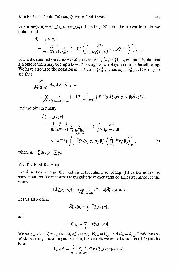
Effective Act ion for the Yukawa 2 Q u a n t u m Field Theory 445

where 6~(x;~)=,~Tp,,,(x")...6~p~(xl). Inserting (4) into the above formula we obtain that

A."_ ~, N(X; ~)

m ! k = t j = l oty) , ¢ = o ,

where the summation runs over all partitions {Ij}~= ~ of {1,..., m} into disjoint sets I~ (some of them may be empty). ( - 1) ~ is a sign which plays no role in the following. We have also used the notation m~ = [I~t, x j = {x~},~,~, and ~t~= {~f}~,~. It is easy to see that

6" ~(x; :t) A., ~(~ + ~3 I~ = 0

= X Z ( -1) ~ - p>m {131 . . . . . / S . - , . }

and we obtain finally

~.~- ~,N(X; ~)

m! E, 2 2 k= 1 {x~} {p~}{pj} p j >: " j

p~ (p - m) l I dp - "Y-~.P, N( x, Y; ~, [i)~(y; [~),

k

( -1) ~ I-I P/ j = 1 (p j-- m j)!

x I dp-"y j~l j = 1 r , ' , , , j Yj; % Pj) ~(Yj; I~j (5)

where m = y" m2, p = ~ pj.

IV. The First RG Step

In this section we start the analysis of the infinite set of Eqs. (III.5). Let us first fix some notation. To measure the magnitude of each term of (III.5) we introduce the n o r m

lI-~N(';~t)I1=sup ~ d"-'xlA~N(x;~x)J. {A} x t = O

Let us also define

and

g ~ ( x ) = E ~,~(x;~),

- " = I I A . , N ( " o O I t . I[a.,Nll E - " ,

We set gN.N(X_y)=g, ,~(x_y) , aN ,2 N---- ~ ,2 VN, N= V~N, and Y2N = (2~ ,. Undoing the Wick ordering and antisymmetrizing the kernels we write the action (ILl 3) in the form 4

AN, N(~) = E E ~ d"X-4~,N(X;~)v?(X;~). " = 0 ¢t A m

446

It is clear that

A. Lesniewski

t152,NII _-< C~, (1) --4 liAr, Nil < C4(1/N), (2)

uniformly in N and w. Performing the RG transformation we obtain the effective action AN_I,N(V~) which we write in the form

A N - 1 , N ( ~ ) ) = ~ 2 ~ m --m . ~ . d xAN_ 1, N(x, ~)~(x, ~). (3) m=O ~ Am

Proposition. The effective action (3) can be written as

AN- 1, N(CP) = ½1 dxdyg, s - 1, N(X -- y):~(x)lp(x): @(y)/p(y): -- f dxdudvdyCp(x)~p(x)~p(u)HN _ 1, N( x, u, v, y)~(v)~(y)~v(y) +VN-1,N+ E j'dmxA~-l,N(x;~x)~(x;et),

nl>--0,~

where the Wick ordering is performed with respect to SN- 1, and the kernels have the following properties:

_ m _ ~ m (i) For m>_8 we have AN_I,N--AN_I,~, and

IIh?v- 1,NIl <Bm(1/N) m/2- 1/£Nm/2+2"

(ii) Set Qm N( x -Y) = Tr{FN(x --Y)FN(Y --x)}, and 3 2, N = - Qm s(O), a 2 - 1, N = a2, N _~2N, N. Define gN_i,N(x--y;w) by (11.14) with a 2N,N replaced by C~N_I,N.2 Then gN- 1, N(x -- y) is given by

g,~- I,N(x-- y)= gN- I,N(x-- y) + gN-1,N * hN-1,N(x-- Y)

with

II hN- 1,NIl L' --< D(I/N) 2. (4)

Furthermore, we have the bound

4 ~ C4(1/N)3. IIAN-~,NII (5)

(iii) HN- 1,N(x, u, v, y)= gN- 1,N(X--U)FN(u-- v)gu- 1,N(v--y).

For the remainder m= 6 contributions we have

II A6- ~,Ntl ~ C6(1/N)3~c~I 1.

(iv) tIA2_ 1,N II < C2(1/N) 2.

(v) VN-1,N is equal to

- ½ rr {log(1 + w 4 _ 1, NG) - w 4 _ 1, NG) + E,,_ 1, N,

where

Furthermore,

EN- 1, N = EN,N -- ½ W f dxdyG(x - Y)QN,N(X-- Y)

[ A° - 1,N] ~ Co(1/N):JA[. (6)


The constants C, C i (j =0, 2, 4, 6) and D are independent of N andw. All the kernels are in H(f2N).

The rest of this section is devoted to the proof of the above proposition. We start with the easiest case of m > 8.

Estimating ][A~v_ 1,N[[, m ~ 8. Using (A.2) to bound the truncated correlation functions we obtain from (III.5)

1 k~ {~} 1 Cp_~c~_,,,,/2 l i a r - l , NIl< ~.. k.T E {xs}

p j > m j

× 2 PJ! I d x d y l ] 171~N(x,/,Ys)l r ~ : j=l (ps--mj)! .~,=o j = l

x exp { - xs£ar(X,, ..., Xk)}. (7)

Let us consider a single anchored tree T. Using translation invariance of A~v.N(x) and performing the integrations over the branches of Tin the order indicated by its tree structure we bound the corresponding integral by

k

Ck- *~:; ~(k-~) I1 llAf~ll. j = l

This and the fact that there are O(1)v-"k! anchored trees on {x~, ..., Xk} lead to the following bound on (7)

1

{I j} {p j} p j > m j

x ~ Pf l

s=l (p;- m;)!

E~ = ,~1 { I j } j = 1 =

Now, we have

C p - ml~(Np - m)/2 - 2 ( k - 1)

IIA~NII- (8)

m~ 5~ 1 ,

m l , . . . , m l ,u + ... + ', l = ,, 1-I mj!

j = l

where m;@0, j = 1, ..., I. This allows us to bound (8) by

' )} ~ -- ÷ 2 x E l-I E,. ~V~-2C"-~'tlA~NII ~N ~/2 {m j} j= 1 pj j

Using (1) and (2) we find that

E ~:~/:2-~cP'-'~'tf3f~NII <=O(1)O/N), mj>=O, p j > m j

and thus

IIAN-~,NII~2 ~ E E (C/N) k ~c; ~/2÷2 I = 1 {rnj}~ = 1

448 A. Lesniewski

Since the summation over k starts with m / 2 - 1 , the last inequality leads to

II Z?v_ 1, N ]1 _-< B"(1/N) m/2 - 1~, . /2 + 2

This completes the proof of (i). Now, the same brute force argument applied to m = 2, 4 would yield

I[ZI~c_I,NII < n2(l/N)tc~, -4 IIAN-1 NIt < B4(I/N).

These bounds are hopelessly non-iterative and a better analysis, including renormalization cancellations is required. It is a remarkable fact that only few low order terms have to be analysed carefully. The remaining terms play a less important role and all we need is to estimate them rather crudely. Extracting the new form-factor. From the first and second orders of the perturbation expansion we pick the following graphs:

where ~ represents the form-factor gN, N(x--Y), and - - stands for FN(x--y). In analytical terms, the above expression is equal to

gN, N( X - - Y) - - gN, N * QN, N * gN, N( X - - Y) " (9)

Observe that ON, u(P) is holomorphic for [Imput < (1 - r/)tc u, 0 < ~/< 1/2, and satisfies there

f~N, N(P)I--< C. (10)

Applying Cauchy's bound we obtain

[ON, N(P)-- ON,N(O)[ < Ct¢~ *[p[ , (11)

for ]Imp~[ <(1--2~/)xN. Repeating the argument leading to (I1.15) we find that

2 < - 1 IIQN, N * gN, N + 5~¢,NgIv, NtIL, = C~¢ .

This allows us to rewrite (9) as

gN, N(X-- y) + 2 CSN, ivgN, lV * gN, N(X -- y) + gN, N * hlv- l, ~v(x -- y),

where IIh~¢- ,,NIl = O(~cf¢ 1).

Lemma 1. The following equality holds:

gN- , , N ( x - y) = gN,tv * (~N,~ ~¢) J g~¢, N * . . . * gN, N(x - y ) . j = 0

Proof. We generate (13) by means of the obvious identity

_ A + m 2 + w o ~ 2 N = ( _ A 2 2 2 + m + WO~N_ I ,N) -~ W(~N,N,

(12)

(13)


and the fact that g,, N(x- y )= w ( - A + m2+ W0~n 2, N)-1( X --Y)" (13) converges, for by means of (II.15) and (10) we have

(5~,NYlIgN, N *...* gN, NI L~ j=O

E CJllgN,~ll~l=< ~ (C/N)/< ~ . Q.E.D. j = 0 j = 0

Comparing (12) with (13) and collecting the remainder terms we see that the new form-factor has the required form and (4) holds. Estimating IIA~-I,N[I- Let us break up (1II.5) into two parts: k<2 , and k>3 . Mimicking the proof of (i) we bound the second sum by C(1/N) 3. After extracting gN-1,N(x-Y) the first sum involves the following diagrams only:

where the dotted line stands for SN- 1. The norm of the first of them can be bounded as follows:

I dx2dx3dx41 IN( - x2)] lgN, N(x2 -- x31 Ir~(x3 - x,)t IgN, N(x4)l

< [[gN, N IlL111gN, NIIL2 IIFN]ILI IIFNI]L2 < C~c~ 1

Similarly, we bound the second graph by

dx2dx3dx4lgN, N(x2)l IFN(x2 -- x3)l IgN, N(x3 -- x4)l IFN(x4 -- x2)l

_-< IIgN,~IIL1 II gN, NIl L= IlrNII ~1 IlrNII ~= _-< c x ~ 1

The third graph can be bounded by

TrSN- 1(0) IIgN, NII~I [I FNII L1 ----< C~ff 1

This completes the proof of (5). Estimating [[A6_l,s[[. The only k = 2 contribution to A6_LN is the following graph:

Expanding gN, N in terms of gN- 1, N and shifting the remainder terms [which are O((1/N)3x~ 1)] into A 6_ 1,N we obtain the explicit form of the sixth order term in AN- 1, N(~). A6 - 1, N is a sum of the above mentioned remainder terms and the k > 3 part of (111.5). The latter can be easily bounded by O((1/N)3x~ 1). Estimating 2 IIAN_I,N[ I. After having exhibited the cancellation SN(0)--FN(0 ) = S~_ 1(0) we extract from (III.5) the following terms

- - t s ",~ +

450 A. Lesniewski

They can written as -g~_ 1,N(O)6(xl--x2) TrSs_ 1(0) and absorbed in the Wick ordering of the quartic term. Let us list the other graphs occurring in the first two orders of perturbation theory. They include:

. . . . . . . .

t ] • .¢

f /" \

Simple estimates show that all of these graphs are O(~c~"), for some q > 0. It remains to prove also that the k > 3 contribution to 2 lIAr- 1,NIl is O((1/N)2). Here some care is needed. As we have already observed, brute force estimation leads to a positive power ofxN in the bound for A~_ 1,N. A closer look at the Feynman graphs shows, however, that no such power should actually be present. Expanding in terms of Feynman graphs has the drawback that it destroys the combinatorial structure of the estimates and the convergence of (III.5) gets lost. Fortunately this is not necessary.

Let us collect all the terms in (III.5) which have the following structure

@ (14)

The sum of all such terms can be superficially bounded by C(1/N)ZxN, and we have to reduce the power of tc N by one. We write

where

r (x- y) = r l°)(x- y) + r 2 ) ( x - y),

M p2 + M 2 XN(P).

Using the fact that the determinant is a multilinear function of its columns we produce this way only 2 p - 1 terms in each order of k. Those terms which have at least one column of the F} 1) can already be bounded properly. The final remark of Appendix A shows that the power of xN in (A.2) drops by one. Repeating once more the estimates leading to (i) we bound the corresponding sum by 0((1/N)2).

Effective Action for the Yukawaz Quantum Field Theory 451

Potentially the most dangerous terms are those involving the Fs (°) propagators only. In the product

I] ~t~N(Xj, Yj,~j,~j) ~(Yj,~j j=l j=l ~)

in (III.5) we have pj = 2 or p~ = 4. The sum of terms where at least one factor with pj = 2 occurs can be bounded by O((1/N) 2) owing to (1). The sum of terms with all p ;=4, which is superficially O((1/N)3)KN, vanishes, as the following simple argument shows. We expand the correlation functions in terms of Feynman graphs. Since the number of vertices in ~N-~,N is odd, each Feynman graph contains an odd fermionic loop, say

Tr {~°)(x, - xz)r~°~(x~ - ~ ) . . . r~°~(~=- x 0}.

This is proportional to Tr (product of m 7-matrices)} = 0, for m is odd. To bound the other terms in A~_ ~,N we use the following formula

< ~'(x, uxl ; ~ u ~i)~(x~; ~t~)>~

= <~(X1 ; ~I)~(X~I ; ~tl) "''~.(X2 ; ~ 2 ) ' " ~ ( X k ; Qtk)>F T "T

K,,K2 \ j~K, /r K1uK2 ={2 ..... k} KinK2=0

x xl ;el) H ~(xj;%) , (15) ;eK2

which follows easily from (A.I). The number of terms on the RHS of(15) is bounded by C k which guarantees that (III.5) still converges. Let ~'(yluy~;l~xuIi'l) be the duster attached to ~v~(x0. Then it is either ~~(Y0~-p(Y'0~(Y'0 or ~(y~), and (15) generates the following types of terms:

(~)

@

(16)

Now it is an easy task to obtain the required bounds. To bound the terms of type (~) we notice that

II~N-~,N[I =<C, and hence

dxzdxadx4lFN(- x2)[ [gN, tc(X4)[ [~N- 1, N(X2 -- X3, X3 -- X41

---< It~N-1,NII II gN, N IIL31JrNIIL3~2< C~c~ 1/3"

452 A. Lesniewski

To bound the second type of terms in (15) we use the superficial bound on 5~:

113eN- 1,~t[ < C(1/N)~N,

and the following bound on ~- [cf. the discussion of (14)]:

119-~- .Nil < C(1/N) b,

where a + b >= 2. It follows that the terms of type (fl) can be bounded by C(I/N) z since the L 1-norm of the propagator between 5 a and ~- is O(~:ff 1). The proof of (iv) is complete. Vacuum energy. Proceeding as before we extract from (III.15) the following term

½gN-i,N(0) {TrSN_ 1(0)}21AI, and absorb it in the Wick ordering of the quartic term. To renormalize the logarithm occurring in VN, N we pick the following graphs:

- T +T "

We reintroduce now the bosonic cutoff as in Sect. II (to remove it in a moment again). We write

0~,~ = - ~,, ~ + (0~ ,~ + ~2,~)_ _ ~, ,~ + ~N,~,

and observe that

- Tr (gN, u; oQN, N) + wa2, N Tr (G0) + EN, N

= ~, , ~ Tr (g~, N; ~) + w ~ _ 1, ~ Vr (6~) + EN- 1,

- Tr {RN, N(gN.~-- wG)} + 0(~- 1).

Similarly, we have

Tr {(gN.,cQN, N) 2 }

= (6~, N) 2 Tr {g2, N} + Tr {(gu, NQN, 5/) 2 - - (gN, u 52, N)2} •

Lemma 2.

(i)

(ii)

(i)ITr{RN, N(gN, N--WG)}I<~Ctc~nIAI, 0 < q < l , 2 2 2 ITr{(gN, NQu, N) --(gN,NON, N) }1 < C~:ff IIAI,

uniformly in N, w, and A.

Lemma 3.

2 2 t 2 2 2 ITr {tog(1 + waN, NG~)-- 5N, NgN, N; ~ + ~(SN, N) gN, N;~

--log(1 + W~_ 1, NG0)} I < C(1/N)mIAI + O(Q- 1),

(17)

(18)

(19)

(20)

(21)

with C independent of N, w, and A.

Effective Action for the Yukawa z Quantum Field Theory 453

It follows from (17)-(21) that VN- 1,N is equal to

- ½ Tr {log(l 2 2 + waN- 1, NGo) -- WaN- 1, NG~} + EN- 1, N

+ O((1/N) 2) IAI + O(e - 1).

Removing the cutoff 0 as in Sect. II and shifting the remainder terms to A °_ 1, ~ we see that VN-1,N has the required form.

Proof of Lemma 2. (i) We have

ITr { RN, N(gN, N-- wG)}l < CIAI ~ dP[-gN, N(P)I I(gN, N-- wa) (p)[.

Using (11) we can bound the above expression by

C I A I N ~ 1 ~ dplpl (p2 + 1)- 2 < CIAl~cff " .

(ii) ITr{(gN, NQN, N)2 z 2 }t < CIAI 5 dplON, N(P) 2 -- (~N, N(0)2I (p2 + 1)- 2.

Using (10) and (11) we bound this expression by Ctc~*lAI. Q.E.D.

Proof of Lemma 3. It is easy to see that

log(1 + wa 2 ' NGe) = log0 + wa 2 - 1, NG~) -- log(1 -- 3 2, ugN, u; o) + O(e - ~).

Using the inequality

[Tr {log(1 + T ) - T+½ T2}[ _< Cll Tll 3 ,

valid for T e J 3 , we find that

LHS of (21) <=CllgN, NII~+O(o-a)<C(1/N)21AI+O(o-a). Q.E.D.

To complete the low order analysis of the vacuum energy we have to consider the graphs which we were ignoring so far. They include

!

and, as simple estimates show, are both O(K~ ~) [A[. Finally, let us consider the k > 3 part of(III.5). From each term of (III.5) we pick

a bosonic line and apply (15) to the ~'s attached to the line. Two kinds of terms are generated:

Both of them can clearly be bounded by O((I/N) 2) [A[. This proves (6). The analyticity statement follows from the fact that our expansions converge

uniformly in w. The proof of the proposition is complete.

454 A. Lesniewski

V. The General RG Iteration

The aim of this section is to prove the following theorem:

Theorem. Let n o and 1 be sufficiently large. For each n > n o the effective action A.,N(Cv) can be written in the form

a. , N(C;) = ½1 dxdyL , N(x - y) :CV(x)~(x): : qS(y)~(y):

- f dxdudvdy~(x)~(x)t~(u)H..~(x, u, v, y~(v)~O')~(y)

+V. ,N+ y, idmxA~,N(x;00~(x;a0, (1) m~0,~

where the Wick ordering is performed with respect to S.. There exist constants B, C i (0__<j < 6) and D, independent o f N and w such that the following statements hold:

(in) IlA.m, Nll~Bm(1/n)3+"(m-8)tCn m/2+2, m > 8 , where 0 < e < l / 1 2 is a f i x e d number.

(ii.) Set

Q.,N(x) = Tr F.(x)F,,(- x) + 2 y, F.(x)Fj{- x) . (2) j = n + l

Let 2 _ ~ . . N - O.,N(O), 2 2 2 . -- andc~n ,N=c~.+l .N- -b .+l ,N .Def ineg . ,N(x- -y ) tobe( I I .14)wi th o~ 2 replaced by 2 Then N , N O~n, N"

~., N(x - y) = g., N(x - y) + g., N * h., N(x - y) ,

with

[I h., N II L~ -< D(a/n). (3)

For the remainder terms we have the bound

!1A4. ~ II N C4(1/n) 2. (4)

N

(iii.) H.. N(x, u, v, y) = g., u(x - u) F. Fj{u - v)g., N(v- y). j = n + l

The remainder terms can be bounded as fol lows:

6 ]IA.,NII ~ C6(1/n)3lgn 1.

( iv,) 2 tlA,.NII < C 2 ( 1 / n ) .

(v.) l.~,,u is equal to

- ½ T r { l o g ( l +we2.,uG) - 2 wc%,NG} + E. ,u ,

where -- 1 E.. ~¢ - E . + 1. N - - ~ W I d x d y G ( x - y)Q. + L N( x - Y). Furthermore,

0 IZ., ~¢1 < Co(1/n)IAI. (5)

All the above listed kernels are in H(ON).

Remark. Notice that the bound (i.) is slightly worse than the corresponding bound of Sect. IV where we had e = 1/2.


Proofl The proof consists in showing that (in)--(Vn) imply (in_ 1)-(vn- 1). We write A.,e,~t~) in the form

A..N(~)= Z SdmxTt~N(X;~)~(X;~), (6) m>0,e~

with the obvious notation.

Lemma 1. There are constants ~1, or2>0 su'ch that

(tin<= 2 O~n, N ~ (72 n ,

uniformly in N.

Proof It is clear that

N 2 __ 2 ~ Y Tr{F~(x)Fk(-X)}(0) ~n, N -- O~n, n -- 2

j = l k = n + l

Since O(1)nN 2 ~.,. < O(1)n, it suffices to show that the second term is O(1). Indeed, it can be bounded by

~o

j = l k = n + l

=0(1) ~ P - " - ' ~ l-k<O(1). Q.E.D. j= l k=O

The lemma implies, by means of the same argument as in Sect. II, that

IIg.,NIIL.------ C(lln)'/~, (7)

uniformly in N. It follows that the kernels A.. ~" N, m = 2, 4, 6, of (6) obey the bounds

11.~6 s[i __< (~6(1/n)2t¢~- 1, (8)

IIA4,N[[ < C4(1/n), (9)

lIAr, NIL _-< C2, (10) uniformly in N. We can now pass to the estimates.

m >__ 8. We separate the term with k = 1, p = m (which is equal to A,m ~v) and write

- - m lm A._ ~,~(x) - A.. ~(x) + A._ 1,N(x) • (11)

Estimating liAr"-1,NJ[ proceeds in the same way as estimating []A~v-1,NlJ, We find easily that

{~k rain{re, k} (kl) (~pj KPJ/2-2CpJ .~p:i ~k-1 IIA21.Nll <2= t=lE . ,, . .u,,]

t x ~, ,~=1 G,s~,,s td"/2-2Cp'-"' 7Iv' ' . (12) {mJ}./=l "= n II n, NI I ) K n m / 2 + 2

Let us first consider the k = 1 contribution to (12). Using the induction hypothesis we find that

E l£pj2-2CPJ-mJ, ~vj.,N <B"~(1/n) 3+~(=~-8) , mi>=6 , (13) pj > mj

456 A. Lesniewski

We can thus bound the k = 1 term by

2raBm(1/r/)3 + am - s)x, ~- m/2 + Z.

TO bound the higher order contributions to (12) we use (13) and the following estimates [which easily follow from (8)-(10) and the induction hypothesis]:

LHS of(13) ~2C6(t/n) 2, mj=4, 5,

LHS of (13) <2C4(1/n), m ~ O .

Simple calculations using the assumption 0 < e < 1/12 show that the k = 2, 3 terms can be bounded by

4mBmc(1/n)3 + am- 8)tc n m/2 + 2

where C involves C4 and C6. A term with k > 4 can be bounded by

4mBmCk(1/n)3k/4 + e(m - 8) /~n m/2 + 2 .

Summing over k we obtain the following estimate on (12):

II h~_ 1, N I1 < 4mBmc( 1/n) 3 + am- 8)~C n m/2 + 2 .

It follows from (11) and (i.) that

II A~_ 1. NII < B"(1/(n - 1))3 +.(,.- s)x~-p/2 + 2,

provided that I has been taken large enough. This completes the proof of (i._ 1).

m=4. As in Sect. IV we extract from the first and second orders of the -4- perturbation expansion for A._ 1,N the following terms:

g.,N(x - y) - g.,N * Q.,N * g.,N( x - Y) (14)

(with the factor 1/2 in front). Observe that the cross-terms in Q.,N(x-y) come from the sixth order term in (1).

Lemma 2. O..,N(P) is holomorphic for tlmp.I < (1 -r/)t%, 0 < ~/< 1/2, and satisfies the inequalities:

I~.,N(P)I < C, (15)

I~..~¢(p)- (~.,N(0)I _-< C~;- llpl, Ilmp~,l < ( 1 - 2r/)c., (16)

uniformly in n and N.

Proof. Observe that

]Q..N(x)[<_Ct% ~ ~ je -~ lx l<~ C~:2exp(-x"[x[)' if tc.[x[___l, - - j=n+ 1 = ( C ~ . l x l - 1 if ~.lxl < 1.

This implies the analyticity statement and (15). Equation (16) follows from Cauchy's bound. Q.E.D.

Proceeding as in Sect. IV we write (14) as . 1 g~-t ,n(x--y)+g.-1 ,N h. - 1,N(x-y)


with I[h'.- x,NI[L 1 <D'(1/n) 2. Expanding gn, N in terms of g,_ 1,N and collecting the remainder terms we obtain

h,_ i, N(x) = h,, N(x) + h', _ 1, N(x) + O((1/n)2) .

Then tl h._ 1, Ntl L, < D ( n - 1)- 1, provided that D has been taken large enough. This proves (3).

To prove (4) we write again

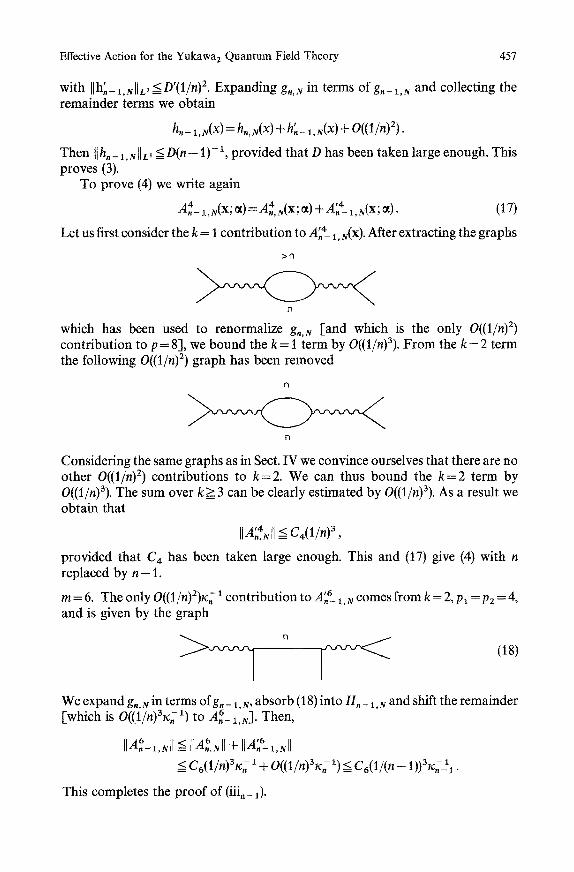
A . ' _ • " . 1, N( X, 0t) = An, N(X, a) + A; 41, ~(x; 0t). (17)

Let us first consider the k = 1 contribution to A~ 4_ i, u(x) • After extracting the graphs

> n

1"3

which has been used to renormalize g,,N [and which is the only O((1/n) 2) contribution to p = 8], we bound the k = t term by 0((1/n)3). From the k = 2 term the following O((1/n) 2) graph has been removed

n

1-1

Considering the same graphs as in Sect. IV we convince ourselves that there are no other O((1/n) 2) contributions to k=2 . We can thus bound the k = 2 term by 0((1/n)3). The sum over k ~ 3 can be clearly estimated by O(O/n)3). As a result we obtain that

IIA2N[I _-< C 4 ( 1 / n ) 3 ,

provided that C4 has been taken large enough. This and (17) give (4) with n replaced by n - 1 .

m = 6. The only O((1/n)2)tc2 1 contribution to A "6_ ~, N comes from k = 2, P l = P2 = 4, and is given by the graph

(18)

We expand g.,N in terms ofg._ 1,N, absorb (18) into H._ 1,u and shift the remainder [which is O((1/n)3~ 1) to A 6_ 1,N]. Then,

6 6 IIA.,Nll + [IA.-1,N/I < lIAr,6-1,NIl

< C6(1/n)3tc,~a + O((l/n)3tc~ 1)<= C6(1/( n _ 1))3/£n_11 .

This completes the proof of (iii n_ 1)-

458 A. Lesniewski

m = 2. We extract the same terms as above to absorb them in the Wick ordering of the quartic term. As in Sect. IV we verify that the low order contributions to k = 1, 2 are O(~:J). It remains to show that the remainder can be bounded by O((1/n)2), or in other words, we have to exhibit a mechanism allowing to reduce the power of x. by one.

Let us first consider the contributions to A'. ~_ 1,u which have the structure of : 2 (IV.14). In order not to complicate the notation we keep denoting them by A._ LN"

We claim that ,z A._ a. ~ can be written as

N - n + 1

Z B(.J)-I,N(X) (19) j = l

with

lIBeL 1,NIl £ C(1/n)2(1/l) j~ 1. (20)

Notice that (19) and (20) imply that ,2 [[A._l,u] [ <__C(1/n) 2. To prove the claim we proceed as follows. As in Sect. IV we write

= r . (o)+ r,(*),

and represent A~ z_ 1, N as

A,2_ 1.N(x)= 2(1) (1) A. _ l. N(x) + B. _ 1, N(X),

where a2{1) is the contribution containing no F. {*) propagators. Each term of Z ~ n - - l , N

B(.1)_1, N contains at least one column of the /~(1) propagators and can thus be bounded by O((1/n)2). Suppose we have represented ,2 A._ 1, N(X) as

BI/)-I.N(x), j = 0

where ~l._A2(m)l,N~.~!lv'~ contains no Q{1) propagators for j = n, ..., n + m - - 1 . We write

Fn+m-- F(O) _L r(1) - - ~ n +/ , t / / "t n + ~¢/ ~

and correspondingly

.~.P+,._ ~,N(X)-- ~P ~v~. ~,~10) ~"~" ~"P") LN(X) - - Z X n + m , N ~ , ~ ) ~ Z ~ - n + m - 1 , N ~ - " x ) ~ / X n + m -

= 2p(o) t x ~ . 2,p(1) ~..~ (21) - - ~ n + m - l , N ~ ] ~ X n + m - l , N l Y ' - . t ~

where ~',p(1) consists of terms containing at least one column of the Y.~+~ ~ X n + m - - l , N

propagators. Equation (21) induces the following decomposition ,~f A2(,.-~). ~ ~ x n - 1 , N •

A 2 ( m ) ( v ' ~ - - d 2 ( m + 1 ) [ v ~ ..1_ lt~(rn + 1 ) i v ] n - 1 , N k " ' ~ I - - ZJ-n - 1 , N ~,'a") ~ U n - 1 , N ~ ~ 1

where n(,.+ 1)tv~ consists of terms containing at least one column of the F.(~+)m a " n - - 1 , N I . A I

propagators. Since we gain one power of x~-+~,, in the bound for ~I.+,.,N~Aj,2'P(1) t-.~ we obtain that

B(,.+ 1) I < C(1/n)2(1/l) m n - I , N =

We set ...n(u-'+_ L N 1)=--a2(U-.+~ ~.- 1,N 1). By the same argument as in Sect. IV we have

n ( n N - n + 1 ) - L u It <C(1/n)2(1/l) ~ - ' .

This completes the proof of the claim.


For the terms which do not have the structure of (IV.14) we apply the following procedure. We choose an external leg of A "2_ 1,N(x) and write

N - n

A "~- 1,,,(x) = 2 C~ )- 1, N(x), j = 0

where C~ )_ 1,u(x) is the sum of contributions where the external leg touches a propagator F, +i for the first time. Applying (IV. 15) and proceeding as in Sect. IV we obtain that

N - n N - n IIA'.2-1,NII<C Y~ tcJ.j+C(1/n) 2 • l-J<C(1/n) 2,

j = O j = O

where the first contribution comes from the graphs of type (~), and the second comes from the graphs of type (/~).

Collecting all the contributions to A.Z_ 1,N we find finally that

IIA.Z- 1,NIl < C2(n- 1 + n - 2) < C 2 ( n - 1) -1 ,

provided C2 has been taken large enough. This completes the proof of (iv,_ 1).

m =0. The low order analysis is an almost word by word repetition of the analysis of Sect. IV. To bound the remainder terms we use the method explained above for the case of m = 2. Q.E.D.

As a simple corollary to the above theorem we obtain the stability bound. Set

Corollary.

Z A , N = (expAm u)s,, •

There exists C > 0 such that

uniformly in N.

Proof. We have

IZA,N[ <= e clAI ,

1ogZA,N = 0 V., N + A..N + log (exp A,,, N)s.. (22)

The first two summands can be bounded by CtAI. Indeed, for A°,~ we have (5), and V.,N can be bounded as follows

IV., ~r[ < ½ IWr {log(l + we. z, NG) -- we.z, NG}I + IE., NI

----¼tl 2 2 we.,NG II 2 + IE.,NI < C[AI.

To bound the third term on the RHS of(22) we use (A.2) with F. replaced by S.. The corresponding estimate is

f (x j ;~9 < c P + q Z e x p { - 0 - , ) M ~ ( x l . . . . . xk)}. j= 1 l Sn[ T e l

where C depends on n, 0 < t/< 1 is a certain number, and M is the fermionic mass. Using (i.)-(ivn) we find that

Ilog(expA.,N>sJ___<ClAI. Q.E.D.

460 A. Lesniewski

VI. The Continuum Limit and Borel Summabil i ty o f the Effective Action

In the previous section we have shown that A.,N stays bounded, when we go with n down to a scale no. We are now going to prove that the ultraviolet cutoff N can actually be removed, i.e. that the limit A . (~ ) - lira A.,N(~) exists for all n__> no.

N--~ oo Furthermore, we show that the perturbation expansion of A.(~) around w = 0 is Borel summable.

Observe that the N ~ limit of ~2,N is equal to

2 _ _ 2 T r { ~ ) } (0)+ Tr { ~ ) } (0), a n --

where S(x) is given by (II.3) with Z(P) = 1. This implies the existence of g . (x-y) . It is also easy to see that H.(x, u, v, y) and I1. exist. To prove that the other kernels in (V.1) have continuum limits we will investigate their behavior under a change of cutoff. Set

6A..N= A.,N + I-- A.,N.

The variations fiA.,N obey a recursion relation. We have

A._ 1,N+ 1(~) = log (expA.,N+ t(~ + ")>r.

= log (exp6A..N(~ +" ) expAn, N(~ + "))r . .

Subtracting A._ 1, N(~) = log <exp A., N(~ + )> r. from this equation and expanding in powers of A.,N and 6An,N we obtain that

bAn-I ,N(lP) = ~ ~ ((An, N(~+'))k(bA.,N(~+')) > r . , k=O l=1

or in terms of kernels

1 0° k(lX ~~ • - Z Z ( - 1 ) ~ 6A"-a,N(X'tX)-- m.t k~0 ~ 1 J~Y pj! . . :~ (~,~, ~p~ j : ~ (p j - m j)! • = t=l {~

pj >-- mj

k

x ~ dr-my H A.r~N(xj, Y j; ~j, IIj) 1 = 1

k + l

x • 6A~JN (x j, yfi %, [~j) j = k + l

J= r . " (1)

Proposit ion. We set #.,N= 116g,,NllL1. Suppose that I and no are large enough. Then there exist constants B, Cj (] = 0, 2, 4, 6), D and fl such that

( in) 116Anm,~ll <=B"#n,N(N/n)#(1/n)3+"(m-S)x2 ~/2+ z , m>=8.

(ii) [1OA,6 Nil <C6#n,N(N/n)P(I/n)ax; 1

(iiin) II 6hn, u II < D#n, N(N/n)P(1 In) 2 ,

[I 6A4, Ntl ~ C4#n, N(N/n)P( 1/n) 2"


(ivy) 1[3A2,NI[ <- C21tn, N(N/n)P(1/n).

(Vn) IOA°,NI < Co#.,N(N/n)P(1/n)]A[,

All the kernels are in H(f2N+ 1).

Proof The proof does not differ from the argument presented in Sect. V. We have to extract the same low order terms and make (essentially) the same estimates. Let us only comment on how to iterate the factor/t.,N(N/n) a which is crucial for the existence of the N ~ ~ limit. Observe the t6~.NI < C(~:,,/xN). This implies that

#.,N ~ C(1/n) (tc./~cN). (2)

The expansion

g . , ~ x ) = g . - 1 . N *

and (2) lead to the inequality

( - '~., NYg. - 1. N *-.- * g . - 1, N(x), j = 0

m,~, <_(1 + C/n)m_ 1,N. (3)

It is now easy to understand how the iteration goes for the terms with m > 6. For example, for m > 8 we have

gain- 1, N(x) ~--- 5A~ N(X) + 6A~ m_ 1, N(x),

where

[[ 6 A'."_ 1, u l[ <- 4"B"C#., N(N/n)t~( l /n) 3 + e.(m - 8)/~n m/2 + 2.

We prove (i n_ 1) by applying (3) and taking l large enough. Observe that the factor #., N(N/n) p is present in the bound for I] 6A2"_ 1,N I[ because the summation over I in (1) starts with l= 1. For the terms with m < 4 the iteration is slightly subtler. For example, for rn = 4 we have

[I 5an*-- 1,N[I =< C4#.,~N/n)~(l/n) 3 ,

and hence

tl fiA~_ 1, N]r ~_ C,,#,_ 1, N(N /n)~( 1 + C/n) (1/(n-- 1)) 2

<-- C4#, - ,, N(N/(n -- 1))P(1/(n -- l ))Z ,

provided that fl>= C. This explains the reason why the logarithmic correction (N/n) p has to be included in (i~)-(vn). Q.E.D.

It is now easy to show that A,(~) exists. We set

A~(x;~t)=A~,.(x;0t)+ ~ 3A~,(x;ot), m=>2, (4) j = n

and write analoguous formulae for h.(x) and A °. The series converges, since by means of the proposition and (2) we have that

j = n

462 A. Lesniewski

To prove that A~"(x; ~) has a Borel summable perturbation expansion in w we observe that for each test function f

IS d"xA~, j(x; 0t)f(x)[ < C(m, n)nf [[L~e-"J,

with C(m, n) and # independent ofj and w. The Bore1 summability of (4) follows now from the lemma of Appendix B.

Let us summarize the results of this section in the following theorem (below we change slightly the meaning of A~', 0 < m_< 6).

Theorem. The continuum limit action A.((v) exists and can be written in the following form:

A.(@ = ½ ~ dxdyg.(x- y) :VS(x)v?(x): :~(y)tp(y): + V.

+ X ~d"xA~(x;ct)~(x;~t), m > O , e x

where the Wick ordering is performed with respect to S.. All the kernels are in H(O) and they have Borel summable perturbation expansions around w = O. Furthermore, they satisfy the following bounds:

(i)

(ii)

(iii)

(iv)

llA~lt < Bm(l/n)3+~(m-s)~nm/Z+ 2, m> 8.

IlA~lt <Cm(l/n)Ztgn m/2+2 , m=4, 6.

IIA~ II --< C2(1/n),

IA°l _-< CoO~n)IAI.

Appendix A. Tree Decay of the Partially Truncated Correlation Functions

Let us recall the definition of partially truncated correlation functions. Suppose that the product ~'(xfi 0t j) contains pj fields of the ~ type and qj fields of the ~-type.

k

pj + qj is assumed to be even. Set j=l

<~(x; ~)>~: <~(X; ~)>r, (r = r.)

and define (j=I~l ~(xj;~t))~ inductively by

j = 1 {Kj}j = 1 j = 1 j l <<.m<_k

The summation in (1) extends over all partitions of {1, ...,k} into non-empty disjoint sets, and ( - 1)~ is the parity of a permutation which brings the fields ~'~(xj) on the RHS of (1) to the original order.

Let T be a graph on the points xl, ...,xp+q which is a tree with respect to the clusters x I .... ,x k. We call such a T an anchored tree on {xl,...,xk}. By A°r(xl, ..., Xk) we denote the length of T and by ~" the set of all anchored trees on { x , . . . ,

Effective Action for the Yukawa~ Quantum Field Theory 463

The following proposition gives a precise characterization of the decay

properties of ~(xi;~ . J

Proposition. There is a cons tant C such that

~(xj;e -<&+%c7 +q~/2 2 exp{--~c,~r(Xl,...,x~)}, (2) j = l T~ff"

where p = ~ p j , q = ~ q ~ .

Remarks . 1. Estimate (2) has been communicated to me by Gawedzki. Below I present a simple proof of (2) based on an expansion different from the one used by Gawedzki and Kupiainen [12].

2. Notice the good combinatorial properties of(2). The number of terms on the RHS of (2) is at most c v + q k !

This is because of the fermionic character of the correlation functions. An analogous bound for bosonic correlation functions would involve the combinatorial factor of p! (where 2p is the number of fields).

We turn to the proof of (2). The untruncated correlation function

(~Ij=l "~(Xj;~J))F can be explicitly written (up to a sign which will not bother us)as

the determinant detJg, where the entries of J/{ are given by

j , j ' = 1 . . . . . k, i = 1 . . . . . p j, i ' = 1 . . . . , q j,. Introducing Grassmann variables qj, i, flj.i we can write d e t J / ( u p to a sign) as the Berezin integral

k pj qj f I~ l] d~/~,~ ~ dF/j,,exp(~l,~¢ll). (3)

j = l i = 1 "=

We present V=(fl, d¢I!) as a "two-body potential":

v= 2 1 <=i,j<=k ~,j

where llj=(~/~, 1, ...,qj, p), fli=(~]j,1 .... ,(/~,q). For each pair (i,j) we introduce an interpolating parameter 0__< sij <= I, s~ = sj~, and set

k

V(s)= 2 v.+ y s, V j. (4) i = 1 i*j

We call (4) a BF (----Battle-Federbush) decoupling of V if there is a bijective mapping g: {1 .... ,k}~{1 ..... k} with g(1)=1 such that

sg(i)gv) = sisi + 1... s j_ 1, i < j , (5)

where 0 < sj < 1,j = 1,..., k - 1. The following lemma is an immediate consequence of (3) and [18, 19].

464 A. Lesniewski

Lemlna 1. The partially truncated part o f d e t J g is given by

~, ~d'qdfl I] (Vij+ Vj~)SdpT(s)expV(s), (6) T e ..q-~. ( i, j ) e T

where ~-~ is the set of trees on k vertices and dPT(S) is a probability measure concentrated on such s that V(s) is a BF decoupling of V.

Let us now consider a single term on the RHS of (6). Expanding the product t ] (V/j+ Vi, i) we represent it as a sum of terms of the form

( i , j ) e T

(a product of k - 1 propagators, each of which joins two different k - 1

xj's)× l~I f/i,..,#j,.,., I ] rl').m~qi,..,. (7) t = 1 / = a + l

Observe that if #i,, and tb, m are factors in (7) then all the terms in V(s) involving these variables are actually absent. The Berezin integral may be this factored and evaluated to obtain a product of k - 1 propagators multiplied by a ((p + q)/2 - k + 1) × ((p + q)/2 - k + 1) determinant. Using (III. 1) we can bound the first factor by

k - l . k - 1 C ~. exp { - ~.SFT(Xl, .... X~)), (8)

where T is an anchored tree on {xl . . . . , xk}. The entries of the determinant have the structure s~jF.~,.aj,..(x~,.-xj, m). We wish to show that the determinant can be written as a Gramm determinant det {(fa, gb)}, provided that s is in the support of dp~(s).

Lemma 2. There exist unit vectors e l , . . . , ek ~ lR k such that (e i, ej) =sij, with ( . , ) the usual scalar product in I~ k.

Lemma 3. There exist A , ( x - . ), B a ( y - . )~ L2OR2)GL2(]R2) such that F~,a(x- y) = (A~(x--) , B a ( y - . )). Moreover, IIA~(x - " )1[, tIB~( x - " )I[ < Cx~/2, uniformly in x.

These two lemmata imply that

s~iF~,. .~j,,.(x~..- y j..3 = (ei®A~,,.,(xi,.--"), e~®Btjj.~(y~.m-- )),

for s in the support of dpr(s). Using Gramm's inequality

ldet{(f~,gb)}l < I] IILtl Ilgbll a

we can bound our determinant by C p ÷ qx~ p + q)/ 2 - k + ~. This and (8) lead immediately to (2).

Proof of Lemma 2. Let s~i have the form (5). By v~ we denote the i-th unit vector (v~)j = 6i~- We set el = Vx and define eg~j) inductively by

eg~j)=sj_leg(j_l)+(1--s2_l)l/2vj, j = 2 ..... k - l .

Then

ile.<j)ll 2 2 2 2


and

(%(o, ego)) = si- 1 (eo(0, eo(J- 1)) = s~...s j_ zs j - 1

=s~j, for i < j . Q.E.D.

Proof of Lemma 3. The following argument is due to Feldman et al. [13]. We set

2

I'~, tj(x --)7) = Z ~ d2 tA~, ~(x - t)Ba,,(y - t), 1:=1

with J(p) = ( - ilk + M ) (pC + M z) - 3/4X(p)l/2 ' ~(p) = (p2 + M2) - 1/4 x Z(p)l/zl , where X(P) is given by 01.6). This gives the required representation, The bounds IIA~(x- " )ll, IIB~(x-" )II < C~,/2 follow by a simple calculation. Q.E.D.

Remark. If in b columns of de t Jg the propagators F ( x - y ) are replaced by the propagators

1 M F ( ° ) ( x - y) = ( ~ ) 2 ~ dp p2 + M 2 Z(P) elp(~-r) ,

then the power of ~. in (2) is reduced by b, This follows from the fact that

IF~ff)(x- Y)I < Ce - ~,1~- rl

and IIa~°)(x - ")1[, IIn~°)(x - )1[ <C.

Appendix B. A Lemma on Borel Summability

A well known criterion of Borel summability of a divergent power series is the following theorem 1-20, p. 192]:

Theorem (Watson). Let f ( z ) be holomorphic in

D e-- {z: Izl < r, largzl < 7r/2 + e},

where r > O, and 0 < e < 7r/2 are certain numbers, and continuous in D,. Suppose that

k

f ( z ) = ~ ajz j + Rk(z), j = 0

and that there exist C, cr > 0 such that

[a,l < Cakk ! , (1)

IRe(z)l < Ca e + X(k + I)! lzt k + 1 (2)

uniformly in k and z ~ D~. Define

® tk ( B f ) ( t ) = Z ak in"

k=O

The function (B f ) ( t ) is hoIomorphic in {t: jargtj <e} and

f ( z ) = ~ d te -*(Bf ) ( t z ) , 0

for [z[ < r, [argz[ < e.

466 A. Lesniewski

In the lemma which we prove below we deal with a special situation which we encounter in our analysis of the Yukawa model. The sets g2j have the same meaning as in Sect. IV.

Lemma. Let f~(z), j = n, n + 1 .... be a sequence of functions such that

(i) f i sH(Q j),

(ii) [ fj(z)l < Ce-"J, /~ > 0, (3)

with C independent of z and j. Then the function

f ( z )= ~ f~(z) (4) j=n

satisfies the assumptions of Watson's theorem with D, = f2.

Proof. It follows from (3) that (4) converges uniformly in O. This implies the analyticity statement. For each j we write

k f j(Z) = 2 "(J)'rm-I- l'~(J)(q'~ 7. ~ o ~.,. . . . . k w , O j , (5)

m = O

where

1 d" a~)- m! d f i fj(z)[~ = o.

It follows from Cauchy's bound and (3) that

[a~)[ __< C e - Mr f m = C Cr~ e - #j '

where C? 1 =jrj. Let us bound the remainder term in (5). If [zl < ½rj, then

R~J)(z) = ~ a~)z m, m = k + l

and we have

[R~j)(z)[ <= 2CC~+ lju+ 1 e - UJlzlk + , .

For z E f2 with Iz[ > ½rj we make a direct estimate

k

IRL~)(z)I ~ Ifj(z)l + Z m = O

k + l

<= 2ce-"j Z m = O

Now, we write

[a~)l lzlm < Ce- UJ ( l + m~o (lz[/r j)m)

m k + l k + l /tj k + l ([zl/rj) <4CC~ j e - I z l •

where

a k

k f(z) = Z a,, zm + Rk(Z),

m = O

a~ ), Rk(Z)= ~ R~)(z). j=n j=n

(6)

(7)

(8)


It follows from (6) that

lakl < CC] ~ fie-uJ<= CC ] ~ dttke-ut= (C/p)(C1/#)kk!. j=n 0

Similarly, (7) and (8) imply that

lRk(Z)l<(4C/p)(Cl/l~)k+l(k+l)!lzl k+l , zef2.

The last two inequalities imply (1) and (2), respectively, if we replace 4C/# by C and C1/# by a. Q.E.D.

Acknowledgements. I would like to thank Konrad Osterwalder for numerous invaluable discussions and encouragement. My thanks are also due to Jiirg Fr6htich, Krzysztof Gawedzki, and Sandy Rutherford for very helpful discussions.

References

1. Glimm, J., Jaffe, A.: Self adjointness of the Yukawa2 Hamiltonian. Ann. Phys. 60,.321 (1970) 2. Gtimm, J., Jaffe, A.: The Yukawa2 quantum field theory without cutoffs. J. Funct. Anal. 7, 323

(1971) 3. Schrader, R.: A Yukawa quantum field theory in two spacetime dimensions without cutoffs.

Ann. Phys. 70, 412 (1972) 4. Osterwalder, K., Schrader, R.: Euclidean fermi fields and a Feynman-Kac formula for boson-

fermion models. Helv. Phys. Acta 46, 277 (1973) 5. Seller, E.: Schwinger functions for the Yukawa model in two dimensions with space-time

cutoff. Commun. Math. Phys. 42, 163 (1975) 6. Seiler, E., Simon, B.: Commun. Math. Phys. 45, 99 (1975) 7. McBryan, O.: Volume dependence of Schwinger functions in the Yukawa2 quantum field

theory. Commun. Math. Phys. 45, 279 (1975) 8. Cooper, A., Rosen, L.: The weakly coupled Yukawa z field theory: cluster expansion and

Wightman axioms. Trans. Am. Math. Soc. 234, 1 (1977) 9. Magnen, J., S6n6or, R.: The Wightman axioms for the weakly coupled Yukawa model in two

dimensions. Commun. Math. Phys. 51, 297 (1976) I0. Renouard, P.: Analyticit6 et sommabilit6 "de Boret" des fonctions de Schwinger du mod+le de

Yukawa en dimension d=z, I. and II. Ann. l'Inst. H. Poincar6 27, 237 (1977); 31, 235 (1979) 11. Balaban, T., Gawedzki, K.: A low temperature expansion for the pseudoscalar Yukawa model

of quantum fields in two space-time dimensions. Ann. l'Inst. H. Poincar6 36, 271 (1982) 12. Gawedzki, K., Kupiainen, A.: Commun. Math. Phys. 102, 1 (1985) 13. Feldman, J., Magnen, J., Rivasseau, V., S6n~or, R.: A renormalizable field theory: the massive

Gross-Neven model in two dimensions. Commun. Math. Phys. 103, 67 (1986) 14. Wilson, K., Kogut, J.: The renormalization group and the e expansion. Phys. Rep. 12C, 75

(1974) 15. Gawedzki, K., Kupiainen, A.: Les Hunches Lectures (1984) 16. Gallavotti, G.: Rev. Mod. Phys. 57, 471 (1985) 17. Caianello, E.: Nuovo Cimento 3, 223 (1956) 18. Battle, G., Federbush, P.: Ann. Phys. 142, 95 (1982) 19. Brydges, D.: Les Houches Lectures (1984) 20. Hardy, G.: Divergent series. London: Oxford University Press 1949

Communicated by A. Jaffe

Received June 24, 1986

Effective action for the Yukawa 2

Documents

Transcript of Effective action for the Yukawa 2