Effect Sizes and Power Analyses - School of...

Effect Sizes and Power Analyses

Nathaniel E. Helwig

Assistant Professor of Psychology and StatisticsUniversity of Minnesota (Twin Cities)

Updated 04-Jan-2017

Nathaniel E. Helwig (U of Minnesota) Effect Sizes and Power Analyses Updated 04-Jan-2017 : Slide 1

Copyright

Copyright © 2017 by Nathaniel E. Helwig


Outline of Notes

1) Effect Sizes:Definition and OverviewCorrelation ES FamilySome ExamplesDifference ES FamilySome Examples

2) Power Analyses:Definition and OverviewOne sample t testTwo sample t testOne-Way ANOVAMultiple regression


Effect Sizes

Effect Sizes


Effect Sizes Definition and Overview

What is an Effect Size?

An effect size (ES) measures the strength of some phenomenon:Correlation coefficientRegression slope coefficientDifference between means

ES are related to statistical tests, and are crucial forPower analyses (see later slides)Sample size planning (needed for grants)Meta-analyses (which combine ES from many studies)



Population versus Sample Effect Sizes

Like many other concepts in statistics, we distinguish between ES inthe population versus ES in a given sample of data:

Correlation: ρ versus rRegression: β versus β

Mean Difference: (µ1 − µ2) versus (x1 − x2)

Typically reserve Greek letter for population parameters (ES) andRoman letter (or Greek-hat) to denote sample estimates.



Effect Sizes versus Test Statistics

Sample ES measures are related to (but distinct from) test statistics.ES measures strength of relationshipTS provides evidence against H0

Unlike test statistics, measures of ES are not directly related tosignificance (α) levels or null hypotheses.



Standardized versus Unstandardized Effect Sizes

Standardized ES are unit freeCorrelation coefficientStandardized regression coefficientCohen’s d

Unstandardized ES depend on unit of measurementCovarianceRegression coefficient (unstandardized)Mean difference


Effect Sizes Correlation Effect Size Family

Overview of Correlation Effect Size Family

Measures of ES having to do with how much variation can beexplained in a response variable Y by a predictor variable X .

Some examples of correlation ES include:Correlation coefficientR2 and Adjusted R2

η2 and ω2 (friends of R2 and R2a)

Cohen’s f 2



Correlation Coefficient

Given a sample of observations (xi , yi) for i ∈ {1, . . . ,n}, Pearson’sproduct-moment correlation coefficient is defined as

rxy =sxy

sxsy=

∑ni=1(xi − x)(yi − y)√∑n

i=1(xi − x)2√∑n

i=1(yi − y)2

wheresxy =

∑ni=1(xi−x)(yi−y)

n−1 is sample covariance between xi and yi

s2x =

∑ni=1(xi−x)2

n−1 is sample variance of xi

s2y =

∑ni=1(yi−y)2

n−1 is sample variance of yi

Measures strength of linear relationship between X and Y .



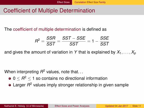
Coefficient of Multiple Determination

The coefficient of multiple determination is defined as

R2 =SSRSST

=SST − SSE

SST= 1− SSE

SST

and gives the amount of variation in Y that is explained by X1, . . . ,Xp

When interpreting R2 values, note that. . .0 ≤ R2 ≤ 1 so contains no directional informationLarger R2 values imply stronger relationship in given sample



Adjusted Coefficient of Multiple Determination (R2a)

The adjusted R2 is a relative measure of fit:

R2a = 1− SSE/dfE

SST/dfT= 1− σ2

s2Y

where s2Y =

∑ni=1(yi−y)2

n−1 is the sample estimate of the variance of Y .

Note that R2 = 1− σ2/s2Y where

σ2 = SSE/n is MLE of error variances2

Y = SST/n is MLE of variance of Yso R2

a replaces the biased estimates σ2 and s2Y with the unbiased

estimates σ2 and s2Y in definition of R2.



ANOVA Coefficient of Determination (η2 and η2k )

In the ANOVA literature, R2 is typically denoted using

η2 =SSRSST

which is the amount of variation in Y attributable to group membership.

Also could consider partial η2 for k -th factor

η2k =

SSRk

SST

which is the proportion of variance in Y that can be explained by thek -th factor after controlling for the remaining factors.



Calculating η2k in R (Balanced ANOVAs)

R’s aov function does not calculate this, but you can (easily) write yourown function for this using output of anova function:

eta.sq <- function(mod,k=NULL){atab = anova(mod)if(is.null(k)){ k = 1:(nrow(atab)-1) }sum(atab[k,2]) / sum(atab[,2])

}

This function is only appropriate for balanced multiway ANOVAs.



Adjusted ANOVA Coefficient of Determination (ω2)

Note that η2 suffers from the same over-fitting issues as R2:If you add more groups, you will have higher η2

For a one-way ANOVA we could adjust η2 as follows

ω2 =SSB − dfBSSW/dfW

SST + SSW/dfW

where SSB and SSW are the SS Between and Within groups.Note that ω2 is less biased estimate of population η2



Calculating ω2 in R (One-Way ANOVA)

R’s aov function does not calculate this, but you can (easily) write yourown function for this using output of anova function:

omega.sq <- function(mod){atab = anova(mod)ssb = atab[["Sum Sq"]][1]ssw = atab[["Sum Sq"]][2]dfb = atab[["Df"]][1]msw = atab[["Mean Sq"]][2](ssb - dfb*msw) / (ssb + ssw + msw)

}



Cohen’s f 2 Measure

Jacob Cohen’s f 2 measure is defined as

f 2 =X 2

1− X 2

where X 2 is some R2-like measure.

Can define f 2 using any measure we’ve discussed so far:

Regression: f 2 = R2

1−R2

ANOVA: f 2 = η2

1−η2

Note that f 2 increases as R2 (or η2) increases.



Cohen’s f 2 Measure for “Hierarchical” Regression1

Suppose we have a regression model with two sets of predictors:A: contains predictors we want to control for (i.e., condition on)B: contains predictors we want to test for

Suppose there are q predictors in set A and p − q predictors in set B.Model A: yi = b0 +

∑qj=1 bjxij + ei

Model AB: yi = b0 +∑p

j=1 bjxij + ei

Can use a version of Cohen’s f 2 to examine contribution of B given A:

f 2B|A =

R2AB − R2

A

1− R2AB

1Note that this has nothing to do with hierarchical linear models (multilevel models).


Effect Sizes Some Examples

Example 1: One-Way ANOVA

> set.seed(1)> g = factor(sample(c(1,2,3),100,replace=TRUE))> e = rnorm(100)> mu = rbind(c(0,0.05,0.1),c(0,0.5,1),c(0,5,10))> eta = omega = rep(NA,3)> for(k in 1:3){+ y = 2 + mu[k,g] + e+ mod = lm(y~g)+ eta[k] = summary(mod)$r.squared+ omega[k] = omega.sq(mod)+ }> eta[1] 0.03222293 0.22131646 0.94945042> omega[1] 0.01214756 0.20362648 0.94791418



Example 2: Two-Way ANOVA

> A = factor(rep(c("male","female"),each=12))> B = factor(rep(c("a","b","c"),8))> set.seed(1)> e = rnorm(24)> muA = c(0,2)> muB = c(0,1,2)> y = 2 + muA[A] + muB[B] + e> mod = aov(y~A+B)> eta.sq(mod)[1] 0.6710947> eta.sq(mod,k=1)[1] 0.4723673> eta.sq(mod,k=2)[1] 0.1987273



Example 3: Simple Regression

> set.seed(1)> x = rnorm(100)> e = rnorm(100)> bs = c(0.05,0.5,5)> R = Ra = rep(NA,3)> for(k in 1:3){+ y = 2 + bs[k]*x + e+ smod = summary(lm(y~x))+ R[k] = smod$r.squared+ Ra[k] = smod$adj.r.squared+ }> R[1] 0.002101513 0.179579589 0.956469774> Ra[1] -0.008081125 0.171207952 0.956025588



Example 4: Multiple Regression (GPA Data)

> gpa = read.csv(paste(myfilepath,"sat.csv",sep=""),header=TRUE)>> g1mod = lm(univ_GPA~high_GPA,data=gpa)> Rsq1 = summary(g1mod)$r.squared> g2mod = lm(univ_GPA~high_GPA+math_SAT,data=gpa)> Rsq2 = summary(g2mod)$r.squared> (Rsq2-Rsq1)/(1-Rsq2) # f^2 (math_SAT given high_GPA)[1] 0.02610875>> g1mod = lm(univ_GPA~math_SAT,data=gpa)> Rsq1 = summary(g1mod)$r.squared> g2mod = lm(univ_GPA~math_SAT+high_GPA,data=gpa)> Rsq2 = summary(g2mod)$r.squared> (Rsq2-Rsq1)/(1-Rsq2) # f^2 (high_GPA given math_SAT)[1] 0.4666959


Effect Sizes Difference Effect Size Family

Overview of Difference Effect Size Family

Measures of ES having to do with how different various quantities are.For two population means

θ =µ1 − µ2

σ

measures standardized difference, where σ is standard deviation.

Some examples of difference ES include:Glass’s ∆

Cohen’s dHedges’s g and g∗

Root mean square standardized effect (RMSSE)



Gene Glass’s ∆ (1976)

If group 1 is the “control” group and group 2 is the “test” group use:

∆ =x1 − x2

s1

where s1 is sample standard deviation of control group.

Glass, G.V. (1976). Primary, secondary, and meta-analysis of research.Educational Researcher, 5, 3–8.



Jacob Cohen’s d (1969)

When xi1 ∼ (µ1, σ2) and xi2 ∼ (µ2, σ

2) we can use

d =x1 − x2

sp

where sp ={

(n1−1)s21+(n2−1)s2

2n1+n2

}1/2is MLE of the standard deviation σ

and s2j =

∑nji=1(xij − xj)

2/(nj − 1) is the sample standard deviation.

Cohen, J. (1969). Statistical power analysis of the behavioral sciences. SanDiego, CA: Academic Press.



Larry Hedges’s g

Hedges’s g modifies the denominator of Cohen’s d

g =x1 − x2

s∗p

where s∗p ={

(n1−1)s21+(n2−1)s2

2n1+n2−2

}1/2is an unbiased estimate of σ.

Hedges, L.V. (1981). Distribution theory for Glass’s estimator of effect sizeand related estimators. Journal of Educational Statistics, 6, 107–128.



Larry Hedges’s g∗

It can be shown that E(g) = δ/c(n1 + n2 − 2) where

δ =µ1 − µ2

σand c(m) =

Γ(m/2)√m2 Γ

(m−12

)is a term that depends on the sample size.

Hedges’s g∗ corrects the bias of g by multiplying it by c(n1 + n2 − 2):

g∗ = c(n1 + n2 − 2)g

Hedges, L.V. (1981). Distribution theory for Glass’s estimator of effect sizeand related estimators. Journal of Educational Statistics, 6, 107–128.



Mean Difference Effect Sizes in R

diffES <-function(x,y,type=c("gs","g","d","D")){md = mean(x) - mean(y)nx = length(x)ny = length(y)if(type[1]=="gs"){m = nx + ny - 2cm = gamma(m/2)/(sqrt(m/2)*gamma((m-1)/2))spsq = ((nx-1)*sd(x)+(ny-1)*sd(y))/mtheta = cm*md/sqrt(spsq)

} else if(type[1]=="g"){spsq = ((nx-1)*sd(x)+(ny-1)*sd(y))/(nx+ny-2)theta = md/sqrt(spsq)

} else if(type[1]=="d"){spsq = ((nx-1)*sd(x)+(ny-1)*sd(y))/(nx+ny)theta = md/sqrt(spsq)

} else { theta = md/sd(x) }}



Root Mean Square Standardized Effect (RMSSE)

In one-way ANOVA we can use the RMSSE:

Ψ =

√1

k−1∑k

j=1(µj − µ)2

σ2 =

√√√√ 1k − 1

k∑j=1

δ2j

whereµj is j-th group’s population meanµ is overall population meanσ2 is common varianceδj =

µj−µσ is j-th group’s standardized population difference



Mean Difference Effect Sizes in R (continued)

RMSSE function for one-way ANOVA model:

rmsse <- function(x,g){mx = tapply(x,g,mean)ng = nlevels(g)nx = length(x)msd = sum((mx-mean(x))^2)/(ng-1)mse = sum((mx[g]-x)^2)/(nx-ng)sqrt(msd/mse)

}



Example 5: Student’s t test

> set.seed(1)> e = rnorm(100)> mu = rbind(c(0,0.05),c(0,0.5),c(0,1))> gs = g = d = D = rep(NA,3)> for(k in 1:3){+ x = rnorm(100,mean=mu[k,1])+ y = rnorm(100,mean=mu[k,2])+ gs[k] = diffES(x,y)+ g[k] = diffES(x,y,type="g")+ d[k] = diffES(x,y,type="d")+ D[k] = diffES(x,y,type="D")+ }> rtab = rbind(gs,g,d,D)> rownames(rtab) = c("gs","g","d","D")> colnames(rtab) = c("small","medium","large")> rtab

small medium largegs -0.1172665 -0.3922036 -0.8320117g -0.1177130 -0.3936971 -0.8351799d -0.1183060 -0.3956804 -0.8393874D -0.1226476 -0.4126996 -0.8745153



Example 6: One-Way ANOVA (revisited)

> set.seed(1)> g = factor(sample(c(1,2,3),100,replace=TRUE))> e = rnorm(100)> mu = rbind(c(0,0.05,0.1),c(0,0.5,1),c(0,5,10))> rvec = rep(NA,3)> for(k in 1:3){+ y = 2 + mu[k,g] + e+ rvec[k] = rmsse(y,g)+ }> rvec[1] 0.2348609 0.6844976 5.4882692


Power Analyses

Power Analyses


Power Analyses Definition and Overview

Some Classification Lingo

Classification Outcomes Table:Is Negative Is Positive

Test Negative True Negative False NegativeTest Positive False Positive True Positive

Some vocabulary:Sensitivity = TP / ( TP + FN ) =⇒ True Positive RateSpecificity = TN / ( TN + FP ) =⇒ True Negative RateFall-Out = FP / ( FP + TN ) =⇒ False Positive RateMiss Rate = FN / ( FN + TP ) =⇒ False Negative Rate



NHST and Statistical Power

NHST Outcomes Table:H0 True H1 True

Accept H0 True Negative Type II ErrorReject H0 Type I Error True Positive

Note: Type I = False Positive, Type II = False Negative

α = P(Reject H0 | H0 true) = P(Type I Error)

β = P(Accept H0 | H1 true) = P(Type II Error)

power = P(Reject H0 | H1 true) = 1− β



Visualizing Alpha, Beta, and Power

−4 −2 0 2 4 6

0.0

0.1

0.2

0.3

0.4

1 − β = 0.64

x

f(x)

α = 0.05β = 0.36

α

β 1 − β

H0 H1



Things that Affect Power

Power is influenced by three factors:Population effect size (larger ES = more power)Precision of estimate (more precision = more power)Significance level α (larger α = more power)

Note: you can control two of these three (precision and α)

Precision of the estimate is controlled by the sample size n.Larger n gives you more precision (more power)Power analysis can give you needed n to find effect



Alpha, Beta, and Power: Mean Differences

−4 −2 0 2 4

0.0

0.1

0.2

0.3

0.4

1 − β = 0.13

x

f(x)

α = 0.05β = 0.87

−4 −2 0 2 40.

00.

10.

20.

30.

4

1 − β = 0.26

x

f(x)

α = 0.05β = 0.74

−4 −2 0 2 4

0.0

0.1

0.2

0.3

0.4

1 − β = 0.44

x

f(x)

α = 0.05β = 0.56

−4 −2 0 2 4 6

0.0

0.1

0.2

0.3

0.4

1 − β = 0.64

x

f(x)

α = 0.05β = 0.36

−4 −2 0 2 4 6

0.0

0.1

0.2

0.3

0.4

1 − β = 0.8

x

f(x)

α = 0.05β = 0.2

−4 −2 0 2 4 60.

00.

10.

20.

30.

4

1 − β = 0.91

x

f(x)

α = 0.05β = 0.09



Alpha, Beta, and Power: SD Differences

−4 −2 0 2 4

0.0

0.1

0.2

0.3

0.4

1 − β = 0.26

x

f(x)

α = 0.05β = 0.74

−2 0 2 40.

00.

20.

4

1 − β = 0.41

x

f(x)

α = 0.05β = 0.59

−2 −1 0 1 2 3

0.0

0.2

0.4

0.6

1 − β = 0.53

x

f(x)

α = 0.05β = 0.47

−2 −1 0 1 2 3

0.0

0.2

0.4

0.6

0.8

1 − β = 0.64

x

f(x)

α = 0.05β = 0.36

−2 −1 0 1 2 3

0.0

0.2

0.4

0.6

0.8

1 − β = 0.72

x

f(x)

α = 0.05β = 0.28

−2 −1 0 1 2 30.

00.

20.

40.

60.

81.

0

1 − β = 0.79

x

f(x)

α = 0.05β = 0.21



Alpha, Beta, and Power: Alpha Differences

−4 −2 0 2 4 6

0.0

0.1

0.2

0.3

0.4

1 − β = 0.37

x

f(x)

α = 0.01β = 0.63

−4 −2 0 2 4 60.

00.

10.

20.

30.

4

1 − β = 0.48

x

f(x)

α = 0.02β = 0.52

−4 −2 0 2 4 6

0.0

0.1

0.2

0.3

0.4

1 − β = 0.64

x

f(x)

α = 0.05β = 0.36

−4 −2 0 2 4 6

0.0

0.1

0.2

0.3

0.4

1 − β = 0.76

x

f(x)

α = 0.1β = 0.24

−4 −2 0 2 4 6

0.0

0.1

0.2

0.3

0.4

1 − β = 0.83

x

f(x)

α = 0.15β = 0.17

−4 −2 0 2 4 60.

00.

10.

20.

30.

4

1 − β = 0.88

x

f(x)

α = 0.2β = 0.12



Alpha, Beta, and Power: R code

plotpower <- function(m0,m1,sd=1,alpha=0.05){x0seq = seq(m0-3*sd,m0+3*sd,length=500)x1seq = seq(m1-3*sd,m1+3*sd,length=500)cval = qnorm(1-alpha,m0,sd)power = round(pnorm(cval,m1,sd,lower=F),2)plot(x0seq,dnorm(x0seq,m0,sd),xlim=c(m0-3*sd-1,m1+3*sd+1),type="l",

lwd=2,xlab=expression(italic(x)),ylab=expression(italic(f(x))),main=bquote(1-beta==.(power)),cex.main=2,cex.axis=1.25,cex.lab=1.5)

lines(x1seq,dnorm(x1seq,m1,sd),lwd=2)px=c(rep(cval,2),seq(cval-0.01,m1-3*sd,length=50),m1-3*sd,cval)py=c(0,dnorm(cval,m1,sd),dnorm(seq(cval-0.01,m1-3*sd,length=50),m1,sd),

rep(dnorm(m1-3*sd,m1,sd),2))polygon(px,py,col="lightblue",border=NA)px=c(rep(cval,2),seq(cval+0.1,m0+3*sd,length=50),m0+3*sd,cval)py=c(0,dnorm(cval,m0,sd),dnorm(seq(cval+0.1,m0+3*sd,length=50),m0,sd),

rep(dnorm(m0+3*sd,m0,sd),2))polygon(px,py,col="pink",border=NA)legend("topleft",legend=c(as.expression(bquote(alpha==.(alpha))),

as.expression(bquote(beta==.(1-power)))),fill=c("pink","lightblue"),bty="n")

}


Power Analyses One Sample t Test

One Sample Location Problem

Suppose we have sample of data xiiid∼ N(µ, σ2) and we want to make

inferences about the mean µ.

Letting x = 1n∑n

i=1 xi denote the sample mean, we have

E(x) = E

(1n

n∑i=1

xi

)=

1n

E

(n∑

i=1

xi

)=

1n

n∑i=1

E(xi) =nµn

= µ

V (x) = V

(1n

n∑i=1

xi

)=

1n2 V

(n∑

i=1

xi

)=

1n2

n∑i=1

V (xi) =nσ2

n2 =σ2

n

where E(x) and V (x) are the expectation and variance of x .

Implies that x ∼ N(µ, σ2/n)



One Sample t Test Statistic

Suppose we want to test one the of the following sets of hypothesesH0 : µ = µ0 versus H1 : µ > µ0

H0 : µ = µ0 versus H1 : µ < µ0

H0 : µ = µ0 versus H1 : µ 6= µ0

and define δ = µ1 − µ0 where µ1 is the true mean under H1.

Our t test statistic has the form: T = δσ/√

n

δ = x − µ0

σ2 = 1n−1

∑ni=1(xi − x)2



Power Calculations for One Sample t Test

Given the test statistic T = δσ/√

n , power is influenced by

Effect size δPrecision σ/

√n

Significance level α

Note that there are four parameters that affect power: {δ, σ, n, α}

If you know 3 of 4 (and desired power), you can solve for fourthThe power.t.test function in R does this for you



One Sample t Test Power in R (one-sided)

> power.t.test(n=NULL,delta=-1,sd=1,sig.level=0.05,power=0.80,+ type="one.sample",alternative="one.sided")Error in uniroot(function(n) eval(p.body) - power, c(2, 1e+07),tol = tol, : no sign change found in 1000 iterations

> power.t.test(n=NULL,delta=1,sd=1,sig.level=0.05,power=0.80,+ type="one.sample",alternative="one.sided")

One-sample t test power calculation

n = 7.727622delta = 1

sd = 1sig.level = 0.05

power = 0.8alternative = one.sided



One Sample t Test Power in R (two-sided)

> power.t.test(n=NULL,delta=1,sd=1,sig.level=0.05,power=0.80,+ type="one.sample",alternative="two.sided")


n = 9.937864delta = 1


power = 0.8alternative = two.sided



One Sample t Test Power in R (small effect size)

> power.t.test(n=NULL,delta=0.2,sd=1,sig.level=0.05,power=0.80,+ type="one.sample",alternative="two.sided")


n = 198.1513delta = 0.2





One Sample t Test Power in R (really small effect size)

> power.t.test(n=NULL,delta=0.02,sd=1,sig.level=0.05,power=0.80,+ type="one.sample",alternative="two.sided")


n = 19624.12delta = 0.02




Power Analyses Two Sample t Test

Two Sample Location Problem

Suppose we have two independent samples of data xi1iid∼ N(µ1, σ

2)

and xi2iid∼ N(µ2, σ

2) and we want to make inferences about δ = µ1−µ2.

Letting x1 = 1n1

∑n1i=1 xi1 and x2 = 1

n2

∑n2i=1 xi2, we have

E(x1) = µ1 and E(x2) = µ2

V (x1) =σ2

n1and V (x2) =

σ2

n2

where E(·) and V (·) are the expectation and variance operators.

Implies that x1 ∼ N(µ1, σ2/n1) and x2 ∼ N(µ2, σ

2/n2).Note that x1 − x2 ∼ N(δ, σ2

∗) where σ2∗ = σ2( 1

n1+ 1

n2)



Two Sample t Test Statistic

Suppose we want to test one the of the following sets of hypothesesH0 : δ = 0 versus H1 : δ > 0H0 : δ = 0 versus H1 : δ < 0H0 : δ = 0 versus H1 : δ 6= 0

where δ = µ1 − µ2 is the population mean difference.

Our t test statistic has the form: T = δ

σ√

1n1

+ 1n2

δ = x1 − x2

σ2 =(n1−1)s2

1+(n2−1)s22

n1+n2−2 is the pooled variance estimate

s21 = 1

n1−1∑n1

i=1(xi1 − x1)2 and s22 = 1

n2−1∑n2

i=1(xi2 − x2)2



Power Calculations for Two Sample t Test

Given the test statistic T = δ

σ√

1n1

+ 1n2

, power is influenced by

Effect size δPrecision σ

√1n1

+ 1n2

= σ√

2/n if n1 = n2 = n


Note that the same four parameters affect power: {δ, σ, n, α}

If you know 3 of 4 (and desired power), you can solve for fourthThe power.t.test function in R does this for you



Two Sample t Test Power in R (one-sided)

> power.t.test(n=NULL,delta=-1,sd=1,sig.level=0.05,power=0.80,+ alternative="one.sided")Error in uniroot(function(n) eval(p.body) - power, c(2, 1e+07),tol = tol, : no sign change found in 1000 iterations

> power.t.test(n=NULL,delta=1,sd=1,sig.level=0.05,power=0.80,+ alternative="one.sided")

Two-sample t test power calculation

n = 13.09777delta = 1


power = 0.8alternative = one.sided

NOTE: n is number in *each* group



Two Sample t Test Power in R (two-sided)

> power.t.test(n=NULL,delta=1,sd=1,sig.level=0.05,power=0.80,+ alternative="two.sided")


n = 16.71477delta = 1






Two Sample t Test Power in R (small effect size)

> power.t.test(n=NULL,delta=0.2,sd=1,sig.level=0.05,power=0.80,+ alternative="two.sided")


n = 393.4067delta = 0.2






Two Sample t Test Power in R (really small effect size)

> power.t.test(n=NULL,delta=0.02,sd=1,sig.level=0.05,power=0.80,+ alternative="two.sided")


n = 39245.36delta = 0.02





Power Analyses One-Way Analysis of Variance

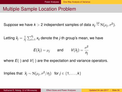
Multiple Sample Location Problem

Suppose we have k > 2 independent samples of data xijiid∼ N(µj , σ

2).

Letting xj = 1nj

∑nji=1 xij denote the j-th group’s mean, we have

E(xj) = µj and V (xj) =σ2

nj

where E(·) and V (·) are the expectation and variance operators.

Implies that xj ∼ N(µj , σ2/nj) for j ∈ {1, . . . , k}



One-Way ANOVA F Test Statistic

Suppose we want to test the overall (omnibus) F testH0 : µj = µ ∀j versus H1 : not all µj are equal

where µ is some common population mean.

Our F test statistic has the form: F = MSBMSW =

1k−1

∑kj=1 nj (yj−y)2

1n−k

∑kj=1

∑nji=1(yij−yj )2

If nj = n ∀j , then F = nΨ2 where Ψ is estimated RMSSE

Ψ2 = V (between)

V (within)is ratio of variances

MSW = σ2 is the pooled variance estimate



Power Calculations for One-Way ANOVA

Given the test statistic F = nΨ2, power is influenced byEffect sizes δj = yj − yPrecisions σ and nSignificance level α

Note that there are four parameters that affect power: {V (δ), σ,n, α}

If you know 3 of 4 (and desired power), you can solve for fourthThe power.anova.test function in R does this for you



One-Way ANOVA Power in R (large effect size)

> power.anova.test(groups=3,n=NULL,between.var=1,within.var=2,+ sig.level=0.05,power=0.80)

Balanced one-way analysis of variance power calculation

groups = 3n = 10.69938

between.var = 1within.var = 2sig.level = 0.05

power = 0.8

NOTE: n is number in each group



One-Way ANOVA Power in R (medium effect size)



groups = 3n = 20.30205


power = 0.8




One-Way ANOVA Power in R (small effect size)



groups = 3n = 482.7344


power = 0.8




One-Way ANOVA Power in R (really small effect size)



groups = 3n = 4818.343


power = 0.8



Power Analyses Multiple Regression

Multiple Regression Problem

Suppose we have a multiple linear regression

yi = b0 +

p∑j=1

bjxij + ei

for i ∈ {1, . . . ,n} whereyi ∈ R is the real-valued response for the i-th observationb0 ∈ R is the regression interceptbj ∈ R is the j-th predictor’s regression slopexij ∈ R is the j-th predictor for the i-th observation

eiiid∼ N(0, σ2) is a Gaussian error term



Multiple Regression F Test Statistic

Suppose we want to test the overall (omnibus) F testH0 : b1 = · · · = bp = 0 versus H1 : not all bj equal 0

where the bj terms are the unknown population slopes.

Our F test statistic has the form: F = MSRMSE =

1p∑n

i=1(yi−y)2

1n−(p+1)

∑ni=1(yi−yi )2

Reminder: f 2 = R2

1−R2 = SSR/SST1−SSR/SST = SSR

SSE

Note that f 2 =(

pn−(p+1)

)F



Power Calculations for Multiple Regression

Given the test statistic F =(

n−(p+1)p

)f 2, power is influenced by

Effect sizes f 2

Degrees of freedom p and n − (p + 1)


Note that there are four parameters that affect power: {f 2,p,n, α}

If you know 3 of 4 (and desired power), you can solve for fourthSee pwr.f2.test function in pwr R package



Multiple Regression Power in R (large effect size)

Assume that p = 2 and R2 = 0.8, so that our ES is f 2 = 4.

> library(pwr)> pwr.f2.test(u=2,v=NULL,f2=4,sig.level=0.05,power=0.80)

Multiple regression power calculation

u = 2v = 3.478466

f2 = 4sig.level = 0.05

power = 0.8

Need n = dve+ (p + 1) = 4 + 3 = 7 subjects.



Multiple Regression Power in R (medium effect size)

Assume that p = 2 and R2 = 0.5, so that our ES is f 2 = 1.

> pwr.f2.test(u=2,v=NULL,f2=1,sig.level=0.05,power=0.80)


u = 2v = 10.14429

f2 = 1sig.level = 0.05

power = 0.8




Multiple Regression Power in R (small effect size)

Assume that p = 2 and R2 = 0.1, so that our ES is f 2 ≈ 0.11.

> pwr.f2.test(u=2,v=NULL,f2=0.11,sig.level=0.05,power=0.80)


u = 2v = 87.65198

f2 = 0.11sig.level = 0.05

power = 0.8




Multiple Regression Power in R (really small ES)




u = 2v = 963.4709

f2 = 0.01sig.level = 0.05

power = 0.8




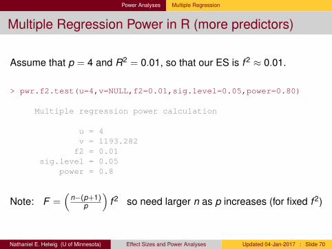
Multiple Regression Power in R (more predictors)




u = 4v = 1193.282

f2 = 0.01sig.level = 0.05

power = 0.8

Note: F =(

n−(p+1)p

)f 2 so need larger n as p increases (for fixed f 2)


Effect Sizes and Power Analyses - School of...

Documents

Transcript of Effect Sizes and Power Analyses - School of...