EFFECT OF URBAN PLANNING ON URBAN GROWTH PATTERN: A …
74
EFFECT OF URBAN PLANNING ON URBAN GROWTH PATTERN: A CASE STUDY OF SHENZHEN YAYUAN LEI February, 2019 SUPERVISORS: Dr. N. Schwarz Dr. J. Flacke
Transcript of EFFECT OF URBAN PLANNING ON URBAN GROWTH PATTERN: A …

EFFECT OF URBAN PLANNING ON URBAN GROWTH PATTERN: A CASE STUDY OF SHENZHEN
YAYUAN LEI February, 2019
SUPERVISORS: Dr. N. Schwarz Dr. J. Flacke


Thesis submitted to the Faculty of Geo-Information Science and Earth Observation of the University of Twente in partial fulfilment of the requirements for the degree of Master of Science in Geo-information Science and Earth Observation. Specialization: Urban Planning and Management SUPERVISORS: Dr. N. Schwarz Dr. J. Flacke THESIS ASSESSMENT BOARD: Prof. dr. R. V. Sliuzas (Chair) Dr. M. Netzband (External Examiner, University of Wuerzburg)
EFFECT OF URBAN PLANNING ON URBAN GROWTH PATTERN: A CASE STUDY OF SHENZHEN
YAYUAN LEI Enschede, The Netherlands, February, 2019

DISCLAIMER This document describes work undertaken as part of a programme of study at the Faculty of Geo-Information Science and Earth Observation of the University of Twente. All views and opinions expressed therein remain the sole responsibility of the author, and do not necessarily represent those of the Faculty.

i
ABSTRACT
It is essential to understand how urban plans affect urban growth patterns in order to improve current urban planning and management systems. Few studies have been conducted to analyse the urban growth patterns of Shenzhen, an international megacity located in southern China, but none of them revealed the relationships between urban planning and urban growth patterns. This study aims to explore the effects of master plans on urban growth patterns in different plan time periods in Shenzhen. The study employed three different methods to identify urban growth patterns of Shenzhen in 1988-1999, 1999-2011 and 2011-2015 based on the land cover data. The urban growth patterns in this study were identified as infilling, expansion and outlying by Landscape Expansion Index (LEI) at patch level and as infilling, expansion, isolated, clustered branch and linear branch by the method developed by Wilson et al. (2003) at pixel level. In addition, LEI was broken into LEI 4-cell method and LEI 8-cell method based on the neighbourhood rules they are following to define a patch. The results from three methods are different: Wilson’s method detected a higher percentage of outlying pattern in all of the three periods; LEI 4-cell and LEI 8-cell detected a higher percentage of expansion in 1988-1999 and 1999-2011 but a higher percentage of infilling in 2011-2015. Through reviewing the master plans of Shenzhen and relevant literature, potential factors influencing urban growth patterns have been selected. After checking the data availability, the planned built-up zone, planned ecological protection zone, planned main road and planned highway in master plan 1996-2010 and 2010-2020 were considered as potential urban planning factors affecting urban growth patterns. In order to have an insight on how the urban planning factors influenced the urban growth patterns in Shenzhen, the relationships between urban growth patterns identified by three methods and urban planning factors were checked in multinomial logistic regression models. The regression models, which considered classified urban growth patterns by LEI 4-cell method as dependent variable, perform well as they have prediction accuracy of 71% and 74%, respectively, in 1999-2011 and 2011-2015. The model results indicate that the planned main road in Master Plan of Shenzhen 1996-2010 and the planned built-up zone in the Master Plan of Shenzhen 2010-2020 had effects on urban growth patterns but less contribution than most of the other selected factors, e.g. distance to ocean. Compared to that, the regression models for the urban growth patterns identified by the LEI 8-cell method have less explained variance. The drawback of Wilson’s method is distinguishing some linear urban growth from clustered urban growth in this case study. This study concludes that the LEI 4-cell method is capable of detecting the infilling, expansion and outlying patterns in Shenzhen and the multinomial regression model can differentiate these patterns based on the urban planning, socio-economic, proximity, accessibility and neighbourhood data. The urban planners in Shenzhen could make use of the effects of planned main road and planned built-up zone on urban growth patterns to guide the urban development of this city. Key words: Urbanisation, Urban Growth Pattern, Urban Planning, Multinomial Logistic Regression, Shenzhen

ii
ACKNOWLEDGEMENTS
First of all, I would like to express my sincere gratitude to my supervisors Dr N. Schwarz and Dr J. Flacke. I received a lot of valuable guidance and suggestions from them whenever I got problems or had questions about my thesis. I also received great encouragement from them when I felt unconfident in the thesis process. Without them, the thesis cannot be completed on time. I would like to thank all my lovely classmates in UPM for their enthusiastic encouragement and willingness to help when I came across problems. I am also grateful to Dr. P. Dou and Urban Planning and Land Resources Commission of Shenzhen Municipality for their data provision. I would like to thank ITC Excellence Scholarship Programme for providing me with the generous financial support. It made it possible for me to complete my MSc course in ITC. Lastly, I would like to express my deep gratitude to my parents for their love and continuous encouragement throughout this MSc research.

iii
TABLE OF CONTENTS List of Figures ............................................................................................................................................................... iv List of Tables .................................................................................................................................................................. v
Introduction ........................................................................................................................................................... 1 1.1. Background and Justification ....................................................................................................................................1 1.2. Research Problem ........................................................................................................................................................2 1.3. Research Objectives and Research Questions .......................................................................................................3 1.4. Thesis Structure ...........................................................................................................................................................3
Literature Review .................................................................................................................................................. 5 2.1. Urban Growth Pattern ...............................................................................................................................................5 2.2. Urban Growth Pattern Identification Method .......................................................................................................6 2.3. Urban Planning in China and Specifically Shenzhen ............................................................................................7 2.4. Influential Factors of Urban Growth ................................................................................................................... 11 2.5. Logistic Regression .................................................................................................................................................. 14
Data and Methodology ..................................................................................................................................... 15 3.1. Study Area .................................................................................................................................................................. 15 3.2. Data Description and Processing .......................................................................................................................... 15
3.2.1. Land Cover Data ............................................................................................................................................ 15 3.2.2. Data for Factors Influencing Urban Growth Pattern ............................................................................. 17
3.3. Methodology ............................................................................................................................................................. 23 3.3.1. Urban Growth Pattern Identification Using Method Developed by Wilson et al. ............................ 24 3.3.2. Urban Growth Pattern Identification by Computing Landscape Expansion Index ......................... 27 3.3.3. Multinomial Logistic Regression Model .................................................................................................... 28
Results and Discussion ..................................................................................................................................... 33 4.1. Urban Growth of Shenzhen ................................................................................................................................... 33 4.2. Urban Growth Patterns of Shenzhen ................................................................................................................... 34 4.3. Comparison of Multinomial Logistic Regression Modelling Outputs ............................................................ 39
4.3.1. Multicollinearity Test ..................................................................................................................................... 39 4.3.2. Modelling Outputs Comparison ................................................................................................................. 40 4.3.3. Spatial Autocorrelation Test ........................................................................................................................ 44
4.4. Relationships between Urban Growth Pattern and Its Determinants ............................................................ 45 4.4.1. Relationships between Urban Growth Pattern and Urban Planning Factors ..................................... 46 4.4.2. Relationships between Urban Growth Pattern and Socio-economic, Physical, Accessibility,
Proximity and Neighbourhood Influential Factors ................................................................................. 48 4.5. Reflection on the Data, Methodology of the Case Study .................................................................................. 49
Conclusions......................................................................................................................................................... 53 List of References ....................................................................................................................................................... 55 Appendix ...................................................................................................................................................................... 59

iv
LIST OF FIGURES
Figure 2-1 Land use plan in the Master Plan of Shenzhen SEZ (1986-2000) ..................................................... 8 Figure 2-2 Urban structure plan in Master Plan of Shenzhen SEZ (1986-2000) ................................................ 9 Figure 2-3 Urban structure plan in Master Plan of Shenzhen (1996-2010) ....................................................... 10 Figure 2-4 Urban structure plan in Master Plan of Shenzhen (2010-2020) ....................................................... 10 Figure 3-1 The geographical location of Shenzhen ............................................................................................... 15 Figure 3-2 The processing of acquired land cover data ........................................................................................ 16 Figure 3-3 The area of corrected urban lands of Shenzhen ................................................................................ 17 Figure 3-4 Influential factor maps-I ......................................................................................................................... 20 Figure 3-5 Influential factor maps-II ....................................................................................................................... 21 Figure 3-6 Influential factor maps-III ...................................................................................................................... 22 Figure 3-7 Influential factor maps-IV ...................................................................................................................... 23 Figure 3-8 Flowchart of overall methodology (every colour refers to one objective: orange-objective 1,
blue-objective 2, purple-objective 3) ............................................................................................................... 24 Figure 3-9 Process of urban growth pattern classification using Wilson's method (source: Wilson et al.,
2003) ..................................................................................................................................................................... 26 Figure 3-10 Three types of urban growth pattern (source: Liu et al., 2010) ...................................................... 27 Figure 3-11 Distributions of samples for spatial logistic regression ................................................................... 30 Figure 4-1 Urban growth from 1988 to 2015 in Shenzhen .................................................................................. 33 Figure 4-2 The percentage of the area of the urban growth patterns in the three planning periods ............. 35 Figure 4-3 Examples of urban growth patterns of Shenzhen from 1999 to 2011 using three different
methods ............................................................................................................................................................... 35 Figure 4-4 Maps of urban growth patterns in Shenzhen identified by LEI 4-cell method in the three plan
periods .................................................................................................................................................................. 37 Figure 4-5 Maps of urban growth patterns in Shenzhen identified by LEI 8-cell method in the three plan
periods .................................................................................................................................................................. 38 Figure 4-6 Maps of urban growth patterns in Shenzhen identified by Wilson’s method in the three plan
periods .................................................................................................................................................................. 38 Figure 4-7 Example of problematic identification of urban growth patterns in 1999-2011 in Shenzhen by
Wilson's method ................................................................................................................................................. 39

v
LIST OF TABLES
Table 2-1 Rationales of selected potential influential factors .............................................................................. 13 Table 3-1 The areas of original urban and corrected urban in Shenzhen ......................................................... 16 Table 3-2 Data availability of the selected potential influential factors ............................................................. 18 Table 3-3 Identification of pixel category in the method of Wilson et al. ......................................................... 25 Table 3-4 Identification of urban growth patterns in the method of Wilson et al. ......................................... 25 Table 3-5 Outlying pattern classification rules within each clump ..................................................................... 26 Table 3-6 Assumptions about the effects of urban planning factors on urban growth patterns .................. 28 Table 4-1 Urban growth and urban growth rate of Shenzhen in the three plan periods................................ 34 Table 4-2 Percentage of the area of three outlying patterns classified by Wilson's method in the three
planning periods ................................................................................................................................................ 36 Table 4-3 Multicollinearity diagnosis of predictors ............................................................................................... 39 Table 4-4 Parameters of overall qualities of the multinomial logistic regression models in 1999-2011 ....... 40 Table 4-5 Parameters of overall qualities of the multinomial logistic regression models in 2011-2015 ....... 41 Table 4-6 Parameter estimates of the three multinomial logistic regression models in 1999-2011 .............. 43 Table 4-7 Parameter estimates of the three multinomial logistic regression models in 2011-2015 .............. 44 Table 4-8 Results of spatial autocorrelation test on model residuals by calculating Moran’s I ..................... 45


EFFECT OF URBAN PLANNING ON URBAN GROWTH PATTERN: A CASE STUDY OF SHEZNHEN
1
INTRODUCTION
Many countries are experiencing rapid urban growth. The location and intensity of growth in urban areas can have negative impacts on both ecological and social systems (Hepinstall-Cymerman, Coe, & Hutyra, 2013). In order to manage and control the negative effects, planners and policymakers have applied planning and policy approaches to guide the locations and intensity of urban development. However, for informing or improving the future planning and policy approach, it is important to evaluate if the desired urban growth patterns have been reached when the regulations aiming to guide the urban growth are present.
1.1. Background and Justification Urbanization is defined as the physical growth of urban areas which is a consequence of people migrating from rural to urban areas (Bhatta, 2010). More than half of the world population has settled in urban areas by 2008 and this figure will increase to 60% by 2030 (United Nations, 2014). As a consequence, the worldwide observed urban area is increasing correspondingly. By 2030, the urban land cover will increase to 1.2 million km2 which is nearly triple of the urban land in 2000 (Seto, Güneralp, & Hutyra, 2012). Even though urbanization brings ample economic and technological benefits (Runde, 2015), its impact on ecology is devastating. It not only hinders the natural ecological boundaries but also hampers the agricultural fields (Huang, Xia, Xiao, & He, 2017). Not only the growing amount of urban land has threatened the well-being of the cities, but also the pattern of urban growth has affected the cities largely. Although urban growth has been widely discussed, its definition is still not clear. While some researchers refer to it as a change in population or economic performance, for some it is related to the spatial expansion of urban areas (Reis, Silva, & Pinho, 2016). In this study, the focus will be set on the spatial dimension of urban growth. Urban growth pattern is defined as the characteristic of spatial changes that happen in metropolitan areas (Aguilera, Valenzuela, & Botequilha-Leitão, 2011). Those urban growth patterns perceived as negative have an irreversible impact on the sustainability of the environment and human (Bhatta, 2010). For example, the leapfrogging urban growth will contribute to the increase in travel demand that raises energy consumption. On the other hand, the smart urban growth patterns, such as infilling growth, devote themselves to compact the urban areas and reduce energy consumption (Transportation Research Board and National Research Council, 2009). Therefore, figuring out the urban growth patterns is very important for urban planners who are aiming at a more sustainable urban growth. The planning and policy methods, such as spatial zoning and urban growth boundaries, are widely used to mitigate the negative urban growth patterns. For example, urban growth boundaries are set to encourage urban development inside urban growth boundaries and reduce the leapfrogging developments in this way (Millward, 2006). Understanding how the urban planning approaches function on the urban growth patterns is essential to improve the current urban planning system and management of the urban lands. China is under urbanisation in an unprecedented rate which led to the probably greatest human-settlement in the history (Bai, Shi, & Liu, 2014). Shenzhen, a fast-growing city, is located on the southeast coast of China. Shenzhen was promoted as a city in 1979 and the first Chinese Special Economic Zone (SEZ) was established in Shenzhen in 1980. Special Economic Zones refer to the geographic regions within a country

EFFECT OF URBAN PLANNING ON URBAN GROWTH PATTERN: A CASE STUDY OF SHEZNHEN
2
which have more liberal laws and economic policies than the other regions to encourage foreign investment (Wang, 2013). After the establishment of SEZ, Shenzhen has developed from a small city of about 300,000 inhabitants to a megacity with approximately 15 million people by 2015 (UN-Habitat, 2015). In order to accommodate the increased population, the urban land increased from 5.6% to 41.8% of the whole city
(Dou & Chen, 2017). In the past, the urban land cover of Shenzhen expanded dramatically, especially at the city fringe, due to the continuously growing informal peri-urban settlements (Sumari, Shao, Huang, Sanga, & Van Genderen, 2017). Following this, issues like agricultural land loss, traffic congestion and air pollution were registered. In response to these issues, urban planning (e.g. Spatial zoning), recognised as an important tool to regulate the urban growth (Long, Gu, & Han, 2012), was frequently employed by the Shenzhen’s urban planning department (Deng, Fu, & Sun, 2018). Since this department of Shenzhen is planning to compile a new urban master plan 2020-2030 for Shenzhen to encourage sustainable urban development (Urban Planning and Land Resources Commission of Shenzhen Municipality, 2017a), there is a need to reflect the effects of urban planning on urban growth patterns for the forthcoming urban plan making.
1.2. Research Problem Urban growth patterns are studied widely with different perspectives in different countries. Some scholars claim that these patterns are closely related to the local urban plans. Liu et al. (2010) monitored the dynamic land changes in China in the early 21st century and explored the relations between land use changes and land management policies. They found that the conversion from natural resources and cropland to urban land has decreased since the implementation of the policies for protecting natural resources and agriculture. Osman, Arima and Divigalpitiya (2016) measured the patterns of urban sprawl in the Greater Cairo Metropolitan Region by building a geospatial indicators system and GIS spatial analysis methods. The results indicate that the conspicuous fragmentation and unevenness of landscape patterns were caused by the poor implementation of land use planning. Regarding urban planning and urban growth patterns, there have been very few researches done in Shenzhen. Lv, Wu, Wei, Sun and Wen (2009) distinguished three urban growth patterns (i.e. infilling, edge-expansion, and outlying) in Shenzhen based on remote sensing images. They found that outlying was the main pattern during 1979 and 2005 in Shenzhen, the amount and the spatial distributions of urban growth patterns varied in different counties and different time phases. However, they did not explain the reasons behind the variations. Li et al. (2005) discovered that from 1978 to 1999, a large amount of cultivated land in Shenzhen converted to urban built-up areas and the newly built-up areas at first fragmented, then expanded and finally amalgamated. They also argued that the changes in urban landscape patterns were the consequences of both urban planning and disordered human disturbances (e.g. economic activities). But it needs more evidence from the analysis on the relevant data. Dou and Chen (2017) determined that the extensional urbanisation is the main urban growth pattern in Shenzhen from 1988 to 2015 by monitoring the landscape change using satellite images. According to them, the extensional growth patterns were probably caused by foreign capital investment and government policies of introducing satellite towns and industrial parks. In short, these studies made good contributions to the understanding of the urban growth patterns of Shenzhen but the relationship between urban planning and urban growth patterns requires further studies. Given that three master plans have been implemented in Shenzhen and are recognised as “significant directors” of the development of Shenzhen (Urban Planning and Land Resources Commission of Shenzhen Municipality, 2017b). Therefore, the aim of this study is to understand the urban growth patterns in Shenzhen over time and their relationship with urban plans in three master plan periods in Shenzhen.

EFFECT OF URBAN PLANNING ON URBAN GROWTH PATTERN: A CASE STUDY OF SHEZNHEN
3
1.3. Research Objectives and Research Questions The general objective is to understand the effects of urban planning on urban growth patterns in different time periods in Shenzhen. The sub-objectives and related research questions are designed as follows: 1. To identify the historical urban growth patterns in Shenzhen.
a) How did the urban area grow over time during the master plan periods? b) What were the urban growth patterns in Shenzhen during the master plan periods?
2. To identify the influential factors of urban growth patterns in different time periods. a) What are the urban plans in different time periods used to direct urban growth in Shenzhen? b) Except for urban plans, what are the other potential influential factors (e.g. Socio-economic,
proximity) of urban growth patterns in Shenzhen? 3. To identify the effects of urban planning on urban growth patterns in different time periods.
a) What are the contributions of each influential factor to urban growth patterns in different time phases?
b) Which and to what extent the urban plans affect the urban growth patterns in different time phases?
1.4. Thesis Structure The thesis is structured by five chapters: Chapter 1 introduces the research background, research problems, the research objectives and related
research questions. Chapter 2 reviews literature in the field of urban growth pattern, urban growth pattern classification
method, urban planning and influential factors of urban growth pattern in Shenzhen. Chapter 3 illustrates the study area, acquired data, the methods have been conducted to identify urban
growth patterns and the effects of the influential factors on them. Chapter 4 presents the interpretation and discussion on the obtained results, and reflection on the
datasets and methodology used in this study. Chapter 5 provides the conclusions of this study.


EFFECT OF URBAN PLANNING ON URBAN GROWTH PATTERN: A CASE STUDY OF SHEZNHEN
5
LITERATURE REVIEW
2.1. Urban Growth Pattern Urban growth, as mentioned in section 1.1., is far from clearly defined. The growth related to population change, economic performance and spatial expansion are the three commonly discussed aspects of urban growth. This study mainly focuses on the spatial dimension of urban growth. Urban growth process is a part-stochastic, part-deterministic and spatial process with the birth of new clusters and growth of pre-existing urban (Liu, He, Tan, Liu, & Yin, 2016). In this complex urban growth process, different urban growth patterns are generated. Urban growth pattern is widely studied in many different disciplines, such as urban planning, landscape ecology and urban modelling (Reis et al., 2016). Sometimes, the term urban growth pattern is used as the same as urban growth type in some academic articles (Liu et al., 2016; Pham, Yamaguchi, & Bui, 2011; Yue, Liu, & Fan, 2013). Sometimes, the urban growth patterns are considered as the composition and configuration of patches, which are defined as small areas that have different land cover from the surrounded areas, of different urban growth types (Huang et al., 2017; Ou, Liu, Li, Chen, & Li, 2017). In this study, urban growth pattern is used similarly to urban growth type. Although the urban growth patterns are divided into different groups by different scholars, the connotation is similar. According to the review by Reis et al (2016), the patterns of urban growth can be divided into four main types: expansion, sprawl, polycentrism and densification/coalescence. Urban expansion is a very common definition of urban growth which refers to the increase of urbanised area or new development adjacent to the urbanised area. Urban sprawl is not clearly defined yet but there are commonly recognised characteristics of it, namely low density, single-use, fragmentation or linear development along the main roads. Polycentric urban growth pattern can be characterized by the outlying or secondary centre settlements growth, it can result in subcentre formation. Densification/coalescence urban growth can be also seen as “infill development” and an increase in density, this type of urban growth can be accomplished without a large expansion of urban land. For example, the densification can be realised through increasing population density or urban redevelopment with higher built-up density. Camagni, Gibelli, and Rigamonti (2002) distinguished the urban expansion to five types: infilling, extension, linear development, sprawl, and large-scale projects. Infilling growth is characterised by the urban growth occurring through the infilling of free spaces remaining within the existing urban area; Extension growth occurs in the immediately adjacent urban fringe; Linear development follows the main axes of the metropolitan transport infrastructure; Sprawl growth characterises the new scattered development lots; Large-scale projects concerns new lots of large size and independent of the existing built-up urban area. Wilson, Hurd, Civco, Prisloe, and Arnold (2003) identified three main categories of urban growth: infill, expansion and outlying, and the outlying urban growth was further divided into isolated, linear branch, and clustered branch growth. The distance to existing developed areas is important when determining what kind of urban growth pattern has occurred. An infill growth is characterized by a non-developed pixel being converted to urban use and surrounded by more than 40% existing developed pixels. An expansion growth is characterised by a non-developed pixel being converted to developed and surrounded by less than 40% existing developed pixels. An outlying growth is characterised by a pixel changed from non-developed to

EFFECT OF URBAN PLANNING ON URBAN GROWTH PATTERN: A CASE STUDY OF SHEZNHEN
6
developed land cover occurring beyond existing developed areas. Isolated growth defines urban growth pixels some distance from an existing developed area being developed. Linear branch defines and urban growth such as a new road, a new corridor, or a new linear development that is generally surrounded by non-developed land and is in some distance of existing developed land. Clustered branch defines a new urban growth that is neither linear nor isolated but a cluster or a group. Aguilera, Valenzuela, and Botequilha-Leitão (2011) defined and adopted four urban growth patterns based on the characteristics of urban land use found in European metropolitan areas. The four patterns are aggregated pattern, linear pattern, leapfrogging and nodal pattern. Aggregated pattern responds to the conventional type of urban growth in Mediterranean cities: the new urban areas are added onto an already consolidated city. Linear pattern refers to urban growth around road networks. Leapfrogging pattern reflects the appearance of urban patches with a principally residential function, it is characterised by a predominance of low-density dispersed single-family houses. Nodal pattern largely reflects urban growth near the main transportation nodes. The categories of urban growth patterns are various in different studies and they all are defined reasonably. In order to avoid the confusion of urban growth patterns, in this study, the urban growth patterns are infilling, expansion, and outlying. Because they are the basic patterns of urban growth and the other patterns can be regarded as variants or hybrids of these three patterns (Liu et al., 2010; Wilson et al., 2003; Xu et al., 2007). Infilling pattern is characterised by a new urban area which fill up the gap between old urban areas or the holes within old urban areas. Expansion pattern is characterised by a new urban area spreading unidirectionally in more or less parallel strips from an old urban edge. Outlying pattern refers to a new urban area that has no spatial connection with the old urban areas.
2.2. Urban Growth Pattern Identification Method Many studies have been carried out to quantify different urban growth patterns using various approaches based on different definitions of urban growth patterns. The following literature review is about the existing methods for measuring the urban growth patterns, i.e. infilling, edge-expansion, and outlying, adopted in this study. Those methods can be divided into two main categories, pixel-based and patch-based, according to the smallest unit of the land cover data they used. Here, pixel is defined as the smallest controllable element of an image. In other words, each image is treated as an array of pixels. Patch is combined from all adjacent pixels that have the same pixel value (i.e. same land cover in this study). Pixel-based methods have been adopted by Pham et al. (2011) and Wilson et al. (2003): Pham et al. (2011) explored the potentials of using spatial metrics to characterize urban growth patterns
of Hanoi (Vietnam), Nagoya (Japan), Hartford (USA), and Shanghai (China) based on Landsat Thematic Mapper (TM)-Multispectral Scanner (MSS) imagery. “Spatial metrics” is generally defined as “measurements derived from digital analysis of thematic-categorical maps exhibiting spatial heterogeneity at a specific scale and resolution” (Herold, Couclelis, & Clarke, 2005). The spatial metric Percentage like of adjacency (PLADJ) is defined as the sum of the number of like adjacencies for each patch type, divided by the total number of pixel adjacencies in the landscape. As a landscape metric, PLADJ is commonly used for quantifying the continuity and the degree of aggregation of the landscape (Aithal & Ramachandra, 2016). Combining PLADJ and moving window calculation method, Pham et al. (2011) visualised the infilling, expansion and outlying urban growth patterns with the help of Fragstats and ArcMap.

EFFECT OF URBAN PLANNING ON URBAN GROWTH PATTERN: A CASE STUDY OF SHEZNHEN
7
Wilson et al. (2003) adopted a model to identify the different urban growth patterns of the Salmon River watershed in eastern Connecticut, USA. Like Pham et al. (2011), Wilson et al. (2003) also aligned the spatial metric (i.e. Proportion of Landscape) with a moving window method to identify the urban growth patterns. But the difference is that Wilson et al. (2003) developed their own model which incorporates the spatial metric computation using a moving window approach and classification of urban growth patterns. They first identified the three basic urban growth patterns (i.e. Infilling, expansion, and outlying) and then determined the isolated growth pattern, linear branch pattern and clustered growth pattern on the basis of the results of the last step.
Patch-based methods have been employed by Xu et al. (2007) and Liu et al. (2010): Xu et al. (2007) investigated the urban growth patterns of the Nanjing metropolitan region of China
by combing multi-temporal remotely sensed data with landscape indices. They proposed a simple quantitative method to distinguish three urban growth patterns (i.e. Infilling, edge-expansion and outlying), which is based on proportion of the length of common boundary between new urban patches and old urban patches in comparatively relation to the perimeter of the new urban patches.
Liu et al. (2010) developed the Landscape Expansion Index (LEI) to describe the spatiotemporal characteristics of landscape expansion based on the method proposed by Xu et al. (2007). LEI has been defined by using the buffer analysis which can be used in queries to determine the entities occurring either within or outside the defined zone. They applied this index in the case of Dongguan, China to distinguish the infilling, edge-expansion and outlying growth patterns during 1993 and 2006. This study demonstrated that the proposed LEI can be used to identify various growth patterns (i.e. Infilling, edge-expansion and outlying) in a way that considers both the amount of changes and the spatial forms (Liu et al., 2010).
One representative for each category of the urban growth pattern classification will be explored in this case study to find a more suitable approach to identify urban growth pattern since we do not know their pros and cons in this case study before applying them. The representatives are the methods developed by Wilson et al. (2003) and Liu et al. (2010). Wilson et al. (2003) have a detailed classification in pixel level of infilling, expansion and outlying patterns (consists of isolated, clustered and linear pattern). The LEI created by Liu et al. (2010) is based on the case study of Dongguan which is the neighbour of Shenzhen and has a similar geographical environment as Shenzhen. In addition, it was frequently applied by scholars to study the urban growth in Chinese cities that have experienced fast urbanisation (Liu et al., 2016; Ou et al., 2017).
2.3. Urban Planning in China and Specifically Shenzhen Planning is represented as a set of activities providing the solution of problems rationally (Paris, 1982). According to Hall and Tewder-Jones (2011), the term urban planning has a conventional meaning: planning including a spatial or geographic component aim at providing a spatial structure of activities (e.g. industrial production, commercial consumption and educations) or of land uses (e.g. industrial, commercial and educational) which is better than the existing structure without planning. Urban master plan is a very important instrument for Chinese cities to manage the development of the city. The master plan in a Chinese city is prepared by the local planning department, it sets up the city size, the urban structure and the population over the planning period (Tian & Shen, 2011). It is a comprehensive plan which encompasses various plans, such as spatial zoning plan, land use plan, transportation plan and housing plan. A city master plan has two types of content, one is compulsory and another one is adjustable (Tian & Shen, 2011). The arable land protection, wetland protection and historical buildings protection are containing in the

EFFECT OF URBAN PLANNING ON URBAN GROWTH PATTERN: A CASE STUDY OF SHEZNHEN
8
compulsory part. In the adjustable part, one example is that the residential land can be shifted to other land use according to the market mechanism after the required legal procedures. Shenzhen is a special city in China because of the first Chinese special economic zone which made Shenzhen an international economic centre of China. The SEZ started in 1980 with an area of 327 km2 covering current Luohu, Futian, Nanshan and Yantian districts in the southern Shenzhen. In July 2010, the SEZ administration line was removed and the SEZ was extended to the whole city. Three master plans which have been made by Shenzhen urban planning department are reviewed here with regard to the highlights of these plans. All of them play important role in guiding the development of Shenzhen (Urban Planning and Land Resources Commission of Shenzhen Municipality, 2017b). These plans were in force in 1986-2000, 1996-2010, 2010-2020. The master planning documents and maps come from the website of Urban Planning, Land and Resources Commission of Shenzhen Municipality (http://www.szpl.gov.cn/). Master Plan of Shenzhen SEZ 1986-2000: The first plan promoted the concept of sustainability of industrial development. This plan focused more on the design of urban land use and infrastructure provision to ensure smart urban development in Shenzhen SEZ (as shown in Figure 2-1 and Figure 2-2). A belt-shaped spatial layout of six development clusters was the major development strategy for Shenzhen in this plan. These clusters were Nantou Cluster, Qianhaiwan Cluster Cluster, Shahe Cluster, Futian Cluster, Luohu Cluster, and Shatoujiao Cluster, separated by the rivers, orchards or open spaces and intensified along the major trunk road (Shennan road). In this plan, it was also determined that the SEZ would pay attention to the development of technology, the capital-intensive enterprises and the restriction of environment pollution. Therefore, the plan would allocate 15 industrial zones, 3,042 ha land for the residential buildings, 22 municipal or district level public parks, five Litchi orchards, a green belt with a length of 140 km, and ten tourist destinations in SEZ. Due to the lack of the monitoring of the development out of SEZ, the land uses in the non-SEZ region was disordered and became a threat to the coordinated development in the entire city region (Huang & Xie, 2012).
Figure 2-1 Land use plan in the Master Plan of Shenzhen SEZ (1986-2000)

EFFECT OF URBAN PLANNING ON URBAN GROWTH PATTERN: A CASE STUDY OF SHEZNHEN
9
Figure 2-2 Urban structure plan in Master Plan of Shenzhen SEZ (1986-2000)
Figure 2-1 and Figure 2-2 are not clear enough to read the legends and scale bar in them. Because the original plan maps are of low visibility. In addition, the Chinese characters in the maps (Figure 2-1, Figure 2-2, Figure 2-3 and Figure 2-4) are translated into English by myself. Master Plan of Shenzhen 1996-2010: Learning from the deficiencies of the previous master plan, the master plan of Shenzhen 1996-2000 designated the urban development for the whole city region to coordinate the land uses between the SEZ and the non-SEZ (Deng et al., 2018). According to the plan (Figure 2-3), urban development should take place along the western, central and eastern axes to form a linear-clustered city. Nine development clusters and six independent towns were planned as the main built-up places in Shenzhen. All three axes were in a roughly north-south direction and stretched outwards from the city centre (Futian district). The plan estimated 4.3 million residents and 480 km2 urban area by 2010. The main objectives of this plan also included offering adequate residential land and basic services (i.e. education, health care, public security, recreation and public sports facilities), constructing convenient transportation system, creating a green urban environment, and controlling the pollution of air, water and sound. Master Plan of Shenzhen 2010-2020: Due to the limited space for urban development, the master plan for Shenzhen 2010-2010 focuses more on urban intensification and ecological resource protection. This purpose can be seen from the planned four-type construction zones which are used for urban growth management: prohibited construction zone, restricted construction zone, existing urban growth zone and suitable zone for construction. In the zone allowing construction, the public transportation (i.e. railway, highway, main road, transportation hubs, subway) and basic facilities (i.e. schools, hospitals, recreation areas, public sports service and welfare facilities) were proposed to be added. Moreover, the urban renewal strategy and building density partition strategy were proposed to collaborate with the three construction zones for controlling urban expansion and increasing urban intensity. Meanwhile, in the prohibited construction zone, the protection areas were delineated including historical heritage, cultivated land, ecological landscape (i.e. water body in the city, wetland, forest, ocean). Unfortunately, I did not find the plan maps related to these four zones. But we can have an overview of the structure of planned urban constructions by simply looking at the development axes, development belts, city zoning that the four-type construction zones are following (Figure 2-4).

EFFECT OF URBAN PLANNING ON URBAN GROWTH PATTERN: A CASE STUDY OF SHEZNHEN
10
Figure 2-3 Urban structure plan in Master Plan of Shenzhen (1996-2010)
Figure 2-4 Urban structure plan in Master Plan of Shenzhen (2010-2020)
Learning from the extracted information from master plans, the planning elements that might have influence on urban growth are: land use plan and physical infrastructure plan in Master Plan of Shenzhen SEZ (1986-

EFFECT OF URBAN PLANNING ON URBAN GROWTH PATTERN: A CASE STUDY OF SHEZNHEN
11
2000); land use plan, physical infrastructure plan and basic services plan in Master Plan of Shenzhen (1996-2010); land use plan, physical infrastructure plan, basic services plan and four-type construction zones plan in Master Plan of Shenzhen (2010-2020).
2.4. Influential Factors of Urban Growth Except for the urban plans, the effects of other potential factors of urban growth patterns worth analysis. Following this, the roles of urban plans among all the influential factors can be discovered. However, it is hard to find studies which analysed the determinants of urban growth pattern when the findable literature is few. Therefore, in this study, the influential factors of urban growth are regarded as the factors that might affect the urban growth patterns. The assumption is that the urban growth patterns are the sub-classes of urban growth, the factors influencing urban growth can differentiate the urban growth pattern as well. The studies regarding the influential factors of urban growth have been conducted intensively worldwide (Braimoh & Onishi, 2007; Li, Sun, & Fang, 2018; Schnaiberg, Riera, Turner, & Voss, 2002; Seto, Fragkias, Güneralp, & Reilly, 2011; Verburg, de Nijs, Van Eck, Visser, & de Jong, 2004). As a product of human activity, urban growth is strongly influenced by geographical, socio-economic, and institutional conditions. China, as a fast-developing country, the cities of which are good examples to analyse the mechanism of fast urbanization. G. Li et al. (2018) examined the drivers of urban growth and their effects across different regions in China in different periods. By employing a spatial probit model and national-level sampling strategy, multiple factors including socio-economic, physical, proximity, accessibility and neighbourhood factors have been proven statistically to be the drivers of urban expansion in China. Socio-economic factors were population density and GDP. Physical factors were elevation, slope, distance to lake, and distance to river. Proximity factors were distance to city centre and distance to county centre. Accessibility factors were distance to highway, distance to national way and distance to railway. Neighbourhood factor was proportion of urban area with a 3x3 km2 window. One of their conclusions was that the effects of these factors varied between national level and regional levels. For example, during 1990 and 1995, the physical factor slope had a negative effect on the urban expansion in the whole China (national scale) and eastern China but had no significant effects in northeast China, central China and western China. This indicates that it is better to identify the potential driving force of urban growth based on the researches focused on the study area rather than other areas in the same country or other countries. Regarding the driving factors of eastern China, where the study area (Shenzhen) is located, all of the mentioned factors above had effects on urban expansion but the effects varied in different periods (1995-1995, 1995-2000, 2000-2005, and 2005-2010). Chen, Li, Liu, Ai and Li (2016) applied a survival analysis in the urban growth study in Shenzhen and captured the varying effects of the driving forces of urban growth over time. They found that the transportation network (highways and main roads) and the Yantian Port had an impressive effect in attracting new urban developments and the attraction was increasing over time. Such a spatial relationship between urban growth and distance to transportation network was related to the fast industrialization of Shenzhen and also called as ‘desakota’. As for the significant effects of the Yantian Port, it is highly related to the intention of building the port which was to increase the competitiveness of Shenzhen in attracting foreign investments and to develop an export-oriented economy since the early 1990s. Seto and Kaufmann (2003) explored the effects of the socio-economic drivers on urban land use change in the Pearl River Delta, China (Shenzhen is one of the members in this region). The results indicate that the foreign direct investment and the relative ratio of productivity generated by land associated with agricultural and urban uses (RRPAU) were the important variables associated with urban expansion in Shenzhen.

EFFECT OF URBAN PLANNING ON URBAN GROWTH PATTERN: A CASE STUDY OF SHEZNHEN
12
Similarly, Chen, Chang, Karacsonyi, and Zhang (2014) recognised some socio-economic as well as physical driving forces of the urbanisation of Shenzhen. Comparing the urban land expansion in Shenzhen and Dongguan, they found that the urban expansion in Shenzhen was affected by total GDP, transportation facilities, and economic development policies. Deng et al. (2018) ran a logistic regression model for investigating the factors influencing urban growth during 2000 and 2010. By interpreting the regression results, they learned that distance to urban branch roads, density of existing constructions, population density, and elevation were the significant independent variables when the dependent variable is urban growth or no urban growth. In addition, they also found that the factor “in or outside Special Economic Zone” was negatively correlated with urban development in 2000-2010. The probability of urban development occurring outside the SEZ was 0.83 higher than that within SEZ. This difference was caused by the concentrated construction within SEZ and there was no large size available land for new urban developments. In summary, the potential determinants of urban growth in Shenzhen are 1) population density, 2) GDP, 3) elevation, 4) slope, 5) distance to water, 6) distance to city centre, 7) distance to highways, 8) distance to main roads, 9) distance to railway, 10) distance to ports, 11) neighbourhood urban areas, 12) foreign direct investment, 13) relative ratio of productivity generated by land associated with agricultural and urban uses, and 14) in or outside SEZ. The rationales behind the choice of those factors, including urban plans and other influential factors, are summarised in Table 2-1.

EFFECT OF URBAN PLANNING ON URBAN GROWTH PATTERN: A CASE STUDY OF SHEZNHEN
13
Table 2-1 Rationales of selected potential influential factors
Dimension Factors Rationale
Socio-economic
Population density It is closely linked to urban land demand (G. Li et al., 2018). High population density leads to high urban land demand.
GDP GDP can promote urban land and construction demand (G. Li et al., 2018).
Foreign direct investment
It offers financial support of constructions of residential and commercial complexes (Seto & Kaufmann, 2003).
RRPAU
It is a proxy of wage differentials in the agricultural and industrial sectors affect land conversion. If farmers and villages relative high incomes on agricultural land than industrial land, there will be fewer incentives to convert agricultural land to urban uses (Seto & Kaufmann, 2003).
In or outside SEZ If a place is inside SEZ, it will have more opportunity to be developed since it is close to the main commercial centre and it obtains more privileges from economic policy (Jin Wang, 2013).
Physical Elevation It is a proxy for drainage that determines the cost of land development
(Braimoh & Onishi, 2007)
Slope It is derived from elevation.
Proximity
Distance to ocean
It affects urban development by two means. On the one hand, it prevents the urban from expanding toward the water. On the other hand, it offers a good view of the scene and living environment to the buildings nearby (Luo & Wei, 2009).
Distance to lake It affects urban development by two means. On the one hand, it restricts the expansion toward the water. On the other hand, it offers a good view of the scene and living environment to the buildings nearby (Luo & Wei, 2009).
Distance to city centre The city centre offers abundant socioeconomic resources to residents (Li et al., 2018).
Distance to ports The ports in Shenzhen were constructed for attracting foreign investment and they provide accesses to other cities, e.g. Hong Kong (Chen et al., 2016).
Accessibility
Distance to existing highways
It matters the ability to contact with economic or social sites and closely connected to transportation time and money (Braimoh & Onishi, 2007).
Distance to existing main roads
It matters the ability to contact with economic or social sites and closely connected to transportation time and money (Braimoh & Onishi, 2007).
Distance to railway It matters the ability to contact with economic or social sites and closely connected to transportation time and money (Braimoh & Onishi, 2007).
Neighbourhood Density of neighbouring urban areas
It is the proxy of spatial interaction with existing urban land use. It can influence land rent and cultural preference (Braimoh & Onishi, 2007).
Urban planning factors
Land use plan It restricts the constructions outside the planned built-up zones and inside the protected area, like the ecological protection zone. It also encourages urban development inside the planned built-up zones.
Physical infrastructure plan
It provides more crucial infrastructures in the coming years, such as highways and main roads, which attracts people to build houses near to them. Because those infrastructures can create access to socio-economic resources in the future.
Basic service plan It provides more basic services in the future, such as schools and hospital, which offer socio-economic resources in the future.
Construction Zones Four types of construction zones: prohibited construction zone, restricted construction zone, existing urban growth zone and suitable zone for construction. They limit or stimulate urban developments inside the zones.

EFFECT OF URBAN PLANNING ON URBAN GROWTH PATTERN: A CASE STUDY OF SHEZNHEN
14
2.5. Logistic Regression Logistic regression is known as a helpful method to reveal the relationship between one categorical variable and one or more nominal, ordinal, interval or ratio-level independent variables. Based on the concepts of binomial probability theory, logistic regression does not assume the linear relationship between independent variables and dependent variables. It also does not require the normal distribution of variables which makes the method simple to use. Logistic regression plays an important role in urban modelling studies since this technique is efficient in seeking the determining variables for the occurrence of certain spatial phenomena, e.g. urban development (Cheng & Masser, 2003). Therefore, it has been widely used as a tool to identify the important driving factors of urban growth. For instances, Cheng and Masser (2003) determined that the urban road infrastructure and existing developed urban area were the major determinants of urban growth of Wuhan, China by combining exploratory data analysis and spatial logistic regression technique. Exploratory is able to visually explore the spatial impacts of each explanatory variable and spatial logistic regression provides a systematic confirmatory approach to compare the variables. In addition, they also found that master planning lost its effectiveness between 1993 and 2000. Verburg et al (2004) applied a spatially-explicit logistic regression model in the case of Kampala, the capital of Uganda, to study the urban growth from 1989 to 2010. They discovered that the presence of roads, the accessibility of the city centre and the distance to the existing built-up area were significant in this regression model. Furthermore, these three variables were used as steering handles to create future urban scenarios: business as usual, restrictive and simulative scenarios. Braimoh & Onishi (2007) identified the factors which were responsible for the residential, industrial or commercial land development in Lagos, Nigeria during 1984 and 2000. During the research, accessibility, spatial interaction effects and policy variables were recognised as the major driving forces of land use change by a binary logistic regression model. Evidences showed that Lagos needed a set of land use controls to minimize the environmental consequences of unplanned urban growth. Therefore, in this research, the logistic regression will be used as the tool to identify the influence of the potential determinants on urban growth patterns, especially to identify the influence of urban planning factors.

EFFECT OF URBAN PLANNING ON URBAN GROWTH PATTERN: A CASE STUDY OF SHEZNHEN
15
DATA AND METHODOLOGY
3.1. Study Area Shenzhen, a major city in the Guangdong Province, is located in south-eastern China (Figure 3-1). Since the market reform initiated in 1978 by the central government of China, Shenzhen has experienced rapid urbanisation characterised by rapid urban population growth and urban area growth. From 1979 to 2015, the population of Shenzhen has increased from about 300,000 to almost 15 million. Accordingly, the built-up area has increased from 5.6% to 41.8% of the whole city (Dou & Chen, 2017). In 1980, the SEZ has been established. But it was cancelled in 2010 after putting great influence on the urban development of Shenzhen.
Figure 3-1 The geographical location of Shenzhen
3.2. Data Description and Processing
3.2.1. Land Cover Data Peng Dou, the author of “Dynamic monitoring of land-use/land-cover change and urban expansion in Shenzhen using Landsat imagery from 1988 to 2015 (Dou & Chen, 2017)”, provided the land-use/land-cover (LULC) dataset of Shenzhen. The dataset includes nine LULC maps of Shenzhen from 1988 to 2015

EFFECT OF URBAN PLANNING ON URBAN GROWTH PATTERN: A CASE STUDY OF SHEZNHEN
16
(Table 3-1). The overall accuracy of the LULC classification is 90% (Kappa=0.9). There are six LULC types in the maps, which are forest, cultivated land, water body, grassland, built-up area and bare land. Since one of the purposes of this study was to analyse the urban growth patterns in Shenzhen, the LULC types were reclassified to urban (built-up area) and non-urban (forest, cultivated land, water body, grassland, and bare land). The developed and non-developed land were used as the same terms as urban and non-urban land respectively in this study. Table 3-1 The areas of original urban and corrected urban in Shenzhen
Year Original number of urban pixels
Original urban area (km2)
Corrected number of urban pixels
Corrected urban area (km2)
1988 171,686 154.5 171,686 154.5 1993 431,473 388.3 489,851 440.9 1999 457,654 411.9 656,189 590.6 2001 392,613 353.4 709,879 638.9 2005 779,118 701.2 950,435 855.4 2008 742,548 668.3 1,024,326 921.9 2011 719,012 647.1 1,074,695 967.2 2013 699,490 629.5 1,115,595 1004.0 2015 754,490 679.0 1,150,149 1035.1
During the exploration of the LULC dataset provided by Peng Dou, a surprising finding was made. Table 3-1 shows the area of urban land in each of the available LULC maps with a pixel size of 30X30m. It can be seen that the area of urban land fluctuated in the period from 1988 to 2015. This information does not reasonably fit in the real situation of Shenzhen which has constantly experienced rapid urban growth since 1979. According to the urban area in Shenzhen detected by Lv et al. (2009), the construction land was continuously increasing from 19.6 km2 in 1979 to 894 km2 in 2005. It contradicts the fluctuated original urban areas in the acquired LULC maps from Dou & Chen (2017). In order to make use of this LULC dataset, a process of correction has been employed. With the background knowledge about the urbanization process in Shenzhen, urbanization here was treated as irreversible, meaning that once the urban pixels were urbanised, they remain urbanised forever. As the process shown in Figure 3-2, the pixels change from non-urban in former date (date 1) to urban in the subsequent date (date 2) has been selected by running a custom python script in Raster Calculator in ArcMap 10.5. Joining the changed pixels to urban in the former data (date 1), the total urban layer in the later date (date 2) was created. The outcome total urban in date 2 was regarded as urban land in date 2 in the following parts of the thesis.
Data
Process
Land cover map in date 1
Land cover map in date 2
Urban growth pixels changed from non-urban
in date 1 to urban in date 2Raster Calculator
Combination of urban growth pixels and urban in
date 1
Total urban in date 2
Legend:
Figure 3-2 The processing of acquired land cover data

EFFECT OF URBAN PLANNING ON URBAN GROWTH PATTERN: A CASE STUDY OF SHEZNHEN
17
Using this method, the urban land maps of 1993, 1999, 2001, 2005, 2008, 2011, 2013 and 2015 have been reproduced. Then, the corrected urban area of Shenzhen was counted. As seen in Table 3-1, the area of corrected urban land was increasing over time. Started from 154.5 km2 in 1988 to 1035.1 km2 in 2015, the total urban expansion during the 37 years was 880.6 km2. From Figure 3-3, the urban area of Shenzhen has gone through a rapid increase during 1988 and 1999, a relatively stable increase during 1999 and 2001, then a rapid increase again in 2001-2005. It is similar to the trends in 1985-2005 that was found by Lv et al. (2009). Then, the speed of expansion has slowed down from 2005 to 2015.
Figure 3-3 The area of corrected urban lands of Shenzhen
3.2.2. Data for Factors Influencing Urban Growth Pattern This section described the data availability and maps of selected influential factors. Because the three master plan periods are 1986-2000, 1996-2010 and 2010-2020, the urban growth pattern analysis periods were set as 1988-1999, 1999-2011 and 2011-2015 due to the limitation of available land cover data. Thus, the years of influential factors were set as 1988, 1999 and 2011.

EFFECT OF URBAN PLANNING ON URBAN GROWTH PATTERN: A CASE STUDY OF SHEZNHEN
18
Table 3-2 Data availability of the selected potential influential factors
Dimension Influential factors Availability Data source
1988 1999 2011
Socio-economic
Population density × √ (2000)
√ (2010)
Shenzhen Statistical Yearbook from Shenzhen Bureau of Statistics (http://www.sztj.gov.cn/xxgk/zfxxgkml/tjsj/tjnj/)
GDP × √ (2000)
√ (2010)
Shenzhen Statistical Yearbook from Shenzhen Bureau of Statistics (http://www.sztj.gov.cn/xxgk/zfxxgkml/tjsj/tjnj/)
Foreign direct investment
×1 × ×
RRPAU × × ×
In or outside SEZ √ √ √ Administrate boundary map from National Geomatics Centre of China, NGCC (http://ngcc.sbsm.gov.cn/)
Physical Elevation √ √ √ SRTM 90m Digital Elevation Data (DEM), http://srtm.csi.cgiar.org/
Slope √ √ √ Derived from elevation
Proximity Distance to ocean √ √ √ Digitising from Google Earth satellite image
Distance to lake √ √ √ The acquired land cover dataset from (Dou & Chen, 2017)
Distance to city centre
√ √ √ City centre map from National Geomatics Centre of China, NGCC (http://ngcc.sbsm.gov.cn/)
Distance to ports √ √ √ Google Map and Google Earth
Accessibility Distance to existing highways
× √ √ Digitizing based on the transportation maps from Urban Planning and Land Resources Commission of Shenzhen Municipality
Distance to existing main roads
× √ √ Digitizing based on the transportation maps from Urban Planning and Land Resources Commission of Shenzhen Municipality
Distance to railway × × ×
Neighbour-hood
Density of neighbouring urban areas
√ √ √ The acquired land cover dataset from (Dou & Chen, 2017)
Urban planning factors
Land use plan
× (1986-2000)
√ (1996-2010)
√ (2010-2020)
Master plans of Shenzhen from Urban Planning and Land Resources Commission of Shenzhen Municipality (http://www.szpl.gov.cn/)
Physical infrastructure plan
× (1986-2000)
√ (1996-2010)
√ (2010-2020)
Master plans of Shenzhen from Urban Planning and Land Resources Commission of Shenzhen Municipality (http://www.szpl.gov.cn/)
Basic service plan × (1986-2000)
× 1996-2010)
× 2010-2020)
Construction zones × (1986-2000)
× 1996-2010)
× 2010-2020)
Note: “×” stands for “not available”, “√” stands for “available” 1 The foreign direct investment data of the three years can be also found in the yearbooks; however, the value was for the whole city rather than per district. In this case, the foreign direct investment value cannot be put into the regression model.

EFFECT OF URBAN PLANNING ON URBAN GROWTH PATTERN: A CASE STUDY OF SHEZNHEN
19
As Table 3-2 shown, most of the socio-economic, accessibility data in 1988 and urban plans in 1986-2000 are not available. Hence, the logistic regression modelling will be based on the available plans in 1996-2010 and 2010-2020 as well as available data of other influential factors in 1999 and 2011. Moreover, density of neighbouring urban areas, land use plan and physical infrastructure plan need further explanation as following: Density of neighbouring urban areas: it was represented by the percentage of existing urban areas within
1 km2 which is employed by Deng et al. (2018) in their study of Shenzhen. They found that the percentage of existing urban areas within 1 km2 was significantly correlated with urban growth during 2000-2010.
Land use plan: the factors extracted from land use plan maps in 1996-2010 and 2010-2020 master plans are built-up zones and ecological protection zones. Although the planned land uses are quite complete in the plan maps including industrial land, residential land, green land and so on, these land uses were reclassified into built-up zone and ecological protection zone due to the large digitization work of detailed land uses and time limit. Built-up zone covers residential land, commercial land, industrial land, public facilities, warehouse space. Ecological protection zone covers urban green land protection area, agriculture protection area, natural vegetation protection area, tourism protection area.
Physical infrastructure plan: the elements digitized from the physical infrastructure plan in 1996-2010 and 2010-2020 master plans are planned highways and planned main roads. Given that there is no extra description of the legends in the plan maps, the digitized elements own the same names in the two plans while others are called differently.
In summary, the factors that are put in the logistic regression modelling as independent variables are: 1) population density, 2) GDP, 3) in or outside SEZ, 4) elevation, 5) slope, 6) distance to ocean, 7) distance to lake, 8) distance to city centre, 9) distance to ports, 10) distance to existing highway, 11) distance to existing main road, 12) percentage of existing urban areas within 1 km2, 13) in or outside built-up zone, 14) in or outside ecological protection zone, 15) distance to planned highway, 16) distance to planned main road. The distance maps were calculated using the Euclidean Distance tool in ArcMap 10.5 with the same cell size of land cover maps (30m×30m). The maps of those influential factors are shown in Figure 3-4, Figure 3-5, Figure 3-6 and Figure 3-7.

EFFECT OF URBAN PLANNING ON URBAN GROWTH PATTERN: A CASE STUDY OF SHEZNHEN
20
Figure 3-4 Influential factor maps-I

EFFECT OF URBAN PLANNING ON URBAN GROWTH PATTERN: A CASE STUDY OF SHEZNHEN
21
Figure 3-5 Influential factor maps-II

EFFECT OF URBAN PLANNING ON URBAN GROWTH PATTERN: A CASE STUDY OF SHEZNHEN
22
Figure 3-6 Influential factor maps-III

EFFECT OF URBAN PLANNING ON URBAN GROWTH PATTERN: A CASE STUDY OF SHEZNHEN
23
Figure 3-7 Influential factor maps-IV
3.3. Methodology To give an overview of my methodology, the flowchart (Figure 3-8) presents the general implemented methods and techniques across the case study. Especially, the urban growth pattern classification was achieved using three different methods respectively. As mentioned in the literature review chapter (2.2), the method developed by Wilson et al. (2003) and LEI developed by Liu et al. (2010) both have their advantages in classifying the urban growth pattern in Shenzhen. Moreover, 4-cell neighbourhood rule and 8-cell neighbourhood rule, which are commonly used to determine a patch, lead to a different composition of urban growth pattern when applying the LEI. The detailed explanation is shown in 3.3.2. In short, there were three methods used for urban growth pattern identification in this study: Wilson’s method, LEI obeying 4-cell neighbourhood rule and LEI obeying 8-cell neighbourhood rule. Therefore, the urban growth

EFFECT OF URBAN PLANNING ON URBAN GROWTH PATTERN: A CASE STUDY OF SHEZNHEN
24
has been classified three times and six regression models, which considered urban growth patterns in two time periods identified by three different methods as outcome variables, came out. After that, the outputs of the six models were compared to conclude the pros and cons of the three identification methods and the contributions of urban planning factors.
Data
Literature review
Land use maps List of potential influence factors of urban growth
(except urban plans)
Method
Secondary data collection
Data for non-planning influence factors
Multinomial Logistic Regression Modelling
Importance of individual influence factor
Historical urban growth
Historical urban growth patterns
Urban growth pattern identification(by Wilson’s method, LEI 4-cell and
LEI 8-cell respectively)
Legend:
Secondary data collection
Creating influence factors maps
Master plans of Shenzhen
Content analysis
Plan and maps for directing urban growth
Secondary data collection
Analysing importance of urban plans
Effect of urban plans on urban growth patterns
Georeferencing and digitizing
Planning influence factors (digital plans)
Urban growth mapping
Figure 3-8 Flowchart of overall methodology (every colour refers to one objective: orange-objective 1, blue-objective 2, purple-objective 3)
3.3.1. Urban Growth Pattern Identification Using Method Developed by Wilson et al. This section described the processes to identify urban growth pattern using the method developed by Wilson et al. (2003). The basic categories of urban growth patterns defined by (Wilson et al., 2003) are infilling, expansion, and outlying. The outlying pattern is divided into isolated, linear branch and clustered branch. Wilson et al. (2003) employed a moving window method to identify the urban growth patterns base on the proportion of non-developed pixels in the moving window. The size of the moving window is 5x5 pixels with a pixel size of 30x30 m2 which is the same as the acquired land cover dataset of Shenzhen. As described in Table 3-3 and Table 3-4, Wilson et al. (2003) identified the basic three urban growth patterns (i.e. infilling, expansion and outlying) from categorized land cover maps in two steps: Step 1: each non-developed pixel (date 1) has been assigned a fragmentation category based on its
neighbouring pixels in the moving window. Step 2: each developed pixel (date 2) changed from a non-developed pixel with a fragmentation
category (date 1) was assigned a basic urban growth pattern.

EFFECT OF URBAN PLANNING ON URBAN GROWTH PATTERN: A CASE STUDY OF SHEZNHEN
25
For example, if a non-developed pixel in date 1 has less than 60% non-developed pixels surrounding it but it becomes developed pixel in date 2, then this pixel belongs to infill growth pattern. The proportion of non-developed pixels was computed in Fragstats by selecting a PLAND class-level metric. Table 3-3 Identification of pixel category in the method of Wilson et al.
Proportion of non-developed pixels in moving window
Category of central pixel in moving window
0%<proportion of non-developed pixels in the window<60%
Patch non-developed
60%< proportion of non-developed pixels in the window <100%
Perforated non-developed
100% of pixels are non-developed Interior non-developed
Table 3-4 Identification of urban growth patterns in the method of Wilson et al.
Change from (date 1) To (date 2) Growth pattern
Patch non-developed Developed Infill growth Perforated non-developed Developed Expansion growth Interior non-developed Developed Outlying growth
1. Isolated 2. Linear branch 3. Clustered branch
After the outlying pattern has been classified out, the additional classification processes were implemented to reclassify the outlying patterns into isolated pattern, linear branch and clustered branch (Figure 3-9). To begin the reclassification, the proportion of non-developed pixels in the moving window in date 2 was calculated and each non-developed pixel in date 2 has its fragmentation category as the pixel in date 1 does. Hence, the change map has been made and the changes between fragmentation categories of pixels are various. For instances, the interior non-developed pixel in date 1 changed to a perforated non-developed pixel in date 2 is called as interior-to-perforated. Interior non-developed pixel in date 1 changed to patch non-developed pixel in date 2 is called interior-to-patch. Once the change map was made, the reclassification started. The first step was to extract the interior-to-perforated and interior-to-developed pixels from change maps. Then, I counted the interior-to-perforated pixels and interior-to-developed pixels in 5x5 moving windows respectively. Afterwards, the initial reclassification of the outlying pattern started based on the rules shown in the flowchart. For example, if the number of interior-to-perforated pixels is not less than 4 (false) and the number of interior-to-developed is smaller than 5 (true), central pixel in this moving window will be reclassified to isolated pattern. Since Wilson et al. (2003) did not mention the combination of the number of interior-to-perforated pixels is larger than 4 (true) and the number of interior-to-developed is smaller than 5 (true), I set up a designation that the central pixel belongs to the isolated pattern when its moving window fit this combination. Because the pixels mostly match with the definition of an isolated pattern in the change map of Shenzhen with the “true” and “true” combination. Following these steps, the initial reclassification was done. However, more procedures were needed to complete the whole reclassification of outlying pattern, they are clumping outlying growth pixels, interior-to-perforated and interior-to-patch pixels and applying rules in Table 3 (i.e. Table 3-5 in my thesis) to clumps with initially reclassified outlying pattern. Those additional procedures were used to ensure that the small isolated urban growth (like a single house), which was close to large clustered urban growth (like an industrial park) or large

EFFECT OF URBAN PLANNING ON URBAN GROWTH PATTERN: A CASE STUDY OF SHEZNHEN
26
linear growth (like a main road), belongs to clustered or linear growth. Finally, isolated, linear and clustered urban growth patterns were distinguished in the outlying pattern.
Figure 3-9 Process of urban growth pattern classification using Wilson's method (source: Wilson et al., 2003)
Table 3-5 Outlying pattern classification rules within each clump
Within each clump Pattern
More isolated pixels than linear pixels or clustered pixels Isolated
More clustered pixels than isolated or linear pixels Clustered
More linear pixels than isolated or clustered pixels AND (number of clustered pixels) / (number of outlying pixels)>0.25 Clustered
More linear pixels than isolated or clustered pixels AND (number of clustered pixels)/(number of outlying pixels)≤0.25 Linear

EFFECT OF URBAN PLANNING ON URBAN GROWTH PATTERN: A CASE STUDY OF SHEZNHEN
27
3.3.2. Urban Growth Pattern Identification by Computing Landscape Expansion Index The urban growth patterns were also identified by computing the Landscape Expansion Index (LEI) which has been developed by Liu et al. (2010). LEI was defined by using the buffer analysis which can be used in queries to determine the entities occurring either within or outside the defined zone. The rules for identifying the three urban growth patterns are the following: (1) If a newly grown patch belongs to the infilling growth, the buffer zone of this newly grown patch is
mostly intersected with the old patch (Figure 3-10a). (2) If the newly grown patch is the edge-expansion type, the area in the buffer zone of this newly grown
patch is mixed by vacant land (or other landscapes) and the old urban landscape (Figure 3-10b); (3) If the newly grown patch belongs to the outlying type growth, its buffer zone of this newly grown patch
is composed of vacant lands (Figure 3-10c).
Figure 3-10 Three types of urban growth pattern (source: Liu et al., 2010)
Equation (1) shows the calculation of the LEI:
𝐿𝐿𝐿𝐿𝐿𝐿 = 100 ×Ao
𝐴𝐴𝑜𝑜 + 𝐴𝐴𝑣𝑣
(1)
- LEI is the landscape expansion index for a new urban patch; - Ao is the intersection between the buffer zone of new urban patch and the occupied category - Av is the intersection between the buffer zone of new urban patch and the vacant land. If the LEI value of a new patch is between 50 and 100, then the patch belongs to an infilling pattern; if it is between 0 and 50, then the patch belongs to an edge-expansion pattern; if the value equals to 0, then the patch is classified as outlying pattern. Since the LEI is computed based on patch, it is essential to determine which neighbourhood rule should be used to aggregate the pixels to patch in urban growth images. There are two popular neighbourhood rules for this purpose: 4-cell neighbourhood rule and 8-cell neighbourhood rule. 4-cell rule considers only the 4 adjacent pixels that share a side with the focal cell (i.e. orthogonal neighbouring pixels) for determining patch membership while 8-cell rule considers all 8 adjacent pixels, including 4 orthogonal and 4 diagonal neighbouring pixels (McGarigal, Cushman, Neel, & Ene, 2012). If a 4-cell rule was applied, a patch is defined as the formation of pixels, which have the same land cover type, are orthogonally adjacent. If an 8-cell rule was applied, a patch is defined as the formation of pixels, which have the same land cover type, are both orthogonally adjacent and diagonally adjacent. Both neighbourhood rules have their pros and cons in this case study. 4-cell rule can avoid a patch being too large and only a single pattern existing in this large patch while 8-cell rule cannot. For example, if the urban growth pixels in a city are connected by the diagonal points, the whole city will have only one urban growth pattern. Then, detailed urban growth patterns will be hidden. However, the 4-cell rule has its own disadvantages. For instance, it may be confusing that when a road is continuous but it is separated into several patches since they only share diagonal points in the image. It may result in more than one patterns attributing to this road. To conclude, it is hard to determine

EFFECT OF URBAN PLANNING ON URBAN GROWTH PATTERN: A CASE STUDY OF SHEZNHEN
28
which neighbourhood rule contributes more to this study. Therefore, both of the neighbourhood rules were applied to form the patch for identifying the urban growth patterns using the patch-based method (i.e. LEI). The core of this method is computing LEI, from which the urban growth patterns can be classified. The tool for computing the LEI was provided by Liu et al. (2010), the developer of this index, and it was designed to run in ArcGIS software. The tool has been published on this website by the authors: http://www.geosimulation.cn/LEI.html. In summary, three different methods have been employed to classify the urban growth pattern in this study. They are the method developed by Wilson et al., 2003, LEI following 4-cell neighbourhood rule and LEI following 8-cell neighbourhood rule. The comparison of the outcome urban growth patterns identified by those methods is present in section 4.2. Until now, we already knew the master urban plans of Shenzhen and how the urban growth patterns have been classified. They can give us some implications about how the plans affect urban growth patterns in Shenzhen. Based on that, assumptions about the effects of each available urban planning factors on the urban growth patterns have been made (Table 3-6). Since the main purpose of this study was to analyse the effects of urban plans on the urban growth patterns, only the assumptions related to the urban planning factors are presented here. Table 3-6 Assumptions about the effects of urban planning factors on urban growth patterns
Dimension Factor Assumption
Urban planning factors
Inside or outside planned built-up zone
It is more likely to find infilling pattern (by LEI 4-cell, LEI 8-cell and Wilson’s method) inside the planned built-up zone. Because the government aimed to protect natural resources, they encourage to increase the density of urban areas.
Inside or outside planned ecological protection zone
It is more likely to find outlying pattern (by LEI 4-cell and LEI 8-cell) or isolated pattern (by Wilson’s method) inside the ecological protection zone. Because the constructions inside the ecological zone are not allowed, the informal settlements might occur over there.
Distance to planned highway
The shorter the distance to the planned highway, the more likely to find expansion pattern (by LEI 4-cell and LEI 8-cell) or linear pattern (by Wilson’s method). Those planned highways connected the core of the city to the urban fringe, they may facilitate the expansion of old urban towards the planned highways to urban fringe due to the future access to city centre and low land rent.
Distance to planned main road
The shorter the distance to the planned main road, the more likely to find expansion pattern (by LEI 4-cell and LEI 8-cell) or linear pattern (by Wilson’s method). Those planned main roads were about to connect the existing urban developments, they might facilitate the expansion of old urban towards the planned main roads due to the future access to social and commercial resources in other urban development areas.
3.3.3. Multinomial Logistic Regression Model Logistic regression, an extension of regression, allows us to predict categorical outcomes based on predictor variables (Field, 2013). When we are trying to predict membership of only two categorical outcomes, the analysis is known as binary logistic regression. But when we want to predict membership of more than two categories, we use multinomial (or polychotomous) logistic regression. Since the urban growth patterns are

EFFECT OF URBAN PLANNING ON URBAN GROWTH PATTERN: A CASE STUDY OF SHEZNHEN
29
categorical and more than two, a multinomial logistic regression model has been employed in this study. For clarifying, in this study, the categorical outcomes (i.e. levels of the dependent variable) equal to the different urban growth patterns and the predictor variables are the selected potential influential factors. Before we go to the modelling, the samples were selected and the multicollinearity was tested in the multiple predictors. In addition, in order to check the reliability of the estimates of coefficients in the regression model, spatial autocorrelations among selected samples were tested.
3.3.3.1. Sampling for Multinomial Logistic Regression Model Spatial sampling is a commonly used technique to collect samples in one-, two-, or three-dimensional space, it is typically used in optimizing parameter estimations for unsampled location in an area, or predicting the location of a movable object by estimating the total or mean for a parameter in this area (Wang, Stein, Gao, & Ge, 2012). Spatial sampling can be used to reduce the spatial dependence of input data which is ignored by the traditional logistic regression by expanding the distance interval between sample sites (Cheng & Masser, 2003). However, enlarging the distance between the sample sites means the decrease of the sample sizes. Since the logistic regression is based on the maximum likelihood method which relies on a large sample of asymptotic normality, the result may be unreliable when the sample size is small (Cheng & Masser, 2003). As a consequence, a conflict between the removal of spatial dependence and the large size of the sample occurs in the application of logistic regression. How to balance this removal of spatial dependence and the large size of samples is important when using logistic regression. There are two spatial sampling schemes in logistic regression which are usually used: stratified random sampling and random sampling. Stratified sampling is doing better to reduce spatial dependence but can lose some important information like the relatively isolated sites when the urban areas are not homogenous. Random sampling is doing better in representing heterogeneous urban growth but not efficient in reducing spatial dependence. This study adopted a mixture of stratified and random sampling strategies. The creation of sample points has been done on the urban growth patterns in ArcMap 10.5 using the tool “Create Random Points”. The minimum allowed distance between sample points was set as 200m. Because, through several tests, this distance gave a better balance between large sample size and low spatial autocorrelation than other distance in this case study. Extracting the values of each dependent variables (urban growth patterns identified by three methods in different time periods) and independent variables (identified potential influential factors in different time periods) to the sample points. Then, the dataset, on which the regression modelling was based on, has been made. In order to avoid the impact of outliers, the descriptive statistics and the boxplots of the influential factors in the dataset have been checked. Linking those outliers to their geographical locations, some of them are in the border of Shenzhen and close to another city, Dongguan. It indicates that those outliers could bias the model coefficients since their values on the distance-related-factors are extremely large, such as distance to city centre and distance to ports. Moreover, referring back to the distance calculation using the Euclidean Distance tool in ArcMap, I only considered the elements, like main roads, within the Shenzhen boundary. Consequently, the samples near to Dongguan have higher values on the distance to the main roads than the values in reality when the main roads in Dongguan have not been considered. Therefore, those points with large values on distance-related-factors and near to Dongguan were deleted. The final numbers of samples for regressions of the period 1999-2011 and the period 2011-2015 are 1346 and 611, respectively. The sample points for different urban growth patterns by different identification methods in the same period are same. The distributions of these two sets of samples can be seen in Figure 3-11. For further requirements of the training and validating the regression models, the samples in each period have been separated into

EFFECT OF URBAN PLANNING ON URBAN GROWTH PATTERN: A CASE STUDY OF SHEZNHEN
30
two datasets by 1:1 ratio randomly, one is training dataset (673 points in 1999-2011, 306 points in 2011-2015) and another is testing dataset (673 points in 1999-2011, 305 points in 2011-2015).
Figure 3-11 Distributions of samples for spatial logistic regression
3.3.3.2. Multicollinearity Test in Multiple Predictor Variables Multicollinearity is a phenomenon in which a high degree of dependency exists among a number of predictor variables, because some of these predictor variables may measure the same phenomena (A. M. Mustafa, Cools, Saadi, & Teller, 2015). High-level multicollinearity causes errors in the estimation of parameters of individual predictors which are the important references to answer the research question in this case study. With the help of Variance Inflation Factor (VIF), statistical multicollinearity among the predictor variables can mainly be detected (Midi, Shakar, & Rana, 2010). VIF is a measure of how much variance of estimated coefficient of regression increases if the predictor variables are correlated. Equation (2) shows the calculation of VIF. VIFi =
11 − Ri
2 (2)
where VIFi is the VIF of ith predictor variable; Ri2 is the coefficient of determination of the regression of ith predictor variable on the remaining predictor variables. Since there is no direct way to diagnose the multicollinearity in a logistic regression model, we can run a linear regression analysis using the same dependent and predictor variables as logistic regression to produce VIF (Midi et al., 2010). As the multicollinearity is attributed to the predictor variables, it does not matter what is the dependent variable in the linear regression. For nominal predictors, dummy variables should be created for each category in linear regression (Midi et al., 2010). Therefore, urban growth patterns were set as the levels of the dependent variable and influential factors were set as the predictor variables in linear regression. Then, the VIFs of each predictor variables were calculated using the function VIF() of DescTools package in R. Higher VIF indicates greater collinearity. Myers (1990) suggested that a VIF value greater than 10 indicates a strong collinearity problem. Hence, the predictors which have VIF values over than 10 had been removed one by one until all the VIF values of remaining predictors were less than 10.
3.3.3.3. Parameters of Multinomial Logistic Regression Model Multinomial logistic regression yields coefficients for each predictor and the relationships between categorical outcomes and predictors. The relationships are revealed by the following Equation (3):

EFFECT OF URBAN PLANNING ON URBAN GROWTH PATTERN: A CASE STUDY OF SHEZNHEN
31
ln�𝑃𝑃(𝑌𝑌 = 𝑘𝑘1)𝑃𝑃(𝑌𝑌 = 𝑘𝑘0)� = 𝛼𝛼𝑘𝑘1 + 𝛽𝛽𝑘𝑘11𝑋𝑋1 + 𝛽𝛽𝑘𝑘12𝑋𝑋2 + ⋯+ 𝛽𝛽𝑘𝑘1𝑖𝑖𝑋𝑋𝑖𝑖 + 𝜀𝜀𝑘𝑘1
…… (3)
ln�𝑃𝑃(𝑌𝑌 = 𝑘𝑘𝑛𝑛−1)𝑃𝑃(𝑌𝑌 = 𝑘𝑘0) � = 𝛼𝛼𝑘𝑘𝑛𝑛−1 + 𝛽𝛽𝑘𝑘𝑛𝑛−11𝑋𝑋1 + 𝛽𝛽𝑘𝑘𝑛𝑛−12𝑋𝑋2 + ⋯+ 𝛽𝛽𝑘𝑘𝑛𝑛−1𝑖𝑖𝑋𝑋𝑖𝑖 + 𝜀𝜀𝑘𝑘𝑛𝑛
where n is the total number of categories of outcome variable; k0, k1, …, and kn-1 are the categories of outcome variable; k0 is the reference category; P(Y=kn-1) is the probability of the category kn-1; Xi is the ith predictor variable; αis the intercept; βkn-1i is the coefficient of Xi when comparing category kn-1 with reference category k0. There are several important parameters involved in the model results interpretation, they are baseline category, coefficient, standard error (std.error) of the coefficient, Wald statistic, p-value of Wald statistic, relative risk ratio. As we use multinomial logistic regression model, it is required to choose a reference category among
all the categories of the response variable (i.e. urban growth patterns in this study), this reference category is called baseline category. It does not matter which category is chosen as the baseline since the choice only influences the way of interpreting rather than the model itself. The baseline category in the models in this case study is infilling pattern.
Coefficient of predictor in multinomial logistic regression represents the change in the logit of probability of being a non-baseline category relative to baseline category resulting from a unit change in the predictor variable. The linear variables of the model area normalised to 0-1 before they are fitted by the model in order to easily compare the contributions of these factors. Hence, the absolute value of the coefficients can tell us the relative importance of predictor factors.
Relative risk ratio value is the exponentiated coefficient, it represents how the risk of outcome falling in the non-baseline level relative to the risk of outcome falling in the baseline level changes with predictor. A relative risk ratio larger than 1 indicates the risk increases as the variable increases and a relative risk ratio smaller than 1 indicates the risk decreases as the variable increase. In other words, the outcome is more likely to be at the baseline level when the relative risk ratio is less than 1.
Standard errors are associated with coefficients and they are mainly used to calculate the Wald statistics and the associated p-values in this study.
Wald statistic follows a standard normal distribution which tests against a two-sided alternative hypothesis that coefficient is not equal to 0.
P-value is calculated using Wald statistic, it is defined as the probability of a particular Wald statistic test has been observed under null hypothesis2. For example, if a p-value of a particular predictor is 0.06, we would fail to reject the null hypothesis when the significance level (also called α level) is 0.05. It means that the regression coefficient of this predictor has not been found to be significantly different from 0. In the results section, significance was interpreted instead of P-value to give a direct impression on whether the coefficient is significant from 0 or not.
In the interpretation of model parameters, I mainly interpreted the coefficients, significance and relative risk ratio since the rest of the parameters are associated with those three.
2 Null hypothesis here is that an individual predictor’s regression coefficient is zero when the rest of predictors are in the model.

EFFECT OF URBAN PLANNING ON URBAN GROWTH PATTERN: A CASE STUDY OF SHEZNHEN
32
When comparing the outputs of different multinomial regression models, the following indicators were mainly used in this study: the remained variables after stepwise regression by AIC, Pseudo R2 and prediction accuracy of corresponding regression models. Those parameters together provide important insight into the relevance and importance of individual predictors, and the overall quality of the regression model as well. Stepwise regression by AIC is a model fitting method in which every variable is considered for addition
to or subtractions from the set of predictors based on Akaike Information Criterion (AIC). AIC measures the relative quality of a statistical regression model; the smaller AIC indicates the higher model quality. A predictor variable can remain in the regression when it contributes to a smaller AIC than others.
Pseudo R2 also gives a simple view of the fitness of the model on the given set of data. Prediction accuracy is a way to demonstrate prediction ability of a model and the fitness of model in
reality. In order to calculate the prediction accuracy, the training and test datasets have been used. The prediction accuracy is calculated from the confusion matrix which shows the differences between predicted outcome and true category by fitting the testing dataset into trained regression model.
3.3.3.4. Spatial Autocorrelation in Residuals Spatial autocorrelation is also a phenomenon that the adjacent regions are more correlated than distant regions (Tobler, 1970). The existence of spatial autocorrelation in the model will bias the results of the regression model (Mustafa, Cools, Saadi, & Teller, 2017). Some researchers state that ensuring the absence of spatial autocorrelation in raw data is extremely important before running a regression model (Cheng & Masser, 2003). However, Kühn and Dormann (2012) argue that if the spatial autocorrelation of a response variable is caused by correlated spatial predictor variables, we cannot know. One possible method to check whether spatial autocorrelation harms the regression model is testing the spatial autocorrelation in model residuals (Kühn & Dormann, 2012). Because the presence of spatial autocorrelation in residuals violate the independence assumption of regression model and seriously affect the estimates of coefficients. Moran’s I, a measure of spatial autocorrelation, is used in this case study to diagnose the spatial autocorrelation in residuals. I =
NW∑ ∑ wij(xi − x�)(xj − x�)ji
∑ (xi − x�)2i
(4)
where N is the number of spatial units indexed by i and j; x is the residual; x� is the mean of x; wij is the spatial weight matrix with zeroes on the diagonal; W is the sum of wij.. The Moran’s I test was done in R using function moran.test() in spdep package which can tell the diagnose whether the residuals of regression model are autocorrelated with each other. The spatial weight matrix was calculated using function nb2listw() in spdep package with 10 nearest neighbours.

EFFECT OF URBAN PLANNING ON URBAN GROWTH PATTERN: A CASE STUDY OF SHEZNHEN
33
RESULTS AND DISCUSSION
This chapter provides the results and discussion about urban growth (section 4.1), urban growth patterns (section 4.2), comparison of the model outputs(section 4.3) and the interpretation of the model parameters (section 4.4). In the end, the reflection on data and methodology has been made (section 4.5).
4.1. Urban Growth of Shenzhen
Figure 4-1 Urban growth from 1988 to 2015 in Shenzhen
Figure 4-1 illustrates the spatial locations of urban growth in Shenzhen during the 3 planning periods. The urban growth from 1988 to 2015 was quite impressive and it occupied around half of the whole Shenzhen city. Most of the urban growth during the 37 years occurred on the western and eastern parts of Shenzhen close to the sea and the SEZ. Some of the urban growth from 1988 to 2015 was located in the northeast while only a few of them located in the southeast. The details about urban growth can be derived from the separate urban growth in three different periods. The urban areas of 1988 were few and they were mainly located in the southern part of the study area where SEZ was located. The rest of the urban land of 1988 separated into several urban clusters and scattered across the city. During 1988 and 1999, the new developments largely extended the urban of 1988 to the non-SEZ zone. However, the development of non-SEZ areas was chaotic and gradually became a threat to the coordinated development in the entire city region (Huang & Xie, 2012). Because the non-SEZ had status as the rural area at that time, the city municipality paid little attention to the management of land development in non-SEZ (Huang & Xie, 2012). The new urban areas in 1999-2011 were located near to the existing urban in 1999, it made the urban of Shenzhen more continuous and less fragmented while the Master Plan in 1999-2011 was for the whole Shenzhen city. However, the new urban areas themselves were less connected with each other than the

EFFECT OF URBAN PLANNING ON URBAN GROWTH PATTERN: A CASE STUDY OF SHEZNHEN
34
urban growth areas in the last period. During 2011-2015, the urban growth areas are not obvious in the map and they are always found small, and existing in the interior or edge of the urban of 2011. Because the urban growth rate was lower, thus, urban growth was much smaller in the third period than in the other two periods (Table 4-1). This could be the result of that the government employed an urban densification approach since the available space for future urban development was limited after 30-year rapid urban growth (Huang & Xie, 2012). Table 4-1 Urban growth and urban growth rate of Shenzhen in the three plan periods
Period Urban growth area (km2) Urban growth rate (km2/year)
1988-1999 436.1 39.6 1999-2011 376.7 31.4 2011-2015 67.9 17.0
4.2. Urban Growth Patterns of Shenzhen As can be seen from Figure 4-2, the three classification methods led to the different amounts of basic urban growth patterns in three planning periods. During 1988-1999, the expansion was the dominant urban growth pattern which occupied more than 60% of the new urban development according to the results of LEI 4-cell method and LEI 8-cell method (Figure 4-2 a.). In contrast, outlying was the main pattern in this period if Wilson’s method has been applied. In 1999-2011, the percentages of the area of infilling growth patterns classified by all the three methods increased compared to in 1988-1999 while the other two patterns all declined (Figure 4-2 b.). When we go to the third period (2011-2015), all the three methods found that the infilling pattern occupied more urban development (Figure 4-2 c.). When we compare the overall trends of the proportions of the three basic patterns, we can find that the differences between the three methods in terms of the percentages of each pattern were decreasing over time. For example, the outlying pattern classified by Wilson’s method was much larger than the outlying patterns classified by LEI 4-cell and LEI 8-cell methods in 1988-1999. Later in 1999-2011 and 2011-2015, the percentages of outlying patterns classified by LEI 4-cell method and LEI 8-cell method did not change too much but the percentage of outlying patterns classified by Wilson’s method decreased from about 70% in 1988-1999 to nearly 60% in 1999-2011 and to almost 30% in 2011-2015. The reason can be found in the characteristics of new development in the three periods and the classification methods themselves. As can be seen in Figure 4-3, the three examples of urban growth patterns in 1999-2011 using three different methods indicate that Wilson’s method has very different results relative to LEI 4-cell method and LEI 8-cell method when classifying a same urban growth area. In the example of Wilson’s method, the urban growth pixels, were not sharing boundaries with the old urban, were classified as outlying while only the pixels adjacent to the old urban were classified as infilling or expansion. This could make most of the urban growth classified as outlying by Wilson’s method. Because only a few of them can share boundaries with existing urban when there was a large amount of urban growth pixels. Moreover, the larger the urban growth, the larger the percentage of outlying patterns classified by Wilson’s method. In contrast, the LEI 4-cell method and LEI 8-cell method have similar classification results. The amount of urban growth did not largely affect the proportion of outlying classified by LEI 4-cell method and LEI 8-cell method since the patches without spatial connections with old urban were few. Therefore, as the area of urban growth is 1988-1999 > 1999-2011 > 2011-2015, the outlying patterns of Wilson’s method were decreasing over time and of LEI 4-cell method and LEI 8-cell method did not change too much.

EFFECT OF URBAN PLANNING ON URBAN GROWTH PATTERN: A CASE STUDY OF SHEZNHEN
35
Figure 4-2 The percentage of the area of the urban growth patterns in the three planning periods
Figure 4-3 Examples of urban growth patterns of Shenzhen from 1999 to 2011 using three different methods

EFFECT OF URBAN PLANNING ON URBAN GROWTH PATTERN: A CASE STUDY OF SHEZNHEN
36
Table 4-2 Percentage of the area of three outlying patterns classified by Wilson's method in the three planning periods
Sub-patterns of outlying 1988-1999 1999-2011 2011-2015 outlying (clustered) 91.0% 90% 63.0% outlying (isolated) 1.7% 4% 16.1% outlying (linear) 7.4% 6% 20.9%
Table 4-2 presents the percentage of the area of subclasses of outlying patterns (i.e. clustered, isolated and linear pattern) of Wilson’s method. As seen from the table, the clustered pattern was the major component of outlying pattern in all the three planning periods. On the contrary, isolated pattern was the least one. The percentages of the area of the subclasses in 1988-1999 and 1999-2011 were similar but they were different from the figures in 2011-2015. Because the new urban developments in the short 4 years (2011-2015) were mostly small and scattered across the city, it was more likely for them to match with the definition of the isolated and linear pattern in Wilson’s method. Then, the percentages of isolated and linear pattern increased. Lv et al. (2009) also distinguished infilling, edge-expansion, and outlying urban growth in patch level in Shenzhen. However, their rule to define a patch, for instance, 4-cell neighbourhood rule or 8-cell neighbourhood rule, is not mentioned in the paper. They concluded that the outlying has dominated in 1985-1990, 1990-1995 and 1995-2000 which is different from the results (by LEI 4-cell and LEI 8-cell) I obtained in 1988-1999 that the expansion was of the highest proportion. It can be caused by three reasons: 1) the time intervals of their study and of my study in Shenzhen are different. They analysed the urban growth patterns in every five years from 1985-2000 while I considered 1988-1999 as the study period. The size of the urban growth patch in a shorter period is smaller than in a longer period, thus, the patterns of this patch could be different in a shorter and in a longer period. For example, a patch, which classified as expansion in a ten-year period, could consist of one outlying patch in the first 5-year period and one infilling patch in the second 5-year period. 2) the urban growth pattern classification methods are different. They have developed the criteria to separate the three patterns based on the ratio of topological boundary length between the new urban patch and its neighbouring old urban patch in relatively relation to the perimeter of the new urban patch. When the ratio is in 0-0.4, the new patch is outlying growth; when the ratio is in 0.4-0.6, the new patch is expansion growth; when the ratio is in 0.6-1, the new patch is infilling. Such criteria made the area of outlying pattern in their study much larger than in my study. 3) The data correction method I used in the data processing stage might also be the reason for the differences between our urban growth patterns since it accumulated the wrongly classified urban areas into the land cover dataset. It could make the urban growth patches by either 4-cell neighbourhood rule or 8-cell neighbourhood rule larger than those in their study, and easily classified into expansion pattern by LEI. Unfortunately, it is not able to check whether this reason makes sense or not since Lv et al. (2009) did not present detailed urban growth areas and urban growth patch sizes in each period in the publication. The geographical distributions of the identified urban growth patterns in the three planning periods by the three methods are shown in Figure 4-4, Figure 4-5 and Figure 4-6. In Figure 4-4, the infilling patterns in 1988-1999 were mainly located in the north-western part, which is close to Dongguan, and in the southern part, where the SEZ was located, because there was significant urban development existing in 1988 in those places. Different from the infilling pattern, the expansion pattern and the outlying pattern were spreading over the whole city. In the second master plan period (1999-2011), the infilling pattern became more intensive and the expansion pattern was not impressive relative to the expansion in the first period. In 2011-2015, all three patterns were less due to the land cover data is only available in 2011-2015. If the land cover

EFFECT OF URBAN PLANNING ON URBAN GROWTH PATTERN: A CASE STUDY OF SHEZNHEN
37
data match more with the actual plan period (2010-2020), for example, 2010-2018 land cover data of Shenzhen, the patterns would be more remarkable.
Figure 4-4 Maps of urban growth patterns in Shenzhen identified by LEI 4-cell method in the three plan periods
Concerning the urban growth patterns identified by LEI 8-cell method (Figure 4-5), the infilling pattern in 1988-1999 was less than that classified by LEI 4-cell method, but the expansion pattern was more than that classified by LEI 4-cell method. Because the 8-cell neighbourhood rule determines more urban growth pixels into the patch, it makes the LEI of the patch less than the patch determined by 4-cell neighbourhood rule when the patch is adjacent to the old urban. As a result, the LEI 8-cell method is likely to produce more expansion pattern and less infilling pattern than LEI 4-cell method. In the 1999-2011 and 2011-2015, LEI 4-cell method and LEI 8-cell method make similar urban growth pattern maps. With regard to the urban growth patterns identified by Wilson’s method (Figure 4-6), they are totally different from the patterns classified by the other two methods. Wilson’s method classified five different patterns based on urban growth in the three planning periods. Since the method is based on pixels, the five patterns are mixed in the maps and are not easy to interpret. However, it is obvious that the clustered pattern dominated in the five patterns in 1988-1999 and it was mainly located in the middle and northern parts of Shenzhen. It might be caused by that the people tended to build new houses on the agricultural land there as the construction cost was lower and the government did not pay much attention to those non-SEZ lands in this period. Additionally, those houses were built in a unit of towns (clusters) due to the convenience of communication with other people. In 1999-2011, the expansion and clustered were the main patterns according to Figure 4-6, Figure 4-2 and Table 4-2. They were around the existing urban in 1999. Due to the fragmental and small new urban areas in 2011-2015, it is hard to observe the configuration of the urban growth patterns from the map. However, Wilson’s method owns problematic classifications, for example, when distinguishing the clustered and linear growth pattern in this case study. As the example in Figure 4-7

EFFECT OF URBAN PLANNING ON URBAN GROWTH PATTERN: A CASE STUDY OF SHEZNHEN
38
shown, the clustered and linear patterns are confusing. Some of the roads, which should be linear patterns, were classified as clustered patterns.
Figure 4-5 Maps of urban growth patterns in Shenzhen identified by LEI 8-cell method in the three plan periods
Figure 4-6 Maps of urban growth patterns in Shenzhen identified by Wilson’s method in the three plan periods

EFFECT OF URBAN PLANNING ON URBAN GROWTH PATTERN: A CASE STUDY OF SHEZNHEN
39
Figure 4-7 Example of problematic identification of urban growth patterns in 1999-2011 in Shenzhen by Wilson's method
4.3. Comparison of Multinomial Logistic Regression Modelling Outputs This section shows the spatial samples selection, multicollinearity test and spatial autocorrelation test for the multinomial logistic regression models as well as the comparison of the model results. These regression models considered the urban growth patterns in two planning periods determined by three different methods as response variables and the spatial influential factors as predictors.
4.3.1. Multicollinearity Test Table 4-3 Multicollinearity diagnosis of predictors
Predictors Original VIF VIF after Elimination
1999-2011 2011-2015 1999-2011 2011-2015
distance to city center 3.8 4.7 3.8 4.6 distance to lake 1.5 1.5 1.5 1.4 distance to ocean 3.1 5.8 3.1 5.8 distance to port 3.9 7.7 3.8 7.7 elevation 3.3 2.1 3.3 2.0 slope 1.5 1.4 1.5 1.3 % of existing urban within 1 km2 1.4 1.5 1.4 1.4 distance to existing main road 3.8 1.5 3.8 1.5 distance to existing highway 2.4 2.1 2.4 1.9 GDP per capita 5.0 13.4 5.0 eliminated population density 3.6 3.1 3.5 2.6 in or outside SEZ 8.0 13.9 7.9 1.8 distance to planned highway 3.5 8.0 3.5 7.7 distance to planned main road 1.5 1.7 1.5 1.7 In or outside planned ecological protection zone 11.3 4.3 eliminated 4.3 In or outside planned built up zone 11.4 5.0 1.4 5.0
The VIF values for each predictor have been computed and reduced by excluding the predictor with large VIF value (Table 4-3). Planned ecological control zone and planned built-up zone both have VIF value over

EFFECT OF URBAN PLANNING ON URBAN GROWTH PATTERN: A CASE STUDY OF SHEZNHEN
40
10 when fitting the linear regression model for the variables in 1999-2011. These two variables show multicollinearity, in other words, they are presenting similar information in this period. One of them should be excluded to keep the independence of predictor variables in the regression. After eliminated planned ecological control zone, of which the VIF is the highest one, all the VIF values are below 10. Similarly, during 2011 and 2015, multicollinearity exists between the GDP per capita and inside or outside SEZ. Because the SEZ was established in 1980, it had significant influence in the GDP of Shenzhen since then (Kam Ng & Tang, 2004). Therefore, GDP per capita has been removed from the regression instead of inside or outside SEZ. All VIF values are less than 10 after that. Next, those remaining independent variables were put in the logistic regression model.
4.3.2. Modelling Outputs Comparison This section compares the output parameters of the six models which consider urban growth patterns in two time periods identified by three different methods as dependent variables. These regression models are computed based on the training datasets. To distinguish those models easily in the description and discussion, I named them. The multinomial regression model using urban growth patterns determined by LEI following 4-cell neighbourhood rule as the outcome variable is named LEI 4-cell model; the multinomial regression model using urban growth patterns determined by LEI following 8-cell neighbourhood rule as the outcome variable is named LEI 8-cell model; the multinomial regression model using urban growth patterns determined by Wilson’s method as the outcome variable is named Wilson’s model. Table 4-4 Parameters of overall qualities of the multinomial logistic regression models in 1999-2011
LEI 4-cell Model Pseudo R2 McFadden R2: 0.26 CoxSnell R2: 0.38 Nagelkerke R2: 0.45
Confusion Matrix Actual Pattern
Prediction Accuracy: 0.71 Infilling Expansion Outlying
Predicted Pattern
Infilling 198 55 3 Expansion 85 278 49 Outlying 0 4 1
LEI 8-cell Model Pseudo R2 McFadden R2: 0.29 CoxSnell R2: 0.37 Nagelkerke R2: 0.46
Confusion Matrix Actual Pattern
Prediction Accuracy: 0.74 Infilling Expansion Outlying
Predicted Pattern
Infilling 178 74 0 Expansion 74 316 28 Outlying 0 2 1
Wilson's Model Pseudo R2 McFadden R2: 0.14 CoxSnell R2: 0.29 Nagelkerke R2: 0.32
Confusion Matrix Actual Pattern
Prediction Accuracy: 0.57
Infilling Expansion Outlying (Clustered)
Outlying (Isolated)
Outlying (Linear)
Predicted Pattern
Infilling 41 39 10 3 0 Expansion 21 42 28 2 3 Outlying (Clustered) 28 112 298 10 23 Outlying (Isolated) 1 1 1 0 1 Outlying (Linear) 1 4 3 0 1
Table 4-4 provides a comparison among the overall quality of the multinomial logistic regression models during 1999-2011. Statistically, it suggests that LEI 8-cell model and LEI-4 model are the best compared to Wilson’s model in fitting the given data in this period. Due to that the calculated pseudo R2s and the
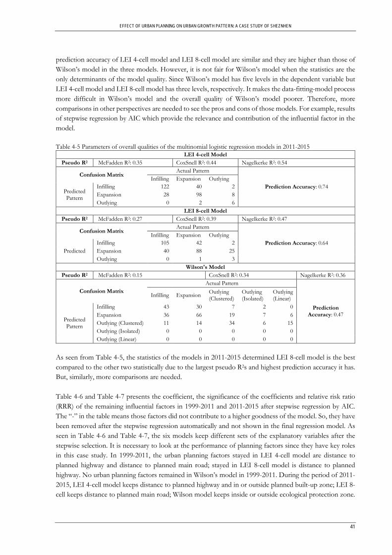
EFFECT OF URBAN PLANNING ON URBAN GROWTH PATTERN: A CASE STUDY OF SHEZNHEN
41
prediction accuracy of LEI 4-cell model and LEI 8-cell model are similar and they are higher than those of Wilson’s model in the three models. However, it is not fair for Wilson’s model when the statistics are the only determinants of the model quality. Since Wilson’s model has five levels in the dependent variable but LEI 4-cell model and LEI 8-cell model has three levels, respectively. It makes the data-fitting-model process more difficult in Wilson’s model and the overall quality of Wilson’s model poorer. Therefore, more comparisons in other perspectives are needed to see the pros and cons of those models. For example, results of stepwise regression by AIC which provide the relevance and contribution of the influential factor in the model. Table 4-5 Parameters of overall qualities of the multinomial logistic regression models in 2011-2015
LEI 4-cell Model Pseudo R2 McFadden R2: 0.35 CoxSnell R2: 0.44 Nagelkerke R2: 0.54
Confusion Matrix Actual Pattern
Prediction Accuracy: 0.74 Infilling Expansion Outlying
Predicted Pattern
Infilling 122 40 2 Expansion 28 98 8 Outlying 0 2 6
LEI 8-cell Model Pseudo R2 McFadden R2: 0.27 CoxSnell R2: 0.39 Nagelkerke R2: 0.47
Confusion Matrix Actual Pattern
Prediction Accuracy: 0.64 Infilling Expansion Outlying
Predicted Infilling 105 42 2 Expansion 40 88 25 Outlying 0 1 3
Wilson's Model Pseudo R2 McFadden R2: 0.15 CoxSnell R2: 0.34 Nagelkerke R2: 0.36
Confusion Matrix Actual Pattern
Prediction Accuracy: 0.47
Infilling Expansion Outlying (Clustered)
Outlying (Isolated)
Outlying (Linear)
Predicted Pattern
Infilling 43 30 7 2 0 Expansion 36 66 19 7 6 Outlying (Clustered) 11 14 34 6 15 Outlying (Isolated) 0 0 0 0 0 Outlying (Linear) 0 0 0 0 0
As seen from Table 4-5, the statistics of the models in 2011-2015 determined LEI 8-cell model is the best compared to the other two statistically due to the largest pseudo R2s and highest prediction accuracy it has. But, similarly, more comparisons are needed. Table 4-6 and Table 4-7 presents the coefficient, the significance of the coefficients and relative risk ratio (RRR) of the remaining influential factors in 1999-2011 and 2011-2015 after stepwise regression by AIC. The “-” in the table means those factors did not contribute to a higher goodness of the model. So, they have been removed after the stepwise regression automatically and not shown in the final regression model. As seen in Table 4-6 and Table 4-7, the six models keep different sets of the explanatory variables after the stepwise selection. It is necessary to look at the performance of planning factors since they have key roles in this case study. In 1999-2011, the urban planning factors stayed in LEI 4-cell model are distance to planned highway and distance to planned main road; stayed in LEI 8-cell model is distance to planned highway. No urban planning factors remained in Wilson’s model in 1999-2011. During the period of 2011-2015, LEI 4-cell model keeps distance to planned highway and in or outside planned built-up zone; LEI 8-cell keeps distance to planned main road; Wilson model keeps inside or outside ecological protection zone.

EFFECT OF URBAN PLANNING ON URBAN GROWTH PATTERN: A CASE STUDY OF SHEZNHEN
42
To sum up, LEI 4-cell model includes more planning factors in the regression analysis in total than LEI 8-cell model and Wilson’s model. Under this circumstance, LEI 4-cell model tells more information about the relative importance of planning factors since it compares more planning factors in the model. If we compare the significant coefficients of the remaining factors in LEI 4-cell model and LEI 8-cell model in 1999-2011 (see Table 4-6), those coefficients of same factors are similar in terms of scale and signs, except for population density. For example, distance to ocean is remaining in both LEI 4-cell model and LEI 8-cell model in 1999-2011, of which the coefficient in LEI 4-cell model is significant 3.6 and in LEI 8-cell is significant 3.9 when comparing the expansion pattern with infilling pattern, of which the coefficients in the two models are the same (1.4) when comparing the outlying pattern with infilling pattern. However, population density has very different significant coefficients in the two models in this period (2.8 in LEI 4-cell model relative to 1.8 in LEI 8-cell model when comparing the expansion pattern with infilling pattern, 5.1 in LEI 4-cell model relative to 1.8 in LEI 8-cell model when comparing the outlying pattern with infilling pattern). The reason can be found by looking back to the map of population density in 2000 (Figure 3-4) and the maps of urban growth patterns in 1999-2011 identified by LEI 4-cell method (Figure 4-4) and by LEI 8-cell method (Figure 4-5). The higher population density was present in the western Shenzhen where significantly more expansion pattern and outlying pattern were identified by LEI 4-cell method than by LEI 8-cell method. It makes the coefficients of the population density in LEI 4-cell model higher than those in LEI 8-cell mode. The differences between these two methods in terms of the relations with other factors are minor. When the comparison goes to 2011-2015 (see Table 4-7), only the percentage of existing urban within 1 km2 has significant coefficients in both models. Moreover, differences exist in the scales of the coefficients (-8.1 in LEI 4-cell model relative to -6.2 in LEI 8-cell model when comparing the expansion pattern with infilling pattern, -20 in LEI 4-cell model relative to -12.4 in LEI 8-cell model when comparing the outlying pattern with infilling pattern). Because there was a significantly larger percentage of outlying pattern and expansion pattern classified by LEI 4-cell than by LEI 8-cell in 2011-2015. Because the urban growth pattern classified by Wilson’s method is at pixel level rather than patch level and they are in five classes, it is unreasonable to compare the coefficients of Wilson’s model with the coefficients of LEI 4-cell model and LEI 8-cell model. Whereas, it is common in all the six models that the percentage of existing urban within 1 km2 has significantly larger absolute values of coefficients than other factors. The reason may be that all the three urban growth pattern classification methods are based on the density of the old urban areas surrounding the new grown urban, in which infilling pattern is encircled by the densest old urban areas. Thus, the higher the percentage of existing urban within 1 km2, the less likely to find expansion or outlying pattern than to find infilling pattern.

EFFECT OF URBAN PLANNING ON URBAN GROWTH PATTERN: A CASE STUDY OF SHEZNHEN
43
Table 4-6 Parameter estimates of the three multinomial logistic regression models in 1999-2011
Note: Baseline category is infilling pattern; s. means the coefficient is significant at the level of 0.05 (p-value < 0.05); n.s.=not significant at the level of 0.05 (p-value > 0.05); - means the factor is not shown in the model.
Category Coe. Sig. RRR Category Coe. Sig. RRR Category Coe. Sig. RRR Category Coe. Sig. RRRintercept 2.1 s. 8.1 2.0 s. 7.2 1.9 s. 6.4 -1.2 n.s. 0.3distance to city center - - - - - - - - - - - -distance to lake 1.4 s. 4.2 - - - 0.4 n.s. 1.5 0.7 n.s. 2.1distance to ocean 3.6 s. 37.1 3.9 s. 48.4 - - - - - -distance to port -3.9 s. 0.0 -3.2 s. 0.0 - - - - - -elevation - - - - - - - - - - - -slope - - - -1.1 n.s. 0.3 - - - - - -% of existing urbanwithin 1 km2
-7.0 s. 0.0 -6.9 s. 0.0 -3.2 s. 0.0 -1.8 n.s. 0.2
distance to existingmain road
2.9 s. 18.7 2.4 s. 10.8 -1.9 n.s. 0.1 3.3 s. 28.2
distance to existinghighway
- - - - - - - - - - - -
GDP per capita - - - - - - 0.2 n.s. 1.2 -6.0 n.s. 0.0population density 2.8 s. 17.2 1.8 s. 6.1 - - - - - -inside or outsideSEZ
- - - - - - - - -
distance to plannedhighway
0.8 n.s. 2.3 1.2 s. 3.3 - - - - - -
distance to plannedmain road
-1.8 s. 0.2 - - - - - - - - -
inside or outsideplanned ecologicalprotection zone
- - - - - - - - - - - -
inside or outsideplanned built up zone
- - - - - - - - - - - -
intercept 1.7 s. 5.7 -0.1 n.s. 0.9 4.0 s. 53.4 1.4 s. 4.2distance to city center - - - - - - - - - - - -distance to lake 2.0 n.s. 7.3 - - - 0.7 n.s. 2.0 -3.3 n.s. 0.0distance to ocean 1.4 n.s. 4.2 1.4 n.s. 4.2 - - - - - -distance to port -1.9 n.s. 0.1 1.1 n.s. 3.0 - - - - - -elevation - - - - - - - - - - - -slope - - - 2.4 n.s. 10.8 - - - - - -% of existing urbanwithin 1 km2
-16.1 s. 0.0 -17.0 s. 0.0 -7.5 s. 0.0 -10.7 s. 0.0
distance to existingmain road
1.4 n.s. 4.1 2.4 n.s. 0.5 -5.0 s. 0.0 1.8 n.s. 5.9
distance to existinghighway
- - - - - - - - - - - -
GDP per capita - - - - - - -0.5 n.s. 0.6 1.4 n.s. 4.1population density 5.1 s. 172.1 1.8 s. 100.7 - - - - - -inside or outsideSEZ
- - - - - - - - - - - -
distance to plannedhighway
-0.7 n.s. 0.5 1.2 n.s. 0.3 - - - - - -
distance to plannedmain road
-2.2 n.s. 0.1 - - - - - - - - -
inside or outsideplanned ecologicalprotection zone
- - - - - - - - - - - -
inside or outsideplanned built up zone
- - - - - - - - - - - -
Expansion
Outlying(Clustered)
Outlying(Isolated)
Outlying(Linear)
Expansion
Outlying
LEI 4-cell LEI 8-cell
Expansion
Outlying
FactorWilson Wilson

EFFECT OF URBAN PLANNING ON URBAN GROWTH PATTERN: A CASE STUDY OF SHEZNHEN
44
Table 4-7 Parameter estimates of the three multinomial logistic regression models in 2011-2015
Note: Baseline category is infilling pattern; s. means the coefficient is significant at the level of 0.05 (p-value < 0.05); n.s.=not significant at the level of 0.05 (p-value > 0.05); - means the factor is not shown in the model.
4.3.3. Spatial Autocorrelation Test From Table 4-8, we can learn that the residuals of every outcome category of the six regression models are not significantly autocorrelated. Because the values of Moran’s I are very close to zero, which indicates perfect randomness, and the diagnosis produced by Moran’s I test function in R indicates the residuals are
Category Coe. Sig. RRR Category Coe. Sig. RRR Category Coe. Sig. RRR Category Coe. Sig. RRRintercept 5.5 s. 248.4 3.7 s. 40.5 1.6 s. 5.2 1.3 n.s. 3.8distance to city center -4.4 s. 0.0 - - - - - - - - -distance to lake - - - - - - - - - - - -distance to ocean -2.3 s. 0.1 -0.9 n.s 0.4 - - - - - -distance to port 5.3 s. 193.4 - - - - - - - - -elevation - - - - - - - - - - - -slope -3.3 s. 0.0 - - - 0.9 n.s. 2.5 -15.7 n.s. 0.0% of existing urbanwithin 1 km2
-8.1 s. 0.0 -6.2 s. 0.0 -2.8 s. 0.1 -4.7 s. 0.0
distance to existingmain road
-3.9 s. 0.0 - - - - - - - - -
distance to existinghighway
- - - - - - - - - - - -
GDP per capita - - - - - - - - - - - -population density -2.8 s. 0.0 - - - - - - - - -inside or outsideSEZ
- - - -1.1 s. 0.3 - - - - - -
distance to plannedhighway
-2.8 n.s. 0.0 - - - - - - - - -
distance to plannedmain road
- - - -1.7 s. 0.2 - - - - - -
inside or outsideplanned ecologicalprotection zone
- - - - - - -0.5 n.s. 0.6 -8.2 n.s. 0.0
inside or outsideplanned built up zone
-0.3 n.s. 1.3 - - - - - - - - -
intercept 4.7 n.s. 112.6 3.0 s. 20.8 3.4 s. 30.3 1.6 s. 5.1distance to city center 1.8 n.s. 5.9 - - - - - - - - -distance to lake - - - - - - - - - - - -distance to ocean -2.6 n.s. 0.1 -2.8 s. 0.1 - - - - - -distance to port -0.8 n.s. 0.4 - - - - - - - - -elevation - - - - - - - - - - - -slope -3.5 n.s. 0.0 - - - -1.1 n.s. 0.3 -2.3 n.s. 0.1% of existing urbanwithin 1 km2
-20.0 s. 0.0 -12.4 s. 0.0 -8.2 s. 0.0 -8.0 s. 0.0
distance to existingmain road
-5.7 n.s. 0.0 - - - - - - - - -
distance to existinghighway
- - - - - - - - - - - -
GDP per capita - - - - - - - - - - - -population density 2.9 n.s. 18.3 - - - - - - - - -inside or outsideSEZ
-0.4 n.s. 0.7 - - - - - -
distance to plannedhighway
0.5 n.s. 1.7 - - - - - - - - -
distance to plannedmain road
- - - -0.9 n.s 2.6 - - - - - -
inside or outsideplanned ecologicalprotection zone
- - - - - - -1.0 n.s. 0.4 0.7 n.s. 2.1
inside or outsideplanned built up zone
-2.2 s. 0.1 - - - - - - - - -
Outlying
Expansion ExpansionOutlying(Isolated)
Factor
Expansion
LEI 4-cell LEI 8-cell Wilson Wilson
Outlying(Clustered)
Outlying(Linear)
Outlying

EFFECT OF URBAN PLANNING ON URBAN GROWTH PATTERN: A CASE STUDY OF SHEZNHEN
45
under randomisation. As a result, the parameter estimates of the six models are not influenced by the spatial autocorrelations. Table 4-8 Results of spatial autocorrelation test on model residuals by calculating Moran’s I
Outcome Residuals Lei 4-cell Lei 8-cell Wilson's
Moran's I Diagnosis Moran's I Diagnosis Moran's I Diagnosis 1999-2011
Infilling 0.01 random 0.00 random -0.04 random Expansion -0.01 random -0.01 random -0.04 random Outlying -0.08 random -0.05 random - - Outlying (Clustered) - - - - -0.05 random Outlying (Isolated) - - - - 0.01 random Outlying (Linear) - - - - 0.00 random
Outcome Residuals 2011-2015 Infilling -0.03 random -0.02 random -0.01 random Expansion -0.03 random -0.01 random -0.03 random Outlying -0.01 random -0.03 random - - Outlying (Clustered) - - - - 0.02 random Outlying (Isolated) - - - - -0.02 random Outlying (Linear) - - - - 0.01 random
The summaries can be made like the following: In 1999-2011, LEI 4-cell model has similar overall quality as LEI 8-cell model. In 2011-2015, LEI 4-
cell model has higher overall quality than LEI 8-cell model in 2011-2015. In addition, their absolute value of R2 and prediction accuracy are sufficient to be “good” models. Although Wilson’s model provides information about the detailed outlying patterns, the degree of sample dataset fitting model is too low (R2 and prediction accuracy are low) to be a “good” model.
Wilson’s model has five urban growth patterns, which are in pixel level, in the dependent variable. Hence, the statistics indicating overall model quality and parameter estimates of these three models in each period are not comparable. However, Wilson’s method produced problems during distinguishing some of the clustered and linear patterns, see the example in Figure 4-7. It will cause incorrect parameter estimates for each influential factor. Therefore, Wilson’s model cannot be the one to be closely analysed to give implications on the relationships between influential factors and urban growth patterns.
LEI 4-model compares more urban planning factors than LEI 8-cell model or Wilson’s model in both periods.
The contradictions between the significant coefficients of LEI 4-cell model and LEI 8-cell model in both periods are reasonable.
The parameters estimated in the six models are not biased by the spatial autocorrelations. Due to the reasons listed above, I picked LEI 4-cell models in the two periods to look closely.
4.4. Relationships between Urban Growth Pattern and Its Determinants This section demonstrates the relationships between urban growth patterns and their influential factors in 1999-2011 and 2011-2015 by interpreting the outputs of LEI 4-cell models in these two periods. It is necessary to be reminded that the linear variables of the model were normalised to 0-1 before they were

EFFECT OF URBAN PLANNING ON URBAN GROWTH PATTERN: A CASE STUDY OF SHEZNHEN
46
fitted by the model. In this way, we can know the relative importance of each influential factor by simply comparing the absolute value of their coefficients.
4.4.1. Relationships between Urban Growth Pattern and Urban Planning Factors In this section, only the relationships between urban growth patterns and urban planning factors are presented, the next section 4.4.2 shows the interpretation of other influential factors. Table 4-6 presents the result parameters obtained from LEI 4-cell model in 1999-2011. As seen in the table, during the period of 1999-2011, distance to planned highway and distance to planned main road were important planning factors in forming expansion or outlying pattern relative to being infilling pattern. However, they have relatively small obsolute values of coefficients compared to the rest of remained predictors. In the case of being expansion pattern relative to being infilling pattern, distance to planned highway and distance to planned main road obtained coefficients of 0.8 and -1.8, respectively. However, only the coefficient of distance to planned main road (-1.8) is significant. Hence, only distance to planned main road can help us differentiate the expansion pattern and infilling pattern in 1999-2011. The RRR of distance to planned main road is below 1. Thus, it is more likely for an urban growth patch to be expansion relative to being infilling if the distance to planned main road in 1999-2011 decreased. In the case of being outlying pattern relative to infilling pattern, the coefficients of distance to planned highway and distance to planned main road are -0.7 and -2.2, respectively, but both of them are not significant. Therefore, neither distance to planned highway nor distance can differentiate the outlying pattern from infilling pattern in 1999-2011. The obtained parameters from running LEI-4 model based on the data of 2011-2015 are shown in Table 4-7. During 2011-2015, only distance to planned highway and distance to planned built-up zone stayed in the model. In the case of being expansion relative to infilling pattern, both of the coefficients of distance to planned highway and inside or outside planned built-up zone are not significant. As a result, these two urban planning factors do not contribute to the differentiation of the expansion pattern and infilling pattern in 2011-2015. In the case of being outlying relative to infilling pattern, the coefficient of distance to planned highway is not significant while inside or outside planned built-up zone has a significant coefficient of -2.2. However, the absolute value of the coefficient is less than most of the other influential factors. The RRR indicates that the relative risk of being an outlying pattern than infilling pattern increases if the urban growth patch was outside the planned built-up zone rather than inside the planned built-up zone. In short, the outlying pattern is more likely to happen outside the planned built-up zone while the infilling pattern is more likely to occur inside the planned built-up zone. To sum up, distance to planned main road in 1999-2011 and inside or outside planned built-up zone in 2011-2015 in the models provided meaningful indications on the effects of planned main roads in 1999-2011 and planned built-up zone in 2011-2015 upon urban growth patterns. Furthermore, they provided similar results as assumed. To begin the analysis of the reasons behind the different performances of the built-up plan in 1999-2011 and 2011-2015, the planned built-up zones in the two periods were simply checked by overlaying the plan maps on the maps urban growth pattern identified by LEI 4-cell method (see Annex I). In 1999-2011, a large proportion of urban growth was out of the planned built-up zone, especially in the non-SEZ region, and it was a mixture of infilling, expansion and outlying patterns. Thus, it confused the regression model on the significance of inside or outside built-up zone. Deng et al. (2018) believed that the dual land management system in SEZ and non-SEZ did not coordinate with the needs of rapid urban development of Shenzhen, it resulted in the chaotic urban construction throughout the non-

EFFECT OF URBAN PLANNING ON URBAN GROWTH PATTERN: A CASE STUDY OF SHEZNHEN
47
SEZ zone. So, the assumption that the government encouraged the increase of the density of urban areas through plans fell behind the demand for large and fast urban development from people in this period. Despite that the estimated urban land demand was below the actual land demand for city developing, the uncertainty factors, such as big city events, can also weaken the legal validity and guidance of the construction plans (Yang & Wang, 2008). In addition, the mixture of the three patterns outside planned built-up zone was also inside the planned ecological protection zone. For these reasons, the studied land use plans are not important for setting apart the expansion pattern or outlying pattern from infilling pattern in 1999-2011. In 2011-2015, very less outlying pattern but almost all of the infilling pattern occurred inside the planned built-up zone. It may be the results of the intensification method the government took for the effective uses of the limited land resource for built-up in this period. Hence, inside or outside the planned built-up zone has a significant effect on the outlying pattern and infilling pattern from the model. Regarding the performances of distance to planned main road and distance to planned highway, it is hard to tell the reasons by only looking at the distance maps of planned roads and urban growth pattern maps. But we can assume that whether the government implemented the transportation plans (planned main road and planned highway) in the plan period or not highly influence people’s choice of the locations of urban construction. It might partially explain the performances. For example, when people only cared about the already implemented main road, the coefficient of distance to planned main road is not significant if most of the planned main roads were not implemented. In order to test the assumption, the implementation statuses (i.e. implemented or not implemented by the end of plan period) of the those planned roads were checked in the historical satellite images in Google Earth Pro. Then, maps of distance to the actually implemented main road in the 1999-2011 and 2011-2015 can be found in Annex II. Next, distance to implemented highway and distance to implemented main road replaced distance to planned highway and distance to planned main road in LEI 4-cell models in the two periods. Following the steps of outlier elimination, multicollinearity test, running model and spatial autocorrelation test as the six models did before, the model parameters in 1999-2011 and 2011-2015 are shown in Annexure III. The prediction accuracies and pseudo R2s of the regression models did not change much. The modelling results show that distance to implemented highway can differentiate expansion pattern from infilling pattern in 1999-2011 while distance to planned highway cannot. However, neither distance to implemented highway nor distance to planned highway cannot explain the difference between outlying and infilling in 1999-2011. It can be concluded that the implemented highway in the plans is a more important factor for expansion than merely the planned highways on the plan map in this time phase. The closer to the implemented highway, the more likely for infilling pattern to happen. It is totally different from the assumption that people more likely to extend the existing urban towards the planned highways. Referring back to the urban growth pattern map in 1999-2011 (Figure 4-4) and maps of distance to implemented highway in 1996-2010 (Annex II), a high proportion of infilling pattern was close to the implemented highways. In contrast, the implementation status of planned main roads was not important in 1999-2011 since the distance to planned main road has a significant coefficient but the distance to implemented main road does not. In 2011-2015, distance to implemented highway does show up in the new regression model in 2011-2015. It means that the implementation status of the planned highway in 2011-2015 does not make any differences in differentiating the expansion or outlying from infilling. Distance to implemented main road stayed in the new LEI 4-cell model in 2011-2015 while distance to planned main road did not. Moreover, if distance to implemented main road increases, it is more likely to find infilling than expansion. Unfortunately, it is not easy to explain the reason for why distance to implemented highway in 1999-2011 and distance to implemented main road in 2011-2015 can set apart different patterns. Because the

EFFECT OF URBAN PLANNING ON URBAN GROWTH PATTERN: A CASE STUDY OF SHEZNHEN
48
implementation statuses were determined by comparing the planned roads with satellite images of 2010 or 2015. No further information about when those roads constructed. If the roads had been built up before the urban growth patterns happen at the same places, we can infer that the actually implemented roads from transportation plan facilitate people to create the corresponding urban growth patterns as the models say. The reflection on the effects of urban plans on urban growth patterns are as following: The land use plans in 1996-2010, i.e. planned built-up zone, planned ecological protection zone, did
not influence the coalescence or diffusion of the urban Shenzhen since the land use plan factors, inside or outside the built-up zone and inside or outside the ecological zone, were not significantly correlated with any of the patterns in this period. In addition, these land use plans were not efficiently implemented since the built-ups have exceeded the planned built-up zones and encroached the officially protected ecological resources. The planned main roads in the Master Plan of Shenzhen 1996-2010 facilitated the expansion growth towards them instead of infilling growth, and it made the city sprawled and the existing urban clusters, e.g. different towns, connected. Then, a higher integration of people from different parts of the city could be achieved.
The planned built-up zone in the Master Plan of Shenzhen 2010-2020 worked well in letting the infilling pattern inside the built-up zone rather than the outlying pattern. It increased the degree of densification of the urban. However, the planned main road and planned highway in 2011-2015 did not significantly affect urban growth patterns.
Master Plan of Shenzhen 1996-2010 and Master Plan of Shenzhen 2010-2020 have slightly affected the urban growth patterns in Shenzhen as suggested by the absolute values of the coefficients of the urban planning factors (i.e. distance to planned highway, distance to main road, inside or outside the planned built-up zone and inside or outside the ecological protection zone). Because the implementation of these master plans has been weakened by market mechanism and other thematic plans. According to Tian & Shen (2011), part of the land is not compulsory to be developed as planned in the master plan after required legal procedures, if the market provided more benefits than plan. The plans compiled for different themes for different time phase also contradicted with master plans to some extent, for example, Land Use Plan of Shenzhen 2006-2020 designated different amount of urban area (976 km2) in 2020 with Master Plan of Shenzhen 2010-2020 (890 km2). It led to the poor implementation of the land use plan in the master plan for Shenzhen as well.
4.4.2. Relationships between Urban Growth Pattern and Socio-economic, Physical, Accessibility, Proximity and Neighbourhood Influential Factors
The relationships between urban growth patterns and other influential factors (socio-economic factors, physical factors, accessibility factors, proximity factors and neighbourhood factor) in 1999-2011 are indicated by the parameters of LEI 4-cell model in Table 4-6. As illustrated before, the percentage of existing urban area within 1 km2 contributes the largest to the outcome of being expansion pattern or outlying relative to infilling pattern in both 1999-2011 and 2011-2015. Moreover, it is more possible for a new urban patch to be expansion relative or outlying to being infilling when less old urban is in its neighbourhood. Regarding other factors, the lower the distance to lake, distance to ocean, distance to existing main road or higher the population density, the more likely to find infilling pattern than expansion in 1999-2011. From the dataset, there were many existing urban patches around either the lakes, ocean, existing main road or in the district with high population density. In the light of this, the new grown urban patches near or in these places are of great possibility to be recognised as infilling pattern by the LEI 4-cell method. In other words, the closer to the lakes, ocean or main road or in a more populated district in 1999, the higher the compactness of urban patches in 2011. Similarly, a population density increase would lead to an increase of

EFFECT OF URBAN PLANNING ON URBAN GROWTH PATTERN: A CASE STUDY OF SHEZNHEN
49
possibility of being outlying relative to infilling in 1999-2011. However, distance to lake, distance to ocean, distance to port and distance to existing main road obtained non-significant coefficients in this model. The relationships between urban growth patterns and other influential factors in 2011-2015 are indicated by the parameters of LEI 4-cell model in Table 4-7. Contrary to results obtained in the model of 1999-2011, distance to city centre, distance to ocean, slope, distance to existing main road and population density are significantly and negatively correlated with the probability of being expansion than infilling. There are two possible reasons: 1) By 2011, urban development, which was close to either city centre, ocean or existing main road or in flat or low populated places, has been in high density after long-time fast urbanisation. Because, those places are highly attracted to urban developments (Liu et al., 2010). It is difficult for many infilling patches to happen in those areas, but it is easier for the new urban to grow in the edge of those places in 2011; 2) the random samples with minimal interval of 200m biases the results if they included more expansion than infilling around the city centre, ocean or existing main road and so on. In the case of being outlying pattern relative to being infilling pattern, no predictors have significant coefficients except the proportion of old urban within 1 km2. It is supersizing that the SEZ did not affect the urban growth pattern too much in both periods from the model results. This might because the city was growing beyond the SEZ due to the increasing urban development demand of people in the commercial, access to the neighbouring city and other fields (Deng et al., 2018). From the results, the urban plans together with the socio-economic factors, physical factors, proximity factors, accessibility factors and neighbourhood factors resulted in the urban landscape of Shenzhen. It assists the inference made by Li et al. (2005) that the spatial pattern of the landscape of Shenzhen could be explained by the changes in population density, economic growth, transport network and the role of local government.
4.5. Reflection on the Data, Methodology of the Case Study This section mainly provides the reflection on the datasets and the methodology I used in this case study since the reflection on the study results have already been made in the other sections in the chapter. The reflection on the datasets is as follows: The land cover dataset is the biggest limitation of this case study. As mentioned in section 3.2.1, the
areas of original urban land cover fluctuated over time. But other researchers believed that the urban area of Shenzhen was increasing consistently through classifying urban land on remote sensing imagery (Lv et al., 2009). Then, the correction method on land cover data has been applied, based on the assumption that urbanization was irreversible in Shenzhen, to make use of this secondary data. However, this assumption does not completely fit with the case of Shenzhen. During the exploration of the urban growth in Shenzhen, I found that there were few urban areas changed to non-urban areas in Shenzhen. From the example in Annex IV, the buildings existing in 2011 have been demolished, and the land became bare land in 2013, then, the land was about half built-up in 2015. Following the assumption, this change would be covered since this land stayed urbanised after 2011. In addition, the infilling pattern will be identified if we only look at the urban growth pattern during 2013-2015. But it does not matter too much in this study since such phenomena are very few. Moreover, the land cover data correction made the urban growth in this study larger than in reality since the errors of the land cover classification have been cumulated in the correction process. As the example in Annex V shown, the farmland in 2013 has been wrongly classified as urban land in the original land cover dataset, then it was treated as urban land as well in the corrected land cover dataset although the classifications in
EFFECT OF URBAN PLANNING ON URBAN GROWTH PATTERN: A CASE STUDY OF SHEZNHEN
50
other years (e.g. 2011and 2015) were right. In light of this, the area of urban growth increases after data correction.
Regarding the data of urban plans, the accuracy was limited by the accuracy of the plan maps and the errors of digitization of the plan maps. The available maps of Master Plan of Shenzhen 1996-2010 were completed at the end of 1996, they are too old to offer very high-accuracy spatial information about the plans. When I was exploring the urban plan maps, some of the existing roads before 1996 in the plan map were shifted from their places in reality. But the shifting scale was acceptable (about 10m-40m). Therefore, we can assume that other items in the plan map, such as planned roads, built-up zone, in the plan maps probably were shifted as well. The digitization errors, such as missing digitization of the points in very complex polygons, also decrease the overall accuracy of the data of planning factors, e.g. inside or outside the built-up zone.
The distance maps of the influential factors were produced by running the Euclidean Distance tool in ArcMap, however, it would be better to calculate the distance based on the road network if the data is available. Because people are approaching the points of interest, e.g. city centre, the trough road network in reality. Therefore, the distance by road network to the city centre is more realistic than the Euclidean distance to the city centre.
The reflection on the methodology is as follows: Except searching the potential factors influencing urban growth pattern in the literature, the advice
from planning or geography expert in Shenzhen should also be considered as an essential source. Without abundant background knowledge of Shenzhen, some important factors may be ignored.
Wilson’s method classifies the urban growth into five separate patterns which contain most of the patterns happened in reality in details, but it is more suitable to the case with low urban growth speed other than Shenzhen. In Shenzhen’s case, the urban grew at an impressive speed due to the special role it plays in the economic development of China. Even an urban growth within a three-year period is large, for example, the new urban in 1999-2001 was around 48 km2. Pixel-based approach (Wilson’s method in this study) in Shenzhen can lead to the extremely high proportion of outlying pattern but a low proportion of infilling pattern and expansion pattern. For this reason, it is difficult to figure out the spatial characteristics of the infilling pattern and expansion pattern in such a big city since they were very few and dispersed everywhere. The error in land cover dataset impacted the identified urban growth patterns by Wilson’s method as well. According to the model developer, Wilson et al. (2003), even a slight error of land cover classification could lead to the wrong detection of urban growth pattern. Although the land cover data correction has been applied, the accuracy of the land cover data used for urban growth pattern identification cannot be fully trusted. Therefore, the classification of urban growth pattern by Wilson’s method was disturbed by the dataset quality. Similarly, the identification by LEI 4-cell or LEI 8-cell was disturbed but it is less vulnerable than that by Wilson’s method.
The time interval for analysing and the criteria for separating urban growth patterns based on the computed LEI are of great importance since it highly influences the amount of each urban growth pattern we will obtain. As discussed in section 4.2, Lv et al. (2009), who computed a similar index as LEI but adopted a shorter interval and applied different criteria to differentiate infilling, expansion and outlying patterns, acquired different dominated pattern in Shenzhen during 1988-1999. This gives us an implication that we should be critical to select the time periods and rules to identify urban growth patterns when analysing the urban growth patterns. The time periods should be fitted into the case study to make benefits for the research. But the criteria of differentiating patterns do not matter significantly since the results can be interpreted and analysed based on the criteria. In this case study, I

EFFECT OF URBAN PLANNING ON URBAN GROWTH PATTERN: A CASE STUDY OF SHEZNHEN
51
am analysing the urban growth patterns during the master plan phase and linking to the urban plans. Therefore, the time periods I chose fits the purpose of this case study.
With regards to the neighbouring rules for defining a patch, the 4-cell neighbourhood rule is more suitable in this case than 8-cell neighbourhood rule. In Shenzhen’s case, the urban growth rate was remarkable, thus, 8-cell neighbourhood rule is more like to form a large patch which contains a larger range of geographical information, e.g. a larger range of slope. However, such a large patch only can be assigned to one single urban growth pattern. It can confuse the regression model that which value of the slope is really fitting this pattern?
Multinomial regression model was capable to distinguish different urban growth patterns based on the geographical information and it provided reasonable results. It also offers the indication of the degree of the influence made by these influential factors on urban growth patterns. This case study only explored the effects of those selected factors on the urban growth patterns. For more information about how the non-developed area changes to any of these patterns, one more category, i.e. non-urban, should be added to the dependent variable.


EFFECT OF URBAN PLANNING ON URBAN GROWTH PATTERN: A CASE STUDY OF SHEZNHEN
53
CONCLUSIONS
The objective of this study was to understand the relationship between urban master plans and urban growth patterns in Shenzhen. Few studies have been conducted to detect the urban growth patterns in Shenzhen and analyse the reason behind these patterns, but the analysis of the effects of urban planning was missed in those studies. Three main steps were involved in this thesis: identifying the historical urban growth patterns from land cover maps; identifying the potential influential factors of urban growth pattern in Shenzhen including urban plans as well as socio-economic, physical, proximity, neighbourhood and accessibility factors. To understand what happened in the long history of Shenzhen in the three master plan periods, which are 1986-2000, 1996-2010 and 2010-2020, the urban growth patterns in 1988-1999, 1999-2011 and 2011-2015 were detected due to the data limitation. In the process of identifying the urban growth patterns, three separate methods were used because of their pros and cons. They are the method developed by Wilson et al. (2003), Landscape Expansion Index following 4-cell neighbourhood rule (LEI 4-cell) and Landscape Expansion Index following 8-cell neighbourhood rule (LEI 8-cell). They provided different information in terms of the compositions of urban growth patterns. Wilson’s method detected a higher percentage of outlying pattern in all of the three periods while LEI 4-cell and LEI 8-cell detected a higher percentage of expansion in 1988-1999 and 1999-2011 but a higher percentage of infilling in 2011-2015. By reviewing the master plan documents and literature, the plans which might have influences on the urban development were selected. In addition, potential factors have driven or have differentiated the urban growth were extracted from the studies in Shenzhen. Through digitizing the plan maps, collecting secondary data, the dataset used for multinomial logistic regression modelling was prepared. Following the steps for correcting the noisy data and enhancing the reliability of the multinomial logistic regression models, the six models came out. The parameters of them represent the reaction of each influential factors on urban growth pattern by three identification methods in two plan periods. After comparing the model output, the LEI 4-cell model was selected to be analysed closely since it has prediction accuracies of 71% in 1999-2011 and of 74% in 2011-2015. Also, LEI 4-cell model compares more urban planning factors in total than LEI 8-cell model and Wilson’s model. Compared to that, the regression models for the urban growth patterns identified by the LEI 8-cell method have less explained variance. The drawback of Wilson’s method is distinguishing some linear urban growth from clustered urban growth in this case study. By interpreting and discussing the LEI 4-cell model results, the master plans together with other socio-economic, physical, proximity, accessibility and neighbourhood factors shaped the urban of Shenzhen. The planned main road in Master Plan of Shenzhen 1996-2010 and the planned built-up zone in the Master Plan of Shenzhen 2010-2020 affected the urban growth pattern in 1999-2011 and 2011-2015, but they contributed less than most of the other factors, e.g. distance to ocean. In addition, the actually implemented highways in 1999-2011 and the implemented main roads in 2011-2015 also had effects on the urban growth patterns. City centre, lakes, ocean, ports, slope, density of neighbourhood old urban, old main roads and population density had different degrees of influence on the evolution of urban growth patterns in Shenzhen.

EFFECT OF URBAN PLANNING ON URBAN GROWTH PATTERN: A CASE STUDY OF SHEZNHEN
54
The corrected land cover dataset and data of the factors influencing urban growth patterns are crucial in this case study, accurately classified land cover data of Shenzhen would provide more realistic results about the master plans’ effects on urban growth patterns. The patch-based urban growth pattern classification method (LEI) and the pixel-based urban growth pattern identification method (Wilson’s method) have their own benefits when detecting the growth patterns. LEI presented clearer composition and configuration of urban growth patterns on the map and the patterns identified by LEI satisfied regression model. Wilson’s method provided more detailed urban growth patterns. Multinomial regression model helped to identify the effects of the urban plans on the infilling, expansion and outlying patterns. The further studies can be set on the exploration of more urban growth patterns, not only on a horizontal level but also on a vertical level. For the big city like Shenzhen, the urban was not only extending from the old urban to the agricultural land but increasing the building height as well. The increase or decrease of the building height can also be part of the criteria to define the urban growth patterns. In addition, the dependent variable in this study can be extended to non-urban, infilling, expansion and outlying to figure out how these patterns changed from non-urban land and what roles did the master plans in this process. This case study offers a way to investigate the importance of urban planning and how it influences the urban growth patterns and also gives implication to the urban planners and policy-makers in Shenzhen to develop valuable plans for Master Plan of Shenzhen 2020-2030. If the urban plans have similar effects on the urban growth patterns in the coming plan period as the study explored for the past, urban planners should watch out the new urban development outside the built-up zone since it is outlying and disconnected with the existing urban. If it is applicable, further researches can focus on the attribute of the outlying growth. If most of the outlying growth areas are informal settlements, the monitoring and management of the land beyond the built-up zone should be improved. Moreover, the planning of the new main roads can also be the tool to guide the expansion of the old urban towards the place where the planned roads would be located.

EFFECT OF URBAN PLANNING ON URBAN GROWTH PATTERN: A CASE STUDY OF SHEZNHEN
55
LIST OF REFERENCES Aguilera, F., Valenzuela, L. M., & Botequilha-Leitão, A. (2011). Landscape metrics in the analysis of urban
land use patterns: A case study in a Spanish metropolitan area. Landscape and Urban Planning, 99(3–4), 226–238. https://doi.org/10.1016/J.LANDURBPLAN.2010.10.004
Aithal, B. H., & Ramachandra, T. V. (2016). Visualization of urban growth pattern in Chennai using geoinformatics and spatial metrics. Journal of the Indian Society of Remote Sensing, 44(4), 617–633. https://doi.org/10.1007/s12524-015-0482-0
Bai, X., Shi, P., & Liu, Y. (2014). Society: Realizing China’s urban dream. Nature, 509(7499), 158–160. https://doi.org/10.1038/509158a
Bhatta, B. (2010). Analysis of urban growth and sprawl from remote sensing data. Berlin, Germany: Springer-Verlag Berlin Heidelberg. https://doi.org/10.1007/978-3-642-05299-6
Braimoh, A. K., & Onishi, T. (2007). Spatial determinants of urban land use change in Lagos, Nigeria. Land Use Policy, 24(2), 502–515. https://doi.org/10.1016/J.LANDUSEPOL.2006.09.001
Camagni, R., Gibelli, M. C., & Rigamonti, P. (2002). Urban mobility and urban form: the social and environmental costs of different patterns of urban expansion. Ecological Economics, 40(2), 199–216. https://doi.org/10.1016/S0921-8009(01)00254-3
Chen, J., Chang, K., Karacsonyi, D., & Zhang, X. (2014). Comparing urban land expansion and its driving factors in Shenzhen and Dongguan, China. Habitat International, 43, 61–71. https://doi.org/10.1016/J.HABITATINT.2014.01.004
Chen, Y., Li, X., Liu, X., Ai, B., & Li, S. (2016). Capturing the varying effects of driving forces over time for the simulation of urban growth by using survival analysis and cellular automata. Landscape and Urban Planning, 152, 59–71. https://doi.org/10.1016/j.landurbplan.2016.03.011
Cheng, J., & Masser, I. (2003). Urban growth pattern modeling: a case study of Wuhan city, PR China. Landscape and Urban Planning, 62(4), 199–217. https://doi.org/10.1016/S0169-2046(02)00150-0
Deng, Y., Fu, B., & Sun, C. (2018). Effects of urban planning in guiding urban growth: Evidence from Shenzhen, China. Cities, 83, 118–128. https://doi.org/10.1016/j.cities.2018.06.014
Dou, P., & Chen, Y. (2017). Dynamic monitoring of land-use/land-cover change and urban expansion in Shenzhen using Landsat imagery from 1988 to 2015. International Journal of Remote Sensing, 38(19), 5388–5407. https://doi.org/10.1080/01431161.2017.1339926
Field, A. (2013). Discovering statistics using IBM SPSS statistics (4th ed.). London, England: SAGE Publications Ltd.
Hall, P., & Tewder-Jones, M. (2011). Planning, planners and plans. In Urban and Regional Planning (5th ed., pp. 1–10). London, England: Routledge.
Hepinstall-Cymerman, J., Coe, S., & Hutyra, L. R. (2013). Urban growth patterns and growth management boundaries in the Central Puget Sound, Washington, 1986-2007. Urban Ecosystems, 16(1), 109–129. https://doi.org/10.1007/s11252-011-0206-3
Herold, M., Couclelis, H., & Clarke, K. C. (2005). The role of spatial metrics in the analysis and modeling of urban land use change. Computers, Environment and Urban Systems, 29(4), 369–399. https://doi.org/10.1016/J.COMPENVURBSYS.2003.12.001
Huang, L., & Xie, Y. (2012). The plan-led urban form: a case study of Shenzhen. In 48th ISOCARP Congress 2012 (pp. 1–10). Perm,Russia.
Huang, X., Xia, J., Xiao, R., & He, T. (2017). Urban expansion patterns of 291 Chinese cities, 1990–2015. International Journal of Digital Earth, 62–77. https://doi.org/10.1080/17538947.2017.1395090

EFFECT OF URBAN PLANNING ON URBAN GROWTH PATTERN: A CASE STUDY OF SHEZNHEN
56
Kam Ng, M., & Tang, W.-S. (2004). The role of planning in the development of Shenzhen, China: Rhetoric and realities. Eurasian Geography and Economics, 45(3), 190–211. https://doi.org/10.2747/1538-7216.45.3.190
Kühn, I., & Dormann, C. F. (2012). Less than eight (and a half) misconceptions of spatial analysis. Journal of Biogeography, 39(5), 995–998. https://doi.org/10.1111/j.1365-2699.2012.02707.x
Li, G., Sun, S., & Fang, C. (2018). The varying driving forces of urban expansion in China: Insights from a spatial-temporal analysis. Landscape and Urban Planning, 174, 63–77. https://doi.org/10.1016/j.landurbplan.2018.03.004
Li, W., Wang, Y., Peng, J., & Li, G. (2005). Landscape spatial changes associated with rapid urbanization in Shenzhen, China. International Journal of Sustainable Development & World Ecology, 12(3), 314–325. https://doi.org/10.1080/13504500509469641
Liu, J., Zhang, Z., Xu, X., Kuang, W., Zhou, W., Zhang, S., … Jiang, N. (2010). Spatial patterns and driving forces of land use change in China during the early 21st century. Journal of Geographical Sciences, 20(4), 483–494. https://doi.org/10.1007/s11442-010-0483-4
Liu, X., Li, X., Chen, Y., Tan, Z., Li, S., & Ai, B. (2010). A new landscape index for quantifying urban expansion using multi-temporal remotely sensed data. Landscape Ecology, 25(5), 671–682. https://doi.org/10.1007/s10980-010-9454-5
Liu, Y., He, Q., Tan, R., Liu, Y., & Yin, C. (2016). Modeling different urban growth patterns based on the evolution of urban form: A case study from Huangpi, Central China. Applied Geography, 66, 109–118. https://doi.org/10.1016/J.APGEOG.2015.11.012
Long, Y., Gu, Y., & Han, H. (2012). Spatiotemporal heterogeneity of urban planning implementation effectiveness: Evidence from five urban master plans of Beijing. Landscape and Urban Planning, 108(2–4), 103–111. https://doi.org/10.1016/J.LANDURBPLAN.2012.08.005
Luo, J., & Wei, Y. H. D. (2009). Modeling spatial variations of urban growth patterns in Chinese cities: The case of Nanjing. Landscape and Urban Planning, 91(2), 51–64. https://doi.org/10.1016/J.LANDURBPLAN.2008.11.010
Lv, Z. Q., Wu, Z. F., Wei, J. Bin, Sun, Z., & Wen, Y. (2009). The spatiotemporal analysis of urban sprawl using remote sensing data and geographic information system in Shenzhen, China. In 2009 International Conference on Computational Intelligence and Software Engineering, CiSE 2009 (pp. 1–4). Wuhan, China: IEEE. https://doi.org/10.1109/CISE.2009.5364301
McGarigal, K., Cushman, S. A., Neel, M. C., & Ene, E. (2012). FRAGSTATS: Spatial Pattern Analysis Program for Categorical Maps. Retrieved August 26, 2018, from http://www.umass.edu/landeco/research/fragstats/fragstats.html
Midi, H., Shakar, S. K., & Rana, S. (2010). Collinearity diagnostics of binary logistic regression model. Journal of Interdisciplinary Mathematics, 13(3), 253–267. https://doi.org/10.1080/09720502.2010.10700699
Millward, H. (2006). Urban containment strategies: A case-study appraisal of plans and policies in Japanese, British, and Canadian cities. Land Use Policy, 23(4), 473–485. https://doi.org/10.1016/J.LANDUSEPOL.2005.02.004
Mustafa, A., Cools, M., Saadi, I., & Teller, J. (2017). Coupling agent-based, cellular automata and logistic regression into a hybrid urban expansion model (HUEM). Land Use Policy, 69, 529–540. https://doi.org/10.1016/J.LANDUSEPOL.2017.10.009
Mustafa, A. M., Cools, M., Saadi, I., & Teller, J. (2015). Urban development as a continuum: A multinomial logistic regression approach. In O. Gervasi, B. Murgante, S. Misra, M. L. Gavrilova, A. M. A. C. Rocha, C. Torre, … B. O. Apduhan (Eds.), Computational Science and Its Applications -- ICCSA 2015 (Vol. 9157, pp. 729–744). Cham: Springer International Publishing. https://doi.org/10.1007/978-3-319-21470-2_53

EFFECT OF URBAN PLANNING ON URBAN GROWTH PATTERN: A CASE STUDY OF SHEZNHEN
57
Myers, R. H. (1987). Classical and Modern Regression with Applications. Boston, U.S.A: Duxbury/Thompson Learning. https://doi.org/10.2307/1269347
Osman, T., Arima, T., & Divigalpitiya, P. (2016). Measuring urban sprawl patterns in Greater Cairo Metropolitan Region. Journal of the Indian Society of Remote Sensing, 44(2), 287–295. https://doi.org/10.1007/s12524-015-0489-6
Ou, J., Liu, X., Li, X., Chen, Y., & Li, J. (2017). Quantifying spatiotemporal dynamics of urban growth modes in metropolitan cities of China: Beijing, Shanghai, Tianjin, and Guangzhou. Journal of Urban Planning and Development, 143(1), 04016023. https://doi.org/10.1061/(ASCE)UP.1943-5444.0000352
Paris, C. (1982). Critical readings in planning theory : Urban and regional planning series. London, England: Pergamon Press Ltd.
Pham, H. M., Yamaguchi, Y., & Bui, T. Q. (2011). A case study on the relation between city planning and urban growth using remote sensing and spatial metrics. Landscape and Urban Planning, 100(3), 223–230. https://doi.org/10.1016/j.landurbplan.2010.12.009
Reis, J. P., Silva, E. A., & Pinho, P. (2016). Spatial metrics to study urban patterns in growing and shrinking cities. Urban Geography, 37(2), 246–271. https://doi.org/10.1080/02723638.2015.1096118
Runde, D. (2015). Urbanization, opportunity, and development. Retrieved August 10, 2018, from https://www.csis.org/analysis/urbanization-opportunity-and-development
Schnaiberg, J., Riera, J., Turner, M. G., & Voss, P. R. (2002). Explaining human settlement patterns in a recreational lake district: Vilas County, Wisconsin, USA. Environmental Management, 30(1), 24–34. https://doi.org/10.1007/s00267-002-2450-z
Seto, K. C., Fragkias, M., Güneralp, B., & Reilly, M. K. (2011). A meta-analysis of global urban land expansion. PLoS ONE, 6(8), e23777. https://doi.org/10.1371/journal.pone.0023777
Seto, K. C., Güneralp, B., & Hutyra, L. R. (2012). Global forecasts of urban expansion to 2030 and direct impacts on biodiversity and carbon pools. Proceedings of the National Academy of Sciences of the United States of America, 109(40), 16083–16088. https://doi.org/10.1073/pnas.1211658109
Seto, K. C., & Kaufmann, R. K. (2003). Modeling the drivers of urban land use change in the Pearl River Delta, China: Integrating remote sensing with socioeconomic data. Land Economics, 79, 106–121. https://doi.org/10.2307/3147108
Sumari, N. S., Shao, Z., Huang, M., Sanga, C. A., & Van Genderen, J. L. (2017). Urban expansion: A geo-spatial approach for temporal monitoring of loss of agricultural land. In International Archives of the Photogrammetry, Remote Sensing and Spatial Information Sciences (Vol. XLII, pp. 1349–1355). Wuhan, China. https://doi.org/10.5194/isprs-archives-XLII-2-W7-1349-2017
Tian, L., & Shen, T. (2011). Evaluation of plan implementation in the transitional China: A case of Guangzhou city master plan. Cities, 28(1), 11–27. https://doi.org/10.1016/J.CITIES.2010.07.002
Tobler, W. R. (1970). A computer movie simulation urban growth in Detroit Region. Economic Geography, 46, 234–240. https://doi.org/10.1126/science.11.277.620
Transportation Research Board and National Research Council. (2009). Driving and the built environment: The effects of compact development on motorized travel, energy use, and CO2 emissions -- special report 298. Washington, D.C.: Transportation Research Board. https://doi.org/10.17226/12747
UN-Habitat. (2015). International guidelines on urban and territorial planning: Towards a compendium of inspiring practices. Nairobi, Kenya.
United Nations. (2014). World urbanization prospects: the 2014 revision,highlight. New York, U.S.A. Urban Planning and Land Resources Commission of Shenzhen Municipality. (2017a). The initiation of the
compilation of new master plan of Shenzhen. Retrieved November 6, 2018, from http://www.szpl.gov.cn/xxgk/ztzl/rdzt/zgbz/xwdt/201711/t20171118_457047.html

EFFECT OF URBAN PLANNING ON URBAN GROWTH PATTERN: A CASE STUDY OF SHEZNHEN
58
Urban Planning and Land Resources Commission of Shenzhen Municipality. (2017b). The summary of the three master plans of Shenzhen. Retrieved November 6, 2018, from http://www.szpl.gov.cn/xxgk/ztzl/rdzt/zgbz/xgzs/201711/t20171118_457046.html
Verburg, P. H., de Nijs, T. C. M., Van Eck, J. R., Visser, H., & de Jong, K. (2004). A method to analyse neighbourhood characteristics of land use patterns. Computers, Environment and Urban Systems, 28(6), 667–690. https://doi.org/10.1016/J.COMPENVURBSYS.2003.07.001
Wang, J. (2013). The economic impact of Special Economic Zones: Evidence from Chinese municipalities. Journal of Development Economics, 101, 133–147. https://doi.org/10.1016/J.JDEVECO.2012.10.009
Wang, J., Stein, A., Gao, B., & Ge, Y. (2012). A review of spatial sampling. Spatial Statistics, 2, 1–14. https://doi.org/10.1016/J.SPASTA.2012.08.001
Wilson, E. H., Hurd, J. D., Civco, D. L., Prisloe, M. P., & Arnold, C. (2003). Development of a geospatial model to quantify, describe and map urban growth. Remote Sensing of Environment, 86(3), 275–285. https://doi.org/10.1016/S0034-4257(03)00074-9
Xu, C., Liu, M., Zhang, C., An, S., Yu, W., & Chen, J. M. (2007). The spatiotemporal dynamics of rapid urban growth in the Nanjing metropolitan region of China. Landscape Ecology, 22(6), 925–937. https://doi.org/10.1007/s10980-007-9079-5
Yang, D. Y., & Wang, H. (2008). Dilemmas of Local Governance under the Development Zone Fever in China: A Case Study of the Suzhou Region. Urban Studies, 45(5–6), 1037–1054. https://doi.org/10.1177/0042098008089852
Yue, W., Liu, Y., & Fan, P. (2013). Measuring urban sprawl and its drivers in large Chinese cities: The case of Hangzhou. Land Use Policy, 31, 358–370. https://doi.org/10.1016/j.landusepol.2012.07.018

EFFECT OF URBAN PLANNING ON URBAN GROWTH PATTERN: A CASE STUDY OF SHEZNHEN
59
APPENDIX Annex I: Maps of overlaying planned ecological control zone and planned built-up zone on urban growth patterns

EFFECT OF URBAN PLANNING ON URBAN GROWTH PATTERN: A CASE STUDY OF SHEZNHEN
60
Annex II: Maps of distance to implemented roads

EFFECT OF URBAN PLANNING ON URBAN GROWTH PATTERN: A CASE STUDY OF SHEZNHEN
61
Annex III: LEI 4-cell model outputs with distance to implemented highway and distance to implemented main road in predictors
Year Factor LEI 4-cell
Category Coe. Sig. RRR
1999-2011
intercept
Expansion
1.9 s. 6.8 distance to city center - - - distance to lake 1.3 n.s. 3.5 distance to ocean 4.8 s. 116.8 distance to port -5.2 s. 0.0 elevation - - - slope - - - % of existing urban within 1 km2 -7.3 s. 0.0 distance to existing main road 3.8 s. 45.6 distance to existing highway - - - GDP per capita - - - population density 3.1 s. 21.9 inside or outside SEZ - - - distance to implemented highway 1.4 s. 4.2 distance to implemented main road - - - in or outside planned ecological protection zone - - -
in or outside planned built up zone - - - intercept
Outlying
0.6 n.s. 1.8 distance to city center - - - distance to lake 1.9 n.s. 6.6 distance to ocean 4.2 s. 68.9 distance to port -4.3 s. 0.0 elevation - - - slope - - - % of existing urban within 1 km2 -13.5 s. 0.0 distance to existing main road 3.2 n.s. 25.6 distance to existing highway - - - GDP per capita - - - population density 5.0 s. 143.8 inside or outside SEZ - - - distance to implemented highway 0.5 n.s. 1.7 distance to implemented main road - - - inside or outside planned ecological protection zone - - -
inside or outside planned built up zone - - - Note: Baseline category is infilling pattern; s. means the coefficient is significant at the level of 0.05 (p-value < 0.05); n.s.=not significant at the level of 0.05 (p-value > 0.05); - means the factor is not shown in the model.

EFFECT OF URBAN PLANNING ON URBAN GROWTH PATTERN: A CASE STUDY OF SHEZNHEN
62
Year Factor LEI 4-cell Category Coe. Sig. RRR
2011-2015
intercept
Expansion
3.6 s. 35.9 distance to city center - - - distance to lake - - - distance to ocean -2.8 s. 0.1 distance to port 2.4 s. 11.5 elevation - - - slope - - - % of existing urban within 1 km2 -7.6 s. 0.0 distance to existing main road - - - distance to existing highway - - - GDP per capita - - - population density -2.0 n.s. 0.1 inside or outside SEZ - - - distance to implemented highway - - - distance to implemented main road -4.5 s. 0.0 inside or outside planned ecological protection zone - - -
inside or outside planned built up zone 0.3 n.s. 1.3 intercept
Outlying
5.7 s. 307.7 distance to city center - - - distance to lake - - - distance to ocean -7.3 s. 0.0 distance to port 4.1 n.s. 58.3 elevation - - - slope - - - % of existing urban within 1 km2 -18.6 s. 0.0 distance to existing main road - - - distance to existing highway - - - GDP per capita - - - population density -3.5 n.s. 0.0 inside or outside SEZ - - - distance to implemented highway - - - distance to implemented main road -5.7 n.s. 0.0 inside or outside planned ecological protection zone - - -
inside or outside planned built up zone -1.4 n.s. 0.3 Note: Baseline category is infilling pattern; s. means the coefficient is significant at the level of 0.05 (p-value < 0.05); n.s.=not significant at the level of 0.05 (p-value > 0.05); - means the factor is not shown in the model.

EFFECT OF URBAN PLANNING ON URBAN GROWTH PATTERN: A CASE STUDY OF SHEZNHEN
63
Annex IV: Example of urban changed to non-urban in Shenzhen (Imagery source: Google Earth)

EFFECT OF URBAN PLANNING ON URBAN GROWTH PATTERN: A CASE STUDY OF SHEZNHEN
64
Annex V: Examples of errors caused by the land cover data correction method (Imagery source: Google Earth)