Effect of the vegetation density on the turbulence...

13th Int Symp on Applications of Laser Techniques to Fluid Mechanics Lisbon, Portugal, 26-29 June, 2006

- 1 -

Effect of the vegetation density on the turbulence properties in a canopy flow

Laurence Pietri1,2, Muriel Amielh2, Fabien Anselmet2

1: M.E.P.S, Université de Perpignan Via Domitia, Perpignan, France, [email protected]

2: I.R.P.H.E., Marseille, France, [email protected], [email protected] Abstract Flows inside dense and homogeneous canopies follow the so-called "mixing layer analogy". Indeed, it is now well-known that their characteristics are very similar to those of a mixing layer: existence of an inflection point in the mean longitudinal velocity profile at the height z=h, positive velocity skewness factor in the foliage part of the canopy related to intermittent and strong fluid incursions from the flow above the canopy, … But the transition from the mixing layer towards the boundary layer perturbed by element wake interactions when the vegetation becomes sparser is not yet characterized. The work presented herein deals with the effect of the canopy density on the flow turbulence in the vicinity of and inside the canopy. For this aim, an experimental set-up was designed. An artificial canopy for which the mean spacing between elements can be varied is placed in a fully developed turbulent boundary layer. One and two-component velocity measurements are performed within the canopy and above it with laser Doppler velocimetry. The choice of the measurement location is essential to characterize correctly the transition. Statistical moments up to the third order of the longitudinal velocity and Reynolds stress are calculated and compared to literature data already obtained in natural and artificial canopies. Velocity profiles compare relatively well with previous works. The inflection point of the mean velocity profile at the canopy height tends to disappear when the tree separation increases. The shear length scale associated to this inflection point increases with the spacing, indicating a progressive attenuation of flow shear. For spacings larger than the canopy height, transition likely occurs, as exhibited mainly by the skewness factor, shear length scale and mixing length evolutions. 1. Introduction Besides the fundamental aspect, i.e. the turbulence behaviour, turbulent flows in interaction with canopies are a key element to understand and characterize aerosol transport and deposition: pollutants such as those from an accidental nuclear release, much debated genetically modified organisms, or simply pollen and seed scattering… Flow dynamics as well as the aerosol size distribution and the canopy geometry influence the deposition velocity used to estimate deposition fluxes in pollutant transport models, as underlined by Petroff (2005a). Indeed, modelling aerosol dry deposition in canopies implies the knowledge of three main parameters: the friction velocity u*, the leaf area index characterising the canopy geometrical structure and the damping coefficient introduced in the exponential velocity profile which is generally assumed inside canopies (Cionco 1972). Moreover, the wind action submits canopy elements to strong mechanical sollicitations which would affect plant growth and development – thigmomorphogenesis, crop lodging. Py et al. (2005) studied the wind-induced plant motion by means of large structure detection by bi-orthogonal decomposition applied to modified particle image velocimetry measurements. An originality of their work is to use the crop canopy as a tracer. They checked the influence of the plant motion on the flow dynamics in order to clarify the source of the large structures rising in canopies, classically attributed to a Kelvin-Helmholtz instability (Raupach et al. 1996), and concluded about the importance of the crop dynamics on the structure propagation through a lock-in mechanism (Py et al. 2005, submitted for publication to J. Fluid Mech.). More generally, ten years ago, Raupach et al. (1996) examined a wide set of data about canopy turbulent flows (crops, forests and wind tunnel model canopies) and inferred an important


- 2 -

conclusion: canopy flows are similar to mixing layers. They originated the idea of the mixing layer analogy, usually admitted now. The existence of an inflection point at the canopy top of the mean velocity profile generates a Kelvin-Helmholtz instability. Then a complex vortex evolution leads to a fully-developed 3D turbulence. Raupach et al. argued the analogy from comparison of statistical velocity moments up to the order three, Reynolds stresses uw and turbulent length scales for a mixing layer and for various canopy flows. Finnigan (2000) added spectral study. All elements agree well and validate the analogy (Brunet et al. 1994, Raupach et al. 1996) although the flow in the canopy vicinity is not a pure mixing layer because of the buoyant forces acting in the atmospheric layer (Brunet et Irving 2000). But, as Finnigan emphasized in the conclusion of his canopy flow review (2000), the analogy is only acceptable for relatively dense and homogeneous canopies. For sparser vegetations, canopy turbulence results simply in superposition of plant wakes. Therefore, the question is to determine the space parameter governing the transition from the mixing layer to the pertubed boundary layer flow by wake interaction (Finnigan 2000). Green et al. (1995), Poggi et al. (2004) studied the effect of vegetation density on canopy turbulence, respectively in stands of spruces (natural forest) and in arrays of vertical steel cylinders (hydraulic channel). In both cases, the mean spacing ∆ between the canopy elements is smaller than the canopy height h. Consequently, we built an experimental facility to examine the canopy density effect on turbulence with spacings larger than ∆/h = 1. A first series of velocity measurements performed in the hydraulic flume HERODE showed that, for smaller spacings, the flow behavior was very similar to dense canopy flows (Pietri et al. 2005). 2. Experimental facility 2.1 Canopy The canopy is constituted with a variable number of artificial trees, such as those used in architecture modelism. Two types were chosen: conifer-like (Fig. 1a) and round (Fig. 1b) trees because of their different geometrical structure. Results presented here concern only conifer canopy. The mean height h is 0.05 m and the mean basis diameter is almost 0.02 m. Stems and trunks are metallic. The trunk diameter and length are respectively 0.001 m and 0.015 m. Stems are flocked with a fine green foam representing needles. The canopy roughness, and so its geometry, is usually characterized by the roughness density λ. Raupach et al. (1991) defined the roughness density as the total roughness frontal area per unit ground area or by the ratio of the frontal area per element and the ground area per element. However, for natural vegetated surfaces, the roughness density is replaced by the leaf area index LAI defined by the one-sided cumulative leaf area per unit ground area. With the assumption of isotropic orientation of leaves, the roughness density is equal to the LAI half (Raupach et al. 1991).

Fig. 1 : Typical element of the canopy; a) conifer-like, b) round tree


- 3 -

The approximation of the density roughness is based on the conical form of the tree, the canopy element porosity being neglected. It depends on the element spacing and the ground distribution. Three spacings ∆ are chosen: 0.05 m, 0.075 m and 0.1 m or, in terms of tree height: h, 1.5h and 2h. Trees are aligned on a square array (Fig. 2). The density roughness varies consequently from 0.22 (densest canopy) down to 0.05 (sparse canopy). The canopy is laid on the wind tunnel floor and interacts with the turbulent boundary layer developed upon it. Most measurements (Figs. 5, 8-13) are realized at the center (•) of a tree square (Fig.3) but some profiles (Figs. 6-7) are made in various locations described by lateral spacing ∆y from the centerline 0y = and streamwise spacing ∆x from the tree upline 0x = in Fig. 3.

Fig. 2 : Canopy ground distribution

Fig. 3 : Location of the different profiles relatively to the canopy elements

2.2 Wind tunnel The wind tunnel is a wooden-made open circuit tunnel, 15 m long. The working section is 5 m long with a square section initially of 0.56 × 0.56 m2, which was then modified for the experiment developed here. Indeed, as laser Doppler velocimetry and particle image velocimetry were scheduled, we improved the optical access of laser beams and laser sheet by a reduction of the vertical dimension in order to make window downsides being flush with the floor. The section is then 0.46 m high. Moreover, the floor is now adjustable to maintain a zero pressure gradient boundary layer whatever the configuration (boundary layer or canopy flow). Holes were drilled in the last 2 m of the floor to receive the canopy elements. A black paint was deposited on the different walls of the working section to minimize laser reflections. A boundary layer is developing upon the bottom wall. A 5 mm thickness bar is scotched at the inlet in the lateral direction to promote turbulence. At x = 4 m from the inlet, for three different external


- 4 -

flow velocities, the profiles, expressed in terms of the inner variables u*, the friction velocity, and ν/u*, the viscous length, clearly follow the standard logarithmic law (Fig. 4). All measurements were achieved at a distance of ~25h from the canopy edge, with an external velocity almost equal to 14 m.s-1. Fig. 5 shows the effect of the presence of a canopy on the mean longitudinal velocity profiles. Except a slight increase of external velocity for spacing ∆/h = 1, no flow acceleration is noted due to the boundary layer thickening caused by growing canopy roughness. However, the boundary layer is thickened by a factor 1.3 when the spacing is reduced. Initially, with no canopy on the floor, the boundary layer thickness is around 0.06 m, i.e. of the same order as the canopy height, whereas it varies from 1.9h to 2.5h with increasing canopy density.

Fig. 4: Mean velocity profiles in terms of inner variables, x = 4 m

Fig. 5: Raw effect of the canopy on mean velocity profiles

2.3 Laser Doppler velocimetry Laser Doppler velocimetry is very well-suited to explorate flows through canopies, particularly in the interaction region of tree wakes. Indeed, turbulence intensities can attain values largely greater than 30%, a critical intensity level to achieve good hot-wire measurements (Fig. 6).


- 5 -

Moreover, there exist recirculating regions where hot-wire anemometry would be the worst technique to use (see Fig. 7 where Uh is the mean velocity at z = h). Velocity measurements are performed by laser Doppler velocimetry. First, only the longitudinal velocity component is measured with a Laser Doppler velocimeter combining a SpectraPhysics Argon laser (2016 stabilite, 4 W), a Burst Spectrum Analyser (Dantec F80) and an optical probe equipped with a beam expander (ratio 1.95). The lens focal length is 310 mm. The measurement volume results from the intersection of a green beam (wavelength 514.5 nm) and the shifted green beam (frequency shift 40 MHz). Its dimensions are 0.077×0.077×0.65 mm3, the longest one directed perpendicularly to the main flow direction.

Fig. 6: Turbulence intensity, spacing ∆/h = 2, relatively to the location inside the canopy

Fig. 7: Mean longitudinal velocity profile, spacing ∆/h = 1, different locations inside the canopy

A second series of measurements allows to obtain the streamwise and vertical velocity components in order to calculate Reynolds stresses. In this case, we use the two colour (532 nm and 614.5 nm) FlowLite device (Dantec) in coincidence mode. First, a beam expander (ration 1.98) was associated to the probe (focal lens 310 mm). The measurement volume dimensions were consequently 0.08×0.08×0.65 mm3. Unfortunately, a bad overlap of the volumes resulted in very poor coincidence data validation. So, secondly, the laser head without beam expansion and with a focal


- 6 -

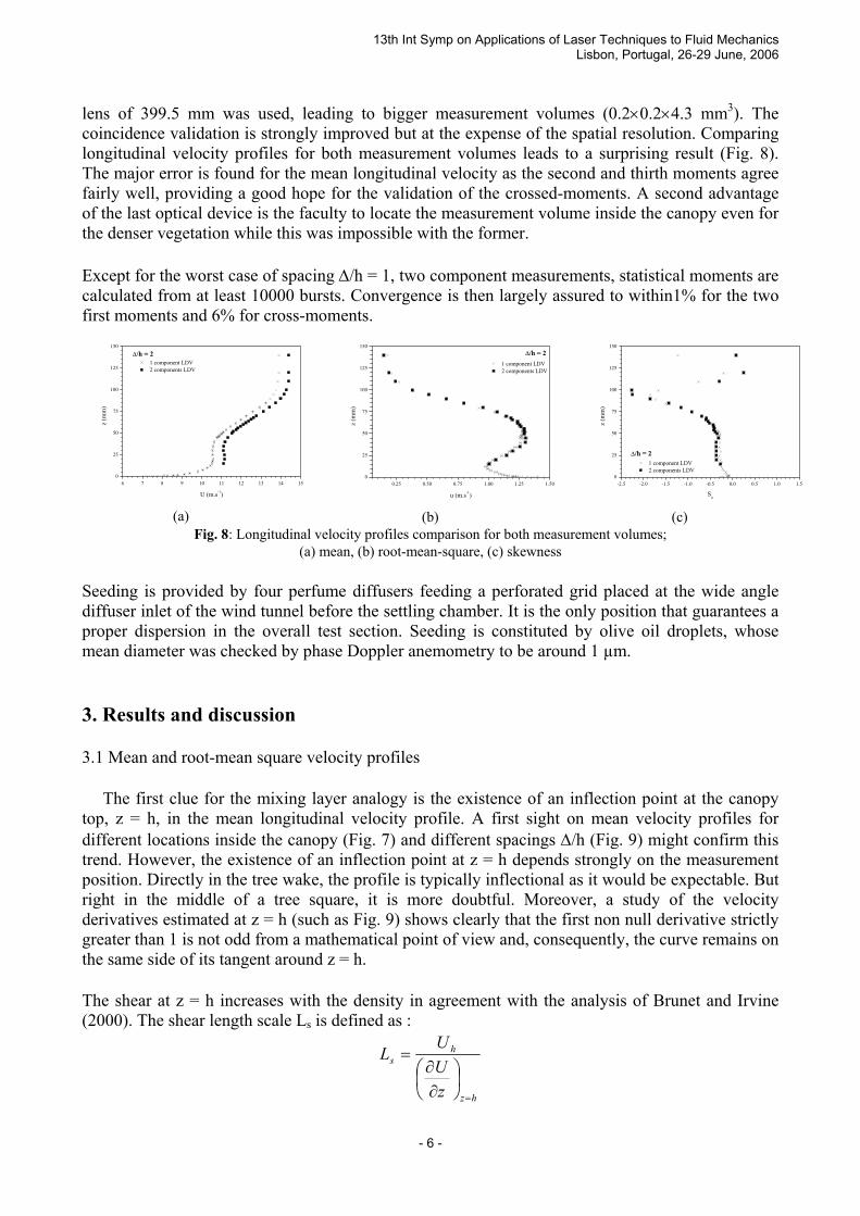
lens of 399.5 mm was used, leading to bigger measurement volumes (0.2×0.2×4.3 mm3). The coincidence validation is strongly improved but at the expense of the spatial resolution. Comparing longitudinal velocity profiles for both measurement volumes leads to a surprising result (Fig. 8). The major error is found for the mean longitudinal velocity as the second and thirth moments agree fairly well, providing a good hope for the validation of the crossed-moments. A second advantage of the last optical device is the faculty to locate the measurement volume inside the canopy even for the denser vegetation while this was impossible with the former. Except for the worst case of spacing ∆/h = 1, two component measurements, statistical moments are calculated from at least 10000 bursts. Convergence is then largely assured to within1% for the two first moments and 6% for cross-moments.

(a)

(b)

(c)

Fig. 8: Longitudinal velocity profiles comparison for both measurement volumes; (a) mean, (b) root-mean-square, (c) skewness

Seeding is provided by four perfume diffusers feeding a perforated grid placed at the wide angle diffuser inlet of the wind tunnel before the settling chamber. It is the only position that guarantees a proper dispersion in the overall test section. Seeding is constituted by olive oil droplets, whose mean diameter was checked by phase Doppler anemometry to be around 1 µm. 3. Results and discussion 3.1 Mean and root-mean square velocity profiles The first clue for the mixing layer analogy is the existence of an inflection point at the canopy top, z = h, in the mean longitudinal velocity profile. A first sight on mean velocity profiles for different locations inside the canopy (Fig. 7) and different spacings ∆/h (Fig. 9) might confirm this trend. However, the existence of an inflection point at z = h depends strongly on the measurement position. Directly in the tree wake, the profile is typically inflectional as it would be expectable. But right in the middle of a tree square, it is more doubtful. Moreover, a study of the velocity derivatives estimated at z = h (such as Fig. 9) shows clearly that the first non null derivative strictly greater than 1 is not odd from a mathematical point of view and, consequently, the curve remains on the same side of its tangent around z = h. The shear at z = h increases with the density in agreement with the analysis of Brunet and Irvine (2000). The shear length scale Ls is defined as :

hz

hs

zUUL

=

∂∂

=


- 7 -

This scale controls length scales in canopy flows and is similar to the half vorticity scale in mixing layers (Brunet and Irvine 2000). Ls decreases when canopies become denser and shear stronger. Ls/h varies between 0.1 and 0.85 for the relatively dense canopies mentioned by Finnigan (2000) while Brunet and Irvine found Ls/h equal to 0.1, 0.5 and 1 respectively for dense, moderate and sparse canopies in neutral atmospherical conditions. The trend is analogous for our data: Ls/h = 1.4, 2.2 and 3.9 respectively for ∆/h = 1, 1.5 and 2.

∆∆∆

Fig. 9: Longitudinal velocity mean profiles for three spacings ∆/h

Above z/h = 2.5, flow characteristics are those of the outer flow, in particular a very low turbulence intensity and no more shear. We thus restrict next graphs to ordinates lower than 2 because the trends above it are not very representative and literature data are usually limited to this height. Furthermore, we note here the greatest default of our study. As the basic flow in our wind tunnel is a turbulent boundary layer with a low turbulence intensity outer flow, all second order and higher order velocity moments become zero outside the boundary layer and then differ notably from actual atmospheric boundary layers and natural canopy flows.

For instance, root-mean square longitudinal component of the velocity, 212u

/ mentioned by simply

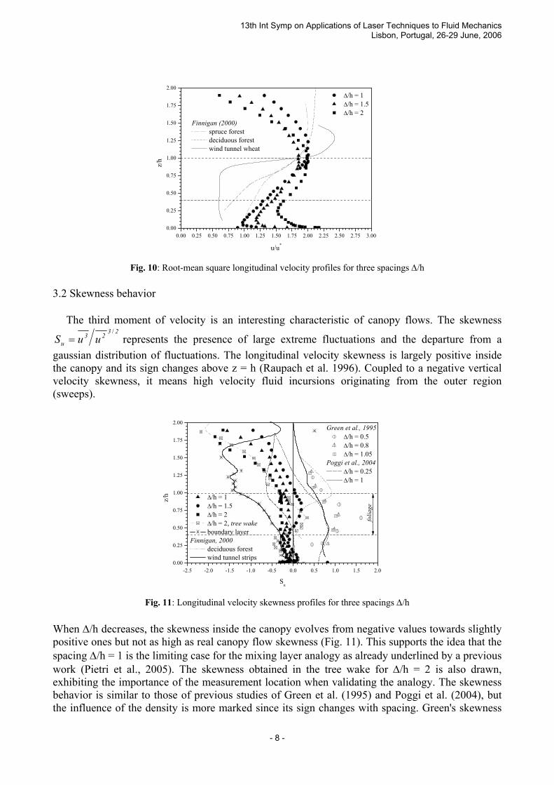
u in Fig. 10, when adimensionalized by the friction velocity whose estimation is explained §3.3, behaves similarly to the root-mean square of velocity typically found in canopies (Fig. 10) except in the outer region where the flow recovers the features of the boundary layer. Especially, we note just above the top of the foliage a zone of quasi constant value all the more pronounced that the spacing ∆/h is reduced. As Green et al. (1995) found, denser the canopy, lower the normalized standard deviation of longitudinal velocity inside the canopy. Except for the spacing ∆/h = 1.5, standard deviation is almost constant and equal to the classical value 2 at the upper part of the canopy and just above it. This suggests a surevaluation of the friction velocity u* for ∆/h = 1.5 although the Reynolds stress constant region was well-defined. Compared to Finnigan data reported in Fig. 10, a global reduction of the root-mean square velocity inside the canopy occurs when the canopy density raises.


- 8 -

Fig. 10: Root-mean square longitudinal velocity profiles for three spacings ∆/h

3.2 Skewness behavior The third moment of velocity is an interesting characteristic of canopy flows. The skewness

2323u uuS

/= represents the presence of large extreme fluctuations and the departure from a

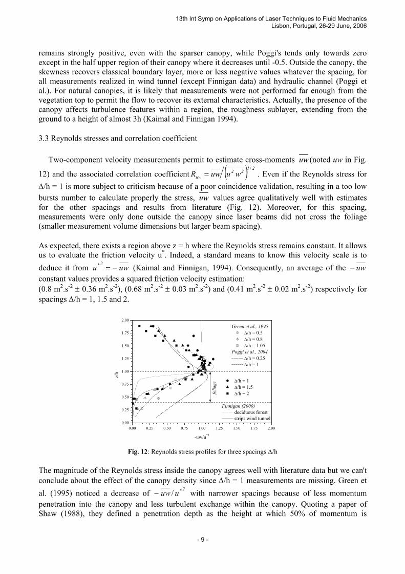
gaussian distribution of fluctuations. The longitudinal velocity skewness is largely positive inside the canopy and its sign changes above z = h (Raupach et al. 1996). Coupled to a negative vertical velocity skewness, it means high velocity fluid incursions originating from the outer region (sweeps).

Fig. 11: Longitudinal velocity skewness profiles for three spacings ∆/h

When ∆/h decreases, the skewness inside the canopy evolves from negative values towards slightly positive ones but not as high as real canopy flow skewness (Fig. 11). This supports the idea that the spacing ∆/h = 1 is the limiting case for the mixing layer analogy as already underlined by a previous work (Pietri et al., 2005). The skewness obtained in the tree wake for ∆/h = 2 is also drawn, exhibiting the importance of the measurement location when validating the analogy. The skewness behavior is similar to those of previous studies of Green et al. (1995) and Poggi et al. (2004), but the influence of the density is more marked since its sign changes with spacing. Green's skewness


- 9 -

remains strongly positive, even with the sparser canopy, while Poggi's tends only towards zero except in the half upper region of their canopy where it decreases until -0.5. Outside the canopy, the skewness recovers classical boundary layer, more or less negative values whatever the spacing, for all measurements realized in wind tunnel (except Finnigan data) and hydraulic channel (Poggi et al.). For natural canopies, it is likely that measurements were not performed far enough from the vegetation top to permit the flow to recover its external characteristics. Actually, the presence of the canopy affects turbulence features within a region, the roughness sublayer, extending from the ground to a height of almost 3h (Kaimal and Finnigan 1994). 3.3 Reynolds stresses and correlation coefficient Two-component velocity measurements permit to estimate cross-moments uw (noted uw in Fig.

12) and the associated correlation coefficient ( ) 2122uw wuuwR

/= . Even if the Reynolds stress for

∆/h = 1 is more subject to criticism because of a poor coincidence validation, resulting in a too low bursts number to calculate properly the stress, uw values agree qualitatively well with estimates for the other spacings and results from literature (Fig. 12). Moreover, for this spacing, measurements were only done outside the canopy since laser beams did not cross the foliage (smaller measurement volume dimensions but larger beam spacing). As expected, there exists a region above z = h where the Reynolds stress remains constant. It allows us to evaluate the friction velocity u*. Indeed, a standard means to know this velocity scale is to deduce it from uwu 2

−=* (Kaimal and Finnigan, 1994). Consequently, an average of the uw− constant values provides a squared friction velocity estimation: (0.8 m2.s-2 ± 0.36 m2.s-2), (0.68 m2.s-2 ± 0.03 m2.s-2) and (0.41 m2.s-2 ± 0.02 m2.s-2) respectively for spacings ∆/h = 1, 1.5 and 2.

Fig. 12: Reynolds stress profiles for three spacings ∆/h

The magnitude of the Reynolds stress inside the canopy agrees well with literature data but we can't conclude about the effect of the canopy density since ∆/h = 1 measurements are missing. Green et al. (1995) noticed a decrease of 2uuw */− with narrower spacings because of less momentum penetration into the canopy and less turbulent exchange within the canopy. Quoting a paper of Shaw (1988), they defined a penetration depth as the height at which 50% of momentum is


- 10 -

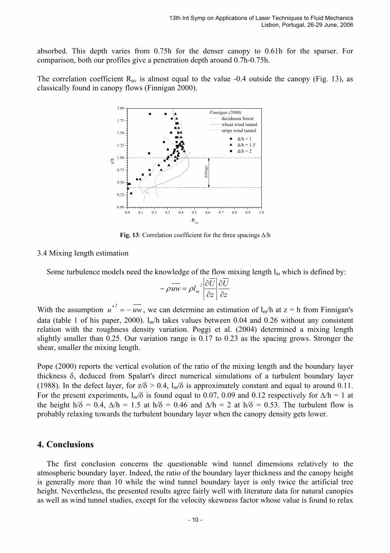
absorbed. This depth varies from 0.75h for the denser canopy to 0.61h for the sparser. For comparison, both our profiles give a penetration depth around 0.7h-0.75h. The correlation coefficient Ruv is almost equal to the value -0.4 outside the canopy (Fig. 13), as classically found in canopy flows (Finnigan 2000).

∆∆∆

Fig. 13: Correlation coefficient for the three spacings ∆/h

3.4 Mixing length estimation Some turbulence models need the knowledge of the flow mixing length lm which is defined by:

zU

zUluw 2

m ∂∂

∂∂

=− ρρ

With the assumption uwu 2−=* , we can determine an estimation of lm/h at z = h from Finnigan's

data (table 1 of his paper, 2000). lm/h takes values between 0.04 and 0.26 without any consistent relation with the roughness density variation. Poggi et al. (2004) determined a mixing length slightly smaller than 0.25. Our variation range is 0.17 to 0.23 as the spacing grows. Stronger the shear, smaller the mixing length. Pope (2000) reports the vertical evolution of the ratio of the mixing length and the boundary layer thickness δ, deduced from Spalart's direct numerical simulations of a turbulent boundary layer (1988). In the defect layer, for z/δ > 0.4, lm/δ is approximately constant and equal to around 0.11. For the present experiments, lm/δ is found equal to 0.07, 0.09 and 0.12 respectively for ∆/h = 1 at the height h/δ = 0.4, ∆/h = 1.5 at h/δ = 0.46 and ∆/h = 2 at h/δ = 0.53. The turbulent flow is probably relaxing towards the turbulent boundary layer when the canopy density gets lower. 4. Conclusions The first conclusion concerns the questionable wind tunnel dimensions relatively to the atmospheric boundary layer. Indeed, the ratio of the boundary layer thickness and the canopy height is generally more than 10 while the wind tunnel boundary layer is only twice the artificial tree height. Nevertheless, the presented results agree fairly well with literature data for natural canopies as well as wind tunnel studies, except for the velocity skewness factor whose value is found to relax


- 11 -

to the natural boundary layer value for z/h larger than 1.5. A departure from the mixing layer analogy is exhibited from the study of statistical moments of velocity. Comparisons concern measurements achieved in an intermediate position in the canopy where wake interactions seem to be less. Effectively, compared to tree wake mean velocity profiles, shear at z = h is attenuated, resulting in the disappearance of the inflectional point when density is reduced. The more sensitive turbulence parameter seems to be the velocity skewness inside the canopy going from classical positive values to negative ones, indicating the decrease of sweeps occurrence for wider canopies. Moreover, an estimation of the mixing length shows that the turbulent flow scales become more and more similar to those of a standard boundary layer when the canopy is sparser and sparser. However, the transition is not complete: the mean velocity profile for ∆/h = 2 is still far from typical boundary layer profiles. We modified here the canopy density by playing with element spacing. The canopy density will be changed too, using a different type of tree, characterized by different leaf area index, and/or with another element ground distribution (staggered configuration). Systematic measurements will be performed, providing data set with varying density. A synthetic analysis will then allow us to define the transition from the mixing layer analogy towards the perturbed boundary layer. References Brunet Y., Finnigan J.J., Raupach M.R. (1994) A wind tunnel study of air flow in waving wheat: single-point velocity statistics. Boundary-Layer Meteorol. 70:95-132 Brunet Y., Irvine M.R. (2000) The control of coherent eddies in vegetation canopies: streamwise structure spacing, canopy shear scale and atmospheric stability. Boundary-Layer Meteorol. 94:139-163 Cionco R.M. (1972) A wind-profile index for canopy flow. Boundary-Layer Meteorol. 3:255-263 Finnigan J.J. (2000) Turbulence in plant canopies. Ann. Rev. Fluid Mech. 32: 519-571 Green S. R., Grace J., Hutchings N. J. (1995) Observations of turbulent air flow in three stands of widely spaced Sitka spruce. Agric. For. Meteorol. 74 (3-4): 205-225 Kaimal J.C., Finnigan J.J. (1994) Atmospheric boundary layer flows. Their structure and measurement. pp 66-108 Oxford University Press Petroff A. (2005a), Mechanistic study of aerosol dry deposition on vegetated canopies. Radioprotection 40 (1): 443-450 Petroff A. (2005b) Etude mécaniste du dépôt sec d'aérosols sur les couverts végétaux. Thèse de l'Université d'Aix-Marseille II, France Pietri L., Amielh M., Anselmet F. (2005) Visualisations d'un écoulement turbulent autour d'un couvert végétal, FLUVISU 11, 7-9 juin, Lyon, France Poggi D., Porporato A., Ridolfi L., Albertson J.D., Katul G.G. (2004) The effect of vegetation density on canopy sub-layer turbulence. Boundary-Layer Meteorol. 111:565-587 Pope S. B. (2000) Turbulent flows. pp 307, Cambridge University Press Py C., de Langre E., Moulia B., Hémon P. (2005) Measurement of wind-induced motion of crop canopies from digital video images. Agric. For. Meteorol. 130: 223-236 Raupach M.R., Antonia R.A., Rajagoplan S. (1991) Rough-wall turbulent boundary layers. Appl Mech Rev 44 (1): 1-25 Raupach M.R., Finnigan J.J., Brunet Y. (1996) Coherent eddies in vegetation canopies : the mixing layer analogy. Boundary-Layer Meteorol., 78: 351-382

Effect of the vegetation density on the turbulence...

Documents

Transcript of Effect of the vegetation density on the turbulence...