Effect of Tack and Prime Coats, and Baghouse Fines on ...
213
Abstract KULKARNI, MORESHWAR BALAKRISHNA. Effect of Tack and Prime Coats, and Baghouse Fines on Composite Asphalt Pavements. (Under the direction of Dr. Akhtarhusein A. Tayebali.) This investigation was undertaken to develop a mechanistic design procedure to minimize the interfacial delamination distress, and to evaluate the contribution of baghouse fines to delamination in composite pavements. The need for this research was based on extensive occurrence of delamination problems in Division 13 of NCDOT. Pavements in Buncombe County, where emulsions were used as tack coat, had higher occurrence of such distresses compared to Rutherford County where PG64-22 binder was used as tack coat. In addition to use of tack coats, the asphalt mixes in these counties were prepared by an intermittent purging of baghouse fines. Results from particle analyzer indicated similar gradations for baghouse fines and regular mineral fillers. DSR testing of mastics indicated a similar performance of mastics prepared with regular fillers and baghouses. SST (FSCH and RSCH) and APA tests results on the mixtures with and without baghouse fines did not indicate a significant difference between the two mixes. However, AASHTO T283 test indicated that mixes with baghouse fines were moisture sensitive than mixes without baghouse fines. It could be possible that dosage of anti-strip additive might not have been adequate to counteract moisture damage. Composite AC-AC, AC-PCC and AC-CTB samples were fabricated in the laboratory and the interfacial bond strength was measured using the SST. For tack coats, it was observed that PG64-22 performed better on AC-AC interfaces, whereas CMS-2 performed
Transcript of Effect of Tack and Prime Coats, and Baghouse Fines on ...

Abstract KULKARNI, MORESHWAR BALAKRISHNA. Effect of Tack and Prime Coats, and
Baghouse Fines on Composite Asphalt Pavements. (Under the direction of Dr. Akhtarhusein
A. Tayebali.)
This investigation was undertaken to develop a mechanistic design procedure to
minimize the interfacial delamination distress, and to evaluate the contribution of baghouse
fines to delamination in composite pavements. The need for this research was based on
extensive occurrence of delamination problems in Division 13 of NCDOT. Pavements in
Buncombe County, where emulsions were used as tack coat, had higher occurrence of such
distresses compared to Rutherford County where PG64-22 binder was used as tack coat. In
addition to use of tack coats, the asphalt mixes in these counties were prepared by an
intermittent purging of baghouse fines.
Results from particle analyzer indicated similar gradations for baghouse fines and
regular mineral fillers. DSR testing of mastics indicated a similar performance of mastics
prepared with regular fillers and baghouses. SST (FSCH and RSCH) and APA tests results
on the mixtures with and without baghouse fines did not indicate a significant difference
between the two mixes. However, AASHTO T283 test indicated that mixes with baghouse
fines were moisture sensitive than mixes without baghouse fines. It could be possible that
dosage of anti-strip additive might not have been adequate to counteract moisture damage.
Composite AC-AC, AC-PCC and AC-CTB samples were fabricated in the laboratory
and the interfacial bond strength was measured using the SST. For tack coats, it was
observed that PG64-22 performed better on AC-AC interfaces, whereas CMS-2 performed

better on AC-PCC interface. CSS-1h performed better than EA-P and EPR-1 as a prime coat.
Non-bonded surfaces could not resist any interfacial shear.
Using a 3-D computer program, the interfacial shear stresses were computed at
various thickness, loading and temperature conditions. The results indicated that
delamination will not be a problem at lower temperature (20 °C), but at elevated
temperatures a minimum AC layer thickness is necessary to reduce the interfacial shear stress
to laboratory measured values. For thin pavement sections, the use of prime coat was
recommended to increase the bond between the AC and underlying layers.

EFFECT OF TACK AND PRIME COATS, AND BAGHOUSE FINES ON COMPOSITE ASPHALT PAVEMENTS
by
MORESHWAR BALAKRISHNA KULKARNI
A dissertation submitted to the Graduate Faculty of
North Carolina State University
in partial fulfillment of the requirements for the Degree of
Doctor of Philosophy
CIVIL ENGINEERING
Raleigh, North Carolina
April, 2004
Approved by:
____________________________ ____________________________
Dr. Y. Richard Kim Dr. Tasnim Hassan
____________________________ ____________________________
Dr. John W. Baugh, Jr. Dr. Akhtarhusein A. Tayebali
(Chair of Advisory Committee)

ii
Dedicated to my parents,
Mr. Balakrishna A. Kulkarni
And
Mrs. Swati B. Kulkarni,
And my sister,
Ms. Ratnamala B. Kulkarni

iii
Biography Moreshwar Kulkarni, son of Mr. Balakrishna Kulkarni and Ms. Swati Kulkarni, was
born on July 2, 1976, in Bombay, India. After finishing his high school education in 1993, he
joined the Indian Institute of Technology, Bombay (IIT Bombay) for Bachelors in Civil
Engineering. In fall 1997, after graduating from IIT Bombay, he joined the Master’s program
in Transportation Materials at North Carolina State University. During his MS at NC State,
he worked on pavement analysis, asphalt mix design, and performance evaluation of binders
and mixes. He graduated with a MS degree in summer 1999 and enrolled in the PhD program
in fall 1999. He served as a Departmental Ambassador for international students for
academic years from 2000-03. After graduation from NC State, he intends to pursue a career
in field of transportation engineering.

iv
Acknowledgments The author expresses his thanks to everyone that has been of assistance in the
experimental work and writing of this dissertation. Special thanks are due to Dr A. A.
Tayebali, graduate advisor, and Chairman of the advisory committee, for his guidance,
patience, help, and relentless support during my pursuit of doctoral degree. He has been a
mentor, an excellent teacher, and constant source of encouragement always eager to help. He
has been a great advisor, and his patience in going through versions of this dissertation,
various research reports, and several quarterly progress reports, is appreciated.
I am thankful to my committee members, Dr. Tasnim Hassan, Dr. Y. Richard Kim,
Dr. John W. Baugh, and Dr. R. Michael Young for their time, and evaluation of my work.
Thanks are also due to Dr. David W. Johnston, Director of Graduate Programs, for his help
and consideration. Dr. Michael Leming’s help in regard to design of PCC mixes and CTB
bases is appreciated. Dr. M. S. Rahman and Ms. Qingxia Xu’s assistance in the research
work related to this thesis is acknowledged.
Thanks are due to North Carolina Department of Transportation for their sponsorship
of this project. Mr. Christopher Bacchi, M&T unit NCDOT, has been of immense help
answering our queries and helping us with material procurement.
It was fun rolling and coring slabs with Kevin Fischer, my fellow graduate student. I
truly enjoyed your company while working and appreciate your help. Thanks are due to
Yuanxiong Huang and Prasad Kollipara for their assistance in fabricating samples. Steven
Wade, departmental mechanic, has been helpful in fabrication of molds for slab construction,
and repairing of the rolling wheel compactor.
During my assignment to the Graduate Programs office, interaction with Renee
Howard and Edna White was enjoyable. I relished working on those ‘orange folders’ very
much. I wish to mention Ms. Barbara Nicholson from Civil Engineering main office for her
help in administrative matters. I would take this opportunity to say hello to my current and
former colleagues from room 401 and asphalt lab: Priya Nimbole, Suriyan Sadasivam, Dr.
Glen Malpass, Hazim Dwairi, Dr. Bing Xu, Dr. Jo Daniel, Dr. Yanqing Zhao, Dr. Haifang

v
Wen, Dr. Sungho Mun, Mark King, Shane Underwood, Mostafa Momen, and Dr. Ghassan
Chehab. Thanks are due to Balaji Iyengar for his help in troubleshooting computers and
printers, as well as keeping the systems up to date.
It was an excellent six and half year sojourn in the US. I truly enjoyed the time spent
on and off campus. Dr. Gajanan Natu and his wife, Vijaya, have been supportive and helpful
during some of my most trying times. I am grateful to them for their support. These
acknowledgements would not be complete without a mention of my friends from my alma
mater, IIT Bombay, responsible for maxing out my cellular night and weekend minutes. I
enjoyed having conversations with you all – Dr. Atul Karve, Amitkumar Rao, Anupkumar
Rao, Babu Mamidipally, Nagendra Jain, Manish Goyal, Anurag Pareek, and Dr. Durgaprasad
Shamain – and thanks for your support. I would like to mention Anuja Shukla for her
encouragement, advice and interesting conversations.
Thank you to Amit Kulkarni, Ajit Moghe, Chirag Modi, Sirish Somanchi, Devarajan
Balaraman, Kesava Narasimhan, Rahul Vallabh, and Pankaj Agrawal for putting up with me
as a roommate. Thanks are due to Dibyendu Sengupta for his continuous insight and
encouragement in my ongoing job search. I would like to take this opportunity to thank my
physicians Drs. Michael Dewitt, Laura Pratt, and Shawn Phelan.
Last but not the least, I would like to express my indebtedness to my parents and my
sister for pushing me to undertake and complete this mission; without your unwavering
support this would not have been possible. It has been a dream comes true for all of us.

vi
Table of Contents
LIST OF TABLES………………………………………………...…………………...…………………..........ix
LIST OF FIGURES…………….......…………………..………………………………………………………xi
LIST OF ABBREVIATIONS AND SYMBOLS……………………………………………………………..xv
1 INTRODUCTION AND LITERATURE SURVEY ................................................................................1 1.1 INTRODUCTION.....................................................................................................................................1 1.2 LITERATURE SURVEY...........................................................................................................................3
1.2.1 Study by Mohammad et al [18] ......................................................................................................3 1.2.2 Study by Shahin et al [21] ..............................................................................................................4 1.2.3 Study by Uzan et al [30, 31] ...........................................................................................................5 1.2.4 Study by Tschegg et al [29] ............................................................................................................7 1.2.5 Study by Ameri-Gaznon et al [6] ....................................................................................................8 1.2.6 Study by Ishai et al [15]................................................................................................................10 1.2.7 Study by Hachiya et al [12] ..........................................................................................................11 1.2.8 Study by Mukhtar et al [19]..........................................................................................................13 1.2.9 Study by Sholar et al [24].............................................................................................................13 1.2.10 Prime Coats .............................................................................................................................14 1.2.11 Tack Coats ...............................................................................................................................15
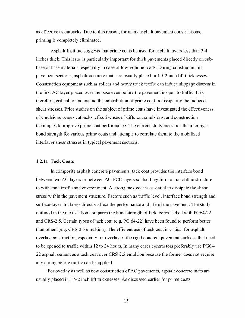
1.3 RESEARCH NEED................................................................................................................................16 1.3.1 Prior Work....................................................................................................................................16
2 RESEARCH APPROACH AND METHODOLOGY ...........................................................................19 2.1 OBJECTIVE .........................................................................................................................................19 2.2 RESEARCH METHODOLOGY ...............................................................................................................19
2.2.1 Literature Review and Survey.......................................................................................................19 2.2.2 Asphalt and Mastics Testing.........................................................................................................20 2.2.3 SST Testing of SGC Specimens, TSR and APA Tests....................................................................20 2.2.4 Material Characterization ............................................................................................................21 2.2.5 Fabrication of Slabs and Test Specimens .....................................................................................21 2.2.6 Bond Strength Determination using Shear Testing.......................................................................21 2.2.7 Mechanistic Analysis ....................................................................................................................22
3 SURVEY RESULTS.................................................................................................................................24 3.1 DEVELOPMENT OF QUESTIONNAIRE ...................................................................................................24 3.2 SURVEY RESPONSES...........................................................................................................................24
4 RHEOLOGICAL EVALUATION..........................................................................................................28 4.1 INTRODUCTION...................................................................................................................................28 4.2 SELECTION OF FINES ..........................................................................................................................28 4.3 GRADATION ANALYSIS OF FINES USING FHWA PARTICLE ANALYZER..............................................29
4.3.1 Method Description ......................................................................................................................29 4.3.2 Results and Discussion .................................................................................................................29
4.4 ANALYSIS OF ASPHALT-FINES MASTICS USING DSR .........................................................................30 4.4.1 Specimen Preparation ..................................................................................................................31 4.4.2 Test Parameters............................................................................................................................31 4.4.3 Test Results and Discussion..........................................................................................................32
4.5 DSR TESTING OF EMULSIONS ............................................................................................................33

vii
4.5.1 Test Results and Discussion..........................................................................................................34 4.6 BROOKFIELD VISCOSITY ....................................................................................................................35 4.7 CONCLUSIONS ....................................................................................................................................35
5 PERFORMANCE TESTING OF SGC SPECIMENS...........................................................................45 5.1 INTRODUCTION...................................................................................................................................45 5.2 TEST PARAMETERS ............................................................................................................................45 5.3 TEST TEMPERATURE ..........................................................................................................................46
5.3.1 Selection of Testing Temperature .................................................................................................46 5.3.2 Temperature Zones .......................................................................................................................46 5.3.3 Selection of Depth for Computation of Testing Temperature .......................................................47 5.3.4 Reliability Factors ........................................................................................................................47 5.3.5 Temperature Selection Method.....................................................................................................47
5.4 PERFORMANCE TEST RESULTS OF LAB MIXES WITH BAGHOUSE FINES .............................................48 5.4.1 Specimen Fabrication...................................................................................................................48 5.4.2 FSCH Test ....................................................................................................................................49 5.4.3 RSCH Test ....................................................................................................................................50
5.5 ASPHALT PAVEMENT ANALYZER TESTS ............................................................................................51 5.5.1 APA Test Results...........................................................................................................................52
5.6 EFFECT OF BAGHOUSE FINES ON MOISTURE SENSITIVITY..................................................................53 5.7 SUMMARY AND CONCLUSION ............................................................................................................53
6 SPECIMEN FABRICATION USING ROLLING WHEEL COMPACTOR .....................................64 6.1 INTRODUCTION...................................................................................................................................64 6.2 FABRICATION OF STEEL MOLDS.........................................................................................................64 6.3 SPECIMEN FABRICATION ....................................................................................................................65
6.3.1 Asphalt Concrete Slabs.................................................................................................................65 6.3.2 Portland Cement Concrete Slabs..................................................................................................66 6.3.3 Cement Treated Base Slab............................................................................................................66
6.4 TACK / PRIME COAT APPLICATION.....................................................................................................67 6.5 CORING AND CUTTING SAMPLES........................................................................................................68
7 MATERIAL CHARACTERIZATION...................................................................................................76 7.1 INTRODUCTION...................................................................................................................................76 7.2 ASPHALT MIX CHARACTERIZATION...................................................................................................76
7.2.1 Frequency Sweep Test at Constant Height (FSCH)......................................................................77 7.2.2 Repeated Shear Test at Constant Height (RSCH).........................................................................78 7.2.3 Axial Frequency Sweep Test (AFST) ............................................................................................78 7.2.4 Repeated Axial Test ......................................................................................................................79
7.3 PORTLAND CEMENT CONCRETE (PCC) CHARACTERIZATION.............................................................80 7.3.1 Mixing, Casting and Curing of Specimens ...................................................................................80 7.3.2 Compressive Strength of Cylindrical Concrete Specimens...........................................................82 7.3.3 Modulus of Rupture for Concrete Specimens ...............................................................................83 7.3.4 Splitting Tension Test for Concrete Specimens ............................................................................83 7.3.5 Elastic Modulus Test for Concrete Specimens..............................................................................83
7.4 CEMENT TREATED BASE (CTB) CHARACTERIZATION .......................................................................84 7.4.1 CTB Composition .........................................................................................................................84 7.4.2 Atterberg Limits for CTB Aggregates...........................................................................................85 7.4.3 Modified Proctor Density Test......................................................................................................85
8 BOND STRENGTH DETERMINATION............................................................................................107 8.1 INTRODUCTION.................................................................................................................................107
8.1.1 Shear Test Description ...............................................................................................................107 8.2 BOND STRENGTH USING METAL PLATENS .......................................................................................108 8.3 BOND STRENGTH OF AC-AC SPECIMENS .........................................................................................109
8.3.1 Axial and Shear Ramp Test.........................................................................................................109

viii
8.3.2 Axial Test Results........................................................................................................................110 8.3.3 Shear Test Results.......................................................................................................................110
8.4 BOND STRENGTH OF PCC-AC SPECIMENS .......................................................................................112 8.5 BOND STRENGTH OF CTB-AC SPECIMENS .......................................................................................114 8.6 SUMMARY AND CONCLUSIONS.........................................................................................................116
9 DEVELOPMENT OF DESIGN GUIDELINES FOR USE OF TACK AND PRIME COATS .......136 9.1 3-D LAYERED ELASTIC PROGRAM DESCRIPTION .............................................................................136 9.2 LOAD CONDITIONS...........................................................................................................................137 9.3 TEMPERATURE EFFECTS...................................................................................................................138 9.4 ANALYSIS OF AC-AC BONDING.......................................................................................................139 9.5 ANALYSIS OF PCC-AC BONDING.....................................................................................................140 9.6 ANALYSIS OF CTB-AC BONDING ....................................................................................................141 9.7 OUTLINE OF GUIDELINE DEVELOPMENT FOR USE OF TACK OR PRIME COAT ...................................142 9.8 SUMMARY AND CONCLUSIONS.........................................................................................................143
10 SUMMARY, CONCLUSIONS AND RECOMMENDATIONS.........................................................151 10.1 SUMMARY AND CONCLUSIONS.........................................................................................................151 10.2 FUTURE SCOPE.................................................................................................................................156
11 REFERENCES........................................................................................................................................158 APPENDIX A…………………………………………………………….……………………..……………..162
APPENDIX B………………………………………………………………………………………………….164
APPENDIX C…………………………………………………………………………………...……………..170
APPENDIX D………………………………………………………………………………………………….174
APPENDIX E………………………………………………………………………………………………….179
APPENDIX F………………………………………………………………………………………………….189

ix
List of Tables
TABLE 4-1 PROPERTIES OF FINES FROM PARTICLE SIZE ANALYSIS (SET 2) [13]......................................................36 TABLE 4-2 TEMPERATURES FOR RESIDUAL BINDERS WHEN |G*|/SINδ ≥ 1.0 KPA ...................................................36 TABLE 5-1 AIR VOIDS AND GMM OF 150-MM DIAMETER LABORATORY MIX SPECIMENS .........................................54 TABLE 5-2 NATIONWIDE PAVEMENT TEMPERATURES, [23] ...................................................................................54 TABLE 5-3 AVERAGE DEPTHS AND TEST TEMPERATURES ......................................................................................55 TABLE 5-4 |G*| (PA) VERSUS FREQUENCY (HZ) FOR LAB MIXES, 50.2 °C, BUNCOMBE COUNTY ...........................55 TABLE 5-5 δ (DEGREES) VERSUS FREQUENCY (HZ) FOR LAB MIXES, 50.2 °C, BUNCOMBE COUNTY ......................55 TABLE 5-6 AVERAGE |G*|, δ, AND |G*|/SIN δ VALUES, 50.2 °C, LAB MIXES BUNCOMBE COUNTY.........................56 TABLE 5-7 |G*| (PA) VERSUS FREQUENCY (HZ) FOR LAB MIXES, 50.2 °C, RUTHERFORD COUNTY ........................56 TABLE 5-8 δ (DEGREES) VERSUS FREQUENCY (HZ) FOR LAB MIXES, 50.2 °C, RUTHERFORD COUNTY...................56 TABLE 5-9 AVERAGE |G*|, δ, AND |G*|/SIN δ VALUES, 50.2 °C, LAB MIXES RUTHERFORD COUNTY......................57 TABLE 5-10 STRAIN AT THE END OF RSCH TEST, 50.2 °C, LAB MIXES ..................................................................57 TABLE 5-11 AIR VOIDS AND HEIGHTS OF 6-INCH DIAMETER LABORATORY SPECIMENS FOR APA TEST .................57 TABLE 5-12 BUNCOMBE COUNTY (WITH BAGHOUSE FINES) TSR RESULTS (4-INCH SPECIMENS)..........................57 TABLE 5-13 BUNCOMBE COUNTY (W/OUT BAGHOUSE FINES) TSR RESULTS (4-INCH SPECIMENS) .......................58 TABLE 5-14 RUTHERFORD COUNTY (WITH BAGHOUSE FINES) TSR RESULTS (4-INCH SPECIMENS) ......................58 TABLE 5-15 RUTHERFORD COUNTY (W/OUT BAGHOUSE FINES) TSR RESULTS (4-INCH SPECIMENS) ....................58 TABLE 5-16 SUMMARY OF TSR RESULTS ..............................................................................................................58 TABLE 7-1 AIR VOIDS OF AC MIX SAMPLES ..........................................................................................................86 TABLE 7-2 |G*| VS. FREQUENCY FOR AC MIX, 20 °C, IN PA...................................................................................86 TABLE 7-3 SHEAR PHASE ANGLE (DEGREES) VS. FREQUENCY FOR AC MIX, 20 °C.................................................87 TABLE 7-4 |G*| VS. FREQUENCY FOR AC MIX, 30 °C, IN PA...................................................................................87 TABLE 7-5 SHEAR PHASE ANGLE (DEGREES) VS. FREQUENCY FOR AC MIX, 30 °C.................................................87 TABLE 7-6 |G*| VS. FREQUENCY FOR AC MIX, 40 °C, IN PA...................................................................................88 TABLE 7-7 SHEAR PHASE ANGLE (DEGREES) VS. FREQUENCY FOR AC MIX, 40 °C.................................................88 TABLE 7-8 |G*| VS. FREQUENCY FOR AC MIX, 60 °C, IN PA...................................................................................88 TABLE 7-9 SHEAR PHASE ANGLE (DEGREES) VS. FREQUENCY FOR AC MIX, 60 °C.................................................89 TABLE 7-10 RSCH CYCLES, AT 40 AND 60 °C.......................................................................................................89 TABLE 7-11 AIR VOIDS OF AXIAL TEST SAMPLES...................................................................................................89 TABLE 7-12 |E*| VS. FREQUENCY FOR AC MIX, 20 AND 30 °C, IN PA.....................................................................89 TABLE 7-13 AXIAL PHASE ANGLE (DEGREES) VS. FREQUENCY FOR AC MIX, 20 AND 30 °C...................................90 TABLE 7-14 |E*| VS. FREQUENCY FOR AC MIX, 40 AND 60 °C, IN PA.....................................................................90
x
TABLE 7-15 AXIAL PHASE ANGLE (DEGREES) VS. FREQUENCY FOR AC MIX, 40 AND 60 °C...................................90 TABLE 7-16 REPEATED AXIAL TEST CYCLES, AT 40 AND 60 °C .............................................................................90 TABLE 7-17 AGGREGATE MOISTURE CONTENTS AND SPECIFIC GRAVITIES ............................................................91 TABLE 7-18 BATCH WEIGHTS FOR PCC.................................................................................................................91 TABLE 7-19 PROPERTIES OF CONCRETE.................................................................................................................91 TABLE 7-20 ELASTIC MODULUS FOR PCC.............................................................................................................91 TABLE 7-21 GRADATION (% PASSING) FOR AGGREGATE PILES USED FOR CTB .....................................................92 TABLE 7-22 GRADATION CRITERIA FOR MATERIAL PASSING #10 SIEVE (SOIL MORTAR)........................................92 TABLE 7-23 MOISTURE DENSITY DETERMINATION FOR CTB ................................................................................92 TABLE 7-24 LIQUID LIMIT PROPERTY FOR CTB USING DOT MODIFIED METHOD...................................................92 TABLE 8-1 RESULTS FOR AC-AC AXIAL RAMP TESTS (TENSILE), 40 °C ..............................................................117 TABLE 8-2 RESULTS FOR AC-AC AXIAL RAMP TESTS (TENSILE), 60 °C ..............................................................117 TABLE 8-3 RESULTS FOR AC-AC SHEAR RAMP TESTS, 20 °C..............................................................................117 TABLE 8-4 RESULTS FOR AC-AC SHEAR RAMP TESTS, 40 °C..............................................................................118 TABLE 8-5 RESULTS FOR AC-AC SHEAR RAMP TESTS, 60 °C..............................................................................118 TABLE 8-6 SUMMARY OF SHEAR STRENGTHS FROM SHOLAR ET AL, [24] ............................................................118 TABLE 8-7 RESULTS FOR PCC-AC SHEAR RAMP TESTS, 20 °C............................................................................119 TABLE 8-8 RESULTS FOR PCC-AC SHEAR RAMP TESTS, 40 °C............................................................................119 TABLE 8-9 RESULTS FOR PCC-AC SHEAR RAMP TESTS, 60 °C............................................................................119 TABLE 8-10 SUMMARY OF PCC-AC BOND STRENGTHS, [19] ..............................................................................120 TABLE 8-11 RESULTS FOR CTB-AC SHEAR RAMP TESTS, 40 °C..........................................................................120 TABLE 8-12 RESULTS FOR CTB-AC SHEAR RAMP TESTS, 60 °C..........................................................................120 TABLE 9-1 RECOMMENDED MINIMUM SKID NUMBERS FOR RURAL HIGHWAYS [16].............................................144 TABLE 9-2 INTERFACIAL SHEAR BOND STRENGTH SUMMARY FOR PG64-22 AND CMS-2 ...................................144 TABLE 9-3 AC-CTB SHEAR BOND STRENGTH SUMMARY FOR CSS-1H, EA-P, AND EPR-1 .................................144

xi
List of Figures
FIGURE 1-1 DELAMINATION OF SURFACE COURSE (SOURCE:
HTTP://WWW.KOCHPAVEMENTSOLUTIONS.COM/DISTRESSES/PUSHING.HTM).................................................2 FIGURE 1-2 DELAMINATION, EXPOSURE OF UNDERLYING LAYER (SRC:
HTTP://WWW.DEFENCE.GOV.AU/DEMG/7TECHNICAL_GUIDANCE/AIRCRAFT_PAVEMENT_MANUAL/PART_A/A
4.HTM)...........................................................................................................................................................2 FIGURE 1-3 DISTORTION AND SHOVING, DEFORMATION OF SURFACE LAYER UNDER LOAD (SRC:
HTTP://WWW.DEFENCE.GOV.AU/DEMG/7TECHNICAL_GUIDANCE/AIRCRAFT_PAVEMENT_MANUAL/PART_A/A
4.HTM)...........................................................................................................................................................2 FIGURE 1-4 TYPICAL SLIPPAGE FAILURE [11, 19] ....................................................................................................3 FIGURE 1-5 COLLARS DESIGNED FOR TESTING SAMPLES IN SHEAR, [18]..................................................................4 FIGURE 1-6 SCHEMATIC OF SPECIMEN DEFORMATION DURING SHEAR TESTING, [31] ..............................................7 FIGURE 1-7 SPECIMEN SHAPES FOR WEDGE SPLITTING TESTS, [29]..........................................................................9 FIGURE 1-8 SETUP OF WEDGE SPLITTING TEST, [29] ................................................................................................9 FIGURE 1-9 SPECIMEN SHAPES AND TESTING METHOD, [12]..................................................................................12 FIGURE 1-10 SHEAR TEST ON EMULSIONS, [12] .....................................................................................................12 FIGURE 1-11 SPECIMENS WITH TACK COAT AT INTERFACE, [19]............................................................................13 FIGURE 1-12 SHEARING DEVICE DEVELOPED BY SHOLAR ET AL [24] ....................................................................14 FIGURE 2-1 SUMMARY OF RESEARCH OUTLINE AND METHODOLOGY ....................................................................23 FIGURE 4-1 GRADATION ANALYSIS OF FINES USING FHWA PARTICLE ANALYZER, SET 2......................................37 FIGURE 4-2 GRADATION ANALYSIS OF FINES USING FHWA PARTICLE ANALYZER, SET 1......................................37 FIGURE 4-3 MASTER CURVES (|G*|) FOR BUNCOMBE COUNTY, 64 °C...................................................................38 FIGURE 4-4 MASTER CURVES (|G*|) FOR RUTHERFORD COUNTY, 64 °C ...............................................................38 FIGURE 4-5 MASTER CURVES (|G*|/SIN δ) FOR BUNCOMBE COUNTY, UNAGED, 64 OC...........................................39 FIGURE 4-6 MASTER CURVES (|G*|/SIN δ) FOR BUNCOMBE COUNTY, AGED, 64 OC ...............................................39 FIGURE 4-7 MASTER CURVES (|G*|/SIN δ) FOR RUTHERFORD COUNTY, UNAGED, 64 OC .......................................40 FIGURE 4-8 MASTER CURVES (|G*|/SIN δ) FOR RUTHERFORD COUNTY, AGED, 64 OC ............................................40 FIGURE 4-9 COMPARISON OF |G*|/SIN δ AT VARIOUS TEMPERATURES FOR RESIDUAL BINDERS .............................41 FIGURE 4-10 COMPARISON OF |G*| AT VARIOUS TEMPERATURES FOR RESIDUAL BINDERS ....................................41 FIGURE 4-11 COMPARISON OF δ AT VARIOUS TEMPERATURES FOR RESIDUAL BINDERS.........................................42 FIGURE 4-12 VISCOSITY VS. RPM, 150 °C ............................................................................................................42 FIGURE 4-13 PERCENT TORQUE VS. RPM, 150 °C.................................................................................................43 FIGURE 4-14 VISCOSITY VS. RPM, 135 °C ............................................................................................................43

xii
FIGURE 4-15 PERCENT TORQUE VS. RPM, 135 °C.................................................................................................44 FIGURE 5-1 NINE CLIMATIC REGIONS IN US ..........................................................................................................59 FIGURE 5-2 DYNAMIC SHEAR MODULUS (|G*|) VS. FREQ., 50.2 °C, BUNCOMBE, LAB MIXES ................................59 FIGURE 5-3 PHASE ANGLE (δ) VERSUS FREQUENCY, 50.2 °C, BUNCOMBE, LAB MIXES..........................................60 FIGURE 5-4 AVERAGE |G*| AND δ VALUES VS. FREQ., 50.2 °C, BUNCOMBE, LAB MIXES........................................60 FIGURE 5-5 DYNAMIC SHEAR MODULUS (|G*|) VS. FREQ., 50.2 °C, RUTHERFORD, LAB MIXES.............................61 FIGURE 5-6 PHASE ANGLE (δ) VS. FREQUENCY, 50.2 °C, RUTHERFORD, LAB MIXES..............................................61 FIGURE 5-7 AVERAGE |G*| AND δ VALUES VS. FREQ., 50.2 °C, RUTHERFORD, LAB MIXES.....................................62 FIGURE 5-8 PLASTIC SHEAR STRAIN VS. RSCH CYCLES, 50.2 °C, BUNCOMBE COUNTY, LAB MIXES.....................62 FIGURE 5-9 PLASTIC SHEAR STRAIN VS. RSCH CYCLES, 50.2 °C, RUTHERFORD COUNTY, LAB MIXES..................63 FIGURE 6-1 VIEW OF MOLD WITH ADJUSTABLE RAMPS (ON LEFT) .........................................................................69 FIGURE 6-2 MOLD WITH ROLLER...........................................................................................................................69 FIGURE 6-3 FRESHLY CAST PCC SLAB ..................................................................................................................70 FIGURE 6-4 SIDE VIEW WITH ROLLER ON THE MOLD..............................................................................................70 FIGURE 6-5 PHOTO OF A 1-INCH THICK CTB ‘DISK’ ..............................................................................................71 FIGURE 6-6 CTB ‘DISKS’ COATED WITH EMULSION...............................................................................................71 FIGURE 6-7 MOLD TOP – PART I ...........................................................................................................................72 FIGURE 6-8 MOLD BOTTOM – PART I ....................................................................................................................73 FIGURE 6-9 MOLD TOP – PART II ..........................................................................................................................74 FIGURE 6-10 MOLD BOTTOM – PART II.................................................................................................................75 FIGURE 7-1 DYNAMIC SHEAR MODULUS (|G*|) VS. FREQUENCY FOR AC MIX, 20 °C.............................................93 FIGURE 7-2 SHEAR PHASE ANGLE (δ) VS. FREQUENCY FOR AC MIX, 20 °C............................................................93 FIGURE 7-3 DYNAMIC SHEAR MODULUS (|G*|) VS. FREQUENCY FOR AC MIX, 30 °C.............................................94 FIGURE 7-4 SHEAR PHASE ANGLE (δ) VS. FREQUENCY FOR AC MIX, 30 °C............................................................94 FIGURE 7-5 DYNAMIC SHEAR MODULUS (|G*|) VS. FREQUENCY FOR AC MIX, 40 °C.............................................95 FIGURE 7-6 SHEAR PHASE ANGLE (δ) VS. FREQUENCY FOR AC MIX, 40 °C............................................................95 FIGURE 7-7 DYNAMIC SHEAR MODULUS (|G*|) VS. FREQUENCY FOR AC MIX, 60 °C.............................................96 FIGURE 7-8 SHEAR PHASE ANGLE (δ) VS. FREQUENCY FOR AC MIX, 60 °C............................................................96 FIGURE 7-9 AVERAGE DYNAMIC SHEAR MODULUS (|G*|) VS. FREQUENCY FOR AC MIX........................................97 FIGURE 7-10 AVERAGE SHEAR PHASE ANGLE (δ) VS. FREQUENCY FOR AC MIX ....................................................97 FIGURE 7-11 |G*| MASTER CURVE FOR AC MIX, 30 °C ..........................................................................................98 FIGURE 7-12 SHEAR PHASE ANGLE (δ) MASTER CURVE FOR AC MIX, 30 °C ..........................................................98 FIGURE 7-13 |G*| MASTER CURVE FOR AC MIX, 40 °C ..........................................................................................99 FIGURE 7-14 SHEAR PHASE ANGLE (δ) MASTER CURVE FOR AC MIX, 40 °C ..........................................................99 FIGURE 7-15 |G*| MASTER CURVE FOR AC MIX, 30 AND 40 °C............................................................................100 FIGURE 7-16 SHEAR PHASE ANGLE (δ) MASTER CURVE FOR AC MIX, 30 AND 40 °C............................................100

xiii
FIGURE 7-17 PLASTIC SHEAR STRAIN VS. RSCH CYCLES, 40 AND 60 °C FOR AC MIXES .....................................101 FIGURE 7-18 DYNAMIC AXIAL MODULUS (|E*|) VS. FREQUENCY FOR AC MIX.....................................................101 FIGURE 7-19 AVERAGE DYNAMIC AXIAL MODULUS (|E*|) VS. FREQUENCY FOR AC MIX.....................................102 FIGURE 7-20 AVERAGE AXIAL PHASE ANGLE (δ) VS. FREQUENCY FOR AC MIX...................................................102 FIGURE 7-21 PLASTIC AXIAL STRAIN VS. CYCLES, 40 AND 60 °C FOR AC MIXES.................................................103 FIGURE 7-22 RELATIONSHIP BETWEEN |G*| AND |E*| FOR AC MIXES ..................................................................103 FIGURE 7-23 RELATIONSHIP BETWEEN SHEAR AND AXIAL PHASE ANGLE FOR AC MIXES ....................................104 FIGURE 7-24 SET UP FOR ELASTIC MODULUS OF CONCRETE USING A 6×12 CYLINDER .........................................104 FIGURE 7-25 AXIAL STRESS VS. STRAIN AT 7 DAYS FOR PCC..............................................................................105 FIGURE 7-26 GRADATION OF MATERIALS USED FOR CTB ...................................................................................105 FIGURE 7-27 MOISTURE DENSITY CURVE FOR CTB.............................................................................................106 FIGURE 7-28 RESILIENT MODULUS OF CEMENT TREATED BASES (CTB), [1, 14] ..................................................106 FIGURE 8-1 DEBONDED COMPOSITE AC-AC SLAB WITHOUT TACK COAT............................................................121 FIGURE 8-2 AXIAL FAILURE OF CMS-2 SPECIMEN (C4 6-3-2) AT 2.5 MM/MIN, 40 °C..........................................121 FIGURE 8-3 AXIAL FAILURE OF CMS-2 SPECIMEN (C4 6-3-2) AT 2.5 MM/MIN, 40 °C..........................................122 FIGURE 8-4 AXIAL FAILURE OF PG64-22 SPECIMEN (M1 5-16-2) AT 2.5 MM/MIN, 40 °C ....................................122 FIGURE 8-5 AXIAL FAILURE OF PG64-22 SPECIMEN (M1 5-16-2) AT 2.5 MM/MIN, 40 °C ....................................123 FIGURE 8-6 AVERAGE SHEAR STRESS VS. TIME FOR AC-AC INTERFACE TACKED WITH CMS-2 ..........................123 FIGURE 8-7 AVERAGE SHEAR STRESS VS. TIME FOR AC-AC INTERFACE TACKED WITH PG64-22 .......................124 FIGURE 8-8 SUMMARY OF BOND STRENGTHS FOR AC-AC INTERFACE ................................................................124 FIGURE 8-9 SHEAR FAILURE OF CMS-2 SPECIMEN (M1 6-16-2) AT 1.0MM/MIN, 40 °C ........................................125 FIGURE 8-10 SHEAR FAILURE OF CMS-2 SPECIMEN (M3 6-3-2) AT 1.0MM/MIN, 40 °C ........................................125 FIGURE 8-11 SHEAR FAILURE OF CMS-2 SPECIMEN (C1 6-3-2) AT 2.5MM/MIN, 40 °C.........................................126 FIGURE 8-12 SHEAR FAILURE OF PG64-22 SPECIMEN (M1 5-7-2) AT 2.5 MM/MIN, 40 °C.....................................126 FIGURE 8-13 SHEAR FAILURE OF PG64-22 SPECIMEN (1MMC2_1) AT 1.0 MM/MIN, 20 °C ...................................127 FIGURE 8-14 SHEAR FAILURE OF PG64-22 SPECIMEN (25MMM3) AT 2.5 MM/MIN, 20 °C ....................................127 FIGURE 8-15 DEBONDING OF COMPOSITE PCC-AC SPECIMEN WITHOUT TACK COAT..........................................128 FIGURE 8-16 DEBONDED COMPOSITE PCC-AC SLABS WITHOUT TACK COAT......................................................128 FIGURE 8-17 AVERAGE SHEAR STRESS VS. TIME FOR PCC-AC INTERFACE TACKED WITH CMS-2 ......................129 FIGURE 8-18 AVERAGE SHEAR STRESS VS. TIME FOR PCC-AC INTERFACE TACKED WITH PG64-22 ...................129 FIGURE 8-19 SUMMARY OF BOND STRENGTHS FOR PCC-AC INTERFACE ............................................................130 FIGURE 8-20 PCC-AC SPECIMEN TACKED WITH PG64-22 (CRACKS HIGHLIGHTED IN WHITE).............................130 FIGURE 8-21 PCC-AC SPECIMEN TACKED WITH CMS-2.....................................................................................131 FIGURE 8-22 SUMMARY OF PCC-AC SHEAR BOND STRENGTHS, [19]..................................................................131 FIGURE 8-23 COMPOSITE CTB-AC SPECIMEN.....................................................................................................132 FIGURE 8-24 AVERAGE SHEAR STRESS VS. TIME FOR CTB-AC INTERFACE PRIMED WITH CSS-1H......................132 FIGURE 8-25 AVERAGE SHEAR STRESS VS. TIME FOR CTB-AC INTERFACE PRIMED WITH EAP...........................133
xiv
FIGURE 8-26 AVERAGE SHEAR STRESS VS. TIME FOR CTB-AC INTERFACE PRIMED WITH EPR-1........................133 FIGURE 8-27 SUMMARY OF BOND STRENGTHS FOR CTB-AC INTERFACE............................................................134 FIGURE 8-28 CTB-AC SPECIMEN PRIMED WITH CSS-1H, SHEARED AT 1MM/MIN (40 °C) ...................................134 FIGURE 8-29 CTB-AC SPECIMEN PRIMED WITH EPR-1, SHEARED AT 1MM/MIN (60 °C) .....................................135 FIGURE 8-30 DEBONDED CTB-AC SPECIMEN PRIMED WITH EA-P, 60 °C...........................................................135 FIGURE 9-1 TIRE LAYOUT, TRAVEL DIRECTION, AND AXES ORIENTATION ...........................................................145 FIGURE 9-2 AC AVERAGE 7-DAY MAXIMUM HIGH PAVEMENT TEMP. VS. DEPTH .................................................145 FIGURE 9-3 DYNAMIC AXIAL MODULUS FOR ASPHALT MIXES VS. TEMPERATURE................................................146 FIGURE 9-4 PAVEMENT STRUCTURE AND LAYER PROPERTIES, AC OVER AC ......................................................146 FIGURE 9-5 MOBILIZED INTERFACIAL SHEAR VS. OVERLAY THICKNESS, AC-AC, 20 °C .....................................147 FIGURE 9-6 MOBILIZED INTERFACIAL SHEAR VS. OVERLAY THICKNESS, AC-AC, 7-D MAX TEMP. ......................147 FIGURE 9-7 PAVEMENT STRUCTURE AND LAYER PROPERTIES, AC OVER PCC ....................................................148 FIGURE 9-8 MOBILIZED INTERFACIAL SHEAR VS. OVERLAY THICKNESS, PCC-AC, 20 °C ...................................148 FIGURE 9-9 MOBILIZED INTERFACIAL SHEAR VS. OVERLAY THICKNESS, PCC-AC, 7-D MAX TEMP. ....................149 FIGURE 9-10 PAVEMENT STRUCTURE AND LAYER PROPERTIES, AC OVER CTB ..................................................149 FIGURE 9-11 MOBILIZED INTERFACIAL SHEAR VS. OVERLAY THICKNESS, CTB-AC, 40 °C.................................150 FIGURE 9-12 MOBILIZED INTERFACIAL SHEAR VS. OVERLAY THICKNESS, CTB-AC, 7-D MAX TEMP...................150

xv
List of Abbreviations and Symbols
|E*| magnitude of dynamic axial modulus
|G*| magnitude of complex shear modulus
δ phase angle
d/a Distance Ratio, distance from the center of wheel divided by
contact radius
AC Asphalt Concrete
AEA Air Entraining Admixture
AFST Axial Frequency Sweep Test
APA Asphalt Pavement Analyzer
ASTM American Society of Testing and Materials
BISAR Bituminous Structural Analysis in Roads
CMS Cationic Medium Setting emulsion
CRS Cationic Rapid Setting emulsion
CSS Cationic Slow Setting emulsion
CTB Cement Treated Base
DSR Dynamic Shear Rheometer
FSCH Frequency Sweep test at Constant Height
Gmm Theoretical Maximum Specific Gravity (ASTM D2041)
HDS High Density Surface course
HF- High Float
MC Medium Curing cutback
MTS Material Test System

xvi
MS anionic Medium Setting emulsion
NCDOT North Carolina Department of Transportation
PCC Portland Cement Concrete
PG Performance Graded
RC Rapid Curing cutback
RS anionic Rapid Setting emulsion
RSCH Repeated Shear test at Constant Height
RV Rotational Viscometer
SGC Superpave Gyratory Compactor
SN Skid Number
SS anionic Slow Setting emulsion
SST Simple Shear Testing machine
SUPERPAVE™ SUperior PERforming PAVEments
TSR Tensile Strength Ratio
UTM Universal Testing Machine
1
1 Introduction and Literature Survey
1.1 Introduction
Asphalt pavements constitute 96 percent of the hard surfaced roads in the US. In
terms of distance, approximately 2.2 million miles of roads have asphalt surfaces and
approximately 91 percent of the 2 trillion annual vehicular miles of travel occur on these
pavements. With ever increasing number of vehicles on the roads, the need for proper
maintenance of the existing infrastructure cannot be overemphasized.
Typically for thicker asphalt pavements, construction is done in stages. This is for
ease of construction and economic reasons. Before paving a rehabilitation asphalt layer, the
top surface of the existing layer is cleaned and a tack coat is applied to bond the new surface
being paved and the underlying layer. The tack coat consists of a light application of asphalt
binder, usually in the form of asphalt emulsion or liquid asphalt. For optimal performance, it
is important that the tack coat be thin and uniform, and ‘breaks’ just before the new asphalt
concrete layer is paved [20]. The process of breaking of an emulsion is characterized by the
separation of liquid asphalt and water into two separate phases; after evaporation of water the
residual asphalt forms a bond with the underlying surface. Similarly, prime coat is used
between the aggregate base and the overlying layer. Functionally, it is similar to the tack
coat. For the pavement to be structurally and functionally sound there should be proper
bonding between the structural layers. Lack of interface bonding may lead to several
premature distresses of which slippage cracking, delamination and distortion are most
prominent. Slippage cracks (Figure 1-4), formed in the surface course, are crescent shaped
and are generally formed in the opposite direction of horizontal force on the pavement.
Delamination (Figure 1-1 and Figure 1-2) involves loss of bond between various lifts of
asphalt concrete and distortion (Figure 1-3) is the deformation occurring predominantly in
the surface course. The loss of bond leads to increased subgrade deformation due to higher
vertical compressive stresses. In the literature available so far, assumptions of either full
friction or no friction between interlayer surfaces have been made while designing pavements
with the exception of BISAR which allows variable amounts of interfacial friction. Although

2
a lot of progress has been made in the field of polymer composites in modeling the interlayer
bond behavior, similar research is lacking in the field of pavements.
Figure 1-1 Delamination of surface course (Source: http://www.kochpavementsolutions.com/Distresses/pushing.htm)
Figure 1-2 Delamination, exposure of underlying layer (Src: http://www.defence.gov.au/demg/7technical_guidance/aircraft_pavement_manual/part_a/a4.htm)
Figure 1-3 Distortion and shoving, deformation of surface layer under load (Src: http://www.defence.gov.au/demg/7technical_guidance/aircraft_pavement_manual/part_a/a4.htm)

3
1.2 Literature Survey
Currently, the design and evaluation of flexible pavements is based on an elastic
multi-layered analysis. For the design of pavements, the interfaces are assumed rough with
no slippage occurring between the two layers. This, however, is not the case in practice. The
state of adhesion at the interfaces between various layers affects the performance of flexible
pavements by influencing the stressing level of materials. The stress distribution is more
influenced by the interfacial condition of the upper layers than the lower ones. Hence, the
knowledge of the interfacial conditions in the upper layers is important. Pertinent research
conducted in the area of delamination and shoving is briefly described in the following
section.
Figure 1-4 Typical slippage failure [11, 19]
1.2.1 Study by Mohammad et al [18]
Mohammad, et al [18] have measured the influence of different tack coats on interface
shear strength. They conducted a load-controlled, simple shear test by shearing the specimens
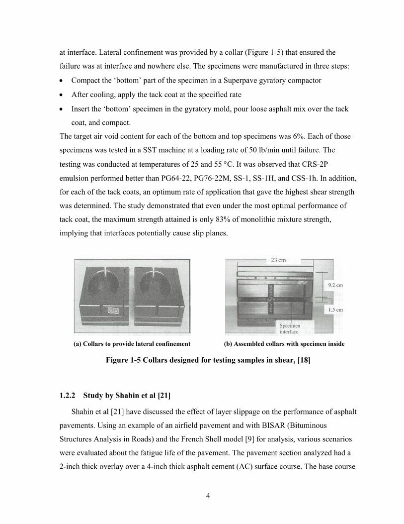
4
at interface. Lateral confinement was provided by a collar (Figure 1-5) that ensured the
failure was at interface and nowhere else. The specimens were manufactured in three steps:
• Compact the ‘bottom’ part of the specimen in a Superpave gyratory compactor
• After cooling, apply the tack coat at the specified rate
• Insert the ‘bottom’ specimen in the gyratory mold, pour loose asphalt mix over the tack
coat, and compact.
The target air void content for each of the bottom and top specimens was 6%. Each of those
specimens was tested in a SST machine at a loading rate of 50 lb/min until failure. The
testing was conducted at temperatures of 25 and 55 °C. It was observed that CRS-2P
emulsion performed better than PG64-22, PG76-22M, SS-1, SS-1H, and CSS-1h. In addition,
for each of the tack coats, an optimum rate of application that gave the highest shear strength
was determined. The study demonstrated that even under the most optimal performance of
tack coat, the maximum strength attained is only 83% of monolithic mixture strength,
implying that interfaces potentially cause slip planes.
(a) Collars to provide lateral confinement
(b) Assembled collars with specimen inside
Figure 1-5 Collars designed for testing samples in shear, [18]
1.2.2 Study by Shahin et al [21]
Shahin et al [21] have discussed the effect of layer slippage on the performance of asphalt
pavements. Using an example of an airfield pavement and with BISAR (Bituminous
Structures Analysis in Roads) and the French Shell model [9] for analysis, various scenarios
were evaluated about the fatigue life of the pavement. The pavement section analyzed had a
2-inch thick overlay over a 4-inch thick asphalt cement (AC) surface course. The base course

5
was 25-inch thick with elastic modulus of 75000 psi and a CBR value of 80. The subgrade
was very weak with California Bearing Ratio (CBR) of 5 and stiffness of 7500 psi. The
tensile stress at the bottom of the asphalt layers (overlay and the original surface course) and
the vertical compressive strain on the subgrade were the criteria for failure. It was found that
for full friction between the interfaces, the maximum tensile strain in the section is located at
the bottom surface of the original asphalt layer. If the slippage was allowed below the
uppermost layer, the tensile strain also existed at the bottom of the overlay. In addition, the
following observations were made:
• Only a small amount of slippage is sufficient to produce strains in the pavement that
approach those of the free slippage case.
• The tensile stress at the bottom of the overlay causes a compressive stress to develop on
the upper surface of the asphalt surface layer. This causes a relative movement of points
on the either side of the interface. This distortion further weakens the bond between the
asphalt layers, allowing more slippage leading to higher strains.
• The subgrade strains increase with increasing slippage. Because two thinner layers are
not as stiff as a single layer of the same overall thickness, the compressive vertical strain
on the subgrade increases.
• Further, under the action of horizontal loads, the study found that for no friction, the
horizontal strains are much higher than those with full friction.
The principal normal tensile strains, developed by the horizontal loads along the back edge of
the contact area, are of the same magnitude and cause progressive failure along the rear edge.
This tensile failure would cause slippage cracks in the overlay. If the overlay is not properly
bonded to the underlying layers, the overlay moves resulting in opening of the cracks. These
cracks are crescent shaped. In order to fix these cracks, either the existing layer needs to be
removed and re-paved or a thicker well-bonded overlay be placed on the existing overlay. In
addition to strong interlayer bonding, the authors suggested an overlay stiffness of at least
500,000 psi.
1.2.3 Study by Uzan et al [30, 31]
A research to evaluate the adhesion between asphalt mixes was conducted by Uzan, et
al. [30, 31] using the Goodman’s constitutive law:

6
τ = K × ∆u (Equation 1-1)
where:
τ is the shear stress at interface,
∆u the relative horizontal displacement of the two faces at the interface, and
K is the horizontal interface reaction modulus.
The interface behavior was described, which formerly was restricted only to perfectly rough
or perfectly smooth conditions. The analysis was carried out using the BISAR program for a
test section at different levels of adhesion. It was observed that for a perfectly smooth
interface (K=0) the tensile radial strain at the bottom of the uppermost layer was higher than
for the perfectly rough interface. The top of the second layer also changed to compressive
strain when K approached zero. Further, it has been shown that even an adherence of 90%
was very close to a smooth condition as described in Shahin et al [21]. Direct shear tests were
performed on the layered asphalt concrete specimens with shearing along the tack coat and
the variables were temperature, vertical pressure and rate of application of tack coat (Figure
1-6). It was concluded that the components of the interface shear strength were:
• Adhesion, represented by the tensile properties of the slip plane.
• Interlocking, from the penetration of aggregates into the voids of the other layer. The
interlocking component depends on the texture of the surfaces in contact and properties
of the asphalt mix.
• Friction, from rugosity of the two faces. Further, the friction component was included in
the other two components. It was suggested that measurement of the adhesion
component, which is indicated by rupture of the bond between layers in the bitumen or
mastic phase, could be done by a tensile test. (The interlocking effect would be absent for
pure tension.)
The following factors largely influenced the interface shear strength:
• Temperature: It is known that temperature affects the asphalt properties. The stiffness
decreases with increase in the temperature and vice versa. The effect of higher
temperatures is more dominant while testing in tension than in compression. In order to
offset the effect of increased temperature, higher vertical pressures are applied. With

7
increasing vertical pressures, the interlocking component gets more dominant than the
adhesion component.
• Tack Coat Rate: The tack coat bonding the two layers usually functions in two ways:
(a) Fill voids on the surface.
(b) Increase the interface film thickness or get absorbed in the adjacent layers.
The filling of voids on the surface of the mixes increases the contact area and
consequently the adhesion. However, excessive film thickness decreases the adhesion
and aggregate interlock. Very low tack coat rate could mean loss of adhesion
component. Hence, it is required that the tack coat be applied at optimum rate.
• Rate of Deformation: The rate of shear deformation is an important factor in controlling
the strength and deformation ability of the interface. Generally, with increasing rate of
deformation, the magnitude of stress developed increases.
Shear Force
Figure 1-6 Schematic of specimen deformation during shear testing, [31]
1.2.4 Study by Tschegg et al [29]
A common method for measuring the bond strength of asphalt cores is the pull-off
test [29]. For this test, cores with a diameter of 100 mm were drilled from the top surface

8
down through the overlay, through the interface, and about 50 mm into the base layer. Steel
plates were glued to the top surface of the cores. Then the drill core was pulled off with a
tension machine in axial direction of the base layer. The maximum load is registered during
the pull-off test. This is a simple test method but gave only the adhesive tensile strength and
showed extensive scattering of results. The reasons for wide scattering of results were:
eccentricity of load, small core diameter and large aggregate size, notches at the surface of
the cores by drilling or burst out aggregates, stress concentrations, uncontrolled temperature,
and indentation effects owing to rough surfaces. In addition, the test was useless if the tensile
strength of the mix was lower than the interface bond strength.
For avoiding such drawbacks, a ‘Wedge Splitting Test’ was developed. In this test, a
block of asphalt concrete was made to crack along a predetermined joint at steady rate. The
splitting was done by a wedge that was located in a groove between the two blocks of
asphalt. The force and the displacements were recorded during stable crack propagation until
complete separation of the specimen took place. Based on the shape of the force-
displacement curve, a differentiation between brittle and ductile behavior is possible. Figure
1-7 and Figure 1-8 show the test setup and the specimens used for testing purposes. It was
found that with increasing temperature, the plastic behavior of the asphalt increased. There
was a decrease in the peak load values with an increase in the temperature. At low
temperatures, it was found that the relationship between the force and the crack opening
displacement was linear. However, this test could not distinguish between the two different
types of tack coats used for that study.
1.2.5 Study by Ameri-Gaznon et al [6]
Ameri-Gaznon et al [6] evaluated the octahedral shear stress (OSS) and the octahedral
shear stress ratio (OSR) for different pavement sections. In particular, the OSR and the rut
resistance in an asphalt concrete pavement (ACP) overlay is evaluated based on the overlay
thickness, interlayer bonding, effect of stiffness, and horizontal surface shear. The material
properties of the bituminous materials were evaluated using the tri-axial test and cohesion, c,
and angle of internal friction, φ, values were determined at 104 °F at a loading rate of 4-inch
per minute. The modified ILLIPAVE finite element computer program was used to calculate
the OSRs within ACP layers.

9
Figure 1-7 Specimen shapes for wedge splitting tests, [29]
Figure 1-8 Setup of wedge splitting test, [29]
In absence of interlayer bond, the overlay acts independently of the rest of the
pavement system allowing greater relative movement in between two asphalt layers. This
reduces the confining stress causing larger OSS in the overlay. Pavements of various

10
thicknesses have been analyzed and the 4-inch thick overlay is the most critical one when
there is free slippage.
With increase in the bonding, the critical thickness increases to 6 inches for ACP
overlays. For a complete bond, the stress levels are critical at the mid height of the ACP
overlay. With loss of bond, the critical stress shifts to the bottom of the surface layer. Also,
the stress levels are far more critical than when a complete bond exists. Typically, with
increasing stiffness, it is expected that the shear stresses would decrease but it works
otherwise if there is a poor interlayer bond. The authors have also considered the effect of
horizontal surface shear on pavements. It has been shown that presence of horizontal surface
shear force doubles the OSS induced in the ACP overlay for full bond and no-bond
conditions.
1.2.6 Study by Ishai et al [15]
The authors have carried out an investigation on the functional and structural role of
prime coat in flexible pavements. The areas of investigation were the contribution of prime
coat to pavement performance and evaluation of emulsions as an alternative source of prime
coats. The experimental program consisted of following:
• Evaluation of the rate of increase of viscosity and evaporation characteristics of the prime
coat material;
• Measurement of absorption of prime coat material into the base course;
• Quantification of change in the hardness of the base layer with time;
• And adhesion between the base course and the asphalt layer;
The conclusions drawn from the tests were:
1. Cutbacks had higher viscosity than the emulsions. Hence, it was necessary to heat the
cutbacks whereas there was no such problem with emulsions.
2. Rate of loss of liquid for emulsions is much higher than for cutbacks. This translates into
faster construction of the overlying pavement structure. Also retention of organic vapors
from cutbacks in the base layers could be detrimental to the overlying ACP, if paved
immediately. In addition to this, cutback residues have lower viscosity than the emulsion
residue, which translates to poorer interlayer bond for cutbacks.

11
3. The penetration of cutback was higher than that of the emulsions for granular material but
for sandy material the values were comparable.
4. The surface hardness of the base layer was measured using a pocket penetrometer. It was
found that for cutbacks there was not a significant gain of strength in the first ten days of
curing, however, for emulsions, the strength gain was much faster. The accelerated rate
of strength gain can be attributed to harder asphalt in the emulsions and faster curing.
5. The interfacial adhesion was measured using the direct shear test performed on composite
samples of base and asphalt concrete layers. For unprimed surfaces, the failure was
observed along the geometric interface between two layers. For a cutback prime coat, a
little bonding was observed due to the interlocking effect created by absorption of the
asphalt. The highest interface adhesion was observed when priming was done with
emulsions. This could be because of deep penetration and strong adhesive bonds. Also,
the failure shear stress was observed to be dependent on the vertical load due to more
efficient interlocking and greater adhesion.
It can, therefore, be concluded that emulsion based prime coats enhance the shear strength of
the interface at base and asphalt concrete layers.
1.2.7 Study by Hachiya et al [12]
The study consisted of mainly three steps. The first step consisted of analyzing the
airport runway and taxiway using BISAR to calculate the interface shear stresses and strains.
The results showed that shear stresses at interfaces depended on surface layer thickness
(lower thickness producing higher shear stresses) and horizontal force on the surface. An
increase in the horizontal force, in form of acceleration and braking, caused an increase in the
interfacial shear stresses. The pavement failure was caused by interlayer separation due to
increased shear and tensile cracking at the bottom of the top layer. Construction of thicker
lifts can help reduce the interlayer shear stresses. In the second step, laboratory tests were
conducted on asphalt concrete specimens (Figure 1-9) and emulsions (Figure 1-10) in the
laboratory. Asphalt specimens were tested in shear and tension at various temperatures in a
strain-controlled mode. The interfaces (Figure 1-9) were hot jointed, cold jointed, tack coated
(0.088 gal/yd2) and monolithic. Tack coated joints performed better than cold joints but not

12
as well as hot joints or monolithic construction. The interlayer shear strength was dependent
on type of tack coat used (modified emulsions worked best), rate of application, curing time,
and temperature. In the third part, three sections were constructed and subjected to loading by
an assembly similar to aircraft landing gear. The top layer in each of the sections was of the
same thickness but constructed differently: for the first section it was constructed in three
lifts, for the second it was in two lift, and for the third it was a single lift. It was observed that
the section constructed in a single lift rutted more than the other two. The section least likely
to rut was the one with three lifts. Overall, it was suggested to use higher lift thicknesses and
modified emulsions to reduce the interlayer slippage on airport pavements.
Figure 1-9 Specimen shapes and testing method, [12]
Figure 1-10 Shear test on emulsions, [12]

13
1.2.8 Study by Mukhtar et al [19]
Tests similar to the current study were conducted by Mukhtar et al [19] to evaluate
the shear strength of AC-PCC interface. PCC specimens of dimensions shown in Figure 1-11
were cast and cured for a period of 28 days. Subsequently, a tack coat was applied at one of
the surfaces and the PCC specimen was inserted in the mold having 2-inch internal diameter.
Loose asphalt mix was compacted to a density of 147 pcf in three lifts each with 1-inch
thickness. A vertical confining load of 79 psi was applied to simulate the field condition of
having a 2.5-inch thick AC overlay over PCC. The specimens were then sheared at interface
in a strain-controlled mode at the rate of 1.0, 30 and 300 inch per min. The testing was
carried out at of 0, 20, 40, 60, 80 and 100 °F. It was observed that, regardless of the testing
temperature and shearing rate, monolithic AC specimens had higher shear strength than
specimens jointed at the interface. The shear strength of the interface increased with higher
rate of shear and lowering of temperature. Analysis performed by the authors indicated
maximum shear stresses below the wheel.
Figure 1-11 Specimens with tack coat at interface, [19]
1.2.9 Study by Sholar et al [24]
The authors have investigated the effect of different tack coat application rates, curing
time, types of aggregates, rates of shear and moisture on the interfacial bond strength of
composite asphalt specimens. A device, shown in Figure 1-12, was developed to test the

14
specimens in shear. The device was mounted in a temperature controlled MTS test chamber.
The shear strengths of composite samples were measured at constant strain rates. The shear
strength of the interface was directly related to the rate of shear and inversely to the test
temperature. It was observed that exposure of tack coat to moisture, prior to paving a new
overlay, caused reduction in the interfacial shear strength. This emphasizes the need to have
proper curing of tack coats before paving a new layer. Further, coarser gradations (19.0 mm)
performed significantly better than finer (12.5 mm) gradations in terms of shear strengths. In
addition, milling of the existing pavement surface before applying tack coat significantly
increased the bond strength of the interface in shear. Increasing the rate of application of tack
coat caused a marginal increase in the shear strength of the interface.
Figure 1-12 Shearing device developed by Sholar et al [24]
1.2.10 Prime Coats
Prime coating is the spray application of asphalt on the surface of a non-asphalt base
course. Usually untreated materials are primed with cutback asphalt that helps waterproof the
surface of the base, plug capillary voids, coats and bound loose mineral particles, and provide
adhesion between the base and asphalt concrete. Although, emulsion based primes have been
used as an alternative to cutback, HMA industry experience suggests that emulsions are not
15
as effective as cutbacks. Due to this reason, for many asphalt pavement constructions,
priming is completely eliminated.
Asphalt Institute suggests that prime coats be used for asphalt layers less than 3-4
inches thick. This issue is particularly important for thick pavements placed directly on sub-
base or base materials, especially in case of low-volume roads. During construction of
pavement sections, asphalt concrete mats are usually placed in 1.5-2 inch lift thicknesses.
Construction equipment such as rollers and heavy truck traffic can induce slippage distress in
the first AC layer placed over the base even before the pavement is open to traffic. It is,
therefore, critical to understand the contribution of prime coat in dissipating the induced
shear stresses. Prior studies on the subject of prime coats have investigated the effectiveness
of emulsions versus cutbacks, effectiveness of different emulsions, and construction
techniques to improve prime coat performance. The current study measures the interlayer
bond strength for various prime coats and attempts to correlate them to the mobilized
interlayer shear stresses in typical pavement sections.
1.2.11 Tack Coats
In composite asphalt concrete pavements, tack coat provides the interface bond
between two AC layers or between AC-PCC layers so that they form a monolithic structure
to withstand traffic and environment. A strong tack coat is essential to dissipate the shear
stress within the pavement structure. Factors such as traffic level, interface bond strength and
surface-layer thickness directly affect the performance and life of the pavement. The study
outlined in the next section compares the bond strength of field cores tacked with PG64-22
and CRS-2.5. Certain types of tack coat (e.g. PG 64-22) have been found to perform better
than others (e.g. CRS-2.5 emulsion). The efficient use of tack coat is critical for asphalt
overlay construction, especially for overlay of the rigid concrete pavement surfaces that need
to be opened to traffic within 12 to 24 hours. In many cases contractors preferably use PG64-
22 asphalt cement as a tack coat over CRS-2.5 emulsion because the former does not require
any curing before traffic can be applied.
For overlay as well as new construction of AC pavements, asphalt concrete mats are
usually placed in 1.5-2 inch lift thicknesses. As discussed earlier for prime coats,

16
construction equipment and heavy truck traffic can induce slippage distresses during
construction that can propagate to the surface. It is, therefore, necessary, to understand the
relationship between tack coat bond strength and pavement layer thickness for dissipation of
traffic induced shear stresses.
1.3 Research Need
The extensive network of highways and interstates add up to very high maintenance
costs. The delamination distresses are due to traffic acceleration and deceleration. Poor tack
coat undermines the pavement condition at these locations by increasing the shear stresses
significantly. A study, that evaluates the material properties as well as their suitability, would
enhance the quality of ride and extend the life of pavements thereby reducing the associated
direct and indirect costs.
1.3.1 Prior Work
The motivation for this study was from an investigation launched in Division 13 of
North Carolina Department of Transportation (NCDOT), by Tayebali et al [28] to examine
the severe distresses manifested in the form of asphalt concrete layer delamination and
distortion. The goal was to evaluate and identify the causes of delamination and distortion of
asphalt concrete mat. The methodology adopted for investigation consisted of evaluating the
field cores and testing of laboratory prepared specimens. In the first stage a survey was
conducted across plants in Division 13 of NCDOT to acquire information about the use of
different tack coats and type of material used in the field. Based on the questionnaire
responses, two sections were chosen, each with a different type of tack coat. Enka,
Buncombe County and Rutherfordton, Rutherford County had CRS-2.5 emulsion and PG64-
22 binder, respectively used as a tack coat.
After the selecting the section, cores of 4-inch and 6-inch diameter were drilled from
distressed and non-distressed areas from two counties. The 4-inch specimens were used to
determine whether the mixes confirmed to the NCDOT job mix formula specifications based
on air voids and Marshall mix design criteria. It was found that the mixes indeed confirmed
with the NCDOT specifications and the only possible cause of distress could be improper

17
interlayer bonding or construction technique. An on-site inspection and initial survey
indicated no such construction abnormalities and the focus was to evaluate the interlayer
bonding. The 6-inch diameter cores were tested on the Simple Shear Test (SST) machine.
A frequency sweep test at constant height (FSCH) was conducted on the cores from
distressed and non-distressed sections. The test measures the shear viscoelastic properties
(dynamic shear modulus, |G*|, and the phase shift, δ) over a range of testing frequencies and
at different temperatures. It should be noted that the measured dynamic response of the core
is a composite response of the two asphalt layers separated by a thin film of tack coat. It was
concluded from the FSCH test that cores from non-distressed sections had higher |G*| and
G*/sin δ values over the cores from distressed sections. This implied that the non-distressed
mixes had a higher stiffness and a lower propensity to rut justifying their better performance.
The repeated shear test at constant height (RSCH) was used to measure the rutting
potential of the mix over a range of temperatures. This test is performed in a controlled stress
mode in accordance with AASHTO TP-7, Procedure F [5]. The RSCH gave results similar to
FSCH. It was found that non-distressed cores withstood higher number of cycles than the
distressed cores. Also, for cores from Buncombe County (CRS-2.5) there was a distinct
difference between the ‘good’ and ‘bad’ (i.e., non-distressed and distressed) cores.
Examination of the failed core samples showed a distinct pattern of cracking with diagonal
cracks in both upper and lower asphalt concrete layers with a horizontal crack joining the
diagonal cracks at interface. It should be noted that CRS-2.5 was used as a bonding (tacking)
agent. For Rutherford County (where PG64-22 binder was used as tack coat) the difference
in the number of cycles to failure was relatively smaller and the failure pattern was consistent
with that observed in a monolithic single layer specimen. In addition to this, no interlayer
separation or horizontal crack was evident at the interface. It should be noted that Rutherford
County cores used PG64-22 as a tack coat. Thus, it was shown that the type of tack coat
contributes significantly to the performance and the interface failure pattern.
An axial frequency sweep test (AFST), similar to the FSCH, was performed on the 6-
inch diameter specimens. A dynamic axial load is applied and the dynamic axial stiffness
modulus (|E*|) along with the phase shift, δ, of an asphalt mix are measured. Ideally, taller
specimens would have been preferable but the test was conducted on samples of 50-mm
height. The trend in |E*| values was very much similar to that of |G*| for both the counties

18
and |E*| was found to be higher for non-distressed specimens. Thus, the results were found in
agreement with the FSCH and it also proved that this test was robust to detect the difference
between ‘good’ and ‘bad’ cores. In the ramp test, the specimens were pulled apart at a rate of
2.5-mm/minute after gluing them to metal platens. This test was used to measure the tensile
strength of asphalt mixtures and, in particular, for layered specimens it represented the
(tensile) strength of the interfacial joint. It was found that bond strength of the CRS-2.5
emulsion was 46% lower compared to cores from Rutherford County. The failure of
Rutherford County cores was in the mix whereas for the Buncombe County cores, the failure
was at the interface. Based on the field core test results, it was concluded that sections tacked
using PG64-22 binder performed better when compared to sections tacked with CRS-2.5
emulsion. However, it may be noted that based on field core test results it was not possible to
conclude whether PG64-22 was a better tacking material than CRS-2.5. This was because the
rate of tack coat application could have been different and/or a construction problem such as
uniform application, emulsion curing time before construction, and environmental issues.
Therefore it became imperative to investigate, in a controlled laboratory test program,
whether PG64-22 was indeed superior to the use of emulsions as a tacking material.

19
2 Research Approach and Methodology
2.1 Objective
The goal of this investigation was to mechanistically evaluate the contribution of
prime and tack coat in composite asphalt concrete pavements. The current work
undertaken for this study was based on the work conducted earlier [28]. In order to
comprehend the contribution of prime and tack coats, it was necessary to understand and
quantify the distribution of interlayer shear stresses, and their effect on the interface
bonding. The project has two main components: experimental and analytical. The
experimental part involves determination of material properties; and the analytical
portion involves mechanistic analysis using the developed software that will enable the
selection of appropriate pavement thickness and/or the choice of tack coat given an input
of material properties, structural thicknesses and loading conditions. The result of this
study will also enable designers to choose appropriate tacking materials for specific
application. At the same time, with regard to prime coats, the use of emulsions has not
been very popular in comparison to cutbacks. Specifically, many highway agencies (AZ,
KS, NE, NH, NY and RI) do not use prime coats (emulsion based) any more.
2.2 Research Methodology
In order to achieve the objectives stated above, this investigation was conducted using
the following tasks described below and as shown in Figure 2-1.
2.2.1 Literature Review and Survey
In this task, a review (§1.2) on the contribution of prime and tack coats to pavement
performance was conducted. A survey questionnaire (Appendix A) was designed and sent
to all state highway agencies to gather data on their experience for pavement construction
with and without the use of prime and tack coats.

20
2.2.2 Asphalt and Mastics Testing
The Asphalt Institute Manual Series MS-16 [7] recognizes the detrimental effect of
rounded particles and its contribution to mixture instability. Although the present mix in
NCDOT Division 13 may not contain high sand content, it was hypothesized that the
variable amount of baghouse fines purged intermittently into the asphalt mixture may
account for the mix instability and significant changes in volumetric properties.
Therefore, the objective of this (§2.2.2) and the next task (§2.2.3) was to evaluate
contribution of baghouse fines. The objective of this task was to evaluate the rheological
properties of the binder in presence of baghouse fines using a Dynamic Shear Rheometer
(DSR). This task consists of three subtasks:
• evaluate the properties of aged and virgin binders,
• rheological properties of mastics (aged and unaged), and
• viscosity of virgin asphalts and emulsion residues using rotational viscometer.
2.2.3 SST Testing of SGC Specimens, TSR and APA Tests
The objective of this subtask was to evaluate the effect of baghouse fines on mix
characteristics using controlled mixes, and investigate their sensitivity to moisture
exposure. Raw materials including baghouse fines and job-mix were obtained from
NCDOT Division 13. Two mixes were prepared in the laboratory based on the job mix
formula with materials passing #200 sieve (mineral filler) containing:
• zero percent baghouse fines; and
• 100 percent baghouse fines.
All other mix parameters such as asphalt content, and aggregate gradation were kept
constant. These two mixes were subjected to the following laboratory testing:
• Laboratory FSCH and RSCH test on 6-inch diameter specimens compacted using
SGC;
• Georgia wheel rutting test at NCDOT M&T Unit on 6-inch diameter specimens
prepared using SGC; and
• Moisture sensitivity testing using the modified AASHTO T283 procedure.
21
2.2.4 Material Characterization
The objective of this task was to obtain material characteristics that would be needed
for mechanistic analysis of the pavement sections elaborated in Chapter 9. The
compressive strength and the elastic modulus of the PCC specimens were evaluated using
cylindrical specimens. The CTB properties were also determined in the lab. For the
asphalt concrete mix, the axial and shear stiffness were characterized at different
temperatures and frequencies. Stiffness versus frequency master curves were prepared
from the data obtained. These results would enable the selection of the appropriate
stiffness and moduli values required for the mechanistic evaluation.
2.2.5 Fabrication of Slabs and Test Specimens
In this task, composite specimens – AC over AC, AC over PCC and AC over CTB –
were fabricated using rolling wheel compaction. Approximate size of the slab was 24-
inches by 24-inches. To cast the slabs, steel molds were fabricated. The lower layer of the
slab was either be 2-inch thick CTB layer or PCC layer for the evaluation of prime and
tack coats, respectively. The CTB and PCC layers were allowed to cure for 7-days.
Appropriate prime and tack coat was applied (to CTB and PCC, respectively) and
allowed to cure according to manufacturer’s recommendation.
For prime coat evaluation, slabs were prepared without any prime coating, and using
three prime coats that are on NCDOT’s approved product list. These were EPR-1, CSS-
1h and EA-P. Similarly for tack coat evaluation, slabs were prepared without any tack
coating, and using a CMS-2 emulsions and PG64-22 asphalt cement. A dense mix asphalt
concrete layer was then be rolled using a rolling wheel compactor. After the mix cooled
down, the slabs were cored to produce 6-inch diameter specimens, which were tested in
shear for bond strength properties.
2.2.6 Bond Strength Determination using Shear Testing
The objective of this task was to evaluate the CTB-AC, AC-AC and PCC-AC layer
interface bond strength for various prime and tack coats used. In this study, the bond

22
strength was proposed to be evaluated using the simple shear test at constant height.
Testing was conducted at 40 and 60 °C. For AC-AC and PCC-AC interfaces the testing
was conducted at 20 °C as well. Two different shear strain rates were applied. Two
replicates were tested at each strain level. For a given shear strain rate, the shear and axial
stresses were monitored and the bond strength determined for each prime and tack coat
being evaluated. In addition to the testing of composite core specimens, an attempt was
also made to test prime and tack coat using two metal platens.
2.2.7 Mechanistic Analysis
Three dimensional stress analysis software based on semi-analytic method was
developed as part of the overall project. The pavement was modeled primarily as a
layered system of linear elastic materials with surface asphalt layer as a elastic material.
Using the software, a detailed parametric study was conducted to investigate the effect of
system parameters including layer thickness and stiffness on the stress-strain-
displacement fields induced in the pavement. The effect of vehicle load characteristics on
the response was also examined.
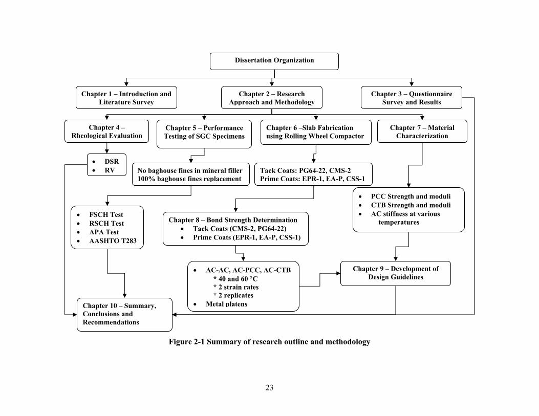
23
Figure 2-1 Summary of research outline and methodology
Chapter 4 – Rheological Evaluation
Dissertation Organization
Chapter 9 – Development of Design Guidelines
Chapter 1 – Introduction and Literature Survey
Chapter 2 – Research Approach and Methodology
Chapter 3 – Questionnaire Survey and Results
Chapter 7 – Material Characterization
Chapter 5 – Performance Testing of SGC Specimens
Chapter 6 –Slab Fabrication using Rolling Wheel Compactor
Chapter 8 – Bond Strength Determination • Tack Coats (CMS-2, PG64-22) • Prime Coats (EPR-1, EA-P, CSS-1)
Chapter 10 – Summary, Conclusions and Recommendations
• PCC Strength and moduli • CTB Strength and moduli • AC stiffness at various
temperatures
Tack Coats: PG64-22, CMS-2 Prime Coats: EPR-1, EA-P, CSS-1
• AC-AC, AC-PCC, AC-CTB * 40 and 60 °C * 2 strain rates * 2 replicates
• Metal platens
• DSR • RV No baghouse fines in mineral filler
100% baghouse fines replacement
• FSCH Test • RSCH Test • APA Test • AASHTO T283

24
3 Survey Results
3.1 Development of Questionnaire
The goal of the current investigation was to examine the effect of various tack and prime
coats on interface strength. In order to acquire the information regarding the use of different
tack coats and prime coats in the field, it was necessary to conduct a survey of highway
agencies. The expected outcome from the survey was to identify overall trends in prime and
tack coating, and evaluate the scope for potential improvement.
The developed questionnaire (Appendix A) was sent to various state highway
departments and agencies for their responses. Information collected was:
• whether prime coat was required for new construction,
• rate of its application,
• relation of prime coat to asphalt pavement thickness,
• curing time,
• laboratory tests for prime coats,
• field performance tests
• difference between pavements with and without prime coats,
• merits of emulsified asphalts versus cutback asphalts
• types of materials used for tack coats and their application rates, and
• provisions for emulsion breaking under nighttime paving conditions.
3.2 Survey Responses
In all more than 50 questionnaires were sent out and 26 replies have been received to
date. The responses of the survey are summarized in Appendix B, and the observations are
summarized below:
1. The following states responded to the questionnaire: Alabama, Alaska, Arkansas,
Arizona, Connecticut, Florida, Georgia, Idaho, Illinois, Kansas, Kentucky, Maine,
Minnesota, Mississippi, Missouri, Nebraska, New Hampshire, New Jersey, New York,

25
Oklahoma, Rhode Island, South Carolina, Tennessee, Texas, West Virginia, and
Wyoming.
2. Ten of the 26 states reported that there is no requirement of prime coat for new
construction of the pavement. Two highway agencies Oklahoma and Alaska leave it to
the individual designers and mention that it depends on the location in the state.
3. Of the remaining sixteen states using prime coats, seven (AL, AR, NJ, WY, OK, and IL)
reported using only cutbacks for prime coat as opposed to emulsions. For the remaining
nine states, most of them used a combination of emulsions (diluted or undiluted) and
cutbacks; there were states that preferred only emulsions, e.g. WV, CT, KY and TN.
4. For prime coats,
(a) Cutbacks that are currently used in practice are: MC-30, MC-70, MC-250, RC-30,
RC-70, and RC-250; and
(b) The emulsions used are: AE-90, AE-150, AE-200, AE-P, CAE-P, CMS-2h, CSS-1,
CSS-1h, EA-1, EAP-1, EAP&T, EP, EPR-1, MS-2h, PCE, SS-1, SS-1h and Primer-L.
5. In most of the cases, it was reported that cutbacks penetrated better than emulsions. The
coverage offered by cutbacks was greater than emulsions. However, there were states that
have noted the following in preference to emulsion over cutbacks as prime coats:
• MS (emulsions, when applied properly, are easier to work with),
• MO (emulsions have more pickup versus cutback),
• IL (emulsions for resurfacing projects) and
• TX (emulsions good for open bases)
The cutbacks did not have any curing problems and hence were preferred where it was
not possible to wait for the emulsions to break.
6. The rates of application of the prime coat range from 0.03 to 3.44 gal/yd2. In some cases,
emulsions were diluted before applying thus reducing the concentration of the emulsion
e.g. Florida. The rates of application depended on the type of base, as was the case with
Mississippi and Alabama. For Maine, the rate was 0.02 gal/yd2 for overlays, 0.04 gal/yd2
for milled, and 0.01 gal/yd2 for new mixes.
7. No specific basis was reported for the curing time of prime coats. In most of the cases,
the states did not consider curing time. For those states that required curing, the criteria
were subjective such as “tacky to touch” or duration ranging from 1 hour to 3 days. For
26
Oklahoma the condition was stated as “sufficient to allow proper penetration and
hardening of prime coat,” which is quite difficult to assess without testing. Texas requires
that the emulsions be worked into the top one inch of the layer and the layer re-
compacted.
8. The thickness of the pavement layer has relatively no relevance to the required use of
prime coat. Georgia and New Jersey require it if the AC thickness is 125-mm (5-inch) or
less whereas the limit for Missouri is 100-mm (4-inch). Illinois requires prime coat only
for full depth pavements. In spite of variation in the prime coat requirement, all agencies
require it where either the thickness is too low or there are lot of horizontal shearing
forces on the surface or where interlayer bond failure is likely to occur.
9. The laboratory tests needed to be performed on the emulsions and cutbacks are the
viscosity tests (kinematic), distillation, solubility in trichloroethylene, residue test and
float test. Most of the agencies do not have any field performance testing procedures or
requirements.
10. While most of the agencies admitted that prime coat does improve performance, there
were quite a few (50%) who did not see any difference in performance. Some of the
reasons cited for better performance were:
(a) Water proofing and creating an impervious barrier to moisture.
(b) Erosion control of the base.
(c) Reduction in shearing and tearing of thinner pavements – less than 2-inch thick - on
curves and on grades (Idaho). Less delamination and inability to separate the layers
without a saw. In Oklahoma, absence of prime coat had lead to significant plane
slippage problems.
(d) Ease of densification of SUPERPAVE™ mixes (New Jersey).
(e) Maintenance of optimal moisture content levels in the base thus maintaining the base
strength at a constant level.
11. The materials used as tack coat are: AC, AE-60, CMS-1, C-70, C-250, C-800, CMS-2,
CRS-1, CRS-2, CRS-2h, CSS-1, CSS-1h, HFE-60, HFE-90, HFMS-1, HFMS-2, HFMS-
2h, HFMS-2s, MC-250, MC-800, MS-1, MS-2, MS-2h, PG58-22, PG64-22, PG67-22,
RC-70, RC-T, RS-1, RS-2, SS-1, and SS-1h. Thus, a larger variety of materials can be
27
used as tack coats than prime coats. To reduce the concentration of asphalt, the emulsions
used for tack coats were diluted with water before application.
12. Tack coats are applied at the rate of 0.03 - 0.2 gal/yd2. In cases, where there was dilution
with water, the effective rate of application is within the above range. In South Carolina,
the rate of application is based on residual asphalt.
13. Nighttime paving: Most states require that the emulsion should break before the
placement of new layer, there has been no concrete method to verify such condition. For
a few states, the verification of the breaking of emulsion is done based either on touch -
tacky touch - or by observation of the inspector. Some states (OK) disallow use of
emulsions after sunset whereas states like Alabama are eliminating the use of emulsions
because of difficulty in determining the state of the emulsion (broken or not).
In summary, more than 38% of the responding highway agencies do not require prime
coats to be used, and some agencies only use it for relatively thin pavement sections (less
than 4 to 5 inches). The current practice of using tack coat in the form of emulsion varies
widely depending on the highway agencies. Clearly, there is a vast possibility of error in
construction technique that may result in poor performance, especially for night time paving
operations. Some of these difficulties have been mitigated by various highway agencies by
substituting PG64-22 as a tacking agent over emulsion tack coats.

28
4 Rheological Evaluation
4.1 Introduction
One of the concerns with respect to asphalt mixtures in NCDOT Division 13 was with
regards to the variable amount of baghouse fines purged intermittently in the production of
the field mixtures. This chapter deals with:
• the evaluation of the gradation of baghouse fines using the state-of-the-art particle
analyzer at FHWA Turner Fairbank Highway Research Center;
• the influence of fines on the rheological properties of asphalt cement using mastics
was also evaluated using the DSR; and
• the properties of residual asphalts and emulsions
4.2 Selection of Fines
For this study, the mineral filler and baghouse fines with materials passing #200 sieve
were obtained from Buncombe and Rutherford counties. The fines selected for analysis were:
• Buncombe County:
• passing #200 sieve fraction from wet screenings
• baghouse fines
• Rutherford County
• Passing #200 sieve fraction from dry screenings
• 'fine' baghouse fines
• 'coarse' baghouse fines.
In all, five different types of fines were analyzed using the particle analyzer.

29
4.3 Gradation Analysis of Fines using FHWA Particle Analyzer
4.3.1 Method Description
The gradation analysis of mineral fillers was carried out at the Turner Fairbank
Highway Research Center, McLean, Virginia. The material was separated using a small
splitter, then further separated using a micro splitter, to obtain a representative sample. To
run the test, a small amount of material was mixed in a medium to create a suspension. For
baghouse fines, distilled water with 1-percent sodium hexametaphosphate was used.
The testing process consisted of taking a ‘blank’ measurement of the medium to
establish a baseline. The material was then slowly introduced and mixed with the medium
until an ‘optimum’ intensity was found. In order to prevent particle agglomeration, agitation
by cavitation was induced by a high intensity ultrasonic processor for 2 minutes. The particle
analyzer automatically converted different light intensity measurements into particle size
distribution. The average of three different samples was obtained and the results were found
to be consistent with each other. The results, however, necessarily need not match with the
sieve analysis. The main reason for this is the fact that the gradation obtained from the laser
particle analyzer is a volume gradation based on the projection of particles. The device
showed the differences that were otherwise difficult to capture.
4.3.2 Results and Discussion
In all two sets of analyses were performed within the duration of this study. Figure
4-1 and Figure 4-2 show the gradations of the mineral fillers and bag-house fines obtained
from the two counties. Figure 4-2 presents the particle analysis performed on the first set of
fines received before the entire set of materials was requested so that a decision could be
made about the further analysis to be performed. Figure 4-1 presents the particle size analysis
that was carried out on fines received in the latter batch of materials from which the samples
for laboratory testing were actually fabricated.
For Rutherford County, the ‘coarse’ baghouse fines appeared to be ‘sandy’ and hence
their size distribution was measured using a slightly more viscous medium. The two media
used for Rutherford County ‘coarse’ bag-house fines were distilled water (W) and 90-percent

30
distilled water plus 10-percent glycerin (G). In Figure 4-2, the particle analysis results using
the two different media are fairly different. However, both media show that this sample is the
coarsest.
Figure 4-1 and Figure 4-2 show that the ‘coarse’ baghouse fines from Rutherford
County is the coarsest material passing #200 sieve. Although it was anticipated that the
baghouse fines, in general, would be finer than the regular fines passing #200 sieve, the
particle size analysis indicated for both set of materials that the baghouse fines from both
counties had more or less similar particle size distribution as the regular fines. Table 4-1
shows the properties of the fines based on the second set of materials which was used for
mixture performance testing in this study. The mean particle size of regular fines from
Buncombe and Rutherford counties are both 30.5-µm. The baghouse fines from Buncombe
County has the mean particle size 40-µm and the Rutherford County ‘fine’ baghouse fines
has a mean particle size of 31-µm. The ‘coarse’ baghouse fines from Rutherford County have
a mean particle size of 88-µm, more than twice the mean size of any other regular or
baghouse fines.
The particle size analysis suggests that based on gradation, the mixture performance
should not be affected whether the mineral filler used is regular fines or from baghouses.
However, as the particle shape and/or perhaps the mineral content distribution may be
different for the baghouse fines, it may have different effect on the rheological behavior of
the asphalt cement and mixtures in general. This effect is investigated in the following
section where the performance of baghouse and regular fines are studied using asphalt-fines
mastics in an aged and unaged condition. In Chapter 5, this effect is also evaluated based on
the performance of the asphalt mixtures.
4.4 Analysis of Asphalt-Fines Mastics using DSR
The objective of this task was to evaluate the rheological properties of the binders and
mastics containing baghouse fines at intermediate to high temperatures. Testing was
conducted in accordance with AASHTO TP5-93 [4].

31
4.4.1 Specimen Preparation
The asphalt cement used for the preparation of mastics was a PG64-22 supplied by
NCDOT. Four mastics were prepared using the fines received from Buncombe and
Rutherford counties. The asphalt cements and each of the mastics were tested in an unaged
and aged condition with at least three replicates. The following asphalt and mastic
combinations were used:
• PG64-22 binder (virgin and RTFO-aged) for both counties
• Mastic (virgin and aged) from the baghouse fines. Only the ‘fine’ baghouse fines
was used from Rutherford County.
• Mastic (virgin and aged) from the regular mineral filler (fraction passing #200
sieve) from both counties.
The prepared mastic was a mixture of the filler/fines with asphalt from the corresponding
county. The proportion of asphalt was 50-percent by weight of the total mastic. For
preparation of mastics, the fines and the asphalt binder were pre-heated to a temperature of
160 °C. The fines were then added slowly to the heated binder with constant stirring until
uniform, consistent agglomerate free ‘batter’ was obtained.
The asphalt binders were aged in an RTFO oven, while the mastics were aged in an
air draft oven due to the higher consistency of the mastics. Due to high consistency of
mastics, problems were encountered in recovery from the RTFO bottles. The mastics,
therefore, were poured in a PAV dish and were kept in an oven for a period of 85 minutes at
163 °C for aging to simulate the RTFO aging effect. One problem encountered with handling
the mastics was segregation of fines. Hence while pouring into the molds; it was necessary to
stir vigorously so as to have a uniform consistency for the DSR specimens.
4.4.2 Test Parameters
The asphalt cement and mastics were evaluated at three temperatures – 58, 64, and 70
°C. For the asphalt binder, the DSR spindle diameter of 25-mm with 1-mm gap was used. As
the mastics were more viscous, a spindle diameter of 8-mm with 2-mm gap was used.

32
Testing at 10 rad/s frequency and at different strain levels (strain sweep) was
conducted to establish for each asphalt binder and mastic, the linear viscoelastic region in the
strain domain (defined by AASHTO TP5 to be a range of strain values where the test
measurement |G*| does not vary more than 95-percent of the |G*| estimated at zero strain).
Based on the strain sweep test, the strain level for unaged and aged binders selected was 12
and 10-percent, respectively. For the mastics, the strain levels selected were typically in the
range of 1 to 2-percent for both aged and unaged binders.
Frequency sweep tests were conducted on the asphalt binders and mastics at the
frequencies of 0.01, 0.05, 0.1, 0.15, 0.5, 1.0, 1.59, 5.0, 10.0 and 20.0 Hz. The measured
parameters from the test results were the dynamic shear modulus |G*| and phase angle δ.
These results were then used to generate master curves at 64°C for dynamic shear modulus
|G*| and |G*|/sinδ.
4.4.3 Test Results and Discussion
Figure 4-3 and Figure 4-4 show the dynamic shear modulus as function of reduced
frequency at 64 °C for Buncombe and Rutherford counties. The raw DSR testing data is
presented in Appendix E. These figures show that in general:
1) aging tends to increase the |G*| values for both the asphalt binder and the mastics
as compared to the unaged condition;
2) |G*| values for the mastics are much higher than the asphalt binder (this trend is
expected as the mastics contain 50-percent fines);
3) in case of Buncombe County, the mastic containing baghouse fines have higher
|G*| values over the range in frequency as compared to the mastic containing
regular mineral filler material;
4) in case of Rutherford County, the mastic containing baghouse fines show similar
|G*| values over the range in frequency as compared to the mastic containing
regular mineral filler material.

33
Figure 4-5 through Figure 4-8 show the Superpave rutting parameter, |G*|/sinδ, as function
of reduced frequency at 64°C. For Buncombe County, mastic containing baghouse fines
shows higher |G*|/sinδ values both in aged and unaged condition as compared to the mastic
containing regular fines. For Rutherford County, the mastic containing baghouse fines shows
higher |G*|/sinδ values in unaged condition but about similar values in aged condition
compared to the mastic containing regular fines.
In summary, therefore, it appears that Buncombe County baghouse fines show different
effect on aging of asphalt as compared to the Rutherford County baghouse fines.
4.5 DSR Testing of Emulsions
In order to evaluate the properties of the residual binders in the emulsions, DSR testing
was conducted. As emulsions contain a large amount of water, they were broken prior to
being tested in the DSR. The following two approaches were used to break the emulsions:
• Rolling Thin Film Oven:
The rolling thin film oven, commonly referred to as RTFO, is commonly used to simulate
the short term aging of asphalt in laboratory. Although the oven uses a temperature of
163 °C for testing purposes, the emulsions were broken in RTFO at lower temperature of
85 °C to prevent excessive aging of AC. At the end of the 85 minute test it was found that
there was substantial presence of moisture indicated by soft and fluid nature of residual
asphalt as well as by presence of typical brown coloration on the inner walls of the RTFO
bottles. In the second round, the RTFO temperatures were increased to 105 °C, however
there was not a significant improvement in the results.
• Open heating:
Due to non-conclusive outcome of the earlier approach, it was decided to break the
emulsions using the shallow, flat pressure aging vessel (PAV) pans. The heating
temperature was raised to 135 °C (to ensure complete evaporation of water component)
with constant stirring at regular intervals (roughly 15 minutes). The total heating period
was 85 minutes, same as the duration of the RTFO test. The temperature of 135 °C was
chosen because it is the highest temperature that asphalt can be subjected to without a
34
significant risk of aging. Most of the emulsions broke satisfactorily using this approach.
The emulsion EA-P, however, did not break because of its polymeric nature. This
emulsion, therefore, was heated to a temperature of 155 °C and it broke after extensive
heating for 2 hours.
The DSR testing was carried out on the residual binders at the following temperatures:
52, 58, 64 and 70 °C. Using a 25-mm diameter spindle and 1-mm thick specimens, the
testing was carried out at a frequency of 1.592 Hz. Two tests were performed: a stress sweep
test to determine the linear range of the binder and an oscillation test at 1.592 Hz.
4.5.1 Test Results and Discussion
The results are summarized in Figure 4-9 through Figure 4-11 and Table 4-2. The
following conclusions can be drawn:
1. It can be seen that with increase in temperature, there is a continuous fall in |G*|/sinδ
values. The results yield a straight line when plotted on a log-linear scale. All the curves
had an R2 value of one indicating a very good fit.
2. The CRS-1H is the hardest (stiffest) residual binder and the CMS-2 has the softest
residual binder of all. These results are as expected.
3. The testing of CRS-1H binder posed problems at a temperature of 52 °C because the
binder was too stiff. The deformation caused by the applied stresses was too small to be
accurately recorded by the DSR.
4. The residual binders of CRS-1H, EA-P and I.A.S. emulsions have a ‘reported’ high
temperature PG rating of PG70 but their actual PG ratings are PG73.7, PG74.7 and
PG70.7 respectively. Similarly, CRS-Koch has a ‘reported PG rating’ of PG64 but the
actual PG rating is PG65.1 and CMS-2 has a ‘reported PG rating’ of PG52 but the actual
PG rating is PG57.1. The DSR testing, therefore, provides a more accurate classification
of the emulsions. Thus, the emulsions can be listed in the following order (of decreasing
stiffness):
• CRS-1H
• EA-P
• I.A.S.
35
• CRS-Koch, and
• CMS-2.
5. The polymeric nature of the EA-P emulsion, combined with the high ‘actual PG grade’ of
residual binder, explains the stability of the emulsion at elevated temperatures.
6. Based on the DSR results, it can be hypothesized that the tacking strength of the
emulsions would be directly proportional to their respective PG temperatures.
4.6 Brookfield Viscosity
A rotational viscometer determines the flow characteristics of the asphalt binder and
its ability to be pumped and handled at the hot mix plant. Testing of binders was conducted
in accordance with ASTM D4402 (Standard Method for Viscosity Determinations of
Unfilled Asphalts using the Brookfield Thermosel Apparatus). It measures the amount of
torque required to maintain a constant speed of a cylindrical spindle immersed in liquid
binder at a given temperature. The number of replicates for Brookfield Viscometer testing
was three. The testing was carried out at two temperatures of 150 and 135 °C.
From Figure 4-12 through Figure 4-14, it can be seen that the EA-P emulsion exhibits
a rapid decrease in viscosity compared to other emulsions. Further, CRS-1 and CMS-2
emulsions have relatively similar consistency at 150 and 135 °C whereas for all other
emulsions under consideration, there is a rapid drop in viscosity with increase in temperature.
This could suggest that CRS-1 and CMS-2 are preferable compared to their counterparts.
This is further reinforced by the fact that their viscosities are relatively independent of the
spindle RPM. The CRS-1H and IAS emulsions have comparable values however, IAS seems
more temperature susceptible than CRS-1H. Based on the test results, the acceptability in the
order of preference is CMS-2, CRS-1, CRS-1H, IAS and EA-P.
4.7 Conclusions
It was originally hypothesized that the one of the contributory factor to the
delamination and shoving distress observed in Buncombe County was the intermittent
purging of the baghouse fines in the field asphalt mixes. Results of the gradation analysis
show that the baghouse fines have similar, or in some cases coarser, gradation as compared

36
to the regular mineral filler used in these respective counties. The dynamic mechanical
analysis of the mastics using the DSR suggests that inclusion of baghouse fines in asphalt
mixtures may not have any detrimental effect. On the contrary, for Buncombe County, the
inclusion of baghouse fines appears to enhance the rut resistance of the asphalt mixture as
will be shown to be the case in Chapter 5. However, the effect of moisture sensitivity on the
mixtures containing baghouse fines needs to be evaluated before any final conclusion can be
made.
Table 4-1 Properties of fines from particle size analysis (set 2) [13]
Particle Property
Buncombe Baghouses
Buncombe Passing #200
Rutherford 'Coarse' Fines
Rutherford 'Fine' Fines
Rutherford Passing #200
Fineness Modulus (F.M.) 5.72 5.40 7.10 5.43 5.31
Coefficient of Uniformity (CU) 10.20 7.60 4.00 9.11 8.67
Coefficient of Curvature (CC) 1.73 2.15 1.72 1.96 2.28
Skewness Indicator (σ1)
2.25 2.31 1.14 2.60 2.30
Skewness Indicator (σ2)
4.40 2.90 2.75 3.88 3.59
Mean Particle Size (µm) 40.0 30.5 88.0 31.0 30.5
Table 4-2 Temperatures for residual binders when |G*|/sinδ ≥ 1.0 kPa
Emulsion Temp. (°C) PG ratingCRS-1H 73.7 PG70
EA-P 74.7 PG70 IAS1 70.7 PG70
CRS-Koch 65.1 PG64 CMS-2 57.1 PG52
1 The testing was performed at four temperatures and the results were extrapolated to determine the appropriate 1-kPa temperature. Extra testing was not felt necessary because the results were almost a straight line when graphed.

37
0
10
20
30
40
50
60
70
80
90
100
1 10 100 1000Diameter, µm
Per
cent
pas
sing
BNC FinesRford 'Coarse' FinesBNC P#200Rford 'Fine' FinesRford P#200
Figure 4-1 Gradation analysis of fines using FHWA particle analyzer, set 2
0
10
20
30
40
50
60
70
80
90
100
1 10 100 1000Diameter, µm
Per
cent
pas
sing
BNC Bag FinesRford "Coarse" Bag (W)Rford "Coarse" Bag (G)Rford "Fine" BagRford Reg. Screen
Figure 4-2 Gradation analysis of fines using FHWA particle analyzer, set 1

38
1.E+00
1.E+01
1.E+02
1.E+03
1.E+04
1.E+05
1.E+06
0.001 0.01 0.1 1 10 100 1000Reduced Frequency, Hz
|G*|,
Pa
U. BinderA. BinderU. P200A. P200U. FinesA. Fines
Figure 4-3 Master curves (|G*|) for Buncombe County, 64 °C
1.E+00
1.E+01
1.E+02
1.E+03
1.E+04
1.E+05
1.E+06
0.001 0.01 0.1 1 10 100 1000
Reduced Frequency, Hz
|G*|,
Pa
U. BinderA. BinderU. P200A. P200U. FinesA. Fines
Figure 4-4 Master curves (|G*|) for Rutherford County, 64 °C

39
1.E-02
1.E-01
1.E+00
1.E+01
1.E+02
1.E+03
1.E+04
1.E+05
1.E+06
0.001 0.01 0.1 1 10 100Reduced Frequency, Hz
|G*|
/ sin
P
a
BinderBagfinesP#200
Figure 4-5 Master curves (|G*|/sin δ) for Buncombe County, unaged, 64 oC
1.E-02
1.E-01
1.E+00
1.E+01
1.E+02
1.E+03
1.E+04
1.E+05
1.E+06
0.001 0.01 0.1 1 10 100Reduced Frequency, Hz
|G*|
/ sin
P
a
BinderBagfinesP#200
Figure 4-6 Master curves (|G*|/sin δ) for Buncombe County, aged, 64 oC

40
1.E-02
1.E-01
1.E+00
1.E+01
1.E+02
1.E+03
1.E+04
1.E+05
1.E+06
0.001 0.01 0.1 1 10 100Reduced Frequency, Hz
|G*|
/ sin
P
a
BinderBagfinesP#200
Figure 4-7 Master curves (|G*|/sin δ) for Rutherford County, unaged, 64 oC
1.E-02
1.E-01
1.E+00
1.E+01
1.E+02
1.E+03
1.E+04
1.E+05
1.E+06
0.001 0.01 0.1 1 10 100Reduced Frequency, Hz
|G*|
/ sin
P
a
BinderBagfinesP#200
Figure 4-8 Master curves (|G*|/sin δ) for Rutherford County, aged, 64 oC

41
100
1000
10000
50 55 60 65 70 75 80Temp (oC)
G*/s
inδ
(Pa)
CRS-1HEA-PI.A.S.RCRS-KochCMS-2
Figure 4-9 Comparison of |G*|/sin δ at various temperatures for residual binders
100
1000
10000
50 55 60 65 70 75 80Temp (oC)
G*(
Pa)
CRS-1HEA-PI.A.S.RCRS-KochCMS-2
Figure 4-10 Comparison of |G*| at various temperatures for residual binders

42
65
70
75
80
85
90
50 55 60 65 70 75 80Temp (oC)
δ (d
eg.)
CRS-1HEA-PI.A.S.RCRS-KochCMS-2
Figure 4-11 Comparison of δ at various temperatures for residual binders
100
1000
10000
1 10 100RPM
Vis
cosi
ty, c
P
IASCRS-1KochCMS2CRS-1HEAP
Figure 4-12 Viscosity vs. RPM, 150 °C

43
0.0
5.0
10.0
15.0
20.0
25.0
30.0
35.0
40.0
45.0
0 20 40 60 80 100 120RPM
Per
cent
Tor
que
IASCRS-1KochCMS2CRS-1HEAP
Figure 4-13 Percent torque vs. RPM, 150 °C
100
1000
10000
100000
0.1 1 10 100RPM
Vis
cosi
ty, c
P
IASCRS-1KochCMS2CRS-1HEAP
Figure 4-14 Viscosity vs. RPM, 135 °C

44
0.0
5.0
10.0
15.0
20.0
25.0
30.0
35.0
40.0
45.0
0 20 40 60 80 100 120RPM
Per
cent
Tor
que
IASCRS-1KochCMS2CRS-1HEAP
Figure 4-15 Percent torque vs. RPM, 135 °C

45
5 Performance Testing of SGC Specimens
5.1 Introduction
The main objective of this task was to compare the performance of laboratory samples,
prepared with baghouse fines and regular filler. The specimens were compacted using the
Superpave Gyratory Compactor (SGC). These samples were tested for performance
characteristics using SST, APA and TSR moisture sensitivity tests.
5.2 Test Parameters
For a given test system, the results of the performance test are governed by several
parameters including reliability and repeatability of the test system, and the mix and test
parameters. For the mix parameters, the asphalt type and content, and the aggregate type and
gradation was fixed based on the job mix formula for the given pavement section. The only
mix parameter that varied was the air void content of the laboratory mixes. Table 5-1 shows
the air void content of the laboratory prepared specimens with and without the baghouse
fines. For these mixes, the air void content of 5±0.5-percent was targeted based on the JMF
requirement of 5-percent voids.
The major test parameters considered in this study were: 1) test temperature, 2) applied
stress or strain, 3) test frequency, and 4) test duration. As per the research methodology
presented in Chapter 2, the following tests were conducted on laboratory mixes from both
Buncombe and Rutherford counties with testing broadly classified in the following two
categories:
• Shear testing
FSCH (Frequency Sweep at Constant Height Test)
RSCH (Repeated Shear at Constant Height Test)
• APA test
• TSR tests

46
The shear testing consisted of a shear frequency sweep at constant height (FSCH) and
repeated shear at constant height (RSCH) tests. Each of these test methods is described in the
latter sections. Laboratory specimens 150-mm in diameter were compacted using the SGC
and were sawed to the required height of 50 mm.
5.3 Test Temperature
5.3.1 Selection of Testing Temperature
Temperature plays an important role in the design of asphalt mixes. The properties of
binder depend significantly on the temperature and, consequently, the mix properties such as
resistance to rutting and fatigue vary with temperature. In order to evaluate the load
associated performance of the pavement it is imperative that the testing be carried out at a
temperature representing the actual field conditions. One of the procedures for determining
the pavement temperatures is recommended by AASHTO TP7 - Procedure F (Repeated
Shear at Constant Height Test) [5]. This procedure requires conducting the RSCH test at the
maximum seven-day pavement temperature at the selected pavement depth. The
recommended depth at which the maximum seven-day pavement temperature is calculated is
20-mm from the top surface. The data for this temperature is normally obtained from the
weather data at the paving site using the SHRPBIND program [22] developed within the
SUPERPAVE™ program.
5.3.2 Temperature Zones
SHRP report (SHRP-A-415) [23] outlines an elaborate procedure for computing the
critical and maximum pavement temperatures. It has divided the continental United States
into nine climatic regions based on the temperature and humidity of the soils. The nine
temperature zones are shown in Figure 5-1. Table 5-2 lists the effective, maximum, and
critical temperatures for the nine zones as reported in SHRP-A-415 [23]. The effective
temperature is the temperature at which loading damage accumulates at the same average
rate in service as in laboratory. Thus, there is a one-to-one correspondence between the
laboratory and in-service loading cycles at the effective temperature. The critical temperature

47
is the temperature at which the maximum amount of damage occurs in service. This
temperature can be considered as an ideal temperature for laboratory testing because it
minimizes errors due to variations in the mix temperature sensitivity due to its accelerated
rate of damage accumulation. North Carolina falls in regions IB and IC with both Buncombe
and Rutherford counties being in region IC with critical and maximum temperatures in the
range of 35 to 38 °C.
5.3.3 Selection of Depth for Computation of Testing Temperature
The job mix formulae for the mixes from both the counties indicated that there were
two 50-mm lifts of HDS asphalt course. Ideally, the testing temperatures for mixes from both
the counties should have been 38 °C, but the actual layer thickness’ are much lower than 50-
mm. The average depths to the uppermost interface measured from the field core surfaces are
summarized in Table 5-3 for both counties. Since the parameters under investigation were the
tack coat properties, it was necessary that the laboratory test temperature corresponded to that
of the tack coats in the field. Consequently, testing temperatures were selected corresponding
to the depth of the tack coat (approximately 33-mm for both counties).
5.3.4 Reliability Factors
AASHTO provisional standard TP-7 [5] specifies that the RSCH test be conducted at
the maximum seven-day pavement temperature for the selected depth. However, it does not
specify the reliability level at which this temperature should be computed. A reliability level
of 50-percent was selected for this study.
5.3.5 Temperature Selection Method
The seven-day maximum air temperatures were computed based on the following
equations used within the SHRPBIND [22] software:

48
( ) ( ) 4.24.2289.0.00618.0 2 +×+×−=− latlatTT airsurf (Equation 5-1)
Where Tsurf and Tair are the air and surface temperatures respectively in degree Celsius and
lat. is the latitude in degrees. From the surface temperature, the pavement temperature is
computed using:
( )32 0004.0007.0063.01 dddTT surfd ×−×+×−×= (Equation 5-2)
Where Td and Tair are the temperatures at depth d and at surface, respectively, in oF with the
depth, d, in inches. In this study, the pavement temperatures were calculated by two different
ways. In the first method, the temperature was calculated at the required depth from the air
temperature using Equations 5-1 and 5-2. In the second method, the pavement temperature
was calculated using the SHRPBIND program. It was found that the temperatures calculated
by the two different methods differed by approximately 3 °C. Hence, an average of the two
was taken as the critical test temperature. Table 5-3 summarizes the temperatures calculated
by the two methods.
Based on an average value, the testing temperatures for Buncombe and Rutherford
counties were 50.2 and 54.0 °C, respectively at 33-mm depth and 50-percent reliability.
However, in order to compare different tack coats (CRS-2.5 and PG64-22) a single test
temperature of 50.2 °C was selected.
5.4 Performance Test Results of Lab Mixes with Baghouse Fines
The objective of this task was to evaluate the effect of baghouse fines on laboratory
mixes. Laboratory specimens were fabricated using the SGC. Performance of the specimens
containing baghouse fines versus crushed mineral filler (passing #200 sieve) was evaluated
using the FSCH and the RSCH tests.
5.4.1 Specimen Fabrication
The specimens were fabricated using the SGC (Superpave Gyratory Compactor). The
aggregates received from NCDOT were separated into various fractions depending on their

49
sieve sizes and were then blended to the appropriate NCDOT specified JMF (Appendix C)
gradations. The exception to this procedure (of separating into various fractions and
blending) was that the Rutherford County sand and all the baghouse fines, which were added
in bulk as received. Specimens with zero percent baghouse fines were fabricated with
mineral filler (fraction passing #200 sieve) whereas, specimens with 100% baghouses had
their fraction passing #200 sieve substituted completely by the baghouse fines. For
Rutherford County, there were two types of baghouses: the 'fine' baghouse fines and the
'coarse' baghouse fines. For the purpose of laboratory testing, only the 'fine' baghouse fines
were used. The asphalt contents for Rutherford and Buncombe Counties were 6.2 and 5.7-
percent, respectively, and the non-strip additive requirement was 0.5-percent for both the
counties.
The mixing and compaction was carried out at a temperature of 285 °F, and before
compaction, the mixes were aged at a temperature of 275 °F for 2 hours. The 6-inch diameter
RSCH test specimens were compacted to a height of approximately 3-inches with target air
voids of 5±1-percent. Both ends were then sawed to achieve the required height of 2-inches.
Table 5-1 shows the air voids content of the specimens used for the RSCH test. It may be
noted that the specimen identification for Buncombe and Rutherford counties consists ‘W’
for the specimens containing baghouse fines, and ‘WO’ for specimens without the baghouse
fines.
5.4.2 FSCH Test
The FSCH test measures the viscoelastic shear properties (dynamic shear modulus,
|G*| and the phase shift, δ) over a range of testing frequencies and at different temperatures.
Testing is conducted in a semi-confined condition in which the specimen dilation due to
application of shear load is prevented by an axial force – hence, the acronym “constant
height” test.
In this study, testing was conducted in accordance with AASHTO TP7 Procedure E
[5] in which a sinusoidal shearing strain of amplitude ±0.005-percent (0.0001 mm/mm peak-
to-peak strain) was applied at frequencies of 10, 5, 2, 1, 0.5, 0.2, 0.1, 0.05, 0.02 and 0.01 Hz.
At each frequency, the stress response is measured along with the phase shift between the

50
stress and strain. The dynamic shear modulus (|G*|) was computed as the ratio of the peak
stress over the peak strain. Testing was conducted at 50.2 °C.
Data presented in Table 5-4 through Table 5-9, and Figure 5-2 through Figure 5-7
show the FSCH test results for the mixtures from Buncombe and Rutherford counties. Based
on these figures, and, in particular, Table 5-6 and Table 5-9 it may be noted that the baghouse
fines have a stiffening effect on the mixtures. That is, on average, specimens containing
baghouse fines have higher shear modulus values (|G*| and |G*|/sinδ) compared to those
specimens without the baghouse fines. The percentage difference is approximately 30-
percent for the Buncombe County mixes and 20-percent for the Rutherford County mixes.
These observations are consistent with the results obtained for the mastics using the DSR
presented in Chapter 4. Moreover, for both mixes with and without the baghouse fines, the
Buncombe County mixes generally show very similar performance to the Rutherford County
mixes for the air voids and test temperature used in this study. Based on these results, it is
expected that rutting performance will also be in line with the results obtained from FSCH
test.
5.4.3 RSCH Test
The RSCH test measures the rutting potential of the mix over a range of temperatures.
In this study, the RSCH test was conducted in accordance with AASHTO TP-7, Procedure F
[5]. A controlled cyclic sinusoidal shearing stress was applied for a period of 0.1-s followed
by a rest period of 0.6-s with a peak shear stress of 68 ± 5 kPa. The test duration was defined
to correspond with permanent shear strain accumulation of 5-percent, or 100,000 loading
cycles. The measured response was in terms of permanent shear strain accumulation as a
function of the number of loading cycles.
The laboratory compacted specimens with and without the baghouse fines were first
subjected to the FSCH test described earlier in this chapter. Following the FSCH test, these
specimens were then subjected to RSCH test to evaluate the mixture resistance to rutting.
Testing was conducted at 50.2 °C.

51
Table 5-10, Figure 5-8, and Figure 5-9 show the RSCH test results. The accumulated
plastic shear strain at 100,000 cycles shown in Table 5-10 confirm the results from FSCH
test: 1) for both counties specimens containing baghouse fines show lower accumulated
plastic shear strain compared to specimens without the bag house fines with a percentage
difference of approximately 15-percent; and 2) respective mixes from Buncombe and
Rutherford counties show similar performance. As the accumulated plastic strain for all
mixtures are less than 5-percent, it is expected that these mixtures should not show in-situ
accumulated rut depth more than 0.5-inch under normal traffic loading.
5.5 Asphalt Pavement Analyzer Tests
The effect of baghouse fines on the rutting resistance of asphalt mixtures was also
evaluated using the Asphalt Pavement Analyzer (APA). NCDOT Materials and Test Unit
conducted the tests.
“Accelerated pavement testing is defined as the controlled application of a prototype
wheel loading, at or above the appropriate legal load limit to a prototype or actual, layered,
structural pavement system to determine pavement response and performance under a
controlled, accelerated, accumulation of damage in a compressed time period [17].” The
APA measures rutting susceptibility by rolling a steel wheel over pressurized rubber hose
pressing against a rectangular asphalt concrete slab or a 6-inch diameter circular specimen.
The test is normally performed at 40.6 °C and with the rubber hoses pressurized to 0.69 MPa
(100 psi). The wheel passes over the hoses and slab at approximately 2.0 km/h (33±1
cycles/min) and the specimen is subjected to 8,000 cycles with each cycle defined as two
passes of the wheel back and forth across the specimen. The deformation of the slab or
specimen is measured at three points across the specimen and averaged. The Georgia
Department of Transportation (GDOT) defines a mixture as susceptible to rutting if the
average rut depth for replicate specimens is greater than 7.6-mm. However, the FHWA
recommends that the maximum rut depth criteria be set to 5-mm.
Since the APA is a ‘proof’ test or a ‘pass / fail test,’ many variations of the test
temperatures and rut depth acceptance criteria exist based on local experience. NCDOT

52
normally conducts these tests corresponding to the asphalt cements high PG rating with rut
depth acceptance criterion of 0.25-inches (6.25-mm). In this study, APA test temperature of
50 °C was selected for consistency with the temperatures used for other performance tests.
The 6-inch diameter specimens for APA test were fabricated at NCSU materials laboratory
using the SGC (Superpave Gyratory Compactor). The specimens were compacted to a height
of 3 inches with a target air void content of 7±1-percent. Table 5-11 shows the air voids
content of specimens used for the APA tests. APA testing was carried out at NCDOT. Two
cylindrical specimens were used for each test and an average rut depth was determined.
5.5.1 APA Test Results
Test results obtained from NCDOT (Appendix D) indicate that the materials from
Buncombe County with and without the baghouse fines had an average rut depth of 6.15-mm
and 6.12-mm, respectively. For the Rutherford County, specimens with and without the
baghouse fines had an average rut depth of 12.33-mm and 12.78-mm, respectively, two times
the depth observed for the Buncombe County.
Based on the test results obtained, it appears that the Buncombe County mixes would
be acceptable based on the GDOT criterion but would fail based on the NCDOT criterion. It
should be noted that GDOT requires testing to be conducted at 40.6 °C, whereas NCDOT
requires a testing temperature of 64 °C as these mixtures contain a PG64-22 asphalt binder.
For Rutherford County, both mixtures with and without the baghouse fines would fail.
APA test results indicate that mixtures from both counties are susceptible to excessive
rutting. However, it should be noted that pavement sections in these counties have not shown
excessive rutting to date. Pavement sections in Buncombe County were observed to have
slightly more rutting (which was also evident from the field cores received [28]) compared to
the cores from Rutherford County, contrary to the APA test results. Nevertheless, the
objective in this study was not to estimate the rutting susceptibility of the mixtures per-se, but
to evaluate the effect of baghouse fines on the mixture performance. In this regards, the APA
test shows that the baghouse fines used in this study, do not have any adverse effect on the
performance of the asphalt mixtures from either counties, a result consistent with all prior
performance test results presented in earlier sections.

53
5.6 Effect of Baghouse Fines on Moisture Sensitivity
NCDOT Materials and Test Unit, in accordance with their procedure, conducted the
TSR tests. It may be noted that NCDOT does not require the specimens to be subjected to
freeze-thaw cycle as required under AASHTO T283 procedure. Four inch diameter
specimens compacted using Marshall procedure were manufactured at NCSU and tested at
NCDOT. In all, 8 specimens were made for each asphalt mixture with and without the
baghouse fines for both counties. The results of the TSR tests are presented in Table 5-12
through Table 5-16.
Table 5-16 shows the summary of TSR test results for the asphalt mixtures with and
without baghouse fines for the Buncombe and Rutherford counties. Test results show that the
tensile strength ratios for asphalt mixtures containing baghouse fines for Buncombe and
Rutherford counties are 78-percent and 84-percent, respectively, which fail the NCDOT 85-
percent tensile strength ratio requirement for surface mixtures. It may be noted that these
mixtures do contain anti-strip additive with a dosage suggested in the respective NCDOT
JMFs. Mixtures without the baghouse fines meet or exceed the NCDOT requirement with
mixtures from Buncombe and Rutherford counties showing an 85-percent and 92-percent
tensile strength ratio, respectively. Later, an in-depth study conducted by Tayebali et al [27]
based on 6 inch diameter specimens also confirm the finding of this investigation.
5.7 Summary and Conclusion
The main objective of this task was to evaluate the performance of laboratory mixes
containing baghouse fines. FSCH and RSCH test results for laboratory mixes containing
baghouse fines show the following:
• Baghouse fines have a stiffening effect on mixtures from both counties;
• Mixtures containing baghouse fines are more resistant to rutting as compared to mixtures
not containing baghouse fines;

54
• Respective mixtures from both counties show similar dynamic shear stiffness and rutting
characteristics.
The APA test results indicate that mixtures with and without baghouse fines from both
counties are susceptible to excessive rutting. However for, both, Buncombe as well as
Rutherford counties, it was observed that the baghouse fines did not have an effect in
comparison to the mixtures containing regular mineral filler materials. This observation is in
agreement with other SST performance test results. However, the TSR test results clearly
show that mixtures containing baghouse fines are sensitive to moisture and fail the NCDOT
tensile strength ratio requirement. The mixture moisture sensitivity may therefore be one of
the contributory factors in the shoving distress observed in the Buncombe County; the other
reason being either failure of tack coat itself due to inadequate bond strength or non-uniform
application or improper breaking of emulsions. It should be noted that retained moisture due
to inadequate curing of tack coat may adversely affect the overlaid asphalt layer in terms of
moisture damage especially for those mixes containing excessive baghouse fines.
Table 5-1 Air voids and Gmm of 150-mm diameter laboratory mix specimens
Buncombe County Rutherford County
Sample ID Height (mm)
Air voids (%)
Avg. Air Void (%) Sample ID Height
(mm) Air void
(%) Avg. Air Void (%)
BW11 50.2 4.9 RW41 50.5 5.5 BW12 49.3 4.5 4.7 RW42 47.5 5.5 5.5
BWO11 50.4 4.9 RWO41 47.4 5.6 BWO12 48.6 4.8 4.9 RWO42 48.6 5.3 5.5
Gmm – mixes w/baghouse fines 2.511 Gmm – mixes w/baghouse fines 2.513 Gmm – mixes wo/baghouse fines 2.505 Gmm – mixes wo/baghouse fines 2.509
Table 5-2 Nationwide pavement temperatures, [23]
Temperature in °C Region Effective Critical Maximum
I A 27.7 35 37.6 I B 33.0 40 41.8 I C 29.3 35 37.5 II A 28.3 36 38.4 II B 34.2 42 43.7 II C 36.0 43 45.7 III A 30.1 36 38.6 III B 37.2 44 46.6 III C 35.1 42 44.3 Mean 32.3 39.2 41.6

55
Table 5-3 Average depths and test temperatures
County Weather Station.
Depth (mm)
Equation Temp.
SHRPBINDTemp.
Average Temp.
Buncombe Asheville 33 51.4 °C 48.9 °C 50.2 °C Rutherford Caroleen 32 55.4 °C 52.5 °C 54.0 °C
Table 5-4 |G*| (Pa) versus frequency (Hz) for lab mixes, 50.2 °C, Buncombe County
Frequency BW11 BW12 BWO11 BWO12 10 1.44E+08 1.90E+08 9.18E+07 1.62E+08 5 1.10E+08 1.41E+08 6.69E+07 1.17E+08 2 7.94E+07 9.88E+07 4.66E+07 8.02E+07 1 6.38E+07 7.71E+07 3.67E+07 6.17E+07
0.5 5.23E+07 6.15E+07 2.93E+07 5.12E+07 0.2 4.24E+07 4.83E+07 2.30E+07 3.66E+07 0.1 3.78E+07 4.11E+07 2.00E+07 3.08E+07
0.05 3.16E+07 3.49E+07 1.65E+07 2.72E+07 0.02 2.87E+07 3.30E+07 1.48E+07 2.44E+07 0.01 2.71E+07 2.66E+07 1.38E+07 2.10E+07
Table 5-5 δ (degrees) versus frequency (Hz) for lab mixes, 50.2 °C, Buncombe County
Frequency BW11 BW12 BWO11 BWO12 10 41.11 45.80 49.68 47.84 5 40.46 45.47 48.20 47.79 2 39.37 44.07 46.92 46.45 1 38.41 42.59 43.19 45.93
0.5 36.08 40.72 44.05 43.55 0.2 33.70 37.97 40.55 41.28 0.1 32.40 36.07 37.35 39.46
0.05 29.00 33.47 35.30 35.01 0.02 29.26 34.25 34.74 34.25 0.01 25.68 25.39 29.56 29.78

56
Table 5-6 Average |G*|, δ, and |G*|/sin δ values, 50.2 °C, lab mixes Buncombe County
Frequency |G*| (Pa.) (With)
|G*| (Pa.) (W/o)
δ (deg.) (With)
δ (deg.) (W/o)
|G*|/sin δ (With)
|G*|/sin δ (W/o)
10 1.67E+08 1.27E+08 43.46 48.76 2.42E+08 1.69E+08 5 1.25E+08 9.21E+07 42.97 48.00 1.83E+08 1.24E+08 2 8.91E+07 6.34E+07 41.72 46.69 1.34E+08 8.73E+07 1 7.04E+07 4.92E+07 40.50 44.56 1.08E+08 6.97E+07
0.5 5.69E+07 4.03E+07 38.40 43.80 9.15E+07 5.82E+07 0.2 4.53E+07 2.98E+07 35.83 40.91 7.74E+07 4.54E+07 0.1 3.94E+07 2.54E+07 34.23 38.40 7.02E+07 4.07E+07
0.05 3.32E+07 2.19E+07 31.24 35.16 6.42E+07 3.80E+07 0.02 3.08E+07 1.96E+07 31.75 34.50 5.87E+07 3.47E+07 0.01 2.68E+07 1.74E+07 25.54 29.67 6.23E+07 3.52E+07
Average 6.85E+07 4.86E+07 3.66E+01 4.10E+01 1.09E+08 7.02E+07
Table 5-7 |G*| (Pa) versus frequency (Hz) for lab mixes, 50.2 °C, Rutherford County
Frequency RW41 RW42 RWO41 RWO42 10 2.25E+08 2.02E+08 1.74E+08 1.86E+08 5 1.64E+08 1.46E+08 1.23E+08 1.34E+08 2 1.09E+08 9.68E+07 7.83E+07 8.85E+07 1 8.00E+07 7.16E+07 5.68E+07 4.39E+07
0.5 5.98E+07 5.41E+07 4.19E+07 4.47E+07 0.2 4.18E+07 3.83E+07 2.95E+07 3.68E+07 0.1 3.21E+07 3.09E+07 2.36E+07 2.91E+07
0.05 2.56E+07 2.31E+07 1.80E+07 1.15E+07 0.02 2.00E+07 1.98E+07 1.50E+07 1.21E+07 0.01 1.77E+07 1.84E+07 1.33E+07 1.54E+07
Table 5-8 δ (degrees) versus frequency (Hz) for lab mixes, 50.2 °C, Rutherford County
Frequency RW41 RW42 RWO41 RWO42 10 43.97 45.61 48.26 46.45 5 45.36 46.81 49.51 47.29 2 46.72 47.28 50.07 47.98 1 47.66 45.66 54.41 28.08
0.5 47.79 47.09 50.10 59.49 0.2 45.93 45.22 47.63 57.29 0.1 43.61 42.52 46.53 48.85
0.05 40.86 39.49 43.78 35.35 0.02 39.28 34.86 37.73 32.52 0.01 37.73 32.08 37.85 33.17

57
Table 5-9 Average |G*|, δ, and |G*|/sin δ values, 50.2 °C, lab mixes Rutherford County
Frequency |G*| (Pa.) (With)
|G*| (Pa.) (W/o)
δ (deg.) (With)
δ (deg.) (W/o)
|G*|/sin δ (With)
|G*|/sin δ (W/o)
10 2.14E+08 1.80E+08 44.79 47.36 3.04E+08 2.44E+08 5 1.55E+08 1.28E+08 46.08 48.40 2.15E+08 1.72E+08 2 1.03E+08 8.34E+07 47.00 49.03 1.41E+08 1.11E+08 1 7.58E+07 5.03E+07 46.66 41.24 1.04E+08 8.15E+07
0.5 5.70E+07 4.33E+07 47.44 54.80 7.73E+07 5.32E+07 0.2 4.00E+07 3.31E+07 45.58 52.46 5.60E+07 4.18E+07 0.1 3.15E+07 2.64E+07 43.07 47.69 4.61E+07 3.56E+07
0.05 2.44E+07 1.48E+07 40.18 39.57 3.78E+07 2.30E+07 0.02 1.99E+07 1.36E+07 37.07 35.12 3.31E+07 2.35E+07 0.01 1.81E+07 1.44E+07 34.91 35.51 3.18E+07 2.49E+07
Average 7.38E+07 5.87E+07 4.33E+01 4.51E+01 1.05E+08 8.10E+07
Table 5-10 Strain at the end of RSCH test, 50.2 °C, lab mixes
Specimens ‘With’ Baghouse Fines Specimens ‘Without’ Baghouse Fines County Sample ID % Strain County Sample ID % Strain
Buncombe BW11 2.10 Buncombe BWO11 2.70 Buncombe BW12 1.59 Buncombe BWO12 1.57
Average % Strain 1.85 Average % Strain 2.14 Rutherford RW41 1.70 Rutherford RWO41 2.18 Rutherford RW42 1.89 Rutherford RWO42 2.15
Average % Strain 1.80 Average % Strain 2.17
Table 5-11 Air voids and heights of 6-inch diameter laboratory specimens for APA test
Buncombe County Rutherford County
Sample ID Height (mm)
Air voids (%)
Avg. Air Void (%) Sample ID Height
(mm) Air void
(%) Avg. Air Void (%)
BW02 75.6 6.5 RW05 75.6 7.7 BW03 75.5 6.5 6.5 RW06 75.4 7.4 7.6
BWO1 75.5 6.4 RWO5 75.4 6.9 BWO2 75.5 6.6 6.5 RWO6 75.5 6.6 6.8
Table 5-12 Buncombe County (With baghouse fines) TSR results (4-inch specimens)
Unconditioned Specimens Conditioned Specimens
Sample ID Height (mm)
Air voids (%)
Max. Load (N) Sample ID Height
(mm) Air voids
(%) Max. Load
(N) BW01 63.9 6.9 2200 BW02 64.0 7.0 1600 BW03 63.9 6.8 2060 BW06 63.8 6.6 1750 BW05 63.8 6.7 2040 BW08 63.7 6.9 1550 BW11 63.8 7.0 2270 BW10 63.8 6.9 1700
Average 6.9 2142 6.9 1650

58
Table 5-13 Buncombe County (W/out baghouse fines) TSR results (4-inch specimens)
Unconditioned Specimens Conditioned Specimens
Sample ID Height (mm)
Air voids (%)
Max. Load (N) Sample ID Height
(mm) Air voids
(%) Max. Load
(N) BWO03 64.0 6.6 1980 BWO01 63.6 6.9 1600 BWO06 63.7 6.8 2050 BWO02 63.8 6.5 1750 BWO08 63.9 6.3 2080 BWO05 63.8 6.3 1760 BWO09 63.9 6.8 1900 BWO07 63.8 6.7 1810 Average 6.6 2002 6.6 1730
Table 5-14 Rutherford County (With baghouse fines) TSR results (4-inch specimens)
Unconditioned Specimens Conditioned Specimens
Sample ID Height (mm)
Air voids (%)
Max. Load (N) Sample ID Height
(mm) Air voids
(%) Max. Load
(N) RW03 63.7 6.9 2450 RW01 63.8 7.1 2050 RW06 63.7 7.1 2400 RW02 63.8 6.8 2050 RW07 63.8 7.0 2450 RW04 63.7 6.9 2050 RW08 63.8 6.7 2500 RW10 63.8 6.8 2050
Average 6.9 2450 6.9 2050
Table 5-15 Rutherford County (W/out baghouse fines) TSR results (4-inch specimens)
Unconditioned Specimens Conditioned Specimens
Sample ID Height (mm)
Air voids (%)
Max. Load (N) Sample ID Height
(mm) Air voids
(%) Max. Load
(N) RWO02 63.9 6.5 2150 RWO01 63.7 6.4 1950 RWO04 63.9 6.4 2100 RWO03 63.9 6.4 2050 RWO07 63.8 6.2 2300 RWO05 64.0 6.3 2025 RWO08 63.8 6.4 2250 RWO06 63.9 6.4 2100 Average 6.4 2200 6.4 2031
Table 5-16 Summary of TSR results
Average Tensile Strength (kPa) County Type of Mix
QA/QC Comparative
TSR Dry Wet
Tensile Strength Ratio
(%)
With bag-fines Minor 209.3 162.9 77.8 Buncombe Without bag-fines Minor 203.0 172.8 85.1
With bag-fines Minor 244.6 204.7 83.7 Rutherford Without bag-fines Minor 219.4 202.5 92.3

59
Figure 5-1 Nine climatic regions in US
1.0E+7
1.0E+8
1.0E+9
0.001 0.010 0.100 1.000 10.000 100.000Frequency, Hz
|G*|,
Pa
BW11
BW12
BWO11
BWO12
Figure 5-2 Dynamic Shear Modulus (|G*|) vs. freq., 50.2 °C, Buncombe, lab mixes

60
0
10
20
30
40
50
60
70
80
90
0.001 0.010 0.100 1.000 10.000 100.000Frequency, Hz
, deg
ree
BW11
BW12
BWO11
BWO12
Figure 5-3 Phase angle (δ) versus frequency, 50.2 °C, Buncombe, lab mixes
1.0E+7
1.0E+8
1.0E+9
0.001 0.010 0.100 1.000 10.000 100.000
Frequency, Hz
|G*|,
Pa
10
20
30
40
50
60
, deg
.
G*(With)G* (Without)delta (With)delta (Without)
Figure 5-4 Average |G*| and δ values vs. freq., 50.2 °C, Buncombe, lab mixes

61
1.0E+7
1.0E+8
1.0E+9
0.001 0.010 0.100 1.000 10.000 100.00Frequency, Hz
|G*|,
Pa
RW41RW42RWO41RWO42
Figure 5-5 Dynamic Shear Modulus (|G*|) vs. freq., 50.2 °C, Rutherford, lab mixes
0
10
20
30
40
50
60
70
80
90
0.001 0.010 0.100 1.000 10.000 100.000Frequency, Hz
deg
ree
RW41RW42RWO41RWO42
Figure 5-6 Phase angle (δ) vs. frequency, 50.2 °C, Rutherford, lab mixes

62
1.0E+7
1.0E+8
1.0E+9
0.001 0.010 0.100 1.000 10.000 100.000Frequency, Hz
|G*|,
Pa
10
20
30
40
50
60
, deg
.
G*(With)G* (Without)delta (With)delta (Without)
Figure 5-7 Average |G*| and δ values vs. freq., 50.2 °C, Rutherford, lab mixes
1.0E-4
1.0E-3
1.0E-2
1.0E-1
1 10 100 1000 10000 100000Number of Cycles
Pla
stic
She
ar S
train
BW11
BW12
BWO11
BWO12
Figure 5-8 Plastic shear strain vs. RSCH cycles, 50.2 °C, Buncombe County, lab mixes

63
1.0E-4
1.0E-3
1.0E-2
1.0E-1
1 10 100 1000 10000 100000Number of Cycles
Pla
stic
She
ar S
train
RW41RW42RWO41RWO42
Figure 5-9 Plastic shear strain vs. RSCH cycles, 50.2 °C, Rutherford County, lab mixes

64
6 Specimen Fabrication Using Rolling Wheel Compactor
6.1 Introduction
This chapter discusses the method used for manufacturing specimens in the laboratory.
The testing is to be carried out using SST machine and the specimens would be 6-inch in
diameter. The goal was to fabricate specimens closest to the field conditions. Mohammad et
al [18] have fabricated specimens in a gyratory compactor in multiple layers. The bottom
portion was compacted in a SGC first, followed by application of tack coat and then
reinserting the specimen in the mold and compacting loose mix on top of it. This method
would have given the best control over the air voids, but would not be close to field
conditions where roller based compaction is used.
The alternative was to prepare slabs using a rolling wheel compactor (Figure 6-2 and
Figure 6-4) to simulate the field conditions. The equipment used for compaction was gasoline
powered rolling wheel compactor that had two drum rollers. The approximate weight was
about 2 tons and the roller width was 25 inches. The engine provided the thrust for moving
the roller in forward and reverse direction; however the steering had to be done manually.
The roller had two tanks of water that can be used to vary the weight and moisten the drums.
The wetting of drums was necessary to prevent the sticking of asphalt mix to the drums.
6.2 Fabrication of Steel Molds
Steel molds (Figure 6-7 through Figure 6-10) were fabricated at NCSU to make the
slabs. Steel was preferred to wood because it was stronger, less likely to warp or get
deformed, and could be heated to the compaction temperature immediately prior to the
assembly. The goal was to have molds that would be adjustable so that slabs (specimens) can
be made with different heights within a fairly accurate tolerance. To allow uniform
compaction inside the mold, the sides along the direction of rolling were sloped inwards. The
mold was assembled on a base plate consisting of a plywood laminate topped with an
aluminum plate. Figure 6-1 and Figure 6-2 show the picture of assembled molds in along and
perpendicular to the direction of compaction. On the surface of the aluminum plate were four

65
L-sections to which the molds were anchored using steel bolts. If a taller specimen was
desired, the mold extensions (shown in Figure 6-7 and Figure 6-9) were placed on the bottom
portion, and were anchored using steel bolts. The compaction was achieved by rolling the
compactor over the loose mix put in the molds. The effect of compaction was most visible at
the edge of the roller. In order to operate the roller in a level position, a wooden platform was
constructed all around the mold. In addition, wooden ramps were designed to raise or lower
the roller from the wooden platform.
6.3 Specimen Fabrication
6.3.1 Asphalt Concrete Slabs
The material for making the asphalt concrete slabs was received from NCDOT. The
material was heated to 160 °C in a convection oven for 4-5 hours. The molds were also
heated at the same temperature. Depending on the situation, the heated molds were
assembled either on the base plate or were placed as extensions over the existing mold. After
securing the molds with steel bolts and nuts, the wooden platforms were placed on all sides
of the mold to make the level of compactor flush with top surface of the mold.
A predetermined amount of the heated mix was, subsequently, poured into the mold
and spread uniformly. The weight of the mix added to the mold was obtained iteratively to
get a target air void of 4%. The mix was rodded with a spatula for initial compaction to
remove air pockets and obtain a uniform spread throughout. The compaction process started
immediately with the roller drums being moistened with water. The passes were made only
in one (longitudinal) direction as is done in the field. At the end of every pass, the roller was
turned slightly so as to cause the edge of the roller to move progressively from one end of the
mold to the other. After every few passes, the flatness of the top surface was checked using a
water level. This process continued till a fairly flat profile was obtained. After compaction,
the slab was cooled for 24 hours before placing a tack coat, or performing any cutting and
coring operation.

66
6.3.2 Portland Cement Concrete Slabs
Garner granite aggregate, natural sand, and Portland cement (Type I/II) were used to
cast slabs. The mold was assembled and bolted to the base plate. It was coated with a thin
layer of oil to prevent the sticking of hardened cement to the mold. After thorough mixing in
the cement mixer, the mix was poured into the molds. The mix was then rodded to remove
air cavities from the mold and leveled using a wooden float. It was allowed to stand for 30-45
minutes so that the bleed water rose to the surface. The excess bleed water on the surface was
removed and, the surface was made smooth with a magnesium trowel (Figure 6-3).
The slab was then allowed to sit for 24 hours before the mold was disassembled.
After removal from the mold, the slab was covered with wet cotton towels and was sealed in
a polythene plastic sheet (Figure 6-3 near top edge). Water was added daily to keep the
towels moist and aid the hydration of the slab. After continuous hydration for 7 days, the slab
was kept in sun (summer time) for about 48 hours to dry and shrink before applying the tack
coat.
6.3.3 Cement Treated Base Slab
The procedure used to make cement treated base slabs was similar to the PCC slabs
mentioned earlier. The material was mixed in a mixer and poured into the mold. Using a
metal rod, the mix was rodded and leveled using a float. It was then covered with a slightly
damp cloth to retain the moisture. After 24 hours the mold was disassembled; however, as
the cement content in the CTB slabs was about 5%, the strength of the slabs was very low.
The slabs could not withstand the normal handling stresses and crumbled as soon as they
were removed from the mold.
After two unsuccessful attempts to fabricate the CTB slabs, it was decided to fabricate
the CTB specimens in smaller 6-inch diameter mold and follow the procedure similar to that
outlined by Mohammad et al [18]. The CTB material was poured in a 6-inch diameter
modified proctor metal mold in 5 equal lifts to a height of about 4.584 inches. After every
lift, the layer was compacted using 56 blows of the Modified Proctor Test hammer.
Immediately after compaction, the specimen was covered with a damp towel to retain
moisture. After about 8-10 hours, the specimens were extruded from the molds and wrapped

67
in cotton towels and plastic. The towels were kept wet to cure CTB for 7 days. After 7 days,
the specimens were cut to a height of 1-inch (Figure 6-5). These 1-inch CTB ‘discs’ were
coated with prime coat on one side (Figure 6-6). After breaking of the prime coat, the ‘discs’
were inserted in the gyratory compactor molds with the coated side facing up. The problem
with this approach was that the ‘discs’ expanded after extrusion from the molds and could
not be reinserted. So, using a metal file, the sides of the ‘discs’ were filed to slightly reduce
the diameter of the discs. Then hot loose asphalt mix was poured in the mold and compacted
to a height of 1-inch. The target air void for this overlying layer was 4%. The samples were
extruded and allowed to cool before testing. Figure 8-23, on page 132, shows a picture of
composite CTB-AC specimen.
6.4 Tack / Prime Coat Application
NCDOT specifications (§605 of Standard Specifications for Roads and Structures,
2002) require the placement of tack coat beneath every layer of asphalt plant mix. The
required rate of application is 0.04 to 0.08 gallons per square yard. The tack coat rate chosen
for preparing the laboratory samples was 0.06 gallons per square yard, which is in the middle
of the range. In consultation with the NCDOT, PG64-22 binder and CMS-2 emulsion were
chosen as tack coat materials.
The tack coat was applied 24 hours after rolling the asphalt slab. This would allow
adequate time for cooling of the mix. For PCC, the slabs were left in sun for 48 hours to
ensure that the shrinkage cracks do not occur after applying tack coat. The surface of the
asphalt (or PCC) slab was cleaned with a wire brush and blasted with pressurized air to
remove the loose dust particles. The CMS-2 emulsion was stirred and applied using a regular
paint brush. The weight of the CMS-2 container was monitored to ensure the correct rate of
application. After application, the slab was kept in a draft of fan air for 24 hours to ensure the
breaking of the emulsion. In most cases, the surface was adequately ‘tacky’ to touch.
A similar procedure was followed for applying PG64-22 binder as tack coat, except
that the binder was heated to about 185 °C on a hot plate. The application surface was heated
with heat lamps to ensure easier application of tack coat. The weight of the binder was

68
monitored frequently to get to the correct rate of application. Although no ‘breakage’ of tack
coat was required for PG64-22 asphalt, the next layer was paved about 24 hours after
applying tack coat to maintain consistency in relation to the CMS-2 emulsion.
Section 600 of NCDOT Standard Specifications for Roads and Structures specifies the
rate of application of prime coat as 0.2 to 0.5 gallons per square yard. The maximum amount
of emulsion applied to the CTB specimens without overflow constrained the application rate
to 0.24 gallons per square yard, which is within the permissible range. CSS-1, EPR-1 and
EA-P were used as prime coat materials. The procedure for application of prime coat was
similar to that of tack coat. The individual CTB ‘discs’ were weighed on a balance and were
‘painted’ with emulsions to get to the required application rate. The prime coat was allowed
to break for 24 hours before another layer was compacted on top of the discs.
In case where no tack coat or prime coat was desired, the next layer was paved without
prime or tack coat.
6.5 Coring and Cutting Samples
For material characterization, a three inch slab was used. The dimension of the slab
used for acquiring specimens was 2 ft × 2 ft. In all, nine cores (each of 6 inch diameter) were
drilled from the slab with a spacing of 1½ inches between two adjacent cores. Subsequently,
the 3 inch thick cores were reduced to a height of 2 inches by shaving off the top and bottom
½ inch portions.
Composite slabs (AC over AC and AC over PCC) were 4 inch in thickness. Nine cores
were drilled from these slabs, each core spaced 1½ inches apart from adjacent cores. The
interface was kept at midway by removing the top and bottom portions of the core. The final
height of the specimen was 2 inches, as required for SST testing.

69
Figure 6-1 View of mold with adjustable ramps (on left)
Figure 6-2 Mold with roller

70
Figure 6-3 Freshly cast PCC slab
Figure 6-4 Side view with roller on the mold

71
Figure 6-5 Photo of a 1-inch thick CTB ‘disk’
Figure 6-6 CTB ‘disks’ coated with emulsion

72
Figure 6-7 Mold Top – Part I
1"
1"
SIDE VIEW
4"4"
φ = 0.75" φ = 0.75"
4.5" 34" 4.5"
8"
PLAN
FRONT VIEW 15.5" 15.5"12"
2"
φ = 1.9" φ = 1.9"
2"

73
Figure 6-8 Mold Bottom – Part I
φ = 0.75" φ = 0.75"
8"
4.5" 34" 4.5"
PLAN
2"
15.5" 15.5"12"
φ = 2" φ = 2"
FRONT VIEW
1"
1"
4"4"
SIDE VIEW

74
Figure 6-9 Mold Top – Part II
24"
2"
FRONT VIEW
8.75
"
PLAN
8"
4.5"
8"
4.25"
1"
1"
SIDE VIEW
φ = 0.75"

75
Figure 6-10 Mold Bottom – Part II
24"
2"
FRONT VIEW
8.75
"
PLAN
8"
4.5"
8"
4.25"
1"
1"
SIDE VIEW
φ = 0.75"

76
7 Material Characterization
7.1 Introduction
The objective of this task was to obtain material characteristics needed for the
mechanistic analysis of the pavement sections. In this section, the properties of asphalt mix
and PCC were evaluated using the SST (Simple Shear Tester) tests and UTM (Universal
Testing Machine) respectively. Test methods utilized for measuring the properties were
Shear Frequency Sweep Test at Constant Height (FSCH), Axial Frequency Sweep Test
(AFST), and unconfined compressive tests for PCC specimens.
7.2 Asphalt Mix Characterization
The asphalt mix (JMF enclosed in Appendix C, page 173), received from NCDOT, was
characterized by the following performance tests:
• Shear tests
o Frequency Sweep Test at Constant Height (FSCH),
o Repeated Shear Test at Constant Height (RSCH),
• Axial tests
o Frequency Sweep Test (AFST), and
o Repeated Axial Test.
Specimens for the shear tests were fabricated using rolling wheel compaction (Section 6.3.1),
and cored and cut (Section 6.5) to a height of 50-mm. After coring and cutting, the specimens
were fan dried to remove the residual water and bulk specific gravity (ASTM D 2726) was
determined. The target air void content of the specimens was 4.0 ± 0.5 %. The Gmm
(maximum theoretical specific gravity) determined according to ASTM D 2041 was 2.442
for the loose mix. Table 7-1 lists the air void contents of the samples obtained.
Specimens for the axial tests were fabricated in the laboratory using the Servopac™
gyratory compactor. The mix was preheated to a temperature of 160 °C in the ovens for 3
77
hours. A known quantity of the mix was then poured into the compactor molds and
compacted to a target air void content of 5.5%. The targeted air void content was slightly
higher so that after coring and cutting the final air void content would be 4%, which is the
desired air void content. The average height of the specimens was 17.8 cm. The specimens
were extruded and, after the sample cooled, each specimen was cored to a 4-in diameter and
the top and bottom portions shaved to give a final height of 6-in (15.2 cm). The specimens
used for axial testing were 4×6 inch in size with an air void of 4±0.5%.
7.2.1 Frequency Sweep Test at Constant Height (FSCH)
The FSCH test measures the viscoelastic shear properties over a range of testing
frequencies and temperatures. The testing was carried out at 20, 30, 40 and 60 °C. Table 7-2
through Table 7-9 show the FSCH test results for AC mixes. The results are graphically
presented in Figure 7-1 through Figure 7-10. The mix shear stiffness (|G*|) reduces with
increasing temperature or lowering of frequency. The results for shear phase angle (δ) are a
slightly different. It is expected that with increasing frequency, the phase angle would reduce
but this is not the case at 60 °C (Figure 7-8). The phase angle increases with increasing
frequency at this relatively high temperature. Further, at 40 °C, the phase angle curve (Figure
7-6) is shaped ‘concave downwards.’ The phase angle, at 40 °C, increases with frequency (at
lower frequencies) and then reduces with increasing frequency (higher frequencies). This
behavior is summarized in the phase angle master curves shown in Figure 7-12 and Figure
7-14. At higher frequencies the mix is more elastic than viscous; hence the phase angle
reduces with increasing frequency. At lower frequencies, however, the binder (in the mix) is
mostly viscous and the aggregate, being elastic, contributes primarily to the mix strength.
The relative contribution of aggregate to strength increases causing phase angle to reduce
(alternatively, more elastic mix) with reducing frequency. The master curves at 30 and 40 °C
(Figure 7-11 through Figure 7-16) characterize the behavior of asphalt mix over a range of
frequencies.

78
7.2.2 Repeated Shear Test at Constant Height (RSCH)
The rutting potential of a mix is characterized by the RSCH test (details in §5.4.3). As
rutting is more likely to occur at higher temperatures, the tests were carried out at
temperatures of 40 and 60 °C. The purpose of this test was to ensure that the mix did not fail
prematurely during the shear ramp test. The test results are given in Table 7-10 and Figure
7-17. The tests were conducted to a maximum of 100,000 cycles or 5.0% strain whichever
happened earlier. It was observed that specimens tested at 60 °C failed at an average of
20,000 cycles compared to specimens tested at 40 °C. The 60 °C test results (Figure 7-17)
indicate an accumulation of tertiary strain in the samples. The specimens at 40 °C
accumulated an average total strain of 1.05% at the end of test. This indicates the mix has a
significant ability to resist rutting at 40 °C. Based on the information at 40 °C the testing at
20 °C would have yielded lower plastic strain at 100,000 cycles. The plastic shear strain at
5,000 RSCH cycles can also be used as an indicator of the mix behavior. It can be observed
that at 60 °C, the accumulated plastic strain at 5000 cycles is 2.95% compared to 0.67% at 40
°C. Given the low accumulation of plastic strain at 40 °C, the mix is expected to perform
well at this temperature.
7.2.3 Axial Frequency Sweep Test (AFST)
In the earlier two sections (Sections 7.2.1 and 7.2.2 ), the performance of the AC mix
was evaluated using FSCH and RSCH tests. In those tests, the shear properties were
evaluated. This section describes the evaluation of dynamic axial modulus and the phase
angle of the mix.
The AFST test is similar to the FSCH test except that a dynamic uniaxial loading is
applied as opposed to shear. The test was conducted in a controlled strain mode of loading
with a sinusoidal axial strain of amplitude of ±0.005% (0.0001 mm/mm peak to peak strain)
applied at 10, 5, 2, 1, 0.5 and 0.2 Hz. At each frequency, the stress response was measured
along with the axial phase shift (δ) between the stress and strain, and the dynamic axial
modulus (|E*|) was computed as the ratio of peak stress over peak strain. This test was
attempted in two ways: unglued specimens, and glued specimens. In case of unglued

79
specimens, the specimens were sandwiched between two platens without gluing. A variable
seating load (from 30 psi at 20 °C to 10 psi at 60 °C) was applied to keep the platens from
losing contact with the specimen during testing. The results obtained had high variability and
were unpredictable. To reduce the variability, it was decided to glue the specimens to the
platens. The specimens were tested with zero seating load. The air void contents of the axial
test specimens are given in Table 7-11.
Figure 7-18 through Figure 7-20, and Table 7-12 through Table 7-15 list the results of
the axial frequency sweep test. It can be seen that with increasing test temperature, the axial
stiffness decreases and the phase angle increases. The trend is similar to the shear behavior.
The results are not reported at low frequencies at 60 °C as they are highly variable.
7.2.4 Repeated Axial Test
The repeated axial test, similar to the RSCH test, (details in section 5.4.3) was used to
characterize the axial deformation of the mix. The loading pattern was similar to the RSCH
tests, except that the load was applied axially instead of shear. A controlled cyclic sinusoidal
axial stress was applied for a period of 0.1 s followed by a rest period of 0.6 s with a peak
axial stress of 68 ± 5 kPa. The test duration was defined to correspond with permanent axial
strain accumulation of 1-percent, or 100,000 loading cycles. The measured response was in
terms of permanent axial strain accumulation as function of the number of loading cycles.
Figure 7-21 and Table 7-16 show the results of the test. It can be seen that at 60 °C,
the mix is prone to axial deformation than at 40 °C. The average number of cycles at 60 °C
was 11400 for 1.4% axial strain, whereas at 40 °C the cycles average to more than 100,000
for 0.18% strain. Figure 7-21 shows the plot of accumulated plastic strain versus the number
of cycles. The shape of the curve is concave upward and the rate of accumulation increases
with number of cycles at 60 °C. However at 40 °C it can be said that the rate of accumulation
starts decreasing after initial 1000 cycles. Figure 7-22 shows the overall relationship between
|G*| and |E*| values across test temperatures and frequencies. It can be seen that the
relationship is linear; however the value of Poisson’s ratio based on the equation of the best
fit line is 0.69 – a theoretical impossibility. This aberration could be due to different sized

80
samples used for shear and axial tests. Similarly, Figure 7-23 shows the relation between
shear and axial phase angle for AC mixes. In this case, it can be said that the shear phase
angle is almost the same axial phase angle. The relationships between shear and axial
properties can be used to determine one if the other is known regardless of the frequency and
test temperature.
7.3 Portland Cement Concrete (PCC) Characterization
Using locally available aggregate, natural sand and Type I cement PCC mix was made.
The composition was a typical 3:2:1 (rock:sand:cement) proportioning with a target water-
cement ratio of 0.40. The aggregates used were classified as #67 according to AASHTO M43
specifications and were obtained from Garner quarry of Martin Marietta. The goal was to
design a typical concrete for testing the bond strength of PCC overlaid with asphalt mix.
The natural sand and aggregate properties were determined according to procedures
outlined in standards AASHTO T84 (Standard Method of Test for Specific Gravity and
Absorption of Fine Aggregate) and AASHTO T85 (Standard Method of Test for Specific
Gravity and Absorption of Coarse Aggregate) respectively. Table 7-17 lists the moisture
contents and bulk specific gravities obtained for the materials used. The specific gravity of
cement was assumed to be 3.15, a commonly used value, in most concrete calculations. To
allow for air entrainment and adequate time to cast the mix into samples (or slabs) air
entraining agent (AEA) and set-retarder were used. The target yield to prepare required
number of test samples or slabs was 1.5 ft3. The actual finalized batch weights, including the
amounts required to make a cubic yard of concrete, are listed in Table 7-18.
7.3.1 Mixing, Casting and Curing of Specimens
The mixing process started with wetting the inside of the mixer with water and
draining it completely. All the materials, including the AEA and set-retarder, were weighed
out before starting the process. Then about half of the rock, sand and water were added to the
concrete mixer and mixed for 2 minutes. The AEA was added followed by about a quarter of
rock and the sand. The mixing process was continued till small bubbles could be seen in the

81
aggregate-sand slurry. The bubble formation was due to the addition of the AEA to the
slurry. This process took an additional minute of mixing. The set-retarder was added at this
point to the mixer. After 1 minute of mixing, the mixer was stopped, and cement was added.
The cement was covered with remaining sand and aggregate to prevent the loss of cement
due to mixing process. The mixing was started and the remaining water was added slowly
through the side walls of the mixer. The mixing continued for about 3-4 minutes before the
mix was dumped out of the mixer.
Immediately after mixing ended, a cone slump test (AASHTO T119 – Standard
Method of Test for Slump of Portland Cement Concrete) was performed on the plastic mix.
The slump cone was moistened and placed on a moist rigid surface. The cone was held down
by standing on the two foot pieces and plastic concrete, about 1/3 of the cone volume, was
poured into the cone. It was tamped 25 times by a tamping rod and a second layer, about the
same volume, was poured into the mold. After tamping 25 times, a third layer was added and
the mix was tamped 25 times. Afterwards, the top surface was leveled and the cone lifted
vertically. The vertical difference between the top of the mold and the original center of the
concrete specimen is the slump of the concrete. The average of three slump tests was 4.75 in.
The unit weight of fresh concrete was determined according to procedure outlined in
standard ASTM C138 (Standard Test Method for Density, Yield and Air Content of
Concrete). In this procedure, an aluminum alloy bucket was used to consolidate the concrete.
The volume of the bucket was 0.25 ft3. The concrete was placed in this bucket in three layers
of equal volume. After placing every layer, it was rodded using a metal rod 25 times. After
rodding, the sides of the container were tamped 10 times by a mallet to remove the air
bubbles that might have been trapped due to rodding. After rodding and tamping the final
layer, the excess concrete was struck off the surface of the bucket with a straight edge, and
floated to get a flat and smooth surface. The outside walls of the bucket were washed with
clean water and wiped dry. The entire bucket was weighed. The mass of the concrete was
divided by the volume of the bucket to give the unit weight. The average unit weight of the
concrete was 138 pcf.
The fresh concrete was cast into 4×8 and 6×12 inch cylinders and 4×4×16 inch beams
according to procedure in AASHTO T23 (Standard Method of Test for Making and Curing

82
Concrete Test Specimens in the Field). Before casting the mix, the insides of the molds were
coated with a thin layer of industrial grease. For casting the cylinders, plastic molds were
used and the material was compacted in three equal layers, each layer being rodded 25 times
before addition of the second layer. For beams specimens, cast into metal molds, the
compaction was done in two layers. Each layer was rodded uniformly 32 times before adding
the next layer. After rodding the topmost layer, the excess concrete was struck off the top of
the mold and the surface floated. Thin polythene sheets were used to cover the exposed
surface of fresh concrete to prevent loss of moisture during the initial curing phase. Twenty
four hours after casting, the cylinders were extruded from the plastic molds using compressed
air. The metal molds were disassembled and the beams removed. Immediately after removal
from molds, the specimens were immersed in a water bath and allowed to cure. Immediately
prior to testing, the specimens were removed from the water bath. This was done to reduce
the chances of having lower strength due to drying cracks. This was important, especially for
flexural specimens, where surface cracks could cause tensile stresses in extreme fibers
causing lower strength. Testing was carried out at 7, 14 and 28 days.
7.3.2 Compressive Strength of Cylindrical Concrete Specimens
The basic test to characterize concrete is the compressive strength of concrete. The
test was conducted in accordance with standard ASTM C39 (Standard Test Method for
Compressive Strength of Cylindrical Concrete Specimens) procedure. The standard states
that this test is applicable for concrete mixes having a density of at least 50 pcf. For this test,
4×8 inch specimens were used. Neoprene caps were placed at the top and bottom to enclose
the specimen. This was necessary to ensure that the load was applied axially and any non-
uniformity on the surface would be leveled out. The moist specimens were placed in a UTM
and were subjected to an axially compressive load at a rate of 20-50 psi/s till failure. The
peak load was recorded and the failure stress computed by dividing with the cross-sectional
area of the cylinder. The results, an average of three tests, are listed in Table 7-19. The
average 7, 14 and 28 day strengths were 4810, 5250, and 5750 psi respectively. Most of the
specimens tested had a biaxial failure near the edge, a characteristic of testing performed
using neoprene caps.

83
7.3.3 Modulus of Rupture for Concrete Specimens
The flexural strength of PCC was determined using the third point loading test on
concrete beams. In this test, a beam of dimensions 4×4×16 inches, was loaded according to
specifications in ASTM C78 (Standard Test Method for Flexural Strength of Concrete –
Using Simple Beam with Third-Point Loading). The span of the beam between two supports
was three times the depth, i.e. 12 inches, with 2 inch overhang on either support. Two point
loads were applied at 1/3 and 2/3 length of the span. A three point loading test would cause
the middle third of the beam span to be in pure uniform bending with no shear. Thus it would
measure the resistance of concrete to pure flexure. The rate of loading was such that the
stresses in the extreme fiber increased at a rate of 125 to 175 psi/min. For all the three
replicates, the samples failed in the middle third span. The test was conducted at 7 days and
the average value for modulus of rupture was 635 psi.
7.3.4 Splitting Tension Test for Concrete Specimens
The tensile strength of PCC was determined using the splitting tensile test. The test
was conducted in accordance with AASHTO T198 (Standard Method of Test for Splitting
Tensile Strength of Cylindrical Concrete Specimens) at 7 days on 6×12 inch cylinders. The
cylinders were tested on their sides and were split diametrically by compressive load. The
rate of loading was 100 to 200 psi/min. The peak load at which the failure occurred was used
to calculate the splitting tensile strength of the specimen. Based on an average of three tests,
the 7 day splitting tensile strength was 410 psi.
7.3.5 Elastic Modulus Test for Concrete Specimens
The elastic modulus of concrete was determined at 7 days in accordance with ASTM
C 469 (Standard Test Method for Static Modulus of Elasticity and Poisson’s Ratio of
Concrete in Compression). A deflection measuring jig was mounted on a 6×12 inch cylinder
to measure the deformation of the cylinder under compressive load. Figure 7-24 shows the
sketch of the assembly. The jig consisted of two rings attached to the cylinder by means of

84
screws. The spacing between the two rings was 8 inch. Thus the effective height of the
cylinder was 8 inches. The jig was such that one end of the rings was fixed, whereas the
diametric end had a dial gauge mounted on it. By geometry, a unit deformation of the
cylinder would be recorded as two units on the dial gauge. The strain would, therefore, be
half the dial gauge reading divided by the 8, which is the effective height of the cylinder.
Based on the result of the compressive strength of the concrete, the maximum stress to which
the specimen was loaded was 40%. In this region, the stress versus strain curve is almost a
straight line and its slope is the elastic modulus of concrete. Figure 7-25 and Table 7-20 show
the results of the elastic modulus test performed. The E-value of concrete as obtained from
the plot is 3×10⁶ psi.
7.4 Cement Treated Base (CTB) Characterization
Base course is a layer below the surface course in a pavement section and is
constructed above the subbase or directly on the subgrade. This section deals with preparing
CTB samples and determining their properties. Stabilized bases have higher strength and
provide better support to the overlying HMA layer than unbound granular materials.
Stabilization can be done either by adding cement, lime or asphalt to crushed aggregate to
increase the strength. Type I cement was used for stabilization of the bases tested.
7.4.1 CTB Composition
Aggregates from Garner quarry of Martin Marietta and Type I Portland cement were
used to prepare CTB samples. Blending was achieved by combining #67 aggregate, washed
screenings and material passing #200 sieves in 70:25:5 proportions. Sieve analysis was
performed on individual aggregate stockpiles to obtain gradation of each fraction. Table
7-21, Table 7-22, and Figure 7-26 show the results of the individual stockpiles and the final
blend. After batching aggregate, 5% cement by weight of aggregate was added.

85
7.4.2 Atterberg Limits for CTB Aggregates
Section 1010, subsection 4 (§1010-4) of NCDOT Standard Specifications for Roads
and Structures specifies the gradation and Atterberg limits for aggregates used to make
(Portland) cement treated base (CTB). In accordance with requirements of AASHTO T 89 or
ASTM D 4318 (Standard Test Methods for Liquid Limit, Plastic Limit, and Plasticity Index
of Soils), the aggregate blend was sieved on a #40 (0.425 mm) sieve. The fraction passing
#40 was used to conduct this test. About 200 g of material was sampled and the test was
performed using the standard liquid limit device (Casagrande cup). In this case, the
maximum number of blows on the Casagrande cup was about 10 over a range of moisture
contents. Thus, it was concluded that the material was non-plastic.
The outcome from Casagrande cup test required the use of the modified method for
liquid limit for non-plastic materials as per NCDOT specifications. The modified test
required mixing the soil with water to form a uniform mass of stiff consistency. The mass
was then spread in a dish, similar to the Casagrande cup procedure, but without grooving. A
clean dry spatula was pressed firmly on the soil mass and lifted without dragging. The
surface of the spatula in contact with soil was observed for water. This process was repeated
with increasing water content till water just started to adhere to the spatula in the form of
beads. The water content, at this consistency, is called as the liquid limit. Table 7-24 shows
the liquid limit value obtained; the average is 29. This falls within the DOT specified range
of 0-30. The plastic limit could not be determined as the material could not be rolled into
threads on a glass plate. The plasticity index for the CTB was, therefore, NP (non-plastic).
7.4.3 Modified Proctor Density Test
This section describes the modified proctor density test conducted in accordance with
ASTM D1557 (Standard Test Methods for Laboratory Compaction Characteristics of Soil
using Modified Effort). The aggregates and cement were blended proportion before adding
water. The compaction was done in a standard modified proctor mold having dimensions of
6×4.58 inches (volume 0.075 ft3). The compaction was done in five layers with each layer
having about the same volume. After putting in a layer in the mold, it was compacted by
applying 56 blows with a modified proctor hammer. The excess material was scraped out

86
from the top of the mold and the sides. The weight of the empty mold and the mold with
specimen were determined. The wet density of the specimen could be obtained by dividing
the weight of the specimen by the volume of the mold. Table 7-23 shows the results obtained
for the test. The water content was continuously increased from 3.5 to 7%. A small
representative part from the larger sample was dried and the moisture content determined.
The dry density was calculated and the results are presented graphically in Figure 7-27. The
peak dry density as seen from the plot is 146 pcf and the optimum moisture content is 5.6%.
The CTB specimens used to make the composite samples were compacted with 6.0%
moisture content, slightly higher than the optimum moisture content. (NCDOT specifications
- §540 of Standard Specifications for Roads and Structures - state that the compaction of
CTB should occur between optimum and optimum + 1.5% moisture content.)
An estimate of 7-day unconfined compressive strength of 600 psi for CTB was
obtained in consultation with NCDOT. Based on the nomograph presented in Figure 7-28,
the modulus corresponding to 600 psi unconfined strength was estimated to be 6.9×10⁵ psi.
This value was used for layered analysis in Chapter 9.
Table 7-1 Air voids of AC mix samples
Sample ID Height (mm) Air voids (%)M1 50.36 4.3 M2 48.93 4.4 M3 49.20 4.3 M4 47.68 4.3
Table 7-2 |G*| vs. frequency for AC mix, 20 °C, in Pa
Frequency (Hz) M1 M2 M3 M4 Average
10 1.87E+09 1.65E+09 1.70E+09 1.79E+09 1.75E+09 5 1.63E+09 1.46E+09 1.52E+09 1.59E+09 1.55E+09 2 1.29E+09 1.16E+09 1.20E+09 1.27E+09 1.23E+09 1 1.14E+09 1.07E+09 1.22E+09 1.15E+09 1.15E+09
0.5 8.60E+08 8.73E+08 8.29E+08 9.01E+08 8.66E+08 0.2 6.45E+08 6.51E+08 6.90E+08 6.76E+08 6.66E+08 0.1 4.98E+08 5.25E+08 6.02E+08 5.27E+08 5.38E+08
0.05 3.13E+08 3.33E+08 2.03E+08 3.95E+08 3.11E+08 0.02 2.28E+08 2.50E+08 1.91E+08 2.77E+08 2.37E+08 0.01 1.76E+08 2.49E+08 2.78E+08 2.18E+08 2.30E+08

87
Table 7-3 Shear phase angle (degrees) vs. frequency for AC mix, 20 °C
Frequency(Hz) M1 M2 M3 M4 Average
10 17.14 15.71 16.12 14.46 15.86 5 19.14 17.45 17.27 16.21 17.52 2 22.49 19.19 25.63 19.71 21.76 1 22.79 20.98 23.79 19.91 21.87
0.5 27.15 26.12 26.36 22.89 25.63 0.2 32.00 30.97 32.18 28.40 30.89 0.1 35.61 36.69 37.60 31.29 35.30
0.05 28.85 31.52 18.33 30.84 27.39 0.02 35.99 38.49 29.88 34.90 34.82 0.01 38.49 47.24 49.96 37.78 43.37
Table 7-4 |G*| vs. frequency for AC mix, 30 °C, in Pa
Frequency (Hz) M1 M2 M3 M4 Average
10 9.62E+08 9.49E+08 1.00E+09 9.05E+08 9.55E+08 5 7.70E+08 7.65E+08 8.01E+08 7.23E+08 7.65E+08 2 5.57E+08 5.66E+08 5.78E+08 5.20E+08 5.55E+08 1 4.18E+08 4.12E+08 4.42E+08 3.91E+08 4.16E+08
0.5 3.14E+08 3.23E+08 3.25E+08 2.91E+08 3.13E+08 0.2 2.08E+08 2.17E+08 2.18E+08 1.94E+08 2.09E+08 0.1 1.54E+08 1.59E+08 1.61E+08 1.46E+08 1.55E+08
0.05 1.01E+08 1.09E+08 1.10E+08 9.60E+07 1.04E+08 0.02 6.89E+07 7.74E+07 6.92E+07 6.61E+07 7.04E+07 0.01 5.08E+07 5.74E+07 5.31E+07 5.03E+07 5.29E+07
Table 7-5 Shear phase angle (degrees) vs. frequency for AC mix, 30 °C
Frequency(Hz) M1 M2 M3 M4 Average
10 27.80 26.33 27.45 28.87 27.61 5 30.58 29.17 30.25 31.64 30.41 2 33.88 33.03 34.01 35.15 34.02 1 37.70 33.21 40.61 38.23 37.44
0.5 39.73 38.67 39.44 41.25 39.77 0.2 43.92 42.65 43.75 44.51 43.71 0.1 46.39 44.68 45.50 46.41 45.75
0.05 45.39 43.61 46.71 43.77 44.87 0.02 46.98 50.20 46.32 47.60 47.78 0.01 47.87 49.21 52.98 45.99 49.01

88
Table 7-6 |G*| vs. frequency for AC mix, 40 °C, in Pa
Frequency (Hz) M1 M2 M3 M4 Average
10 4.55E+08 4.46E+08 4.45E+08 4.54E+08 4.50E+08 5 3.40E+08 3.37E+08 3.29E+08 3.37E+08 3.36E+08 2 2.29E+08 2.34E+08 2.26E+08 2.26E+08 2.29E+08 1 1.66E+08 1.72E+08 1.67E+08 1.66E+08 1.68E+08
0.5 1.22E+08 1.21E+08 1.20E+08 1.21E+08 1.21E+08 0.2 8.21E+07 8.15E+07 7.95E+07 8.06E+07 8.09E+07 0.1 6.30E+07 5.82E+07 5.91E+07 6.02E+07 6.01E+07
0.05 4.68E+07 3.81E+07 4.25E+07 4.57E+07 4.32E+07 0.02 3.61E+07 2.92E+07 3.19E+07 3.46E+07 3.29E+07 0.01 2.93E+07 2.56E+07 2.72E+07 2.81E+07 2.75E+07
Table 7-7 Shear phase angle (degrees) vs. frequency for AC mix, 40 °C
Frequency(Hz) M1 M2 M3 M4 Average
10 37.57 37.21 38.35 37.66 37.70 5 40.26 39.59 40.84 40.50 40.30 2 42.85 40.19 44.88 43.25 42.79 1 45.02 47.16 44.91 44.42 45.38
0.5 45.79 45.83 46.66 46.50 46.19 0.2 45.92 47.46 47.32 46.16 46.72 0.1 43.78 45.27 45.47 44.02 44.63
0.05 42.58 43.38 41.62 43.55 42.78 0.02 40.49 40.29 39.96 40.64 40.34 0.01 37.62 40.91 40.00 40.61 39.79
Table 7-8 |G*| vs. frequency for AC mix, 60 °C, in Pa
Frequency (Hz) M1 M2 M3 M4 Average
10 1.03E+08 8.75E+07 1.04E+08 1.03E+08 9.95E+07 5 7.84E+07 6.84E+07 7.79E+07 7.89E+07 7.59E+07 2 5.99E+07 5.22E+07 6.95E+07 5.73E+07 5.97E+07 1 4.85E+07 4.38E+07 4.91E+07 4.79E+07 4.73E+07
0.5 4.04E+07 3.78E+07 3.96E+07 4.04E+07 3.96E+07 0.2 3.34E+07 3.23E+07 3.09E+07 3.35E+07 3.25E+07 0.1 3.02E+07 2.90E+07 2.62E+07 2.96E+07 2.88E+07
0.05 2.59E+07 2.66E+07 2.33E+07 2.70E+07 2.57E+07 0.02 2.35E+07 2.43E+07 2.12E+07 2.39E+07 2.32E+07 0.01 2.19E+07 2.30E+07 1.85E+07 2.19E+07 2.13E+07

89
Table 7-9 Shear phase angle (degrees) vs. frequency for AC mix, 60 °C
Frequency(Hz) M1 M2 M3 M4 Average
10 42.21 40.56 41.88 42.37 39.81 5 40.01 38.06 40.37 40.81 39.07 2 39.96 34.87 45.14 36.30 33.94 1 35.08 31.86 33.83 34.99 31.64
0.5 31.54 30.19 32.32 32.50 28.85 0.2 28.85 27.54 29.72 29.29 26.74 0.1 26.13 24.79 29.06 26.97 24.63
0.05 23.87 23.06 27.41 24.17 22.37 0.02 22.90 20.43 22.36 23.78 20.57 0.01 18.24 17.45 26.66 19.93 39.81
Table 7-10 RSCH cycles, at 40 and 60 °C
Sample ID Test Temperature(°C) Max RSCH cycles Max Plastic Strain Plastic Strain
@5000 cyclesM1 60 13000 4.60% 3.05% M2 60 27000 4.80% 2.84% M3 40 100000 0.76% 0.52% M4 40 100000 1.34% 0.82%
Table 7-11 Air voids of axial test samples
Sample ID Test temperature Tests Air voids SA01 3.8% SA03 60 °C Repeated Axial Test 3.9% SA04 3.8% SA05 40 °C Repeated Axial Test 4.0% SA07 4.0% SA12 20, 30, 40, 60 °C Axial Frequency Sweep Test
3.8%
Table 7-12 |E*| vs. frequency for AC mix, 20 and 30 °C, in Pa
20 C 30 C Frequency (Hz) SA07 SA12 Average SA07 SA12 Average 10 6.14E+09 5.57E+09 5.86E+09 3.47E+09 3.40E+09 3.43E+09 5 5.40E+09 4.81E+09 5.11E+09 2.83E+09 2.74E+09 2.79E+09 2 4.45E+09 3.87E+09 4.16E+09 2.10E+09 1.99E+09 2.04E+09 1 3.77E+09 3.20E+09 3.49E+09 1.61E+09 1.49E+09 1.55E+09
0.5 3.13E+09 2.58E+09 2.86E+09 1.23E+09 1.11E+09 1.17E+09 0.2 2.37E+09 1.88E+09 2.12E+09 8.18E+08 7.08E+08 7.63E+08

90
Table 7-13 Axial phase angle (degrees) vs. frequency for AC mix, 20 and 30 °C
20 C 30 C Frequency (Hz) SA07 SA12 Average SA07 SA12 Average 10 16.84 18.74 17.79 25.17 26.84 26.00 5 18.49 20.74 19.61 27.66 29.79 28.72 2 21.01 23.76 22.38 31.24 33.95 32.60 1 23.10 26.30 24.70 33.87 37.62 35.75
0.5 25.79 29.12 27.45 36.76 40.62 38.69 0.2 29.44 33.11 31.27 40.12 44.91 42.51
Table 7-14 |E*| vs. frequency for AC mix, 40 and 60 °C, in Pa
40 C 60 C Frequency (Hz) SA07 SA12 Average SA07 SA12 Average 10 1.87E+09 1.69E+09 1.78E+09 5.46E+08 3.36E+08 4.41E+08 5 1.42E+09 1.28E+09 1.35E+09 3.94E+08 2.28E+08 3.11E+08 2 9.57E+08 8.53E+08 9.05E+08 2.83E+08 1.57E+08 2.20E+08 1 6.90E+08 6.11E+08 6.51E+08 2.07E+08 1.02E+08 1.55E+08
0.5 4.85E+08 4.40E+08 4.63E+08 – – – 0.2 2.97E+08 2.76E+08 2.87E+08 – – –
Table 7-15 Axial phase angle (degrees) vs. frequency for AC mix, 40 and 60 °C
40 C 60 C Frequency (Hz) SA07 SA12 Average SA07 SA12 Average 10 33.19 34.42 33.81 41.14 44.23 42.69 5 35.79 36.29 36.04 40.81 44.73 42.77 2 39.24 38.87 39.05 38.06 43.64 40.85 1 41.34 39.87 40.60 37.17 42.72 39.95
0.5 43.04 40.90 41.97 – – – 0.2 44.72 41.20 42.96 – – –
Table 7-16 Repeated axial test cycles, at 40 and 60 °C
Sample ID Test Temperature(°C) Max axial cycles Max Plastic Strain
SA01 60 8800 1.37% SA03 60 14000 1.44% SA04 40 100000 0.19% SA05 40 100000 0.17%

91
Table 7-17 Aggregate moisture contents and specific gravities
Property Sand Rock Cement SG (SSD) 2.630 2.632 3.152
Total moisture 0.40% 0.40% 0% Absorption 0.60% 0.66% 0%
Table 7-18 Batch weights for PCC
Material Trial Weight (lb) Batch Weight (pcy) SSD Weight (pcy) Cement 35.5 622 622
Sand 66.6 1166 1168 Rock 95.5 1672 1676 Water 15.2 266 259 AEA 6 ml 0.56 oz/cwt 0.56 oz/cwt
Retarder 20 ml 1.88 oz/cwt 1.88 oz/cwt
Table 7-19 Properties of concrete
Property Value w/c ratio 0.42 Slump 4.75 in Unit wt 138 pcf
7d strength 4810 psi 14d strength 5250 psi 28d strength 5750 psi
7d Elastic modulus 3.0E+06 psi7d Splitting tension 410 psi
7d Modulus of rupture 635 psi
Table 7-20 Elastic modulus for PCC
Load (lb) Stress (psi) Dial (in) Strain 4800 169.8 8.00E-04 5.00E-055775 204.2 8.00E-04 5.00E-05
24000 848.8 4.00E-03 2.50E-0424000 848.8 4.30E-03 2.69E-0427000 954.9 4.70E-03 2.94E-0431000 1096.4 5.60E-03 3.50E-0431000 1096.4 5.60E-03 3.50E-04
2 The cement specific gravity has been assumed to be 3.15. The absorption and total moisture content of cement is assumed to be 0%.

92
Table 7-21 Gradation (% passing) for aggregate piles used for CTB
Sieve size #67 Screenings P #200 Blended DOT Specs 1.5" 100.0 100.0 100.0 100.0 1.0" 100.0 100.0 100.0 100.0 76-100 0.5" 77.0 100.0 100.0 83.9 54-86 #4 15.2 99.0 100.0 40.4 35-64 #10 6.9 75.0 100.0 28.6 24-54 #40 3.9 29.1 100.0 15.0 12-36
#200 1.1 2.0 100.0 6.3 5-14 Proportion 70 25 5
Table 7-22 Gradation criteria for material passing #10 sieve (soil mortar)
Sieve Size Blend DOT Specs#40 53% 38-87%
#200 22% 11-36%
Table 7-23 Moisture density determination for CTB
Mold Weight (lb) = 13.11 Mold Volume (ft3) = 0.075
Test No.
Wt of Mold+CTB
(lb)
Wt of Soil (lb)
Wet Unit wt (pcf)
Wt of wet sample (lb)
Wt of dry sample (lb)
Water content
(%)
Dry unit weight (pcf)
1 23.73 10.63 141.72 0.810 0.782 3.59 136.81 2 23.94 10.84 144.52 1.045 1.002 4.24 138.65 3 24.40 11.29 150.52 1.149 1.094 5.07 143.25 4 24.66 11.55 153.98 1.041 0.986 5.60 145.82 5 24.60 11.49 153.18 1.186 1.114 6.45 143.90 6 24.53 11.42 152.25 1.118 1.045 6.99 142.30
Table 7-24 Liquid limit property for CTB using DOT modified method
Sample Wt of can (g) Wt of can + wet soil (g) Wt of can + dry soil (g) Liquid Limit1 15.60 32.73 28.98 28.0% 2 16.11 37.11 32.32 29.5% 3 15.99 42.99 36.83 29.6%

93
1.0E+07
1.0E+08
1.0E+09
1.0E+10
0.001 0.01 0.1 1 10 100Frequency, Hz
|G*|,
Pa
M1M2M3M4
Figure 7-1 Dynamic shear modulus (|G*|) vs. frequency for AC mix, 20 °C
0
10
20
30
40
50
60
70
80
90
0.001 0.01 0.1 1 10 100Frequency, Hz
, deg
ree
M1M2M3M4
Figure 7-2 Shear phase angle (δ) vs. frequency for AC mix, 20 °C

94
1.0E+07
1.0E+08
1.0E+09
1.0E+10
0.001 0.01 0.1 1 10 100Frequency, Hz
|G*|,
Pa
M1M2M3M4
Figure 7-3 Dynamic shear modulus (|G*|) vs. frequency for AC mix, 30 °C
0
10
20
30
40
50
60
70
80
90
0.001 0.01 0.1 1 10 100Frequency, Hz
, deg
ree
M1M2M3M4
Figure 7-4 Shear phase angle (δ) vs. frequency for AC mix, 30 °C

95
1.0E+07
1.0E+08
1.0E+09
1.0E+10
0.001 0.01 0.1 1 10 100Frequency, Hz
|G*|,
Pa
M1M2M3M4
Figure 7-5 Dynamic shear modulus (|G*|) vs. frequency for AC mix, 40 °C
0
10
20
30
40
50
60
70
80
90
0.001 0.01 0.1 1 10 100Frequency, Hz
, deg
ree
M1M2M3M4
Figure 7-6 Shear phase angle (δ) vs. frequency for AC mix, 40 °C
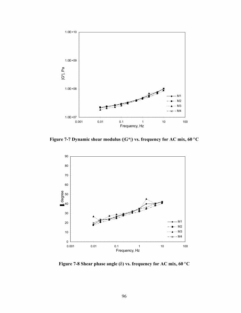
96
1.0E+07
1.0E+08
1.0E+09
1.0E+10
0.001 0.01 0.1 1 10 100Frequency, Hz
|G*|,
Pa
M1M2M3M4
Figure 7-7 Dynamic shear modulus (|G*|) vs. frequency for AC mix, 60 °C
0
10
20
30
40
50
60
70
80
90
0.001 0.01 0.1 1 10 100Frequency, Hz
, deg
ree
M1M2M3M4
Figure 7-8 Shear phase angle (δ) vs. frequency for AC mix, 60 °C

97
1.0E+07
1.0E+08
1.0E+09
1.0E+10
0.001 0.01 0.1 1 10 100Frequency, Hz
|G*|,
Pa
20 C30 C40 C60 C
Figure 7-9 Average dynamic shear modulus (|G*|) vs. frequency for AC mix
0
10
20
30
40
50
60
70
80
90
0.001 0.01 0.1 1 10 100Frequency, Hz
, deg
ree
20 C30 C40 C60 C
Figure 7-10 Average shear phase angle (δ) vs. frequency for AC mix

98
1.0E+06
1.0E+07
1.0E+08
1.0E+09
1.0E+10
0.00001 0.0001 0.001 0.01 0.1 1 10 100 1000 10000
Reduced Frequency, Hz
|G*|,
Pa
20 C30 C40 C60 C
Figure 7-11 |G*| master curve for AC mix, 30 °C
0
10
20
30
40
50
60
70
80
90
0.00001 0.0001 0.001 0.01 0.1 1 10 100 1000 10000
Reduced Frequency, Hz
, deg
rees
20 C30 C40 C60 C
Figure 7-12 Shear phase angle (δ) master curve for AC mix, 30 °C

99
1.0E+06
1.0E+07
1.0E+08
1.0E+09
1.0E+10
0.00001 0.0001 0.001 0.01 0.1 1 10 100 1000 10000
Reduced Frequency, Hz
|G*|,
Pa
20 C30 C40 C60 C
Figure 7-13 |G*| master curve for AC mix, 40 °C
0
10
20
30
40
50
60
70
80
90
0.00001 0.0001 0.001 0.01 0.1 1 10 100 1000 10000
Reduced Frequency, Hz
, deg
rees
20 C30 C40 C60 C
Figure 7-14 Shear phase angle (δ) master curve for AC mix, 40 °C

100
1.0E+06
1.0E+07
1.0E+08
1.0E+09
1.0E+10
0.00001 0.0001 0.001 0.01 0.1 1 10 100 1000 10000
Reduced Frequency, Hz
|G*|,
Pa
30 C40 C
Figure 7-15 |G*| master curve for AC mix, 30 and 40 °C
0
10
20
30
40
50
60
70
80
90
0.00001 0.0001 0.001 0.01 0.1 1 10 100 1000 10000
Reduced Frequency, Hz
, deg
rees
30 C40 C
Figure 7-16 Shear phase angle (δ) master curve for AC mix, 30 and 40 °C

101
1.0E-04
1.0E-03
1.0E-02
1.0E-01
1 10 100 1000 10000 100000Number of Cycles
Pla
stic
She
ar S
train
M1 - 60 C
M2 - 60 C
M3 - 40 C
M4 - 40 C
Figure 7-17 Plastic shear strain vs. RSCH cycles, 40 and 60 °C for AC mixes
1.0E+07
1.0E+08
1.0E+09
1.0E+10
0.1 1 10 100
Frequency (Hz)
|E*|,
Pa sa07- 20C
sa12 - 20 Csa07 - 30 Csa12 - 30 Csa07 - 40 Csa12 - 40 Csa07 - 60 Csa12 - 60 C
Figure 7-18 Dynamic axial modulus (|E*|) vs. frequency for AC mix

102
1.0E+07
1.0E+08
1.0E+09
1.0E+10
0.1 1 10 100
Frequency (Hz)
|E*|,
Pa
20c30c40c60c
Figure 7-19 Average dynamic axial modulus (|E*|) vs. frequency for AC mix
0
10
20
30
40
50
60
70
80
90
0.1 1 10 100
Frequency (Hz)
, deg
ree
20c
30c
40c
60c
Figure 7-20 Average axial phase angle (δ) vs. frequency for AC mix

103
1.0E-05
1.0E-04
1.0E-03
1.0E-02
1.0E-01
1 10 100 1000 10000 100000Number of Cycles
Pla
stic
Axi
al S
train
SA04 - 40CSA05 - 40 CSA01 - 60 CSA03 - 60 C
Figure 7-21 Plastic axial strain vs. cycles, 40 and 60 °C for AC mixes
y = 3.3718xR2 = 0.9914
0.E+00
1.E+05
2.E+05
3.E+05
4.E+05
5.E+05
6.E+05
7.E+05
8.E+05
9.E+05
1.E+06
0.E+00 5.E+04 1.E+05 2.E+05 2.E+05 3.E+05 3.E+05
|G*|, psi
|E*|,
psi
Figure 7-22 Relationship between |G*| and |E*| for AC mixes

104
y = 0.9738xR2 = 0.8812
0
10
20
30
40
50
60
0 10 20 30 40 50 60
Shear phase angle, deg.
Axi
al p
hase
ang
le, d
eg.
Figure 7-23 Relationship between shear and axial phase angle for AC mixes
Figure 7-24 Set up for elastic modulus of concrete using a 6×12 cylinder

105
y = 3E+06x + 38.218R2 = 0.9965
0
200
400
600
800
1000
1200
0.E+00 5.E-05 1.E-04 2.E-04 2.E-04 3.E-04 3.E-04 4.E-04 4.E-04
Strain
Stre
ss, p
si
Figure 7-25 Axial stress vs. strain at 7 days for PCC
0
20
40
60
80
100
0.01 0.1 1 10 100
Sieve Size, mm
Per
cent
Pas
sing
#67ScrgsCombined
Figure 7-26 Gradation of materials used for CTB

106
135.00
140.00
145.00
150.00
3.00 3.50 4.00 4.50 5.00 5.50 6.00 6.50 7.00 7.50
Moisture Content, %
Dry
Uni
t Wei
ght,
pcf
Figure 7-27 Moisture density curve for CTB
Figure 7-28 Resilient modulus of cement treated bases (CTB), [1, 14]
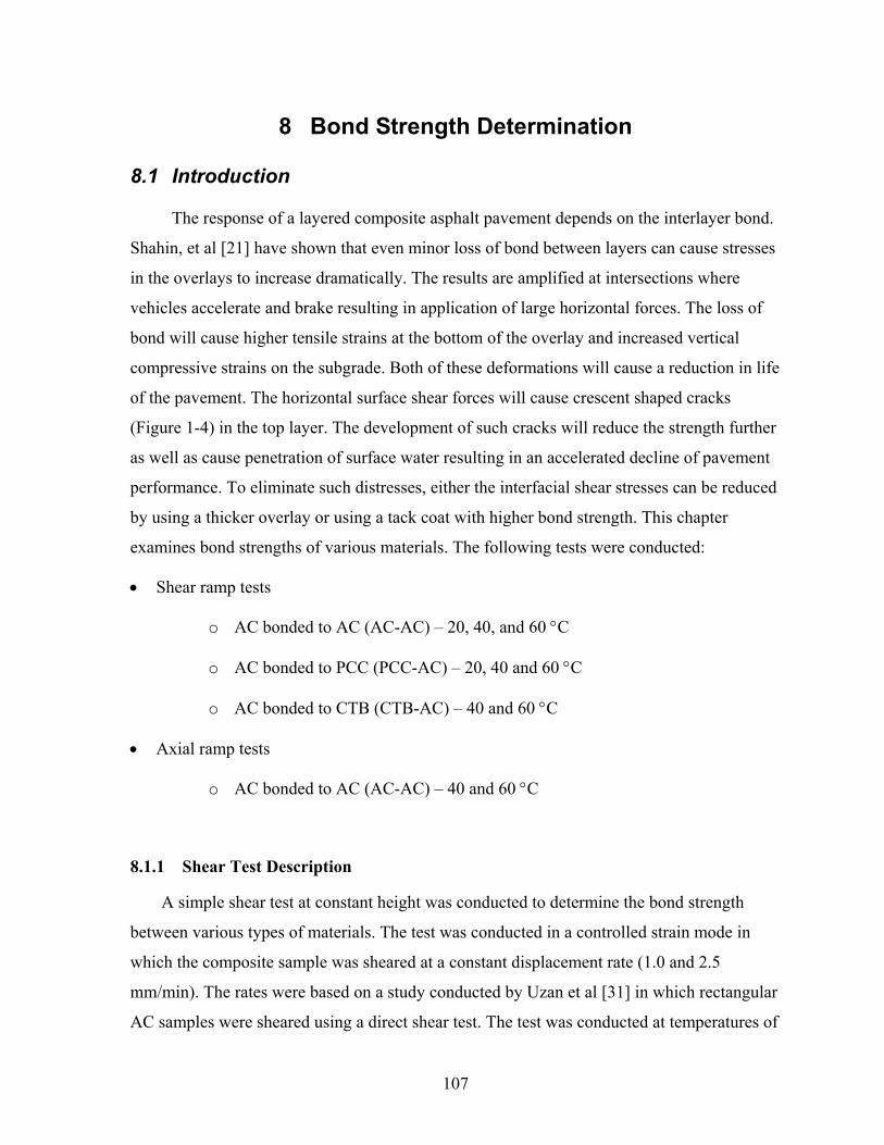
107
8 Bond Strength Determination
8.1 Introduction
The response of a layered composite asphalt pavement depends on the interlayer bond.
Shahin, et al [21] have shown that even minor loss of bond between layers can cause stresses
in the overlays to increase dramatically. The results are amplified at intersections where
vehicles accelerate and brake resulting in application of large horizontal forces. The loss of
bond will cause higher tensile strains at the bottom of the overlay and increased vertical
compressive strains on the subgrade. Both of these deformations will cause a reduction in life
of the pavement. The horizontal surface shear forces will cause crescent shaped cracks
(Figure 1-4) in the top layer. The development of such cracks will reduce the strength further
as well as cause penetration of surface water resulting in an accelerated decline of pavement
performance. To eliminate such distresses, either the interfacial shear stresses can be reduced
by using a thicker overlay or using a tack coat with higher bond strength. This chapter
examines bond strengths of various materials. The following tests were conducted:
• Shear ramp tests
o AC bonded to AC (AC-AC) – 20, 40, and 60 °C
o AC bonded to PCC (PCC-AC) – 20, 40 and 60 °C
o AC bonded to CTB (CTB-AC) – 40 and 60 °C
• Axial ramp tests
o AC bonded to AC (AC-AC) – 40 and 60 °C
8.1.1 Shear Test Description
A simple shear test at constant height was conducted to determine the bond strength
between various types of materials. The test was conducted in a controlled strain mode in
which the composite sample was sheared at a constant displacement rate (1.0 and 2.5
mm/min). The rates were based on a study conducted by Uzan et al [31] in which rectangular
AC samples were sheared using a direct shear test. The test was conducted at temperatures of

108
40 and 60 °C, and in some cases at 20 °C. The composite samples were glued to metal
platens and were sheared at constant height in the SST. The peak shear load per unit area was
the failure shear strength. Axial load and displacement were monitored during the test. The
specimens were sheared to a displacement of 5-mm.
8.2 Bond Strength using Metal Platens
Metal platens (anodized aluminum) were used to determine the bond strength of tack
and prime coat emulsions. Tack coat was applied to the one of the platens at the standard rate
of 0.06 gallons per square yard. Using the gluing jig for SST specimens, the two platens were
aligned and a minimal axial pressure of 10 psi was applied to keep them in contact. After 8
hours, the platens were removed from the jig and left in a draft oven at 40 °C to break the
emulsions. Twenty four hours after gluing; the platens were sheared using the SST machine
at shear displacement rates of 1.0 and 2.5 mm per minute. The test results were highly
variable and the entire procedure was error prone due to following reasons:
• At the time of coating, the emulsions were in an unbroken state and, therefore, very fluid.
When the two platens were pressed against each other, the liquid emulsion tended to
ooze out from the sides. This changed the effective rate of application of tack coat and
ultimately the interlayer asphalt film thickness available for bonding.
• When the platens were pressed against each other, the water from the emulsion was
trapped in between the two impervious platens. The trapped water could, potentially,
adversely affect the bond strength. This is not the case with bonded AC, PCC or CTB
specimens as the emulsions are allowed to break.
• When the platens were inserted into the SST and clamped, they tended to separate before
testing. This was due to presence of inadequately cured tack coats or due to high forces
applied by the SST or extremely low strength of the tack coat.
• An alternative approach attempted was to allow the emulsion to break on one of the
platens and, after 24 hours, bond it with another platen. But this approach had similar
problems. At the pavement interface, the asphalt penetration into adjacent layers

109
provides a stronger bond compared to the bond developed between two impervious
platens.
• The relative strength of any tack (or prime) coat, by itself, is small when compared to the
interfacial strength of a composite pavement specimen it helps bond together. The use
of heavy metal platens and SST to test the strength of tack (or prime) coats yielded
erroneous results due to noise and low sensitivity of the equipment. A better alternative
would be to use platens comparable to the size of a DSR spindle and a sensitive
machine. An alternative is to use ATACKER™3 device that uses a light weight
aluminum spindle (sizes – 1, 2, and 4 inch in diameter) and a dial gauge that can
measure the load to ½ lb accuracy. The set up is similar to DSR. The specimens are
sheared or pulled apart in a strain-controlled mode and the load at which the two plates
separate is noted as the bond strength.
Overall, the results from these tests did not contribute much to this study due to
practical problems encountered in the testing protocol.
8.3 Bond Strength of AC-AC specimens
8.3.1 Axial and Shear Ramp Test
Axial ramp test is similar to the simple shear test, except that the load is applied axially
in controlled strain mode. Similarly, for shear ramp test, the samples were sheared at a
constant strain rate. The rate of displacement used for axial and shear tests was 1 and 2.5
mm/minute. The axial test is used to measure the adhesion of the interfaces glued by a tack
coat whereas the shear test measures the interfacial shear resistance. The specimens used
were 2-inch thick and 6-inch in diameter with interface between the two layers roughly at
mid-height. This test was performed on composite asphalt concrete specimens (AC bonded to
AC) to determine the effectiveness of PG64-22 versus CMS-2 as a tack coat. Control
specimens were also prepared without using a tack coat. However, during the coring and
cutting process, control samples (Figure 8-1) made without any tack coat separated at the
interface and, therefore, could not be tested.
3 ATACKER™ is equipment developed by Instrotek Inc, of Raleigh, NC.

110
8.3.2 Axial Test Results
The axial test results are presented in Table 8-1 and Table 8-2. It can be seen that low
strain rate produces lower peak load values. For CMS-2 at 40 °C, when the displacement rate
reduces from 2.5 mm/minute to 1.0 mm/minute, the shear strength changes from 221 to 95
psi – a reduction of 57%. Similarly, for CMS-2, the reduction in peak axial strength when
tested at a lower rate of 1 mm/minute is 48 percent at 60 °C. Comparing the axial test data for
40 and 60 °C, for CMS-2, (Table 8-1 and Table 8-2) the peak axial stress falls with rise in
temperature. When the temperature increases from 40 to 60 °C, the peak axial strength
reduces by 85% and 75% for 1.0 and 2.5 mm/min displacement rates respectively.
For the same axial displacement rates, the corresponding peak load values and axial
strains are much higher for PG64-22 binder than the CMS-2 emulsion. This suggests that
PG64-22 binder has a higher axial strength than CMS-2 emulsion at both temperatures. This
is expected because:
• Amount (wt/sq. yd) of residual asphalt available at the interface is higher for PG64-22
binder than for CMS-2 emulsion (which as about 33%) water.
• In addition, the PG rating of the residual asphalt in CMS-2 is PG52 (Table 4-2).
The failure of CMS-2 tacked specimens in axial testing mode was observed to be at the
interface as shown in Figure 8-2 and Figure 8-3; however for PG64-22 tacked specimens the
failure was not well defined as CMS-2 tacked specimens, as shown in Figure 8-4 and Figure
8-5. This observation confirms that PG64-22 provides better adhesion than CMS-2 emulsion.
8.3.3 Shear Test Results
The results for shear tests are presented in Table 8-3 through Table 8-5. The test was
conducted in a constant height mode to simulate the confinement observed in situ. Negative
axial stresses shown in the tables indicate compressive load and are due to prevention of
dilation of specimens during the shearing process. The pattern for shear failure varies
depending on the testing temperature and rate of shear. The test results are graphically

111
presented in Figure 8-6 through Figure 8-8. The failure pattern (Figure 8-9 through Figure
8-12) observed for the shear test at 40 °C is similar to that of a monolithic sample – there was
a development of a crack along the principal diagonal, typical of a shear failure for, both,
CMS-2 and PG64-22 tacked specimens. This indicated that the bond was as strong as the mix
at 40 °C. From Table 8-3 to Table 8-5, it can be seen that there is very little difference in the
bond strength of specimens tacked with CMS-2 and PG64-22, especially at a higher
displacement rate of 2.5 mm/minute. There is a small difference in bond strength at lower
strain rate of 1 mm/minute with the average (across all temperatures) difference in general
being about 14% with PG64-22 tacked specimens showing higher bond strength.
For CMS-2 tacked specimens the interfacial failure was observed regardless of the rate
of shear displacement at 20 °C. For PG64-22, at 20 °C, failure at lower displacement rate was
monolithic (Figure 8-13) but at higher displacement rate the failure was interfacial (Figure
8-14). At 20 °C and 1-mm/minute displacement rate, the peak bond strength of CMS-2 is
lower than PG64-22 by 8%.
The shear strength values drop drastically at 60 °C, with PG64-22 specimens
performing marginally better than CMS-2 specimens. A higher displacement rate produces a
higher strength as is clear from data in Table 8-5. The difference between the shear strengths
of PG64-22 and CMS-2 emulsion is 9% and 45% at displacement rates of 1.0 and 2.5
mm/min. Referring to Figure 8-6 and Figure 8-7, it can be seen that failures occur rapidly
under higher displacement rates than compared to lower strain rates. Further, the occurrence
of peak load shifts to the right with increase in temperature and reduction of displacement
rate – a phenomenon occurring due to mix getting softer. The failure of composite specimens
at 60 °C was observed to be at the interface suggesting that the bond was the weakest link at
that temperature.
Figure 8-8 shows the summary of bond strength as function of temperature. It can be
seen from this figure that, in general, the CMS-2 bond strength is not very much different
compared to PG64-22. From Figure 8-8, the bond strength values at 25 °C, for CMS-2 and
PG64-22 tacked specimens is 960 and 1020 kPa respectively (at displacement rate of 1.0
mm/minute). Studies by Sholar et al [24] measured the bond strengths of various AC-AC
interfaces in shear at 25 °C at different time intervals. The AC-AC samples were sheared at a

112
constant displacement rate of 19.1 mm/minute. Table 8-6 shows the bond strengths (in shear)
for various sections, from Sholar et al [24], in the last round of testing. The values are then
interpolated to obtain the strength at an application rate of 0.06 gal./yd2 (0.272 L/m2). The
interpolated bond strengths (in shear) range from 921 to 1011 kPa which is fairly close to the
values obtained from Figure 8-8 (960 and 1020 kPa).
8.4 Bond Strength of PCC-AC specimens
The composite specimens of PCC and AC were tested in shear using the ramp tests
described earlier. The testing was conducted at 20, 40 and 60 °C. In all, three cases were
considered: no tack coat, PG64-22 binder as tack coat and CMS-2 emulsion as tack coat. For
specimens prepared without tack coat, immediately after curing and drying the slab, the
surface of PCC slab was cleaned and an asphalt layer was paved on the PCC slab. While
dismantling the mold and coring the slab, the two layers of AC and PCC tended to separate
(Figure 8-15 and Figure 8-16). The black slab is the asphalt concrete slab paved on top of the
white PCC slab. This occurred on two attempts and it was evident that bond formation did
not occur between these two layers.
For composite specimens tacked with PG64-22 binder and CMS-2 emulsion, the shear
results are listed in Table 8-7 through Table 8-9, and Figure 8-17 through Figure 8-19. The
behavior of PCC-AC interface bond is the property of tack coat as well as the asphalt mix;
PCC only serves as a rigid layer to which the AC is tacked as the PCC stiffness is much
higher than the AC mix. As a consequence, the aggregates from AC layer do not get to
penetrate into the voids of the PCC layer increasing the likelihood of lower bond strength.
The properties of PCC do not change significantly with temperature or rate of shear. It can be
seen that with increasing temperature, the bond strength continues to reduce.
For PCC-AC specimens, PG64-22 composite specimens have slightly lower shear
strengths at a displacement rate of 1.0 mm/min compared to CMS-2. However, the trend at
higher strain rates reflects PG64-22 as a stronger tack coat. It can be argued that the bond
strength of PG64-22 is very close to the actual mix strength at lower strain rates and,
therefore, CMS-2, PG64-22 rate equally well in shear strength. The CMS-2 bond strength,

113
however, is lower than PG64-22 by 2.5%, 17.9%, and 31.8% (displacement rate of
2.5mm/min) at 20, 40, and 60 °C respectively. The difference in the shear strengths
progressively widens with increasing temperature, between PG64-22 and CMS-2 at higher
temperatures. With increasing temperatures, the development of peak shear stress (Figure
8-17 and Figure 8-18) gets less clearly defined. At 20 °C the peaks for CMS-2 and PG64-22
are clearly defined; at 40 °C the peaks are not as clearly defined and at 60 °C they cannot be
identified at all. This is due to progressive weakening of the bond strength between PCC and
AC. Further, the failure (signified by occurrence of peak) is instantaneous and well-defined
at lower temperatures whereas at higher temperatures it is gradual. Most of the specimens,
regardless of the tack coat, show a clear-cut slipping at the interface. While the PCC layer
has been minimally affected, cracks developed in the AC layer for interfaces tacked with
PG64-22 as is evident in Figure 8-20. It suggests that the strength of PG64-22 bond is at least
as strong as the mix. In case of CMS-2 specimens, the failure was at the interface for all the
specimens. Figure 8-21 shows a failed PCC-AC composite tacked with CMS-2. The
deformation in AC was negligible with all slippage occurring at the interface suggesting
bond strength as the weakest link.
Studies conducted by Mukhtar and Dempsey [19] tested composite PCC-AC
specimens (Figure 1-11) at a constant displacement rate of 1.0, 3.0 and 300 inch per minute.
Table 8-10 and Figure 8-22 summarize the strengths obtained at various temperatures at an
axial confining pressure of 79 psi. Comparing the values at 20 °C, from Figure 8-22, it can be
seen that the interfacial shear strengths are about 750, 1125 and 1750 kPa at displacement
rates of 1, 30, and 300 inch per minute. The shear strength (~750 kPa) at 1.0 inch per minute
displacement rate at 20 °C is about twice the value obtained under this study (Table 8-7). It
can be observed (Table 8-7) that the maximum axial stress mobilized during the PCC-AC
testing was 20 psi compressive. Thus the effect of axial confinement could have contributed
to higher shear strengths in case of Mukhtar and Dempsey [19].
The bond strengths of PCC-AC composite specimens are lower than the corresponding
strengths of AC-AC except at 60 °C. Thus, keeping everything else equal, dissimilar surfaces
(like PCC and AC) produce a weaker bond compared to bond between similar surfaces (AC-
AC). The difference between the dynamic moduli of PCC and AC could be a contributory

114
factor to the lower strength of the interface. Further, the PCC layer being relatively
impervious, the tack coat does not penetrate into it potentially affecting the bond strength. In
case of AC-AC interfaces, the elevated temperature of the overlay mix during the paving
process could cause the underlying layer to soften up causing them to fuse and thereby
enhancing the bond strength. Overall, based on the data it can be concluded that PG64-22
performs marginally better than CMS-2 emulsion when used to bond PCC and AC. Figure
8-19 summarizes the bond strength as a function of temperature.
8.5 Bond Strength of CTB-AC specimens
This section deals with the shear strength of composite specimens (Figure 8-23) made
of CTB and AC. The testing was carried out at 40 and 60 °C at shear displacement rates of
1.0 and 2.5 mm per minute at constant height. Three types of emulsions – CSS-1h, EA-P and
EPR-1 – were used as prime coats. In addition, composite CTB-AC samples without any
prime coat were manufactured to be used as a control case. The performance of unprimed
CTB-AC samples was similar to non-tacked composite (AC-AC and PCC-AC) specimens.
The bond formation between CTB and AC was not strong enough to withstand the handling
stresses. After extruding the samples from gyratory molds, AC and CTB layers could be
easily pulled apart by hand. The results from the tests for primed samples are summarized in
Table 8-12 and Table 8-12, and Figure 8-24 through Figure 8-27.
It should be noted that unlike AC-AC and PCC-AC, the CTB-AC specimens show
decreasing shear bond strength with increasing applied shear strain rate. The CTB has very
low strength and brittle behavior. During the shearing process it is possible that aggregates
near the interface from the CTB must be loosened and reoriented causing dilation of the
specimen. As the test was carried out at constant height, the loosening of aggregates and
subsequent dilation could cause a jump in axial stresses. These increased axial stresses lead
to an increase in the shear resistance of the interface. The behavior (Figure 8-24 through
Figure 8-26) of CTB-AC interface when subjected to a shear strain (at constant height) shows
substantially higher shear strengths compared to AC-AC and PCC-AC composite specimens.

115
At 40 °C, CSS-1h performs better than the other two prime coats, EA-P and EPR-1.
The strengths of EA-P and EPR-1, at 40 °C, are 30.9% and 17.2% lower than CSS-1h at a
displacement rate of 1.0 mm per minute. At a higher displacement rate (2.5 mm per minute)
and at 40 °C, the shear strengths of EA-P and EPR-1 are 41.6% and 2.8% lower than CSS-
1h. Based on shear strengths at 40 °C, the prime coats with decreasing order of shear
strengths can be rated as CSS-1h, EPR-1, and EA-P. Another observation is that, at 40 °C,
the reduction in strength with increasing rate of shear displacement (from 1.0 to 2.5 mm per
minute) is 25.6%, 37.1% and 12.7% for CSS-1h, EA-P, and EPR-1 respectively. The reason,
perhaps, would be due to inadequate time for development of aggregate interlock owing to
faster interlayer movement. Observation of tested CSS-1h (at 40 °C) samples indicated a
failure pattern consistent with a monolithic specimen. No debonding or layer separation was
observed and diagonal cracks were seen in AC and CTB (Figure 8-28). For EA-P specimens
(at 40 °C), diagonal cracking in AC as well as a shear failure at interface was observed but
for EPR-1 only interfacial shear with minor cracking in the AC layer was observed.
At 60 °C, the EA-P primed specimens show a high degree of variability. Indeed the
strength was so low that the specimens could be de-bonded by hand (Figure 8-30). Therefore,
these results were discarded. At 60 °C, CSS-1h bond strength is higher than EPR-1 at 2.5 mm
per minute rate of shear. The failure pattern observed for CSS-1h specimens at 60 °C was
similar to the pattern observed at 40 °C. For EA-P and EPR-1 specimens the failure was due
to interlayer debonding (Figure 8-29, Figure 8-30). The shear strengths at 60 °C are
comparable to shear strengths at 40 °C for CSS-1h and EA-P. That means it is possible that
the rough CTB surface plays a greater role compared to the bonding agent, especially under
axial confinement.
Based on the test results, it can be concluded that priming does increase the bond
between the CTB and the AC layer; however temperature plays only a minor role. The
mobilization of bond strength appears to be primarily due to a combination of prime coat
adhesion and more importantly aggregate interlock. Figure 8-27 summarizes the results for
bond strength versus temperature.

116
8.6 Summary and Conclusions
The objective of this task was to evaluate the performance of composite samples made
by bonding AC-AC, PCC-AC and CTB-AC. Of particular interest was the effect of type of
tack coat and test temperatures. The observations and conclusions from the bond strength
determination tests are summarized below:
1. The shear and axial ramp tests clearly differentiate between the bond strengths of various
tack and prime coats. The numbers from these tests are consistent with the visually
observed failure pattern of the test specimens.
2. The problems encountered in testing the bond strength of the tack (or prime) coat using
SST metal platens were due to size effects, loss of asphalt from sides, and problems in
curing the emulsions. The heavy weight of platens and low sensitivity of SST vis-à-vis
low strength of asphalt posed hurdles to get meaningful results. A better alternative
would be to use a device like Atacker™ to measure the adhesion properties where the
size of equipment is small and the accuracy higher.
3. The absence of tack or prime coat would severely hinder development of bond between
two layers causing undue slippage. This is evident from the debonding that occurred
between non-tacked AC-AC, PCC-AC and CTB-AC interfaces.
4. For AC-AC composites the strength of PG64-22 binder, when used as a tack coat,
provides comparable adhesion to CMS-2 emulsion. This is supported by similar axial and
shear strengths of PG64-22 tacked specimens compared to CMS-2 tacked specimens.
5. For PCC-AC composites, the results confirm the earlier observation that CMS-2 provides
comparable adhesion to PG64-22.
6. The bond between two similar surfaces (AC-AC vis-à-vis PCC-AC) is stronger than the
bond between two dissimilar surfaces. Further the absorption of emulsion into underlying
AC layer and the increased chance for aggregate interlock could potentially contribute to
the higher strength of AC-AC interface compared to that of PCC-AC interface.
7. CSS-1h performs better than EA-P and EPR-1 as prime coats. The apparent strength of
CTB-AC bond is higher due to the dilation of composite specimens. The strength of
CTB-AC composites appears to be influenced significantly by the aggregate interlock.

117
Overall, the relative performance of various tack and prime coats could be determined based
on SST tests. Emulsions, though easy to use, could pose problems if improperly applied or
cured prior to paving AC layer. The use of PG64-22 binder as a tack coat could not only
eliminate these problems but provide better bonding as well.
Table 8-1 Results for AC-AC axial ramp tests (tensile), 40 °C
Specimen ID
Height (mm)
Air voids (%)
Displ. Rate(mm/min) Tack Coat Peak Axial Stress
(kPa) Average Peak
Axial Stress (kPa)10c4 6-16-2 49.96 3.7 1.0 CMS-2 113.74 10x 6-16-2 50.48 3.6 1.0 CMS-2 76.64 95.19
25c4 6-3-2 51.36 3.9 2.5 CMS-2 307.80 25m2 6-16-2 50.93 3.8 2.5 CMS-2 134.78 221.28
10c4 4-15-2 52.65 3.6 1.0 PG64-22 145.17 10x 5-16-2 51.55 3.8 1.0 PG64-22 153.62 149.40
25m1 5-16-2 50.17 4.3 2.5 PG64-22 240.07 25m2 5-16-2 51.20 4.3 2.5 PG64-22 330.99 285.53
Table 8-2 Results for AC-AC axial ramp tests (tensile), 60 °C
Specimen ID
Height (mm)
Air voids (%)
Displ. Rate(mm/min) Tack Coat Peak Axial Stress
(kPa) Average Peak
Axial Stress (kPa)10m1 7-20-2 50.39 4.4 1.0 CMS-2 9.10 10m3 6-16-2 49.20 4.5 1.0 CMS-2 20.40 14.75
25c3 7-20-2 49.88 4.3 2.5 CMS-2 62.35 25x 7-20-2 50.95 4.5 2.5 CMS-2 52.03 57.19
10c2 4-15-2 48.47 4.5 1.0 PG64-22 19.16 10m4 5-16-2 50.83 4.5 1.0 PG64-22 22.58 20.87
25c2 5-16-2 49.56 4.2 2.5 PG64-22 59.06 25m3 9-3-2 49.05 4.3 2.5 PG64-22 81.52 70.29
Table 8-3 Results for AC-AC shear ramp tests, 20 °C
Specimen ID
Height (mm)
Air voids (%)
Displ. Rate
(mm/min)
Tack Coat
Axial Stress (kPa)
Peak Shear Stress (kPa)
Average Peak Shear Stress
(kPa) 1mmc2 49.91 4.3 1.0 CMS-2 -923.32 1098.39 1mmc3 50.73 4.4 1.0 CMS-2 -986.23 1057.48 1077.94
25mmm1 50.87 4.2 2.5 CMS-2 -967.73 1232.25 25mmm2 50.17 4.1 2.5 CMS-2 -729.49 961.49 1096.87
1mmc2 53.09 3.8 1.0 PG64-22 -894.55 1076.37 1mmc21 50.41 4.2 1.0 PG64-22 -1010.72 1277.65 1177.01
25mmm3 48.70 4.1 2.5 PG64-22 -53.67 617.61 25mmx 49.69 4.3 2.5 PG64-22 -58.47 634.26 625.94

118
Table 8-4 Results for AC-AC shear ramp tests, 40 °C
Specimen ID
Height (mm)
Air voids (%)
Displ. Rate
(mm/min)
Tack Coat
Axial Stress (kPa)
Peak Shear Stress (kPa)
Average Peak Shear Stress
(kPa) 10m1 6-16-2 49.58 4.2 1.0 CMS-2 -485.37 384.94 10m3 6-3-2 47.81 4.1 1.0 CMS-2 -652.51 512.20
448.57
25c1 6-3-2 51.58 4.1 2.5 CMS-2 -641.14 521.53 25c1_1 6-16-2 52.27 4.3 2.5 CMS-2 -560.57 436.78 479.16
10c3 4-15-2 51.05 3.9 1.0 PG64-22 -653.78 492.93 10m1 4-15-2 52.38 3.8 1.0 PG64-22 -504.93 409.11 451.02
25m1 5-7-2 51.91 3.7 2.5 PG64-22 -686.60 568.26 25m2 5-7-2 51.14 3.7 2.5 PG64-22 -662.86 539.79
554.03
Table 8-5 Results for AC-AC shear ramp tests, 60 °C
Specimen ID
Height (mm)
Air voids (%)
Displ. Rate(mm/min) Tack Coat Peak Shear Stress
(kPa) Average Peak
Shear Stress (kPa)10m1 6-3-2 51.74 3.6 1.0 CMS-2 0.84 10m4 6-16-2 50.29 3.5 1.0 CMS-2 5.08
2.96
25m2 7-20-2 51.07 3.7 2.5 CMS-2 4.62 25c2 7-20-2 49.83 4.2 2.5 CMS-2 9.42 7.02
10c3 5-7-2 50.04 3.5 1.0 PG64-22 5.78 10x 9-3-2 49.22 4.3 1.0 PG64-22 4.90 5.34
25m1 9-3-2 48.48 3.6 2.5 PG64-22 7.93 25c1 5-16-2 50.55 4.2 2.5 PG64-22 7.49
7.71
Table 8-6 Summary of shear strengths from Sholar et al, [24]
Measured Bond Strength (kPa) Section @0.226 L/sq. m @0.362 L/sq. m
Interpolated Bond Strength (kPa)@0.272 L/sq. m (0.06 gal/sq. yd)
US-90 1022 989 1011 I-95 non-milled 943 876 921
I-95 milled 1059 911 1009

119
Table 8-7 Results for PCC-AC shear ramp tests, 20 °C
Specimen ID
Height (mm)
Displ. Rate (mm/min) Tack Coat Axial Stress
(kPa) Peak Shear Stress
(kPa) Average Peak
Shear Stress (kPa)1mm7 51.21 1.0 CMS-2 58.13 235.05 1mm8 49.54 1.0 CMS-2 -22.84 429.26 332.16
25mm6 50.87 2.5 CMS-2 -40.62 109.51 25mm9 53.58 2.5 CMS-2 -110.03 611.86 360.18
1mm6 50.91 1.0 PG64-22 -53.12 446.89 1mm16 48.01 1.0 PG64-22 -85.46 102.03 1mm18 47.40 1.0 PG64-22 -140.10 123.42
224.11
25mm14 50.07 2.5 PG64-22 -132.47 226.04 25mm8 50.18 2.5 PG64-22 -70.23 501.88 363.96
Table 8-8 Results for PCC-AC shear ramp tests, 40 °C
Specimen ID
Height (mm)
Displ. Rate (mm/min) Tack Coat Axial Stress
(kPa) Peak Shear Stress
(kPa) Average Peak
Shear Stress (kPa)1mm12 48.95 1.0 CMS-2 -108.48 78.11 1mm13 50.35 1.0 CMS-2 -27.92 48.82 63.47
25mm11 46.87 2.5 CMS-2 -38.19 121.31 25mm14 49.90 2.5 CMS-2 -115.57 91.38 106.35
1mm04 52.54 1.0 PG64-22 -73.38 78.32 1mm13 49.72 1.0 PG64-22 -49.39 45.78 62.05
25mm02 52.46 2.5 PG64-22 -9.13 99.03 25mm10 49.74 2.5 PG64-22 -114.73 160.11 129.57
Table 8-9 Results for PCC-AC shear ramp tests, 60 °C
Specimen ID
Height (mm)
Displ. Rate (mm/min) Tack Coat Axial Stress
(kPa) Peak Shear Stress
(kPa) Average Peak
Shear Stress (kPa)1mm04 50.07 1.0 CMS-2 -17.18 21.64 1mm10 51.80 1.0 CMS-2 -29.01 28.61 25.13
25mm01 50.74 2.5 CMS-2 -17.853 19.15 25mm02 49.84 2.5 CMS-2 -14.92 21.60 20.38
1mm07 49.80 1.0 PG64-22 -8.58 13.74 1mm15 44.69 1.0 PG64-22 -25.02 28.11 20.93
25mm01 49.91 2.5 PG64-22 -9.63 18.13 25mm12 50.63 2.5 PG64-22 -54.42 41.59 29.86

120
Table 8-10 Summary of PCC-AC bond strengths, [19]
Shear Displacement Rate Temperature (°F)
Temperature(°C) 1 in./min 30 in./min. 300 in./min
0 -17.78 882.5 806.7 703.3 20 -6.67 1234.2 1275.5 1268.6 40 4.44 1213.5 1316.9 1599.6 60 15.56 848.1 1206.6 1840.9 80 26.67 606.7 992.8 1482.4
100 37.78 461.9 675.7 903.2
Table 8-11 Results for CTB-AC shear ramp tests, 40 °C
Specimen ID
Height (mm)
Displ. Rate (mm/min) Tack Coat Axial Stress
(kPa) Peak Shear Stress
(kPa) Average Peak
Shear Stress (kPa)1mm06 50.34 1.0 CSS-1h -433.95 353.52 1mm10 50.42 1.0 CSS-1h -454.80 381.46 367.49
25mm07 51.01 2.5 CSS-1h -384.17 328.16 25mm09 50.27 2.5 CSS-1h -252.53 218.31 273.23
1mm12 52.87 1.0 EA-P -262.10 201.83 1mm02 52.01 1.0 EA-P -421.71 305.80
253.82
25mm03 54.56 2.5 EA-P -237.98 155.92 25mm13 51.15 2.5 EA-P -244.48 163.32 159.62
1mm02 51.12 1.0 EPR-1 -305.84 225.03 1mm04 50.22 1.0 EPR-1 -465.11 351.91 1mm05 51.37 1.0 EPR-1 -429.51 336.19
304.38
25mm03 52.51 2.5 EPR-1 -397.30 280.99 25mm99 52.54 2.5 EPR-1 -336.37 250.31
265.65
Table 8-12 Results for CTB-AC shear ramp tests, 60 °C
Specimen ID
Height (mm)
Displ. Rate (mm/min) Tack Coat Axial Stress
(kPa) Peak Shear Stress
(kPa) Average Peak
Shear Stress (kPa)1mm01 50.27 1.0 CSS-1h -464.15 343.00 1mm05 51.51 1.0 CSS-1h -414.71 312.19 327.60
25mm02 50.54 2.5 CSS-1h -439.87 308.00 25mm08 53.78 2.5 CSS-1h -368.20 269.16 288.58
1mm10 50.75 1.0 EA-P -548.90 390.34 1mm11 54.85 1.0 EA-P -653.41 427.53 408.94
25mm08 50.84 2.5 EA-P -73.04 66.93 25mm11 54.85 2.5 EA-P -338.59 240.37 153.95
1mmOA 50.39 1.0 EPR-1 -256.48 177.18 1mmOI 51.39 1.0 EPR-1 -389.84 259.35 218.27
25mmOQ 52.65 2.5 EPR-1 -209.00 134.49 25mm01 53.12 2.5 EPR-1 -312.59 258.29 25XOC 51.46 2.5 EPR-1 -197.55 135.59
176.12
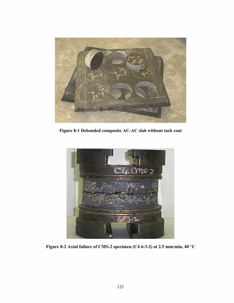
121
Figure 8-1 Debonded composite AC-AC slab without tack coat
Figure 8-2 Axial failure of CMS-2 specimen (C4 6-3-2) at 2.5 mm/min, 40 °C

122
Figure 8-3 Axial failure of CMS-2 specimen (C4 6-3-2) at 2.5 mm/min, 40 °C
Figure 8-4 Axial failure of PG64-22 specimen (M1 5-16-2) at 2.5 mm/min, 40 °C

123
Figure 8-5 Axial failure of PG64-22 specimen (M1 5-16-2) at 2.5 mm/min, 40 °C
0
200000
400000
600000
800000
1000000
1200000
0 100 200 300 400 500
Time (s)
She
ar S
tress
(Pa)
CMS, 1mm, 20CCMS, 2.5mm, 20CCMS, 1mm, 40CCMS, 2.5mm, 40C
Figure 8-6 Average shear stress vs. time for AC-AC interface tacked with CMS-2

124
0
200000
400000
600000
800000
1000000
1200000
1400000
0 100 200 300 400 500
Time (s)
She
ar S
tress
(Pa)
PG, 1mm, 20CPG, 2.5mm, 20CPG, 1mm, 40CPG, 2.5mm, 40C
Figure 8-7 Average shear stress vs. time for AC-AC interface tacked with PG64-22
0
200
400
600
800
1000
1200
1400
0 10 20 30 40 50 60 70
Temperature, C
She
ar S
treng
th, k
Pa
AC, CMS, 1mmAC, CMS, 2.5mmAC, PG, 1mmAC, PG, 2.5mm
Figure 8-8 Summary of bond strengths for AC-AC interface

125
Figure 8-9 Shear failure of CMS-2 specimen (m1 6-16-2) at 1.0mm/min, 40 °C
Figure 8-10 Shear failure of CMS-2 specimen (m3 6-3-2) at 1.0mm/min, 40 °C

126
Figure 8-11 Shear failure of CMS-2 specimen (c1 6-3-2) at 2.5mm/min, 40 °C
Figure 8-12 Shear failure of PG64-22 specimen (m1 5-7-2) at 2.5 mm/min, 40 °C

127
Figure 8-13 Shear failure of PG64-22 specimen (1mmc2_1) at 1.0 mm/min, 20 °C
Figure 8-14 Shear failure of PG64-22 specimen (25mmm3) at 2.5 mm/min, 20 °C
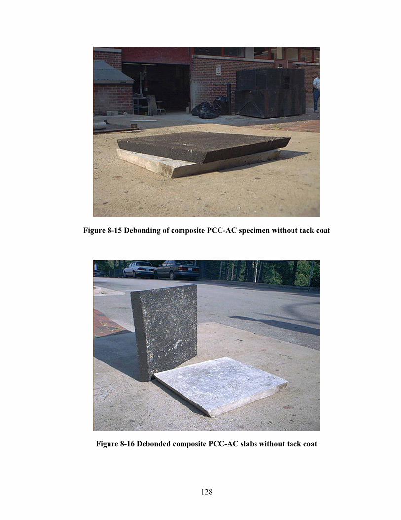
128
Figure 8-15 Debonding of composite PCC-AC specimen without tack coat
Figure 8-16 Debonded composite PCC-AC slabs without tack coat
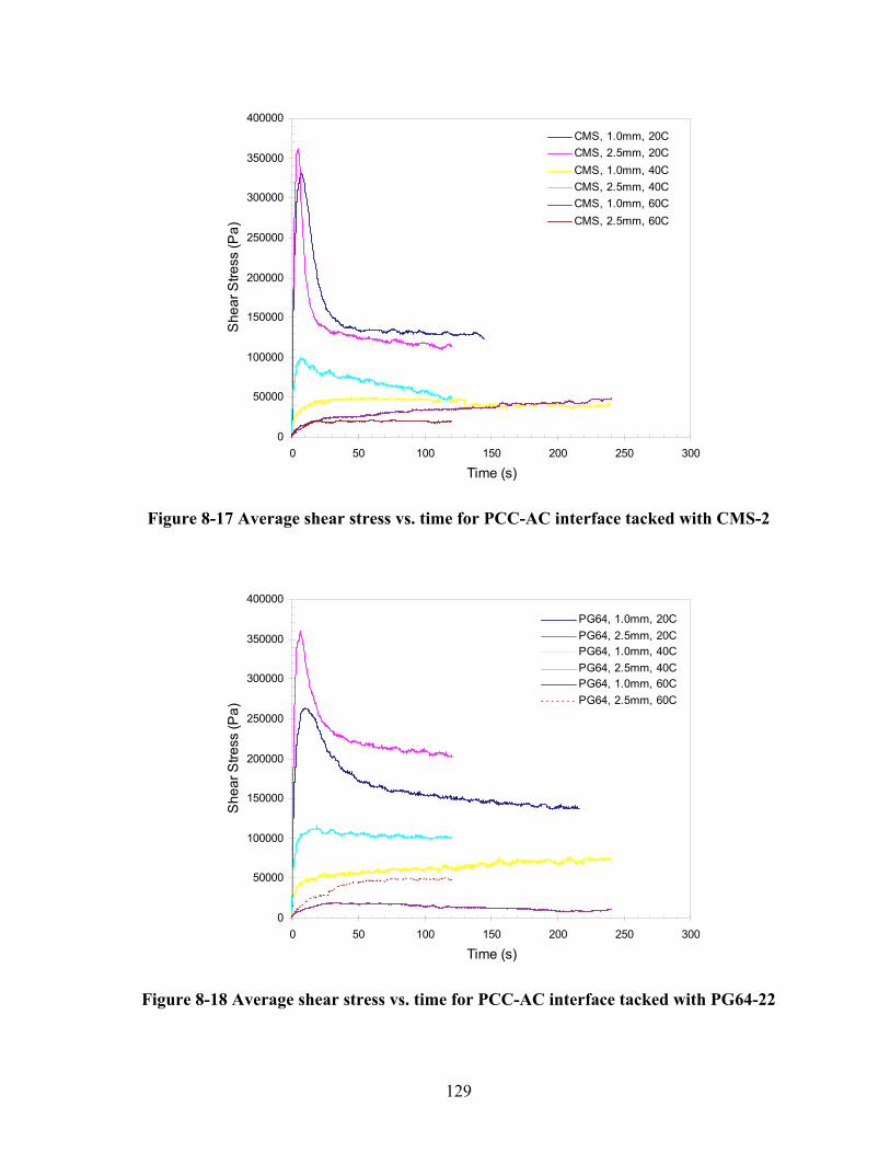
129
0
50000
100000
150000
200000
250000
300000
350000
400000
0 50 100 150 200 250 300
Time (s)
She
ar S
tress
(Pa)
CMS, 1.0mm, 20CCMS, 2.5mm, 20CCMS, 1.0mm, 40CCMS, 2.5mm, 40CCMS, 1.0mm, 60CCMS, 2.5mm, 60C
Figure 8-17 Average shear stress vs. time for PCC-AC interface tacked with CMS-2
0
50000
100000
150000
200000
250000
300000
350000
400000
0 50 100 150 200 250 300
Time (s)
She
ar S
tress
(Pa)
PG64, 1.0mm, 20CPG64, 2.5mm, 20CPG64, 1.0mm, 40CPG64, 2.5mm, 40CPG64, 1.0mm, 60CPG64, 2.5mm, 60C
Figure 8-18 Average shear stress vs. time for PCC-AC interface tacked with PG64-22

130
0
50
100
150
200
250
300
350
400
0 10 20 30 40 50 60 70
Temperature, C
She
ar S
treng
th, k
Pa
PCC, CMS, 1mmPCC, CMS, 2.5mmPCC, PG, 1mmPCC, PG, 2.5mm
Figure 8-19 Summary of bond strengths for PCC-AC interface
Figure 8-20 PCC-AC specimen tacked with PG64-22 (cracks highlighted in white)

131
Figure 8-21 PCC-AC specimen tacked with CMS-2
0
50
100
150
200
250
300
-20.00 -10.00 0.00 10.00 20.00 30.00 40.00 50.00
Temperature, C
She
ar S
treng
th, p
si
0.0
500.0
1000.0
1500.0
2000.0
-4 16 36 56 76 96 116Temperature, F
Stre
ngth
, kP
a
30in/min300in/min1in/min
Figure 8-22 Summary of PCC-AC shear bond strengths, [19]

132
Figure 8-23 Composite CTB-AC specimen
0
50000
100000
150000
200000
250000
300000
350000
400000
0 50 100 150 200 250 300
Time (s)
She
ar S
tress
(Pa)
CSS, 1mm, 40CCSS, 2.5mm, 40CCSS, 1mm, 60CCSS, 2.5mm, 60C
Figure 8-24 Average shear stress vs. time for CTB-AC interface primed with CSS-1h

133
0
50000
100000
150000
200000
250000
300000
350000
400000
450000
0 50 100 150 200 250 300
Time (s)
She
ar S
tress
(Pa)
EAP, 1mm, 40CEAP, 2.5mm, 40CEAP, 1mm, 60CEAP, 2.5mm, 60C
Figure 8-25 Average shear stress vs. time for CTB-AC interface primed with EAP
0
50000
100000
150000
200000
250000
300000
350000
0 50 100 150 200 250 300
Time (s)
She
ar S
tress
(Pa)
EPR, 1mm, 40CEPR, 2.5mm, 40CEPR, 1mm, 60CEPR, 2.5mm, 60C
Figure 8-26 Average shear stress vs. time for CTB-AC interface primed with EPR-1

134
0
50
100
150
200
250
300
350
400
0 10 20 30 40 50 60 70
Temperature, C
She
ar S
treng
th, k
Pa
CTB, CSS, 1mmCTB, CSS, 2.5mmCTB, EAP, 1mmCTB, EAP, 2.5mmCTB, EPR, 1mmCTB, EPR, 2.5mm
Figure 8-27 Summary of bond strengths for CTB-AC interface
Figure 8-28 CTB-AC specimen primed with CSS-1h, sheared at 1mm/min (40 °C)

135
Figure 8-29 CTB-AC specimen primed with EPR-1, sheared at 1mm/min (60 °C)
Figure 8-30 Debonded CTB-AC specimen primed with EA-P, 60 °C

136
9 Development of Design Guidelines for Use of Tack and Prime Coats
9.1 3-D Layered Elastic Program Description
The final objective of the determination of interfacial bond strength is to develop
guidelines that can be used to minimize interlayer slippage. A detailed parametric study was
conducted to investigate the effect of system parameters including layer thickness and
stiffness on the stress-strain-displacement fields induced in the pavement.
Although BISAR (Bitumen Structures Analysis in Roads) developed by Shell Research
is a program that considers vertical and horizontal loadings in a multilayered system, its
shortcoming is that it can be used only for three layered system. Another program, ELSYM5,
developed at University of California, Berkeley uses a similar approach to analyze a
multilayered system but cannot analyze the effect of horizontal loads.
In this investigation, a computer program was developed by Xu, et al [32] as part of this
research to study stresses, strains and displacements modeling in various types of pavement
sections using a 3-D approach. The following simplifying assumptions, similar to
Burmister’s theory [10], are made in modeling the pavement:
• The pavement is made up of layered elastic materials that are homogenous, isotropic
and follow Hooke’s law.
• Each layer is weightless, of uniform thickness, and extends infinitely in horizontal
directions.
• The bottommost layer is of infinite depth, and the stresses and displacements at
infinite depth are zero.
• The layer surfaces are fully bonded and it is reflected by stress and displacement
continuity across interfaces.
• The surface shear and normal stresses on the top of the uppermost layer are zero
outside loading areas.

137
• The contact pressure is same as the tire pressure, and the tire contact areas are
circular with uniform distribution of shear and normal stresses occurring over area
of contact.
The method of calculating the stresses, strains and displacements in the pavement sections is
semi-analytic. The model formulation in this method is analytic but the solution is obtained
numerically. Using Hankel transforms (Small and Booker, [25, 26]) the three dimensional
analytic problem is reduced to two or one dimensions, simplifying the solution process.
9.2 Load Conditions
The loading for analysis is assumed to be a standard, static, 18-kip dual tire assembly.
This assembly consists of two tires at each end of the axle. The axle length is 6-ft, and the
dual tire separation at each end is 1-ft (center-to-center). Only tires at one end of the axle are
considered for analysis as the assembly at the other end of axle is considered too far away to
have any significant impact on loading under consideration. Figure 9-1 shows the layout of
dual tires at end of the axle and the orientation of the axes. The vehicle axle is oriented along
Y-axis and the direction of motion is along positive X-axis. For convenience, the origin is
assumed to lie midway on the line joining the center of two tire assembly. The vertical load
on each tire is 4500-lb, a quarter of the load on the whole assembly. The tires are inflated to a
pressure of 100 psi and, therefore, the contact pressure between the tire and the pavement is
100 psi as well. For each tire, the vertical load divided by the contact pressure (100 psi) gives
the contact area which is 45-in2 in this case. Assuming a circular contact area, the radius of
contact area is 3.785-in.
The effect of horizontal load (shear) is modeled by considering three cases: (a) pure
vertical load with no horizontal load, (b) vertical load with 40% of vertical load as shear load
and, (c) vertical load with 70% of vertical load as shear load. The case with pure vertical load
represents the situation when the vehicle is stationary or moving at a high speed. Kummer
and Meyer [16] have recommended a skid number of at least 37, measured at 40 mph, for
main rural highways. Skid number is coefficient of friction multiplied by 100. The case with
40% shear load is equivalent to having 40% horizontal shear at moderate speeds. Barber [8]

138
has shown that the coefficient of friction between the tires and the pavement can be as high
as 0.8 when the effect of wind is considered. This type of loading is obtained while traveling
on a 75-ft radius curve with no banking at 30-mph. Studies by Kummer and Meyer [16] have
recommended a skid number value of 60 at or near 0 mph. Based on these two findings, a
maximum value of 0.7 was chosen for coefficient of friction for worst case scenario. For the
purpose of this study, the shear loads are considered only in the direction of motion of traffic
that simulates the forces while braking. Typical skid number values are shown in Table 9-1.
9.3 Temperature Effects
The properties of asphalt mix depend on the binder properties which, in turn, are
significantly influenced by temperature. In addition, the bond strength of any interface tacked
with asphalt is also dependent on temperature. Thus, the resistance of a pavement to
horizontal loads depends on temperature as well. This section deals with incorporation of
temperature effects into design of pavements to minimize interfacial shear failure.
Most of delamination and eventual shoving occurs either at high temperature or very
high loads or a combination of the two. The pavement temperature considered for analysis in
this study is the maximum 7-day high temperature at the selected depth. Using either
LTPPBind™ (http://www.tfhrc.gov/) or SHRPBind™ [22] programs, the ambient 7-day
maximum air temperature is obtained. For details, please refer to Section 5.3, which deals
with the computation of pavement temperatures using the program for a given location.
Using the technique outlined in Section 5.3, pavement temperatures were calculated for
Enka, NC. Enka, NC was chosen as the mix used in this study was from a plant in this area.
Figure 9-2 shows the variation of high pavement temperature as a function of depth for Enka,
NC. The temperature at mid-height for any asphalt layer was assumed to be the
representative temperature for the whole layer. The asphalt mix stiffness was calculated
based on the temperature at its mid-height using the data obtained and presented in Chapter
7. Using the dynamic moduli of the AC mix (Table 7-12 and Table 7-14), Figure 9-3 was
developed showing the dynamic axial moduli for AC mix at various temperatures. PCC and
CTB moduli are assumed to not change with temperature and hence are assumed to be
constant. The interfacial temperatures were calculated using Figure 9-2 and the bond

139
strengths measured at various temperatures (presented in Chapter 8) were interpolated at the
interface temperature. Table 9-2 and Table 9-3 summarize the bond strengths obtained for
various interfaces.
9.4 Analysis of AC-AC Bonding
Using representative pavement section, shown in Figure 9-4, the analysis was
conducted using the computer program developed in the study. The properties of aggregate
base course (ABC), cement-treated subbase (CT Subbase), and subgrade were typically
available values [14] and are shown in the figures. The properties of the overlay (AC) as well
as the underlying layer (AC) are assumed to be solely dependent on temperature; although in
practice the underlying AC layer might have lower stiffness due to weathering action of
traffic and climate. The analysis was conducted at numerous points along Y-axis (vehicle
axle) and on a line parallel to X-axis passing through center of one of the tires. Figure F-1
and Figure F-2 in Appendix F summarize the mobilized interfacial shear stresses for AC-AC
combination case. The maximum shear stress at the interface was determined at each point
using the following equation:
22max zyzx τττ += (Equation 9-1)
Figure 9-5 and Figure 9-6 show the mobilized shear stresses at 20 °C and 7-day
maximum average high temperature, respectively. It can be seen from Figure 9-5 that the
interfacial shear stress increases with increasing magnitude of horizontal shear load. Further,
an increase in layer thickness reduces the interfacial shear stress as would be expected. The
higher shear stress produced due to presence of horizontal loading also reduces with
increasing thickness. Thus, unaccounted horizontal loads are more likely to have an adverse
effect on pavements with thin overlays than thicker ones. At 20 °C, the bond strength of AC-
AC is much higher (regardless of the tack coat used) than the mobilized shear stresses. This
indicates that, at 20 °C, delamination will not occur. The thickness of the overlay at 20 °C
should be the minimum required by practical and construction guidelines as debonding is not
likely to take place irrespective of the tack coat used.

140
Figure 9-6 shows the mobilized shear strengths combined with interfacial bond
strengths at 7-day maximum average high temperature. The shear stresses decrease with
increase in layer thickness whereas the bond strength increases with layer thickness.
(Increasing layer thickness causes the interfacial temperatures to be lower and lower
temperature results in higher bond strength.) The intersection of these two sets of curves
gives the minimum required thickness for pavement design to prevent delamination. It can be
observed that the minimum required thickness for PG64-22 and CMS-2 tack coats based on a
shear displacement rate of 1.0 mm/min is 2.5 to 3.5 inches depending on magnitude of shear
(horizontal) load. For pure vertical loads, the thickness is 2.5-inch, whereas if 70% horizontal
shear is taken into account the thickness is 3.5-inch for, both, PG64-22 and CMS-2 based on
1-mm/minute strain rate. The difference in performance of PG64-22 and CMS-2 as tack coat
at low strain rates is marginal.
At a strain rate of 2.5 mm/min, the PG64-22 binder performs better as a tack coat than
CMS-2. The minimum required thickness for 70% horizontal load for PG64-22 is 2.25-inch
whereas for CMS-2 it is 3.25-inch. Based on this data it can be concluded that PG64-22
performs better or equal to CMS-2 emulsion. Considering that the residual asphalt has a
grading of PG52 for CMS-2, the result of this analysis seems to be reasonable.
9.5 Analysis of PCC-AC Bonding
Figure 9-7 shows the pavement structure used for analysis of a concrete pavement. The
pavement consists of an 8-inch thick concrete slab overlaid by a variable thickness of AC
overlay. The stiffness of the overlay as well as the interface shear strength was calculated at
various temperatures, and the design curves generated. Figure F-3 and Figure F-4 in
Appendix F summarize the mobilized interfacial shear stresses in PCC-AC combination case.
Figure 9-8 and Figure 9-9 show the developed shear stresses versus thickness of overlay for
various types of loading conditions. It can be observed that the mobilized interfacial shear
stresses reduce with increasing temperature. This indicates that with increasing temperature,
the shear deformation of the asphalt layer increases. From Figure 9-8 it can be seen that at a
strain rate of 2.5 mm/minute, the performance of PG64-22 and CMS-2 as tack coats is almost

141
similar. The minimum required thickness for overlay is 2-inch considering the worst case
scenario, and a little more than 1-inch considering a moderate horizontal shear loading.
It can be observed from Figure 9-9 that at 7-day maximum temperature, CMS-2 and
PG64-22 generate equal bond strengths. The interpolated bond strength at higher
temperatures turns out to be significantly lower for PCC-AC interface compared to AC-AC
combination. This implies that debonding would occur for all overlay thicknesses; however
this does not happen in practice. The surface roughness of PCC provides sufficient friction to
reduce the chances of delamination. The likelihood of debonding occurring for PCC-AC
interfaces at higher temperatures is minimized if minimum design thickness requirements can
be met.
9.6 Analysis of CTB-AC Bonding
Figure 9-10 shows the pavement structure used for CTB-AC bonding analysis. Figure
F-5 and Figure F-6 in Appendix F summarize the mobilized interfacial shear stresses in CTB-
AC combination case. The bond strength determination for CTB-AC interface was conducted
at 40 and 60 °C, and Figure 9-11 and Figure 9-12 show the development of shear stresses at
40 °C and 7-day maximum average temperature. Analysis conducted at 40 °C at 1.0
mm/minute strain rate, shows a minimum required design thickness of 2.25, 3.0 and 3.75
inches for CSS-1h, EPR-1, and EA-P emulsion as prime coats at 70% horizontal shear.
However, at 40 °C and 2.5 mm/minute displacement rate, the minimum design thickness
increases to 3.75 inches for CSS-1h and EPR-1, and to 6 inches for EA-P. Figure 9-12 shows
design curves for 7-day maximum average temperatures. CSS-1h emulsion performs better
than EA-P and EPR-1 emulsion as prime coats. The required design thickness for CSS-1h at
70% horizontal shear loads is 2.5 and 4.0 inches at 2.5 and 1.0 mm/minute displacement rate.
For EA-P, the design thickness is 4.5 inches regardless of the rate of shear at 70% horizontal
load. For EPR-1, the required thickness is 4.0 and 4.5 inches at 1.0 and 2.5 mm/min shear
displacement rate. Based on the performance, the emulsions can be rated as CSS-1h, EPR-1
and EA-P. Nevertheless, this analysis clearly confirms the practice recommendation by some
DOT’s and AI that prime coat should be used for AC overlay thickness smaller than 4-5
inches thick, regardless of its type (cutback versus emulsion).

142
9.7 Outline of Guideline Development for Use of Tack or Prime
Coat
Using the steps outlined below, the procedure described in this chapter can be applied to
any pavement section for bond strength analysis. The procedure is following:
1. Select a design pavement structure, e.g. similar to shown in Figure 9-4 or Figure 9-10.
2. For the pavement geographical location, develop a temperature curve, e.g. similar to
Figure 9-2.
3. Determine the dynamic moduli values for the materials used therein. For AC mixes,
determine the values at various temperatures (Figure 9-3). The appropriate moduli for AC
layers can be computed based on the temperature at its mid height.
4. Determine the interfacial temperatures based on layer thicknesses and interpolate the
peak bond strength values available in Table 9-2 and Table 9-3. This procedure can be
extended to develop quantitative guidelines to determine the optimum rate of tack coat
application.
5. Using the FLA program compute the interlayer stress ( 22zyzx ττ + ) at various points.
Generally, the peak stresses will occur at the edge of the wheel. Skid numbers presented
in Table 9-1 can be used to compute the minimum horizontal loads at various speed
levels. Various loading conditions can be considered, including horizontal loads, and the
mobilized interfacial stress curves for different thicknesses can be plotted (similar to
Figure 9-6 and Figure 9-12).
6. Superimpose the interpolated bond strength values (Figure 9-12) on these curves to
obtain the minimum required thickness. The minimum required thickness would be the
intersection of the ‘bond strength curve’ and the ‘mobilized shear stress’ curve.

143
9.8 Summary and Conclusions
This chapter covers the development of design guidelines to reduce interfacial bond
failures. Using SHRPBind and LTPPBind programs, the pavement temperature was
determined for various depths for Enka, Buncombe County, NC. The dynamic axial moduli
for asphalt mixes and the interfacial bond strengths were computed at various depths. The
loading conditions considered for analyses were the standard 18-kip axle combined with
zero, 40% and 70% horizontal shear loads. For each scenario, complete analysis was
performed. Using a layered elastic program stresses, strains and displacements were
computed in the pavement at various locations. The program used a 3-D semi-analytic
method to compute the stresses and strains but the method of solution was numeric.
Appendix F shows the distribution of mobilized interfacial shear stresses for various
combinations. The peak stress occurs, for horizontal load cases, at the front edge of the
wheel. At low overlay thicknesses, the stresses are higher and localized, and they dissipate
very fast with increasing distance from the center of the wheel. With increasing thickness, the
stress distribution becomes more uniform with stresses dissipating less rapidly with distance
from the center of the wheel. The application of horizontal load increases the shear stress at
the interfaces in all combinations, AC-AC, PCC-AC and CTB-AC.
For AC-AC interface, CMS-2 performs as good at PG64-22 binder as tack coat. The
difference in their bond strengths at high temperatures is marginal. At 20 °C, the chance of
debonding at AC-AC interface is negligible. At 7-day maximum average high temperatures
expected in-situ, the overlay thickness has to be designed appropriately based on the
procedure developed herein to assure that chances of delamination are minimized. For PCC-
AC interface, the chances of debonding are significantly lower if minimal thickness design
requirements are met. For CTB-AC interface, clearly CSS-1h performs better than EA-P and
EPR-1 as prime coats. Furthermore, an overlay thickness of minimum 4-5 inches will ensure
that the prime coat bond will not fail or debonding will not occur.

144
Table 9-1 Recommended minimum skid numbers for rural highways [16]
Skid NumberMean Traffic Speed, V, (mph) SN4 SN40
5 0 60 –
10 50 – 20 40 – 30 36 31 40 33 33 50 32 37 60 31 41 70 31 46 80 31 51
Table 9-2 Interfacial shear bond strength summary for PG64-22 and CMS-2
CMS-2 PG64-22 Interface Temperature (°C)
Strain rate (mm/min) Shear Strength (psi) Shear Strength (psi)
1.0 156.3 170.7 20 2.5 159.1 90.86 1.0 65.1 65.4 40 2.5 69.5 80.4 1.0 0.43 0.77
AC-AC
60 2.5 1.02 1.12 1.0 48.25 32.5 20 2.5 52.3 52.8 1.0 9.2 9.0 40 2.5 15.4 18.8 1.0 3.6 3.0
PCC-AC
60 2.5 3.0 4.3
Table 9-3 AC-CTB shear bond strength summary for CSS-1h, EA-P, and EPR-1
CSS-1h EA-P EPR-1 Temp. (°C)
Strain rate (mm/min) Shear Strength (psi) Shear Strength (psi) Shear Strength (psi)
1.0 53.3 36.8 44.1 40 2.5 39.6 23.2 38.5 1.0 47.5 59.37 31.7 60 2.5 41.9 22.3 25.5
4 SN = skid number, measured at mean traffic speeds 5 SN40 = skid number, measured at 40 mph 6 This value is too low when compared with others. 7 Value is high compared to other trends.

145
Travel Direction
X O
Y
Circular Contact Area Radius 3.785in.
12in. c/c spacing
Figure 9-1 Tire layout, travel direction, and axes orientation
0
10
20
30
40
50
60
0 1 2 3 4 5 6 7 8 9
Depth from Surface, in
Pav
emen
t Tem
pera
ture
, deg
. C
Figure 9-2 AC average 7-day maximum high pavement temp. vs. depth

146
0.0E+00
2.0E+05
4.0E+05
6.0E+05
8.0E+05
1.0E+06
0 10 20 30 40 50 60 70Temperature, deg. C
|E*|,
psi
10 Hz5 Hz
Figure 9-3 Dynamic axial modulus for asphalt mixes vs. temperature
Tire pressure 100 psi Contact radius 3.785”
Dual Tire, 12” c/c Axle Load 18 kip
X
Z
AC Layer
AC Layer
Subgrade ∞ E = 5000psi ν = 0.40
H E = variable ν = 0.40
3.5” E = variable ν = 0.40
8” E = 35000psi ν = 0.30
7” E = 100000psi ν = 0.15 CT Subbase
ABC
Y
Figure 9-4 Pavement structure and layer properties, AC over AC

147
All bond strengths higher than 90.8 psi.
0
10
20
30
40
50
60
70
80
90
100
0 1 2 3 4 5Overlay Thickness, in
Max
imum
She
ar S
tress
, psi
20C+Zero Shear 20C+40%Shear20C+70%Shear PG64-22, 1mm/min
Figure 9-5 Mobilized interfacial shear vs. overlay thickness, AC-AC, 20 °C
0
10
20
30
40
50
60
70
80
90
100
0 1 2 3 4 5 6Overlay Thickness, in
Max
imum
She
ar S
tress
, psi
CMS-2, 1mm/min Hi Temp+Zero ShearCMS-2, 2.5mm/min Hi Temp+40%ShearPG64-22, 1mm/min Hi Temp+70%ShearPG64-22, 2.5mm/min
Figure 9-6 Mobilized interfacial shear vs. overlay thickness, AC-AC, 7-d max temp.

148
Tire pressure 100 psi Contact radius 3.785”
Dual Tire, 12” c/c Axle Load 18 kip
X
Z
AC Overlay
PCC Slab
Subgrade ∞ E = 5000psi ν = 0.40
H E = variable ν = 0.40
8” E = 3000000psi ν = 0.15
8” E = 35000psi ν = 0.30 ABC
Y
Figure 9-7 Pavement structure and layer properties, AC over PCC
0
10
20
30
40
50
60
70
80
90
100
0.00 1.00 2.00 3.00 4.00 5.00 6.00Overlay Thickness, in
Max
imum
She
ar S
tress
, psi
CMS-2, 1mm/min 20C+Zero ShearCMS-2, 2.5mm/min 20C+40%ShearPG64-22, 1mm/min 20C+70%ShearPG64-22, 2.5mm/min
Figure 9-8 Mobilized interfacial shear vs. overlay thickness, PCC-AC, 20 °C

149
0
10
20
30
40
50
60
70
80
90
100
0 1 2 3 4 5 6Overlay Thickness, in
Max
imum
She
ar S
tress
, psi
CMS-2, 1mm/min Hi Temp+Zero ShearCMS-2, 2.5mm/min Hi Temp+40%ShearPG64-22, 1mm/min Hi Temp+70%ShearPG64-22, 2.5mm/min
Figure 9-9 Mobilized interfacial shear vs. overlay thickness, PCC-AC, 7-d max temp.
Tire pressure 100 psi Contact radius 3.785”
Dual Tire, 12” c/c Axle Load 18 kip
X
Z
AC Overlay
CTABC
Subgrade ∞ E = 5000psi ν = 0.40
H E = variable ν = 0.40
8” E = 690000psi ν = 0.15
7” E = 100000psi ν = 0.15 CT Subbase
Y
Figure 9-10 Pavement structure and layer properties, AC over CTB
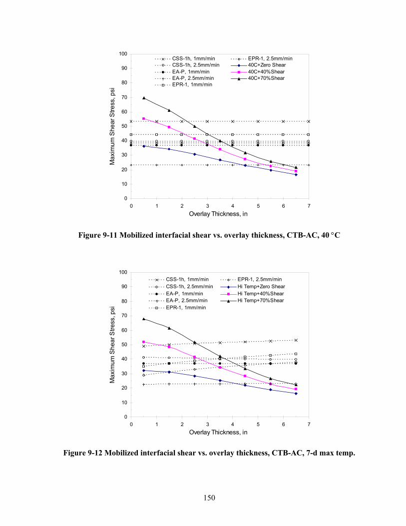
150
0
10
20
30
40
50
60
70
80
90
100
0 1 2 3 4 5 6 7Overlay Thickness, in
Max
imum
She
ar S
tress
, psi
CSS-1h, 1mm/min EPR-1, 2.5mm/minCSS-1h, 2.5mm/min 40C+Zero ShearEA-P, 1mm/min 40C+40%ShearEA-P, 2.5mm/min 40C+70%ShearEPR-1, 1mm/min
Figure 9-11 Mobilized interfacial shear vs. overlay thickness, CTB-AC, 40 °C
0
10
20
30
40
50
60
70
80
90
100
0 1 2 3 4 5 6 7Overlay Thickness, in
Max
imum
She
ar S
tress
, psi
CSS-1h, 1mm/min EPR-1, 2.5mm/minCSS-1h, 2.5mm/min Hi Temp+Zero ShearEA-P, 1mm/min Hi Temp+40%ShearEA-P, 2.5mm/min Hi Temp+70%ShearEPR-1, 1mm/min
Figure 9-12 Mobilized interfacial shear vs. overlay thickness, CTB-AC, 7-d max temp.

151
10 Summary, Conclusions and Recommendations
10.1 Summary and Conclusions
This study investigated the causes(s) of excessive delamination and shoving distress
observed in NCDOT Division 13. Two potential causes of these distresses were identified to
be: (a.) Unstable mixtures caused due to intermittent purging of baghouse fines, and, (b.)
Improper choice and/or application of tack coat.
Work conducted by Tayebali et al [28] evaluated the field cores and their compliance
with NCDOT specifications. The field cores were obtained based on a survey conducted in
Division 13 of NCDOT. Field cores from two counties, Buncombe and Rutherford, were
selected for evaluation. The results of gradation, volumetric, and stability analysis indicated
that the in-situ asphalt mixes used in Buncombe and Rutherford counties were generally
within the NCDOT design specifications, and should have performed well under normal
traffic conditions. Buncombe County sections, however, had excessive delamination and
shoving distresses whereas Rutherford County sections did not show an occurrence of any of
such distresses. It was originally hypothesized that one of the contributory factors to the
delamination and shoving was the intermittent purging of baghouse fines in the field asphalt
mixtures and, therefore, additional laboratory tests were conducted to verify the claim.
Gradation analysis using particle analyzer, however, showed comparable gradations for
baghouses and regular mineral fillers for both counties. The dynamic mechanical analysis of
mastics using DSR suggested that baghouse fines might lead to stiffening of the binders, and
consequently increased rut resistance of AC mixes. Further, there was no significant
difference in |G*| values of mastics prepared with baghouses versus regular filler. Laboratory
FSCH and RSCH tests conducted on mixes with baghouse fines showed that:
• Baghouse fines have a stiffening on mixes from both counties;
• Mixes containing baghouse fines are more resistant to rutting compared to mixtures
without baghouse fines; and
• Mixes from both counties show similar dynamic shear stiffness and rutting
characteristics.
152
Mixtures containing regular mineral filler and baghouse fines were subjected to APA
testing at NCDOT Materials and Test Unit. Test results showed that the accumulated rut
depths for mixtures from Buncombe and Rutherford counties were approximately 6.15-mm
(1/4-inch) and 12.5-mm (1/2-inch), respectively, for both mixtures with and without
baghouse fines. Although, these rut depths suggest excessive rutting susceptibility for mixes
based on the NCDOT specification, it confirms findings based on other tests that indicated
that the performance of mixtures with and without baghouse fines are very similar. However,
the modified AASHTO T283 test clearly indicated that the mixtures containing baghouse
fines were moisture sensitive as compared to the mixtures containing regular mineral filler
even though, an anti-strip additive was used for both mixtures. The TSR ratios for the
Buncombe County mixtures were 78 and 85-percent for mixtures with and without baghouse
fines, respectively. The TSR ratios for Rutherford County mixtures were 83 and 92-percent
for mixtures with and without baghouse fines, respectively.
Based on the results of this investigation, it is concluded that the intermittent purging
of baghouse fines could be the contributory factor in the delamination and shoving distress
observed in NCDOT Division 13. It appears that the mechanism by which this distress is
manifested is the following:
• Some in-situ mixtures may contain very high proportion of baghouse fines in relation to
regular fines due to intermittent purging of the baghouse fines. Although the NCDOT
JMF requires use of an anti-strip additive, the dosage does not appear to be sufficient to
counter act moisture damage leading to in-situ mixture deterioration and, consequently,
loss of strength and stability. Once the moisture damaged mixture is susceptible to
shoving under traffic loading, the CRS-2 emulsion is not able to provide the tacking
strength necessary for the surface layer to remain bonded to the lower layer, hence,
leading to delamination.
• In Rutherford County where some pavement sections may contain relatively higher
amount of baghouse fines due to intermittent purging, the PG64-22 binder used as tack
coat appeared to provide sufficient bonding that may prevent asphalt layer from
delaminating even though mixtures may undergo slight moisture damage.

153
Apart from intermittently purging baghouse fines into mixes, the pavement sections in
Rutherford and Buncombe counties use CRS-2 emulsion and PG64-22 binder as tack coat.
The improper use of tack coat could be a contributory factor to delamination distresses
observed in those counties. It was, therefore, decided to investigate the contribution of prime
and tack coat bond strength contribution to the integrity of pavements in relation to overlay
AC thickness. The goal was to develop a mechanistic design procedure to minimize the
occurrence of delamination distresses.
A survey was conducted across all the state highway departments and agencies to
acquire information about the use of prime and tack coats in the field. Of the 26 responding
agencies, ten reported that there was no requirement on use of prime coat for new
construction. A majority of the remaining sixteen used a combination of cutbacks and
emulsions for prime coats. Only two states, Georgia and New Jersey, require use of prime
coat if the AC thickness is less than 5 inches, and Missouri requires it if the AC thickness is
less than 4 inches. For prime and tack coats, there was no objective test to ensure proper
curing. This could, potentially, lead to a lot of problems during the service life.
DSR test results on residual binders from emulsions were used to determine their PG
grade. Generally, with higher the PG rating greater would be the expected shear strength.
Using rolling wheel compaction, composite AC-AC, and PCC-AC specimens were fabricated
in the lab. The target air void content for all AC specimens was 4%. Problems encountered in
fabricating CTB slabs, required CTB-AC composite fabrication in gyratory molds. Before
paving the overlay, the lower layer was tacked or primed, and the emulsions were allowed to
cure for 24 hours. The rate of application was 0.06 and 0.24 gallons per square yard for tack
coat and prime coat, respectively. The samples were then cored and cut to 6-inch diameter
and 2-inch height before being tested in simple shear at various temperatures.
A displacement rate of 1.0 and 2.5 mm per minute was used to determine the bond
strength of the specimens. The test results concluded that:
• Non-bonded surfaces have extremely low strengths compared to bonded surfaces.
Therefore, use of a bonding agent (tack or prime coat) is always recommended during
constructions.

154
• For AC-AC composites, the performance of PG64-22 binder as a tack coat is better than
CMS-2 emulsion. This is supported by higher axial and shear strengths of PG64-22
tacked specimens compared to CMS-2 specimens.
• For PCC-AC specimens, the behavior of PG64-22 as tack coat is comparable to CMS-2.
One reason for this could be due to the fact that the rate of application of residual
asphalt could be higher for PG64-22 than for CMS-2. In particular, it was found that
PG64-22 performance at higher temperature and lower strain rate was relatively poor.
The bond strengths recorded for PCC-AC combination were substantially lower
compared to AC-AC. Secondly; the relative imperviousness of PCC (vis-à-vis AC)
could lead to less absorption of asphalt from tack coat and, consequently, a poorer
bond at high temperature and low strain rate. The relative differences in PCC and AC
moduli could also be a contributory factor as well as the absence of corrugations on the
PCC slab. In the field, the underlying concrete pavement has grooves or milled surface
that increases the friction between the overlay and the PCC slab.
• The bond development in CTB-AC case was due to a contribution of the prime coat as
well as aggregate interlock. CSS-1h emulsion performed better than EA-P and EPR-1
emulsions as prime coat.
Using shear and axial frequency sweep tests, the dynamic moduli of asphalt mix were
determined at various temperatures and, properties for PCC were determined at 28 days.
Based on the pavement temperature at various depths, the dynamic moduli and interfacial
bond strengths were interpolated to yield temperature-corrected values. These values
(dynamic moduli) coupled with the standard 18-kip loading data were, then, input into the
FLA program developed in this investigation. The program computed the stresses, strains and
displacements at various points in the pavement structure as function of vertical as well as
horizontal shear loading. The maximum shear stresses were computed at the interface for
different loading conditions. The variation of maximum mobilized shear stresses was then
plotted against the interpolated bond strengths to obtain the required minimum design
thicknesses.
For AC-AC, at 7-day maximum average temperatures, the overlay design thickness
using CMS-2 and PG64-22 tack coat and shear displacement rate of 1.0 mm/minute was

155
comparable (3.5 inch); however at 2.5 mm/minute displacement rate PG64-22 (2.5 inch)
gave a lower design thickness than CMS-2 (3.25 inch) indicating a superior performance.
Mechanistic analysis indicates that delamination will not be a problem for AC-AC
combination at 20 °C as the bond strengths are much higher than the mobilized interfacial
shear stresses. For PCC-AC combination, at 20 °C and 2.5 mm/minute displacement rate, the
design thickness for AC overlay is slightly higher than 2-inch; at the same temperature and
1.0 mm/minute the design thickness for CMS-2 and PG64-22 is 2.5 and 4 inch, respectively.
Therefore, it can be concluded that CMS-2 yields lower thickness for PCC-AC combination
than PG64-22 binder. As indicated earlier, this could be due to excess PG64-22 (compared to
the residual asphalt in CMS-2), smooth PCC surface, and low rate of tack coat absorption by
the PCC surface. At 7-day maximum temperature, for PCC-AC combination, the interpolated
bond strengths are much lower than the mobilized shear stresses. Therefore, the choice of
tack coats is dependent not only on the types of interfaces under consideration but also on the
rate of application. Higher rate of tack coat is undesirable when using impervious and smooth
surfaces as PCC. At higher temperature, instead of providing a good bond, it will actually act
as a slippage surface. In severe cases it may even lead to bleeding on the thin AC overlay
layer.
For CTB-AC interface, CSS-1h emulsion seems to be better than EA-P and EPR-1.
Overall, based on the results of this study, the following conclusions can be drawn:
• Addition of baghouse fines could cause stiffening of AC mixes. However, appropriate
amounts of anti-strip additive needs to be added to counteract the added moisture
susceptibility due to the presence of baghouse fines.
• The contribution of tack coat to the bond strength is dependent on the grade of the
residual asphalt as well as the interfaces under consideration. PG64-22 performs
slightly better for the AC-AC case whereas CMS-2 performs marginally better for
PCC-AC case.
• For thin pavement sections, the use of prime coats is recommended to increase the bond
between the AC layer and the underlying layers. Similarly, use of a suitable tack coat is
recommended for all overlay construction with minimum AC layer thickness of 2.5-3.5
inches when PG64-22 or CMS-2 emulsion is used as tack coat. If a different tack coat

156
is used, the minimum thickness can be obtained for the given site using the design
guidelines developed in this study.
• CSS-1h performs better as a prime coat than EA-P and EPR-1 emulsions.
• For emulsions used as prime and tack coats, it is necessary to ensure complete curing
before paving new layer. Any inappropriate curing could reduce the bond as well as
trap moisture causing problems later in service.
• The choice of proper tack coat (CMS-2 versus PG64-22) should be based on operational
considerations. Use of PG64-22 as tack coat enables the tacked section to be open to
traffic immediately after application. Further the convenience of night time paving as
well as minor effect on exposure moisture outweighs the trouble of dealing with hot
asphalt. Curing problems with emulsions prevail over the uniformity and ease of their
application.
Finally, this research study provides a methodology and design guide based on mechanistic
analysis to select appropriate tack or prime coat for the given field conditions. Based on
selection of the tack or prime coat, the AC layer thickness can be adjusted to minimize the
delamination distresses.
10.2 Future Scope
The study conducted herein compared the bond strengths of various materials at 1.0
and 2.5 mm/minute shear displacement rate. Following aspects need to be examined further:
• The current results should be validated by testing laboratory fabricated composite slabs
under wheel-tracking device, and field testing.
• The current study is based on laboratory tests, testing of the field cores from various
pavement sections (good performing vs. poor performing) should be explored to get a
correlation between the laboratory test results and field observations.
• Laboratory testing could be conducted under multi-axial loading states to simulate in-situ
condition closely.

157
• The various loading conditions used for analysis use a static load. A relationship needs to
be developed between the following:
o Vehicular speed and the rate of shear strain as function of depth, and
o Vehicular speed and loading frequency.
• The analyses conducted using the FLA program assume isotropy, elastic behavior, and
homogeneity. Approaches that consider anisotropy and viscoelastic behavior could
offer significant insight into the complex behavior of asphalt materials.
.

158
11 References 1. American Association of State Highway and Transportation Officials, “AASHTO
Guide for Design of Pavement Structures,” pp. II-23, 1993.
2. American Association of State Highway and Transportation Officials, “Standard
Specification for Performance Graded Asphalt Binder,” AASHTO Designation MP1,
1996.
3. American Association of State Highway and Transportation Officials, “Standard
Method for Preparing and Determining the Density of Hot Mix Asphalt (HMA)
Specimens by Means of the SHRP Gyratory Compactor,” AASHTO Designation TP4,
1996.
4. American Association of State Highway and Transportation Officials, “Standard Test
Method for Determining the Rheological Properties of Asphalt Binder Using a
Dynamic Shear Rheometer (DSR),” AASHTO Designation TP5, 1996.
5. American Association of State Highway and Transportation Officials, “Standard Test
Method for Determining the Permanent Deformation and Fatigue Cracking
Characteristics of Hot Mix Asphalt using a Simple Shear Test Device,” AASHTO
Designation TP7, 1996.
6. Ameri-Gaznon, M., and Little, D., “Octahedral Shear Stress Analyses on an ACP
Overlay on a Rigid Base,” Proceedings of the Association of Asphalt Paving
Technologists, vol. 59, pp. 443-479, 1990.
7. Asphalt Institute, “Asphalt in Pavement Maintenance,” Manual Series No. 16 (MS-
16), Third Edition, 1996.
8. Barber, E. S., “Shear Loads on Pavements,” Public Roads, vol. 32, no. 6, pp. 141-
144, 1963.
9. Bonnaure, F., Gavois, A., and Udron, J., “A New Method for Predicting the Fatigue
Life of Bituminous Mixes,” Proceedings of the Association of Asphalt Paving
Technologists, vol. 49, pp. 499-529, 1980.

159
10. Burmister, D. M., “The General Theory of Stresses and Displacements in Layered
Systems,” Journal of Applied Physics, vol. 16, pp. 89-94, 126-127, 296-302, February
1945.
11. Epps, J. A., and Button, J. W., “The Slippage Question on Airport Pavements,” Texas
Transportation Institute, Interim Report, RF3424-2.
12. Hachiya, Y., and Sato, K., “Effect of Tack Coat on Bonding Characteristics at
Interface between Asphalt Concrete Layers,” Proceedings of 8th International
Conference on Asphalt Pavements, vol. 1, pp. 349-362, 1997.
13. Harris, B. M., and Stuart, K. D., “Analysis of Mineral Fillers and Mastics used in
Stone Matrix,” Proceedings of the Association of Asphalt Paving Technologists, vol.
64, pp. 54-95, 1995.
14. Huang, Y. H., “Pavement Analysis and Design,” Pearson Prentice Hall, second
edition, 2004.
15. Ishai, I., and Livneh, M., “Functional and Structural Role of Prime Coat in Asphalt
Pavement Structures,” Proceedings of the Association of Asphalt Paving
Technologists, vol. 53, pp. 98-118, 1984.
16. Kummer, H. W., and Meyer, W. E., “Tentative Skid-Resistance Requirements for
Main Rural Highways,” NCHRP Report 37, Highway Research Board, 1967.
17. Metcalf, J. B., “Accelerated Pavement Testing, a Brief Review Directed Towards
Asphalt Interests,” Proceedings of the Association of Asphalt Paving Technologists,
vol. 67, pp. 553-572, 1998.
18. Mohammad, L. N., Raqib, M. A., and Huang, B., “Influence of Asphalt Tack Coat
Materials on Interface Shear Strength,” Transportation Research Record, no 1789,
pp. 56-65, 2002.
19. Mukhtar, M. T., and Dempsey, B. J., “Interlayer Stress Absorbing Composite (ISAC)
for Mitigating Reflection Cracking in Asphalt Concrete Overlays,” Final Report
Project IHR-533, Illinois Cooperative Highway Research Program, June, 1996.

160
20. Paul, H. R., and Scherocman, J. A., “Friction Testing of Tack Coat Surfaces,”
Transportation Research Record, no. 1616, pp. 6-12, 1998.
21. Shahin, M. Y., Kirchner, K., Blackmon, E.W., and Tomita, H., “Effect of Layer
Slippage on Performance of Asphalt-Concrete Pavements,” Transportation Research
Record, no. 1095, pp. 79-85, 1986.
22. “SHRP Superpave Binder Selection Program – SHRPBIND,” version 2.1, Federal
Highway Administration, Pavement Performance Division, McLean, Virginia, 1985.
23. “SHRP-A-415 Permanent Deformation of Asphalt Aggregate Mixes,” Strategic
Highway Research Program, National Research Council, Washington DC, 1994.
24. Sholar, G. A., Page, G. C., Musselman, J. A., Upshaw, P. B., Moseley, H. L.,
“Preliminary Investigation of a Test Method to Evaluate Bond Strength of
Bituminous Tack Coats,” Proceedings of the Association of Asphalt Paving
Technologists, Preprints, pp. 107-137, 2004.
25. Small, J. C., and Booker, J. R., “Finite Layer Analysis of Layered Elastic Materials
Using a Flexibility Approach. Part 1 – Strip Loadings,” International Journal for
Numerical Methods in Engineering, vol. 20, pp. 1025-1037, 1984.
26. Small, J. C., and Booker, J. R., “Finite Layer Analysis of Layered Elastic Materials
Using a Flexibility Approach. Part 2 – Circular and Rectangular Loadings,”
International Journal for Numerical Methods in Engineering, vol. 23, pp. 959-978,
1986.
27. Tayebali, A. A., Fischer, W. K., Huang, Y. X., and Kulkarni, M. B., “Effect of
Percentage Baghouse Fines on the Amount and Type of Anti-Stripping Agent Required
to Control Moisture Sensitivity,” Final Report, North Carolina Department of
Transportation, June 2003.
28. Tayebali, A. A., Kulkarni, M. B., and Waller, H. F., “Delamination and Shoving of
Asphalt Concrete Layers Containing Baghouse Fines,” North Carolina Department of
Transportation Project 1999-03, FHWA/NC/2002-011, May 2000.

161
29. Tschegg, E., Kroer, G., Tan, D., Stanzl-Tschegg, S., and Litzka, J., “Investigation of
Bonding between Asphalt Layers on Road Construction,” Journal of Transportation
Engineering, vol. 121, no. 4, pp. 309-316, 1995.
30. Uzan, J., “Influence of the Interface Condition on Stress Distribution in a Layered
System,” Transportation Research Record, no. 616, pp. 71-73, 1976.
31. Uzan, J., Livneh, M., and Eshed, Y., “Investigation of Adhesion Properties between
Asphaltic-Concrete Layers,” Proceedings of the Association of Asphalt Paving
Technologists, vol. 47, pp. 495-521, 1978.
32. Xu, Q., Rahman, M. S., and Tayebali, A. A., “FLA: A Computer Program for Finite
Layer Analysis of Stresses in Pavements,” Department of Civil Engineering, North
Carolina State University, June 2002.

162
Appendix A
Questionnaire – ON PRIME AND TACK COATS
A Mechanistic Approach to Evaluate Contribution of Prime and Tack Coat
In Composite Asphalt Pavements
North Carolina Department of Transportation, Project HWY-2001-04
Scope of the Survey: An evaluation of the effectiveness of emulsified asphalt prime coats as compared to cutback asphalt prime coats, and to make a survey of the state practices with respect to types and rates of application of both prime coats and tack coats.
Responding Agency:
Name and Title of Individual Completing Questionnaire:
Does your agency require the use of a prime coat on new construction?
Yes ___ NO ____
If the answer to question 1 is yes, what are the required type of material and the normal rate of application? ____________________________________________________________________
Is the use of prime coat related to asphalt pavement thickness? If so, explain
Is a specific cure time specified? Yes ___ No ____
If yes, how much cure time? _____________________________________________
What types of laboratory tests are required for prime coat material(s) ?

163
Are any types of field performance test(s) required? Yes ___ NO ___. If yes, please explain ______________________________________________________________
Have you been able to detect any difference in pavement performance by using or not using a prime coat? Yes ___ No ___. If yes, please explain _____________________
Do you have opinion as to the merits of an emulsified asphalt prime as compared to a cutback asphalt prime? Yes ____ NO ___. If yes, please explain ________________
What types of asphalt materials are used for tack coats – types and application rates?
If you use emulsified asphalt tack coats for nighttime paving, what provisions are made for the emulsion breaking prior to placement of the hot-mix asphalt?
Please return completed questionnaire to:
Prof. Akhtar A. Tayebali, P.E.
North Carolina State University
Department of Civil Engineering
Campus Box 7908
Raleigh, NC 27695-7908
Ph: (919) 515-7611
Completed questionnaires can be faxed at (919) 515-7908. If you prefer to fill this questionnaire in electronic format, please send an e-mail to [email protected].
164
Appendix B
Stat
e
Prim
e C
oat
Prime Coat Materials
PC R
ate
(gal
/yd2 )
PC relation to AC thickness
Cur
e Ti
me
How
muc
h?
Lab Tests for Prime Coats
Fiel
d PT
?
Fiel
d Pe
rfor
man
ce
Test
D
escr
iptio
n
Diff
. in
perf
.?
Explanation
Explanation: why emulsion is better than
cutback or vice versa.
Tack Coat Types
Tack
Coa
t R
ates
(g
al/y
d2 )
Night time provisions
AK Y/N
MC-30 or CSS-1
250-750 ml/sq. m
N, The application of tack coat is dependent on individual designers and on the paving location.
N
MC-30 must meet M82. CSS-1 must meet M140.
N N -
Y, Cutbacks penetrate better than the emulsified asphalts.
Special Tack Emulsion -1
200-400 ml/sq.m
Tack coat may not be placed on a wet surface or when the roadway surface temp is below 5 deg. C.
AL Y
AE-P, MC-30, MC-70 for tight bases. MC-250, MC 70, RC-250 for open bases, EPR
0.22 - 0.25 20% redn. for CTB
No N M81, M82, spot test is not required.
N Y
Protects base from wind/water erosion and promotes the maintenance of optimum m/c by creating an impermeable membrane.
Better penetration and better coverage from cutback asphalt.
CRS-2, CRS-2h, CSS-1, CSS-1h, CSQ-1hp, PG 67-22
As directed by engr but < 0.07
Eliminating the use of emulsified asphalt tack coats because it is not possible to determine whether emulsion has broken or not.
AR N MC cutbacks 0.4
N, Except for a minimum thickness of hot mix on minor roadways.
Y 3 days
Distillation, softening point, penetration, viscosity, spot test.
N N - - RC cutbacks, emulsions
0.03 - 0.10
Observation of the inspector.
AZ N - - - - - Kinematic Viscosity N N -
N, MC-250 is the only thing used in AZ.
AC, SS-1
AC @ 0.06, SS-1 & ERA-25 -1:1 dilute w/ water @ 0.08
Nothing specified. Emulsion must break before paving of AC.
CT Y Emulsions. 0.14-0.45 liter/sq. m
No, but prime coats are required only on airports.
Y Tacky to touch.
Percent residue, viscosity..
N N - - SS-1, SS-1H
0.14-0.45 liter/sq. m
None.

165
St
ate
Prim
e C
oat
Prime Coat Materials
PC R
ate
(gal
/yd2 )
PC relation to AC thickness
Cur
e Ti
me
How
muc
h?
Lab Tests for Prime Coats
Fiel
d PT
?
Fiel
d Pe
rfor
man
ce
Test
D
escr
iptio
n
Diff
. in
perf
.?
Explanation
Explanation: why emulsion is better than
cutback or vice versa.
Tack Coat Types
Tack
Coa
t R
ates
(g
al/y
d2 )
Nig
ht ti
me
prov
isio
ns
FL Y
RC-70, RC-250. SS-1, CSS-1, SS-1H diluted. AE-60, AE-90, AE-150, AE-200, Sp. MS-Emulsion diluted at a ratio of six parts of emulsion to four parts of water. AEP, EP (RS type), EPR-1 Prime.
> 0.1 N N Sec. 916-3 and 916-4 of FDOT. N - Y
Prime is thought to act as a barrier to moisture to frequent rains in Florida. Better bond between AC and base course. Also acts as barrier for moisture when penetration happens through cracks.
- - - -
GA Y RC-30, RC-70, MC-30, MC-70, EAP-1
0.7 - 1.4 liters/sq. m
PC required on all soil-cement and lime stabilized bases and on all other bases unless AC > 125 mm
N
T55, T79, T48, T201, T78, T51, T44, T49, T50, T72, T111
N - - - - PG 58-22, PG64-22, PG67-22
0.18 - 0.27 liters / sq. m
N/A
ID N MC-70, MC-250, CSS-1 0.3
No, related more to the amount of traffic on the base. Helps when thin lifts of asphalt are present
N M82 - cutbacks T59 - emulsions N
PC matl. Accepted by certification. Verification samples taken; may or may not be tested.
Y
Thinner pavements (0,2') shove and tear on grades and in curves where prime is not used.
Cutbacks penetrate better but environmental problems.
Diluted CSS-1 0.05 None at
this time.
IL Y RC-70 0.02
Only on full depth pavements is prime coat required. N
Y
Min
. 1 h
our.
Sp. Gr, Kin. Visc., Distillation, Test on residue, penetration, ductility, % soluble in TCE
N - N
Considered paving without in late 1997. Cost savings considered minimal and not worth the risk.
We allow emulsions for resurfacing projects - with success.
resurfacing: SS-1, SS-1H, CSS-1, CSS-1H, HFE60, HFE90, RC-70
0.05-0.1 Just emulsion breaking.
KS N - - Not used. - - - - - - - Emulsions do not penetrate.
CSS-1H, SS-1H diluted 50%
0.03-0.05
Must break down before overlay.

166
St
ate
Prim
e C
oat
Prime Coat Materials
PC R
ate
(gal
/yd2 )
PC relation to AC thickness
Cur
e Ti
me
How
muc
h?
Lab Tests for Prime Coats
Fiel
d PT
?
Fiel
d Pe
rfor
man
ce
Test
D
escr
iptio
n
Diff
. in
perf
.?
Explanation
Explanation: why
emulsion is better than cutback or vice versa.
Tack
Coa
t Ty
pes
Tack
Coa
t R
ates
(g
al/y
d2 )
Night time provisions
KY Y Primer-L: cutback asphalt emulsion.
1.6-2.0 lb/sq. yd No Y
"mus
t cur
e!"
Saybolt Furol, Water Content, Asphalt Content, Coating, Residue Test Float, Solubility in Tri-chloro-ethylene
Y
Sampling of Primer_L @ 1 per 15000 tons of AC and the same tests.
N -
Cutbacks perform better as sealants but concern about health and environment.
SS-1, SS-1H, CSS-1, CSS-1h, AE-60, RS-1, CRS-1
0.4 lb/sq. yd
It is necessary to have all water to be evaporated before any paving process.
ME N -
0.02 for overlays, 0.04 for milled and 0.01 for new mixes tacked at Contractors option
N, Tack coat is not needed for new construction only on overlaid pavement's or lower layers that have been exposed to winter or have got dirty.
N -
M140 Ductility, Penetration, Sieve test for lumps, Oil content, Float test, Viscosity at 25 deg. C.
N - Y
Contractors find easy to densify SUPERPAVE mixes. QA bonus makes up for the cost of the tack. Less delamination and when applied properly it is impossible to separate tacked layers in cores without a saw.
N
Emulsions and are required only when overlaying an old pavement that is dirty or has wintered over.
-
Little night time paving but breaking can be decided in artificial lights.
MN N
Although the specifications exist in the "handbook" Prime Coat is not used in practice. MC-30, MC-70.
0.45-1.35 liter/sq. m - - - - - - - N
MC-250, MC-800, C-70, C-250, C-800, SS-1, SS-1H, MS-2, RS-1, RS-2, CSS-1, CSS-1H, CRS-1, CRS-2
0.23 lit/sq.m for cutbacks and undiluted emulsions. 0.91 lit/sq.m for diluted emulsions. Water may be added upto 0% for SS-1, SS-1H, CSS-1 and CSS-1H.
Currently requiring the emulsion to break completely.

167
Stat
e
Prim
e C
oat
Prime Coat Materials
PC R
ate
(gal
/yd2 )
PC relation to AC thickness
Cur
e Ti
me
How
muc
h?
Lab Tests for Prime
Coats
Fiel
d PT
?
Fiel
d Pe
rfor
man
ce
Test
D
escr
iptio
n
Diff
. in
perf
.?
Explanation
Explanation: why emulsion is better than
cutback or vice versa.
Tack Coat Types
Tack
Coa
t R
ates
(g
al/y
d2 )
Night time provisions
MO Y RC-70, MC-30 or SS-1 0.2-0.5
Primer not used for plant mix bituminous base with a thickness of 4" or more.
N - M81, M82 or M140 N - N We have always required
the use of prime coat.
Y, Emulsions have more pickup versus cutback.
SS-1, SS-1H, CSS-1, CSS-1H 0.
02-0
.1 No provisions
for emulsion tack coats during night time paving.
MS Y
CTB - MC-70, EA-1. Lime treated: EA-1, SS-1, CSS-1, CMS-2h, MS-2h
CTB-0.1-0.25. Lime: 0.25
N N - T59, M82, M140, M208
N - Y
Indirectly, we know that unprimed chemically stabilized courses do suffer moisture damage, but it could be related as much to the stabilization effort as it is to the prime coat.
Y, emulsions are easier for contractors to use and work well when applied properly.
SS-1, CSS-1 and some AC-30
- -
NE N - - - - - - - - N - Y, Environmental Issue.
CSS-1H when diluted with water to reduce AC content to 30% of total vol.
0.1-
0.2
on e
xist
ing
or
mill
ed s
urfa
ces.
OR
0.
05-0
.1 o
n fre
shly
laid
A
C.
Required to be broken before placement. But it is not always the case. We have not discovered any problems when unbroken tack was covered with hot mix.
NH N PC not required since 1974. N N RS-1, CRS-1
0.025
Emulsion breaking should be very quick.
NJ Y MC-30, MC-70
0.68-1.58 liter/sq. m
The engineer may waive the application of prime coat if a minimum of 125 mm of plant AC mix is placed on unbound aggregate course prior to opening to traffic.
N - M82 Y
No volatile organic substances under normal use conditions.
N
Currently attempting to eliminate the prime coat requirement. More often eliminated than not on projects.
-
RC-70, RC-T, RS-1, SS-1, SS-1h, CSS-1, CSS-1h. Emulsion used determined by Calendar.
See sec. 404.13 Tacky to touch.
168
Stat
e
Prim
e C
oat
Prime Coat Materials
PC R
ate
(gal
/yd2 )
PC re
latio
n to
AC
th
ickn
ess
Cur
e Ti
me
How much?
Lab Tests for Prime Coats
Fiel
d PT
?
Fiel
d Pe
rfor
man
ce
Test
D
escr
iptio
n
Diff
. in
perf
.?
Explanation
Explanation: why emulsion is better than
cutback or vice versa.
Tack Coat Types
Tack
Coa
t R
ates
(g
al/y
d2 )
Nig
ht ti
me
prov
isio
ns
NY N - - - - - - - - - - - HFMS-2h, SS-1h, CSS-1h
diluted application rate: 0.14-0.32 lit./sq. m
Currently under discussion.
OK Y/N
MC-30, MC-70 or emulsions in Oklahoma, Tulsa and Commanche Counties
0.1-
0.4
N N
Sufficient to allow proper penetration and hardening of prime coat.
Kinematic Viscosity @140 C, Flash Point, % Water, Distillation, Abs Viscosity, Ductility, Solubility in Trichloroethylene, Spot Test.
Y/N
No performance tests but lab tests, viscosity (140), Distillation.
Y
We had one project this year that had significant plane slippage problems due to use of tack coats in lieu of prime coat.
Y, Emulsions to be used where environment is a concern and also if conditions warrant and wherever there is sufficient time for curing.
RS-1, RS-2, MS-1, MS-2, MS-2h, HFMS-1, HFMS-2, HFMS-2h, HFMS-2s, SS-1, SS-1h, CRS-1, CRS-2, CMS-1, CMS-2, CSS-1, CSS-1h
0.1 Emulsions disallowed after sunset.
RI N - - - - - - - - - - - SS-1 0.05
Emulsions used for night time paving but no provisions exist for breaking prior to placement.
SC Y -
0.25
-0.3
N N - Saybolt Furol, Residue by Distillation.
N - N - N CRS-2, HFMS-1
0.05-0.15 based on residual asphalt.
None, contractors electing to use RS emulsion if needed.
TN Y AE-P, CAE-P 0.
2-0.
5
N N -
M140, Saybolt Furol, Settlement, Residue, Distillate, Float, Penetration, Solubility.
N - N - N SS-1, CSS-1, PG64-22
0.05 for smooth (max.) and 0.2 (max) for milled.
None
169
Stat
e
Prim
e C
oat
Prime Coat
Materials PC R
ate
(gal
/yd2 )
PC relation to AC thickness
Cur
e Ti
me
How
muc
h?
Lab Tests for Prime Coats
Fiel
d PT
?
Fiel
d Pe
rfor
man
ce
Test
D
escr
iptio
n
Diff
. in
perf
.?
Explanation
Explanation: why emulsion is better than
cutback or vice versa.
Tack Coat Types
Tack
Coa
t R
ates
(g
al/y
d2 )
Night time provisions
TX Y
MC-30, AEP, PCE, EAP&T. CSS-1 and SS-1
0.1
Emulsions can be used but have to be worked into the top inch and recompacted.
N - Item 300 of "Asphalts, Oils and Emulsions." N
For new materials, testing is required.
N
Compulsory, therefore nothing to compare with.
Y, MC-30 penetrates best. For open bases, emulsion may be good.
diluted SS-1, CSS-1 0.05
Not aware of any special considerations.
WV Y
SS-1, SS-1h, CSS-1, CSS-1h diluted with water. Inverted emulsions permitted but rarely used.
0.3 - 0.6 N N - M140, M208 N - N -
Cutbacks penetrate better but environmental problems and costly.
Mostly SS emulsions (cationic, anionic, inverted)
0.2 - 0.3; SS-1h diluted with 50% water is commonly used.
No special requirements.
WY Y MC-70 3.2 lb/sq yd No N -
M82, Kinematic viscosity, distillation. Have an acceptance schedule based on properties.
N - Y
We feel the prime facilitates placing the first lift of pavement and also provides some water proofing.
N SS-1 or CSS-1
0.25 lb/sq yd
Do very little night time paving.

170
Appendix C
Job Mix Formula

171
99410 NORTH CAROLINA DEPARTMENT OF TRANSPORTATION
RALEIGH, NORTH CAROLINA 27611
HOT MIX ASPHALT JOB MIX FORMULA APAC-CAROLINA, INC TYPE MIX: BCSC, TYPE HDS
ENKA, NC JOB MIX FORM NO: 93-447-052
EFFECTIVE DATE: 07-27-93
PLANT CERTIFICATION NO: DM-310 PROJECT NO:
COUNTY: BUNCOMBE
AGGREGATE SOURCES AND BLEND PERCENTAGES SUPPLIER LOCATION/SOURCE MATERIAL BLEND(%)
VULCAN MATERIALS ENKA QUARRY #78M 42 VULCAN MATERIALS ENKA QUARRY W.SCRGS. 30 VULCAN MATERIALS ENKA QUARRY D.SCRGS. 28
TOTAL: 100.0% JMF COMBINED GRADATION ASPHALT CEMENT %(TOT) 5.7 SIEVE SIZE % PASSING 2’’ GRADE PG64-22 1 ½ ’’ EST ASH 11-3-93 0.3 1’’ MAX. SP. GV. 2.486 ¾’’ 100 LABORATORY SP. GV. 2.364 ½’’ 98 VOIDS IN TOTAL MIX % 4.9 3/8’’ 95 MIN. % COMPACTION 95.0 NO. 4 72 MIX TEMPERATURE F. 285 8 50 FLOW (0.01 IN.) 11 16 39 STABILITY (LBS.) 3000 40 24 NON STRIP ADDITIVE % 0.50 80 12 MODIFIER % 0.00 200 5.0 ASPHALT CEMENT SUPPLIER : SPECS. TACK COAT SUPPLIER : SPECS. NON-STRIP ADD. SUPPLIER : PAVE BOND LP – CINCINNATI, OHIO MODIFIER SUPPLIER : COMMENTS:
% AC DECREASED TO INCREASE VOIDS. BLEND CHANGES TO CONTROL GRADATION & VOIDS IN MIX. #8 SIEVE CHANGE BASED ON FIELD TEST RESULTS.
DATE JMF VOID:
APPROVED BY: J.E. GRADY, JR.
PAVEMENT CONSTRUCTION ENGR.

172
99410 NORTH CAROLINA DEPARTMENT OF TRANSPORTATION
RALEIGH, NORTH CAROLINA 27611
HOT MIX ASPHALT JOB MIX FORMULA THOMPSON CONTRACTORS, INC TYPE MIX: BCSC, TYPE HDS
RUTHERFORDTON, NC JOB MIX FORM NO: 93-903-051
EFFECTIVE DATE: 02-07-94
PLANT CERTIFICATION NO: DM-286 PROJECT NO:
COUNTY: RUTHERFORD
AGGREGATE SOURCES AND BLEND PERCENTAGES SUPPLIER LOCATION/SOURCE MATERIAL BLEND(%)
THOMPSON CONTRACTORS MILLER CREEK QUARRY #78M 47 THOMPSON CONTRACTORS MILLER CREEK QUARRY SCRGS. 33 THOMPSON CONTRACTORS BROAD RIVER SAND 20
TOTAL: 100.0% JMF COMBINED GRADATION ASPHALT CEMENT %(TOT) 6.2 SIEVE SIZE % PASSING 2’’ GRADE PG64-22 1 ½ ’’ EST ASH 11-3-93 0.4 1’’ MAX. SP. GV. 2.502 ¾’’ 100 LABORATORY SP. GV. 2.378 ½’’ 98 VOIDS IN TOTAL MIX % 5.0 3/8’’ 95 MIN. % COMPACTION 95.0 NO. 4 69 MIX TEMPERATURE F. 285 8 53 FLOW (0.01 IN.) 9 16 43 STABILITY (LBS.) 1900 40 24 NON STRIP ADDITIVE % 0.50 80 11 MODIFIER % 0.00 200 5.9 ASPHALT CEMENT SUPPLIER : SPECS. TACK COAT SUPPLIER : SPECS. NON-STRIP ADD. SUPPLIER : PERMA-TAC — SCAN ROAD MODIFIER SUPPLIER : COMMENTS:
DATE JMF VOID:
APPROVED BY: J.E. GRADY, JR.
PAVEMENT CONSTRUCTION ENGR.

173

174
Appendix D
APA Test Results

175
Rutting Test Data Sheet
Project No. : NC State Test No. : R1210-1 Temperature : 50 (deg. C)Mix ID No. : Buncombe Co. Test Date : 12/10/99 Wheel Load : 100 (lbs)Mix Type : Data File : R1210_1.ptd Hose Pressure : 100 (psi)Operator : Run Status: Complete Run Time 2:14:43 (hh:mm:ss)
Left Sample ID BNC w Bulk S Gravity % Air VoidStroke Temperature Depth Gauge Reading(mm) Manual Net Man APA-DAS PercentCount F C 1 2 3 4 5 Average Deflection Average Change
0 0 0500 2.4671000 3.554 44.11500 4.181 17.62000 4.592 9.83000 5.081 10.74000 5.403 6.35000 5.653 4.66000 5.831 3.27000 5.981 2.68000 6.152 2.98001 6.152 0
Middle Sample ID Bulk S Gravity % Air VoidStroke Temperature Depth Gauge Reading(mm) Manual Net Man APA-DAS PercentCount F C 1 2 3 4 5 Average Deflection Average Change
0 0 0500 01000 01500 02000 03000 04000 05000 06000 07000 08000 08001 0
Right Sample ID BNC w/o Bulk S Gravity % Air VoidStroke Temperature Depth Gauge Reading(mm) Manual Net Man APA-DAS PercentCount F C 1 2 3 4 5 Average Deflection Average Change
0 0 0500 2.0651000 3.294 59.51500 3.98 20.82000 4.418 113000 4.993 134000 5.317 6.55000 5.595 5.26000 5.715 2.17000 5.967 4.48000 6.128 2.78001 6.124 -0.1

176
Pavement Technology, Inc APA Rut Test (Deformation vs Stroke Count)
0.00
1.00
2.00
3.00
4.00
5.00
6.00
7.00
0 1000 2000 3000 4000 5000 6000 7000 8000 9000
Strokes (20/point)
Def
orm
atio
n (m
m)
Left (BNC w) Middle () right (BNC w/o)

177
Rutting Test Data Sheet
Project No. : NC State Test No. : R1209-1 Temperature : 50 (deg. C)Mix ID No. : Rutherford Co. Test Date : 12/09/99 Wheel Load : 100 (lbs)Mix Type : Data File : R1209_1.ptd Hose Pressure : 100 (psi)Operator : Run Status: Complete Run Time 2:14:38 (hh:mm:ss)
Left Sample ID RF w Bulk S Gravity % Air VoidStroke Temperature Depth Gauge Reading(mm) Manual Net Man APA-DAS PercentCount F C 1 2 3 4 5 Average Deflection Average Change
0 0 0500 5.8581000 7.328 25.11500 8.237 12.42000 8.929 8.43000 9.953 11.54000 10.657 7.15000 11.246 5.56000 11.691 47000 12.01 2.78000 12.335 2.78001 12.335 0
Middle Sample ID Bulk S Gravity % Air VoidStroke Temperature Depth Gauge Reading(mm) Manual Net Man APA-DAS PercentCount F C 1 2 3 4 5 Average Deflection Average Change
0 0 0500 01000 01500 02000 03000 04000 05000 06000 07000 08000 08001 0
Right Sample ID BNC w/o Bulk S Gravity % Air VoidStroke Temperature Depth Gauge Reading(mm) Manual Net Man APA-DAS PercentCount F C 1 2 3 4 5 Average Deflection Average Change
0 0 0500 5.6161000 6.982 24.31500 7.901 13.22000 8.602 8.93000 9.655 12.24000 10.513 8.95000 11.197 6.56000 11.891 6.27000 12.331 3.78000 12.782 3.78001 12.782 0

178
Pavement Technology, Inc APA Rut Test (Deformation vs Stroke Count)
0.00
2.00
4.00
6.00
8.00
10.00
12.00
14.00
0 1000 2000 3000 4000 5000 6000 7000 8000 9000
Strokes (20/point)
Def
orm
atio
n (m
m)
Left (RF w) Middle () right (RF w/o)

179
Appendix E
DSR Test Results

180
Table E- 1 |G*| and δ values for binders at 58 °C
Buncombe County Rutherford County Virgin Aged Virgin Aged Frequency
(Hz) |G*| (Pa) δ (deg) |G*| (Pa) δ (deg) |G*| (Pa) δ (deg) |G*| (Pa) δ (deg)
1.00E-02 2.13E+01 8.94E+01 5.55E+01 8.93E+01 1.58E+01 8.91E+01 4.79E+01 8.93E+01 5.00E-02 1.06E+02 8.93E+01 2.74E+02 8.82E+01 7.84E+01 8.95E+01 2.35E+02 8.81E+01 1.00E-01 2.12E+02 8.90E+01 5.41E+02 8.72E+01 1.57E+02 8.91E+01 4.63E+02 8.71E+01 1.50E-01 3.16E+02 8.89E+01 8.03E+02 8.65E+01 2.34E+02 8.89E+01 6.86E+02 8.65E+01 5.00E-01 1.03E+03 8.76E+01 2.52E+03 8.42E+01 7.68E+02 8.77E+01 2.15E+03 8.41E+01 1.00E+00 2.00E+03 8.65E+01 4.80E+03 8.28E+01 1.50E+03 8.68E+01 4.10E+03 8.26E+01 1.59E+00 3.11E+03 8.58E+01 7.46E+03 8.16E+01 2.36E+03 8.61E+01 6.35E+03 8.16E+01 5.00E+00 9.22E+03 8.38E+01 2.04E+04 7.87E+01 6.96E+03 8.41E+01 1.73E+04 7.88E+01 1.00E+01 1.75E+04 8.23E+01 3.72E+04 7.69E+01 1.33E+04 8.26E+01 3.17E+04 7.71E+01 2.00E+01 3.30E+04 8.03E+01 6.70E+04 7.49E+01 2.49E+04 8.06E+01 5.64E+04 7.51E+01
Table E- 2 |G*| and δ values for binders at 64 °C
Buncombe County Rutherford County Virgin Aged Virgin Aged Frequency
(Hz) |G*| (Pa) δ (deg) |G*| (Pa) δ (deg) |G*| (Pa) δ (deg) |G*| (Pa) δ (deg)
1.00E-02 9.10E+00 8.78E+01 2.28E+01 8.97E+01 6.96E+00 8.92E+01 1.94E+01 8.94E+01 5.00E-02 4.49E+01 8.93E+01 1.14E+02 8.92E+01 3.39E+01 8.94E+01 9.63E+01 8.91E+01 1.00E-01 9.00E+01 8.94E+01 2.26E+02 8.86E+01 6.78E+01 8.95E+01 1.93E+02 8.85E+01 1.50E-01 1.35E+02 8.92E+01 3.38E+02 8.82E+01 1.02E+02 8.93E+01 2.88E+02 8.80E+01 5.00E-01 4.46E+02 8.85E+01 1.09E+03 8.62E+01 3.35E+02 8.86E+01 9.27E+02 8.61E+01 1.00E+00 8.81E+02 8.78E+01 2.10E+03 8.50E+01 6.64E+02 8.80E+01 1.79E+03 8.49E+01 1.59E+00 1.35E+03 8.71E+01 3.29E+03 8.40E+01 1.05E+03 8.73E+01 2.77E+03 8.38E+01 5.00E+00 4.18E+03 8.53E+01 9.31E+03 8.14E+01 3.15E+03 8.53E+01 7.92E+03 8.13E+01 1.00E+01 8.02E+03 8.37E+01 1.74E+04 7.96E+01 6.08E+03 8.36E+01 1.48E+04 7.96E+01 2.00E+01 1.53E+04 8.15E+01 3.15E+04 7.74E+01 1.16E+04 8.08E+01 2.70E+04 7.77E+01
Table E- 3 |G*| and δ values for binders at 70 °C
Buncombe County Rutherford County Virgin Aged Virgin Aged Frequency
(Hz) |G*| (Pa) δ (deg) |G*| (Pa) δ (deg) |G*| (Pa) δ (deg) |G*| (Pa) δ (deg)
1.00E-02 4.24E+00 8.85E+01 9.56E+00 8.93E+01 3.29E+00 8.89E+01 8.25E+00 8.94E+01 5.00E-02 2.05E+01 8.90E+01 4.72E+01 8.95E+01 1.65E+01 8.93E+01 4.02E+01 8.96E+01 1.00E-01 4.10E+01 8.92E+01 9.46E+01 8.93E+01 3.29E+01 8.95E+01 8.12E+01 8.93E+01 1.50E-01 6.17E+01 8.93E+01 1.41E+02 8.90E+01 4.95E+01 8.94E+01 1.21E+02 8.90E+01 5.00E-01 2.05E+02 8.90E+01 4.65E+02 8.77E+01 1.64E+02 8.91E+01 3.99E+02 8.77E+01 1.00E+00 4.09E+02 8.86E+01 9.13E+02 8.67E+01 3.28E+02 8.87E+01 7.82E+02 8.66E+01 1.59E+00 6.33E+02 8.80E+01 1.44E+03 8.57E+01 5.15E+02 8.82E+01 1.22E+03 8.57E+01 5.00E+00 1.98E+03 8.61E+01 4.20E+03 8.33E+01 1.58E+03 8.62E+01 3.59E+03 8.31E+01 1.00E+01 3.86E+03 8.43E+01 7.94E+03 8.14E+01 3.09E+03 8.45E+01 6.80E+03 8.11E+01 2.00E+01 7.49E+03 8.14E+01 1.48E+04 7.87E+01 5.94E+03 8.11E+01 1.27E+04 7.83E+01

181
Table E- 4 |G*| and δ values for baghouse mastics at 58 °C
Buncombe County Rutherford County Virgin Aged Virgin Aged Frequency
(Hz) |G*| (Pa) δ (deg) |G*| (Pa) δ (deg) |G*| (Pa) δ (deg) |G*| (Pa) δ (deg)
1.00E-02 2.59E+02 7.95E+01 3.74E+02 8.26E+01 1.63E+02 8.13E+01 1.62E+02 8.20E+01 5.00E-02 1.05E+03 8.37E+01 1.57E+03 8.57E+01 6.14E+02 8.77E+01 5.95E+02 8.78E+01 1.00E-01 1.99E+03 8.51E+01 2.92E+03 8.64E+01 1.20E+03 8.77E+01 1.17E+03 8.78E+01 1.50E-01 2.87E+03 8.56E+01 4.29E+03 8.64E+01 1.80E+03 8.75E+01 1.75E+03 8.76E+01 5.00E-01 8.88E+03 8.64E+01 1.33E+04 8.58E+01 5.77E+03 8.61E+01 5.51E+03 8.56E+01 1.00E+00 1.70E+04 8.66E+01 2.52E+04 8.53E+01 1.13E+04 8.44E+01 1.07E+04 8.38E+01 1.59E+00 2.75E+04 8.66E+01 4.07E+04 8.47E+01 1.71E+04 8.29E+01 1.68E+04 8.26E+01 5.00E+00 7.47E+04 8.93E+01 1.08E+05 8.65E+01 5.11E+04 7.58E+01 4.89E+04 7.47E+01 1.00E+01 1.38E+05 8.28E+01 1.97E+05 8.84E+01 9.99E+04 6.68E+01 9.61E+04 6.48E+01 2.00E+01 ** ** 3.71E+05 7.82E+01 2.09E+05 5.33E+01 2.03E+05 5.24E+01
Table E- 5 |G*| and δ values for baghouse mastics at 64 °C
Buncombe County Rutherford County Virgin Aged Virgin Aged Frequency
(Hz) |G*| (Pa) δ (deg) |G*| (Pa) δ (deg) |G*| (Pa) δ (deg) |G*| (Pa) δ (deg)
1.00E-02 1.19E+02 7.69E+01 1.35E+02 8.30E+01 8.68E+01 7.80E+01 8.08E+01 7.81E+01 5.00E-02 4.41E+02 8.03E+01 5.95E+02 8.62E+01 2.72E+02 8.65E+01 2.64E+02 8.69E+01 1.00E-01 8.19E+02 8.22E+01 1.18E+03 8.67E+01 5.16E+02 8.78E+01 4.99E+02 8.78E+01 1.50E-01 1.21E+03 8.38E+01 1.75E+03 8.72E+01 7.65E+02 8.77E+01 7.43E+02 8.76E+01 5.00E-01 3.67E+03 8.68E+01 5.53E+03 8.79E+01 2.48E+03 8.61E+01 2.42E+03 8.59E+01 1.00E+00 6.67E+03 8.92E+01 1.05E+04 8.84E+01 4.86E+03 8.35E+01 4.74E+03 8.37E+01 1.59E+00 1.05E+04 8.73E+01 1.68E+04 8.91E+01 7.59E+03 8.16E+01 7.45E+03 8.13E+01 5.00E+00 3.16E+04 7.43E+01 4.78E+04 8.34E+01 2.40E+04 7.10E+01 2.31E+04 7.08E+01 1.00E+01 6.65E+04 5.77E+01 9.27E+04 7.22E+01 5.20E+04 5.43E+01 4.94E+04 5.48E+01 2.00E+01 1.79E+05 3.56E+01 2.00E+05 5.34E+01 1.29E+05 3.89E+01 1.27E+05 3.67E+01
Table E- 6 |G*| and δ values for baghouse mastics at 70 °C
Buncombe County Rutherford County Virgin Aged Virgin Aged Frequency
(Hz) |G*| (Pa) δ (deg) |G*| (Pa) δ (deg) |G*| (Pa) δ (deg) |G*| (Pa) δ (deg)
1.00E-02 5.58E+01 7.27E+01 1.02E+02 7.22E+01 4.33E+01 7.30E+01 4.42E+01 7.23E+01 5.00E-02 1.75E+02 7.91E+01 3.62E+02 7.75E+01 1.36E+02 8.28E+01 1.30E+02 8.43E+01 1.00E-01 3.15E+02 8.11E+01 6.55E+02 7.93E+01 2.31E+02 8.66E+01 2.25E+02 8.68E+01 1.50E-01 4.67E+02 8.28E+01 1.00E+03 8.13E+01 3.38E+02 8.71E+01 3.28E+02 8.70E+01 5.00E-01 1.47E+03 8.82E+01 2.75E+03 8.52E+01 1.10E+03 8.49E+01 1.07E+03 8.45E+01 1.00E+00 2.78E+03 8.57E+01 4.74E+03 8.83E+01 2.20E+03 8.08E+01 2.12E+03 8.08E+01 1.59E+00 5.23E+03 8.23E+01 8.13E+03 8.72E+01 3.31E+03 7.66E+01 3.22E+03 7.73E+01 5.00E+00 1.57E+04 5.25E+01 2.29E+04 6.84E+01 1.25E+04 5.37E+01 1.17E+04 6.05E+01 1.00E+01 4.72E+04 3.06E+01 5.37E+04 4.91E+01 3.38E+04 3.39E+01 2.98E+04 4.23E+01 2.00E+01 1.39E+05 1.80E+01 1.76E+05 2.54E+01 1.13E+05 1.84E+01 1.06E+05 1.93E+01
** Values discarded
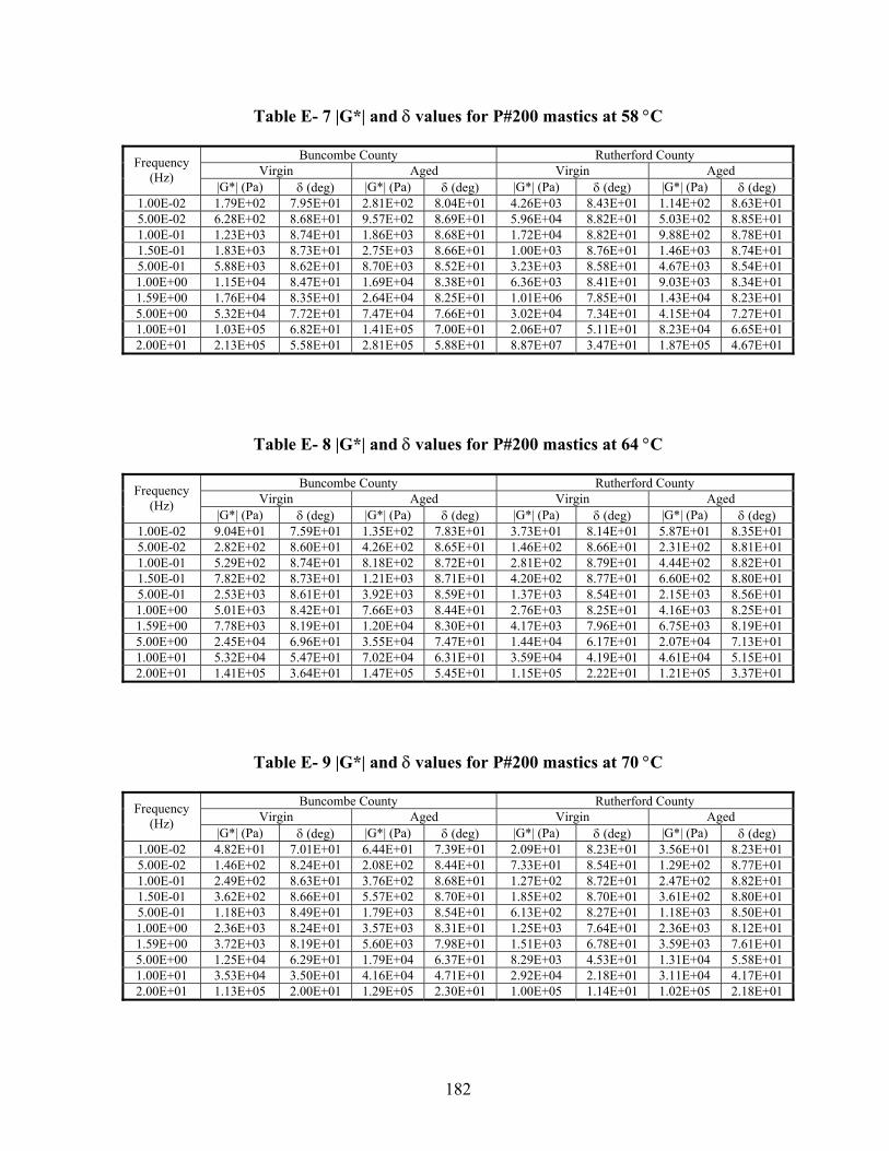
182
Table E- 7 |G*| and δ values for P#200 mastics at 58 °C
Buncombe County Rutherford County Virgin Aged Virgin Aged Frequency
(Hz) |G*| (Pa) δ (deg) |G*| (Pa) δ (deg) |G*| (Pa) δ (deg) |G*| (Pa) δ (deg)
1.00E-02 1.79E+02 7.95E+01 2.81E+02 8.04E+01 4.26E+03 8.43E+01 1.14E+02 8.63E+01 5.00E-02 6.28E+02 8.68E+01 9.57E+02 8.69E+01 5.96E+04 8.82E+01 5.03E+02 8.85E+01 1.00E-01 1.23E+03 8.74E+01 1.86E+03 8.68E+01 1.72E+04 8.82E+01 9.88E+02 8.78E+01 1.50E-01 1.83E+03 8.73E+01 2.75E+03 8.66E+01 1.00E+03 8.76E+01 1.46E+03 8.74E+01 5.00E-01 5.88E+03 8.62E+01 8.70E+03 8.52E+01 3.23E+03 8.58E+01 4.67E+03 8.54E+01 1.00E+00 1.15E+04 8.47E+01 1.69E+04 8.38E+01 6.36E+03 8.41E+01 9.03E+03 8.34E+01 1.59E+00 1.76E+04 8.35E+01 2.64E+04 8.25E+01 1.01E+06 7.85E+01 1.43E+04 8.23E+01 5.00E+00 5.32E+04 7.72E+01 7.47E+04 7.66E+01 3.02E+04 7.34E+01 4.15E+04 7.27E+01 1.00E+01 1.03E+05 6.82E+01 1.41E+05 7.00E+01 2.06E+07 5.11E+01 8.23E+04 6.65E+01 2.00E+01 2.13E+05 5.58E+01 2.81E+05 5.88E+01 8.87E+07 3.47E+01 1.87E+05 4.67E+01
Table E- 8 |G*| and δ values for P#200 mastics at 64 °C
Buncombe County Rutherford County Virgin Aged Virgin Aged Frequency
(Hz) |G*| (Pa) δ (deg) |G*| (Pa) δ (deg) |G*| (Pa) δ (deg) |G*| (Pa) δ (deg)
1.00E-02 9.04E+01 7.59E+01 1.35E+02 7.83E+01 3.73E+01 8.14E+01 5.87E+01 8.35E+01 5.00E-02 2.82E+02 8.60E+01 4.26E+02 8.65E+01 1.46E+02 8.66E+01 2.31E+02 8.81E+01 1.00E-01 5.29E+02 8.74E+01 8.18E+02 8.72E+01 2.81E+02 8.79E+01 4.44E+02 8.82E+01 1.50E-01 7.82E+02 8.73E+01 1.21E+03 8.71E+01 4.20E+02 8.77E+01 6.60E+02 8.80E+01 5.00E-01 2.53E+03 8.61E+01 3.92E+03 8.59E+01 1.37E+03 8.54E+01 2.15E+03 8.56E+01 1.00E+00 5.01E+03 8.42E+01 7.66E+03 8.44E+01 2.76E+03 8.25E+01 4.16E+03 8.25E+01 1.59E+00 7.78E+03 8.19E+01 1.20E+04 8.30E+01 4.17E+03 7.96E+01 6.75E+03 8.19E+01 5.00E+00 2.45E+04 6.96E+01 3.55E+04 7.47E+01 1.44E+04 6.17E+01 2.07E+04 7.13E+01 1.00E+01 5.32E+04 5.47E+01 7.02E+04 6.31E+01 3.59E+04 4.19E+01 4.61E+04 5.15E+01 2.00E+01 1.41E+05 3.64E+01 1.47E+05 5.45E+01 1.15E+05 2.22E+01 1.21E+05 3.37E+01
Table E- 9 |G*| and δ values for P#200 mastics at 70 °C
Buncombe County Rutherford County Virgin Aged Virgin Aged Frequency
(Hz) |G*| (Pa) δ (deg) |G*| (Pa) δ (deg) |G*| (Pa) δ (deg) |G*| (Pa) δ (deg)
1.00E-02 4.82E+01 7.01E+01 6.44E+01 7.39E+01 2.09E+01 8.23E+01 3.56E+01 8.23E+01 5.00E-02 1.46E+02 8.24E+01 2.08E+02 8.44E+01 7.33E+01 8.54E+01 1.29E+02 8.77E+01 1.00E-01 2.49E+02 8.63E+01 3.76E+02 8.68E+01 1.27E+02 8.72E+01 2.47E+02 8.82E+01 1.50E-01 3.62E+02 8.66E+01 5.57E+02 8.70E+01 1.85E+02 8.70E+01 3.61E+02 8.80E+01 5.00E-01 1.18E+03 8.49E+01 1.79E+03 8.54E+01 6.13E+02 8.27E+01 1.18E+03 8.50E+01 1.00E+00 2.36E+03 8.24E+01 3.57E+03 8.31E+01 1.25E+03 7.64E+01 2.36E+03 8.12E+01 1.59E+00 3.72E+03 8.19E+01 5.60E+03 7.98E+01 1.51E+03 6.78E+01 3.59E+03 7.61E+01 5.00E+00 1.25E+04 6.29E+01 1.79E+04 6.37E+01 8.29E+03 4.53E+01 1.31E+04 5.58E+01 1.00E+01 3.53E+04 3.50E+01 4.16E+04 4.71E+01 2.92E+04 2.18E+01 3.11E+04 4.17E+01 2.00E+01 1.13E+05 2.00E+01 1.29E+05 2.30E+01 1.00E+05 1.14E+01 1.02E+05 2.18E+01

183
Table E- 10 |G*|sin δ values for Buncombe County materials, 58 °C
Binder Baghouse Mastic P#200 Mastic Frequency (Hz) Virgin Aged Virgin Aged Virgin Aged
1.00E-02 2.13E+01 5.55E+01 2.54E+02 3.71E+02 1.76E+02 2.77E+02 5.00E-02 1.06E+02 2.74E+02 1.05E+03 1.56E+03 6.27E+02 9.56E+02 1.00E-01 2.12E+02 5.41E+02 1.98E+03 2.92E+03 1.22E+03 1.86E+03 1.50E-01 3.16E+02 8.01E+02 2.86E+03 4.28E+03 1.83E+03 2.74E+03 5.00E-01 1.03E+03 2.51E+03 8.86E+03 1.33E+04 5.86E+03 8.67E+03 1.00E+00 2.00E+03 4.76E+03 1.69E+04 2.51E+04 1.14E+04 1.68E+04 1.59E+00 3.10E+03 7.38E+03 2.75E+04 4.05E+04 1.75E+04 2.62E+04 5.00E+00 9.17E+03 2.00E+04 7.47E+04 1.08E+05 5.19E+04 7.26E+04 1.00E+01 1.74E+04 3.62E+04 1.37E+05 1.97E+05 9.60E+04 1.33E+05 2.00E+01 3.25E+04 6.47E+04 ** 3.63E+05 1.76E+05 2.40E+05 Average 6.58E+03 1.37E+04 3.01E+04 7.56E+04 3.63E+04 5.03E+04
Table E- 11 |G*|sin δ values for Buncombe County materials, 64 °C
Binder Baghouse Mastic P#200 Mastic Frequency (Hz) Virgin Aged Virgin Aged Virgin Aged
1.00E-02 9.10E+00 2.28E+01 1.16E+02 1.34E+02 8.77E+01 1.33E+02 5.00E-02 4.49E+01 1.14E+02 4.34E+02 5.94E+02 2.81E+02 4.25E+02 1.00E-01 9.00E+01 2.26E+02 8.12E+02 1.18E+03 5.29E+02 8.17E+02 1.50E-01 1.35E+02 3.37E+02 1.20E+03 1.75E+03 7.82E+02 1.21E+03 5.00E-01 4.46E+02 1.08E+03 3.66E+03 5.53E+03 2.53E+03 3.91E+03 1.00E+00 8.80E+02 2.09E+03 6.67E+03 1.05E+04 4.98E+03 7.63E+03 1.59E+00 1.35E+03 3.27E+03 1.05E+04 1.68E+04 7.71E+03 1.19E+04 5.00E+00 4.16E+03 9.20E+03 3.04E+04 4.75E+04 2.30E+04 3.42E+04 1.00E+01 7.97E+03 1.71E+04 5.62E+04 8.83E+04 4.34E+04 6.26E+04 2.00E+01 1.51E+04 3.08E+04 1.04E+05 1.61E+05 8.39E+04 1.20E+05 Average 3.02E+03 6.42E+03 2.14E+04 3.33E+04 1.67E+04 2.43E+04
Table E- 12 |G*|sin δ values for Buncombe County materials, 70 °C
Binder Baghouse Mastic P#200 Mastic Frequency (Hz) Virgin Aged Virgin Aged Virgin Aged
1.00E-02 4.24E+00 9.56E+00 5.33E+01 9.68E+01 4.53E+01 6.19E+01 5.00E-02 2.05E+01 4.72E+01 1.72E+02 3.53E+02 1.45E+02 2.07E+02 1.00E-01 4.10E+01 9.46E+01 3.11E+02 6.43E+02 2.49E+02 3.76E+02 1.50E-01 6.17E+01 1.41E+02 4.63E+02 9.92E+02 3.61E+02 5.56E+02 5.00E-01 2.05E+02 4.64E+02 1.47E+03 2.74E+03 1.18E+03 1.78E+03 1.00E+00 4.09E+02 9.11E+02 2.77E+03 4.74E+03 2.34E+03 3.54E+03 1.59E+00 6.33E+02 1.43E+03 5.18E+03 8.12E+03 3.69E+03 5.51E+03 5.00E+00 1.98E+03 4.17E+03 1.25E+04 2.13E+04 1.12E+04 1.61E+04 1.00E+01 3.84E+03 7.85E+03 2.40E+04 4.06E+04 2.03E+04 3.05E+04 2.00E+01 7.40E+03 1.45E+04 4.29E+04 7.55E+04 3.87E+04 5.06E+04 Average 1.46E+03 2.96E+03 8.97E+03 1.55E+04 7.81E+03 1.09E+04

184
Table E- 13 |G*|/sin δ values for Buncombe County materials, 58 °C
Binder Baghouse Mastic P#200 Mastic Frequency (Hz) Virgin Aged Virgin Aged Virgin Aged
1.00E-02 2.13E+01 5.55E+01 2.63E+02 3.77E+02 1.82E+02 2.85E+02 5.00E-02 1.06E+02 2.74E+02 1.06E+03 1.57E+03 6.29E+02 9.59E+02 1.00E-01 2.12E+02 5.42E+02 1.99E+03 2.93E+03 1.23E+03 1.86E+03 1.50E-01 3.16E+02 8.04E+02 2.88E+03 4.30E+03 1.83E+03 2.75E+03 5.00E-01 1.03E+03 2.53E+03 8.90E+03 1.33E+04 5.89E+03 8.73E+03 1.00E+00 2.01E+03 4.84E+03 1.70E+04 2.53E+04 1.15E+04 1.70E+04 1.59E+00 3.12E+03 7.54E+03 2.76E+04 4.08E+04 1.78E+04 2.67E+04 5.00E+00 9.28E+03 2.08E+04 7.47E+04 1.08E+05 5.46E+04 7.68E+04 1.00E+01 1.77E+04 3.82E+04 1.39E+05 1.97E+05 1.11E+05 1.50E+05 2.00E+01 3.34E+04 6.94E+04 ** 3.79E+05 2.58E+05 3.28E+05 Average 6.72E+03 1.45E+04 3.04E+04 7.73E+04 4.63E+04 6.14E+04
Table E- 14 |G*|/sin δ values for Buncombe County materials, 64 °C
Binder Baghouse Mastic P#200 Mastic Frequency (Hz) Virgin Aged Virgin Aged Virgin Aged
1.00E-02 9.11E+00 2.28E+01 1.23E+02 1.36E+02 9.32E+01 1.38E+02 5.00E-02 4.49E+01 1.14E+02 4.47E+02 5.97E+02 2.83E+02 4.27E+02 1.00E-01 9.00E+01 2.26E+02 8.27E+02 1.18E+03 5.30E+02 8.19E+02 1.50E-01 1.35E+02 3.37E+02 1.22E+03 1.75E+03 7.83E+02 1.21E+03 5.00E-01 4.46E+02 1.08E+03 3.67E+03 5.54E+03 2.54E+03 3.93E+03 1.00E+00 8.82E+02 2.09E+03 6.67E+03 1.05E+04 5.03E+03 7.70E+03 1.59E+00 1.35E+03 3.27E+03 1.06E+04 1.68E+04 7.86E+03 1.21E+04 5.00E+00 4.19E+03 9.20E+03 3.28E+04 4.81E+04 2.62E+04 3.68E+04 1.00E+01 8.06E+03 1.71E+04 7.87E+04 9.74E+04 6.51E+04 7.87E+04 2.00E+01 1.54E+04 3.08E+04 3.07E+05 2.50E+05 2.38E+05 1.81E+05 Average 3.06E+03 6.42E+03 4.42E+04 4.32E+04 3.46E+04 3.23E+04
Table E- 15 |G*|/sin δ values for Buncombe County materials, 70 °C
Binder Baghouse Mastic P#200 Mastic Frequency (Hz) Virgin Aged Virgin Aged Virgin Aged
1.00E-02 4.24E+00 9.56E+00 5.84E+01 1.07E+02 5.13E+01 6.71E+01 5.00E-02 2.05E+01 4.72E+01 1.78E+02 3.71E+02 1.48E+02 2.09E+02 1.00E-01 4.10E+01 9.46E+01 3.19E+02 6.67E+02 2.50E+02 3.77E+02 1.50E-01 6.17E+01 1.42E+02 4.70E+02 1.01E+03 3.62E+02 5.57E+02 5.00E-01 2.05E+02 4.65E+02 1.47E+03 2.76E+03 1.19E+03 1.79E+03 1.00E+00 4.09E+02 9.14E+02 2.79E+03 4.74E+03 2.38E+03 3.59E+03 1.59E+00 6.34E+02 1.44E+03 5.28E+03 8.14E+03 3.76E+03 5.69E+03 5.00E+00 1.99E+03 4.23E+03 1.98E+04 2.47E+04 1.41E+04 2.00E+04 1.00E+01 3.88E+03 8.03E+03 9.27E+04 7.10E+04 6.16E+04 5.68E+04 2.00E+01 7.57E+03 1.51E+04 4.50E+05 4.11E+05 3.31E+05 3.31E+05 Average 1.48E+03 3.05E+03 5.73E+04 5.25E+04 4.14E+04 4.20E+04

185
Table E- 16 |G*|cos δ values for Buncombe County materials, 58 °C
Binder Baghouse Mastic P#200 Mastic Frequency (Hz) Virgin Aged Virgin Aged Virgin Aged
1.00E-02 2.26E-01 6.48E-01 4.72E+01 4.81E+01 3.24E+01 4.66E+01 5.00E-02 1.31E+00 8.63E+00 1.15E+02 1.17E+02 3.47E+01 5.23E+01 1.00E-01 3.56E+00 2.63E+01 1.69E+02 1.85E+02 5.64E+01 1.02E+02 1.50E-01 6.31E+00 4.84E+01 2.18E+02 2.71E+02 8.54E+01 1.61E+02 5.00E-01 4.36E+01 2.54E+02 5.57E+02 9.76E+02 3.90E+02 7.23E+02 1.00E+00 1.21E+02 6.05E+02 1.01E+03 2.08E+03 1.06E+03 1.81E+03 1.59E+00 2.27E+02 1.09E+03 1.65E+03 3.75E+03 2.00E+03 3.46E+03 5.00E+00 9.92E+02 3.99E+03 8.53E+02 6.62E+03 1.18E+04 1.73E+04 1.00E+01 2.35E+03 8.43E+03 1.74E+04 5.50E+03 3.83E+04 4.83E+04 2.00E+01 5.56E+03 1.75E+04 ** 7.60E+04 1.20E+05 1.46E+05 Average 9.31E+02 3.19E+03 2.44E+03 9.55E+03 1.74E+04 2.17E+04
Table E- 17 |G*|cos δ values for Buncombe County materials, 64 °C
Binder Baghouse Mastic P#200 Mastic Frequency (Hz) Virgin Aged Virgin Aged Virgin Aged
1.00E-02 3.48E-01 1.33E-01 2.71E+01 1.64E+01 2.21E+01 2.74E+01 5.00E-02 5.27E-01 1.57E+00 7.40E+01 3.93E+01 1.97E+01 2.57E+01 1.00E-01 9.81E-01 5.37E+00 1.12E+02 6.83E+01 2.38E+01 3.93E+01 1.50E-01 1.80E+00 1.05E+01 1.31E+02 8.45E+01 3.67E+01 6.15E+01 5.00E-01 1.18E+01 7.16E+01 2.06E+02 2.06E+02 1.71E+02 2.79E+02 1.00E+00 3.31E+01 1.82E+02 9.28E+01 2.89E+02 5.07E+02 7.48E+02 1.59E+00 6.72E+01 3.45E+02 4.90E+02 2.74E+02 1.10E+03 1.46E+03 5.00E+00 3.46E+02 1.40E+03 8.54E+03 5.50E+03 8.56E+03 9.35E+03 1.00E+01 8.76E+02 3.14E+03 3.56E+04 2.84E+04 3.07E+04 3.18E+04 2.00E+01 2.25E+03 6.89E+03 1.45E+05 1.20E+05 1.14E+05 8.56E+04 Average 3.59E+02 1.20E+03 1.90E+04 1.54E+04 1.55E+04 1.29E+04
Table E- 18 |G*|cos δ values for Buncombe County materials, 70 °C
Binder Baghouse Mastic P#200 Mastic Frequency (Hz) Virgin Aged Virgin Aged Virgin Aged
1.00E-02 1.08E-01 1.18E-01 1.66E+01 3.12E+01 1.64E+01 1.79E+01 5.00E-02 3.40E-01 4.02E-01 3.30E+01 7.81E+01 1.94E+01 2.02E+01 1.00E-01 5.40E-01 1.19E+00 4.88E+01 1.22E+02 1.63E+01 2.08E+01 1.50E-01 7.81E-01 2.45E+00 5.85E+01 1.51E+02 2.12E+01 2.93E+01 5.00E-01 3.46E+00 1.83E+01 4.62E+01 2.32E+02 1.04E+02 1.43E+02 1.00E+00 9.91E+00 5.31E+01 2.06E+02 1.41E+02 3.11E+02 4.31E+02 1.59E+00 2.22E+01 1.06E+02 7.02E+02 3.98E+02 5.23E+02 9.95E+02 5.00E+00 1.35E+02 4.93E+02 9.56E+03 8.45E+03 5.71E+03 7.94E+03 1.00E+01 3.85E+02 1.19E+03 4.06E+04 3.51E+04 2.89E+04 2.83E+04 2.00E+01 1.12E+03 2.90E+03 1.32E+05 1.59E+05 1.06E+05 1.19E+05 Average 1.68E+02 4.77E+02 1.83E+04 2.04E+04 1.42E+04 1.57E+04

186
Table E- 19 |G*|sin δ values for Rutherford County materials, 58 °C
Binder Baghouse Mastic P#200 Mastic Frequency (Hz) Virgin Aged Virgin Aged Virgin Aged
1.00E-02 1.58E+01 4.79E+01 1.61E+02 1.61E+02 *** 1.14E+02 5.00E-02 7.84E+01 2.35E+02 6.13E+02 5.94E+02 *** 5.03E+02 1.00E-01 1.57E+02 4.62E+02 1.20E+03 1.17E+03 *** 9.87E+02 1.50E-01 2.34E+02 6.85E+02 1.79E+03 1.75E+03 *** 1.46E+03 5.00E-01 7.67E+02 2.14E+03 5.76E+03 5.50E+03 *** 4.65E+03 1.00E+00 1.50E+03 4.07E+03 1.12E+04 1.07E+04 *** 8.97E+03 1.59E+00 2.36E+03 6.28E+03 1.70E+04 1.66E+04 *** 1.41E+04 5.00E+00 6.92E+03 1.70E+04 4.96E+04 4.72E+04 *** 3.96E+04 1.00E+01 1.32E+04 3.09E+04 9.18E+04 8.69E+04 *** 7.54E+04 2.00E+01 2.45E+04 5.44E+04 1.67E+05 1.61E+05 *** 1.36E+05 Average 4.97E+03 1.16E+04 3.46E+04 3.31E+04 *** 2.82E+04
Table E- 20 |G*|sin δ values for Rutherford County materials, 64 °C
Binder Baghouse Mastic P#200 Mastic Frequency (Hz) Virgin Aged Virgin Aged Virgin Aged
1.00E-02 6.96E+00 1.94E+01 8.49E+01 7.91E+01 3.69E+01 5.83E+01 5.00E-02 3.38E+01 9.63E+01 2.71E+02 2.63E+02 1.46E+02 2.31E+02 1.00E-01 6.78E+01 1.93E+02 5.15E+02 4.99E+02 2.81E+02 4.44E+02 1.50E-01 1.02E+02 2.88E+02 7.65E+02 7.43E+02 4.20E+02 6.60E+02 5.00E-01 3.35E+02 9.25E+02 2.47E+03 2.41E+03 1.36E+03 2.15E+03 1.00E+00 6.63E+02 1.78E+03 4.83E+03 4.71E+03 2.73E+03 4.12E+03 1.59E+00 1.05E+03 2.76E+03 7.51E+03 7.36E+03 4.10E+03 6.68E+03 5.00E+00 3.14E+03 7.83E+03 2.27E+04 2.18E+04 1.27E+04 1.96E+04 1.00E+01 6.04E+03 1.45E+04 4.22E+04 4.04E+04 2.40E+04 3.61E+04 2.00E+01 1.15E+04 2.64E+04 8.08E+04 7.59E+04 4.34E+04 6.70E+04 Average 2.29E+03 5.48E+03 1.62E+04 1.54E+04 8.91E+03 1.37E+04
Table E- 21 |G*|sin δ values for Rutherford County materials, 70 °C
Binder Baghouse Mastic P#200 Mastic Frequency (Hz) Virgin Aged Virgin Aged Virgin Aged
1.00E-02 3.29E+00 8.24E+00 4.14E+01 4.21E+01 2.07E+01 3.52E+01 5.00E-02 1.65E+01 4.02E+01 1.35E+02 1.29E+02 7.30E+01 1.29E+02 1.00E-01 3.29E+01 8.11E+01 2.30E+02 2.24E+02 1.27E+02 2.47E+02 1.50E-01 4.95E+01 1.21E+02 3.37E+02 3.27E+02 1.85E+02 3.60E+02 5.00E-01 1.64E+02 3.98E+02 1.10E+03 1.07E+03 6.08E+02 1.17E+03 1.00E+00 3.27E+02 7.81E+02 2.17E+03 2.09E+03 1.21E+03 2.33E+03 1.59E+00 5.15E+02 1.22E+03 3.22E+03 3.14E+03 1.39E+03 3.48E+03 5.00E+00 1.58E+03 3.56E+03 1.01E+04 1.01E+04 5.89E+03 1.09E+04 1.00E+01 3.07E+03 6.72E+03 1.89E+04 2.00E+04 1.09E+04 2.07E+04 2.00E+01 5.87E+03 1.24E+04 3.57E+04 3.50E+04 1.98E+04 3.78E+04 Average 1.16E+03 2.54E+03 7.19E+03 7.23E+03 4.02E+03 7.71E+03

187
Table E- 22 |G*|/sin δ values for Rutherford County materials, 58 °C
Binder Baghouse Mastic P#200 Mastic Frequency (Hz) Virgin Aged Virgin Aged Virgin Aged
1.00E-02 1.58E+01 4.79E+01 1.65E+02 1.64E+02 *** 1.14E+02 5.00E-02 7.84E+01 2.35E+02 6.14E+02 5.95E+02 *** 5.03E+02 1.00E-01 1.57E+02 4.64E+02 1.21E+03 1.17E+03 *** 9.88E+02 1.50E-01 2.34E+02 6.88E+02 1.80E+03 1.75E+03 *** 1.47E+03 5.00E-01 7.68E+02 2.17E+03 5.79E+03 5.53E+03 *** 4.68E+03 1.00E+00 1.51E+03 4.13E+03 1.13E+04 1.08E+04 *** 9.09E+03 1.59E+00 2.37E+03 6.42E+03 1.73E+04 1.69E+04 *** 1.44E+04 5.00E+00 6.99E+03 1.77E+04 5.27E+04 5.07E+04 *** 4.35E+04 1.00E+01 1.34E+04 3.25E+04 1.09E+05 1.06E+05 *** 8.97E+04 2.00E+01 2.52E+04 5.83E+04 2.60E+05 2.56E+05 *** 2.57E+05 Average 5.07E+03 1.23E+04 4.60E+04 4.50E+04 *** 4.21E+04
Table E- 23 |G*|/sin δ values for Rutherford County materials, 64 °C
Binder Baghouse Mastic P#200 Mastic Frequency (Hz) Virgin Aged Virgin Aged Virgin Aged
1.00E-02 6.96E+00 1.94E+01 8.87E+01 8.26E+01 3.77E+01 5.91E+01 5.00E-02 3.39E+01 9.63E+01 2.72E+02 2.64E+02 1.47E+02 2.32E+02 1.00E-01 6.78E+01 1.93E+02 5.16E+02 4.99E+02 2.81E+02 4.44E+02 1.50E-01 1.02E+02 2.88E+02 7.66E+02 7.44E+02 4.21E+02 6.60E+02 5.00E-01 3.35E+02 9.29E+02 2.48E+03 2.42E+03 1.37E+03 2.16E+03 1.00E+00 6.64E+02 1.80E+03 4.89E+03 4.77E+03 2.78E+03 4.19E+03 1.59E+00 1.05E+03 2.79E+03 7.67E+03 7.53E+03 4.24E+03 6.81E+03 5.00E+00 3.16E+03 8.02E+03 2.54E+04 2.44E+04 1.63E+04 2.19E+04 1.00E+01 6.11E+03 1.50E+04 6.40E+04 6.04E+04 5.38E+04 5.90E+04 2.00E+01 1.18E+04 2.77E+04 2.05E+05 2.12E+05 3.03E+05 2.18E+05 Average 2.33E+03 5.68E+03 3.11E+04 3.13E+04 3.83E+04 3.14E+04
Table E- 24 |G*|/sin δ values for Rutherford County materials, 70 °C
Binder Baghouse Mastic P#200 Mastic Frequency (Hz) Virgin Aged Virgin Aged Virgin Aged
1.00E-02 3.29E+00 8.25E+00 4.53E+01 4.64E+01 2.11E+01 3.59E+01 5.00E-02 1.65E+01 4.02E+01 1.37E+02 1.30E+02 7.35E+01 1.29E+02 1.00E-01 3.29E+01 8.12E+01 2.31E+02 2.25E+02 1.27E+02 2.47E+02 1.50E-01 4.95E+01 1.21E+02 3.38E+02 3.28E+02 1.86E+02 3.61E+02 5.00E-01 1.64E+02 3.99E+02 1.11E+03 1.08E+03 6.18E+02 1.18E+03 1.00E+00 3.28E+02 7.84E+02 2.23E+03 2.15E+03 1.28E+03 2.38E+03 1.59E+00 5.15E+02 1.22E+03 3.41E+03 3.30E+03 1.63E+03 3.70E+03 5.00E+00 1.59E+03 3.62E+03 1.56E+04 1.34E+04 1.16E+04 1.59E+04 1.00E+01 3.10E+03 6.88E+03 6.07E+04 4.43E+04 7.85E+04 4.68E+04 2.00E+01 6.02E+03 1.30E+04 3.59E+05 3.22E+05 5.09E+05 2.73E+05 Average 1.18E+03 2.61E+03 4.42E+04 3.87E+04 6.03E+04 3.44E+04

188
Table E- 25 |G*|cos δ values for Rutherford County materials, 58 °C
Binder Baghouse Mastic P#200 Mastic Frequency (Hz) Virgin Aged Virgin Aged Virgin Aged
1.00E-02 2.62E-01 6.17E-01 2.47E+01 2.26E+01 *** 7.31E+00 5.00E-02 6.74E-01 7.60E+00 2.50E+01 2.30E+01 *** 1.33E+01 1.00E-01 2.43E+00 2.33E+01 4.73E+01 4.55E+01 *** 3.78E+01 1.50E-01 4.62E+00 4.23E+01 7.72E+01 7.22E+01 *** 6.73E+01 5.00E-01 3.04E+01 2.20E+02 3.97E+02 4.21E+02 *** 3.75E+02 1.00E+00 8.49E+01 5.27E+02 1.10E+03 1.15E+03 *** 1.04E+03 1.59E+00 1.61E+02 9.31E+02 2.10E+03 2.16E+03 *** 1.92E+03 5.00E+00 7.18E+02 3.36E+03 1.25E+04 1.29E+04 *** 1.23E+04 1.00E+01 1.70E+03 7.07E+03 3.93E+04 4.10E+04 *** 3.29E+04 2.00E+01 4.06E+03 1.45E+04 1.25E+05 1.24E+05 *** 1.28E+05 Average 6.76E+02 2.67E+03 1.80E+04 1.82E+04 *** 1.77E+04
Table E- 26 |G*|cos δ values for Rutherford County materials, 64 °C
Binder Baghouse Mastic P#200 Mastic Frequency (Hz) Virgin Aged Virgin Aged Virgin Aged
1.00E-02 9.46E-02 1.92E-01 1.81E+01 1.67E+01 5.59E+00 6.64E+00 5.00E-02 3.31E-01 1.53E+00 1.66E+01 1.42E+01 8.65E+00 7.70E+00 1.00E-01 5.89E-01 5.08E+00 2.00E+01 1.88E+01 1.02E+01 1.40E+01 1.50E-01 1.29E+00 1.02E+01 3.13E+01 3.08E+01 1.69E+01 2.32E+01 5.00E-01 8.32E+00 6.24E+01 1.69E+02 1.73E+02 1.10E+02 1.65E+02 1.00E+00 2.32E+01 1.60E+02 5.48E+02 5.24E+02 3.59E+02 5.46E+02 1.59E+00 4.96E+01 2.99E+02 1.10E+03 1.12E+03 7.56E+02 9.47E+02 5.00E+00 2.60E+02 1.20E+03 7.84E+03 7.58E+03 6.81E+03 6.65E+03 1.00E+01 6.78E+02 2.66E+03 3.03E+04 2.85E+04 2.67E+04 2.87E+04 2.00E+01 1.85E+03 5.78E+03 1.00E+05 1.02E+05 1.06E+05 1.01E+05 Average 2.87E+02 1.02E+03 1.40E+04 1.40E+04 1.41E+04 1.38E+04
Table E- 27 |G*|cos δ values for Rutherford County materials, 70 °C
Binder Baghouse Mastic P#200 Mastic Frequency (Hz) Virgin Aged Virgin Aged Virgin Aged
1.00E-02 6.13E-02 8.51E-02 1.26E+01 1.34E+01 2.78E+00 4.73E+00 5.00E-02 2.08E-01 3.10E-01 1.70E+01 1.29E+01 5.89E+00 5.07E+00 1.00E-01 2.73E-01 1.01E+00 1.39E+01 1.24E+01 6.17E+00 7.62E+00 1.50E-01 5.18E-01 2.12E+00 1.73E+01 1.73E+01 9.72E+00 1.23E+01 5.00E-01 2.46E+00 1.60E+01 9.88E+01 1.03E+02 7.80E+01 1.03E+02 1.00E+00 7.19E+00 4.69E+01 3.52E+02 3.40E+02 2.94E+02 3.59E+02 1.59E+00 1.65E+01 9.14E+01 7.69E+02 7.07E+02 5.69E+02 8.63E+02 5.00E+00 1.04E+02 4.32E+02 7.42E+03 5.74E+03 5.82E+03 7.39E+03 1.00E+01 2.93E+02 1.05E+03 2.81E+04 2.20E+04 2.71E+04 2.32E+04 2.00E+01 9.25E+02 2.58E+03 1.07E+05 1.00E+05 9.83E+04 9.43E+04 Average 1.35E+02 4.22E+02 1.44E+04 1.29E+04 1.32E+04 1.26E+04

189
Appendix F
Mobilized Interfacial Shear Stresses

190
-2
-1
0
1
2
3
4
0 10 20 30 40 50 60
Shear Stress, psi
Dis
tanc
e R
atio
, d/a
0.5in1.5in2.5in3.5in4.5in
(a) Shear distribution along axle for vertical load with
zero horizontal shear
0
10
20
30
40
50
60
70
80
-4 -3 -2 -1 0 1 2 3 4Distance Ratio, d/a
She
ar S
tress
, psi
0.5in1.5in2.5in3.5in4.5in
(b) Shear distribution perpendicular to axle for
vertical load with zero horizontal shear
-2
-1
0
1
2
3
4
0 10 20 30 40 50 60
Shear Stress, psi
Dis
tanc
e R
atio
, d/a
0.5in1.5in2.5in3.5in4.5in
(c) Shear distribution along axle for vertical load with
40% horizontal shear
0
10
20
30
40
50
60
70
80
-4 -3 -2 -1 0 1 2 3 4Distance Ratio, d/a
She
ar S
tress
, psi
0.5in1.5in2.5in3.5in4.5in
(d) Shear distribution perpendicular to axle for
vertical load with 40% horizontal shear
-2
-1
0
1
2
3
4
0 10 20 30 40 50 60
Shear Stress, psi
Dis
tanc
e R
atio
, d/a
0.5in1.5in2.5in3.5in4.5in
(e) Shear distribution along axle for vertical load with
70% horizontal shear
0
10
20
30
40
50
60
70
80
-4 -3 -2 -1 0 1 2 3 4Distance Ratio, d/a
She
ar S
tress
, psi
0.5in1.5in2.5in3.5in4.5in
(f) Shear distribution perpendicular to axle for vertical
load with 70% horizontal shear
Figure F-1(a-f) Mobilized interfacial shear stresses for AC-AC combination at 20 °C

191
-2
-1
0
1
2
3
4
0 10 20 30 40 50 60
Shear Stress, psi
Dis
tanc
e R
atio
, d/a
0.5in1.5in2.5in3.5in4.5in5.5in
(a) Shear distribution along axle for vertical load with
zero horizontal shear
0
10
20
30
40
50
60
70
80
-4 -3 -2 -1 0 1 2 3 4Distance Ratio, d/a
She
ar S
tress
, psi
0.5in1.5in2.5in3.5in4.5in5.5in
(b) Shear distribution perpendicular to axle for
vertical load with zero horizontal shear
-2
-1
0
1
2
3
4
0 10 20 30 40 50 60
Shear Stress, psi
Dis
tanc
e R
atio
, d/a
0.5in1.5in2.5in3.5in4.5in5.5in
(c) Shear distribution along axle for vertical load with
40% horizontal shear
0
10
20
30
40
50
60
70
80
-4 -3 -2 -1 0 1 2 3 4Distance Ratio, d/a
She
ar S
tress
, psi
0.5in1.5in2.5in3.5in4.5in5.5in
(d) Shear distribution perpendicular to axle for
vertical load with 40% horizontal shear
-2
-1
0
1
2
3
4
0 10 20 30 40 50 60
Shear Stress, psi
Dis
tanc
e R
atio
, d/a
0.5in1.5in2.5in3.5in4.5in5.5in
(e) Shear distribution along axle for vertical load with
70% horizontal shear
0
10
20
30
40
50
60
70
80
-4 -3 -2 -1 0 1 2 3 4Distance Ratio, d/a
She
ar S
tress
, psi
0.5in1.5in2.5in3.5in4.5in5.5in
(f) Shear distribution perpendicular to axle for vertical load with 70% horizontal shear
Figure F-2(a-f) Mobilized interfacial shear stresses for AC-AC, high temp.

192
-2
-1
0
1
2
3
4
0 10 20 30 40 50 60
Shear Stress, psi
Dis
tanc
e R
atio
, d/a
0.5in1.5in2.5in3.5in4.5in
(a) Shear distribution along axle for vertical load with
zero horizontal shear
0
10
20
30
40
50
60
70
80
-4 -3 -2 -1 0 1 2 3 4Distance Ratio, d/a
She
ar S
tress
, psi
0.5in1.5in2.5in3.5in4.5in
(b) Shear distribution perpendicular to axle for
vertical load with zero horizontal shear
-2
-1
0
1
2
3
4
0 10 20 30 40 50 60
Shear Stress, psi
Dis
tanc
e R
atio
, d/a
0.5in1.5in2.5in3.5in4.5in
(c) Shear distribution along axle for vertical load with
40% horizontal shear
0
10
20
30
40
50
60
70
80
-4 -3 -2 -1 0 1 2 3 4Distance Ratio, d/a
She
ar S
tress
, psi
0.5in1.5in2.5in3.5in4.5in
(d) Shear distribution perpendicular to axle for
vertical load with 40% horizontal shear
-2
-1
0
1
2
3
4
0 10 20 30 40 50 60 70
Shear Stress, psi
Dis
tanc
e R
atio
, d/a
0.5in1.5in2.5in3.5in4.5in
(e) Shear distribution along axle for vertical load with
70% horizontal shear
0
10
20
30
40
50
60
70
80
-4 -3 -2 -1 0 1 2 3 4Distance Ratio, d/a
She
ar S
tress
, psi
0.5in1.5in2.5in3.5in4.5in
(f) Shear distribution perpendicular to axle for vertical load with 70% horizontal shear
Figure F-3(a-f) Mobilized interfacial shear stresses for PCC-AC, 20 °C

193
-2
-1
0
1
2
3
4
0 10 20 30 40 50 60
Shear Stress, psi
Dis
tanc
e R
atio
, d/a
0.5in1.5in2.5in3.5in4.5in5.5in
(a) Shear distribution along axle for vertical load with
zero horizontal shear
0
10
20
30
40
50
60
70
80
-4 -3 -2 -1 0 1 2 3 4Distance Ratio, d/a
She
ar S
tress
, psi
0.5in1.5in2.5in3.5in4.5in5.5in
(b) Shear distribution perpendicular to axle for
vertical load with zero horizontal shear
-2
-1
0
1
2
3
4
0 10 20 30 40 50 60
Shear Stress, psi
Dis
tanc
e R
atio
, d/a
0.5in1.5in2.5in3.5in4.5in5.5in
(c) Shear distribution along axle for vertical load with
40% horizontal shear
0
10
20
30
40
50
60
70
80
-4 -3 -2 -1 0 1 2 3 4Distance Ratio, d/a
She
ar S
tress
, psi
0.5in1.5in2.5in3.5in4.5in5.5in
(d) Shear distribution perpendicular to axle for
vertical load with 40% horizontal shear
-2
-1
0
1
2
3
4
0 10 20 30 40 50 60 70
Shear Stress, psi
Dis
tanc
e R
atio
, d/a
0.5in1.5in2.5in3.5in4.5in5.5in
(e) Shear distribution along axle for vertical load with
70% horizontal shear
0
10
20
30
40
50
60
70
80
-4 -3 -2 -1 0 1 2 3 4Distance Ratio, d/a
She
ar S
tress
, psi
0.5in1.5in2.5in3.5in4.5in5.5in
(f) Shear distribution perpendicular to axle for vertical
load with 70% horizontal shear
Figure F-4 (a-f) Mobilized interfacial shear stresses for PCC-AC, high temp.

194
-2
-1
0
1
2
3
4
0 10 20 30 40 50 60
Shear Stress, psi
Dis
tanc
e R
atio
, d/a
0.5in1.5in2.5in3.5in4.5in5.5in6.5in
(a) Shear distribution along axle for vertical load with
zero horizontal shear
0
10
20
30
40
50
60
70
80
-4 -3 -2 -1 0 1 2 3 4Distance Ratio, d/a
She
ar S
tress
, psi
0.5in1.5in2.5in3.5in4.5in5.5in6.5in
(b) Shear distribution perpendicular to axle for
vertical load with zero horizontal shear
-2
-1
0
1
2
3
4
0 10 20 30 40 50 60
Shear Stress, psi
Dis
tanc
e R
atio
, d/a
0.5in1.5in2.5in3.5in4.5in5.5in6.5in
(c) Shear distribution along axle for vertical load with
40% horizontal shear
0
10
20
30
40
50
60
70
80
-4 -3 -2 -1 0 1 2 3 4Distance Ratio, d/a
She
ar S
tress
, psi
0.5in1.5in2.5in3.5in4.5in5.5in6.5in
(d) Shear distribution perpendicular to axle for
vertical load with 40% horizontal shear
-2
-1
0
1
2
3
4
0 10 20 30 40 50 60
Shear Stress, psi
Dis
tanc
e R
atio
, d/a
0.5in1.5in2.5in3.5in4.5in5.5in6.5in
(e) Shear distribution along axle for vertical load with
70% horizontal shear
0
10
20
30
40
50
60
70
80
-4 -3 -2 -1 0 1 2 3 4Distance Ratio, d/a
She
ar S
tress
, psi
0.5in1.5in2.5in3.5in4.5in5.5in6.5in
(f) Shear distribution perpendicular to axle for
vertical load with 70% horizontal shear
Figure F-5(a-f) Mobilized interfacial shear stresses for CTB-AC, 20 °C

195
-2
-1
0
1
2
3
4
0 10 20 30 40 50 60
Shear Stress, psi
Dis
tanc
e R
atio
, d/a
0.5in1.5in2.5in3.5in4.5in5.5in6.5in
(a) Shear distribution along axle for vertical load with
zero horizontal shear
0
10
20
30
40
50
60
70
80
-4 -3 -2 -1 0 1 2 3 4Distance Ratio, d/a
She
ar S
tress
, psi
0.5in1.5in2.5in3.5in4.5in5.5in6.5in
(b) Shear distribution perpendicular to axle for
vertical load with zero horizontal shear
-2
-1
0
1
2
3
4
0 10 20 30 40 50 60
Shear Stress, psi
Dis
tanc
e R
atio
, d/a
0.5in1.5in2.5in3.5in4.5in5.5in6.5in
(c) Shear distribution along axle for vertical load with
40% horizontal shear
0
10
20
30
40
50
60
70
80
-4 -3 -2 -1 0 1 2 3 4Distance Ratio, d/a
She
ar S
tress
, psi
0.5in1.5in2.5in3.5in4.5in5.5in6.5in
(d) Shear distribution perpendicular to axle for
vertical load with 40% horizontal shear
-2
-1
0
1
2
3
4
0 10 20 30 40 50 60 70
Shear Stress, psi
Dis
tanc
e R
atio
, d/a
0.5in1.5in2.5in3.5in4.5in5.5in6.5in
(e) Shear distribution along axle for vertical load with
70% horizontal shear
0
10
20
30
40
50
60
70
80
-4 -3 -2 -1 0 1 2 3 4Distance Ratio, d/a
She
ar S
tress
, psi
0.5in1.5in2.5in3.5in4.5in5.5in6.5in
(f) Shear distribution perpendicular to axle for vertical load with 70% horizontal shear
Figure F-6(a-f) Mobilized interfacial shear stresses for CTB-AC, high temp.