EFFECT OF SPIKES INTEGRATED TO AIRFOIL AT SUPERSONIC … · 2019-04-21 · Keywords: NACA 651-412...
13
IJRET: International Journal of Research in Engineering and Technology eISSN: 2319-1163 | pISSN: 2321-7308 _______________________________________________________________________________________ Volume: 03 Issue: 10 | Oct-2014, Available @ http://www.ijret.org 226 EFFECT OF SPIKES INTEGRATED TO AIRFOIL AT SUPERSONIC SPEED Md Akhtar Khan 1 , Karrothu Vigneshwara 2 , Suresh Kukutla 3 , Avinash Gupta 4 1 Assistant Professor, GITAM University-Hyderabad 2 Student, GNITC 3 Asst. Professor, GNITC 4 Student, GITAM University, Hyderabad Abstract The objective of this is to analyse the flow field over an aerofoil section integrated with spikes at supersonic speed (Mach number greater than 1). Use of spike integrated with aerofoil changes the flow characteristics over aerofoil and hence aerodynamic lift and drag. The experiment consists of flow visualization graphs and measurement of coefficient of aerodynamic drag and lift. Here we are using different shapes of spike like sharp edge and hemi spherical edge. In this we will compare the flow over aerofoil with spike and without spike. The flow analysis is done by using Computational fluid dynamics (CFD). CFD is the study of external flow over a body or internal flow through the body. CFD is aiding aero-dynamist to better understand the flow physics and in turn to design efficient models. In short, CFD is playing a strong role as a design tool as well as a research tool. Keywords: NACA 651-412 airfoil, spike, Ansys Fluent, Ansys ICEM CFD, Pressure Coefficient -------------------------------------------------------------------***---------------------------------------------------------------------- 1. INTRODUCTION While travelling at supersonic/ hypersonic speeds, the formation of detached shock wave leads to higher aerodynamic heating and drag. The boundary layer separation will immediately starts at mid of aerofoil. This leads to turbulence flow on it. Due to turbulence flow the temperature gradient and velocity gradient will be high. So the after effect may be either loss in performance or erosion/ablation of the surface of aerofoil. In order to alleviate these problems, various techniques are being studied, e.g., integration of spikes etc.[1] Fig 1.1 Heat Transfer [2] Fig 1.2 Heating of the body [2] Fig 1.3 Normal Fig 1.4 With Sharp Spike Fig 1.5 With Hemispherical Spike Use of spike seems to be a simple preposition and it has been studied in details in last few decades. The flow field around an aerofoil will get modified due to presence of a simple spike having sharp tip. [3] The flow field between the tip of spike and the aerofoil will strongly depend on incoming free stream flow conditions, shape of the tip of spike, length and diameter of stem which is connecting the spike tip to the aerofoil, etc. The presence of spike, leads to formation of a weaker spike shock, separated zone and separation shock due to adverse pressure gradient, recirculation zone, shear layer, etc. Due to the presence of recirculation in separated zone, major part of the aerofoil will experience lesser pressure and hence reduction in drag.
Transcript of EFFECT OF SPIKES INTEGRATED TO AIRFOIL AT SUPERSONIC … · 2019-04-21 · Keywords: NACA 651-412...
IJRET: International Journal of Research in Engineering and Technology eISSN: 2319-1163 | pISSN: 2321-7308
_______________________________________________________________________________________
Volume: 03 Issue: 10 | Oct-2014, Available @ http://www.ijret.org 226
EFFECT OF SPIKES INTEGRATED TO AIRFOIL AT SUPERSONIC
SPEED
Md Akhtar Khan1, Karrothu Vigneshwara
2, Suresh Kukutla
3, Avinash Gupta
4
1Assistant Professor, GITAM University-Hyderabad
2Student, GNITC
3Asst. Professor, GNITC
4Student, GITAM University, Hyderabad
Abstract The objective of this is to analyse the flow field over an aerofoil section integrated with spikes at supersonic speed (Mach number
greater than 1). Use of spike integrated with aerofoil changes the flow characteristics over aerofoil and hence aerodynamic lift
and drag. The experiment consists of flow visualization graphs and measurement of coefficient of aerodynamic drag and lift.
Here we are using different shapes of spike like sharp edge and hemi spherical edge. In this we will compare the flow over
aerofoil with spike and without spike. The flow analysis is done by using Computational fluid dynamics (CFD). CFD is the study
of external flow over a body or internal flow through the body. CFD is aiding aero-dynamist to better understand the flow physics
and in turn to design efficient models. In short, CFD is playing a strong role as a design tool as well as a research tool.
Keywords: NACA 651-412 airfoil, spike, Ansys Fluent, Ansys ICEM CFD, Pressure Coefficient
-------------------------------------------------------------------***----------------------------------------------------------------------
1. INTRODUCTION
While travelling at supersonic/ hypersonic speeds, the
formation of detached shock wave leads to higher
aerodynamic heating and drag. The boundary layer
separation will immediately starts at mid of aerofoil. This
leads to turbulence flow on it. Due to turbulence flow the
temperature gradient and velocity gradient will be high. So
the after effect may be either loss in performance or
erosion/ablation of the surface of aerofoil. In order to alleviate these problems, various techniques are being
studied, e.g., integration of spikes etc.[1]
Fig 1.1 Heat Transfer [2]
Fig 1.2 Heating of the body [2]
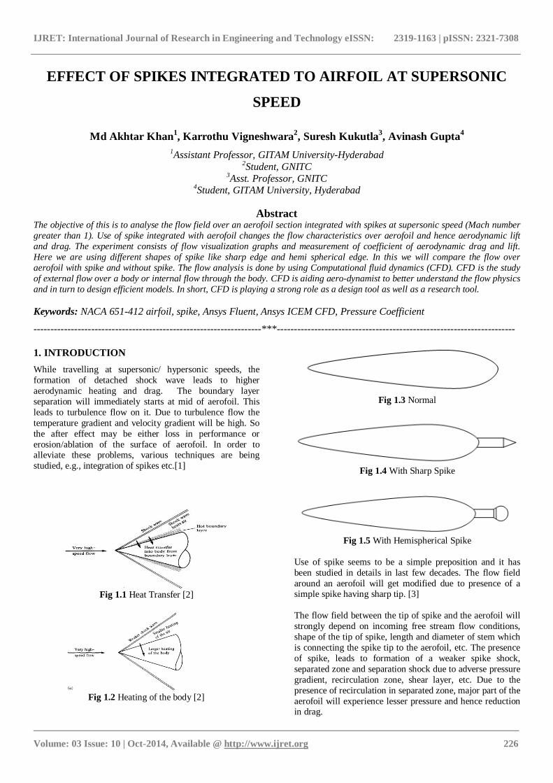
Fig 1.3 Normal
Fig 1.4 With Sharp Spike
Fig 1.5 With Hemispherical Spike
Use of spike seems to be a simple preposition and it has
been studied in details in last few decades. The flow field
around an aerofoil will get modified due to presence of a simple spike having sharp tip. [3]
The flow field between the tip of spike and the aerofoil will
strongly depend on incoming free stream flow conditions,
shape of the tip of spike, length and diameter of stem which
is connecting the spike tip to the aerofoil, etc. The presence
of spike, leads to formation of a weaker spike shock,
separated zone and separation shock due to adverse pressure
gradient, recirculation zone, shear layer, etc. Due to the
presence of recirculation in separated zone, major part of the
aerofoil will experience lesser pressure and hence reduction in drag.

IJRET: International Journal of Research in Engineering and Technology eISSN: 2319-1163 | pISSN: 2321-7308
_______________________________________________________________________________________
Volume: 03 Issue: 10 | Oct-2014, Available @ http://www.ijret.org 227
The present investigation aims to obtain the flow field
around an airfoil in the presence of either a sharp spike or
hemispherical head spike at supersonic speed. Experiments
and computations are made to obtain the overall flow field
and drag, in the presence of either a sharp or hemispherical
head spike.[4]
1.1 Geometry
For this study, the NACA 6-series airfoil is selected. A brief
description about the NACA 6-series is given as follows.
The NACA 6-Series was derived using an improved
theoretical method that, like the 1-Series, relied on
specifying the desired pressure distribution and employed
advanced mathematics to derive the required geometrical
shape. The goal of this approach was to design aerofoils that
maximized the region over which the airflow remains
laminar. In so doing, the drag over a small l range of lift
coefficients can be substantially reduced. The naming
convention of the 6-Series is by far the most confusing of any of the families discussed thus far, especially since many
different variations exist. [6]
In this example, 6 denote the series and indicate that this
family is designed for greater laminar flow than the Four- or
Five-Digit Series. The second digit, 5, is the location of the
minimum pressure in tenths of chord (0.5c). The subscript
‗1‘ indicates that low drag is maintained at lift coefficients
0.1 above and below the design lift coefficient (0.4)
specified by the first digit after the dash in tenths. The final
two digits specify the thickness in percentage of chord, 12%. The fraction specified indicates the percentage of the
aerofoil chord over which the pressure distribution on the
aerofoil is uniform. If not specified, the quantity is assumed
to be 1, or the distribution is constant over the entire
aerofoil.
The NACA 651-412airfoil of the NACA 6-series airfoils is
selected for the present study. Two different spike shapes
have been designed to integrate to the airfoil. One of the
spikes has a sharp tip, while the other spike had a
hemispherical tip. These spikes are attached to airfoil at the
leading edge. The spike geometries are shown in the figures fig 1.6 & fig 1.7
Fig 1.6 Sharp Edge
Fig 1.7 Hemi Spherical Edge
Computational Fluid Dynamics
Computational fluid dynamics, usually abbreviated as CFD,
is a branch of fluid mechanics that uses numerical methods and algorithms to solve and analyze problems that involve
fluid flows. Computers are used to perform the calculations
required to simulate the interaction of liquids and gases with
surfaces defined by boundary conditions. With high-speed
supercomputers, better solutions can be achieved. Ongoing
research yields software that improves the accuracy and
speed of complex simulation scenarios such as transonic or
turbulent flows. Initial experimental validation of such
software is performed using a wind tunnel with the final
validation coming in full-scale testing, e.g. flight tests.[5]
2. METHODOLOGY
In all of these approaches the same basic procedure is followed.
During pre-processing
(i) The geometry (physical bounds) of the problem is
defined.
(ii) The volume occupied by the fluid is divided into
discrete cells (the mesh). The mesh may be uniform or non
uniform.
(iii) The physical modelling is defined – for example, the
equations of motions + enthalpy + radiation + species
conservation
(iv)Boundary conditions are defined. This involves specifying the fluid behaviour and properties at the
boundaries of the problem. For transient problems, the
initial conditions are also defined.
(v) The simulation is started and the equations are solved
iteratively as a steady-state or transient.
(vi)Finally a postprocessor is used for the analysis and
visualization of the resulting solution.
2.1 Software Packages Used
2.1.1 ANSYS ICEM CFD:
ANSYS ICEM CFD meshing software starts with advanced
CAD/geometry readers and repair tools to allow the user to
quickly progress to a variety of geometry-tolerant meshes
and produce high-quality volume or surface meshes with
minimal effort. Advanced mesh diagnostics, interactive and automated mesh editing, output to a wide variety of
computational fluid dynamics (CFD) and finite element
analysis (FEA) solvers and multiphysics post-processing

IJRET: International Journal of Research in Engineering and Technology eISSN: 2319-1163 | pISSN: 2321-7308
_______________________________________________________________________________________
Volume: 03 Issue: 10 | Oct-2014, Available @ http://www.ijret.org 228
tools make ANSYS ICEM CFD a complete meshing
solution. ANSYS endeavors to provide a variety of flexible
tools that can take the model from any geometry to any
solver in one modern and fully scriptable environment.[7]
(i) Mesh from CAD or faceted geometry such as STL
(ii) Efficiently mesh large, complex models (iii) Hexa mesh (structured or unstructured) with advanced
control
(iv) Extended mesh diagnostics and advanced interactive
mesh editing
(v) Output to a wide variety of CFD and FEA solvers as
well as neutral formats.
2.1.2 ANSYS Fluent:
ANSYS Fluent software contains the broad physical
modelling capabilities needed to model flow, turbulence,
heat transfer, and reactions for industrial applications
ranging from air flow over an aircraft wing to combustion in
a furnace, from bubble columns to oil platforms, from blood flow to semiconductor manufacturing, and from clean room
design to wastewater treatment plants. Special models that
give the software the ability to model in-cylinder
combustion, aero acoustics, turbo machinery, and
multiphase systems have served to broaden its reach.
ANSYS Fluent is the first commercial CFD code to provide
innovative ad joint solver technology. This tool provides
optimization information that is difficult or cumbersome to
determine. Because it estimates the effect of a given
parameter on system performance — prior to actually modifying the parameter — the ad joint solver further
increases simulation speed and, more importantly,
contributes to innovation. [5, 7]
The integration of ANSYS Fluent into ANSYS Workbench
provides users with superior bi-directional connections to all
major CAD systems, powerful geometry modification and
creation with ANSYS Design Modeller technology, and
advanced meshing technologies in ANSYS Meshing. The
platform also allows data and results to be shared between
applications using an easy drag-and-drop transfer, for
example, to use a fluid flow solution in the definition of a boundary load of a subsequent structural mechanics
simulation.
The combination of these benefits with the extensive range
of physical modelling capabilities and the fast, accurate
CFD results that ANSYS Fluent software has to offer results
in one of the most comprehensive software packages for
CFD modelling available in the world today.
3. EXPERIMENTAL PROCEDURE
3.1 Geometry Generation
File Import Geometry Formatted Point Data
Select the file containing the coordinates of the airfoil and
give apply as shown in below fig 3.1(a)
Fig 3.1(a) Imported co-ordinates of arifoil
Geometry Create/Modify Curve From Points
Select the points continuously with left click and press
middle button when done. Press right click for cancel.
Create Upper and Lower curves separately. Upper curve
formation is shown in fig 3.1(b) and lower curve formation
is shown in fig 3.1(c)
Fig 3.1(b) Creating Upper Curve
Fig 3.1(c) Creating Lower Curve
Geometry Create Points Explicit Coordinates
For creating farfiled generate the points using explicit
coordinates under create points command. The points
generated are shown in below Fig 3.1(d)
IJRET: International Journal of Research in Engineering and Technology eISSN: 2319-1163 | pISSN: 2321-7308
_______________________________________________________________________________________
Volume: 03 Issue: 10 | Oct-2014, Available @ http://www.ijret.org 229
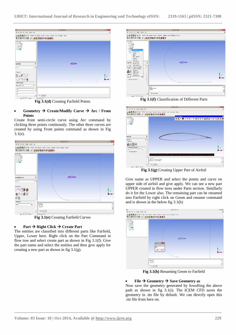
Fig 3.1(d) Creating Farfield Points
Geometry Create/Modify Curve Arc / From
Points
Create front semi-circle curve using Arc command by
clicking three points continously. The other three curves are
created by using From points command as shown in Fig
3.1(e).
Fig 3.1(e) Creating Farfield Curves
Part Right Click Create Part
The entities are classified into different parts like Farfield,
Upper, Lower here. Right click on the Part Command in
flow tree and select create part as shown in Fig 3.1(f). Give
the part name and select the entities and then give apply for
creating a new part as shown in fig 3.1(g).
Fig 3.1(f) Classification of Different Parts
Fig 3.1(g) Creating Upper Part of Airfoil
Give name as UPPER and select the points and curve on
upper side of airfoil and give apply. We can see a new part
UPPER created in flow tress under Parts section. Simillarly
do it for the Lower also. The remaining part can be renamed
into Farfield by right click on Geom and rename command and is shown in the below fig 3.1(h)
Fig 3.1(h) Renaming Geom to Farfield
File Geometry Save Geometry as
Now save the geometry generated by fowolling the above
path as shown in fig 3.1(i). The ICEM CFD saves the
geometry in .tin file by default. We can directly open this
.tin file from here on.
IJRET: International Journal of Research in Engineering and Technology eISSN: 2319-1163 | pISSN: 2321-7308
_______________________________________________________________________________________
Volume: 03 Issue: 10 | Oct-2014, Available @ http://www.ijret.org 230
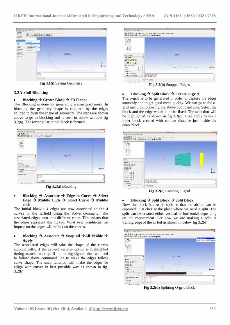
Fig 3.1(i) Saving Geometry
3.2Airfoil Blocking
Blocking Create Block 2D Planar
The Blocking is done for generating a structured mesh. In
blocking the geometry shape is captured by the edges splitted to form the shape of geometry. The steps are shown
above to go to blocking and is seen in below window fig
3.2(a). The rectangular initial block is formed.
Fig 3.2(a) Blocking
Blocking Associate Edge to Curve Select
Edge Middle Click Select Curve Middle
click The initial block‘s 4 edges are now associated to the 4
curves of the farfield using the above command. The
associated edges turn into different color. This means that
the edges represent the curves. What ever conditions we
impose on the edges will reflect on the curves.
Blocking Associate Snap all All Visible
Apply
The associated edges will take the shape of the curves
automatically, if the project vertices option is highlighted
during association step. If its not highlighted then we need to follow above command line to make the edges follow
curve shape. The snap function will make the edges be
allign with curves in best possible way as shown in fig.
3.2(b)
Fig 3.2(b) Snapped Edges
Blocking Split Block Create O-grid
The o-grid is to be generated in order to capture the edges
smoothly and to get good mesh quality. We can go to the o-
grid menu by following the above command line. Select the
block and the edge which is to be fixed. The selection will
be highlighted as shown in fig 3.2(c). Give apply to see a
inner block created with contant distance just inside the
outer block.
Fig 3.2(c) Creating O-grid
Blocking Split Block Split Block
Now the block has to be split so that the airfoil can be
captured. Just click at the place where we need a split. The
split can be created either vertical or horizontal depending
on the requirement. For now we are making a split at trailing edge of the airfoil as shown in below fig 3.2(d)
Fig 3.2(d) Splitting O-grid block

IJRET: International Journal of Research in Engineering and Technology eISSN: 2319-1163 | pISSN: 2321-7308
_______________________________________________________________________________________
Volume: 03 Issue: 10 | Oct-2014, Available @ http://www.ijret.org 231
Blocking Associate Edge to Curve
Now associate the inner block upper edge with upper curve,
inner block lower edge with lower curve and front edge to
both the upper and lower curves as show in below fig 4.2(e).
The Association details can be seen by right clicking on
edge option on flow tree and selecting show association.
Fig 3.2(e) Showing Association of edges to curves
Now the snap all option is used to make the associated
edges take the shape of upper and lower curves. The airfoil
is having a sharp trailing edge. So the other unassociated
edge of the inner block is not necessary. It has to be
collapsed following the below command line to capture the
trailing edge of the airfoil.
Blocking Merge Vertices Collapse Blocks
For collapsing edge first select the edge to be collapsed and
then the block as shown in below fig 4.2(f). Proceed and give apply so that the block will collapse along the edge
length, forming a straight line as shown in below fig 4.2(g)
Fig 3.2(f) Collapsing rear block
Fig 3.2(g) Collapsed block view
The block inside the airfoil should be deleted by using the
following command line. This block should be deleted so
that mesh will be generated, capturing the airfoil curves.
The existing blocks only will get divided into nodes.
Blocking Delete Block Select Block Apply
Blocking Split Block Split Block Create a split in front of the blocking as shown in the below
fig 3.2(h). Create another split so that it will form a c shaped
edge through out the airfoil till the end as shown in fig
3.2(i). These splits will be helpful to improve the quality of
the mesh, which will be discussed later.
Fig 3.2(h) Splitting front block
Fig 3.2(i) Splitting Edges along the Axis

IJRET: International Journal of Research in Engineering and Technology eISSN: 2319-1163 | pISSN: 2321-7308
_______________________________________________________________________________________
Volume: 03 Issue: 10 | Oct-2014, Available @ http://www.ijret.org 232
File Blocking Save Blocking as
Now save the Blocking generated by fowolling the above
path as shown in fig 4.2(j). The ICEM CFD saves the
blocking in .blk file by default. We can directly import this
.blk file for the geometry here on.
Fig 3.2(j) Saving Block
3.3 Edge Parameters
Edge parameters under the blocking menu is used for giving
the number of nodes the edge is to be divided into and
which bunching law it has to follow while dividing the
edge.
Blocking Pre-mesh params Edge Params
Select the edge and give the number of the nodes it has to be
divided into as shown inbelow window fig 3.3(a). We can
also select the type of bunching law it has to follow like
uniform, geometri 1, geometri 2, etc… from the drop down
menu. Simillarly give the edge parameters for all the edges and apply.
Fig 3.3(a) Giving Edge parameters
After giving the edge parameters, in the flow tree, right
click on the pre-mesh under blocking and click on the re-compute and give apply. Now we can see the mesh
generated on the screen as shown in below figure 3.3(b)
Fig 3.3(b) Mesh generated on Airfoil
Now the mesh is generated on the geometry. To go ahead,
the quality of the mesh is to be checked. The ICEM CFD
offers a variety of quality parameters to check mesh quality,
in the drop down menu of quality criterion. Generally we
check Angle and Determinant. The quality options can be seen by going through following command line.
Blocking Pre-mesh Quality Quality
The Drop down menu of the quality criterion under the pre-
mesh quality is shown in below window fig 3.3(c). The
quality criterion Angle of the mesh is checked and found to
be good. The Angle criterion mesh check result is shown in
below fig 3.3(d).
Fig 3.3(c) Premesh Quality checking
Fig 3.3(d) Premesh Quality criterion ANGLE
IJRET: International Journal of Research in Engineering and Technology eISSN: 2319-1163 | pISSN: 2321-7308
_______________________________________________________________________________________
Volume: 03 Issue: 10 | Oct-2014, Available @ http://www.ijret.org 233
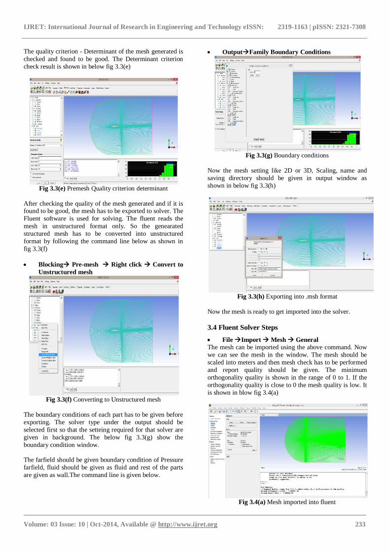
The quality criterion - Determinant of the mesh generated is
checked and found to be good. The Determinant criterion
check result is shown in below fig 3.3(e)
Fig 3.3(e) Premesh Quality criterion determinant
After checking the quality of the mesh generated and if it is found to be good, the mesh has to be exported to solver. The
Fluent software is used for solving. The fluent reads the
mesh in unstructured format only. So the genearated
structured mesh has to be converted into unstructured
format by following the command line below as shown in
fig 3.3(f)
Blocking Pre-mesh Right click Convert to
Unstructured mesh
Fig 3.3(f) Converting to Unstructured mesh
The boundary conditions of each part has to be given before
exporting. The solver type under the output should be
selected first so that the setteing required for that solver are
given in background. The below fig 3.3(g) show the
boundary condition window.
The farfield should be given boundary condition of Pressure
farfield, fluid should be given as fluid and rest of the parts
are given as wall.The command line is given below.
OutputFamily Boundary Conditions
Fig 3.3(g) Boundary conditions
Now the mesh setting like 2D or 3D, Scaling, name and
saving directory should be given in output window as
shown in below fig 3.3(h)
Fig 3.3(h) Exporting into .msh format
Now the mesh is ready to get imported into the solver.
3.4 Fluent Solver Steps
File Import Mesh General
The mesh can be imported using the above command. Now
we can see the mesh in the window. The mesh should be
scaled into meters and then mesh check has to be performed
and report quality should be given. The minimum
orthogonality quality is shown in the range of 0 to 1. If the
orthogonality quality is close to 0 the mesh quality is low. It
is shown in blow fig 3.4(a)
Fig 3.4(a) Mesh imported into fluent

IJRET: International Journal of Research in Engineering and Technology eISSN: 2319-1163 | pISSN: 2321-7308
_______________________________________________________________________________________
Volume: 03 Issue: 10 | Oct-2014, Available @ http://www.ijret.org 234
The solver settings should be given now. The Density based
solver is choosed and the other parameters are given as
shown in below fig 3.4(b)
Fig 3.4(b) Mesh checked.
Model Energy Equation On
Model Viscous Kω-SST Apply
Material Fluid Air Ideal gas Apply
Cell Zone Conditions Operating Pressure 0
Pa Apply
Boundary Conditions Check Farfield Condition Edit
The run conditions menu is seen by upper command line
and run conditions are given as shown in below fig 3.4(c).
The gauge pressure, mach, temperature and angle of attack
values should be given. The gauge pressure is calculated with respect to the indian standard atmosphere.
Fig 3.4(c) Simulation conditions
Reference Values Compute from Farfield(ff)
Give the values of aera of the geometry and the reference
length. The remaining values are calculated automatically from previous data. The window is shown in below fig
3.4(d)
Fig 3.4(d) Reference values
Solution Method Formulation Implicit
Solution Method Flux type Roe-FDS
Solution Method Gradient Green-Gauss Cell
Based
The solution method window is shown in below fig 3.4(e).
The above command options are selected from the drop
down menus as shown in figure. The flow order is to be
choosed according to the requirement of the simulation.
Fig 3.4(e) Solution methods
Solution Controls Courant Number
2.5(default)
The courant number will have a high impact on the
convergence of the simulation. The courant number should
be given considering the mach number and the mesh quality for the simulation. The courant number should be reduced
with increase in the mach number value. The courant
number window is shown in below fig 3.4(f)
Fig 3.4(f) Solution controls
IJRET: International Journal of Research in Engineering and Technology eISSN: 2319-1163 | pISSN: 2321-7308
_______________________________________________________________________________________
Volume: 03 Issue: 10 | Oct-2014, Available @ http://www.ijret.org 235
Monitors Residuals Print, Plot, Write
Monitors Cl Upper, Lower Print, Plot,
Write
Monitors Cd Upper, Lower Print, Plot,
Write
Monitors Cm Upper, Lower Print, Plot,
Write
The monitors are important to see the convergence of the
simulation. The monitors can be seen as plots with respect
to iterations and they can also be written to a file and saved.
Fig 3.4(g) Simulation monitors
Solution Initialization Standard Intialization
Compute from farfield Initialize
For any simulation the initialization should be done after
giving all the setting and method of solving before
calculating the solution.
Fig 3.4(h) Simulation intialization
Run Calculations Iterations 1000 Run
We can automatically save the simulation results by using
the calculation activities in the flow tree. Otherwise we can
save them manually using save case and that under the file
menu. The case file will have the geometry details and the
dat file will have all the simulation data. The result of the
simulation can be seen through report and force report. The
axial, normal forces and coefficients are obtained from the
force report files which in return help to calculate the Lift
and Drag.
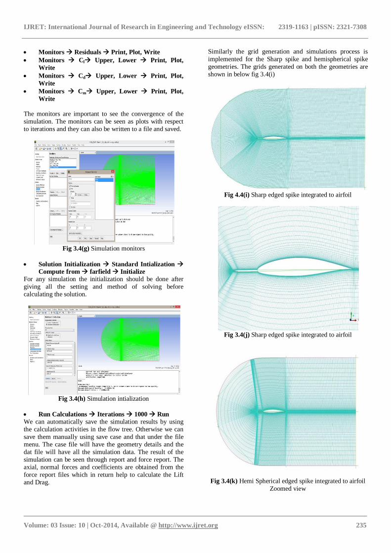
Similarly the grid generation and simulations process is
implemented for the Sharp spike and hemispherical spike
geometries. The grids generated on both the geometries are
shown in below fig 3.4(i)
Fig 4.4(i) Sharp edged spike integrated to airfoil
Fig 3.4(j) Sharp edged spike integrated to airfoil
Fig 3.4(k) Hemi Spherical edged spike integrated to airfoil
Zoomed view

IJRET: International Journal of Research in Engineering and Technology eISSN: 2319-1163 | pISSN: 2321-7308
_______________________________________________________________________________________
Volume: 03 Issue: 10 | Oct-2014, Available @ http://www.ijret.org 236
Fig 3.4(l) Hemi Spherical edged spike integrated to airfoil
Zoomed vie
4. RESULTS
4.1 Contours
These are the Contours resulted after completion of
simulation process in ANSYS Fluent.
Fig 4.1(a) Pressure Coefficient contour over NACA 651-
412
Fig 4.1(b) Pressure Coefficient contour over NACA 651-
412 zoomed view
Fig 4.1(c) Pressure Coefficient contour over sharp spike
integrated airfoil
Fig 4.1(d): Velocity Magnitude Contour over sharp spike
integrated airfoil
Fig 4.1(e): Velocity Vector of Velocity Magnitudeover
sharp spike integrated airfoil

IJRET: International Journal of Research in Engineering and Technology eISSN: 2319-1163 | pISSN: 2321-7308
_______________________________________________________________________________________
Volume: 03 Issue: 10 | Oct-2014, Available @ http://www.ijret.org 237
Fig 4.1(f): Pressure Coefficient contour over hemispherical
spike integrated airfoil
Fig 4.1(g): Velocity Magnitude Contour over hemispherical
spike integrated airfoil
Fig 4.1(h): Velocity Vector of Velocity Magnitudeover
hemispherical spike integrated airfoil
Fig 4.1(i): Velocity Vector of Velocity Magnitude over
hemispherical spike integrated airfoil zoomed view
5. CONVERGENCE
The simulations were run until the converged solution is
obtained. The convergence plot shows the simulation
convergence. The convergence plot is obtained by plotting
the iterations with respect to coefficient. The convergence
plots of the NACA 651-412 simulation are shown in below fig 5.1 and fig 5.2
Fig 5.1 Lift Convergence
Fig 5.2 Drag Convergence

IJRET: International Journal of Research in Engineering and Technology eISSN: 2319-1163 | pISSN: 2321-7308
_______________________________________________________________________________________
Volume: 03 Issue: 10 | Oct-2014, Available @ http://www.ijret.org 238
Calculations
The Axial and Normal Forces and coefficients are obtained
from the simulation results through force report files. These
values are now used to calculate the lift and drag generated
due to the supersonic flow over the airfoils. The comparison
is made between the normal airfoil and two airfoils with
spikes to see the change in the lift and drag forces, i.e. the aerodynamic loads. The force value of the sharp spike is
also compared with the hemispherical one to find the effect
of shape of spike on the aerodynamic loads. The formula
used for the calculations and the calculated values are
shown below
Drag (D) = 𝑁 ∗ sin 𝛼 + 𝐴 ∗ cos(𝛼) Where, N = Normal Force,
A = Axial Force,
α = Angle of attack
Table: Calculation
6. DISCUSSION
Experiments have been made to visualize the overall flow field over NACA 651-412 aerofoil with and without spike.
The simulation velocity contours pictures shown indicate a
strong detached bow shock wave in front of NACA 6 series
aerofoil as expected. With adoption of sharp spike, a conical
shock is observed and with hemi spherical spike, a bow
shock is observed. The closer look of velocity vector on all
the cases studied, the flow is reversed. The measured drag
(CD) for NACA 6 series aerofoil with adoption of sharp
spike is much decreased than hemi spherical spike adopted
case. This indicates that, use of any of these spikes lead to
substantial reduction in drag.
The pressure contours for all the cases are shown in fig.3
along with typical values of pressure. Pressure is observed
to be maximum at Leading edge of NACA 6 series aerofoil.
For sharp spike case, low pressure effect is observed on
spike as well as on NACA 6 series aerofoil. But in hemi
spherical case, pressure values too high at head of hemi
spherical spike as well as at Leading edge of aerofoil.
The main reduction in drag is due to reduction in pressure
drag on the aerofoil with change in spike. This indicates that
the further reduction in drag could be achieved by suitably modifying the sharp spike mainly and as well as hemi
spherical tip of spike.
7. CONCLUSION AND FUTURE SCOPE
Computations have been made to obtain the flow field on a
NACA 651-412 aerofoil at a supersonic Mach number of 2,
in the presence of a sharp spike and hemi spherical head
spike. It was observed that in general the drag reduces.
Computations results indicate more details of flow field and
effect of spike shape and its length with and without spike mode.
Estimation of drag for different components indicate that
major reduction is from the NACA 6 series aerofoil which
get modified due to spike tip and hence shape and size of
spike is of prime importance for reduction of drag.
FUTURE SCOPE OF WORK
To implement the spike to 3D wing geometry and
study the effect of spike on the complete wing.
To implement the spike to supersonic aircraft wings
and compare its effect.
To increase the performance of aircraft by making it capable to fly in both subsonic and supersonic flight
speeds
To reduce the fuel usage in supersonic aircraft
REFERENCES
[1]. P.k.kundu, I.M.cohen. Fluid Mechanics 3/e. Academic
press, Indian Reprint 2005.
[2]. Kalimuthu, r. and Rathakrishnan, E., ―Aerospike for
drag reduction in hypersonic flow‖, AIAA-2008-4707.
[3]. Kalimuthu,R., Mehta, R.C. and Rathakrishnan, E.,
―Drag Reduction for Spike Attached to Blunt-nosed Body at
Mach 6‖, Engineering Notes, Journal of Spacecraft and
Rockets, Vol.47, No.1, jan-Feb,2010,pp.219-222. [4]. D‘Humieres, G. and Stollery, J.l., ―Drag Reduction on a
Spiked Body at Hypersonic Speed‖, The Aeronautical
Journal, Paper No.3482, Vol.114, No.1152, February, 2010,
pp.113-119.
[5]. Ahmed, M.Y.M. and Qin, N., ―Recent Advances in the
Aerothermodynamics of Spiked Hypersonic vehicles‖,
Progress in Aerospace Sciences, 47, 2011, pp.425-449.
[6]. Van Driest, E.R.: ―The Problem of Aerodynamic
Heating‖, Aeronautical Engineering Review, Oct. 1956, pp.
26-41.
[7]. Anderson, John D., Jr., Fundamentals of Aerodynamics,
3rd edi., McGraw-Hill Book Company, New York, 1984.
Force
Normal
Airfoil
Sharp
Spike
Hemispherical
spike
Axial Force 22755.33 16761.71 19744.23
Normal
Force -8961.96 11077.2 9497.34
Drag (at α =
00) 22755.33 16761.71 19744.23
Coefficient
of Drag 0.080994 0.059608 0.070214