HAL Id: hal-02923929https://hal.archives-ouvertes.fr/hal-02923929

Submitted on 6 Jan 2021

HAL is a multi-disciplinary open accessarchive for the deposit and dissemination of sci-entific research documents, whether they are pub-lished or not. The documents may come fromteaching and research institutions in France orabroad, or from public or private research centers.

L’archive ouverte pluridisciplinaire HAL, estdestinée au dépôt et à la diffusion de documentsscientifiques de niveau recherche, publiés ou non,émanant des établissements d’enseignement et derecherche français ou étrangers, des laboratoirespublics ou privés.

Effect of Roll Motion Control on Vehicle LateralStability and Rollover Avoidance

Abbas Chokor, Reine Talj, Moustapha Doumiati, Ali Charara

To cite this version:Abbas Chokor, Reine Talj, Moustapha Doumiati, Ali Charara. Effect of Roll Motion Control onVehicle Lateral Stability and Rollover Avoidance. American Control Conference (ACC 2020), Jul2020, Denver, United States. pp.4868-4875, �10.23919/ACC45564.2020.9147735�. �hal-02923929�

Effect of Roll Motion Control on Vehicle Lateral Stability and RolloverAvoidance *

Abbas Chokor, Reine Talj, Moustapha Doumiati and Ali Charara

Abstract— This paper discusses the effects of the roll controlon the vehicle performance. Rollover avoidance and lateralstability constitute the core analysis of this paper. Two rollreference generators, one static (towards zero) and one dynamic(function of the vehicle lateral acceleration) are designed forcontrol purpose. Roll motion control is achieved through thegeneration of a feedback roll moment. To track the staticroll reference, the roll moment can be allocated to the activesuspensions, the semi-active suspensions, or the active anti-roll bar, while the roll motion control towards the dynamicreference can be only achieved using the active suspensions. Todo so, firstly, based on the time-domain equations of motionof the full-vehicle nonlinear model, a study on how the rollcontrol can help the vehicle to avoid the rollover withoutdeceleration or steering actions is done. Secondly, a frequencyanalysis of the lateral stability response to the steering input,with and without roll motion control is performed to extractthe ranges of steering frequencies and amplitudes where theroll control could be useful. For this study, two lateral-rolllinear time invariant vehicle models (without and with linearquadratic roll control) are compared. Thirdly, two robust rollcontrollers, i.e., Lyapunov-based, and super-twisting slidingmode are developed, validated and compared on the fullvehicle nonlinear model using Matlab/Simulink. This paper alsoprovides a comparison between the roll angle control towardsthe static and the dynamic references.

I. INTRODUCTION

Driving safety is a major challenge where rollover andlateral skidding commit the major fatal injuries [1], [2]. Theeffect of the roll motion control on the rollover phenomenonis obvious since it is effected by the lateral acceleration.The vehicle rollover has been treated by several AdvancedDriving Assistance Systems (ADAS), either by braking orsteering [3], [4], or in a Global Chassis Control (GCC)architectures [5], [6], [7] where the authors propose DirectYaw Controllers (DYC) that has the desired yaw rate toswitch between two expressions, one is to enhance the lateralstability and the other one is to avoid rollover. However, thesesystems have the disadvantage of decelerating the vehicle.Authors in [5] have shown a better performance by achievingthe same DYC objective through the Active DifferentialBraking (ADB). Some other relevant research such as [3],[4] propose to control the roll motion by the Active FrontSteering (AFS) and/or ADB to avoid the rollover, regardlessof the vehicle maneuverability and trajectory.

* This work was supported by the Hauts-de-France Region and theEuropean Regional Development Fund (ERDF).

A. Chokor, R. Talj and A. Charara are with Sorbonne universites,Universite de Technologie de Compiegne, CNRS, Heudiasyc UMR 7253,CS 60 319, 60 203 Compiegne, France.

M. Doumiati is with ESEO-IREENA EA 4642, 10 Bd Jeanneteau, 49100Angers, France.

The effect of the roll motion control on the lateral stabilityis more complicated. The dynamics coupling between thevertical and lateral tire forces is an essential key to enhancethe lateral stability [8]. Several studies on the (semi-)ActiveSuspensions (ASus) are conducted to explicitly try to enhancethe lateral stability [9], [10]. The basic idea is to preventthe saturation of tires lateral forces. For that, researchersas in [12], [13], [14] propose to control the vertical loadtransfer when cornering. However, this method may ensurea posterior enhancement on the lateral stability but not aprior demonstrated guaranty. One of this paper objectives isto demonstrate, a priori, in the frequency domain, that theroll angle control can always enhance the lateral stability.Therefrom, the noticed enhancements in these different GCCapproaches have motivated us to create a new synergyrepresented by achieving the rollover avoidance and thelateral stability objectives through the ASus, usually used forride comfort and road holding.The main contributions of this paper are:

• a time-domain analysis of the effect of the roll motioncontrol on the rollover avoidance;

• a frequency-domain analysis of the effect of the rollmotion control on the lateral stability;

• development and comparison between a LinearQuadratic Regulator (LQR), a Lyapunov-based, and aSuper-Twisting Sliding Mode (ST SM) controllers tocontrol the roll motion;

• a comparison between the roll angle control towardsthe static reference zero and the new desired roll angle(dynamic reference).

The paper structure is as follows: Section II provides anonlinear representation of the vehicle roll motion dynamics,followed by a linear vehicle model called extended bicyclemodel. Section III and IV expose the roll control effect onrollover and lateral stability problems. Section V presents thegeneral closed loop architecture, including the reference gen-erator, the controllers and the actuators. Section VI exposesthe Lyapunov-based and the ST SM controllers. In SectionVII, the proposed controllers are validated by simulation.Finally, Section VIII concludes the achievements of this workand provides a glance about future contributions.

II. VEHICLE DYNAMICS

A full vehicle model has been already developed andvalidated using “SCANeR Studio Simulator” [15], [16]. Thefull vehicle model serves here to validate the roll motion con-trollers. From the full vehicle model, the dynamic equation

2020 American Control ConferenceDenver, CO, USA, July 1-3, 2020

978-1-5386-8266-1/$31.00 ©2020 AACC 4868

Authorized licensed use limited to: Universite de Technologie de Compiegne (UTC). Downloaded on December 18,2020 at 13:37:31 UTC from IEEE Xplore. Restrictions apply.

CG

zsM s .a y

M s .ghθ

F fr+Frr F fl+F rl

θ

F z , fr+F z ,rr F z , fl+F z , rl

Mθ

Fig. 1: roll motion (front view)

of the sprung mass roll motion is modeled as:

θ =1

Ix +Msh2θ

[(−Ff r +Ff l

)t f +(−Frr +Frl) tr

+Ms (hθ cos(θ)+ zs)ay +Ms (hθ sin(θ)+ zs)g+Mθ ],

(1)

as shown in Fig. 1, where, Ms, hθ and hφ are respectivelythe sprung mass weight, the distance between the center ofgravity of the sprung mass and the roll rotation center, andthe distance between the center of gravity of the sprung massand the pitch rotation center. Ix is the moment of inertia ofthe sprung mass around the x axis. ay is the vehicle lateralacceleration, considered as exogenous inputs to this equation.Mθ is the active roll moment to be generated through theASus forces, and Fi j is the passive suspension force on thevehicle corner i j (i= { f : f ront,r : rear} and j = {r : right, l :le f t}), such as:

Fi j =−Ks,i j(zs,i j− zus,i j)−Cs,i j(zs,i j− zus,i j), (2)

where Ks,i j, and Cs,i j are respectively the suspension stiffnesscoefficient and the suspension damping coefficient. zs,i j andzus,i j are respectively the vertical displacement of the sprungmass and the unsprung mass (wheel bounce), considered asexogenous inputs to this equation.

From the other side, the extended bicycle model is acoupled lateral-roll vehicle model. It is a linear simplifiedvehicle model which combines the vehicle yaw and side-slipto the roll motion. This model is suitable to analyze theeffect of the roll motion control on the lateral stability ofthe vehicle. The extended bicycle model is inspired fromliterature [12] as the following:

Izψ = Fy f l f +Fyrlr + Ixzθ ,

MV(

β + ψ

)= Fy f +Fyr +Mshθ θ ,(

Ix +Msh2θ

)θ = MshθV

(β + ψ

)+(Msghθ −Kθ )θ −Cθ θ +Mθ ,

(3)where Fy f and Fyr respectively represent the lateral force ofthe tire on the front axle and on the rear axle; Mθ representsthe active roll moment as a control input. Fy f and Fyr aresupposed to be linear to the wheels side-slip angle such that:

Fy f = µC f α f ,Fyr = µCrαr,

(4)

where C f and Cr are respectively the double of the front andrear tires cornering stiffness. The wheels side-slip angles arefound using the following equations:

α f =−β − l f ψ

V +δ f ,

αr =−β + lrψ

V .(5)

˙ψ

β

θ

θ

=

a11 a12 a13 a14a21 a22 a23 a240 0 0 1

a41 a42 a43 a44

︸ ︷︷ ︸

A

ψ

β

θ

θ

︸︷︷ ︸

X

+

bu,11 bu,12bu,21 bu,22

0 0bu,41 bu,42

︸ ︷︷ ︸

B

[δdMθ

]

(6)As can be seen, the extended bicycle model is an improvedversion of the bicycle model where firstly the roll dynamicsis described by a linear differential equation and secondly itis included into the lateral motion equations. By substituting(5) in (4), and then in (3), the state space representationof the extended bicycle model can be formalized as in (6),where X = [ψ,β ,θ , θ ]T is the state vector. The elements ofthe state matrix A ∈ IR4×4, and the input matrix B ∈ IR4×2

are formalized in Appendix I.

III. ROLL MOTION EFFECT ON ROLLOVER PROBLEM

To study the motion roll effect on rollover, suppose thatthe vehicle has one degree of freedom represented by the rollangle θ between the suspended and unsuspended masses (seeFig. 1). This means that the suspended mass center of gravitydeviates by a positive angle θ (toward the outside) aroundthe roll axis. Hereby, the moment of all forces around theaxis joining outer wheels becomes:

Msayh−Msg(t f − (h−hr)sinθ)+Fzi2t f = 0. (7)

where Fzi is the vertical force representing the summationof the front and rear vertical forces of the inner ( w.r.t thecorner) wheels, and t f is the vehicle half track. Because ofthe equilibrium of (7), if ay increases, a natural decreasing ofthe other single variable Fzi happens, up to a certain amountof ay where Fzi becomes 0, which represents inner wheelslift-off. Under the assumption of small angles sinθ ≈ θ , thelateral acceleration that causes wheels lift-off is:

ay,li f t−o f f =t f − (h−hr)θ

hg, (8)

In order to stay in a safe driving region, a safety factor of0.7 of the total ay,li f t−o f f expressed in (8) is proposed, suchas:

ay,sa f e = 0.7ay,li f t−o f f = 0.7t f − (h−hr)θ

hg (9)

To avoid the rollover, ay should be maintained below aysa f e .While several control actions like the AFS and the ADBaim to reduce ay, the ASus, semi-ASus and the Active anti-Roll Bar (ARB) aim, by controlling the roll angle, to elevatethe maximal safe lateral acceleration ay,sa f e. For instance,stiffening the suspensions using the semi-ASus or the ARBcan reduce the vehicle roll angle towards zero which arisesay,sa f e as exhibits equation (9). The contribution that adds theASus system is the ability to continue turning the roll anglein the negative direction (to the inner side of the corner),that means ay,sa f e will be more shifted to a higher value.The choice of the desired roll angle θdes is done as follows:- At zero lateral acceleration (straight road), the desired rollangle is 0◦.- At a lateral acceleration equal to the maximal static safelateral acceleration threshold 0.7 t f

h g, the desired roll angle

4869

Authorized licensed use limited to: Universite de Technologie de Compiegne (UTC). Downloaded on December 18,2020 at 13:37:31 UTC from IEEE Xplore. Restrictions apply.

is equal to the maximal achievable roll angle 10◦ (vehicledesign constraints) [17].- The map between θdes and ay is supposed to be linearto make a smooth comfortable roll change rate. Thus, thedesired roll angle θdes is given as:

θdes =−10 π

180

0.7 t fh g

ay. (10)

IV. ROLL CONTROL EFFECT ON LATERAL STABILITY

A. Stability Index SI Criterion

The most known criterion to evaluate the lateral stabilityis called “Stability Index” (SI) [18], [19], [20]. SI can beexpressed as:

SI =∣∣∣q1β +q2β

∣∣∣ , (11)

where q1 and q2 are identified depending on the vehicleparameters and road adherence µ to characterize the stableboundary of the β − β phase plane. SI is normalized andvaries between 0 and 1. For SI ≤ SI (a predefined lowerthreshold depending on the vehicle and road parameters),the vehicle is in normal driving situations (stable region); upto a predefined higher threshold SI, the vehicle is consideredin the critical lateral stability region, where active safetycontrollers have to be triggered to cover back the lateralstability of the vehicle; beyond SI the vehicle operates inthe unstable region.

B. Frequency Analysis Setup

The relation between the roll angle θ and the lateralstability quantified by the SI criterion (β − β ) is governedby the dynamical system given in (6). Therefore, this sectionanalyzes, in the frequency and time domains, the effect ofthe roll control on the lateral stability.The LT I model (6) can be written as:

X = AX +B1δd +B2Mθ , (12)

where B1 and B2 are respectively the first and second columnof B.The objective is to compare the frequency response of thevehicle with a controlled roll motion as in (12), and thevehicle without a roll controller (Mθ = 0) as in (13):

X = AX +B1δd . (13)

Thus, let consider the state feedback LQR control law:

Mθ =−KX . (14)

The optimal closed-loop system becomes:

X = (A−B2K)X +B1δd , (15)

which has the same form as (13), but with a controlled rollmotion.The optimization procedure consists in finding the controlinput U = Mθ which minimizes the performance index J:

J =∫

∞

0(XT QX +UT RU)dt, (16)

10-1

100

101

102

103

104

Mag

nitu

de M

(dB)

14

15

16

17

18

19

20

21

22Without roll control

With roll control

SI/delta

Frequency ω (rad/s)

Fig. 2: Bode plot SI/δd ; V = 100 km/h

where Q and R are the weighting matrices.The control purpose is to minimize the roll angle and rollvelocity, by controlling Mθ . Thus, the performance index Jbecomes:

J =∫

∞

0(ρ1θ

2 +ρ2θ2 +M2

θ )dt, (17)

where the weighting coefficients ρ1 and ρ2 are adjusted topromote the weight on the roll angle and its rate of change,while minimizing the energy of the control input.The matrix gain K has the form:

K = R−1BT2 P, (18)

where the matrix P is the solution of the Algebric RiccatiEquation:

AT P+PA−PB2R−1BT2 P+Q = 0. (19)

The frequency response of the vehicle with roll controller(15) and the vehicle without roll controller (13) can be nowcompared.

C. Lateral Stability Frequency Analysis

To analyze the frequency response of the vehicle lateralstability w.r.t the driver steering input, the transfer functionsGSI

δdof both uncontrolled (13) and controlled (15) LT I

systems are evaluated in Matlab environment, and their bodediagrams at the vehicle speed V = 100 km/h are plotted inFig. 2. Both curves in Fig. 2 represent the magnitude M(ω)of GSI

δdin (db) over the frequency range ω of δd .

The magnitude response of GSIδd

of the uncontrolled rollvehicle increases significantly, while controlling the rollangle remarkably reduces the response of GSI

δ, especially

at frequencies around the peak magnitude. Based on thefollowing relation,

SI = A∗10M(ω)

20 , (20)

at a high steering amplitude (A > 0.1 rad), the SI of theuncontrolled roll vehicle exceeds SI = 1, while the controlledone establishes acceptable behavior.In order to generalize for any speed, the frequency responses

GSIδd

of the controlled and uncontrolled vehicles are evaluatedat different speeds V = 70, 85, 100, 115 km/h. The resultsare illustrated in Fig. 3. This figure shows that as muchas the speed becomes higher, as the difference betweenthe magnitude curves (at the same speed) becomes greater.

4870

Authorized licensed use limited to: Universite de Technologie de Compiegne (UTC). Downloaded on December 18,2020 at 13:37:31 UTC from IEEE Xplore. Restrictions apply.

10-1

100

101

102

103

104

Mag

nitu

de M

(dB)

5

10

15

20

25

Without roll control

With roll control

SI/delta

Frequency ω (rad/s)

V=70 km/h

V=115 km/h

V=100 km/h V=115 km/h

V=100 km/h

V=85 km/h

V=70 km/h

V=85 km/h

Fig. 3: Bode plot SI/δd

Full vehicle

model Roll reference

generator

0

Roll

controllerAllocation

unitActuators

Driver

θ

ay

θ

θdes

Uij x 4Mθ

U*ij x 4

ay

δ

θdes

Switch

Torques(driving+braking)

Fig. 4: Control scheme

Hence, at high speed, the roll motion control becomes moreinfluencing on the lateral stability enhancement.

V. CLOSED-LOOP CONTROL ARCHITECTURE

Based on the previous analysis, this section presents thegeneral closed-loop control scheme to be developed as shownin Fig. 4. The roll reference generator block is either staticat zero or dynamic as in (10). The roll controller blockis one of the three control techniques: Linear QuadraticRegulation LQR, Lyapunov-based, and ST SM that will bedeveloped in the next section. The control input Mθ has tobe generated by the actuators forces or torques dependingon the integrated technology. An example (but not restrictedto) is the distribution of Mθ between the four active forcesUi j of the ASus. This is done in the control allocation unitas described in (21):

U f l = 0.5 lrl f +lr

Mθ

t f; U f r =−0.5 lr

l f +lrMθ

t f;

Url = 0.5 l fl f +lr

Mθ

tr; Urr =−0.5 l f

l f +lrMθ

tr.

(21)

The choice of this distribution is done in order to avoid anyinfluence on the pitch angle and the bounce displacementas shown in Fig. 5.

Fig. 5: Active forces distribution

VI. ROLL MOTION CONTROLLERS DESIGN

This section is dedicated to design robust controllersfor the roll motion. The Lyapunov-based control techniqueand the ST SM control technique are used to develop theroll motion controllers. These robust control techniques arechosen to deal with the nonlinear behavior/dynamics of thevehicle. A performance comparison between the Lyapunov-based, the ST SM, and the LQR controllers is also performed.As discussed before, the objectives of these controllers areeither to converge the nonlinear roll motion θ given in (1)to zero or to θdes given in (10). The controllers will bedeveloped for a general reference θdes of θ , then, they willbe tested for both references.Let first define:

eθ = θ −θdes, (22)

the error between the actual and desired roll angles.

A. Lyapunov-Based Controller

The control objective is to converge the roll error variableeθ (of relative degree 2 w.r.t the control input Mθ ) to zero.Let define the “off-the-manifold” variable zθ , such as:

zθ = eθ + k1θ eθ + k2θ

∫ t

0eθ dτ. (23)

Based on Immersion and Invariance approach [21], the “off-the-manifold” variable zθ has to converge to the targetdynamics corresponding to zθ = 0 in the manifold, wherethe roll error dynamics obey to the following equation:

eθ + k1θ eθ + k2θ

∫ t

0eθ dτ = 0, (24)

where k1θ> 0 and k2θ> 0 (Routh-Hurwitz stability conditionfor a second order characteristic polynomial). Despite thefact that the convergence of

∫ t0 eθ dτ to zero is not a necessary

condition, its addition helps to reduce the permanent steady-state error.In order to render the manifold attractive, let define a positivedefinite Lyapunov candidate function as follows:

Vθ =12

zθ2, (25)

Vθ should be negative (Lyapunov stability conditions), thus,

Vθ = zθ zθ ≤ 0, (26)

then, in order to ensure an exponential convergence of zθ tozero, let:

zθ =−αθ zθ , (27)

which makes (26) always negative if αθ > 0. Thus:

eθ +k1θ eθ +k2θ eθ =−αθ (eθ +k1θ eθ +k2θ

∫ t

0eθ dτ), (28)

whereeθ = θ − θdes, (29)

4871

Authorized licensed use limited to: Universite de Technologie de Compiegne (UTC). Downloaded on December 18,2020 at 13:37:31 UTC from IEEE Xplore. Restrictions apply.

then substituting θ from (1) in (28), the control input Mθ

can be found as in (30):

Mθ =(Ix +Msh2θ )[−Mθeq + θdes− (αθ + k1θ )(θ − θdes)

− (αθ k1θ + k2θ )(θ −θdes)−αθ k2θ

∫ t

0(θ −θdes)dτ],

(30)

where

Mθeq =1

Ix +Msh2θ

[(−Ff r +Ff l)t f +(−Frr +Frl)tr

+Ms(hθ cos(θ)+ zs)ay +Ms(hθ sin(θ)+ zs)g].(31)

This control input means that the vehicle parameters shouldbe well estimated and several variables need to be measuredor estimated. Indeed, −Mθeq and (Ix +Msh2

θ) compensate all

the dynamics of the roll angle expressed in (1) as a feedfor-ward command, beside the robust terms of the feedback oneθ , its time derivative and integral of equation (30). θ , θ ,and ay, zs are measured by the Inertial Measurement UnitIMU, the suspension forces Fi j could be estimated fromsuspensions’ deflections.

B. Super-Twisting Second Order Sliding Mode Controller

A second controller has been developed based on theST SM technique. The Super-Twisting algorithm is a secondorder sliding mode control that handles a relative degreeequal to one [22]. It generates the continuous control functionthat drives the sliding variable and its derivative to zero infinite time in the presence of smooth matched disturbances.Let define the sliding variable as follows:

sθ = eθ + kθ eθ , (32)

where kθ> 0. Unlike the preceding Lyapunov controller,the integral term of eθ has not been considered inside thevariable sθ , because the super-twisting algorithm is a secondorder sliding mode, it contains an integral term on the signof sθ [23]. The variable sθ has a relative degree of 1 w.r.tthe control input Mθ , with a second derivative written as:

sθ (sθ , t) = Φ(sθ , t)+ξ (sθ , t)Mθ (t), (33)

where Φ(s, t) and ξ (s, t) are unknown bounded functions.The control objective is to achieve the convergence to thesliding surface defined as sθ = 0. Only the knowledge of sθ

is required in real time.Suppose that there exist positive constants S0, bmin, bmax,C0, Mθ ,max such that for |sθ (t)|< S0, the system satisfies thefollowing conditions: |Mθ (t)| ≤Mθ ,max,

|Φ(sθ , t)|<C0,0 < bmin ≤ |ξ (sθ , t)| ≤ bmax.

(34)

The sliding mode control law, based on the Super-Twistingalgorithm, is given by:

Mθ (t)=Mθ ,1+Mθ ,2

{Mθ ,1 =−αθ |sθ |∇sign(sθ ); ∇ ∈]0, 0.5],Mθ ,2 =−βθ sign(sθ ).

(35)

time (s)

0 2 4 6 8

Fron

t whe

els st

eerin

g an

gle (d

eg)

-8

-6

-4

-2

0

2

4

6

8

Fig. 6: Fishhook steering

time (s)

0 2 4 6 8

Roll (

deg)

-8

-6

-4

-2

0

2

4

6

8Uncontrolled

Controlled Lyapunov

Controlled sliding mode

Controlled LQR

Fig. 7: Roll comparison ; θdes = 0

αθ and βθ are positive gains. The finite time convergence isguaranteed by the following conditions [23]: αθ ≥

√4C0(bmaxβθ+C0)

b2min(bminβθ−C0)

,

βθ > C0bmin

.(36)

The ST SM controller is known for its robustness againstparameters uncertainties and disturbances. It converges to thesliding surface in finite time. Once sθ = 0, the error dynamicsobey to the following equation:

eθ + kθ eθ = 0. (37)

eθ and eθ exponentially converge to zero if kθ > 0, and thestates θ and θ exponentially converge to θdes and θdes. To benoted that the term Mθeq of (31) can be added to the controlinput Mθ , as a feedforward, to achieve a faster convergencetowards the sliding surface.

VII. CONTROLLERS VALIDATION AND PERFORMANCECOMPARISON

In this section, the proposed controllers will be validatedon the simulation model (full vehicle model). To do so, thefishhook maneuver shown in Fig. 6 at an initial speed ofV = 130 km/h is the appropriate test to evaluate both thevehicle rollover risk and the lateral stability.

A. Controllers Validation: static θdes

Lyapunov-based, ST SM and LQR controllers are com-pared in this section to evaluate their performances whenminimizing the roll angle to θdes = 0.Figure 7 shows the roll angle for a vehicle with passivesuspensions (uncontrolled roll) which turns up to 7◦ in bothdirections. All the controllers are efficient to control the rollangle toward zero. As a comparison, beside the robust termsof the feedback (30), the Lyapunov-based controller compen-sates all the dynamics of the roll angle as expressed in (31)to have this performance. That means, in real application,

4872

Authorized licensed use limited to: Universite de Technologie de Compiegne (UTC). Downloaded on December 18,2020 at 13:37:31 UTC from IEEE Xplore. Restrictions apply.

time (s)

0 1 2 3 4 5 6 7 8

Late

ral a

ccel

erat

ion

(m/s

2 )

-10

-5

0

5

10

ay without roll controller

ay with Lyapunov roll controller

ay with sliging mode roll controller

ay with LQR roll controller

ay__safe without roll controller

ay__safe with roll controller

°°

°

°

°

° °

°

°

°

°°

°

°

°

°°

**

*

* * **

*

*

*

*

**

*

*

*

Fig. 8: ay comparison ; θdes = 0

time (s)

0 1 2 3 4 5 6 7 8

Late

ral S

tabi

lity

Inde

x

0

0.2

0.4

0.6

0.8

1

1.2 SI without roll controller

SI with Lyapunov roll controller

SI with sliding mode roll controller

SI with LQR roll controller°

°

°

°°

°

°

°

°

°

°

Fig. 9: SI comparison ; θdes = 0

a strong knowledge (estimation, measurement, parametersexactitude, ideal modeling) on the components of Mθeq isneeded. On the other side, the ST SM controller is efficientin controlling the roll angle by only the generation of thefeedback from the roll angle and velocity (35), with no needto compensate the roll dynamics. The performance of theLQR controller is also acceptable to control the roll angletowards zero.Fig. 8 shows the lateral acceleration of the uncontrolledroll vehicle which is approximately the same for all rollcontrollers. This means that the roll control does not affectthe lateral acceleration to avoid rollover. In fact, the con-troller aims to elevate the maximal safe lateral accelerationexpressed in (9), which depends on the roll angle. As theroll angle is minimized to zero, thus, the maximal safelateral acceleration increases as shown in the same figure.Figure 9 shows the lateral SI of the uncontrolled roll vehiclewhich exceeds 0.7, while the controlled ones (by all theproposed controllers) enhance the lateral stability. Even ifthe enhancement is not sufficient, because the SI remainsabove 0.7, the roll control to zero can be used to help theother controllers (AFS and DYC) to avoid the lateral skiddingin a GCC strategy.

B. Controllers Validation: dynamic θdes

In this section, the controllers performances will be eval-uated when controlling θ to θdes in the opposite directionexpressed in (10).Figure 10 shows the uncontrolled roll angle (same as inFig. 7), the desired one, and the controlled ones. TheLyapunov-based controlled one, and the ST SM controlledone accurately track the desired roll trajectory. The LQRcontroller, as is synthesized to minimize the roll angle tozero, not to minimize the error between the roll angle andits desired trajectory, could not track the desired roll as isshown in the same figure. For this reason, in this subsection,the LQR controller is not compared with the Lyapunov-based

time (s)

0 1 2 3 4 5 6 7 8

Rol

l (de

g)

-10

-5

0

5

10

Desired roll

Uncontrolled

Controlled Lyapunov

Controlled sliding mode

Controlled LQR

Fig. 10: Roll comparison ; θdes opposite direction

time (s)

0 1 2 3 4 5 6 7 8

Late

ral a

ccel

erat

ion

(m/s

2 )

-10

-5

0

5

10

ay without roll controller

ay with Lyapunov roll controller

ay with sliging mode roll controller

ay__safe without roll controller

ay__safe with roll controller

x

x

x

xx

x

x

x

x

x

Fig. 11: ay comparison ; θdes opposite direction

and ST SM controllers.Figure 11 shows the approximately confounded lateral ac-

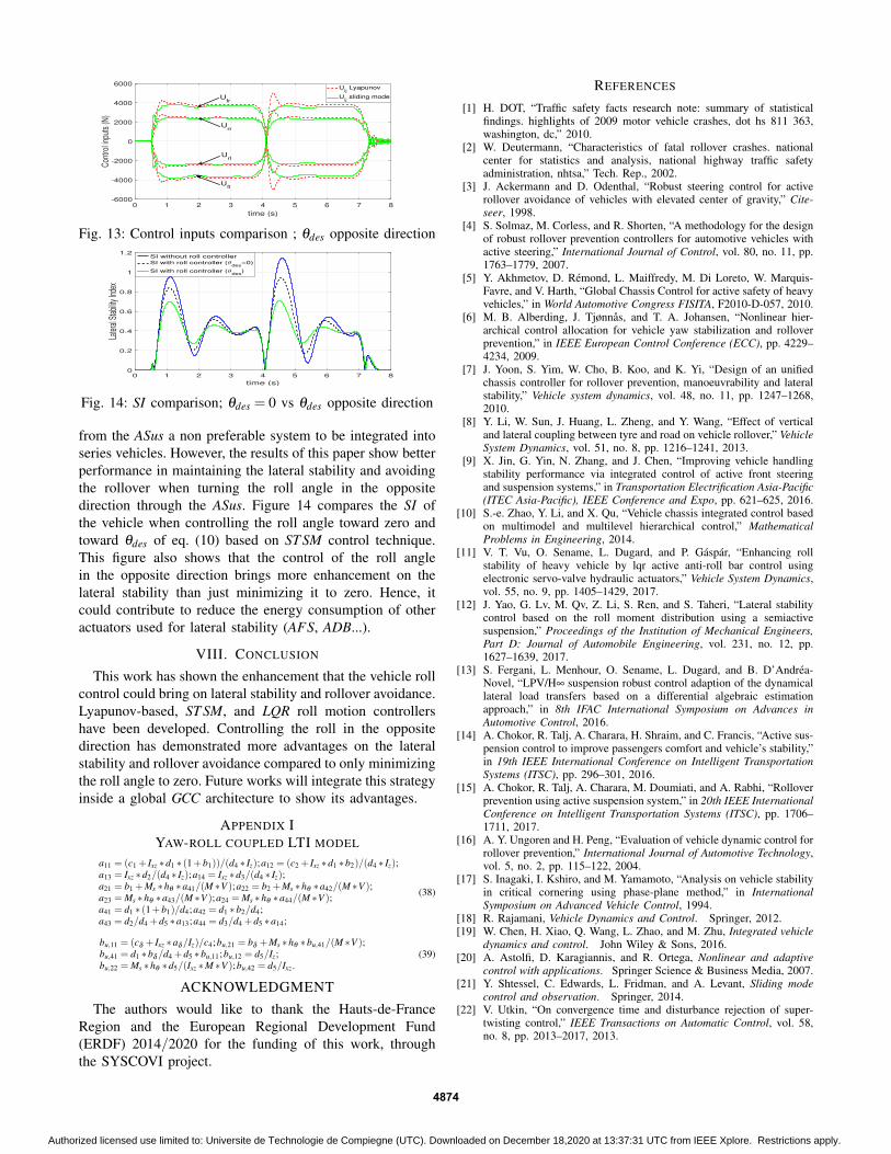
celerations of the uncontrolled roll vehicle, and the controlledones. It also shows the maximal safe lateral accelerationwhich increases more comparing to the case where the rollangle is minimized to zero. This issue drives away therollover risk at this range of lateral acceleration. Figure 12shows the lateral SI of the uncontrolled roll vehicle thatexceeds the value 0.7 up to 1.2 which leads the vehicle toloose its lateral stability. Controlling the roll angle towardthe inside wheels enhances the lateral stability as shown inthe same figure, especially after a sharp steering where theSI is reduced to less than 0.7 by both controllers.Figure 13 shows the control inputs for both Lyapunov-based and sliding mode controllers which are in fact theASus forces provided by the actuators (after saturating andfiltering). This figure shows that their maximal values arearound 4000 N which is feasible by the ASus actuatorswithout any saturation. This fact makes these developedforces realistic and applicable to the vehicle after controllingthe ASus actuators.

C. Roll Reference Performance Comparison

Turning the roll angle in the opposite direction requiresmore energy than just minimizing it to zero, because it canbe only achieved by the ASus which consume more energycomparing to the semi-ASus or the ARB. This fact has made

time (s)

0 1 2 3 4 5 6 7 8

Later

al St

abilit

y Ind

ex

0

0.2

0.4

0.6

0.8

1

1.2SI without roll controller

SI with Lyapunov roll controller

SI with sliding mode roll controller

Fig. 12: SI comparison ; θdes opposite direction4873

Authorized licensed use limited to: Universite de Technologie de Compiegne (UTC). Downloaded on December 18,2020 at 13:37:31 UTC from IEEE Xplore. Restrictions apply.

time (s)

0 1 2 3 4 5 6 7 8

Con

trol i

nput

s (N

)

-6000

-4000

-2000

0

2000

4000

6000U

ij Lyapunov

Uij sliding mode

Url

Urr

Ufr

Ufl

Fig. 13: Control inputs comparison ; θdes opposite direction

time (s)

0 1 2 3 4 5 6 7 8

Late

ral S

tabil

ity In

dex

0

0.2

0.4

0.6

0.8

1

1.2SI without roll controller

SI with roll controller (θdes

=0)

SI with roll controller (θdes

)

Fig. 14: SI comparison; θdes = 0 vs θdes opposite direction

from the ASus a non preferable system to be integrated intoseries vehicles. However, the results of this paper show betterperformance in maintaining the lateral stability and avoidingthe rollover when turning the roll angle in the oppositedirection through the ASus. Figure 14 compares the SI ofthe vehicle when controlling the roll angle toward zero andtoward θdes of eq. (10) based on ST SM control technique.This figure also shows that the control of the roll anglein the opposite direction brings more enhancement on thelateral stability than just minimizing it to zero. Hence, itcould contribute to reduce the energy consumption of otheractuators used for lateral stability (AFS, ADB...).

VIII. CONCLUSION

This work has shown the enhancement that the vehicle rollcontrol could bring on lateral stability and rollover avoidance.Lyapunov-based, ST SM, and LQR roll motion controllershave been developed. Controlling the roll in the oppositedirection has demonstrated more advantages on the lateralstability and rollover avoidance compared to only minimizingthe roll angle to zero. Future works will integrate this strategyinside a global GCC architecture to show its advantages.

APPENDIX IYAW-ROLL COUPLED LTI MODEL

a11 = (c1 + Ixz ∗d1 ∗ (1+b1))/(d4 ∗ Iz);a12 = (c2 + Ixz ∗d1 ∗b2)/(d4 ∗ Iz);a13 = Ixz ∗d2/(d4 ∗ Iz);a14 = Ixz ∗d3/(d4 ∗ Iz);a21 = b1 +Ms ∗hθ ∗a41/(M ∗V );a22 = b2 +Ms ∗hθ ∗a42/(M ∗V );a23 = Ms ∗hθ ∗a43/(M ∗V );a24 = Ms ∗hθ ∗a44/(M ∗V );a41 = d1 ∗ (1+b1)/d4;a42 = d1 ∗b2/d4;a43 = d2/d4 +d5 ∗a13;a44 = d3/d4 +d5 ∗a14;

(38)

bu,11 = (cδ + Ixz ∗aδ /Iz)/c4;bu,21 = bδ +Ms ∗hθ ∗bu,41/(M ∗V );bu,41 = d1 ∗bδ /d4 +d5 ∗bu,11;bu,12 = d5/Iz;bu,22 = Ms ∗hθ ∗d5/(Ixz ∗M ∗V );bu,42 = d5/Ixz.

(39)

ACKNOWLEDGMENT

The authors would like to thank the Hauts-de-FranceRegion and the European Regional Development Fund(ERDF) 2014/2020 for the funding of this work, throughthe SYSCOVI project.

REFERENCES

[1] H. DOT, “Traffic safety facts research note: summary of statisticalfindings. highlights of 2009 motor vehicle crashes, dot hs 811 363,washington, dc,” 2010.

[2] W. Deutermann, “Characteristics of fatal rollover crashes. nationalcenter for statistics and analysis, national highway traffic safetyadministration, nhtsa,” Tech. Rep., 2002.

[3] J. Ackermann and D. Odenthal, “Robust steering control for activerollover avoidance of vehicles with elevated center of gravity,” Cite-seer, 1998.

[4] S. Solmaz, M. Corless, and R. Shorten, “A methodology for the designof robust rollover prevention controllers for automotive vehicles withactive steering,” International Journal of Control, vol. 80, no. 11, pp.1763–1779, 2007.

[5] Y. Akhmetov, D. Remond, L. Maiffredy, M. Di Loreto, W. Marquis-Favre, and V. Harth, “Global Chassis Control for active safety of heavyvehicles,” in World Automotive Congress FISITA, F2010-D-057, 2010.

[6] M. B. Alberding, J. Tjønnas, and T. A. Johansen, “Nonlinear hier-archical control allocation for vehicle yaw stabilization and rolloverprevention,” in IEEE European Control Conference (ECC), pp. 4229–4234, 2009.

[7] J. Yoon, S. Yim, W. Cho, B. Koo, and K. Yi, “Design of an unifiedchassis controller for rollover prevention, manoeuvrability and lateralstability,” Vehicle system dynamics, vol. 48, no. 11, pp. 1247–1268,2010.

[8] Y. Li, W. Sun, J. Huang, L. Zheng, and Y. Wang, “Effect of verticaland lateral coupling between tyre and road on vehicle rollover,” VehicleSystem Dynamics, vol. 51, no. 8, pp. 1216–1241, 2013.

[9] X. Jin, G. Yin, N. Zhang, and J. Chen, “Improving vehicle handlingstability performance via integrated control of active front steeringand suspension systems,” in Transportation Electrification Asia-Pacific(ITEC Asia-Pacific), IEEE Conference and Expo, pp. 621–625, 2016.

[10] S.-e. Zhao, Y. Li, and X. Qu, “Vehicle chassis integrated control basedon multimodel and multilevel hierarchical control,” MathematicalProblems in Engineering, 2014.

[11] V. T. Vu, O. Sename, L. Dugard, and P. Gaspar, “Enhancing rollstability of heavy vehicle by lqr active anti-roll bar control usingelectronic servo-valve hydraulic actuators,” Vehicle System Dynamics,vol. 55, no. 9, pp. 1405–1429, 2017.

[12] J. Yao, G. Lv, M. Qv, Z. Li, S. Ren, and S. Taheri, “Lateral stabilitycontrol based on the roll moment distribution using a semiactivesuspension,” Proceedings of the Institution of Mechanical Engineers,Part D: Journal of Automobile Engineering, vol. 231, no. 12, pp.1627–1639, 2017.

[13] S. Fergani, L. Menhour, O. Sename, L. Dugard, and B. D’Andrea-Novel, “LPV/H∞ suspension robust control adaption of the dynamicallateral load transfers based on a differential algebraic estimationapproach,” in 8th IFAC International Symposium on Advances inAutomotive Control, 2016.

[14] A. Chokor, R. Talj, A. Charara, H. Shraim, and C. Francis, “Active sus-pension control to improve passengers comfort and vehicle’s stability,”in 19th IEEE International Conference on Intelligent TransportationSystems (ITSC), pp. 296–301, 2016.

[15] A. Chokor, R. Talj, A. Charara, M. Doumiati, and A. Rabhi, “Rolloverprevention using active suspension system,” in 20th IEEE InternationalConference on Intelligent Transportation Systems (ITSC), pp. 1706–1711, 2017.

[16] A. Y. Ungoren and H. Peng, “Evaluation of vehicle dynamic control forrollover prevention,” International Journal of Automotive Technology,vol. 5, no. 2, pp. 115–122, 2004.

[17] S. Inagaki, I. Kshiro, and M. Yamamoto, “Analysis on vehicle stabilityin critical cornering using phase-plane method,” in InternationalSymposium on Advanced Vehicle Control, 1994.

[18] R. Rajamani, Vehicle Dynamics and Control. Springer, 2012.[19] W. Chen, H. Xiao, Q. Wang, L. Zhao, and M. Zhu, Integrated vehicle

dynamics and control. John Wiley & Sons, 2016.[20] A. Astolfi, D. Karagiannis, and R. Ortega, Nonlinear and adaptive

control with applications. Springer Science & Business Media, 2007.[21] Y. Shtessel, C. Edwards, L. Fridman, and A. Levant, Sliding mode

control and observation. Springer, 2014.[22] V. Utkin, “On convergence time and disturbance rejection of super-

twisting control,” IEEE Transactions on Automatic Control, vol. 58,no. 8, pp. 2013–2017, 2013.

4874

Authorized licensed use limited to: Universite de Technologie de Compiegne (UTC). Downloaded on December 18,2020 at 13:37:31 UTC from IEEE Xplore. Restrictions apply.