Effect of Preform Fibre Distribution on the Finish of...
106
Effect of Preform Fibre Distribution on the Surface Finish of Composite Panels By Ronald Lawand Department of Mechanical Engineering McGill University Montréal, Canada A thesis submitted to McGill University in partial fulfillment of the requirements for the degree of Master of Engineering © Ronald Lawand August 2009
-
Upload
nguyenliem -
Category
Documents
-
view
234 -
download
1
Transcript of Effect of Preform Fibre Distribution on the Finish of...
Effect of Preform Fibre Distribution
on the Surface Finish of Composite Panels
By
Ronald Lawand
Department of Mechanical Engineering
McGill University
Montréal, Canada
A thesis submitted to
McGill University
in partial fulfillment of the requirements for the degree of
Master of Engineering
© Ronald Lawand
August 2009
i
Abstract
Achievement of high class surface finish is important to the high volume
automotive industry when using the Resin Transfer Molding (RTM) process for
exterior body panels. In this work, the effect of the fibre distribution in F3P
preforms on the surface quality of RTM moulded panels was investigated.
Taguchi experimental design techniques were employed to design test matrices
and an optimization analysis was performed on the fibre preform architecture. The
F3P preform fibre distribution was measured by carrying out image analysis of
the light intensity transmitted through dry preforms. Test panels were
manufactured using a flat plate steel mould mounted on a press. The panel surface
quality was measured using the ONDULO non-contact surface measurement
system. Fibre density distribution was compared to the measured surface
roughness. Predicted surface quality is presented and compared to measured
values from the manufactured parts. The results obtained indicate that small
variations in preform fibre volume fraction and top veil thickness have no effect
on the surface finish of ‘Class A’ composites parts.

ii
Résumé
Dans l’industrie automobile à haut taux de production, l’obtention d’un excellent
fini de surface pour les panneaux extérieurs de carrosserie, fabriqués par le
procédé d’injection sur renforts est très important. Dans ce travail, l’effet de la
distribution des fibres de préformes F3P sur la qualité de panneaux moulés par le
procédé d’injection sur renforts a été étudié. Un plan d’expérience basé sur la
méthode de Taguchi a été employé pour concevoir la matrice de tests.
L’architecture de la préforme a été aussi optimisée. La distribution des fibres des
préformes F3P a été mesurée en performant une analyse d’image sur l’intensité
lumineuse transmise à travers la préforme sèche. Des panneaux tests ont été
fabriqués sur un moule d’acier monté sur une presse. La qualité de la surface des
panneaux a été mesurée par un système de mesure sans contact appelé ONDULO.
La distribution de la densité de fibre a été comparée à la mesure de rugosité des
surfaces. La prédiction de la qualité des surfaces est présentée et comparée aux
valeurs mesurées des panneaux tests. Les résultats obtenus indiquent qu’une petite
variation de la fraction volumique de fibre ainsi que de l’épaisseur du voile
supérieur n’a pas d’influence sur le fini de surface type A, de pièces composites.

iii
Acknowledgements
I would first of all like to acknowledge my supervisor, Prof. Pascal Hubert. I am
honoured to have worked with you and forever grateful for the opportunities you
provided me.
I would also like to acknowledge the financial support of the Auto21 Network
Centres of Excellence, without whom this work wouldn’t have been completed. I
would also like to express my appreciation towards Dr. Ken Kendall of Aston
Martin, as well as Louis Rouyez and Cédric Leray of Sotira Composites for their
generous input of knowledge and materials. A big thank you goes out to Edith
Roland Fotsing of École Polytechnique de Montréal for his patience working with
the ONDULO system.
On a personal note, I would like to thank my dear friends in the McGill Structures
and Composite Materials Laboratory, especially Jonathan Laliberté and
Geneviève Palardy, for their help, guidance and most importantly friendship
throughout this research. Further, I would like to express my gratitude towards
Prof. Larry Lessard for his mentorship throughout my career at McGill.
Last, but not least, I would like to thank my family for their infinite love and
support. I will forever strive to make you as happy as you all make me.

iv
Table of Contents
Abstract .................................................................................................................... i
Résumé .................................................................................................................... ii
Acknowledgements ................................................................................................ iii
Table of Contents ................................................................................................... iv
List of Figures ....................................................................................................... vii
List of Tables ........................................................................................................ xii
List of Acronyms and Symbols ............................................................................ xiii
Acronyms ......................................................................................................... xiii
Symbols ............................................................................................................ xiii
1 Introduction ..................................................................................................... 1
1.1 A Look at the Past ................................................................................... 1
1.2 Resin Transfer Moulding ........................................................................ 3
1.3 Ford Programmable Preforming Process ................................................ 5
1.4 Motivation ............................................................................................... 6
1.5 Work objectives and thesis outline ......................................................... 8
2 Literature Review ............................................................................................ 9
2.1 Resin Transfer Moulding ........................................................................ 9
2.1.1 Processing Parameters .................................................................... 10
2.1.2 Resin Characteristics ....................................................................... 13
2.2 Fibreglass Preform Manufacturing ....................................................... 15
2.2.1 Ford Programmable Preforming Process ........................................ 16
2.3 Design of Experiments .......................................................................... 20
2.3.1 Taguchi Method .............................................................................. 20
2.4 Surface Finish Characterisation ............................................................ 22
2.4.1 Class A Surface Finish .................................................................... 23
2.4.2 Surface Texture Measurements ....................................................... 23

v
2.4.3 ONDULO Measurement System .................................................... 24
2.4.4 Roughness Calculations .................................................................. 25
2.5 Preform Imaging Methods .................................................................... 26
2.6 Summary of Literature Review ............................................................. 27
2.7 Research Objectives .............................................................................. 28
3 Experimental Procedures ............................................................................... 31
3.1 Materials ............................................................................................... 31
3.1.1 Fibreglass Preforms ........................................................................ 31
3.1.2 Unsaturated Polyester Resin ........................................................... 33
3.2 Design of Experiments .......................................................................... 34
3.2.1 Taguchi Method .............................................................................. 34
3.3 Preform Imaging Technique ................................................................. 36
3.3.1 Light Transmission Fixture ............................................................. 36
3.3.2 Image Analysis ................................................................................ 37
3.4 Resin Transfer Moulding ...................................................................... 39
3.4.1 Moulding Process ............................................................................ 39
3.4.2 Data Acquisition System ................................................................. 41
3.4.3 Mould Surface Finish ...................................................................... 43
3.5 Surface Finish Measurement ................................................................. 43
3.5.1 ONDULO Measurements ............................................................... 43
3.5.2 Roughness Calculation .................................................................... 45
3.6 Summary of Experimental Work .......................................................... 46
4 Results and Discussion .................................................................................. 47
4.1 Preform Imaging Technique ................................................................. 47
4.1.1 Light Transmission Imaging ........................................................... 47
4.1.2 Image Analysis ................................................................................ 49
4.2 Test Panels Manufactured by RTM ...................................................... 53
4.2.1 RTM Processing .............................................................................. 54
4.2.2 Typical Cure Development ............................................................. 56
4.2.3 Visual Inspection of Surface Finish ................................................ 58

vi
4.3 ONDULO Measurements ..................................................................... 59
4.3.1 ONDULO Measurement System .................................................... 59
4.3.2 MountainsMap Image Analysis ...................................................... 61
4.3.3 Roughness Results .......................................................................... 64
4.4 Analysis of Variance ............................................................................. 67
4.4.1 Dry Preform Image Analysis .......................................................... 68
4.4.2 ONDULO Measurements ............................................................... 68
4.4.3 Discussion of ANOVA Results ...................................................... 69
4.5 Correlation of Results ........................................................................... 70
5 Conclusions ................................................................................................... 71
5.1 Future Work .......................................................................................... 72
6 References ..................................................................................................... 73
7 Appendix A .................................................................................................... 76
7.1 Custom MATLAB Image Analysis Code ............................................. 76
8 Appendix B .................................................................................................... 81
9 Appendix C .................................................................................................... 91
9.1 Dry Preform Imaging – Grayscale Roughness Results ......................... 91
9.2 Dry Preform Imaging – ANOVA Results ............................................. 91
9.3 ONDULO System – Average Roughness Results ................................ 92
9.4 ONDULO System – ANOVA Results .................................................. 92
vii
List of Figures
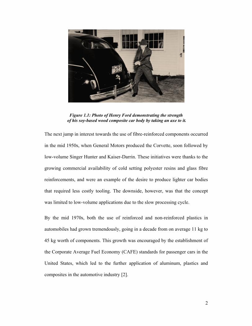
Figure 1.1: Photo of Henry Ford demonstrating the strength of his soy-based
wood composite car body by taking an axe to it. .................................................... 2
Figure 1.2: Photo of Aston Martin V8 Vantage, featuring fibreglass reinforced
composite materials ................................................................................................ 3
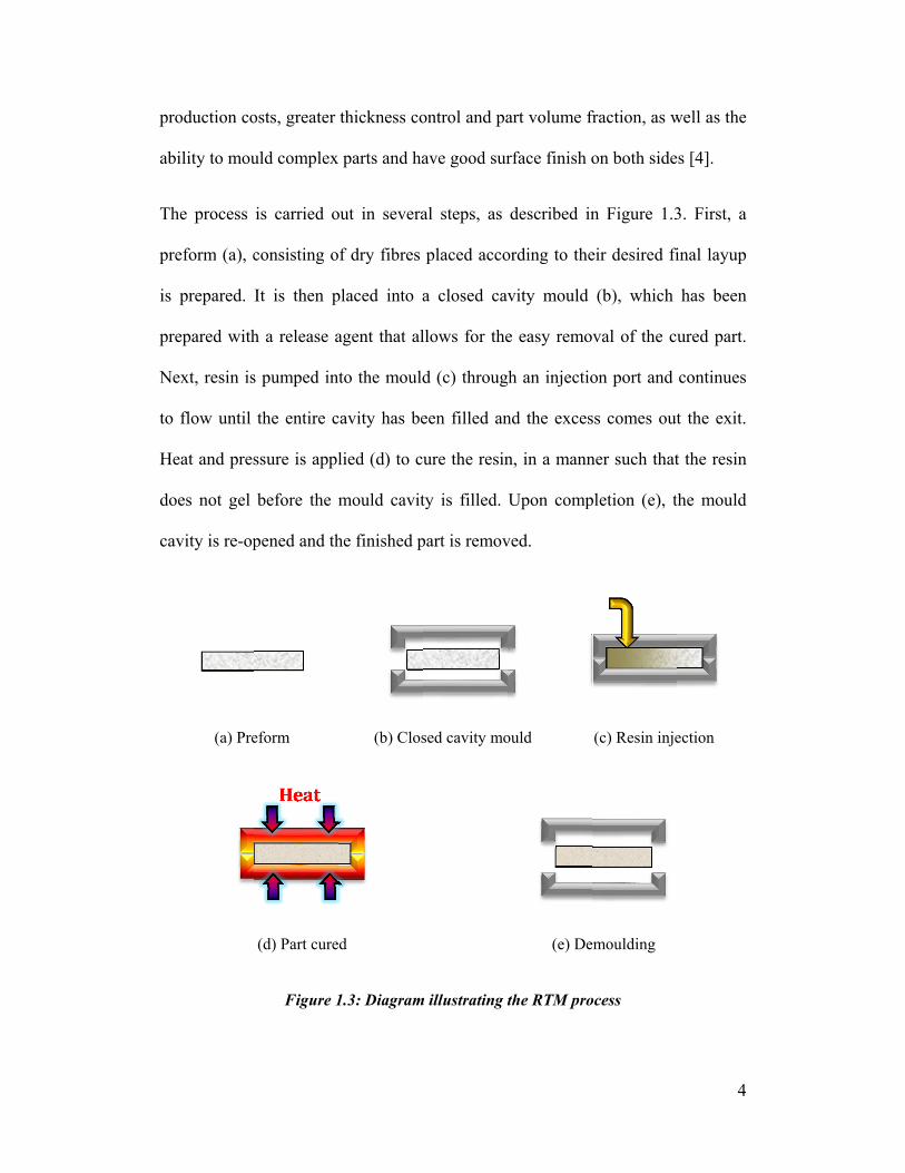
Figure 1.3: Diagram illustrating the RTM process ................................................. 4
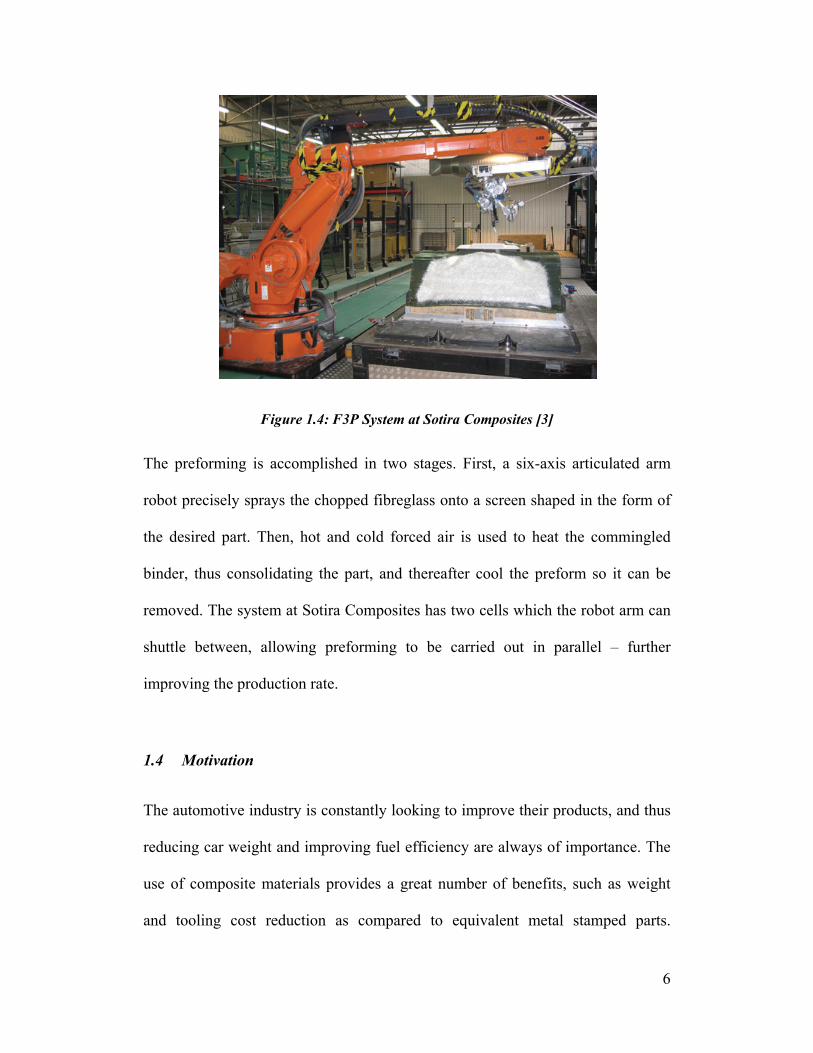
Figure 1.4: F3P System at Sotira Composites [3] ................................................... 6
Figure 2.1: Predicted roughness at filler content of 30 wt% and temperature
gradient of 15°C for a cutoff wavelength of 2.5 mm [11] .................................... 12
Figure 2.2: Selection window for optimum processing parameters at filler content
of 30 wt% and temperature gradient of 15°C, for cutoff wavelengths of 2.5 mm, 8
mm, and 25 mm. The dashed lines indicate the injection time for the preform at
the corresponding injection pressure [12]. ............................................................ 13
Figure 2.3: Comparison between measured resin cure shrinkage and model
prediction under a 90°C isothermal cure condition [13]. ...................................... 15
Figure 2.4: Photos contrasting quantity of scrap material obtained during (a)
conventional thermoforming, (b) F3P robotic preforming of Aston Martin DB9
RH door opening ring [14] .................................................................................... 17
Figure 2.5: Schematic of Ford Programmable Preforming Process (F3P) [16] .... 18
Figure 2.6: Decomposition of surface texture into form, waviness and roughness
[24] ........................................................................................................................ 22
Figure 2.7: Schematic diagram of contact stylus instrument [26] ........................ 24

viii
Figure 2.8: Diagram of ONDULO measurement system [27] .............................. 25
Figure 3.1: Diagram of cross-section of dry F3P fibreglass preform ................... 32
Figure 3.2: Diagram of fixture used to image light transmission through dry
preforms, with sample of acquired image shown in upper-left corner ................. 37
Figure 3.3: Diagram of main steps involved in image analysis using MATLAB
code ....................................................................................................................... 38
Figure 3.4: RTM setup showing the press platens with the preform in the picture
frame ..................................................................................................................... 40
Figure 3.5: Position of temperature (Ti) and pressure (Pi) sensors connected to
DAQ and mounted on RTM press ........................................................................ 42
Figure 3.6: Photograph of ONDULO setup, with composite panel placed between
digital camera and projector screen with phased pattern ...................................... 44
Figure 4.1: Image of preform from Set 2 (Vf = 14%, Top Veil wt% = 15%) with
Class A side facing upwards ................................................................................. 48
Figure 4.2: Image of preform from Set 2 (Vf = 14%, Top Veil wt% = 15%) with
Class A side facing downwards ............................................................................ 49
Figure 4.3: Image of preform from Set 2 (Vf = 14%, Top Veil wt% = 15%) with
background masked out, boundaries and edges indicated, and vertical and
horizontal line profiles drawn. .............................................................................. 50
Figure 4.4: Line profile extracted from light transmission image of dry preform 51
Figure 4.5: Bar chart of average grayscale roughness values for each sample ..... 52
Figure 4.6: Plot of image analysis results – average grayscale roughness values
plotted with respect to fibre volume fraction ........................................................ 53

ix
Figure 4.7: Typical pressure and temperature development during RTM
processing ............................................................................................................. 56
Figure 4.8: Image of test panel 6-1 acquired via the ONDULO system ............... 60
Figure 4.9: Image of ‘best’ region for sample 6-1 obtained from ONDULO system
............................................................................................................................... 61
Figure 4.10: Image of ‘best’ region for sample 6-1 following application of cubic
spline filtering ....................................................................................................... 62
Figure 4.11: Image of ripples in finished part due to flow problems (panel 4-2) 63
Figure 4.12: Image of marks mimicking scratches present on mould surface
(panel 2-1) ............................................................................................................. 63
Figure 4.13: Image of streaks as a consequence of incorrect release agent
application (panel 8-2) .......................................................................................... 64
Figure 4.14: Line profile extracted from filtered ‘best’ region in test panel 2-1 .. 65
Figure 4.15: Roughness motif for line profile of filtered ‘best’ region in test panel
2-1 ......................................................................................................................... 65
Figure 4.16: Bar chart of average roughness values from ONDULO for each
sample ................................................................................................................... 66
Figure 4.17: Plot of ONDULO results – average roughness values plotted with
respect to fibre volume fraction ............................................................................ 67
Figure 8.1: Pressure and temperature development during RTM injection #1 (test
panel 4-1) .............................................................................................................. 81
Figure 8.2: Pressure and temperature development during RTM injection #2 (test
panel 3-1) .............................................................................................................. 82
x
Figure 8.3: Pressure and temperature development during RTM injection #3 (test
panel 6-1) .............................................................................................................. 82
Figure 8.4: Pressure and temperature development during RTM injection #4 (test
panel 7-1) .............................................................................................................. 83
Figure 8.5: Pressure and temperature development during RTM injection #5 (test
panel 2-1) .............................................................................................................. 83
Figure 8.6: Pressure and temperature development during RTM injection #6 (test
panel 1-1) .............................................................................................................. 84
Figure 8.7: Pressure and temperature development during RTM injection #7 (part
scrapped) ............................................................................................................... 84
Figure 8.8: Pressure and temperature development during RTM injection #8 (part
scrapped) ............................................................................................................... 85
Figure 8.9: Pressure and temperature development during RTM injection #9 (test
panel 3-2) .............................................................................................................. 85
Figure 8.10: Pressure and temperature development during RTM injection #10
(test panel 7-2) ...................................................................................................... 86
Figure 8.11: Pressure and temperature development during RTM injection #11
(test panel 1-2) ...................................................................................................... 86
Figure 8.12: Pressure and temperature development during RTM injection #12
(test panel 5-1) ...................................................................................................... 87
Figure 8.13: Pressure and temperature development during RTM injection #13
(test panel 8-1) ...................................................................................................... 87
xi
Figure 8.14: Pressure and temperature development during RTM injection #14
(test panel 4-2) ...................................................................................................... 88
Figure 8.15: Pressure and temperature development during RTM injection #15
(test panel 2-2) ...................................................................................................... 88
Figure 8.16: Pressure and temperature development during RTM injection #16
(test panel 6-2) ...................................................................................................... 89
Figure 8.17: Pressure and temperature development during RTM injection #17
(test panel 8-2) ...................................................................................................... 89
Figure 8.18: Pressure and temperature development during RTM injection #18
(test panel 5-2), note [P4] was unreadable due to a faulty connection ................. 90

xii
List of Tables
Table 3.1: List of resin constituents ...................................................................... 33
Table 3.2: Specific properties of the neat unsaturated polyester resin [5] ............ 33
Table 3.3: Experiment matrix developed by Taguchi method .............................. 36
Table 3.4: List of ONDULO parameters established during testing .................... 45
Table 4.1: Information regarding the RTM processing of each test panel ........... 54
Table 4.2: Quality of surface finish observed in test panels ................................. 58
Table 4.3: ANOVA for image analysis data, based on design factors .................. 68
Table 4.4: ANOVA for ONDULO data, based on design factors ........................ 69
Table 9.1: Average grayscale roughness values for each test panel ..................... 91
Table 9.2: Average grayscale roughness Mean-Squared Deviation results .......... 91
Table 9.3: ONDULO average roughness values for each test panel .................... 92
Table 9.4: ONDULO average roughness Mean-Squared Deviation ..................... 92

xiii
List of Acronyms and Symbols
Acronyms
ACC Automotive Composites Consortium
ANOVA Analysis of Variance
DAQ Data Acquisition System
DOE Design of Experiments
DOI Distinctness-of-Image
DSC Differential Scanning Calorimeter
F3P Ford Programmable Preforming Process
LPA Low Profile Additives
MSD Mean-Squared Deviation
P4 Programmable Powdered Preforming Process
PMMA Polymethyl Methacrylate
PVAc Polyvinyl Acetate
RTM Resin Transfer Moulding
SMC Sheet Moulding Compound
UP Unsaturated Polyester
Symbols
Ga Average Grayscale Roughness
Ra Average Roughness
Vf Fibre volume fraction, measured for cured part
wt% Percent fraction of weight

1
1 Introduction
Improving the surface finish of composite parts manufactured by Resin Transfer
Moulding (RTM) is an important step towards full-scale implementation of such
components in ‘Class A’ automotive applications. Although composite materials
are already being used in the automotive industry, research towards fulfilling the
promise of strong, light weight, high-production parts continues. To place the
current work in context, a glimpse at several past developments in composite
materials for the automotive industry will be presented in Section 1.1. Next, the
RTM process and the Ford Programmable Preforming Process (F3P) will be
introduced in Sections 1.2 and 1.3 respectively. Finally, the motivation and
objectives of this project will be outlined in Sections 1.4 and 1.5.
1.1 A Look at the Past
The use of composites materials is not entirely new to the automotive industry.
Reaching back all the way to the late 1930s, the notion of replacing steel with
more lightweight alternatives existed. It was Henry Ford who made the first
efforts in the field with the introduction of a soy-based wood composite
automobile body, shown in Figure 1.1 [1].
T
in
lo
gr
re
th
w
B
au
4
th
U
co
F of
The next jum
n the mid 19
ow-volume S
rowing com
einforcemen
hat required
was limited to
By the mid
utomobiles h
5 kg worth o
he Corporate
United States
omposites in
Figure 1.1: Pf his soy-base
mp in interest
950s, when G
Singer Hunte
mmercial ava
nts, and were
less costly
o low-volum
1970s, both
had grown tr
of componen
e Average Fu
s, which led
n the automo
Photo of Henred wood comp
towards the
General Mot
er and Kaise
ailability of
e an exampl
tooling. Th
me applicatio
h the use o
remendously
nts. This gro
uel Econom
d to the fur
otive industry
ry Ford demoposite car bod
e use of fibre
tors produce
er-Darrin. Th
cold setting
le of the des
he downside
ons due to th
of reinforced
y, going in a
owth was en
y (CAFE) st
rther applica
y [2].
onstrating thedy by taking a
e-reinforced
ed the Corve
hese initiativ
g polyester r
sire to produ
e, however,
e slow proce
d and non-r
a decade from
ncouraged by
tandards for
ation of alu
e strength an axe to it.
components
ette, soon fol
ves were than
resins and g
uce lighter c
was that the
essing cycle.
reinforced p
m on average
y the establis
passenger c
uminum, pla
2
s occurred
llowed by
nks to the
glass fibre
car bodies
e concept
.
plastics in
e 11 kg to
shment of
cars in the
astics and

3
Currently, the use of composite materials in automotive parts is quite common.
The manufacture of both structural and non-structural components has been
achieved by a number of carmakers, with the processing method of choice being
the Sheet Moulding Compound (SMC) technique. Recently, research seeking to
implement Resin Transfer Moulding (RTM) has gained a great deal of traction.
The application of new fibreglass preforming techniques in conjunction with
RTM has allowed Aston Martin to produce nearly 50 000 composite components
per year for its DB9 Coupe, DB9 Volante (convertible), V8 Vantage (pictured in
Figure 1.2) and V8 Roadster models [3].
Figure 1.2: Photo of Aston Martin V8 Vantage, featuring fibreglass reinforced composite materials
1.2 Resin Transfer Moulding
Resin Transfer Moulding (RTM) is a process whereby dry fibrous reinforcements
are infiltrated with resin and cured in a closed mould. It has garnered a great deal
of attention in the automotive industry thanks to the prospect of reduced
pr
ab
T
pr
is
pr
N
to
H
do
ca
roduction co
bility to mou
The process
reform (a), c
s prepared.
repared with
Next, resin is
o flow until
Heat and pres
oes not gel
avity is re-op
(a) Pre
osts, greater
uld complex
is carried o
consisting o
It is then p
h a release a
s pumped in
the entire c
ssure is appl
before the m
pened and th
eform
(d) Part cure
Figure 1
thickness co
parts and ha
out in severa
f dry fibres
placed into a
agent that al
to the mould
cavity has be
lied (d) to cu
mould cavit
he finished p
(b) Clos
d
1.3: Diagram
ontrol and pa
ave good sur
al steps, as
placed acco
a closed cav
llows for the
d (c) throug
een filled an
ure the resin
ty is filled.
part is remov
sed cavity mo
m illustrating t
art volume fr
rface finish o
described in
ording to the
vity mould
e easy remo
h an injectio
nd the exces
n, in a mann
Upon comp
ved.
ould
(e) De
the RTM pro
fraction, as w
on both side
n Figure 1.3
eir desired fi
(b), which
val of the cu
on port and
ss comes out
ner such that
pletion (e), t
(c) Resin inje
moulding
ocess
4
well as the
s [4].
3. First, a
inal layup
has been
ured part.
continues
t the exit.
t the resin
the mould
ection
5
In the automotive industry, the process is setup such that minimal time is lost
between injection runs. Preforms are prepared outside the mould, and unsaturated
polyester (UP) resins are commonly used because they tend to cost less, cure
more quickly and require lower curing temperatures. The UP resin mixture can
also be manipulated with styrene – to control viscosity, and thermoplastic
particles known as Low Profile Additives (LPA) – to control volumetric shrinkage
during polymerization [5].
1.3 Ford Programmable Preforming Process
The Ford Programmable Preforming Process (F3P) is an automated preforming
technique created by the Ford Motor Co. (Dearborn, MI) in cooperation with
Sotira Composites (Saint Méloir des Ondes, France) and Aston Martin (Gaydon,
Warwick, U.K.). The result of more than a decade of development, the process is
designed to improve preforming efficiency by implementing a robotic system that
reduces scrap and increases production towards high-volume applications [3].
Currently, Aston Martin depends on the combination of F3P and RTM for the
production of nearly 50 000 composite components annually. Displayed in Figure
1.4 is the spraying of chopped fibres onto a component screen.
6
Figure 1.4: F3P System at Sotira Composites [3]
The preforming is accomplished in two stages. First, a six-axis articulated arm
robot precisely sprays the chopped fibreglass onto a screen shaped in the form of
the desired part. Then, hot and cold forced air is used to heat the commingled
binder, thus consolidating the part, and thereafter cool the preform so it can be
removed. The system at Sotira Composites has two cells which the robot arm can
shuttle between, allowing preforming to be carried out in parallel – further
improving the production rate.
1.4 Motivation
The automotive industry is constantly looking to improve their products, and thus
reducing car weight and improving fuel efficiency are always of importance. The
use of composite materials provides a great number of benefits, such as weight
and tooling cost reduction as compared to equivalent metal stamped parts.

7
Additionally, the combination of RTM and F3P allows for improved production
rates, as well as reduced labour needs and scraped material when compared to
other industrial composite processing methods, such as the most commonly used
Sheet Moulding Compound (SMC) [6].
A major concern during the manufacture of composite components by RTM is the
surface finish quality. Parts meant to be placed on the exterior or visible to car
owners are referred to as ‘Class A’ in the automotive industry. Each manufacturer
sets their own metrics for qualifying surface finish, but generally, components
should be free of any noticeable undulations and have an aesthetically pleasing
shine or lustre.
The main factors contributing to the quality of the surface finish of composite
components manufactured by RTM are resin volumetric changes, fibre
characteristics, flow distribution and surface finish of the mould. Work has
previously been carried out to study the optimal resin characteristics and RTM
processing parameters. However, to this point, little is known concerning the
sensitivity of a component’s surface finish to variations in fibre architecture.
Material selection, F3P machine parameters and fibre orientation/distribution are
elements key to fibre preform quality. Thus, in order to obtain a comprehensive
understanding of the material and processing parameters affecting surface finish
in composite components manufactured by RTM, the effect of fibrous
reinforcements must be investigated.
8
1.5 Work objectives and thesis outline
The objective of the current work is to understand the effect varying the
architecture of fibreglass preforms prepared using the Ford Programmable
Preforming Process has on the surface finish quality of composite panels
manufactured by RTM. Parameters determined to be ‘optimal’ in previous work
using the same resin system and moulding apparatus will be maintained. Research
will be accomplished first by identifying the F3P preform characteristics, then by
investigating preform variability, before finally attempting to relate these results
to surface finish.
Chapter 2 will include background information regarding RTM, F3P, the Taguchi
method, surface finish characterisation and preform imaging, as well as insightful
examples of each in literature. The experimental techniques utilised in this project
will be presented in Chapter 3, which will contain details concerning the Taguchi
method, dry preform imaging, RTM processing, and roughness measurements. In
addition to the presentation of results, Chapter 4 will contain discussion regarding
the outcomes, before final conclusions are established in Chapter 5.
9
2 Literature Review
Presented here are the topics deemed to be of relevance to the research work
completed in this thesis. The issues affecting Resin Transfer Moulding, in
particular processing parameters (Section 2.1.1) and resin characterisation
(Section 2.1.2), are discussed in Section 2.1. Fibreglass preform manufacturing is
presented in Section 2.2, with the specific case of the Ford Programmable
Preforming Process in Section 2.2.1. The Taguchi method of design of
experiments is introduced in Section 2.3.1. Section 2.4 includes information
regarding surface finish characterisation, with additional attention being paid to
the ONDULO surface measurement system in Section 2.4.3. A brief exploration
of the concept of preform imaging methods is presented in Section 2.5.
2.1 Resin Transfer Moulding
The increasing demand for less expensive and higher production manufacturing
methods has led the automotive industry towards many new techniques and
materials. In the past, body components were manufactured by metal stamping,
required labour for welding and time for assembly of the many pieces. The
introduction of composites in the automotive industry allowed for a number of
new manufacturing techniques to be implemented. Among them, RTM has gained
a great deal of interest thanks to ability to produce net shape parts, eliminate
finishing operations, allow for greater versatility of reinforcement materials,
reduced waste rate and higher production times [4].
10
There are several factors influencing the overall quality of the finished parts
produced by RTM, ranging from the processing and mould parameters, to the
resin formulation and preform design. Presented in Section 2.1.1 is a review of the
issues affecting RTM processing, while Section 2.1.2 examines the influence of
resin properties.
2.1.1 Processing Parameters
One of the particularities concerning composite materials is that the processes and
tooling required during manufacturing relate directly to the quality of the finished
part. In the case of RTM, the outcome of any part moulding is dependent on the
quality and temperature of the mould faces, location and pressure of the resin
injection and venting.
Previous research aimed to understand the effect each of these parameters has on
the moulding process. Karbhari et al. [7] studied the effect of material, process
and equipment variables on tension, shear and bending of composite parts using
the Taguchi design of experiments method. It was determined that stroke length,
an injection piston parameter, had the most influence on the performance of RTM
parts. The experiments revealed that depending on the design space studied, some
factors appeared to be insensitive to change. Surface finish and filling time were
used as response metrics by Dutiro [8] to research the factors affecting RTM
processing. Injection pressure, filler content, glass fibre volume fraction and
mould temperature were examined using a quadratic design technique. Improved
surface finish was seen in cases where injection pressure was increased and fibre

11
volume fraction decreased, though resin filler content was the most influential
factor. Meanwhile, gloss increased with reduced filler content and lower mould
temperatures [9]. Bayldon [10] concluded that higher filler content and injection
pressure improve roughness and gloss measures, though limiting benefits were
observed as the filler caused difficulties in filling the mould cavity.
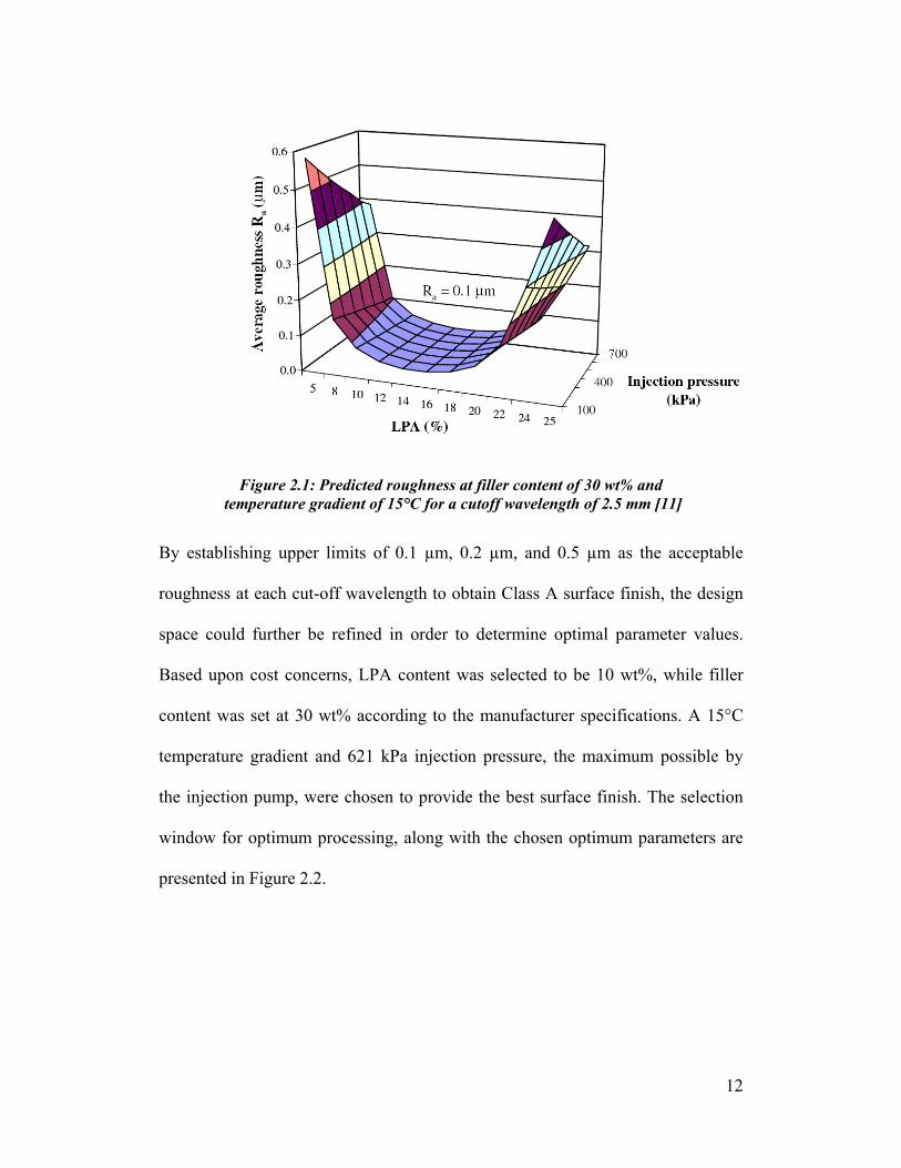
Work was carried out by Raja [5], seeking to determine optimal process
parameters for Class A surface finish in RTM. A surface roughness prediction
model was developed to include the effect of LPA content, filler content,
temperature gradient between moulds and injection pressure. Test composite
panels were manufactured using a fibreglass preform and unsaturated polyester
resin system according to an experiment matrix designed based on the Taguchi
method. Surface roughness results obtained from a contact profilometer with filter
cut-off wavelengths of 2.5 mm, 8 mm and 25 mm were used to establish the value
of each fitting constant based on non-linear regression analysis, therefore
providing a goodness of fit calculated to be R2 = 0.96. The general form of the
model representing the average roughness, Ra (μm), is given by:
)( 654322
10 CFFECAAa eR βββββββ ++++++= Eq. 2.1
where βi (i = 0-6) are fitting constants, A is LPA content (wt%), C is filler content
(wt%), E is temperature gradient (°C) and F is injection pressure (kPa) [11].
Figure 2.1 displays the 3-D parabola obtained when filler content and temperature
gradient are fixed.
12
Figure 2.1: Predicted roughness at filler content of 30 wt% and temperature gradient of 15°C for a cutoff wavelength of 2.5 mm [11]
By establishing upper limits of 0.1 µm, 0.2 µm, and 0.5 µm as the acceptable
roughness at each cut-off wavelength to obtain Class A surface finish, the design
space could further be refined in order to determine optimal parameter values.
Based upon cost concerns, LPA content was selected to be 10 wt%, while filler
content was set at 30 wt% according to the manufacturer specifications. A 15°C
temperature gradient and 621 kPa injection pressure, the maximum possible by
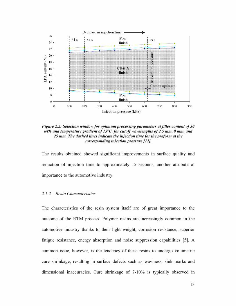
the injection pump, were chosen to provide the best surface finish. The selection
window for optimum processing, along with the chosen optimum parameters are
presented in Figure 2.2.
13
Figure 2.2: Selection window for optimum processing parameters at filler content of 30 wt% and temperature gradient of 15°C, for cutoff wavelengths of 2.5 mm, 8 mm, and
25 mm. The dashed lines indicate the injection time for the preform at the corresponding injection pressure [12].
The results obtained showed significant improvements in surface quality and
reduction of injection time to approximately 15 seconds, another attribute of
importance to the automotive industry.
2.1.2 Resin Characteristics
The characteristics of the resin system itself are of great importance to the
outcome of the RTM process. Polymer resins are increasingly common in the
automotive industry thanks to their light weight, corrosion resistance, superior
fatigue resistance, energy absorption and noise suppression capabilities [5]. A
common issue, however, is the tendency of these resins to undergo volumetric
cure shrinkage, resulting in surface defects such as waviness, sink marks and
dimensional inaccuracies. Cure shrinkage of 7-10% is typically observed in
14
unsaturated polyester (UP) resins, thus complicating the task of achieving Class A
finish in composite parts [2].
The use of techniques allowing for the thermal, rheological and morphological
characterization, have allowed for a better understanding of the resin system.
Research on the topic has focused on compensating for the volumetric cure
shrinkage by the introduction of thermoplastic particles, called Low Profile
Additives (LPA). Although the underlying principles of LPAs are not well
understood, much work has been completed seeking to understand their
behaviour. Thermal expansion during high temperature cure, phase separation
between LPA and UP resin, and micro-void formation at the LPA/UP interface
are generally accepted to be the mechanisms behind the expansion of the resin
system.
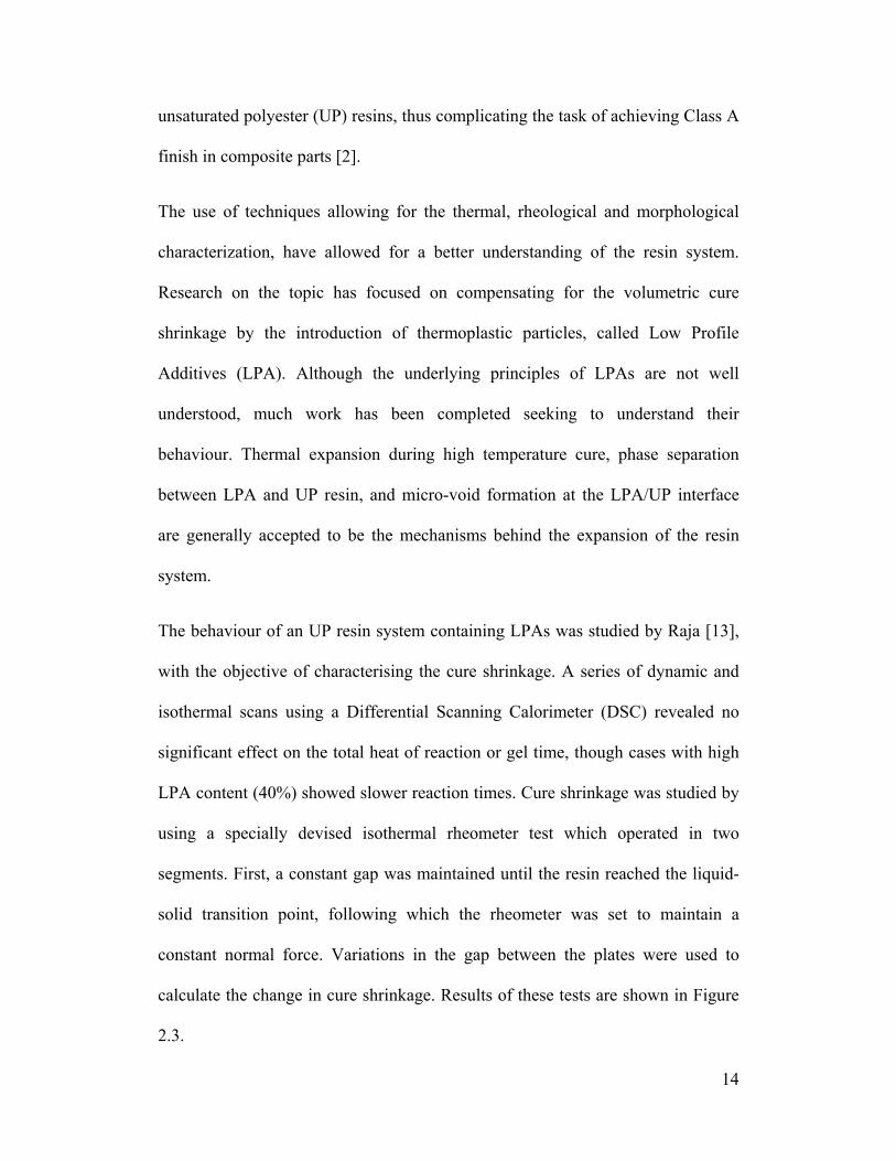
The behaviour of an UP resin system containing LPAs was studied by Raja [13],
with the objective of characterising the cure shrinkage. A series of dynamic and
isothermal scans using a Differential Scanning Calorimeter (DSC) revealed no
significant effect on the total heat of reaction or gel time, though cases with high
LPA content (40%) showed slower reaction times. Cure shrinkage was studied by
using a specially devised isothermal rheometer test which operated in two
segments. First, a constant gap was maintained until the resin reached the liquid-
solid transition point, following which the rheometer was set to maintain a
constant normal force. Variations in the gap between the plates were used to
calculate the change in cure shrinkage. Results of these tests are shown in Figure
2.3.
15
Figure 2.3: Comparison between measured resin cure shrinkage and model prediction under a 90°C isothermal cure condition [13].
Cure shrinkage is compensated for in cases where LPA content ranges from 10-
20%, while content of 40% and below 10% still show cure shrinkage in the cured
resin. A resin LPA content of 10% was selected as ideal based on phase
separation, micro-void formation and minimum cost.
2.2 Fibreglass Preform Manufacturing
Another key factor contributing to the overall quality of composite components is
the reinforcement material. In order to replace metal structural, semi-structural
and Class A parts, the automotive industry has turned to composites made with
reinforcements ranging from carbon and glass, all the way to natural fibres [1].
The great necessity for such applications, however, is the ability to produce high
16
volumes of strong parts at a high rate and low cost. For Class A components, the
standard has been the use of glass fibres, with the Sheet Moulding Compound
(SMC) process being most popular [14]. The potential benefits of RTM
processing, however, have created a need for high-rate fibreglass preforming, and
thus research in the field has grown.
The first step towards the application of high-volume preforming was in 1988
with the creation of the Automotive Composites Consortium (ACC), a research
effort fashioned by Ford, General Motors and Chrysler, and sponsored by the U.S.
Department of Energy. The program was seeking to carry out pre-competitive
research in the area of polymer composites for structural applications. The result
was a technique called the Programmable Powdered Preforming Process (P4)
which carried out automated deposition of chopped glass fibres. By having
screens shaped like the part and with a partial vacuum applied, fibres could be
held in place until a powdered binder was sprayed into place and the preform
compacted and heated to be consolidated and moved to the resin infusion mould
[15].
2.2.1 Ford Programmable Preforming Process
Based upon the expertise gained from the P4 technique, Ford Research and Aston
Martin developed the Ford Programmable Preforming Process (F3P) system in
cooperation with Sotira Composites. This system, refined by researchers for
industrial production, fulfilled the need for fibreglass preforming towards the
manufacture of several Aston Martin models, such as the V12 Vanquish
17
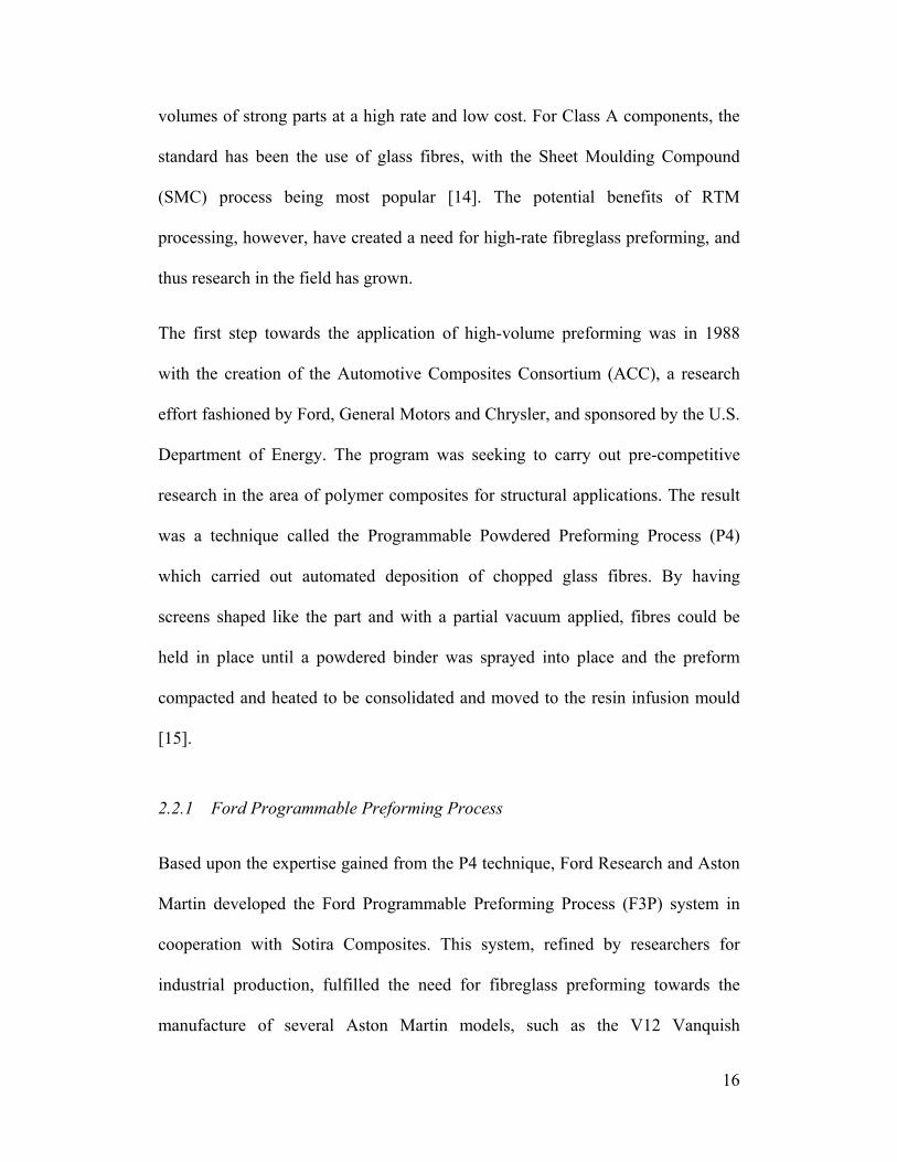
introduced in 2001, which incorporated 26 composite components [3]. Shown in
Figure 2.4 are images contrasting the quantity of scrap produced in (a)
conventional thermoforming processes, and (b) F3P robotic preforming. Other
benefits resulting from the new design technique include the ability to change
mould tools quickly (~10 minutes), the flexibility to vary fibre length and areal
density accurately, and the capability of manufacturing multiple components for a
variety of car models.
(a) Conventional Thermoforming (b) F3P Robotic Preforming
Figure 2.4: Photos contrasting quantity of scrap material obtained during (a) conventional thermoforming, (b) F3P robotic preforming of
Aston Martin DB9 RH door opening ring [14]
Developmental work on the F3P system over the past decade have led operators to
the selection and use of 3469 tex PREFORMance glass rovings manufactured by
PPG Industries Inc., which commingles a thermoplastic polymer ‘string’ binder
directly into the rovings [3]. A fine 1200 tex low-density veil roving supplied by
Owens Corning Composite Solutions LLC without any binder is used on surfaces
requiring good surface finish. These changes were made to the original system in
order to prevent machine clogging that occurred due to the use of powdered
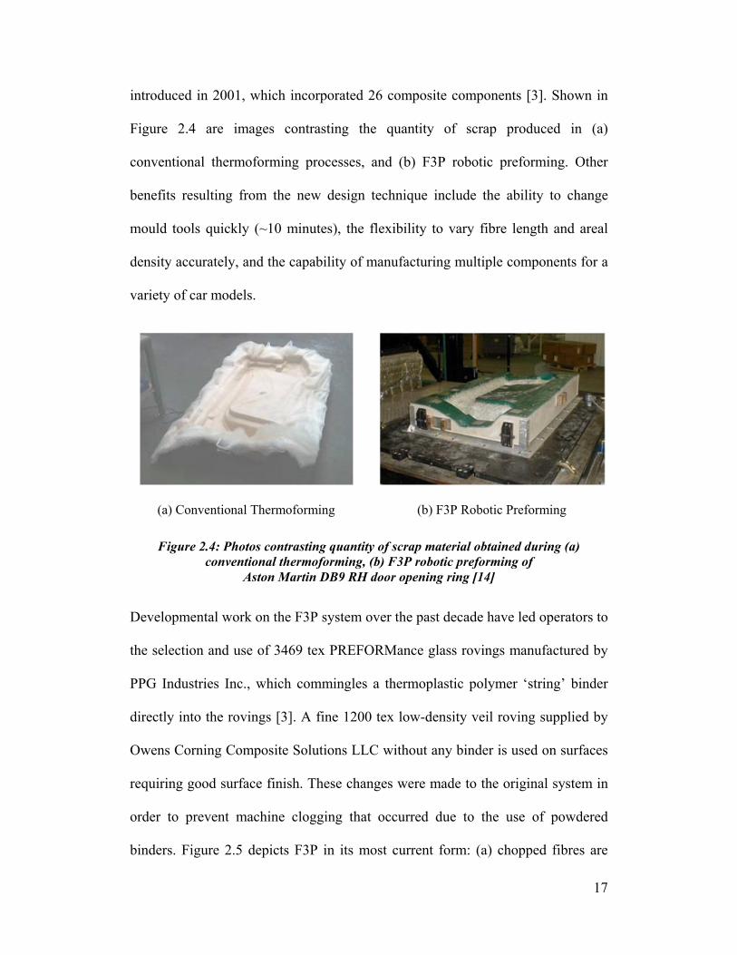
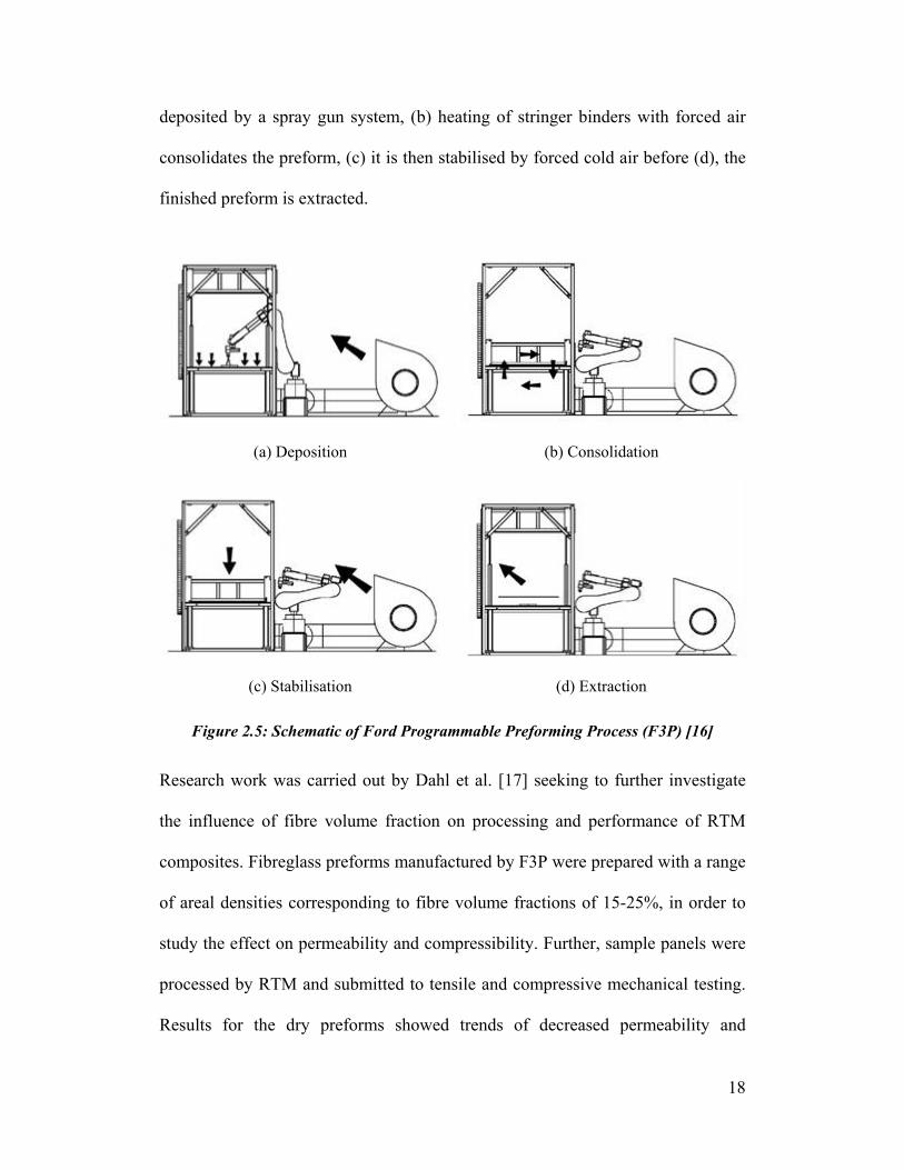
binders. Figure 2.5 depicts F3P in its most current form: (a) chopped fibres are
18
deposited by a spray gun system, (b) heating of stringer binders with forced air
consolidates the preform, (c) it is then stabilised by forced cold air before (d), the
finished preform is extracted.
(a) Deposition (b) Consolidation
(c) Stabilisation (d) Extraction
Figure 2.5: Schematic of Ford Programmable Preforming Process (F3P) [16]
Research work was carried out by Dahl et al. [17] seeking to further investigate
the influence of fibre volume fraction on processing and performance of RTM
composites. Fibreglass preforms manufactured by F3P were prepared with a range
of areal densities corresponding to fibre volume fractions of 15-25%, in order to
study the effect on permeability and compressibility. Further, sample panels were
processed by RTM and submitted to tensile and compressive mechanical testing.
Results for the dry preforms showed trends of decreased permeability and
19
increased compaction pressure as the fibre volume fraction increased. Mechanical
testing revealed trends of increasing tensile modulus, strength and strain-to-failure
for increased fibre volume fraction – while no influence was seen in compressive
strength. Moreover, an observed decrease in permeability existed due to the
introduction of surface veils.
Probabilistic and sensitivity analysis was carried out by Bebamzadeh et al. [18],
allowing for the calculation of relative importance of a number of processing
parameters. Finite element reliability analysis was used to obtain rankings
showing distance between fibres, fibre diameter, and volumetric resin cure
shrinkage as the most important factors contributing to maximum surface
waviness of 0.25 µm.
Based upon input from Aston Martin [19], it is known that the inherent quality of
a preform is defined by three factors: fibre selection, machine parameters, and
fibre distribution. The selection of the manufacturer and the type of glass fibres
and binder systems to be used constitute the fibre selection. Machine parameters
include: design of the chopper gun, spray rate, spray pattern, and fibre ejection
parameters. As discussed, developmental work has previously been carried out to
determine proprietary fibre selection and machine parameters. The variations in
fibre distribution are fibre areal density and surface veil thickness. Currently, the
sensitivity of Class A surface finish to variations in fibre distribution is not well
understood and requires further study.

20
2.3 Design of Experiments
Experimentation is an important step in the development of any process or the
understanding of any concept. Design of Experiments (DOE) is a scientific
approach allowing for the study of the relationship between experimental inputs
and the resulting outputs. In its most basic of forms, DOE represents the use of
statistical analysis to study the effects of multiple factors at once, as opposed to
the tedious study of a single experimental parameter at a time. The technique was
first introduced by Sir Ronald A. Fisher in England in the early 1920s, with the
goal of determining optimum water, rain, sunshine, fertilizer, and soil conditions
needed to produce the best crop [20]. Classical DOE consisted of varying factors
in order to graph trends in performance and determine the optimal performance
for each variable. Much research and development in the field followed, but the
applications of classical DOE remained limited to academic environments.
2.3.1 Taguchi Method
Enter Dr. Genichi Taguchi, who developed a new technique with the idea in mind
that quality is measured by consistency of performance. Referred to as the
Taguchi method, this technique seeks to reduce the distance between the mean
and the target value, as well as minimise the standard deviation in the results
obtained for a given test population [21]. This is accomplished thanks to the use
of a set of tables, known as orthogonal arrays, which enable the main variables in
a given experiment to be investigated in a minimal number of trials.

21
The Taguchi method is prepared for a given application in several steps. First, the
objectives of the project are determined, with specific quality characteristics and
evaluation metrics established. This is carried out by researchers with knowledge
of the given design space and experiment scope. Next, a broad set of factors
thought to influence the results are considered, and the number of trials to be
completed is selected. The suspected behaviour of each variable, along with the
number of degrees-of-freedom which the orthogonal array can accommodate, is
used to establish the number of levels to be studied. Finally, the key factors which
suit the experiment plan are chosen based upon the size of the design array. The
result of this preparation is a test matrix consisting of the most significant factors
studied at specific variable levels.
The next step in the Taguchi method is the carrying out of the experimental trials
as planned, thus generating results based on the evaluation of the samples which
allow for statistical calculations to be completed. The formulas and procedures
used for the Taguchi method are referred to as Analysis of Variance (ANOVA). It
accounts for variability over multiple trials by calculating how much the variation
in each factor contributes to the total variations observed in the results. Further,
within this analysis, the consistency of performance is measured by what is called
the Mean-Squared Deviation (MSD), which allows for the study of all sorts of
data. Depending on the desired criteria, either the minimum MSD or trends within
each factor can be used to determine optimal parameters for a given experiment,
as well as the corresponding estimated performance.
22
2.4 Surface Finish Characterisation
The surface of an object can be defined as the boundary that separates it from the
surrounding medium, as per the ANSI/ASME standard [22]. This is a very broad
description of the concept, but it provides a good basis for characterisation to be
carried out. One can imagine that if a material was cut and the cross-section were
analysed, it would be the 2-D profile produced by the boundary of this object that
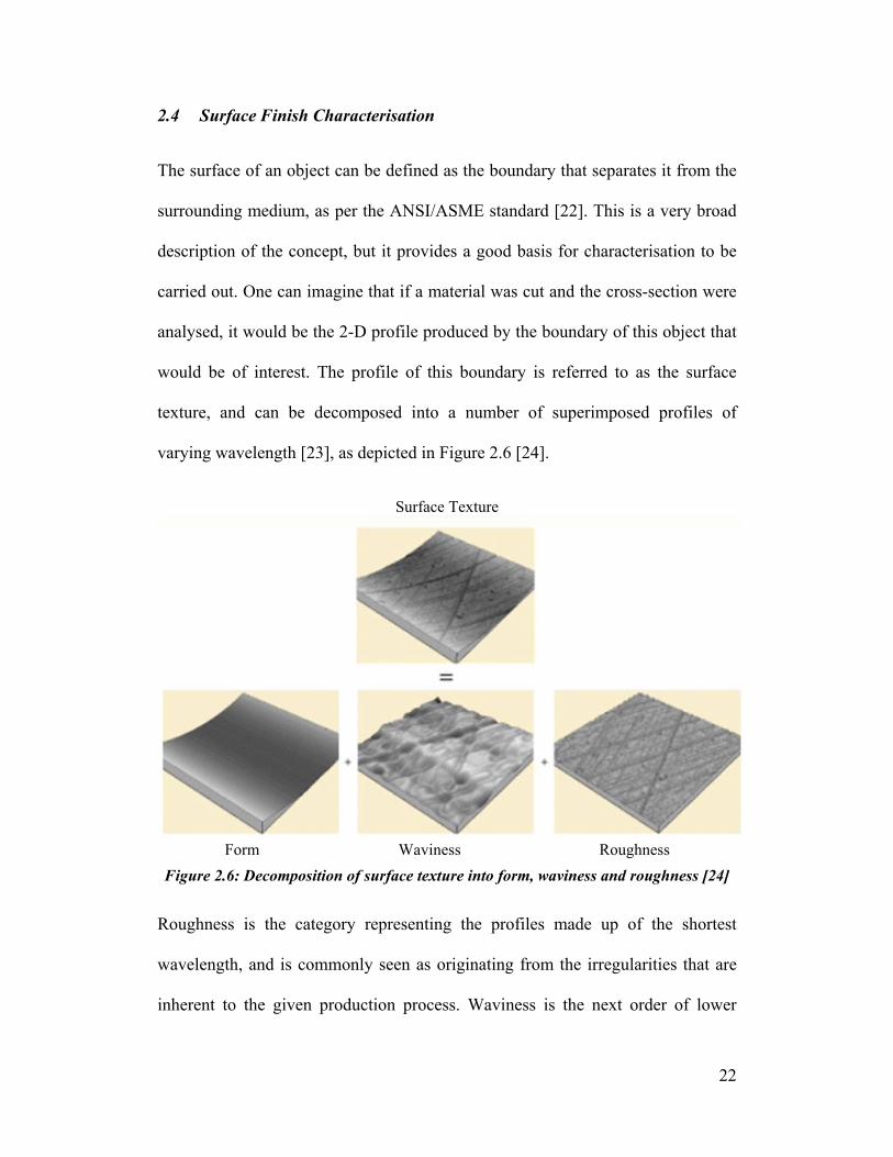
would be of interest. The profile of this boundary is referred to as the surface
texture, and can be decomposed into a number of superimposed profiles of
varying wavelength [23], as depicted in Figure 2.6 [24].
Surface Texture
Form Waviness Roughness Figure 2.6: Decomposition of surface texture into form, waviness and roughness [24]
Roughness is the category representing the profiles made up of the shortest
wavelength, and is commonly seen as originating from the irregularities that are
inherent to the given production process. Waviness is the next order of lower

23
frequency and comes from a variety of causes. Finally, form is the longest
wavelengths, and represents the deviations from the nominal surface shape.
2.4.1 Class A Surface Finish
‘Class A’ is a term used to describe the finish deemed to be acceptable for exterior
parts in the automotive industry. Dutiro describes Class A finish as exhibiting
“aspects of flatness, smoothness, and light reflection similar to that of finished
stamped steel sheeting, typically with a DOI (Distinctness-of-image) values
between 60-90, as measured with D-Sight optical enhancement techniques” [9].
There is no one standard, but components should be aesthetically pleasing,
smooth and without noticeable defects – thus mimicking an equivalent metal
component which is perfectly polished, free of porosity or scratches, and with a
high lustre finish. In industry, composite components are polished, primed, and
then finished with paint which is sprayed over allowing for inconsistencies to be
filled. The cost and labour required for this work, however, can be reduced by
improving processing methods and moulding techniques. The use of resin
formulations that appropriately compensate for expansion/shrinkage mechanisms,
as well as appropriate tool and processing parameter design allows for superior
part quality.
2.4.2 Surface Texture Measurements
The techniques used in order to map the profile of a given surface can be
categorized as contact or non-contact methods. Contact methods scan the
24
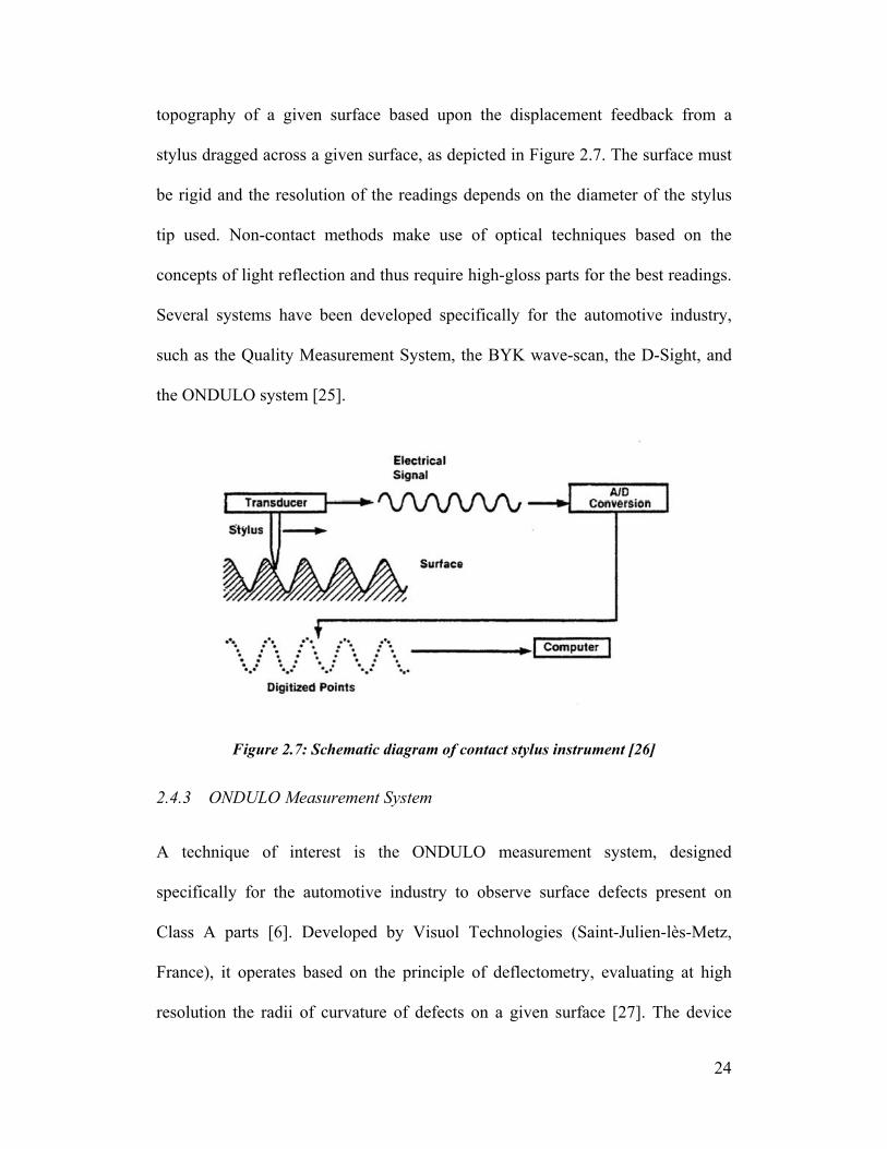
topography of a given surface based upon the displacement feedback from a
stylus dragged across a given surface, as depicted in Figure 2.7. The surface must
be rigid and the resolution of the readings depends on the diameter of the stylus
tip used. Non-contact methods make use of optical techniques based on the
concepts of light reflection and thus require high-gloss parts for the best readings.
Several systems have been developed specifically for the automotive industry,
such as the Quality Measurement System, the BYK wave-scan, the D-Sight, and
the ONDULO system [25].
Figure 2.7: Schematic diagram of contact stylus instrument [26]
2.4.3 ONDULO Measurement System
A technique of interest is the ONDULO measurement system, designed
specifically for the automotive industry to observe surface defects present on
Class A parts [6]. Developed by Visuol Technologies (Saint-Julien-lès-Metz,
France), it operates based on the principle of deflectometry, evaluating at high
resolution the radii of curvature of defects on a given surface [27]. The device
25
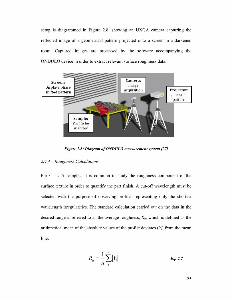
setup is diagrammed in Figure 2.8, showing an UXGA camera capturing the
reflected image of a geometrical pattern projected onto a screen in a darkened
room. Captured images are processed by the software accompanying the
ONDULO device in order to extract relevant surface roughness data.
Figure 2.8: Diagram of ONDULO measurement system [27]
2.4.4 Roughness Calculations
For Class A samples, it is common to study the roughness component of the
surface texture in order to quantify the part finish. A cut-off wavelength must be
selected with the purpose of observing profiles representing only the shortest
wavelength irregularities. The standard calculation carried out on the data in the
desired range is referred to as the average roughness, Ra, which is defined as the
arithmetical mean of the absolute values of the profile deviates (Yi) from the mean
line:
∑=n
iia Y
nR 1
Eq. 2.2
26
Work carried out by DeBolt [28] studied the effectiveness of several measurement
techniques and roughness calculation wavelength cut-offs. Band pass filtering was
carried out on the profiles obtained, after which the surface finish was quantified
within certain frequency ranges. It was determined that selection of appropriate
cut-off wavelengths was of critical importance to understanding the quality of a
Class A surface. Palardy [12] utilised both a contact profilometer, and the
contactless ONDULO system to study the effect of painting processes on the
surface finish of RTM panels. For the evaluation of Ra, a cut-off wavelength of
2.5 mm was used, as per ISO 4288:1996 [29]. This allowed for differences in
finish quality to be measured and compared, thus permitting the establishment of
optimal process parameters. Schubel et al. [30] studied the surface quality of
coated and uncoated composite panels. It was determined that the mean roughness
parameter is suitable for relating bare laminates to final painted quality, and that
light reflectometry correlates well with subjective assessments for painted
laminates.
2.5 Preform Imaging Methods
Little work has been carried out in the literature studying the use of digital
imaging to qualify fibreglass preforms prior to RTM manufacturing. This is a
technique conceived so as to obtain relevant information regarding attributes such
as variations in local areal density, top surface patterns, and presence of defects.
The gathered information can be used to validate the adequacy of a preform, or
predict the finished outcome following resin injection moulding. The work carried
27
out in this project on the topic of preform imaging is a novel adaptation of this
concept.
Recently, a study that parallels the work in this project has been carried out by
Gan et al. [31] at the University of Auckland. This work, as yet unpublished,
studies the variability of reinforcement material using a ‘lightbox’ upon which
samples could be placed and photographed by a mounted digital camera. By
calculating the discrepancy between a platform with and without a preform
present, a gray level value representing the light blocked by the preform is
calculated. Analysis of pixel values allows for the determination of localised areal
density calculations, and thereafter the ability to proceed with statistical preform
characterisation.
2.6 Summary of Literature Review
The purpose of this chapter has been to present the literature reviewed during the
course of the research carried out for this project. A great deal of information was
gathered concerning the optimization of processing Class A composites by RTM.
The most influential factors contributing to good surface finish are injection
pressure, control of volumetric cure shrinkage/expansion, mould surface quality,
and resin filler content. Further, an understanding of the use of Low Profile
Additives (LPA) to compensate for volumetric changes was gained.
An investigation into the Ford Programmable Preforming Process (F3P) revealed
the importance of machine, material and architecture parameters. Much

28
developmental work has already been completed in industry, though further study
is required regarding the effect of fibre distribution on surface finish.
The Taguchi method of design of experiments is preferred for design of
experiments, having successfully led previous researchers to the determination of
optimal experiment parameters, in addition to understanding of the process
studied.
Characterisation of surface finish has previously been accomplished by through
the use of average roughness (Ra) values, calculated from line profiles extracted
from surface topography. This data has successfully been obtained from both
contact (stylus) and non-contact (optical) methods. The ONDULO system, a non-
contact method, is a technique of interest, thanks to its design specifically for the
purpose of imaging Class A surfaces in the automotive industry.
2.7 Research Objectives
The current work is one of the final pieces of the puzzle in a collaborative effort
with research groups from the École Polytechnique de Montréal and the
University of British Columbia. As part of the Auto21 Network of Centres of
Excellence, this project, entitled “Optimization of Composite Manufacturing by
Resin Injection”, aims to help fulfill the promise of RTM manufacturing in the
automotive industry. The role of McGill University in this project is to
characterise the resin and preform materials through the use of RTM experiments,
focusing mainly on the sensitivity of Class A surface finish to these parameters.

29
This thesis builds upon the resin characterisation and process optimization carried
out by Mohsan H. Raja’s PhD thesis [5] and Geneviève Palardy’s Master’s thesis
[2]. Their research investigated the manufacture of composite parts by RTM
according to six parameters: LPA (wt%), styrene (wt%), filler (wt%), gel time
(min), temperature gradient between moulds (°C) and injection pressure (kPa). A
total of 18 fibreglass/UP test panels were moulded and evaluated as per the
Taguchi method. A contact profilometer was used to quantify surface roughness,
and results were studied by ANOVA, following which a set of optimal parameters
were established. Validation test samples were manufactured, and resin
volumetric changes were studied using cure kinetics and rheometry methods.
Further, the sensitivity of the surface finish to typical painting processes was
studied, and ideal heating cycles were suggested.
The objective of the current work is to study the effect of preform variability on
the surface finish of Class A composite parts manufactured by RTM. The main
goals to be accomplished are:
1. Determine preform characteristics: Preform attributes of interest to surface
finish will be selected and a test matrix suitable for investigating
variability will be established.
2. Determine quality of dry preforms: A method by which preforms can be
qualified prior to injection moulding will be established.
3. Surface finish characterisation: Test composite panels will be
manufactured, after which surface roughness will be evaluated.

30
4. Relate results to surface finish: The variations in preform quality prior to
and following moulding will be related.

31
3 Experimental Procedures
Presented is an outline of the experimental procedures used to study how the
variability of fibreglass preforms effects surface finish in Class A composite parts.
Section 3.1 describes the materials used throughout the experimental portion of
this project. Section 3.2 contains the details regarding the formation of an
appropriate experimental test matrix. Next, a novel preform imaging technique
used in this thesis is explained in Section 3.3. The RTM process employed for the
manufacture of composite test panels is detailed in Section 3.4. Finally, the
procedure applied to obtain measurements characterising the surface finish of test
panels is detailed in Section 3.5.
3.1 Materials
The set of materials used for experimentation consisted of fibreglass preforms
produced by the F3P technique, and an unsaturated polyester (UP) resin obtained
from Scott Bader Company Ltd.
3.1.1 Fibreglass Preforms
Preforms were obtained from Sotira Composites according to specifications as
determined by the orthogonal array established via Taguchi design of experiments
(Section 3.2). Individual samples were cut to 26 cm x 24cm from the 80 cm x 120
cm sheets received. The architecture of the preforms consisted of structural fibres
symmetrically sandwiched between layers of surface veil fibres, as seen in Figure

32
3.1. On the side meant to be for Class A finish, the veil fibres were sprayed down
in a criss-crossing manner, thus creating a lattice pattern.
Figure 3.1: Diagram of cross-section of dry F3P fibreglass preform
Developmental work on the F3P system over the past decade has led operators to
the selection and use of 3469 tex PREFORMance glass rovings, which
commingles a thermoplastic polymer ‘string’ binder directly into the roving. A
fine 1200 tex low-density veil roving without any binder was used on surfaces
requiring good surface finish. Details regarding the glass fibres used in the F3P
method are listed below:
• Structural Fibres: PPG Industries Inc. – PREFORMance
o 3469 tex rovings
o 25.4 mm fibre length
o Contains up to 6-7 wt% string binder
• Veil Fibres: Owens Corning Composite Solutions LLC
o 1200 tex low-density veil rovings
o No binder present
33
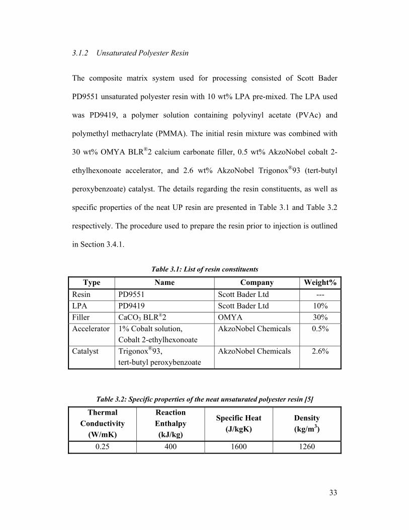
3.1.2 Unsaturated Polyester Resin
The composite matrix system used for processing consisted of Scott Bader
PD9551 unsaturated polyester resin with 10 wt% LPA pre-mixed. The LPA used
was PD9419, a polymer solution containing polyvinyl acetate (PVAc) and
polymethyl methacrylate (PMMA). The initial resin mixture was combined with
30 wt% OMYA BLR®2 calcium carbonate filler, 0.5 wt% AkzoNobel cobalt 2-
ethylhexonoate accelerator, and 2.6 wt% AkzoNobel Trigonox®93 (tert-butyl
peroxybenzoate) catalyst. The details regarding the resin constituents, as well as
specific properties of the neat UP resin are presented in Table 3.1 and Table 3.2
respectively. The procedure used to prepare the resin prior to injection is outlined
in Section 3.4.1.
Table 3.1: List of resin constituents
Type Name Company Weight%Resin PD9551 Scott Bader Ltd --- LPA PD9419 Scott Bader Ltd 10% Filler CaCO3 BLR®2 OMYA 30% Accelerator 1% Cobalt solution,
Cobalt 2-ethylhexonoate AkzoNobel Chemicals 0.5%
Catalyst Trigonox®93, tert-butyl peroxybenzoate
AkzoNobel Chemicals 2.6%
Table 3.2: Specific properties of the neat unsaturated polyester resin [5]
Thermal Conductivity
(W/mK)
Reaction Enthalpy (kJ/kg)
Specific Heat (J/kgK)
Density (kg/m3)
0.25 400 1600 1260

34
3.2 Design of Experiments
The first step towards understanding the contribution of F3P fibreglass preforms
to the surface finish of Class A parts is characterising the preforms themselves.
Thus, the factors which are known to contribute to the quality of a preform must
be understood such that variability may be studied. Based upon input from Aston
Martin, it was concluded that the inherent quality of a preform was defined by
three factors: fibre selection, machine parameters, and fibre distribution. As
previously discussed, much developmental work has been carried out in order to
select the appropriate materials for F3P. Additionally, although the actual
machine parameters would be of interest to study, an intimate knowledge and
direct access to the system would be required – this was not possible due to the
fact that the F3P setup is already involved in manufacturing on the order of 50
000 units per year.
3.2.1 Taguchi Method
Thus, it was decided that the focus of the project would be to study how fibre
distribution affects surface finish. For the purposes of this research, the Taguchi
technique for design of experiments was implemented. Planning a set of
experiments according to this technique required first the selection of primary
objectives and metrics by which results could be measured and compared. For this
project, the goal was to study the contribution of fibre reinforcement parameters
using mean roughness values calculated from measured surface profiles. Next,
starting from a wide range of contributors, the most important factors were

35
selected. Having dismissed fibre selection and machine parameters, the focus was
set on fibre distribution – within which the two major factors easily varied and of
importance to surface finish are the preform areal density and the weight fraction
of the surface veil. Taking into consideration the known acceptable range and the
potential number of trials required, it was decided that the factors would be
studied on 4- and 2-levels respectively.
Previously, for work carried out by Raja [5], the F3P system was programmed to
output a glass fibre areal density of 1626 g/m2, which corresponds to a fibre
volume fraction (Vf) of 20% for parts with a thickness of 3.175 mm. The structural
fibres totalled 81.8% of the total weight fraction of the preforms, with each of the
top and bottom veil fibres equalling 9.1% by weight of the preform.
As the final step towards the formulation of a test matrix, the specific levels of
each factor were selected. Assuming that surface finish could be improved by
increasing the resin content and thickening the surface veil, factor levels exploring
the range of surrounding the 20% volume fraction and 9.1% veil weight fraction
were decided upon. Having determined that the experiment would consist of one
4-level and one 2-level factor, the Taguchi technique dictated that the minimum
number of trials needed would be 8, thus making use of an upgraded L-8 array, as
presented in Table 3.3. It is important to note that values of fibre volume fraction
are calculated based on the moulded part thickness of 3.175 mm, thus values of
14%, 17%, 20%, and 23% corresponded to fibre areal densities of 1138, 1382,
1626, and 1870 g/m2 for dry preforms. Also, the top veil wt% and bottom veil

36
wt% will always be identical since the F3P preforms obtained were designed to be
symmetric apart from the existence of the top veil lattice pattern.
Table 3.3: Experiment matrix developed by Taguchi method
Set Preform Vf (%) Top Veil wt% 1 14 10 2 14 15 3 17 10 4 17 15 5 20 10 6 20 15 7 23 10 8 23 15
3.3 Preform Imaging Technique
Since local variations in the quality of fibreglass reinforcements are not obvious
following injection moulding, it is of interest to obtain images detailing the fibre
distribution of preforms in their dry state prior to moulding. The hope of this
exercise is to gain further information regarding the relative quality of preforms
and how it relates to moulded parts. A novel technique whereby fibrous
reinforcements were photographed with the goal of emphasizing local changes in
areal density was implemented in this project.
3.3.1 Light Transmission Fixture
The test setup consisted of a fluorescent light source enclosed in a box and capped
by a 3.175 mm white acrylic sheet serving as a light diffuser. Dry fibrous
reinforcements were placed onto the acrylic sheet and photographed such that a
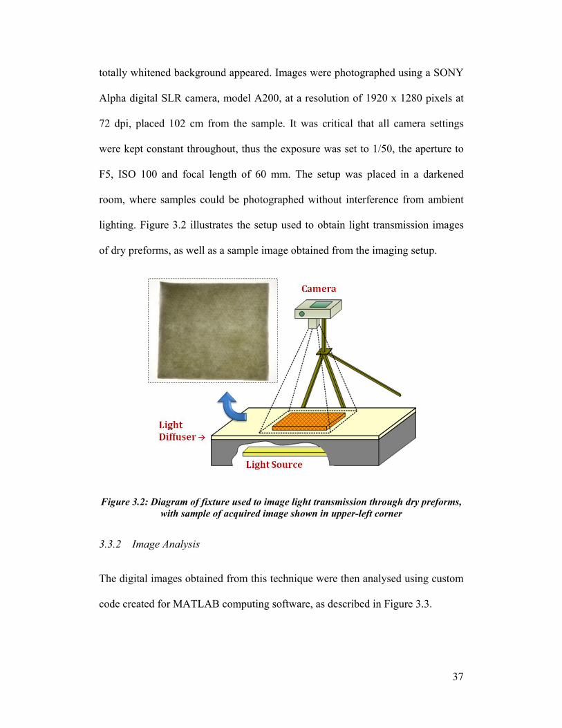
37
totally whitened background appeared. Images were photographed using a SONY
Alpha digital SLR camera, model A200, at a resolution of 1920 x 1280 pixels at
72 dpi, placed 102 cm from the sample. It was critical that all camera settings
were kept constant throughout, thus the exposure was set to 1/50, the aperture to
F5, ISO 100 and focal length of 60 mm. The setup was placed in a darkened
room, where samples could be photographed without interference from ambient
lighting. Figure 3.2 illustrates the setup used to obtain light transmission images
of dry preforms, as well as a sample image obtained from the imaging setup.
Figure 3.2: Diagram of fixture used to image light transmission through dry preforms, with sample of acquired image shown in upper-left corner
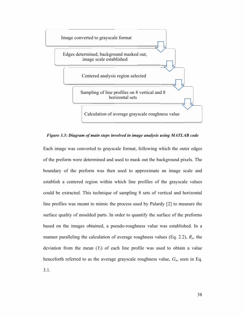
3.3.2 Image Analysis
The digital images obtained from this technique were then analysed using custom
code created for MATLAB computing software, as described in Figure 3.3.
E
of
bo
es
co
li
su
ba
m
de
he
3
Figure 3.3: D
Each image w
f the preform
oundary of
stablish a c
ould be extr
ne profiles w
urface qualit
ased on the
manner paral
eviation fro
enceforth re
.1.
Imag
Edg
Diagram of m
was converte
m were deter
the preform
entered regi
racted. This
was meant t
ty of moulde
images obt
leling the ca
m the mean
eferred to as
ge converted
ges determinimag
Cente
Sampl
Calc
main steps in
ed to graysc
rmined and
m was then
ion within w
technique o
to mimic the
ed parts. In
tained, a ps
alculation of
n (Yi) of ea
the average
d to grayscal
ned, backgroge scale estab
ered analysis
ling of line phor
culation of a
volved in ima
cale format,
used to mas
n used to ap
which line
of sampling
e process us
order to qua
seudo-roughn
f average ro
ach line pro
e grayscale
le format
ound maskedblished
s region sele
profiles on 8rizontal sets
average gray
age analysis u
following w
sk out the ba
pproximate
profiles of
8 sets of ve
ed by Palard
antify the su
ness value w
oughness val
ofile was us
roughness v
d out,
ected
8 vertical and
yscale roughn
using MATLA
which the ou
ackground pi
an image s
the graysca
ertical and h
dy [2] to me
urface of the
was establis
lues (Eq. 2.2
ed to obtain
value, Ga, se
d 8
ness value
38
AB code
uter edges
ixels. The
scale and
ale values
horizontal
easure the
preforms
shed. In a
2), Ra. the
n a value
een in Eq.

39
∑=n
iia Y
nG 1
Eq. 3.1
The values obtained were measured in units of grayscale intensity, and provide a
basis for comparing dry preforms to each other. Better overall surface quality
should exist in those preforms that demonstrate the lowest grayscale roughness
values, since the deviation from the mean should be smallest in cases where the
preform has more uniform light transmission. The complete custom MATLAB
image analysis code can be found in Appendix A.
3.4 Resin Transfer Moulding
The RTM processing and resin characteristics utilised in this section are those
developed by previous researchers and deemed to be optimal for the current
experimental setup [5].
3.4.1 Moulding Process
The manufacture of composite test panels was completed using an industrial
hydraulic press fitted with a flat steel mould incorporating a circulating water
heating system. Fibreglass preforms were placed within a 3.175 mm thick picture
frame with a 26 cm x 24 cm opening, as shown in Figure 3.4.
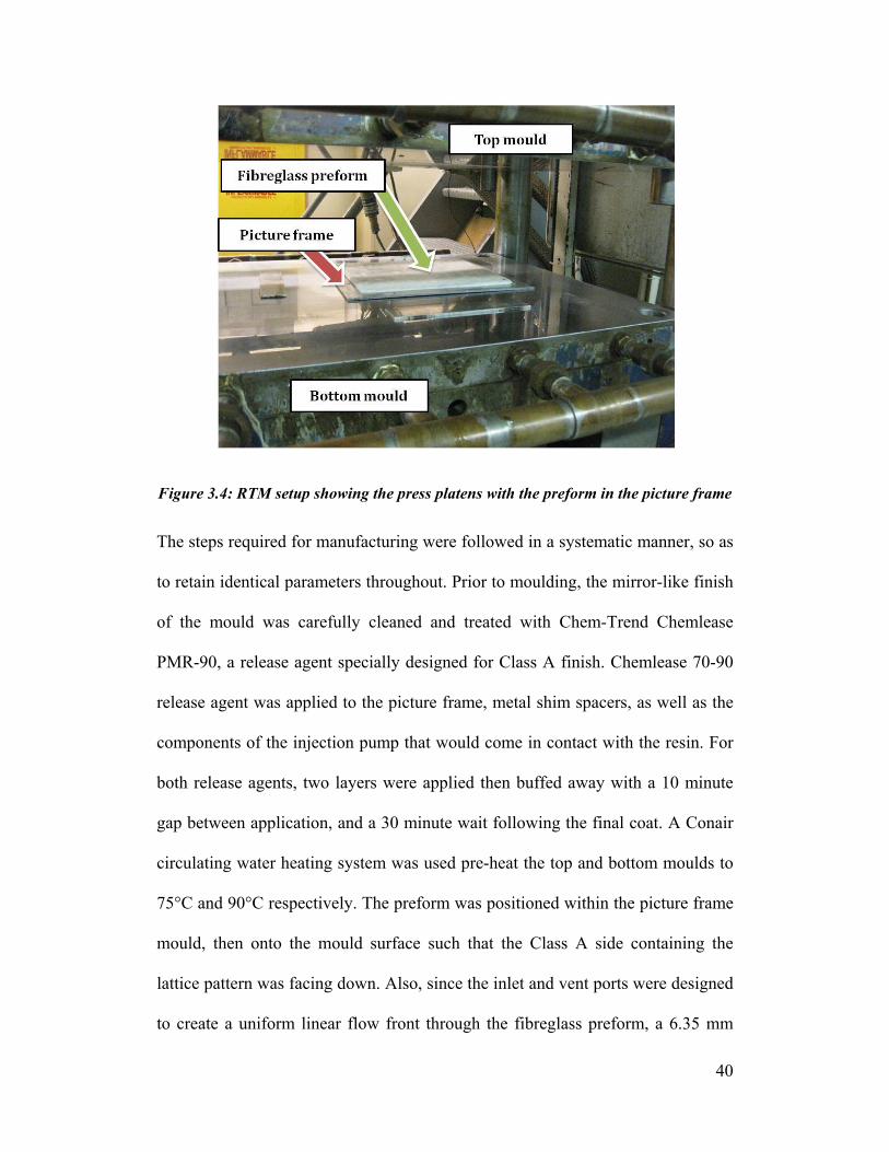
40
Figure 3.4: RTM setup showing the press platens with the preform in the picture frame
The steps required for manufacturing were followed in a systematic manner, so as
to retain identical parameters throughout. Prior to moulding, the mirror-like finish
of the mould was carefully cleaned and treated with Chem-Trend Chemlease
PMR-90, a release agent specially designed for Class A finish. Chemlease 70-90
release agent was applied to the picture frame, metal shim spacers, as well as the
components of the injection pump that would come in contact with the resin. For
both release agents, two layers were applied then buffed away with a 10 minute
gap between application, and a 30 minute wait following the final coat. A Conair
circulating water heating system was used pre-heat the top and bottom moulds to
75°C and 90°C respectively. The preform was positioned within the picture frame
mould, then onto the mould surface such that the Class A side containing the
lattice pattern was facing down. Also, since the inlet and vent ports were designed
to create a uniform linear flow front through the fibreglass preform, a 6.35 mm
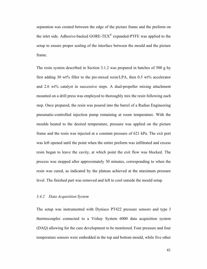
41
separation was created between the edge of the picture frame and the preform on
the inlet side. Adhesive-backed GORE-TEX® expanded-PTFE was applied to the
setup to ensure proper sealing of the interface between the mould and the picture
frame.
The resin system described in Section 3.1.2 was prepared in batches of 500 g by
first adding 30 wt% filler to the pre-mixed resin/LPA, then 0.5 wt% accelerator
and 2.6 wt% catalyst in successive steps. A dual-propeller mixing attachment
mounted on a drill press was employed to thoroughly mix the resin following each
step. Once prepared, the resin was poured into the barrel of a Radius Engineering
pneumatic-controlled injection pump remaining at room temperature. With the
moulds heated to the desired temperature, pressure was applied on the picture
frame and the resin was injected at a constant pressure of 621 kPa. The exit port
was left opened until the point when the entire preform was infiltrated and excess
resin began to leave the cavity, at which point the exit flow was blocked. The
process was stopped after approximately 30 minutes, corresponding to when the
resin was cured, as indicated by the plateau achieved at the maximum pressure
level. The finished part was removed and left to cool outside the mould setup.
3.4.2 Data Acquisition System
The setup was instrumented with Dynisco PT422 pressure sensors and type J
thermocouples connected to a Vishay System 6000 data acquisition system
(DAQ) allowing for the cure development to be monitored. Four pressure and four
temperature sensors were embedded in the top and bottom mould, while five other

42
temperature sensors were attached at various locations externally. An additional
pressure transducer was employed to observe the pressure maintained in the
injection pump. The live development of the pressure curves was monitored to
know when curing was complete, in addition to data being acquired at 10 samples
per second throughout the entire RTM processing.
Figure 3.5: Position of temperature (Ti) and pressure (Pi) sensors connected to DAQ and mounted on RTM press
T5 P5 T4
T3
P3
T1
P2
P1IN
OUTFlow
Direction
Runner – 6.35 mm thick
Fibreglass Preform
Picture Frame
P4
T2
T6
T7 Pump Pressure
Top Mould (Mid)
Top Mould (Edge)
Bottom Mould (Edge)
Other Sensors
T8
T9
Ambient
Ambient (Beside Press)

43
3.4.3 Mould Surface Finish
In order to verify the quality of the finish on the bottom mould, surface roughness
measurements were carried out using a Mitutoyo Surftest 401 Portable Tester.
Sets of profile scans were run at the four corners and centre of the area of interest.
The profilometer’s diamond stylus of radius 5 µm had a driving speed of 0.5
mm/s and a sampling rate of 400 points/s, allowing for values as small as 0.01 µm
to be read. The average roughness, Ra, measured with a cut-off wavelength of 2.5
mm had a mean value of 0.5 µm, with values ranging from 0.4 µm to 0.6 µm.
3.5 Surface Finish Measurement
For this research, each composite panel was first imaged using the ONDULO
system, following which a representative sample sized 80 mm x 80 mm was
identified for surface quality measurements.
3.5.1 ONDULO Measurements
The Visuol Technologies ONDULO system was utilised for the purpose of
imaging and qualifying the surface finish of manufactured composite panels. The
samples were placed upon a table positioned between a digital camera and a
projection screen in a darkened room, as seen in Figure 3.6.
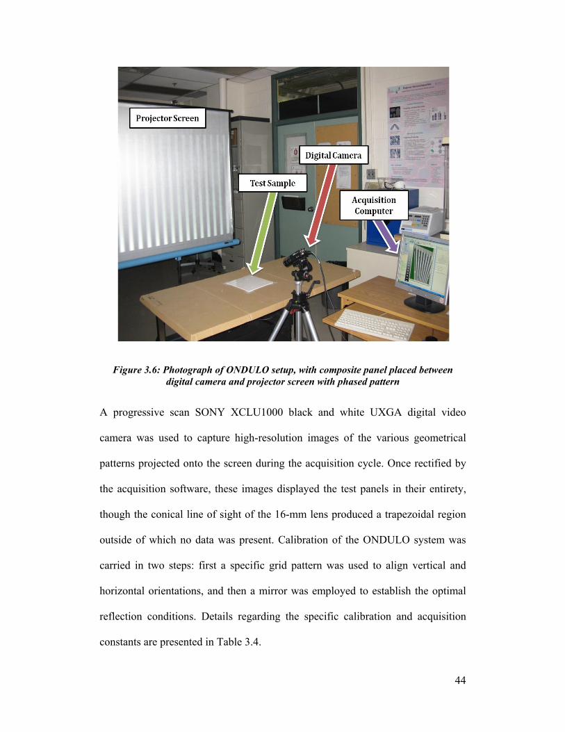
44
Figure 3.6: Photograph of ONDULO setup, with composite panel placed between digital camera and projector screen with phased pattern
A progressive scan SONY XCLU1000 black and white UXGA digital video
camera was used to capture high-resolution images of the various geometrical
patterns projected onto the screen during the acquisition cycle. Once rectified by
the acquisition software, these images displayed the test panels in their entirety,
though the conical line of sight of the 16-mm lens produced a trapezoidal region
outside of which no data was present. Calibration of the ONDULO system was
carried in two steps: first a specific grid pattern was used to align vertical and
horizontal orientations, and then a mirror was employed to establish the optimal
reflection conditions. Details regarding the specific calibration and acquisition
constants are presented in Table 3.4.
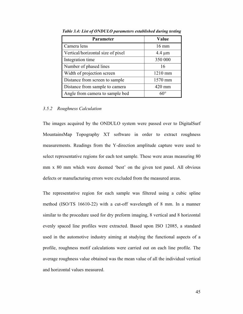
45
Table 3.4: List of ONDULO parameters established during testing
Parameter Value Camera lens 16 mm Vertical/horizontal size of pixel 4.4 µm Integration time 350 000 Number of phased lines 16 Width of projection screen 1210 mm Distance from screen to sample 1570 mm Distance from sample to camera 420 mm Angle from camera to sample bed 60°
3.5.2 Roughness Calculation
The images acquired by the ONDULO system were passed over to DigitalSurf
MountainsMap Topography XT software in order to extract roughness
measurements. Readings from the Y-direction amplitude capture were used to
select representative regions for each test sample. These were areas measuring 80
mm x 80 mm which were deemed ‘best’ on the given test panel. All obvious
defects or manufacturing errors were excluded from the measured areas.
The representative region for each sample was filtered using a cubic spline
method (ISO/TS 16610-22) with a cut-off wavelength of 8 mm. In a manner
similar to the procedure used for dry preform imaging, 8 vertical and 8 horizontal
evenly spaced line profiles were extracted. Based upon ISO 12085, a standard
used in the automotive industry aiming at studying the functional aspects of a
profile, roughness motif calculations were carried out on each line profile. The
average roughness value obtained was the mean value of all the individual vertical
and horizontal values measured.

46
3.6 Summary of Experimental Work
Fibreglass preforms manufactured according to the F3P method were obtained in
sheets sized 120 cm x 80 cm from Sotira Composites for testing. Using a 26 cm x
24 cm standard cutting template, three samples were prepared for each test set.
One session was needed to complete the imaging of all dry cut preforms for light
transmission. Next, the two preforms from each set deemed best by observation
were individually manufactured by RTM into test panels, with the processing
procedures remaining unchanged throughout and being carried out in a randomly
selected order. Finally, analysis was carried out to determine relative surface
finish quality, first by observation, then utilising the ONDULO system.

47
4 Results and Discussion
A description of the results and observations concerning the 16 test panels
manufactured follows. For reference, the samples will be labelled using “Set-
Test” as the format, therefore test 3-2 would refer to the second test sample from
Set 3. The outcome of work employing a novel preform imaging technique will
be discussed in Section 4.1. Details regarding RTM processing will be presented
in Section 4.2, before surface finish measurements are disclosed in Section 4.3.
Section 4.4 includes the analysis of variance for the results obtained, while
Section 4.5 discusses the relationship between the various outcomes.
4.1 Preform Imaging Technique
Photographs taken using the novel imaging fixture are described in Section 4.1.1,
following which the procedure used to obtain relevant data is discussed in Section
4.1.2.
4.1.1 Light Transmission Imaging
The light transmission imaging setup used for this work was designed to obtain
information regarding the overall quality of dry preforms prior to moulding. A
preform from Set 2 (Vf = 14%, Top Veil wt% = 15%) is shown imaged with the
Class A side facing up in Figure 4.1, and then facing down in Figure 4.2. It is
clear that the images obtained are not identical when photographed from either
side, but rather demonstrate a combination of darkness in areas where light is
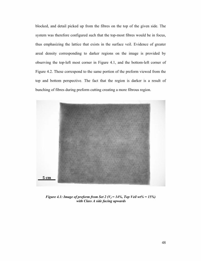
48
blocked, and detail picked up from the fibres on the top of the given side. The
system was therefore configured such that the top-most fibres would be in focus,
thus emphasizing the lattice that exists in the surface veil. Evidence of greater
areal density corresponding to darker regions on the image is provided by
observing the top-left most corner in Figure 4.1, and the bottom-left corner of
Figure 4.2. These correspond to the same portion of the preform viewed from the
top and bottom perspective. The fact that the region is darker is a result of
bunching of fibres during preform cutting creating a more fibrous region.
Figure 4.1: Image of preform from Set 2 (Vf = 14%, Top Veil wt% = 15%) with Class A side facing upwards
5 cm
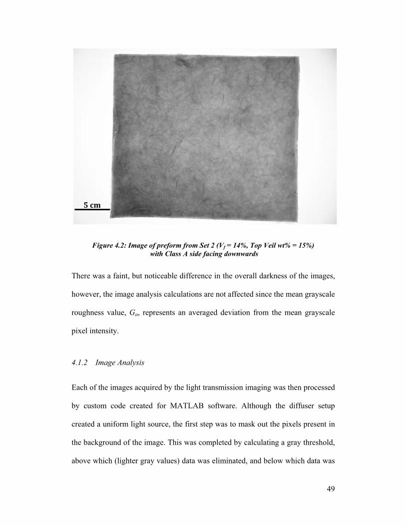
49
Figure 4.2: Image of preform from Set 2 (Vf = 14%, Top Veil wt% = 15%) with Class A side facing downwards
There was a faint, but noticeable difference in the overall darkness of the images,
however, the image analysis calculations are not affected since the mean grayscale
roughness value, Ga, represents an averaged deviation from the mean grayscale
pixel intensity.
4.1.2 Image Analysis
Each of the images acquired by the light transmission imaging was then processed
by custom code created for MATLAB software. Although the diffuser setup
created a uniform light source, the first step was to mask out the pixels present in
the background of the image. This was completed by calculating a gray threshold,
above which (lighter gray values) data was eliminated, and below which data was
5 cm
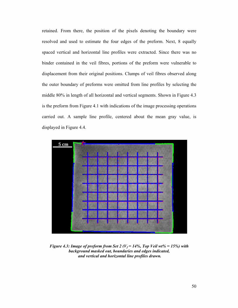
50
retained. From there, the position of the pixels denoting the boundary were
resolved and used to estimate the four edges of the preform. Next, 8 equally
spaced vertical and horizontal line profiles were extracted. Since there was no
binder contained in the veil fibres, portions of the preform were vulnerable to
displacement from their original positions. Clumps of veil fibres observed along
the outer boundary of preforms were omitted from line profiles by selecting the
middle 80% in length of all horizontal and vertical segments. Shown in Figure 4.3
is the preform from Figure 4.1 with indications of the image processing operations
carried out. A sample line profile, centered about the mean gray value, is
displayed in Figure 4.4.
Figure 4.3: Image of preform from Set 2 (Vf = 14%, Top Veil wt% = 15%) with background masked out, boundaries and edges indicated,
and vertical and horizontal line profiles drawn.
5 cm
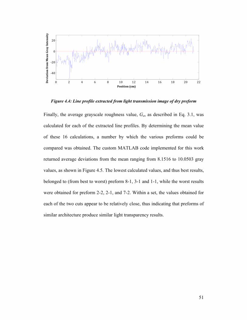
51
Figure 4.4: Line profile extracted from light transmission image of dry preform
Finally, the average grayscale roughness value, Ga, as described in Eq. 3.1, was
calculated for each of the extracted line profiles. By determining the mean value
of these 16 calculations, a number by which the various preforms could be
compared was obtained. The custom MATLAB code implemented for this work
returned average deviations from the mean ranging from 8.1516 to 10.0503 gray
values, as shown in Figure 4.5. The lowest calculated values, and thus best results,
belonged to (from best to worst) preform 8-1, 3-1 and 1-1, while the worst results
were obtained for preform 2-2, 2-1, and 7-2. Within a set, the values obtained for
each of the two cuts appear to be relatively close, thus indicating that preforms of
similar architecture produce similar light transparency results.
0 2 4 6 8 10 12 14 16 18 20 22
‐40
‐20
0
20
Position (cm)
Deviation from
Mean Gray Intensity
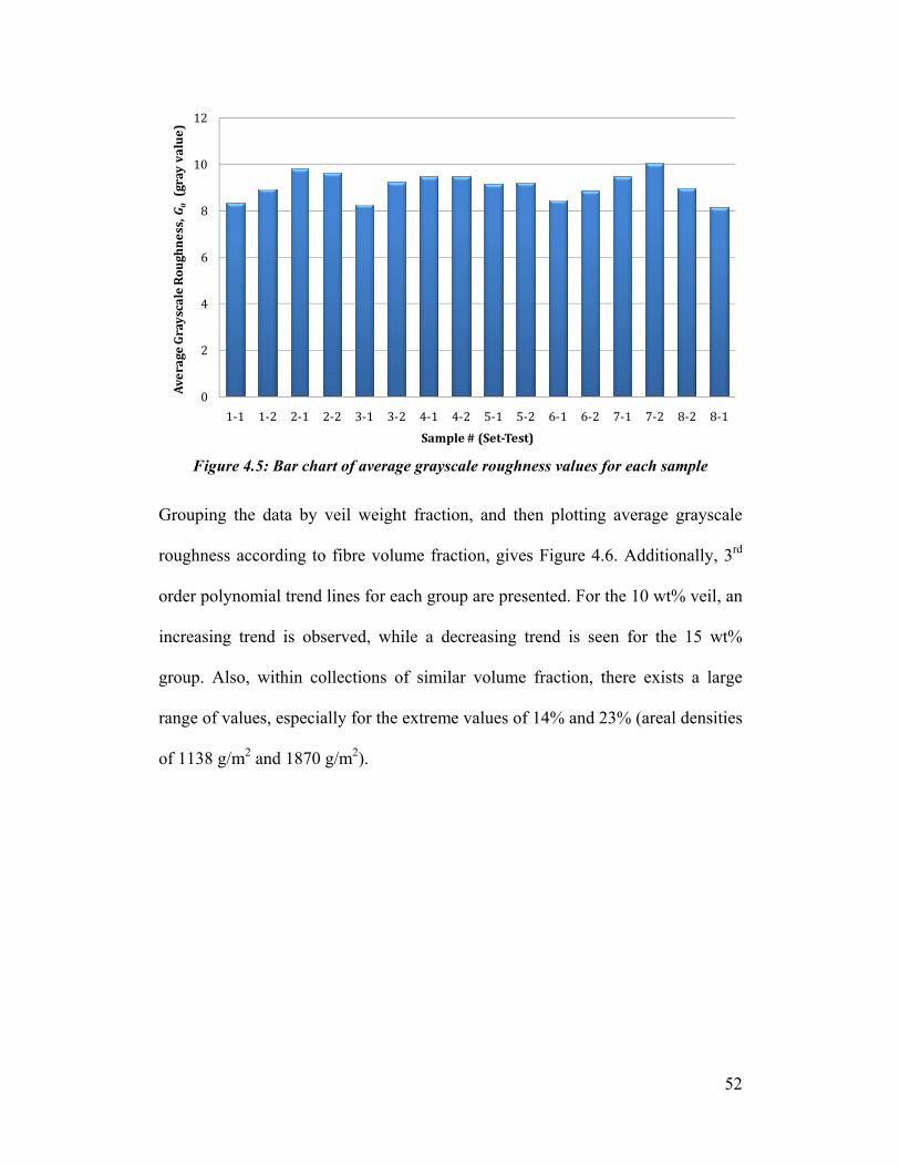
52
Figure 4.5: Bar chart of average grayscale roughness values for each sample
Grouping the data by veil weight fraction, and then plotting average grayscale
roughness according to fibre volume fraction, gives Figure 4.6. Additionally, 3rd
order polynomial trend lines for each group are presented. For the 10 wt% veil, an
increasing trend is observed, while a decreasing trend is seen for the 15 wt%
group. Also, within collections of similar volume fraction, there exists a large
range of values, especially for the extreme values of 14% and 23% (areal densities
of 1138 g/m2 and 1870 g/m2).
0
2
4
6
8
10
12
1‐1 1‐2 2‐1 2‐2 3‐1 3‐2 4‐1 4‐2 5‐1 5‐2 6‐1 6‐2 7‐1 7‐2 8‐2 8‐1
Average Grayscale Roughness, Ga(gray value)
Sample # (SetTest)
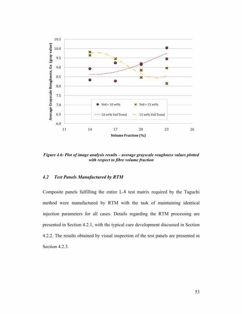
53
Figure 4.6: Plot of image analysis results – average grayscale roughness values plotted with respect to fibre volume fraction
4.2 Test Panels Manufactured by RTM
Composite panels fulfilling the entire L-8 test matrix required by the Taguchi
method were manufactured by RTM with the task of maintaining identical
injection parameters for all cases. Details regarding the RTM processing are
presented in Section 4.2.1, with the typical cure development discussed in Section
4.2.2. The results obtained by visual inspection of the test panels are presented in
Section 4.2.3.
6.0
6.5
7.0
7.5
8.0
8.5
9.0
9.5
10.0
10.5
11 14 17 20 23 26
Average Grayscale Roughness, Ga (gray value)
Volume Fraction (%)
Veil = 10 wt% Veil = 15 wt%
10 wt% Veil Trend 15 wt% Veil Trend
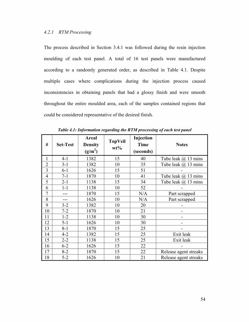
54
4.2.1 RTM Processing
The process described in Section 3.4.1 was followed during the resin injection
moulding of each test panel. A total of 16 test panels were manufactured
according to a randomly generated order, as described in Table 4.1. Despite
multiple cases where complications during the injection process caused
inconsistencies in obtaining panels that had a glossy finish and were smooth
throughout the entire moulded area, each of the samples contained regions that
could be considered representative of the desired finish.
Table 4.1: Information regarding the RTM processing of each test panel
# Set-Test Areal
Density (g/m2)
TopVeil wt%
InjectionTime
(seconds) Notes
1 4-1 1382 15 40 Tube leak @ 13 mins 2 3-1 1382 10 35 Tube leak @ 13 mins 3 6-1 1626 15 51 - 4 7-1 1870 10 41 Tube leak @ 13 mins 5 2-1 1138 15 34 Tube leak @ 13 mins 6 1-1 1138 10 52 - 7 --- 1870 15 N/A Part scrapped 8 --- 1626 10 N/A Part scrapped 9 3-2 1382 10 20 - 10 7-2 1870 10 21 - 11 1-2 1138 10 30 - 12 5-1 1626 10 30 - 13 8-1 1870 15 25 - 14 4-2 1382 15 25 Exit leak 15 2-2 1138 15 25 Exit leak 16 6-2 1626 15 22 - 17 8-2 1870 15 22 Release agent streaks 18 5-2 1626 10 21 Release agent streaks

55
RTM injections #7 and #8 were parts that needed to be scrapped due to
incomplete infiltration of the fibreglass preforms. This was due to the calcium
carbonate used as filler in the resin mixture, which ran out after six tests and was
replaced by an older batch which had clearly undergone enough of a chemical
change to limit the flow of the resin. For injections thereafter, a newly purchased
batch of calcium carbonate was used, as evidenced by the lower time required for
the resin to infiltrate the preform and flow out the exit.
In the case of injections #1, #2, #4, and #5, the use of polyethylene tubing
incorrectly rated for the temperature and pressure needs of RTM processing led to
a rupture in the inlet tubing at the 13 minute mark, corresponding to when the
resin was undergoing volumetric expansion caused by the LPAs. Since preform
infiltration was already complete, the effect was seen in the form of ripples or
waviness on the finished panel, as opposed to dry sections. These defects,
however, were limited to certain regions and did not appear to affect the rest of
the panel, which exhibited the desired consistent and glossy finish. In a similar
manner, incorrect sealing of the exit port caused leaks which produced the same
regional ripples in injections #14 and #15. It should be noted that the situation
regarding inadequate polyethylene tubing was rectified by replacing these
components with a more robust set of nylon tubing.
In the case of injections #17 and #18, a saturated cloth used for the application
and buffing of release agent caused streaks on the mould, which at the time were
imperceptible, to produce streak marks on the finished panels. Again, these
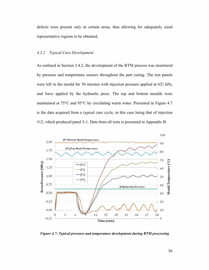
56
defects were present only in certain areas, thus allowing for adequately sized
representative regions to be obtained.
4.2.2 Typical Cure Development
As outlined in Section 3.4.2, the development of the RTM process was monitored
by pressure and temperature sensors throughout the part curing. The test panels
were left in the mould for 30 minutes with injection pressure applied at 621 kPa,
and force applied by the hydraulic press. The top and bottom moulds were
maintained at 75°C and 95°C by circulating warm water. Presented in Figure 4.7
is the data acquired from a typical cure cycle, in this case being that of injection
#12, which produced panel 5-1. Data from all tests is presented in Appendix B.
Figure 4.7: Typical pressure and temperature development during RTM processing

57
The plot shows the temperature maintained on the top and bottom moulds, though
the curve is in a sinusoidal form. This is due to the warm water which was
circulated into the moulds warm, cooled, and then replaced by new warm water
approximately every 3 minutes. The four pressure sensors embedded into the
moulds (as seen in Figure 3.5) measured the resin pressure throughout the cure
development. The values were zeroed with the mould cavity closed and only the
dry preform present. Upon injection, the pressure mounts to approximately 500
kPa and stays there for about 6 minutes, at which point resin volumetric shrinkage
begins to set in. Work by Raja [5], observed that LPAs remained inactive until a
degree-of-cure of approximately 0.5, following which expansion of the
thermoplastic particles starts. This expansion is seen after about 9 minutes in the
cure development shown in Figure 4.7, and continues until the resin pressure
begins to level off after 20 minutes. Again, sinusoidal curves are seen and can be
attributed to the circulating water, though this time in the case of the pressure
values. As the resin pressure stabilizes, it is clear there is a cure gradient at
different sensor locations. This phenomenon can be accounted for by the fact that
the cure starts at the vent port and travels towards the injection port, as detailed by
Raja [5]. It is of interest to note that rapid expansion of the resin is occurring at
the 13 minute mark, which corresponds to the time when several of the injection
tests had ruptures in the polyethylene tubing. It is evident that in addition to the
elevated processing temperature, the internal pressure of nearly 1 MPa caused the
tubing to break.

58
4.2.3 Visual Inspection of Surface Finish
With the objective of completing an initial investigation into the surface finish
quality of the manufactured test panels, a method of visual inspection was
employed. The region containing the most desirable surface finish within each
panel was compared side by side with each of the others until an overall ranking
was obtained. The decision of whether a panel was better or worse than another
was based upon which one appeared to be more flat, smooth and exempt of
undesirable waviness, as well as the desire to have a more mirror-like surface.
Table 4.2 below categorizes the results and gives a description of the qualities
observed within each category.
Table 4.2: Quality of surface finish observed in test panels
Quality Test Panels Description
Best 2-1, 6-1, 7-1 Glossy, mirror-like finish.
6-2, 8-1, 5-1 Glossy finish.
Worst 2-2, 5-2, 8-2, 3-2, 1-1, 3-1, 7-2, 4-1, 1-2, 4-2 Semi-gloss finish.
In the case of the best panels, the fibre lattice pattern was clearly visible as an
image on the surface, though the texture was not affected. Meanwhile, the image
of the fibre lattice pattern was completely obscured in the worst panels.
It is interesting to note that, by observation, preforms within the same
manufactured set (e.g. Set 2 & 7) provided samples falling in both the best and
worst category of surface finish quality. One would expect preforms cut from the
same sheet to output similar surface finish results if all other factors remained

59
constant. The possibility that the fibre areal density and surface veil thickness are
weak factors contributing the surface finish quality appears to be the likely
explanation for such results. Thus, even slight variations in dominant
manufacturing factors such as injection pressure could have a larger effect on
surface quality than variations in fibre areal density and surface veil thickness.
4.3 ONDULO Measurements
With the aim of gaining a more quantitative measure of the surface finish, each of
the test panels was imaged using the ONDULO system, following which analysis
was carried out utilising MountainsMap topography software. Obtained from this
exercise were roughness values used to compare the quality of each finished test
panel.
4.3.1 ONDULO Measurement System
The technique and parameters outlined in Section 3.5.1 were applied for the
purpose of imaging each of the 16 test panels manufactured for this project. An
image of test panel 6-1 is shown in Figure 4.8. As mentioned, the 16-mm lens
provided a trapezoidal viewport of each panel due to the conical point-of-view of
the digital camera. The area outside this viewport captured by the system is
indicated as ‘NM’ – not measured. A noticeable gradient from light to dark
appeared from the top to the bottom of the image. This is an artefact of the
ONDULO technique that needed to be removed by the image processing
software. The images appeared most clearly in the high-lustre regions, and
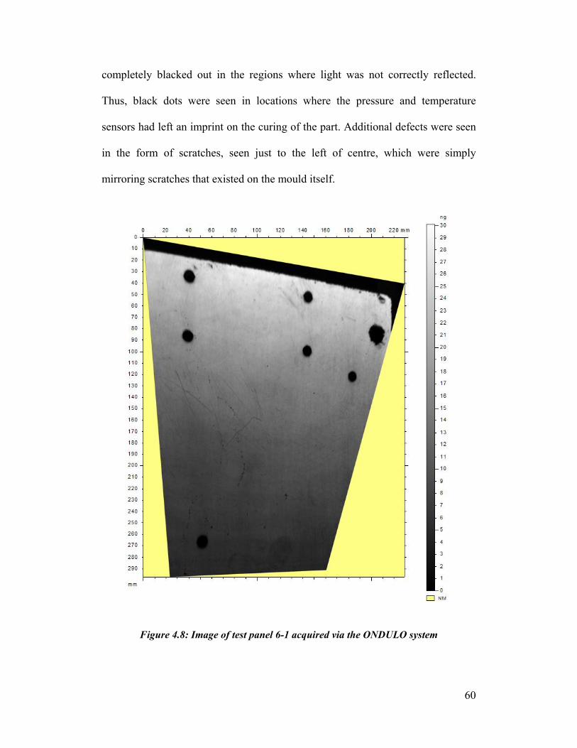
60
completely blacked out in the regions where light was not correctly reflected.
Thus, black dots were seen in locations where the pressure and temperature
sensors had left an imprint on the curing of the part. Additional defects were seen
in the form of scratches, seen just to the left of centre, which were simply
mirroring scratches that existed on the mould itself.
Figure 4.8: Image of test panel 6-1 acquired via the ONDULO system
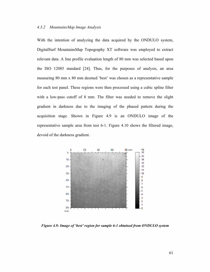
61
4.3.2 MountainsMap Image Analysis
With the intention of analyzing the data acquired by the ONDULO system,
DigitalSurf MountainsMap Topography XT software was employed to extract
relevant data. A line profile evaluation length of 80 mm was selected based upon
the ISO 12085 standard [24]. Thus, for the purposes of analysis, an area
measuring 80 mm x 80 mm deemed ‘best’ was chosen as a representative sample
for each test panel. These regions were then processed using a cubic spline filter
with a low-pass cutoff of 8 mm. The filter was needed to remove the slight
gradient in darkness due to the imaging of the phased pattern during the
acquisition stage. Shown in Figure 4.9 is an ONDULO image of the
representative sample area from test 6-1. Figure 4.10 shows the filtered image,
devoid of the darkness gradient.
Figure 4.9: Image of ‘best’ region for sample 6-1 obtained from ONDULO system
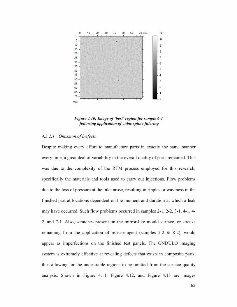
62
Figure 4.10: Image of ‘best’ region for sample 6-1 following application of cubic spline filtering
4.3.2.1 Omission of Defects
Despite making every effort to manufacture parts in exactly the same manner
every time, a great deal of variability in the overall quality of parts remained. This
was due to the complexity of the RTM process employed for this research,
specifically the materials and tools used to carry out injections. Flow problems
due to the loss of pressure at the inlet arose, resulting in ripples or waviness in the
finished part at locations dependent on the moment and duration at which a leak
may have occurred. Such flow problems occurred in samples 2-1, 2-2, 3-1, 4-1, 4-
2, and 7-1. Also, scratches present on the mirror-like mould surface, or streaks
remaining from the application of release agent (samples 5-2 & 8-2), would
appear as imperfections on the finished test panels. The ONDULO imaging
system is extremely effective at revealing defects that exists in composite parts,
thus allowing for the undesirable regions to be omitted from the surface quality
analysis. Shown in Figure 4.11, Figure 4.12, and Figure 4.13 are images
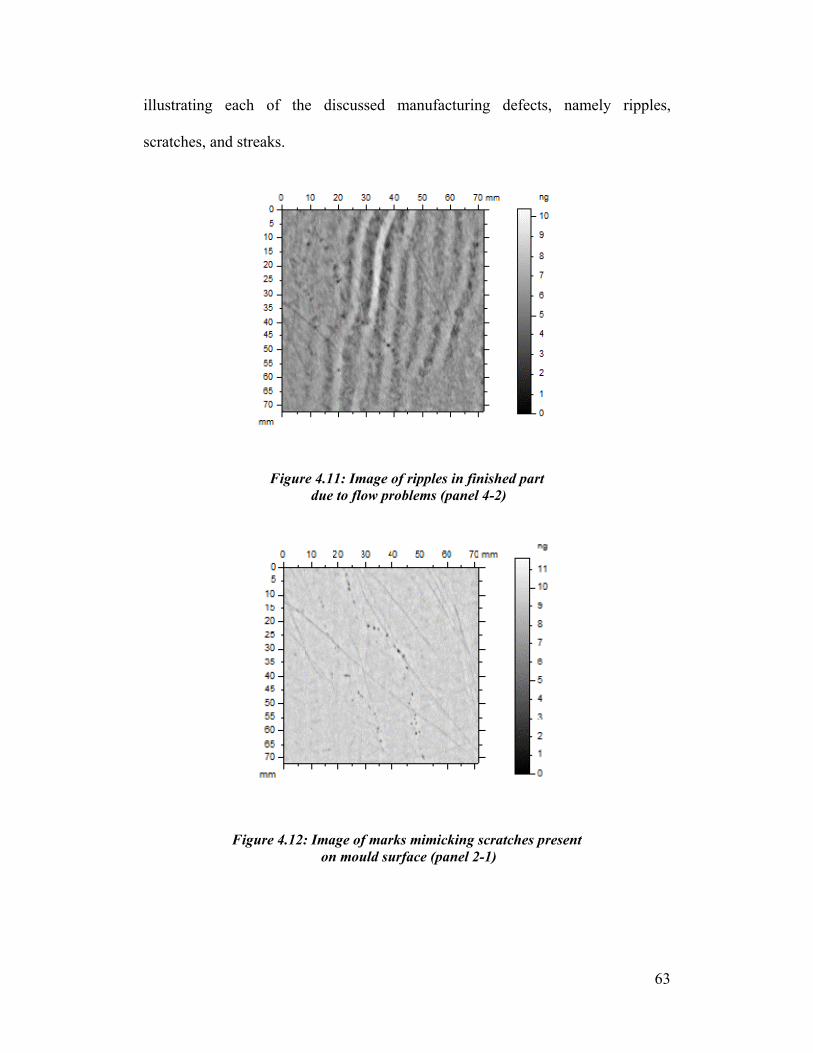
63
illustrating each of the discussed manufacturing defects, namely ripples,
scratches, and streaks.
Figure 4.11: Image of ripples in finished part due to flow problems (panel 4-2)
Figure 4.12: Image of marks mimicking scratches present on mould surface (panel 2-1)
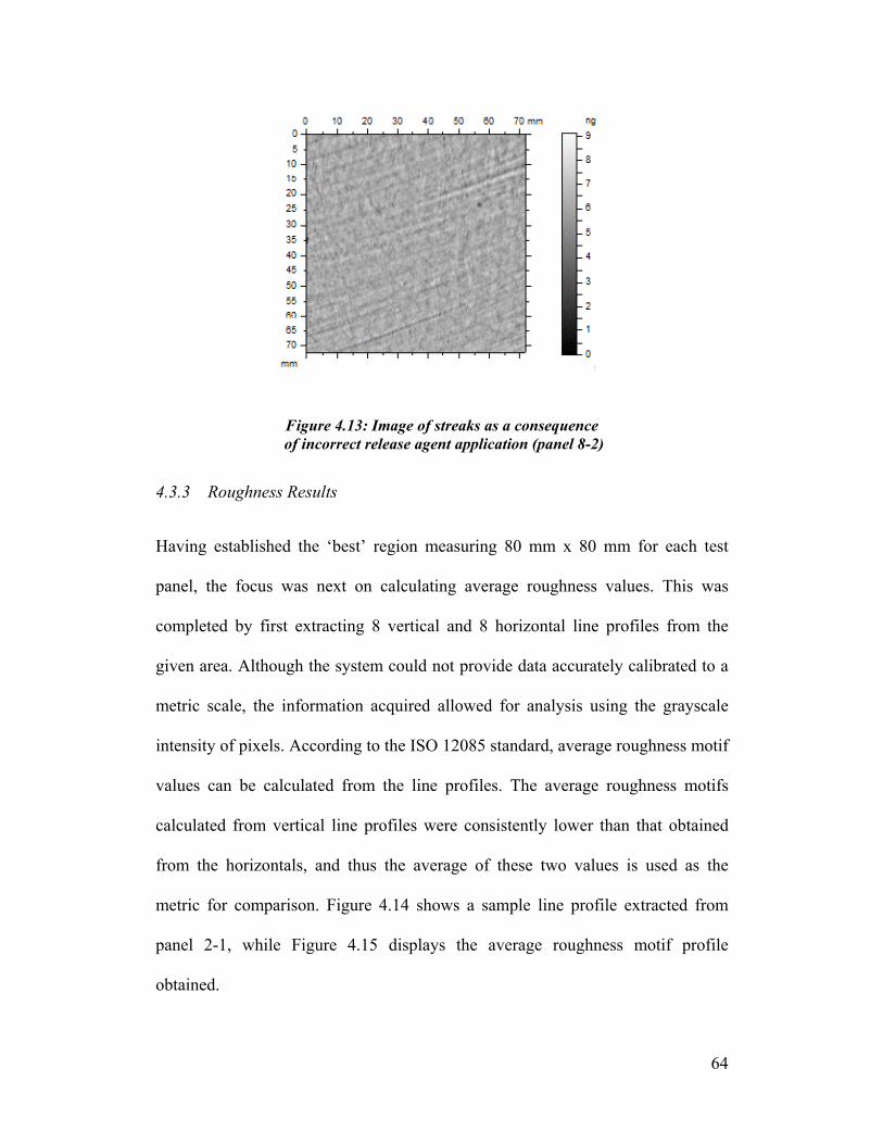
64
Figure 4.13: Image of streaks as a consequence of incorrect release agent application (panel 8-2)
4.3.3 Roughness Results
Having established the ‘best’ region measuring 80 mm x 80 mm for each test
panel, the focus was next on calculating average roughness values. This was
completed by first extracting 8 vertical and 8 horizontal line profiles from the
given area. Although the system could not provide data accurately calibrated to a
metric scale, the information acquired allowed for analysis using the grayscale
intensity of pixels. According to the ISO 12085 standard, average roughness motif
values can be calculated from the line profiles. The average roughness motifs
calculated from vertical line profiles were consistently lower than that obtained
from the horizontals, and thus the average of these two values is used as the
metric for comparison. Figure 4.14 shows a sample line profile extracted from
panel 2-1, while Figure 4.15 displays the average roughness motif profile
obtained.

65
Figure 4.14: Line profile extracted from filtered ‘best’ region in test panel 2-1
Figure 4.15: Roughness motif for line profile of filtered ‘best’ region in test panel 2-1
Shown in Figure 4.16, the results ranged from 0.234 to 0.413 pixels, with the best
values seen in samples 6-2, 4-2, and 2-2, and worst in 8-1, 5-1, and 5-2. This
value of grayscale pixel intensity, however, cannot be compared directly with that
from the photographs of the dry preforms since each employs a different optical
technique. The large variation indicated by the error bars can be explained by the
discrepancy between the average vertical and horizontal values.
ng
-2
-1.5
-1
-0.5
0
0.5
1
1.5
0 5 10 15 20 25 30 35 40 45 50 55 60 65 70 mm
Length = 72 mm Pt = 2.5 ng Scale = 4 ng
ng
-2
-1.5
-1
-0.5
0
0.5
1
1.5
0 5 10 15 20 25 30 35 40 45 50 55 60 65 70 mm
R = 0.359 ng AR = 0.332 mm Rx = 1.48 ng Pt = 2.5 ng

66
Figure 4.16: Bar chart of average roughness values from ONDULO for each sample
Figure 4.17 shows the average roughness motifs plotted according to fibre volume
fraction. Again, sets are regrouped by surface veil weight fraction and 3rd order
polynomial trend lines are included. All values except for those corresponding to
the 20% fibre volume fraction are seen to be between 0.30 and 0.35 gray intensity.
At the 20% mark, all four test panels appear to have produced very different
results, with the larger veil wt% resulting in a smaller roughness and therefore
better finish.
0.00
0.10
0.20
0.30
0.40
0.50
1‐1 1‐2 2‐1 2‐2 3‐1 3‐2 4‐1 4‐2 5‐1 5‐2 6‐1 6‐2 7‐1 7‐2 8‐2 8‐1
Average Roughness, Ra(gray value)
Sample # (SetTest)
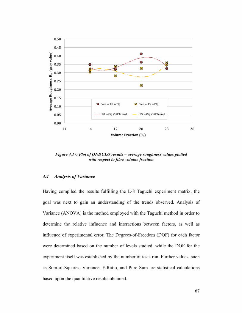
67
Figure 4.17: Plot of ONDULO results – average roughness values plotted with respect to fibre volume fraction
4.4 Analysis of Variance
Having compiled the results fulfilling the L-8 Taguchi experiment matrix, the
goal was next to gain an understanding of the trends observed. Analysis of
Variance (ANOVA) is the method employed with the Taguchi method in order to
determine the relative influence and interactions between factors, as well as
influence of experimental error. The Degrees-of-Freedom (DOF) for each factor
were determined based on the number of levels studied, while the DOF for the
experiment itself was established by the number of tests run. Further values, such
as Sum-of-Squares, Variance, F-Ratio, and Pure Sum are statistical calculations
based upon the quantitative results obtained.
0.00
0.05
0.10
0.15
0.20
0.25
0.30
0.35
0.40
0.45
0.50
11 14 17 20 23 26
Average Roughness, Ra(gray value)
Volume Fraction (%)
Veil = 10 wt% Veil = 15 wt%
10 wt% Veil Trend 15 wt% Veil Trend

68
4.4.1 Dry Preform Image Analysis
ANOVA was carried out based on the results obtained from the image analysis of
the dry preforms. The influence of the fibre volume fraction was larger than that
of the veil weight fraction; however, both were dwarfed by the influence of the
error term of the experiments, as seen in Table 4.3. The minimum MSD would
imply that Set 8 (Vf = 23%, Veil wt% = 15%) is the optimal condition, while the
trends within each factor would point to Set 5 (Vf = 20%, Veil wt% = 10%) as the
optimal configuration.
Table 4.3: ANOVA for image analysis data, based on design factors
# Preform Vf Veil Wf Error Total Factor DOF (f) 3 1 11 15 Sum of Squares (S) 0.169 0.003 4.659 4.831 Variance (V) 0.056 0.003 0.424 0.322 F-Ratio (F) 0.133 0.006 - - Pure Sum (S') -1.1 -0.42 - - Percent Influence (P) 0% 0% 100% 100%
4.4.2 ONDULO Measurements
Similarly, the ANOVA for the results obtained from the ONDULA system
showed that the error term has a dominant influence on the experiment. The veil
thickness represented 11% of the influence, while the fibre volume fraction had
no influence, and the error/other factors filled the remaining 89%. A slight
increase in roughness was observed as fibre volume fraction was increased, and
veil size is decreased. Thus, the optimal conditions according to ANOVA are seen
in Set 4 (Vf = 17%, Veil wt% = 15%), while the minimum MSD occurs in Set 6

69
(Vf = 20%, Veil wt% = 15%). Table 4.4 displays the ANOVA results according to
the design factors studied in this experiment.
Table 4.4: ANOVA for ONDULO data, based on design factors
# Preform Vf Veil Wf Error Total Factor DOF (f) 3 1 11 15 Sum of Squares (S) 0.002 0.004 0.018 0.024 Variance (V) 5E-04 0.004 0.002 0.002 F-Ratio (F) 0.318 2.6 - - Pure Sum (S') 0 0.003 - - Percent Influence (P) 0% 11% 89% 100%
4.4.3 Discussion of ANOVA Results
Although the use of ANOVA has allowed for the determination of ‘optimal
conditions’, it is apparent that the variability over the range of fibre volume
fractions and surface veil weight fractions play a very slight role in the quality of
a composite part’s surface finish. In the process of manufacturing these parts, a
certain intuition regarding the influence of various factors was developed thanks
to the hands-on experience gained. The error term included in the ANOVA
combines all uncontrollable and excluded factors, as well as any experimental
error. Thus, when the error represents an extremely large percent influence in the
experiment, it means that the process is too sensitive to the influence of
uncontrollable factors and the samples have a large inherent variability [21].
Based upon the chosen evaluation technique, the results obtained indicate that
fibre volume fraction and surface veil thickness have little to no influence on the
surface finish quality.

70
4.5 Correlation of Results
One of the main objectives of this work was to determine the relationship between
quality of fibreglass preforms and surface finish of test panels manufactured by
RTM. By observing the large disparity between the set rankings of surface quality
for each of the two methods, it is evident that there is no apparent relationship
between the results obtained from the image analysis and those from the
ONDULO system. One would expect the best results from the image analysis to
correspond to the moulded samples with the best surface finish in order for a
correlation to be drawn. This is not seen either by observation or using the
ONDULO measurement technique. The implication is that although the analysis
carried out in both cases may be acceptable, no conclusions can be drawn prior to
moulding with respect to the ability to predict which preforms will result in
superior surface quality.
71
5 Conclusions
The goal of this work was to study the effect of preform variability on the surface
finish of Class A composite parts manufactured by RTM. This was accomplished
by first determining preform characteristics of interest, then by establishing a set
of experiments which allowed for the investigation of variability. Next, the quality
of dry preforms was studied both prior to, and following RTM processing.
Finally, ANOVA was employed to understand the influence of the factors studied.
The following details, as they pertain to the initial objectives of this project, can
be concluded upon:
1. Preform characteristics: Although F3P preform material selection and
machine parameters are of interest, fibreglass areal density and top veil
weight fraction were selected for further study. A range of 1138 g/m2 to
1870 g/m2 was chosen for areal density, while 10 wt% and 15 wt% top
veils were also picked for study.
2. Qualify dry preforms: A novel technique whereby the light transmitted
through dry preforms is photographed was utilised. Acquired images were
analysed in order to obtain average grayscale roughness values which
quantified the consistency of the preform surface.
3. Surface finish characterisation: Composite test panels were manufactured
by RTM, following which surface finish was characterised. This was
completed first by visual inspection, then by making use of the ONDULO
surface measurement system.

72
4. Relate results to surface finish: The results of the Taguchi method,
according to ANOVA, demonstrated that surface finish quality is
dominated by factors other than fibre areal density and surface veil
thickness. No relation was observed between the quality of the preforms
prior to and following moulding.
Based on the experimental techniques employed, the findings in this thesis
suggest that small variations in preform fibre volume fraction and top veil
thickness have no significant effect on the surface finish of ‘Class A’ composites
parts manufactured by RTM.
5.1 Future Work
Further work is required to verify the accuracy of the optical methods used for
imaging prior to and following moulding. The results obtained from a contact
profilometer could be compared to the ONDULO results to determine to what
extent the fibre lattice visible in the surface veil actually affects surface finish.
Also, it is of interest to study the average roughness motifs obtained within
several different ranges of wavelengths to verify that the appropriate waviness
components have been removed from the surface texture profiles.
Finally, it is of interest to understand the importance of micro-structural elements
in the fiberglass preform. The effect of the lattice patterns included on the Class A
side of the preforms, as well as the diameter and length of fibres should be
addressed in order to qualify their contribution to surface finish.
73
6 References
[1] Tucker, N., Lindsey, Kevin, 2002, An Introduction to Automotive
Composites, Rapra Technology Limited, Shawbury, U.K.
[2] Palardy, G., 2007, "Resin Volumetric Changes and Surface Finish
Characterization of Composite Automotive Panels," Master's Thesis McGill
University, Montréal, Qc.
[3] Black, S., 2008, "High-Volume Preformance for Automotive Application,"
Gardner Publications Inc.
[4] Potter, K., 1997, Resin Transfer Moulding, Chapman & Hall.
[5] Raja, M. H., 2005, "Experimental Optimization of Process Parameters to
Obtain Class a Surface Finish in Resin Transfer Molding Process," PhD Thesis
McGill University, Montreal, Qc.
[6] Wood, K., 2008, "Automotive Composites: Taking Subjectivity out of Class a
Surface Evaluation," Composites Technology.
[7] Karbhari, V. M. S., S.G.; Steenkamer, D.A.; Wilkins, D.J., 1992, "Effect of
Material, Process, and Equipment Variables on the Performance of Resin Transfer
Moulded Parts," Composites Manufacturing, 3(3), pp. 143-152.
[8] Dutiro, C., 1995, "Factors Affecting Surface Finish of Rtm Products,"
MSc(Eng.) Imperial College of Science and Technology and Medicine, UK.
[9] Dutiro, C. A., R.N., 1997, "Factors Controlling Surface Finish in Resin
Transfer Molding," SAMPE Journal, 33(5), pp. 19-23.
[10] Bayldon, J. M., 1996, "An in-Depth Study of Surface Finish in Resin
Transfer Moulding," MSc(Eng.) Imperial College of Science and Technology and
Medicine.
[11] Palardy, G.; Hubert, P.; Haider, M.; Lessard, L., 2008, "Optimization of Rtm
Processing Parameters for Class a Surface Finish," Composites: Part B, 39(pp.
1280-1286.
74
[12] Palardy, G., Hubert, P., 2007, "Effect of Painting Process on the Surface
Finish of Rtm Composite Car Body Panels," Paris, France.
[13] Haider, M., Hubert, P.; Lessard, L., 2007, "Cure Shrinkage Characterization
and Modeling of a Polyester Resin Containing Low Profile Additives,"
Composites: Part A, 38(pp. 994-1009.
[14] Devries, J. E., 2007, "Title," Wayne State University.
[15] Chavka, N. G. D., J.S., Kleven, E.D., 2001, "F3p Fiber Preforming for the
Aston Martin Vanquish," Proc. 2001 SAMPE Europe Int'l Conference, Paris.
[16] Harper, L. T. T., T.A.; Warrior, N.A.; Dahl, J.S.; Rudd, C.D., 2006,
"Characterisation of Random Carbon Fibre Composites from a Directed Fibre
Preforming Process: Analysis of Microstructural Parameters," Composites: Part
A, 37(pp. 2136-2147.
[17] Dahl, J. D., M.; Steenmaker, D., 2004, "Processing and Performance of
Chopped, Glass-Fiber-Reinforced Rtm Composites."
[18] Bebamzadeh, A. A., A.R.A.; Haukaas, T.; Vaziri, R.; Poursatip, A., 2005,
"Probabilistic and Sensitivity Analysis of Surface Waviness of Rtm Manufactured
Automotive Body Parts."
[19] Personal Communication with Kendall, K., Aston Martin.
[20] Fisher, R. A., 1993, Statistical Methods, Experimental Design, and Scientific
Inference, Oxford University Press, Oxford, U.K.
[21] Roy, R. K., 2001, Design of Experiments Using the Taguchi Approach: 16
Steps to Product and Process Improvement, Wiley-Interscience, USA.
[22] Ansi/Asme, 1985, "B46.1: Surface Texture, Surface Roughness, Waviness
and Lay."
[23] Mainsah, E. G., J.A.; Chetwynd, D.G., 2001, Metrology and Properties of
Engineering Surfaces, Kluwer Academic Publishers, The Netherlands.
[24] Digitalsurf, 2008, "Mountainsmap: User Help Manual."
75
[25] Whitefield, R. J., "Non-Contact Optical Profilometer," Applied Optics,
14(10), pp. 2480-2485.
[26] Vorburger, T. V. R., J., 1990, Surface Finish Metrology Tutorial,
Gaithersburg, MD.
[27] Techlab, 2002, Ondulo: L'analyse De L'aspect De Surface - Manuel
D'utilisation, Metz, France.
[28] Debolt, M. A., 2004, "Surface Finish Evaluation Method for Class a
Composite Substrates."
[29] Iso, "Surface Texture: Profile Method - Rules and Procedures for the
Assessment of Surface Texture."
[30] Schubel, P. J. W., Nicholas A.; Kendall, Kenith N.; Rudd, Chris D., 2006,
"Characterisation of Thermoset Laminates for Cosmetic Automotive
Applications: Part I - Surface Characterisation," Composites: Part A, 37(pp. 1734-
1746.
[31] Gan, M., "Understanding and Improving the Performance of Advanced
Composites through Modelling the Effect of Material Variability."

76
7 Appendix A
7.1 Custom MATLAB Image Analysis Code
areal_density.m
% areal_density.m -- by Ronnie Lawand % ----------------------------------------------- % Used to analyse fiberglass preform images clc; clear all; close all; fprintf('\n'); fprintf('PREFORM IMAGE ANALYSIS\n'); fprintf('----------------------\n'); fprintf(' Ronnie Lawand - 2009 \n'); fprintf('----------------------\n'); fprintf('\n'); fprintf('## -- File Name -- Scale Rough \n'); % Import image, convert to grayscale [N, T] = xlsread('list.xlsx'); Text = cellstr(T); Set8 = Text(:,4); Images = [Set8]; % Show plots? -- No: for batch runs print = 1; for pic = 1:length(Images) clear vLP hLP File = char(Images(pic)); rgb = imread(File); if print==0 fprintf('%2.0i -- %s -- ',pic,char(Images(pic))); end % Convert to gray, create binary image gray = rgb2gray(rgb); level = graythresh(gray); bin = ~im2bw(gray,level); % Determine an initial point, find boundary dim = size(bin); col = round(dim(2)/4); row = find(bin(:,col),1); boundary = bwtraceboundary(bin,[row, col],'E'); % Masked images of preform and background

77
bipreform = roipoly(gray,boundary(:,2),boundary(:,1)); preform = immultiply(gray,bipreform); % mask1 = immultiply(gray,~bipreform); % background = immultiply(mask1,~bin); % Show binary image and boundary of preform if print==1 figure1=figure; imshow(preform); hold on; plot(boundary(:,2),boundary(:,1),'g','LineWidth',3); plot(col,row,'MarkerFaceColor','r','MarkerSize',20,'Marker','pentagram'); end % \\\\\\\\\ DETERMINE LINE PROFILE \\\\\\\\\ % Determine and plot each of the column lines for c = 1:3 cLP_col(c) = round(dim(2)*c/4); % Picks column to use cLP_start(c) = find(bin(:,cLP_col(c)),1,'first'); % Finds start of column cLP_end(c) = find(bin(:,cLP_col(c)),1,'last'); % Finds end of column if print==1 plot(cLP_col(c),cLP_start(c),'MarkerFaceColor','r','MarkerSize',5,'Marker','o'); plot(cLP_col(c),cLP_end(c),'MarkerFaceColor','r','MarkerSize',5,'Marker','o'); end end % Determine and plot each of the row lines for r = 1:3 rLP_row(r) = round(dim(1)*r/4); rLP_start(r) = find(bin(rLP_row(r),:),1,'first'); rLP_end(r) = find(bin(rLP_row(r),:),1,'last'); if print==1 plot(rLP_start(r),rLP_row(r),'MarkerFaceColor','r','MarkerSize',5,'Marker','o'); plot(rLP_end(r),rLP_row(r),'MarkerFaceColor','r','MarkerSize',5,'Marker','o'); end end vFirst = round(mean(cLP_start)); vLast = round(mean(cLP_end)); vLength = vLast - vFirst; % Can be used for approximate sizing (vertical) hFirst = round(mean(rLP_start)); hLast = round(mean(rLP_end)); hLength = hLast - hFirst; % Can be used for approximate sizing (horizontal) vx = round(hFirst+hLength*(0.15:0.1/1:0.85)); vy = vFirst+round(vLength*0.1):vLast-round(vLength*0.1); for i = 1:length(vx) for j = 1:length(vy) if print==1 plot(vx(i),vy(j),'MarkerFaceColor','r','MarkerSize',2,'Marker','o'); end vLP(j,i) = preform(vy(j),vx(i)); end end

78
hy = round(vFirst+vLength*(0.15:0.1/1:0.85)); hx = hFirst+round(hLength*0.1):hLast-round(hLength*0.1); for i = 1:length(hy) for j = 1:length(hx) if print==1 plot(hx(j),hy(i),'MarkerFaceColor','r','MarkerSize',2,'Marker','o'); end hLP(j,i) = preform(hy(i),hx(j)); end end clear dvLP dvLP = double(vLP); dhLP = double(hLP); % ///////// DETERMINE LINE PROFILE ///////// % \\\\\\\\\ FIND PREFORM EDGES \\\\\\\\\ pt(1,:) = [cLP_start(1),cLP_col(1)]; pt(2,:) = [cLP_start(3),cLP_col(3)]; pt(3,:) = [rLP_row(1),rLP_end(1)]; pt(4,:) = [rLP_row(3),rLP_end(3)]; pt(5,:) = [cLP_end(3),cLP_col(3)]; pt(6,:) = [cLP_end(1),cLP_col(1)]; pt(7,:) = [rLP_row(3),rLP_start(3)]; pt(8,:) = [rLP_row(1),rLP_start(1)]; for i = 1:8 edge_pts(i) = findbpt(pt(i,:),boundary); if print==1 plot(pt(i,2),pt(i,1),'MarkerFaceColor','b','MarkerSize',5,'Marker','o'); end end s = 1; for i=1:4:5 x = boundary(edge_pts(i):edge_pts(i+1),2); y = boundary(edge_pts(i):edge_pts(i+1),1); p = polyfit(x,y,1); slopes(s,:) = p; s = s+1; yp = p(1)*x+p(2); if print==1 plot(x,yp,'LineWidth',4); end clear x y p yp; end for i=3:4:7 x = boundary(edge_pts(i):edge_pts(i+1),2); y = boundary(edge_pts(i):edge_pts(i+1),1); p = polyfit(y,x,1); slopes(s,:) = p; s = s+1; xp = p(1)*y+p(2); if print==1 plot(xp,y,'LineWidth',4); end clear x y p xp; end

79
DSlopes = atand(slopes(:,1)); AvgHSlopes = mean(DSlopes(1:2)); AvgVSlopes = mean(DSlopes(3:4)); hPix = round(hLength*cosd(AvgHSlopes)); vPix = round(vLength*cosd(AvgVSlopes)); hcmpix = 26/hPix; vcmpix = 24/vPix; CMpPIX = (hcmpix+vcmpix)/2; if print==1 fprintf('Scale: %5.5f cm/pixel\n',CMpPIX); fprintf('\n'); else fprintf(' %5.5f ',CMpPIX); end % ///////// FIND PREFORM EDGES ///////// % \\\\\\\\\ PLOT LINE PROFILES \\\\\\\\\ for i = 1:length(dvLP) dvLPx(i) = (i-1)*CMpPIX; end for i = 1:length(dhLP) dhLPx(i) = (i-1)*CMpPIX; end % figure2=figure; % plot(dvLPx,dvLP); % plot(dhLPx,dhLP); aaa = 5; Avg_dhLP = mean(dhLP); Avg_dvLP = mean(dvLP); clear Dev_dvLP Dev_dhLP for i = 1:8 Dev_dvLP(:,i) = dvLP(:,i)- Avg_dvLP(i); Dev_dhLP(:,i) = dhLP(:,i)- Avg_dhLP(i); end figure3=figure; plot(dhLPx,dhLP(:,aaa)); line([dhLPx(1),dhLPx(length(dhLPx))],[Avg_dhLP(aaa),Avg_dhLP(aaa)],'Color','r') figure4=figure; plot(dhLPx,Dev_dhLP(:,aaa)); line([dhLPx(1),dhLPx(length(dhLPx))],[0,0],'Color','r') % ///////// PLOT LINE PROFILES /////////

80
% \\\\\\\\\ ROUGHNESS VALUES \\\\\\\\\ vR = mean(abs(Dev_dvLP)); hR = mean(abs(Dev_dhLP)); Rough = mean([vR,hR]); if print==1 fprintf('Average Roughness: %5.4f gray values\n',Rough); fprintf('\n'); else fprintf(' %5.4f \n',Rough); end % ///////// ROUGHNESS VALUES ///////// end
findbpt.m
function pos = findbpt(pt,b) d = 10000; for i = 1:length(b) if b(i,:) == pt pos = i; break; else db = sqrt((abs(b(i,1)-pt(1)))^2 + (abs(b(i,2)-pt(2)))^2); if db<d d = db; pos = i; end end end end
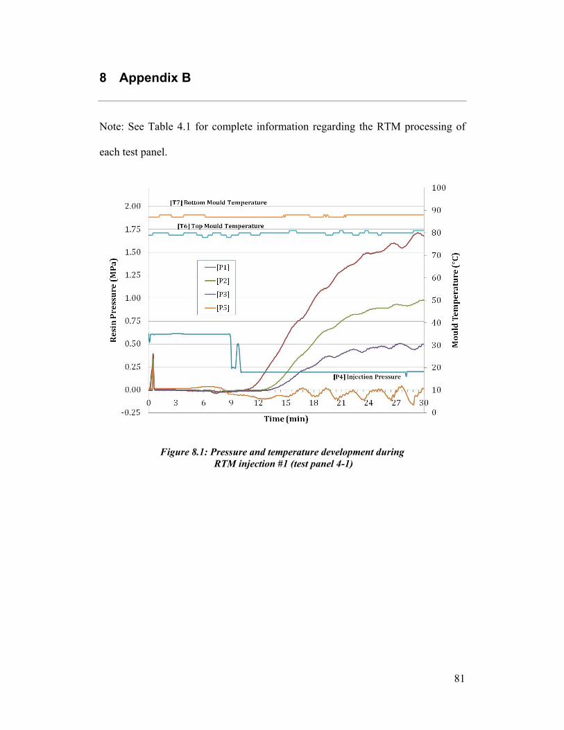
81
8 Appendix B
Note: See Table 4.1 for complete information regarding the RTM processing of
each test panel.
Figure 8.1: Pressure and temperature development during RTM injection #1 (test panel 4-1)
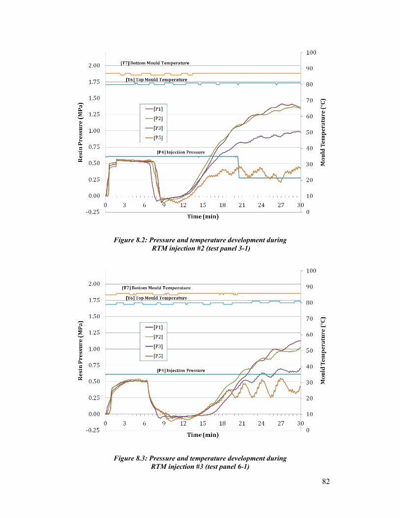
82
Figure 8.2: Pressure and temperature development during RTM injection #2 (test panel 3-1)
Figure 8.3: Pressure and temperature development during RTM injection #3 (test panel 6-1)
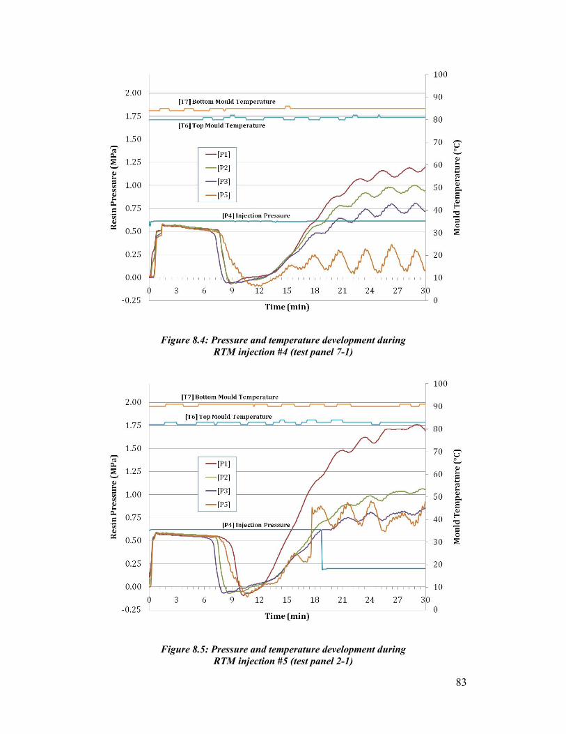
83
Figure 8.4: Pressure and temperature development during RTM injection #4 (test panel 7-1)
Figure 8.5: Pressure and temperature development during RTM injection #5 (test panel 2-1)
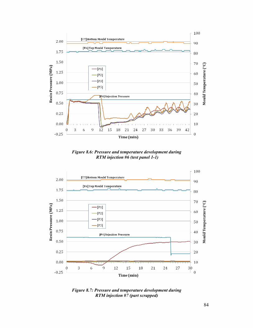
84
Figure 8.6: Pressure and temperature development during RTM injection #6 (test panel 1-1)
Figure 8.7: Pressure and temperature development during RTM injection #7 (part scrapped)
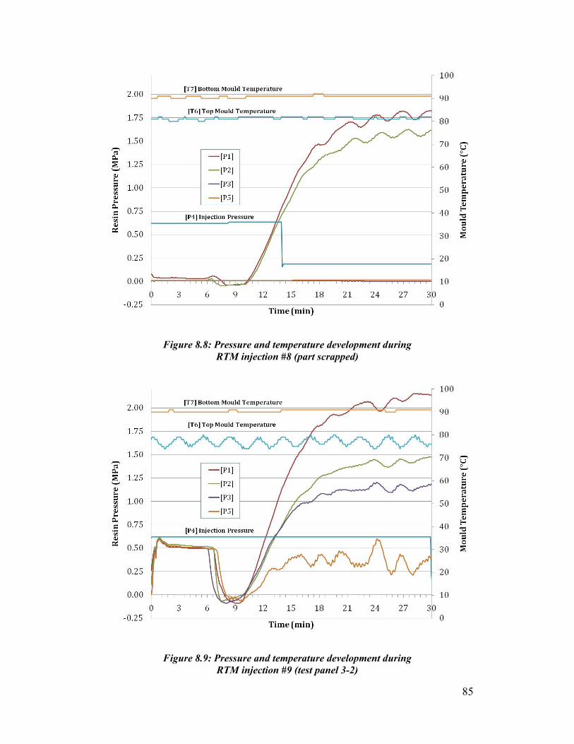
85
Figure 8.8: Pressure and temperature development during RTM injection #8 (part scrapped)
Figure 8.9: Pressure and temperature development during RTM injection #9 (test panel 3-2)
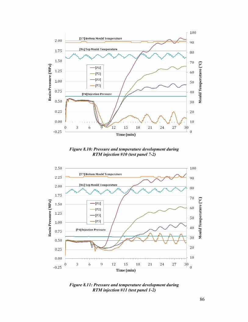
86
Figure 8.10: Pressure and temperature development during RTM injection #10 (test panel 7-2)
Figure 8.11: Pressure and temperature development during RTM injection #11 (test panel 1-2)
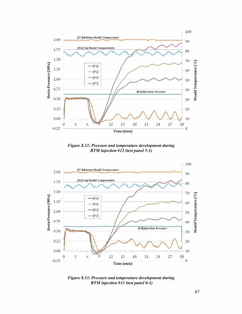
87
Figure 8.12: Pressure and temperature development during RTM injection #12 (test panel 5-1)
Figure 8.13: Pressure and temperature development during RTM injection #13 (test panel 8-1)
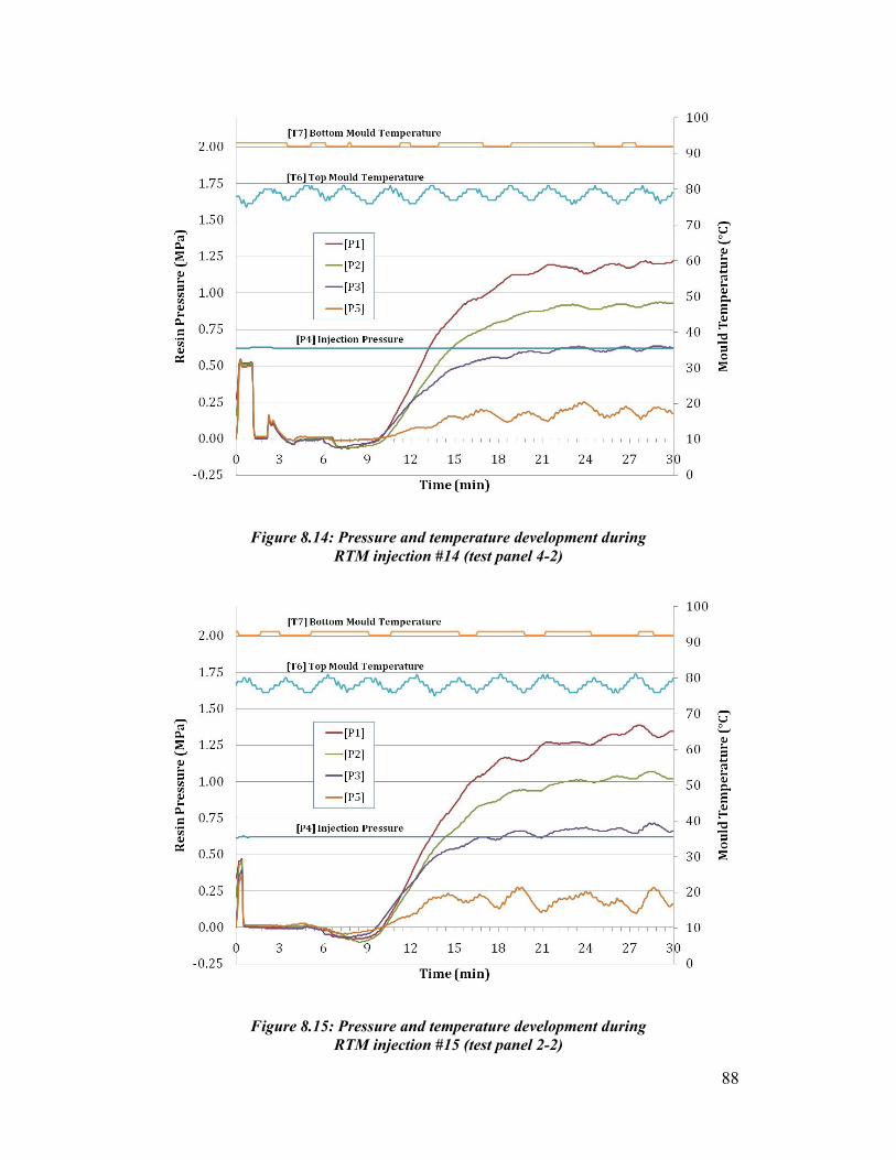
88
Figure 8.14: Pressure and temperature development during RTM injection #14 (test panel 4-2)
Figure 8.15: Pressure and temperature development during RTM injection #15 (test panel 2-2)

89
Figure 8.16: Pressure and temperature development during RTM injection #16 (test panel 6-2)
Figure 8.17: Pressure and temperature development during RTM injection #17 (test panel 8-2)
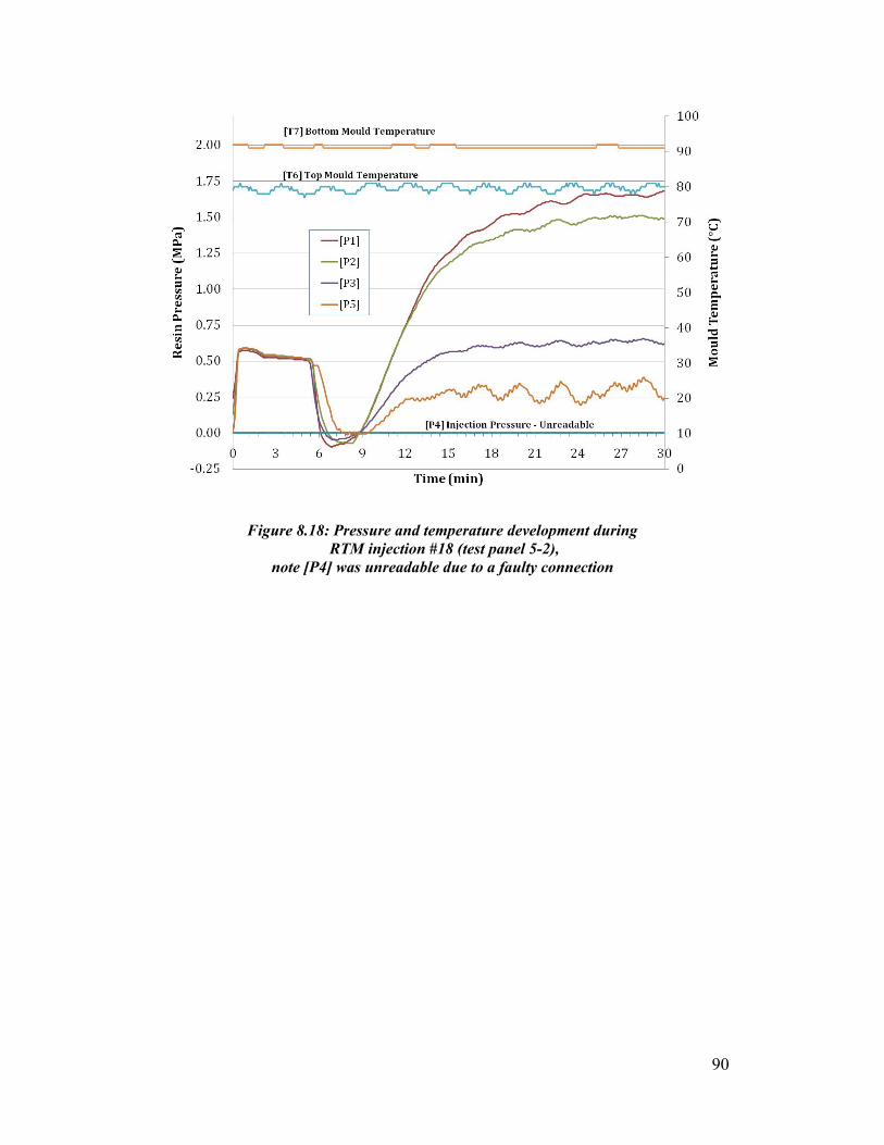
90
Figure 8.18: Pressure and temperature development during RTM injection #18 (test panel 5-2),
note [P4] was unreadable due to a faulty connection
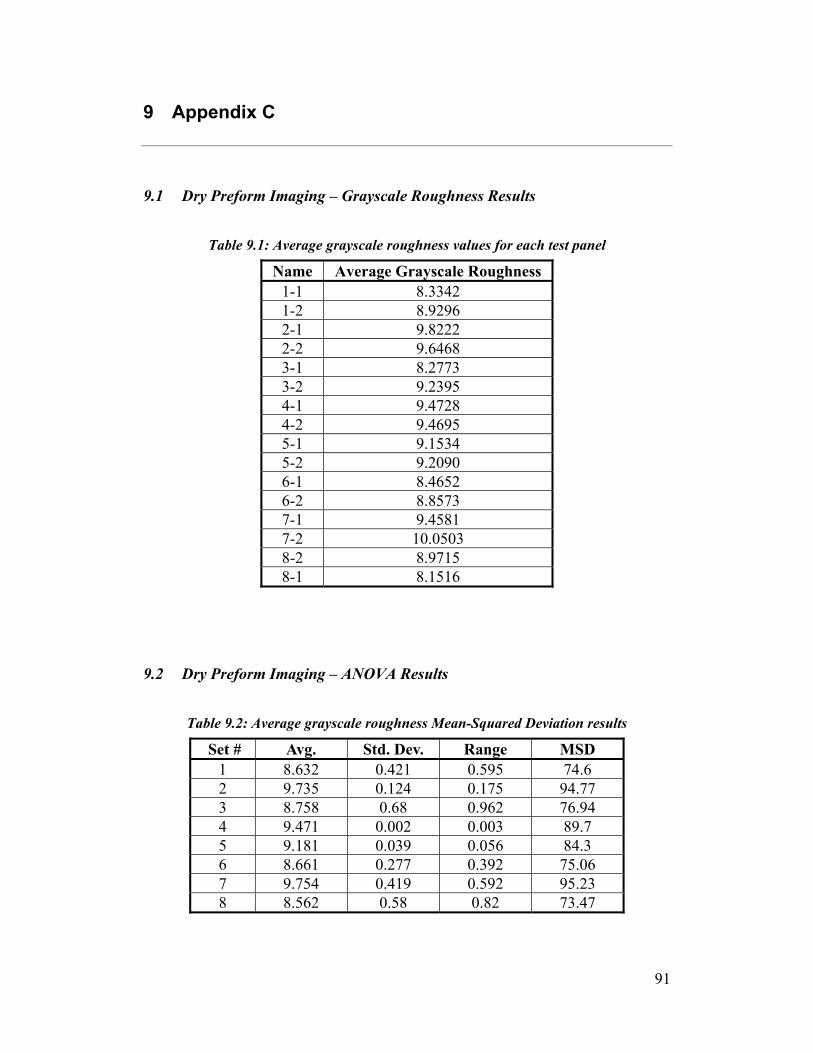
91
9 Appendix C
9.1 Dry Preform Imaging – Grayscale Roughness Results
Table 9.1: Average grayscale roughness values for each test panel
Name Average Grayscale Roughness 1-1 8.3342 1-2 8.9296 2-1 9.8222 2-2 9.6468 3-1 8.2773 3-2 9.2395 4-1 9.4728 4-2 9.4695 5-1 9.1534 5-2 9.2090 6-1 8.4652 6-2 8.8573 7-1 9.4581 7-2 10.0503 8-2 8.9715 8-1 8.1516
9.2 Dry Preform Imaging – ANOVA Results
Table 9.2: Average grayscale roughness Mean-Squared Deviation results
Set # Avg. Std. Dev. Range MSD 1 8.632 0.421 0.595 74.6 2 9.735 0.124 0.175 94.77 3 8.758 0.68 0.962 76.94 4 9.471 0.002 0.003 89.7 5 9.181 0.039 0.056 84.3 6 8.661 0.277 0.392 75.06 7 9.754 0.419 0.592 95.23 8 8.562 0.58 0.82 73.47
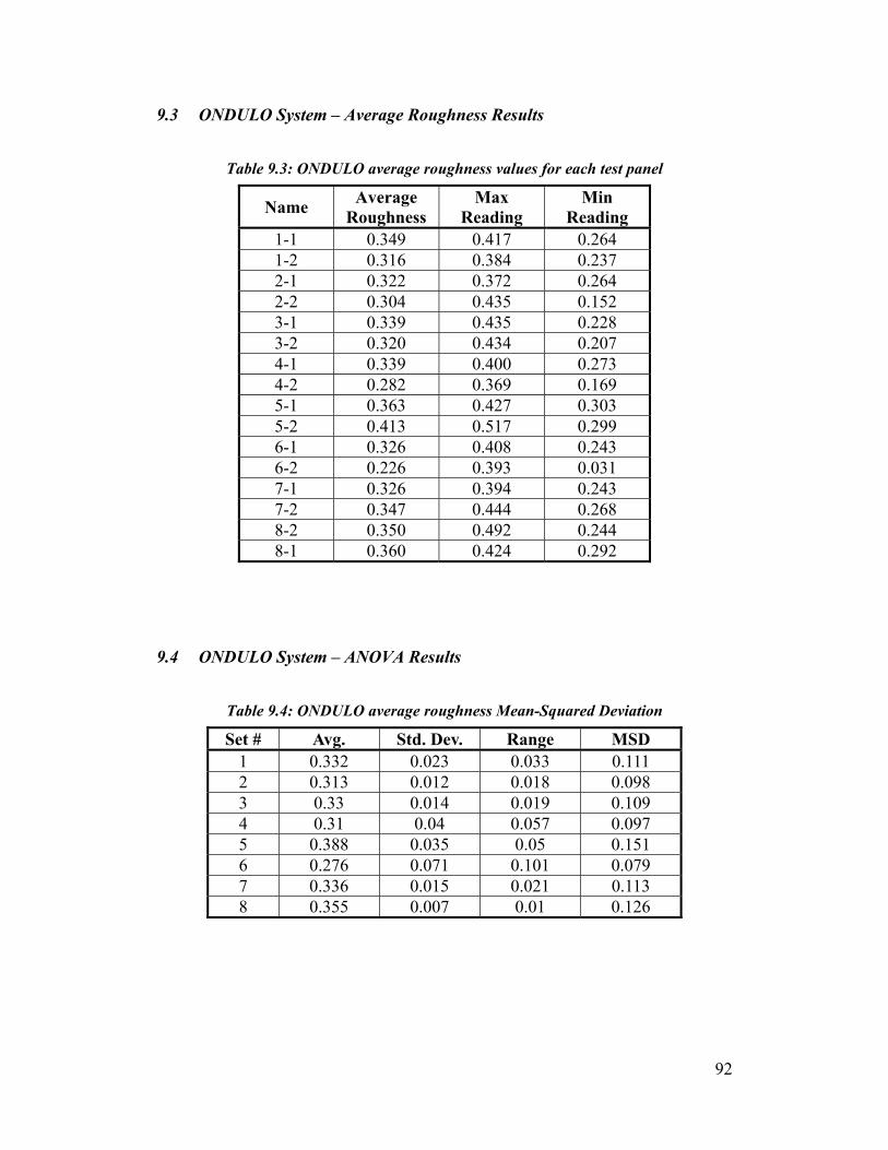
92
9.3 ONDULO System – Average Roughness Results
Table 9.3: ONDULO average roughness values for each test panel
Name Average Roughness
Max Reading
Min Reading
1-1 0.349 0.417 0.264 1-2 0.316 0.384 0.237 2-1 0.322 0.372 0.264 2-2 0.304 0.435 0.152 3-1 0.339 0.435 0.228 3-2 0.320 0.434 0.207 4-1 0.339 0.400 0.273 4-2 0.282 0.369 0.169 5-1 0.363 0.427 0.303 5-2 0.413 0.517 0.299 6-1 0.326 0.408 0.243 6-2 0.226 0.393 0.031 7-1 0.326 0.394 0.243 7-2 0.347 0.444 0.268 8-2 0.350 0.492 0.244 8-1 0.360 0.424 0.292
9.4 ONDULO System – ANOVA Results
Table 9.4: ONDULO average roughness Mean-Squared Deviation
Set # Avg. Std. Dev. Range MSD 1 0.332 0.023 0.033 0.111 2 0.313 0.012 0.018 0.098 3 0.33 0.014 0.019 0.109 4 0.31 0.04 0.057 0.097 5 0.388 0.035 0.05 0.151 6 0.276 0.071 0.101 0.079 7 0.336 0.015 0.021 0.113 8 0.355 0.007 0.01 0.126