Effect of pH on Coatings Used to Protect Aluminum ......Effect of pH on Coatings Used to Protect...

Effect of pH on Coatings Used to Protect Aluminum

Beverage Cans

by

Iwona Lazur

A thesis submitted to the Faculty of Graduate and Postdoctoral

Affairs in partial fulfilment of the requirements for the degree of

Master of Applied Science

in

Materials Engineering

Carleton University

Ottawa, Ontario

© 2014

Iwona Lazur

ii

Abstract

This study investigated the performance of epoxy-free coatings used to protect aluminum

beverage cans from corrosion in acidic solutions. Electrochemical Impedance

Spectroscopy and cyclic voltammetry tests were used to distinguish good and bad

coatings by monitoring the corrosion of the underlying aluminum. The goal of this work

was to understand how coatings protect the aluminum in spite of holes and holidays in

the coating. Bad coatings were made by introducing pinholes. Three scenarios were

found to hinder or stop corrosion: change from neutral to acidic pH, de-aeration using

carbon dioxide gas, and the formation of bubbles. This study concluded that the

formation of bubbles on the exposed surface of the aluminum, in concert with the

coating, protects the aluminum from corrosion in acidic solution.

iii

Acknowledgements

I would like to first thank my thesis supervisors, Professor Glenn McRae and Dr.

David McCracken. Their support, guidance, and patience throughout my research were

instrumental in me completing my work. I would also like to thank my colleague

Mohammad Ali for his help.

I would like to thank Yudie Yuan, John Hunter, and Ganesh Bhaskaran.

I would also like to thank my family and friends for their support and

encouragement throughout my graduate studies.

iv

Table of Contents

Abstract .............................................................................................................................. ii

Acknowledgements .......................................................................................................... iii

Table of Contents ............................................................................................................. iv

List of Tables ................................................................................................................... vii

List of Figures ................................................................................................................. viii

Chapter 1 Introduction ..................................................................................................1

1.1 Background .......................................................................................................... 1

1.2 Problem ................................................................................................................ 2

1.3 Thesis Objective and Scope ................................................................................. 3

1.4 Organization of Thesis ......................................................................................... 5

1.5 Methodology ........................................................................................................ 5

Chapter 2 Literature Review ........................................................................................6

2.1 Electrochemical Impedance Spectroscopy ........................................................... 6

2.1.1 Basis of Impedance ....................................................................................... 6

2.1.2 Circuit Elements............................................................................................ 9

2.1.3 Nyquist Plots ............................................................................................... 12

2.1.4 Bode Plots ................................................................................................... 15

2.2 Test Cell and Electrodes ..................................................................................... 16

2.3 Corrosion ............................................................................................................ 19

2.3.1 Aluminum ................................................................................................... 20

2.3.2 Polarization ................................................................................................. 25

2.3.3 Environmental Variables ............................................................................ 29

2.3.4 Corrosion of Aluminum .............................................................................. 30

v

2.4 Wetting ............................................................................................................... 35

2.5 Polymer Chemistry ............................................................................................. 36

2.6 Testing Methods ................................................................................................. 37

2.6.1 Conventional Methods ................................................................................ 38

2.6.2 EIS Methods used with Coatings ................................................................ 40

2.7 Previous Studies ................................................................................................. 45

2.7.1 Beverage Can Corrosion ............................................................................. 45

2.7.2 Coating Properties ....................................................................................... 53

Chapter 3 Equipment and Experimental Setup ........................................................55

3.1 Introduction ........................................................................................................ 55

3.2 Aluminum Samples ............................................................................................ 55

3.3 Test Cell ............................................................................................................. 55

3.4 Reference Electrode, pH Reader, and De-aerating Setup .................................. 56

3.5 Data Acquisition Equipment .............................................................................. 57

3.6 Solutions ............................................................................................................. 58

3.7 Experimental Procedure ..................................................................................... 59

Chapter 4 Results of Experiments ..............................................................................64

4.1 Effect of pH on Corrosion .................................................................................. 64

4.1.1 Sample A ..................................................................................................... 64

4.1.2 Sample B ..................................................................................................... 85

4.2 Effect of De-Aeration of Solution Using Carbon Dioxide ................................. 93

4.2.1 Sample C ..................................................................................................... 93

4.2.2 Sample D ..................................................................................................... 97

4.3 Formation of Bubbles ......................................................................................... 99

vi

4.3.1 Sample E ................................................................................................... 100

4.3.2 Sample F ................................................................................................... 102

Chapter 5 Discussion of Results ................................................................................109

5.1 Summary: Effect of pH on Corrosion .............................................................. 109

5.2 Summary: Effect of De-aerating Using Carbon Dioxide ................................. 110

5.3 Summary: Formation of Bubbles ..................................................................... 110

5.4 Interpretations and Explanations ...................................................................... 110

Chapter 6 Concluding Remarks and Recommendations .......................................119

References .......................................................................................................................122

vii

List of Tables

Table 2-1: Circuit Elements [10] ........................................................................................ 9

viii

List of Figures

Figure 1-1: Schematic of a Coating Containing Linked Pores ........................................... 4

Figure 2-1: Current Response to a Sinusoidal Voltage Input at a Given Frequency [10] .. 8

Figure 2-2: A Resistor and Capacitor in Series (R|C Circuit) [11] ................................... 11

Figure 2-3: A Resistor and Capacitor in Parallel (R||C Circuit) [10] ................................ 12

Figure 2-4: Nyquist Plot for a R||C Circuit Showing Impedance Vector and Other Major

Features [11] ..................................................................................................................... 13

Figure 2-5: Nyquist Plot for an Ideal Coating [11] ........................................................... 15

Figure 2-6: Bode Plot of an Ideal Coating [11] ................................................................ 16

Figure 2-7: Schematic of a Typical Test Cell ................................................................... 17

Figure 2-8: 2 Electrode Setup (Left) and 3 Electrode Setup (Right) [19] ........................ 18

Figure 2-9: Pourbaix Diagram for Aluminum and Water System at 25°C [25] ............... 22

Figure 2-10: Evans Diagram for Active-Passive Metal [28] ............................................ 27

Figure 2-11: Polarization Curve Displaying Common Features....................................... 28

Figure 2-12: Corrosion Pit in Metal M Displaying Autocatalytic Process in Aerated NaCl

[22] .................................................................................................................................... 31

Figure 2-13: Polarization Curve Showing Pit Formation [31] .......................................... 33

Figure 2-14: Pit Propagation of Aluminum [25]............................................................... 34

Figure 2-15: Hydrophilic and Hydrophobic Contact Angles [36] .................................... 36

Figure 2-16: Randles Circuit [21] ..................................................................................... 40

Figure 2-17: Circuit Model for a Failed Coating [21] ...................................................... 42

Figure 2-18: Bode Plot for Intact Coating (Curve 1) and Failed Coating (Curve 2). Curve

1: Rsol = 5 Ω, Rp = 1·108Ω, C = 5·10

-11 F. Curve 2: Rsol = 5 Ω, Rpol = 1·10

7Ω, Cc = 5·10

-

11 F, Rp = 1·10

6Ω, Cd1 = 5·10

-8 F, A = 1 cm

2. [21] ........................................................... 43

ix

Figure 2-19: Bode Plots and Nyquist Plots of Typical Intact, Damaged, Damaged (CPE)

and Diffusion (Warburg) Coatings [47] ............................................................................ 44

Figure 2-20: Typical impedance Bode plot showing the low and high break-point

frequencies [48] ................................................................................................................ 46

Figure 2-21: Impedance Spectra for Coated Aluminum Alloy at Times Before and After

Intentional Defect [49] ...................................................................................................... 49

Figure 2-22: Comparison of the Bode Phase Plots for Coated and Uncoated Aluminum

Samples in Acidic Chloride Solution [49] ........................................................................ 50

Figure 2-23: Proposed Equivalent Circuit Model for Coated Aluminum in Chloride

Solution [49] ..................................................................................................................... 51

Figure 3-1: Horizontal Test Cell ....................................................................................... 56

Figure 3-2: A Good Blank Sample Containing No Measurable Pre-existing Defects ..... 61

Figure 3-3: A Poor Blank Sample Containing Pre-existing Defects ................................ 62

Figure 4-1: EIS Bode Plot Results in Distilled Water (pH 7) for Sample A Containing a

Pinhole (Gamry)................................................................................................................ 66

Figure 4-2: EIS Nyquist Plot Results in Distilled Water (pH 7) for Sample A Containing

a Pinhole (Gamry) ............................................................................................................. 67

Figure 4-3: Cyclic Voltammetry Results for Sample A in Distilled Water (pH 7).

Potential Range: -2 V to +2 V (Gamry) ............................................................................ 68

Figure 4-4: EIS Bode Plot Results in HCl (pH 0) for Sample A Containing a Pinhole

(Gamry) ............................................................................................................................. 69

Figure 4-5: EIS Nyquist Plot Results in HCl (pH 0) for Sample A Containing a Pinhole

(Gamry) ............................................................................................................................. 70

x

Figure 4-6: Cyclic Voltammetry Results for Sample A in HCl (pH 0). Potential Range: -

2 V to +2 V (Gamry) ......................................................................................................... 71

Figure 4-7: Cyclic Voltammetry Results for Sample A in HCl (pH 3.8). Potential Range:

-2 V to +2 V (Gamry) ....................................................................................................... 72

Figure 4-8: Second Cyclic Voltammetry Results for Sample A in HCl (pH 3.8). Potential

Range: -2 V to +2 V (Gamry) ........................................................................................... 73

Figure 4-9: Second Cyclic Voltammetry Results for Sample A in HCl (pH 0). Potential

Range: -2 V to +2 V (Gamry) ........................................................................................... 74

Figure 4-10: Third Cyclic Voltammetry Results for Sample A in HCl (pH 3.8). Potential

Range: -2 V to +2 V (Gamry) ........................................................................................... 75

Figure 4-11: Second Cyclic Voltammetry Results for Sample A in Distilled Water (pH 7).

Potential Range: -2 V to +2 V (Gamry) ............................................................................ 76

Figure 4-12: EIS Bode Plot Results in Distilled Water (pH 7) for Sample A Containing a

Pinhole. Performed 9 days after Initial Tests (Solartron) ................................................ 77

Figure 4-13: EIS Nyquist Plot Results in Distilled Water (pH 7) for Sample A Containing

a Pinhole. Performed 9 days after Initial Tests (Solartron) ............................................. 78


Performed 9 days after Initial Tests. Potential Range: -2 V to +2 V (Solartron) ............ 79

Figure 4-15: Cyclic Voltammetry Test Results for Sample A in Distilled Water (pH 7).

Performed 9 days after Initial Tests. Potential Range: -3 V to +3 (Solartron) ................ 80

Figure 4-16: EIS Bode Plot Results in HCl (pH 0) for Sample A Containing a Pinhole.

Performed 9 days after Initial Tests (Solartron) ............................................................... 81

xi

Figure 4-17: EIS Nyquist Plot Results in HCl (pH 0) for Sample A Containing a Pinhole.


Figure 4-18: EIS Bode Plot Results in HCl (pH 5.3) for Sample A Containing a Pinhole.


Figure 4-19: EIS Bode Plot Results in HCl (pH 2) for Sample A Containing a Pinhole,

Left Overnight in Distilled Water (pH 7) (Solartron) ....................................................... 84

Figure 4-20: Microscopic Image of Sample A Pinhole (Post-experiments, 200x

Magnification)................................................................................................................... 85

Figure 4-21: Microscopic Image of Sample B Pinhole (Pre-experiments, 200x

Magnification)................................................................................................................... 86

Figure 4-22: EIS Bode Plot Results in Distilled Water (pH 7) for Sample B Containing a

Pinhole (Solartron) ............................................................................................................ 87

Figure 4-23: EIS Bode Plot Results in HCl (pH 1) for Sample B Containing a Pinhole

(Solartron) ......................................................................................................................... 88

Figure 4-24: Two EIS Bode Plot Results for Sample B Containing a Pinhole in

(Solartron): Distilled Water (pH 7) (Left) and HCl (pH 1) (Right) .................................. 89

Figure 4-25: Third EIS Bode Plot Results in HCl (pH 1) for Sample B Containing a


Figure 4-26: Microscopic Image of Sample B Pinhole (Post-experiments, 200x

Magnification)................................................................................................................... 92

Figure 4-27: Microscopic Image of Sample B Damage (Post-experiment, 200x

Magnification)................................................................................................................... 92

xii

Figure 4-28: EIS Bode Plot Results in Distilled Water (pH 7) for Sample C Containing a


Figure 4-29: EIS Nyquist Plot Results in Distilled Water (pH 7) for Sample C Containing

a Pinhole (Solartron) ......................................................................................................... 95

Figure 4-30: EIS Bode Plot Results for Sample C Containing a Pinhole in De-aerated

Distilled Water (pH 7) (Solartron) .................................................................................... 96

Figure 4-31: EIS Nyquist Plot Results in De-aerated Distilled Water (pH 7) for Sample C

Containing a Pinhole (Solartron) ...................................................................................... 97

Figure 4-32: EIS Bode Plot Results for Sample D Containing a Pinhole in KCl (pH 4)

(Solartron) ......................................................................................................................... 98

Figure 4-33: EIS Bode Plot Results for Sample D Containing a Pinhole in De-aerated

KCl (pH 4) (Solartron) ...................................................................................................... 99

Figure 4-34: EIS Bode Plot Results for Sample E Containing a Pinhole in KCl (pH 4)

(Solartron) ....................................................................................................................... 101

Figure 4-35: Cyclic Voltammetry Results for Sample E in KCl (pH 4). Potential Range: -

2.5 V to +3 V (Solartron) ................................................................................................ 102

Figure 4-36: Cyclic Voltammetry Results for Sample F in De-aerated Distilled Water (pH

7). Potential Range: -2.5 V to +3 V (Solartron) ............................................................. 103

Figure 4-37: EIS Bode Plot Results for Sample F Containing a Pinhole in De-aerated

Distilled Water (pH 7) (Solartron) .................................................................................. 104

Figure 4-38: Second Cyclic Voltammetry Results for Sample F in De-aerated Distilled

Water (pH 7). Potential Range: -2.5 V to +3 V (Solartron) ........................................... 105

xiii

Figure 4-39: Second EIS Bode Plot Results for Sample F Containing a Pinhole in De-

aerated Distilled Water (pH 7) (Solartron) ..................................................................... 106

Figure 4-40: Third Cyclic Voltammetry Results for Sample F in De-aerated Distilled

Water (pH 7). Potential Range: -2.5 V to +3 V (Solartron) ........................................... 107

Figure 4-41: Cyclic Voltammetry Results from Figure 4-36 and Figure 4-40 Overlaid to

Emphasize the Similarities .............................................................................................. 108

Figure 5-1: Three Major Steps of Bubble Formation in Liquid on a Heated Metal Surface:

Nucleation, Growth, and Bubble Release [56] ............................................................... 115

Figure 5-2: Proposed Bubble Formation Process for a Coating-Aluminum System with a

Pinhole in Strongly Acidic Solution ............................................................................... 117

1

Chapter 1 Introduction

1.1 Background

Aluminum used to make beverage cans is coated inside and outside with a resin to

protect from corrosion. Beverage cans made with aluminum alloy are favoured due to

them being lightweight and their ability to be recycled [1]. They are also easier to

transport and store compared to beverage containers made of glass. Aluminum beverage

cans have good anti-corrosion properties in neutral solutions, however, in the presence of

acidic solutions aluminum corrodes [1]. For instance, Coke™ has a pH 2.38 and Diet

Coke™ has a pH 2.92 [2]. Epoxy resins are commonly used as coatings to protect

aluminum from corrosion [3]. A resin starts as a liquid which changes to a solid with a

hard finish when set [3]. Two types of resins exist: natural, also called oleoresins, and

synthetic. Traditionally synthetic epoxy resins are used to coat beverage cans. These

resins contain bisphenol A (BPA), which is introduced into the coating during production

[4]. There is a concern that BPA may leach into the liquid contained inside beverage

cans.

BPA is included in the Domestic Substances List (DSL), which identifies

substances used in Canadian commerce [5]. This list is updated by the Chemicals

Management Plan (CMP), managed by Environment Canada and Health Canada [5] [6].

CMP assesses chemicals to determine if they are harmful to human health. If a chemical

is found to be harmful, the CMP takes action to protect consumers [6]. The CMP

identified BPA as a chemical of concern [4].

2

1.2 Problem

Health Canada has decided to focus on BPA intake in infants because baby

formula is often stored in cans coated with resins containing BPA or in plastic bottles that

contain BPA [4]. The decision was based on the possibility of formula being the only

nutrition an infant receives. Health Canada reviewed reports, submitted by the Plastic

Industry (SPI), on the effects BPA had on human health. Toxicology studies submitted

before 1979 were also reviewed. It was found that BPA may affect the reproduction

system in high doses (139 times higher than the probable intake for the general public

and 9.5 times higher for infants). This was due to it behaving similarly to estrogen and

possibly acting as an endocrine disruptor [4]. Reports, with dates ranging from 2004 to

2007, describe the effects of high doses of BPA on rats and mice. These reports showed

that very high doses were capable of causing side effects such as behavioural changes

(mice became more anxious), and an increase in certain hormones in rats during early

puberty (testosterone in males and estradiol in females). These very high doses, however,

ranged from over 1 thousand to 11 million times the probable intake for the general

public, and 76 to 76 thousand times the probable intake for infants [4].

Health Canada determined that at current levels of BPA consumption for the

general public and infants, BPA does not pose a health risk, because of the extreme doses

required to see side effects in rats and mice [4]. Japan, the United States, the European

Union, and other health agencies published the same conclusion. Health Canada,

however, stated that further research must be conducted on the effects of BPA, especially

in infants, to address several drawbacks found in reports from 2004 to 2007. Some of

these drawbacks include certain tests using only single doses of BPA, not being able to

3

reproduce results in other laboratories, and lack of consistency. In the meantime, Health

Canada has recommended that exposure to BPA from food packaging should be lowered

[4]. The US Food and Drug Administration (US FDA) has also stated that they would

support the exposure of BPA being lowered or eliminated in can coatings [3]. Industries

have started to look for alternatives to epoxy resins that would not contain BPA, but

would be able to protect the food, maintain the same quality, and not cause health risks

greater than that of BPA [3] [4].

In spite of the unrealistically high doses required to produce side effects, the

perception of the general population is that BPA is bad for human health. Thus,

removing BPA is a priority for the food and beverage industry.

1.3 Thesis Objective and Scope

The objective of this thesis was to answer the following question:

How can beverage can coatings work in low pH solutions despite the presence of

holidays?

We want to understand how the coatings work to aid in the development of BPA-free

coatings because BPA is a safety concern for the public.

The scope of this thesis was to conduct short-term tests on beverage can material

using Electrochemical Impedance Spectroscopy (EIS) and cyclic voltammetry. Tests

were conducted in solutions that simulated soft drinks, and in solutions with pH of 0 and

7 to understand the effect of aluminum oxide formation. Acidity of commercial soft

drinks varies greatly; the pH of beverages are typically between pH 2.3 to pH 4 [2] [7].

For instance, Coke™ is pH 2.38, and Barq‟s Root Beer is pH 4 [2] [7].

4

Beverage can coatings are thought to provide a barrier between the liquid and the

aluminum, however, these coatings have pores, flaws, defects and holidays1. In addition,

aluminum is not protected by an adherent oxide layer at low pH because aluminum oxide

is not stable (Section 2.3.1). Hence, if the coating is not a perfect barrier, and low pH

solution is able to reach the underlying aluminum, then the can should fail rapidly from

corrosion. Even though these coatings have holidays, the cans can last for years.

Initially, it was believed that the coatings would perform better in neutral solutions than

in acidic solutions because a protective plug of stable aluminum oxide would fill the

pathways that exist between holidays and pores that lead to the aluminum surface. Figure

1-1 shows the pores connecting to create pathways to the aluminum surface.

Figure 1-1: Schematic of a Coating Containing Linked Pores

Contrary to this expectation, previous experiments have shown that beverage can

coatings performed better in acidic pH than neutral [8]. The goal of this work is to

understand how a coating with holidays can perform better in acidic solution than neutral,

1 Holidays are defects in a coating; they are small holes in a coating where the base metal is unprotected

[23] [57]

5

and the implications for new BPA-free coatings. The work in this thesis is a continuation

of the work presented in the thesis by M. Ali [8].

1.4 Organization of Thesis

This thesis contains 5 chapters. Chapter 1 discusses background information on

beverage cans, as well as the problem definition and objective of this thesis. Chapter 2

introduces the reader to the concept of EIS, as well as a literature review of the latest

research related to this thesis. The experimental setup and the equipment used are

described in Chapter 3. Chapter 4 covers the test results and Chapter 5 the discussion of

these results. Chapter 6 presents the conclusions and recommendations for future

experiments.

1.5 Methodology

The research in this thesis was conducted using EIS and cyclic voltammetry. A

pinhole through the coating was created in aluminum beverage can samples to represent a

holiday. The pinhole was then tested to examine the behaviour of the coating when it

was exposed to three different effects: change of pH, de-aeration of the solution, and

bubble formation. The methodology is discussed in greater depth in Chapter 3.

6

Chapter 2 Literature Review

2.1 Electrochemical Impedance Spectroscopy

An EIS experiment uses a sinusoidal voltage or current perturbation [9]. The

perturbation is applied over a range of frequencies, which makes it possible to measure

and analyze the electrochemical response over a wide frequency range. EIS is widely

used due to the large amount of data and information that it provides. It is used in many

fields including: corrosion, fuel cell development, paint characterization, and battery

development [9]. EIS was created in the 1880s by Oliver Heaviside [10]. Soon after A.

E. Kennelly and C. P. Steinmetz generated complex number equations and vector

diagrams that made it possible to better present EIS data [10].

2.1.1 Basis of Impedance

In an electrical circuit, impedance, Z, is related to voltage and current by Ohm‟s

Law:

2-1

where V(t) and I(t) are the time dependent voltage and current, respectively [10]. In the

special case where there is no time dependence, the impedance is known as resistance

and is given the symbol R. In this case Ohm‟s Law becomes:

2-2

Voltage (or potential) is measured in volts [V], current is measured in amperes [A], and

resistance and impedance are measured in ohms [Ω] [10].

7

Impedance includes information on the phase difference that occurs between

voltage and current. Impedance can be separated into a real portion, which is the in-

phase component associated with energy loss, and an imaginary portion which is the 90°

out-of-phase component associated with storing electrical energy [10].

In this thesis, sinusoidal voltages are applied across coatings and the resulting

time-dependent currents are measured [11]. The voltage can be expressed as [10]:

2-3

where VA is the amplitude [V], f is the frequency [Hz], t is the time [s], and ω is the radial

frequency [rad/s]. In this thesis, for the voltage amplitudes used, the current response

was linear, with the same shape and frequency, but with a phase shift between 0 to –π/2

rads (0° to -90°). The equation for the current response is [10]:

2-4

where IA is the current amplitude [A] and θ is the shift in phase [rads]. Figure 2-1 shows

a plot of the current response to a sinusoidal voltage input. Depending on the circuit, the

current will either lead or lag the voltage [10]. In Figure 2-1 the current is leading the

voltage by the phase shift θ.

8

Figure 2-1: Current Response to a Sinusoidal Voltage Input at a Given Frequency

[10]

The voltage function and current function can be expressed as a complex relationship

[10]:

2-5

2-6

where j is equal to √-1. Using equations 2-1, 2-5 and 2-6, the impedance equation can be

written as [10]:

2-7

where the last relationship is determined using Euler‟s equation. Equation 2-7 can be

separated into real and imaginary components as follows [10]:

9

2-8

2-9

2-10

Impedance can also be expressed equivalently by using its magnitude [10]:

| | √ 2-11

and a phase angle [10]:

2-12

In this thesis, impedance will be described in terms of its real and imaginary components

and/or its magnitude and phase angle.

2.1.2 Circuit Elements

The electrical responses of coatings used to protect beverage cans can also be

described in terms of passive linear circuit elements. Table 2-1 lists the typical circuit

elements that are used when modelling EIS results.

Table 2-1: Circuit Elements [10]

Component Equivalent Element Impedance

Resistor R [ohm] R

Capacitor C [F, or ohm-1

s] 1/jωC

Inductor L [H, or ohm s] jωL

Constant Phase Element Q [ohm-1

sα] 1/Q(jω)

α

10

Table 2-1 shows that the impedance of a resistor is independent of frequency [10]. There

is only a real component to the impedance of a resistor. Hence, the voltage and current

are always in phase with each other.

A capacitor is another passive electric circuit element [11] [12]. A typical

configuration of a capacitor consists of a material, known as a dielectric, sandwiched on

two sides by conducting plates. A capacitor can store energy. For a capacitor, the

impedance decreases as the frequency increases [10]. A capacitor only has an imaginary

impedance component. Unlike a resistor, the current of a capacitor is shifted -90° to its

voltage. The capacitance can be calculated using the following equation:

2-13

where C is the capacitance [F], A is the area of the electrodes, d is the distance between

the electrodes, εo is the constant electrical permittivity of a vacuum (8.85·10-14

F/cm) and

ε is the relative permittivity of the material between the electrodes (which reflects the

ability of the material that is being analyzed to store electrical energy) [10]. In this thesis,

the dielectric material will be the coating, which is attached on one side to the aluminium

beverage can alloy. The alloy acts like one of the plates of a capacitor. The other side of

the dielectric coating is exposed to solution containing electrolytes, which behaves like

the second plate of the capacitor.

An inductor is another passive electric circuit element [10]. While it also has only

an imaginary impedance like a capacitor, its impedance increases as frequency increases

and its current is shifted +90°compared to its voltage [10].

A fourth passive circuit element used in modelling EIS spectra is the constant

phase element (CPE). The equation for the impedance of a CPE contains a parameter α,

11

which can be used when the dielectric is fractal or as a fitting parameter [13] [14]. As an

example, the double-layer capacitor, discussed in Section 2.2 , is described as a CPE [10].

There exist special cases for values of α. When α is equal to 1, then the CPE coefficient,

Q, is equal to C, and the CPE impedance is equivalent to the impedance of a pure

capacitor. If α equals 0 the CPE impedance becomes the impedance of an ideal resistor,

where R is equal to 1/Q. If α equals -1 the CPE impedance becomes equivalent to the

impedance of an inductor. There also exists another special case when α is equal to 0.5,

where the CPE impedance becomes the Warburg impedance for homogenous semi-

infinite diffusion [10].

Passive circuit elements can be combined to create equivalent circuits which

model electrochemical systems. Two simple circuits are shown below. A resistor and

capacitor in series, known as a R|C circuit, is shown in Figure 2-2.

Figure 2-2: A Resistor and Capacitor in Series (R|C Circuit) [11]

The impedance of a R|C circuit can be calculated as [11]:

2-14

When a resistor and a capacitor are in parallel with each other a R||C circuit is formed,

shown in Figure 2-3.

12

Figure 2-3: A Resistor and Capacitor in Parallel (R||C Circuit) [10]

The impedance of a R||C circuit can be calculated as [10]:

2-15

(

)

2-16

2.1.3 Nyquist Plots

A Nyquist plot, also called a complex plane impedance diagram, is created when

the negative imaginary portion of the impedance equation (Equation 2-10) is plotted on

the vertical axis and the real portion is plotted on the horizontal axis [10] [15]. Each

point on the Nyquist plot is the impedance at one frequency. Figure 2-4 shows a Nyquist

plot for a typical R||C circuit. The impedance can be expressed as a vector on the Nyquist

plot [11] [15]. This vector has a length equal to the magnitude of the impedance

(Equation 2-11). The phase angle can also be expressed as the angle between the

impedance magnitude vector and the horizontal axis (Equation 2-12).

13

Figure 2-4: Nyquist Plot for a R||C Circuit Showing Impedance Vector and Other

Major Features [11]

In Figure 2-4 the frequencies are implicit in the plot. Following the curve from

right to left the frequency increases, as shown by the arrow. This does not occur for all

circuits or at all AC frequencies but is usually the case when impedance increases as

frequency decreases [10] [15].

An advantage of a Nyquist plot is that if a dielectric has multiple components with

different time constants, it will be readily seen in the plot [10] [12]. A plot with a single

semi-circle will have one time constant. For each additional semi-circle there exists

another time constant. In general, the time constant can be expressed as:

2-17

where the R and C depend on the components. The magnitude of the resistor is the

diameter of the semi-circle in a Nyquist plot. This thought to be due to the impedance

being purely capacitive at the highest frequency but purely resistive at the lowest

frequency. As the frequency approaches zero, the impedance approaches the value of the

14

resistor. Examples of processes with single time constants are charge-transfer and

activation-energy-controlled mechanisms [10].

A Nyquist plot does not always have a single full semi-circle with the center of

the semi-circle on the real axis [13]. There are several reasons for why the center of the

semi-circle may be located in the complex plane. One scenario is where the arc does not

pass through the origin. This may be caused by R∞ having a value greater than zero

and/or the plot containing more arcs at higher frequencies. Another scenario is when the

material-electrode system contains distributed elements. This will cause the time

constant to no longer equal a single value, but instead be distributed continuously or

discretely around a mean time constant. The width of the distribution of a time constant

is related to the angle by which a semi-circle arc has been depressed below the real axis.

Another reason for distorted semi-circle is the presence of other mean time constants that

have values within two orders of magnitude or less of the semi-circle being analyzed.

Overlapping semi-circles may be observed if this occurs [13].

The inductive loop is another feature of a Nyquist plot [10] [16] [17] [18]. It

appears as a loop with a positive imaginary component at lower frequencies2. Strictly

speaking these are pseudo-inductances that occur because of chemistry on the surface.

For instance, the appearance of an inductive loop has been associated with weakening of

the protective aluminum oxide layer by the dissolution of the aluminum alloy [10] [16]

[17] [18].

The shape of a Nyquist plot can reveal if a coating is functioning well or if it has

failed [10]. An ideal perfect coating would appear as a vertical line in the Nyquist plot,

similar to the one shown in Figure 2-5 [10].

2 Can also occur at higher frequencies due to mutual inductance [56].

15

Figure 2-5: Nyquist Plot for an Ideal Coating [11]

The corrosion process involves transfer of electrons. If the coating performs well as an

electrical barrier, it will also perform well as a corrosion barrier.

2.1.4 Bode Plots

Another common way to represent EIS data is to use a Bode plot, in which the

frequency dependence is shown explicitly [10] [15]. In the Bode plot, the phase angle

and the logarithm of the impedance magnitude are plotted against the logarithm of the

frequency. Figure 2-6 shows a Bode plot for an ideal coating. The impedance of an ideal

coating behaves like a capacitor; it is very high at low frequencies (i.e., greater than 1010

Ω at 0.1 Hz for the coatings used in this work), the impedance plot is a straight line with

a slope of -1, and the phase angle is -90° [11]3. In this thesis, positive phase angles and

impedances with a positive slope are indications of a bad coating; when these features are

present the underlying aluminum is corroding. This interpretation is supported by the

3 The rise in phase angle at high frequencies is due to inductance of the cables. See footnote 2.

16

observation that when cathodic protection is applied, positive phase angles and

impedances with positive slopes disappear [8].

Figure 2-6: Bode Plot of an Ideal Coating [11]

2.2 Test Cell and Electrodes

An EIS experimental setup consists of an electrolyte, a working electrode, a

counter electrode, and a reference electrode [19]. The working electrode is where the

corrosion reactions occur in the electrochemical system. In this study, the working

electrodes are the coated aluminum samples. The counter electrode is usually an inert

material, like graphite, that is used to complete the current path in the test cell, and to act

as a current source and current sink. A reference electrode provides an offset potential

relative to a standard [19].

The three common experimental setups for studying coatings use 2 or 3 electrodes

[19]. Generally, electrodes are solids immersed in electrolyte [19]. Figure 2-7 shows a

schematic of a typical test cell. The reference and counter electrodes are inserted into the

electrolyte [20]. The working electrode is held flush against one side of the cell. The

17

right end of the cell contains a through hole that allow electrolyte to make contact with

the working electrode [20].

Figure 2-7: Schematic of a Typical Test Cell

In a typical experiment electrical connections are made between the measuring

instrument and electrodes using 4 leads: working, counter, working-sense, and reference

[19]. Figure 2-8 shows schematics for 2 and 3 electrode setups. The working and

counter leads carry the current, while the working-sense and reference leads measure the

potential. A reference electrode is capable of maintaining a constant potential. Ideally it

experiences only minimal current flow so that its voltage is unaffected by the current

flowing in the cell. When the currents are low in the test cell (less than or equal to μA)

the counter electrode can be used as the reference electrode since the potential drops are

miniscule; this is a 2 electrode setup [19]. In this type of setup the working and working-

sense electrodes are connected together, and the counter and reference electrodes are

18

connected together. In this case the inert material of the counter electrode is acting as a

reference point for the measured potential, as well as the counter electrode [19].

Figure 2-8: 2 Electrode Setup (Left) and 3 Electrode Setup (Right) [19]

A 3 electrode cell also has the working and working sense electrodes connected together,

but has separate counter and reference electrodes [19]. The potential of the counter

electrode can change without affecting the potential between the working electrode and

reference electrode. Using an independent reference electrode in this way allows

accurate measurement of the potential of the working electrode [19].

An electrode and an electrolyte form an electrical double layer at their interface

[11]. When ions from the electrolyte attach themselves to the electrode surface the

double layer is formed. The double layer causes the charged electrode to be separated

from the charged ions in the electrolyte. This separation, which is usually on the order of

0.1 nanometers (10-10

m), causes a double layer capacitance to form. The double layer

capacitor is influenced by many factors including: temperature, oxide layers, electrode

roughness, and electrode potential [11]. The double layer capacitor creates an energy

barrier between the metal and the electrolyte [21].

19

2.3 Corrosion

Corrosion is defined as the reaction, either chemical or electrochemical, of a

material with its environment which causes the material to deteriorate [22]. Corrosion

characteristically occurs in electrolyte solutions. An electrolyte may be alkaline, neutral

or acidic. When a metal is immersed in an electrolyte and begins to corrode there is a

transfer of electrons between two different areas on the metal. An area of a metal that is

giving up electrons is called an anode. An area where the electrons are being absorbed is

called a cathode. An electrical circuit forms since there exists a potential difference

between the anode and cathode. Electrons flow through the metal from the anode to the

cathode and ions diffuse through the solution, in particular positively charged ions and

solutes, e.g., H+ and O2, flow from the electrolyte solution to the cathode, where they are

reduced by electrons [23].

An anodic reaction occurs when electrons are produced. It also called an

oxidation [22]. The general anodic reaction is:

2-18

The anodic reaction for aluminum is [24]:

2-19

A cathodic reaction, or a reduction, occurs when electrons are consumed. Several

cathodic reactions can occur during metallic corrosion [22]. More than one cathodic

reaction and one anodic reaction can occur simultaneously. When a metal is exposed to

an acidic solution, hydrogen reduction is the cathodic reaction. The hydrogen reduction

reaction equation is:

20

2-20

Hydrogen gas is produced when hydrogen ions react with the electrons produced by the

anodic reaction.

Oxygen reduction is another cathodic reaction. It can occur in a mildly acidic

solution in the presence of air. If the solution is exposed to air the following reaction

may occur [22]:

2-21

In neutral or basic solutions the cathodic reaction is also called an oxygen reduction

reaction. The oxygen reduction equation for basic or neutral solutions is as follows:

2-22

During corrosion, both cathodic and anodic reactions must occur simultaneously. They

must also occur at the same rate to conserve charge. There must be equal production and

consumption of electrons [22].

2.3.1 Aluminum

A thin protective corrosion product film forms on the surface of most metals and

alloys [25]. The thin film is a result of the metal or alloy reacting with its environment.

Without the thin film on its surface a metal would return to its thermodynamically stable

condition. Some metals and alloys produce a film that creates a corrosion resistant

surface. These films are called passive films and are the cause of passivity of a metal or

alloy. [25]

21

Passivity is difficult to define but can be considered as a metal or alloy losing its

chemical reactivity when placed in certain environments [22]. A metal or alloy that has

become passive can be thought of as becoming inert and acting as a noble metal [22].

The ability of aluminum to resist corrosion is caused by its capacity to passivate

under certain conditions [25]. The passivity of aluminum is caused by the formation of a

barrier oxide layer that protects the underlying aluminum from particular corrosive

environments. The formation of a protective oxide film in solutions of different pH can

be predicted approximately by using a Pourbaix diagram, which can be used to determine

at which thermodynamic conditions the oxide layer may form. Figure 2-9 gives the

Pourbaix diagram for aluminum in 25 °C water [25].

22

Figure 2-9: Pourbaix Diagram for Aluminum and Water System at 25°C [25]

The diagram contains three types of regions: an immunity region, a passivation

region, and two corrosion regions [26]. The immunity region, where the metal is immune

to corrosion, is bounded above by lines 1, 2, and 3. Line 1 corresponds to the equilibrium

reaction [24]:

23

2-23

Line 2 corresponds to the equilibrium reaction:

2-24

Line 3 corresponds to the equilibrium reaction:

2-25

In the passivation region, the oxide that forms depends on the environmental conditions

[24] [25]. At lower temperatures, aluminum trihydroxide, Al(OH)3, tends to form. At

higher temperatures, boehmite, Al2O3·H2O, tends to form. Hydrargilite, Al2O3·3H2O,

may form if aluminum hydroxide is aged. At very high temperatures, above

approximately 230 °C, a protective oxide no longer forms. The pH at which the oxide is

considered most stable is approximately 5, shown as line c [24] [25].

There are two corrosion regions in Figure 2-9, at high and low pH. Soluble Al3+

ions form at low pH values using equation 2-23. The soluble ions are in equilibrium with

the insoluble oxide shown by the vertical concentration lines on the left of the Pourbaix

diagram:

2-26

At high pH values, the soluble AlO2- ions are in equilibrium with the insoluble oxide

shown by the vertical lines on the right of the Pourbaix diagram:

2-27

24

Lines a and b in Figure 2-9 give the thermodynamic stability of water. These

limits are for water at 1 atmosphere and at 298 K. For the area below line a, water

becomes unstable due to the formation of hydrogen gas, which corresponds to the

following half reaction:

2-28

In the area above line b, water is unstable due to the formation of oxygen gas. Oxygen

gas formation corresponds to the following half reaction:

2-29

Between lines a and b water is stable relative to oxygen and hydrogen gas.

It is important to define the ionic activity that will be used to determine if

significant corrosion is occurring. An allowable amount of metal dissolution must be

decided upon to determine if there is corrosion. A solubility of 10-6

g atoms of soluble

ion per litre is customarily used as a threshold for the metal to be immune to corrosion.

The horizontal and vertical lines labelled 0 to -6 in Figure 2-9 are marked with the

logarithm of the activity and are used to determine the concentration.

Using this potential versus pH diagram, aluminum is passivated between

approximately pH 4 and 9 where stable aluminum oxide can form. The passivity of

aluminum is also influenced by the temperature of the aqueous solution, the type of oxide

that develops, and the assumption that there is a low dissolution of aluminum. Multiple

types of oxides show very little solubility at approximately pH 5 [25].

When placed in water or in atmospheres that are at ambient temperature the oxide

layer that develops to protect the aluminum is amorphous and has a thickness of a few

25

nanometers. However, when the temperature is increased, the thickness of the protective

oxide that is formed is also higher [25].

Using Figure 2-9 it can be seen that aluminum will corrode in alkaline and acidic

solutions due to the fact that no protective oxide forms in these solutions. When it

corrodes in alkaline solutions aluminum forms AlO2- ions. In acidic solutions Al

3+ ions

form. There are cases where the oxide layer is insoluble in solution or where it is stable

due to the oxidizing characteristics of a solution; acetic acid and sodium disilicate are two

examples. Due to the possibility of several different ions that can be present depending

on the environment, and due to the large influence ions have on the corrosion of

aluminum, there is no general relationship between corrosion rate and pH [25].

2.3.2 Polarization

A polarization curve, also known as an Evans diagram, is useful since it

demonstrates the kinetics of corrosion and not just the thermodynamic condition given by

the Pourbaix diagram [25]. The curve can be presented with potential (V) on the vertical

axis and the current density (I) on the horizontal axis, or vice versa [26]. The current

density is usually graphed on a logarithmic scale and with units of A/cm2 or A/mm

2

depending on the sample size. The current is a direct measure of the corrosion rate at that

particular voltage [26].

The two main polarization test procedures are galvanostatic and potentiodynamic

[26]. In the galvanostatic procedure, current is controlled by the instrument while the

potential is recorded. Using the potentiodynamic procedure, the potential is controlled

while the current is measured [26].

26

During a potentiodynamic polarization test the voltage is first increased in the

anodic direction, which is known as a forward scan [25]. After reaching a pre-set

voltage, the voltage is decreased in the cathodic direction, which is known as a reverse

scan. A cyclic voltammetry test is a type of potentiodynamic test where there can be one

or several forward and reverse scans. The corrosion potential is the potential at which the

anodic current, also called the corrosion current, and cathodic currents are equal [27].

The corrosion potential is usually the voltage selected as the starting point of a test [25].

A hysteresis loop is a common feature [25]. It occurs when the curve does not

follow the same path during the reverse scan as it did during the forward scan. A

hysteresis is created when there is a difference in current density between the two scans

at the same potential. A change in the chemical condition at the surface is responsible for

this feature. This may be passivation or the formation of permanent pits, which have the

opposite effects [25].

If the current density is greater on the reverse scan than on the forward scan, then

the corrosion rate has increased [25]. This can be symptomatic of localized corrosion,

such as pitting, that was induced during the forward scan. This clockwise loop is called a

positive hysteresis. A counter clockwise loop negative hysteresis occurs when the

current density is lower during the reverse scan than it was during the forward scan at the

same potential. This implies that re-passivation is occurring more readily than during the

forward scan. It can indicate that the sample is resistant to localized corrosion. Figure

2-10 shows the forward scan of an active-passive metal [25].

27

Figure 2-10: Evans Diagram for Active-Passive Metal [28]

An increase in metal corrosion rate is responsible for the increase in current

density above the corrosion potential [25]. At a maximum in current density, known as

the critical current, a high corrosion rate is observed. The potential at the critical current

is known as the passivation potential. Between the corrosion potential and the

passivation potential the metal is in an active state. The passivation potential is the

beginning of a transition between the active and the passive state, when a passive oxide

film begins to form on the surface of the metal, limiting the corrosion current. Since the

system is entering a passive state, the current density decreases. The passive current is a

constant current and is no longer dependent on the potential. At this time the rate of

formation and the rate of dissolution of the oxide are equal, resulting in a dynamic

28

equilibrium. The current density can once again increase if the oxide film that formed

during passivation breaks down. The break down can be caused by weak points within

the film, and often marks the start of pitting, in which case the potential at which this

occurs is called the pitting potential. Figure 2-11 shows some of the major features that

occur on a potentiodynamic polarization curve [25].

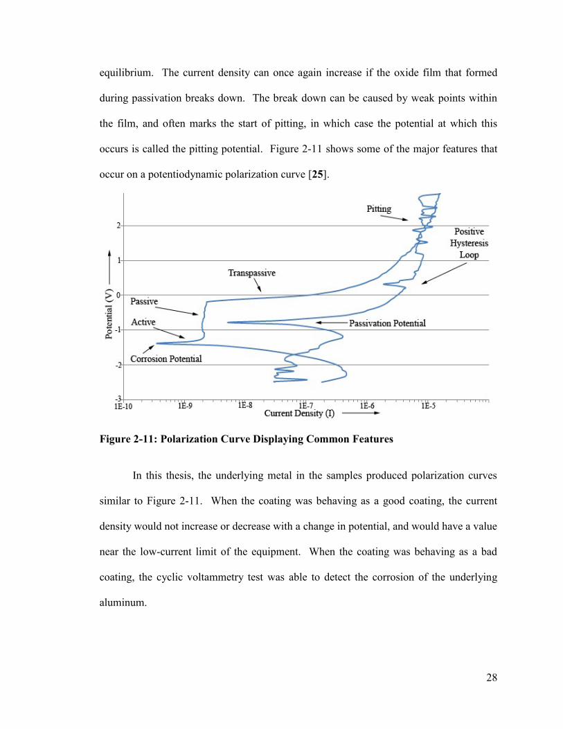
Figure 2-11: Polarization Curve Displaying Common Features

In this thesis, the underlying metal in the samples produced polarization curves

similar to Figure 2-11. When the coating was behaving as a good coating, the current

density would not increase or decrease with a change in potential, and would have a value

near the low-current limit of the equipment. When the coating was behaving as a bad

coating, the cyclic voltammetry test was able to detect the corrosion of the underlying

aluminum.

29

2.3.3 Environmental Variables

The presence of oxygen in a solution has an influence on the corrosion of

aluminum [25]. In a de-aerated solution, the corrosion of aluminum can be very slow.

When there is O2 present, however, corrosion occurs much faster. As the concentration

of dissolved oxygen in solution is increased, the corrosion rate also increases since

oxygen encourages attack. In particular this can be observed in acidic solutions [25].

Chloride ions have been suggested to hinder the motion of oxygen vacancies located in

the oxide [29]. Hydrogen and nitrogen gases do not influence the rate of corrosion [25].

Hydrogen sulphide and carbon dioxide have been observed to minimally slow down the

corrosion rate. This occurs even when their concentrations are high.

The concentration and nature of an acid affects the corrosion rate of aluminum

[25]. At room temperature a dilute sulphuric acid solution with a concentration

approximately 40% to 95% causes aluminum to corrode rapidly. If the concentration is

reduced to approximately 10% then the speed of the attack on the aluminum is greatly

reduced. A reduction in the corrosion rate also occurs at very high concentrations. A

dilute solution of phosphoric acid, with a concentration of less than 1%, does cause

corrosion in aluminum by etching the surface. When raised to an intermediate

concentration, the phosphoric acid no longer etches the surface of the aluminum but

instead attacks it more severely. Above approximately 0.1% concentration hydrobromic,

hydrofluoric and hydrochloric solutions cause aluminum to corrode [25].

The concentration of an alkaline solution also affects the corrosion of aluminum

[25]. Above 0.01% concentration sodium hydroxide and potassium hydroxide solutions

are highly corrosive to aluminum. Nearly neutral solutions, pH ranging from

30

approximately 5 to 8.5, of inorganic salts cause very little, or even a negligible amount of

corrosion at room temperature. If inorganic salts at this pH range do cause corrosion to

occur in aluminum it is usually highly localized in the form of pitting [25].

2.3.4 Corrosion of Aluminum

Pitting is a localized form of corrosion that causes a loss of metal [23]. It can be a

deep hole in a metal with a small opening on the surface. Pitting corrosion is difficult to

detect. As corrosion progresses the depth of the pit can increase significantly while the

opening increases very little. Frequently the opening may be covered in corrosion

product making it even more difficult to detect. It is also difficult to detect since pitting

does not cause a decrease in thickness of the metal or a large loss in weight. If a pit is

allowed to continue to grow it may eventually penetrate the thickness of the material and

may cause the component to fail [23].

The reaction within a corrosion pit is an anodic reaction that is a unique

autocatalytic process [22]. An autocatalytic process within the pit means that the

corrosion process that occurs does not only stimulate corrosion to continue but also

empowers the pit to keep growing. Figure 2-12 shows the autocatalytic process that

occurs within a corrosion pit in a metal. In this figure the metal is exposed to aerated

sodium chloride [22].

31

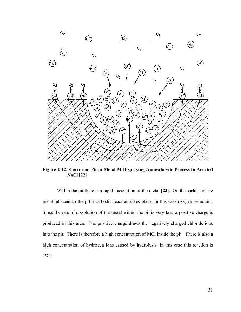
Figure 2-12: Corrosion Pit in Metal M Displaying Autocatalytic Process in Aerated

NaCl [22]

Within the pit there is a rapid dissolution of the metal [22]. On the surface of the

metal adjacent to the pit a cathodic reaction takes place, in this case oxygen reduction.

Since the rate of dissolution of the metal within the pit is very fast, a positive charge is

produced in this area. The positive charge draws the negatively charged chloride ions

into the pit. There is therefore a high concentration of MCl inside the pit. There is also a

high concentration of hydrogen ions caused by hydrolysis. In this case this reaction is

[22]:

32

2-30

The high concentrations of hydrogen ions and chloride ions accelerate the dissolution of

metal and cause the pit to grow [22].

There are four major stages of pitting [30]. The first stage includes processes that

occur at the boundary between the passive film and the solution. The second stage

includes the processes that occur within the passive film. At this stage no visible

microscopic changes have occurred. During the third stage metastable pits initiate and

grow. They grow for a short amount of time and stay below the critical pitting potential.

The metastable pits are small. The pits then repassivate. The time it takes for a

metastable pit to grow and repassivate can be only a few seconds. At the fourth stage the

pits experience stable growth. This occurs above a potential called the critical pitting

potential. Figure 2-13 shows a sample polarization curve which shows the formation of

pits [30].

33

Figure 2-13: Polarization Curve Showing Pit Formation [31]

Ecp is the critical pitting potential in this figure. The figure shows the metastable pits

forming below the critical pitting potential. When the metastable pits form, the current

oscillates. It increases when the pits form and grow [30]. After a short amount of time

the current decreases due to the pits repassivating. Figure 2-13 shows how this behaviour

appears as a zigzag pattern on a polarization curve. Metastable pits occur most often at

potentials close to the critical pitting potential. The amount of metastable pits on pure

aluminum can increase for two reasons when in contact with chloride ions. One

condition that causes metastable pits is an increase in anodic potential with a constant

34

concentration of chloride ions. Metastable pits can also occur when there is a constant

potential but the concentration of chloride ions is increased [30].

During the propagation stage of a pit in aluminum, aluminum within the pit is

dissolved into Al3+

ions [23]. Outside the pit or at the mouth of the pit a cathodic

reaction occurs. The cathodic reaction causes the reduction of H+ or oxygen ions. The

cathodic reaction may destroy the protective oxide layer locally. This reaction often

causes hydrogen liberation. The pH of the solution within the pit is lowered due to the

hydrolysis of water by Al3+

ions and the production of protons. A corrosion product

made of Al(OH)3 or Al2O3 forms at the mouth of the pit and may eventually block the pit

[23] [32]. Figure 2-14 shows the pitting process of aluminum.

Figure 2-14: Pit Propagation of Aluminum [25]

Models that simulate pit initiation exist. An unverified electrode kinetic model

for pit initiation has been developed by McCafferty [33]. This model uses the charge on

the oxide surface, as well as the pH of zero charge parameter. The model also takes into

account the penetration of chloride ions into the oxide film using oxygen vacancies, the

35

absorption of chloride ions on the oxide surface, and pit initiation at the metal/oxide

interface caused by the dissolution of the underlying substrate.

2.4 Wetting

It is important to understand the wetting behaviour of thin polymer films,

especially when the polymer is used as a coating [34]. The stability of the film is affected

by wetting and dewetting. The field of biophysics has studied “smart” surfaces which are

polymers that respond to a change in properties. These properties include a change in

pH, ion concentration, or temperature.

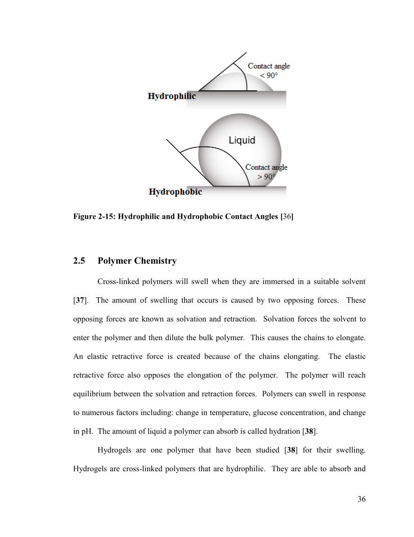
Wetting is the adhesion of a fluid to a solid surface [35]. Wettability is the

tendency of the fluids to adhere to, or wet, the surface of a solid. The fluid can be water,

oil, air, or any other liquid. A surface that is wettable is called hydrophilic or water-wet.

A surface that is non-wettable is called hydrophobic or oil-wet. The contact angle

between a drop of water and a horizontal surface of a solid object can be observed to

determine if a polymer is hydrophilic or hydrophobic. When the drop of water is spread

out, with a contact angle of less than 90°, the polymer is hydrophilic. An infinitely

hydrophilic polymer would theoretically have a contact angle of 0°. When the contact

angle is greater than 90° the polymer is hydrophobic, with an infinitely hydrophobic

polymer having a contact angle of 180°. If the contact angle is exactly 90° then the

polymer is naturally wet [35]. Figure 2-15 shows two droplets of water on a solid

surface; one droplet is considered to be hydrophilic and the other one is considered to be

hydrophobic.

36

Figure 2-15: Hydrophilic and Hydrophobic Contact Angles [36]

2.5 Polymer Chemistry

Cross-linked polymers will swell when they are immersed in a suitable solvent

[37]. The amount of swelling that occurs is caused by two opposing forces. These

opposing forces are known as solvation and retraction. Solvation forces the solvent to

enter the polymer and then dilute the bulk polymer. This causes the chains to elongate.

An elastic retractive force is created because of the chains elongating. The elastic

retractive force also opposes the elongation of the polymer. The polymer will reach

equilibrium between the solvation and retraction forces. Polymers can swell in response

to numerous factors including: change in temperature, glucose concentration, and change

in pH. The amount of liquid a polymer can absorb is called hydration [38].

Hydrogels are one polymer that have been studied [38] for their swelling.

Hydrogels are cross-linked polymers that are hydrophilic. They are able to absorb and

37

maintain water in their structure without being dissolved. The hydration of hydrogels is

driven and caused by their hydrophilic nature. The cross-linked network structure limits

the amount of hydration of a polymer. Non-ionic swelling of a polymer decreases as the

degree of cross-linking increases [37]. The swelling of polymer particles in a hydrogel

membrane has also been studied. The membrane must be optically transparent, inert to

the solvents used, permeable, and allow for the polymer particle to swell in a uniform

manner. Turbidimetry is used to measure the swelling of particles since there is a change

in their refractive index when they swell.

In the 1970s, polymer swelling was tested by placing the polymer in dyed solvent

and then examining its cross section using a microscope [39]. The sample was weighed

before and after being placed in the solvent, as well as recording its dimensions before

and after. The measurement of small changes in the surface of the polymer caused by a

weak solvent and the measurement of thin films are not reliable because of the very small

changes that occur in the polymer. Polymer swelling has been measured using: quartz

crystal micro balance, ellipsometry, electrical conductivity, laser interferometry, surface

plasmon resonance spectroscopy, and combinations of micro-mechanical cantilever

sensors and surface plasmon resonance spectroscopy.

2.6 Testing Methods

This section will discuss the corrosion testing methods related to beverage cans.

38

2.6.1 Conventional Methods

Corrosion tests in sealed cabinets have been used to determine the corrosion

performance of coatings since the 1900s [40]. They can be used to accelerate corrosion

of coatings and reduce the time it takes to obtain results. A cabinet corrosion test consists

of placing a sample within a cabinet containing a corrosive environment. The corrosive

environment depends on the sample and may include the use of one or more of the

following: salt fog, hot and cold temperatures, corrosive gas, humidity and exposure to

ultraviolet light [40].

The salt fog test, also called a salt spray test, is the most used common cabinet

corrosion test [40]. There exist American Society for Testing and Materials (ASTM)

standards for this test which dictate the setup and procedure [40]. Typically, a 5%

sodium chloride solution is formed into a fine aerosol fog and a steady 35 °C temperature

is kept within the cabinet, however, some industries use a 20% sodium chloride solution

and higher temperatures. A typical salt fog test can last for months or years. During the

test, the samples are often periodically inspected. The salt fog test is useful as a process

control test; for instance, time-to-failure in the salt fog can be used to determine the

relative benefits of changing process/manufacturing variables. However, standalone salt

fog tests do not necessarily correlate well with in-service performance because of the

different chemical reactions and circumstances that occur in service [40].

There exist variations to the salt fog test [40]. Tests on decorative chromium

plating on steel, lasting for a few hundred hours, use a 5% sodium chloride salt fog spray

that has been acidified with acetic acid to pH 3.2. Exfoliation testing on some aluminum

alloys is done using a 5% sodium chloride solution that has been acidified using acetic

39

acid to pH 2.9, and at 49 °C. The test consists of 0.75 hours of spray, 2 hours of dry air

purge, and then 3.25 hours of soaking at a high humidity, making the test duration 6

hours. There exist other variations including a salt/SO2 spray fog test, acidified synthetic

sea water fog test, cyclic salt fog and UV exposure test, and dilute electrolyte cyclic fog

and dry test. Salt fog tests are also used in conjunction with other tests. For instance, a

filiform test consists of a salt spray followed by an exposure to 70% to 90% relative

humidity. Filiform corrosion, which appears as threadlike strands, forms under finishes.

Filiform corrosion can occur in powder-clear-coated aluminum and only forms when the

relative humidity is between 70% and 95% [40].

Electrochemical methods, using alternating currents (AC) and direct current (DC),

are also used to test coatings [40]. Anodized aluminum can be tested using the Ford

anodized aluminum corrosion test, also known as FACT. A cylindrical glass cell is

clamped onto the surface of the sample and filled with a 5% sodium chloride solution

containing cupric chloride, which is acidified with acetic acid. The sample is

cathodically polarized by applying a DC voltage between the sample and an electrode

immersed in the solution for 3 minutes. The resistance of the coating can decrease over

this time, leading to a larger current. This test is no longer an ASTM standard due to

certain aluminum alloys failing the test but performing well in service. FACT is also

known as cathodic breakdown test when the DC polarization is -1.6 V versus a saturated

calomel electrode [40].

Electrochemical noise methods (ENM) are non-destructive tests that appraise the

susceptibility of a material to localized corrosion. In an electrochemical system, potential

and current fluctuations/noise occur [41]. ENM record these fluctuations as a function of

40

time. No artificial noise or fluctuations are imposed on the system when using ENM

[42]. ENM can produce results that provide information on corrosion rates and

mechanisms. While the instruments used to collect data for ENM are inexpensive and

simple to use, ENM is not widely used because the data can be difficult to interpret and

associate with in service performance. There exist three main approaches to interpret

ENM data. These are the statistical, spectral, and chaos theory-based methods [42].

2.6.2 EIS Methods used with Coatings

Equivalent electrical circuits are a popular method used by researchers and

authors to analyze measured EIS data [43] [44]. This method assumes a relationship

between electrical circuit components and physical features in the EIS data. The Randles

circuit is a common model that is used to represent a metal coated with a polymer [21]

(Figure 2-16).

Figure 2-16: Randles Circuit [21]

Rsol is the solution resistance, CC is the coating capacitance, and Rp is the pore or

flaw/parallel resistance, which represents all the conductive paths which exist through the

coating [43] [45]. The impedance of the Randles circuit is given by [21]:

41

2-31

At high frequencies the impedance of the Randles circuit is equal to the solution

resistance, because the impedance of the capacitor is smaller than the solution resistance

(the impedance of a capacitor varies as one over the frequency (Table 2-1)) [10]. At mid

frequencies, the capacitive component dominates, and at low frequencies the pore/parallel

resistance is the least resistive path.

An intact coating demonstrates a capacitive behaviour and high impedance at low

frequencies. In this study, the impedance ranged from 107

Ω to 1010

Ω at frequencies

lower than 10 Hz. Depending on the data acquisition equipment used, measurements of

the impedance at the higher end of the range were more-or-less unreliable (Section 3.5 ).

As a coating degrades, the low-frequency impedance decreases. In this study, when the

impedance was lower than 107

Ω below 10 Hz, the coating was no longer protective.

Generally, a good coating does not contain conductive paths through pores and/or flaws,

and can be represented as a capacitor [43]. As the coating begins to fail, the pores and/or

flaws in the coating are filled with electrolyte solution, which create conductive paths

[43].

Figure 2-17 shows the coating model commonly used for a failed coating. In this

figure, Cd1 is the double layer capacitance and Rpol is the polarization resistance [21].

Polarization resistance represents the impedance of the electrode in the system having its

potential changed from its corrosion potential [46]. The change in the potential of the

electrode causes current flow, which is caused by electrochemical reactions at the surface

of the electrode. The magnitude of the current flow is controlled by the diffusion of

reactants moving away from and towards the electrode, and reaction kinetics [46].

42

Figure 2-17: Circuit Model for a Failed Coating [21]

Figure 2-18 shows a simulation of the Bode plot for a good/intact coating, Curve 1, and a

breached/failed coating, Curve 2. Curve 1 was modelled with a Randles circuit and

Curve 2 with the failed coating circuit model [21]. In this figure, Rp ranges from 106 Ω to

108

Ω. In this thesis, Rp for good/intact coatings was over 1010

Ω. The figure shows how

the shape of a Bode plot might change when the coating degrades [47].

43

Figure 2-18: Bode Plot for Intact Coating (Curve 1) and Failed Coating (Curve 2).

Curve 1: Rsol = 5 Ω, Rp = 1·108Ω, C = 5·10

-11 F. Curve 2: Rsol = 5 Ω, Rpol

= 1·107Ω, Cc = 5·10

-11 F, Rp = 1·10

6Ω, Cd1 = 5·10

-8 F, A = 1 cm

2. [21]

It is not always possible to use an ideal capacitor to model experimental data [47]. When

the coating is non-uniform, has a rough surface, or has an inhomogeneous distribution of

current, a constant-phase element (CPE) is used instead of a capacitor for the model in

44

Figure 2-17. The Warburg impedance is used when the corrosion rate is controlled by the

diffusion through electrolyte or the pores of the coating. An indication of Warburg

impedance is a 45° tail in the low frequency region in the Nyquist plot. Figure 2-19

shows simulations for the Bode plots and Nyquist plots for: an intact coating; a damaged

coating modeled with an ideal capacitor; a damaged coating modeled with a CPE; and a

damaged coating modeled with a Warburg impedance [47]. In this thesis, an ideal/intact

coating does not display the same behaviour as the simulation shown in Figure 2-19. An

ideal coating in this thesis shows the behaviour described in Section 2.1.3 and Section

2.1.4.

Figure 2-19: Bode Plots and Nyquist Plots of Typical Intact, Damaged, Damaged

(CPE) and Diffusion (Warburg) Coatings [47]

45

2.7 Previous Studies

This section will focus on previous studies on beverage can corrosion as well as

studies on coating properties.

2.7.1 Beverage Can Corrosion

The two year pack-test is an industry standard [48]. It requires the use of visual

examination, which causes this method to not always be reliable. To increase the speed

of testing, aggressive solutions like acidic solutions or an applied voltage have been used.

Using an acidic solution or an applied voltage during a two year pack-test causes the test

to no longer be food product specific. F.S. Bovard et al [48] conducted a test where food

cans underwent a two year pack-test. The food cans were then examined both visually

and with EIS. To evaluate the coatings quantitatively they reduced the impedance

spectrum to a single numerical performance indicator. They used three different methods

to find a numerical performance indicator. The three methods were: using low frequency

impedance [log(Z) at 0.04 Hz], using break-point frequency (θ = 45°), and percent ideal

behaviour [48].

The low frequency impedance method assumed a Randles equivalent circuit [48].

F.S. Bovard et al [48] found that the low frequency impedance, taken at 0.04 Hz, was

approximately equal to the sum of the charge transfer resistance, the solution resistance,

and the coating resistance. The low frequency impedance was also found to correspond

to the coating degradation that was visually observed, which appeared as blisters [48].

The break-point frequency method also assumed a Randles equivalent circuit

[48]. This method focused at the point where there is a change from capacitive to

resistive behaviour in the impedance response, at a phase angle of θ = 45°. This method

46

was used when the charge transfer resistance could not be determined because of too

much noise at the lower frequencies. A Randles circuit with two time constants can have

two break-point frequencies [48]. A Bode plot showing two break-point frequencies can

be seen in Figure 2-20.

Figure 2-20: Typical impedance Bode plot showing the low and high break-point

frequencies [48]

The high break-point frequency occurs when the impedance of the coating is

changing to the solution resistance (which can be negligible) plus the pore resistance

[48]. The low break-point frequency occurs when the impedance is changing to the

solution resistance, plus the pore resistance, plus the charge transfer resistance. The high

47

break-point frequency was the primary break-point frequency used when comparing data

in this study [48], however, it was not always measurable by the researchers. The low

break-point frequency was used when the high break-point frequency was not available

[48].

The percent ideal behaviour method reduced EIS data to a single numerical

performance indicator [48]. This method used the ratio of the area under a Bode

magnitude curve versus the area under an ideal capacitive curve. A coating is evaluated

depending on how close its curve is to the ideal capacitive curve; the closer this curve is

to the ideal capacitive curve, the better the coating is. This method gives it an advantage

over the other two methods as it uses the entire frequency spectrum [48].

The paper concluded that EIS can be used to inspect coatings when using food

product as the electrolyte [48]. All three methods correlated well with the traditional

visual inspection. It was found that the low frequency impedance method worked well

when there was no noise. It was also the easiest to use since the data was obtained

straight from the Bode plot. The break-point frequency method was not always accurate

since the high break-point frequency was not always measurable. Lastly, while the

percent ideal method used the whole frequency spectrum, the drawback found was that it

had to be calculated [48].

A two part study by Grandle and Taylor [49] [50] acknowledged that there is a

need to replace current beverage can coatings due to proposed changes in regulations

concerning volatile organic compounds, as well as a need to store more aggressive

materials inside polymer coated aluminum cans. The first part of the study focused on

finding an EIS parameter, which will be discussed, that is easy to obtain and can also be

48

used to evaluate the performance of coatings [49] [50]. The second part of the study took

the parameter that was found and evaluated samples of coatings.

Before an EIS parameter could be found, the authors first compared the

impedance responses of an uncoated aluminum alloy sample to the impedance response

of a coated aluminum alloy sample without any defects and a coated aluminum alloy

sample with a defect [49] [50], which can be seen in Figure 2-22. This made it possible

to determine the parts of the impedance spectrum related to the coating and the solution-

oxide-metal interface. Three different thicknesses of a proprietary epoxy-acrylic polymer

were used. The intentional defect was approximately 0.1 mm in diameter and was made

using a carbide scribe [49] [50].

Figure 2-21 shows the EIS results for a sample before and after a defect was made

[49] [50]. It was observed that prior to the defect the EIS response of the intact coating

was almost purely capacitive. After the defect was made the EIS response became more

complex, with more than one time constant becoming visible. The impedance also began

to decrease at the low frequency end of the spectrum [49] [50].

49

Figure 2-21: Impedance Spectra for Coated Aluminum Alloy at Times Before and

After Intentional Defect [49]

The sample used in Figure 2-21 was compared to an uncoated aluminum alloy

sample [49] [50]. It was determined that the phase angle peak that occurred at 96 hours

and 5 Hz was due to water and ion ingress into the defect, which caused reactions to

occur with the metal and/or oxide. By comparing the damaged coated sample, shown in

Figure 2-22, with the uncoated sample it was also determined that the second time

50

constant for the damaged coated sample occurred at the same frequency as the time

constant for the uncoated sample [49] [50].

Figure 2-22: Comparison of the Bode Phase Plots for Coated and Uncoated

Aluminum Samples in Acidic Chloride Solution [49]

The authors suggest that this time constant therefore contained information about

the reactions such as charge transfer occurring at the metal surface, and/or information

about the oxide [49] [50]. The high frequency time constant was believed to provide

information on the coating, including the overall coating capacitance. An increase in the

size of the defect, caused by new defects forming or the original defect increasing in size,

was thought to have caused the decrease in interfacial impedance that was observed after

96 hours [49] [50].

The study also included EIS results for coated and uncoated samples placed under

DC polarization [49] [50]. When the potential was in the transition region (Section 2.3.2)

51

the data was scattered at low frequencies. It was suggested that the scatter was caused by

the current fluctuating as metastable pits formed [49] [50].

Figure 2-23 shows a very complex proposed circuit model for a coated aluminum

sample in chloride solution [49] [50]. The change in coating capacitance with time was

used to study water content in the film, however, Brasher‟s equation assumes that the

change in coating capacitance was caused only by water permeating into the coating. It

also assumes that the distribution of water in the coating is uniform but random. Failure

due to the coating blistering or spot corrosion could not be predicted using the change in

coating capacitance [49] [50].

Figure 2-23: Proposed Equivalent Circuit Model for Coated Aluminum in Chloride

Solution [49]

Data was fitted to the model in Figure 2-23 and the coating capacitance values were

obtained [49] [50]. The coating capacitance was then plotted versus time. After five

52

months of exposure the coating capacitances of the samples increased approximately 5%

or less with time. The samples were not all failing, due to spot corrosion, at the same

rate. Only the sample with the intentional defect showed a large change in coating

capacitance which may have been caused by water ingress into the intentional defect. It

was determined that observing changes in coating capacitance cannot be used to predict

failure or as a parameter to measure performance [49] [50].

Pore resistance was also considered a possible parameter [49] [50]. It was

determined that, while short term observations of the pore resistance did well in

correlating to the changes observed after 5 months, it could not be used as a parameter in

a large test. This is due to the pore resistance requiring fitting to the circuit in Figure

2-23 which can be difficult and time consuming. The pore resistance decreased by orders

of magnitude when the coating was severely degraded and was impossible to obtain when

the pore resistance became low [49] [50].

The magnitude of the low frequency impedance, between 0.01 and 0.05 Hz, was

used as the parameter to evaluate the performance of coatings [49] [50]. This parameter

could be easily obtained from a Bode plot or a Nyquist plot. While it gave information

on how the coating was failing, it was also found to correlate with the performance of the

coating. The average low frequency impedance was plotted on a log scale versus time of

exposure in days. If the log average low frequency impedance remained the same the

coating was not considered degrading. The performances of different coatings were

ranked by comparing their log average low frequency impedance at specified exposure

times. A coating with a higher parameter magnitude at the same exposure time as other

coatings was considered to be performing better. The magnitude of the low frequency

53

impedance was found to reflect the change in defect area and the charge transfer response

[49] [50]. Gui and Kelly [51] went on to analyze the performance of corrosion

prevention compounds using the method described by Grandle and Taylor [49] [50].

They suggested that the double layer capacitance could also be used as a performance

parameter, where a lower double layer capacitance represented a coating that was

performing better [51].

2.7.2 Coating Properties

A study conducted by M. Shon and H. Kwon [52] observed the effects of

modifying an epoxy coating. The epoxy coating was modified with amino branched

polydimethylsiloxane (ABP) to give the coating a hydrophobic property on its surface

instead of its original hydrophilic property. They were able to show that the modified

epoxy coating had a lower water diffusivity and water uptake when compared to a pure

epoxy coating. The modified epoxy coating also showed a decrease in corrosion spot

size and occurrence density, which signified that the performance of the coating was

correlated with its water transport behaviour [52].

Waterborne epoxy/amine coatings are an alternative to epoxy coatings containing

BPA [53]. They have poor long term chemical resistance to acids. The chemical

resistance of waterborne epoxy/amine coatings was believed to be influenced by

hydrophilic emulsifiers that remain in the coating after curing and cause the coating to be

more susceptible to attacks from water, solvents, and other chemicals. A. Wegmann [53]

found that hydrophilic curing agents have no effect on the chemical resistance of

54

waterborne epoxy/amine coatings. It was also found that hydrophilic surfactants have a

slight effect on the chemical resistance.

Zhang et al. [54] have observed that corrosion protection can be improved with

the formation of a hydrophobic layer. Two epoxy resins were tested, EP and EPA. EP

resin contains hydroxyl groups which are hydrophilic. EPA resin has the hydroxyl

groups replaced with acetoxy groups, which are less hydrophilic than hydroxyl. A cross-

sectional area of water passage was observed at the coating/metal interface, and was

compared to the cross-sectional area of water passage in the resin matrix (the

solution/coating interface). EPA was found to have a narrowing passage which was

caused by a hydrophobic layer forming at the coating/metal interface. The hydrophobic

layer was suggested to greatly improve the performance of the coating.

55

Chapter 3 Equipment and Experimental Setup

3.1 Introduction

This chapter provides information on the equipment used and the experimental setups.

3.2 Aluminum Samples

The samples used were an unknown aluminum alloy coated with a waterborne

epoxy-free polymer. BPA enters current epoxy coatings used to protect aluminum

beverage cans during the manufacturing process. The coating studied cannot be called

BPA-free because BPA may have entered the coating unintentionally during

manufacturing or other processes. Information on the chemical composition of the

polymer was not provided by the company sponsoring this research because it was

proprietary. The material was provided as a flat sheet of aluminum coated on both sides.

On one side the coating thickness was 2 μm, and on the other side the coating thickness

was 8 μm. These coatings are the same as those found in beverage cans, with the thinner

coating on the public side and the thicker coating on the beverage side. The aluminum

was the same alloy used in beverage cans.

3.3 Test Cell

A Horizontal Cell (Model# K0235) was used for all the corrosion tests [20]. This

is a standard electrochemical cell used to test coatings and paints in electrolyte solutions.

Figure 3-1 shows the test cell. The body is made of PyrexTM

, and end caps and end plates

are made of polypropylene. The exposed surface of the sample was circular in shape

with an area of 1.0 ± 0.1 cm2. A flat rubber o-ring was used to ensure a leak-tight seal

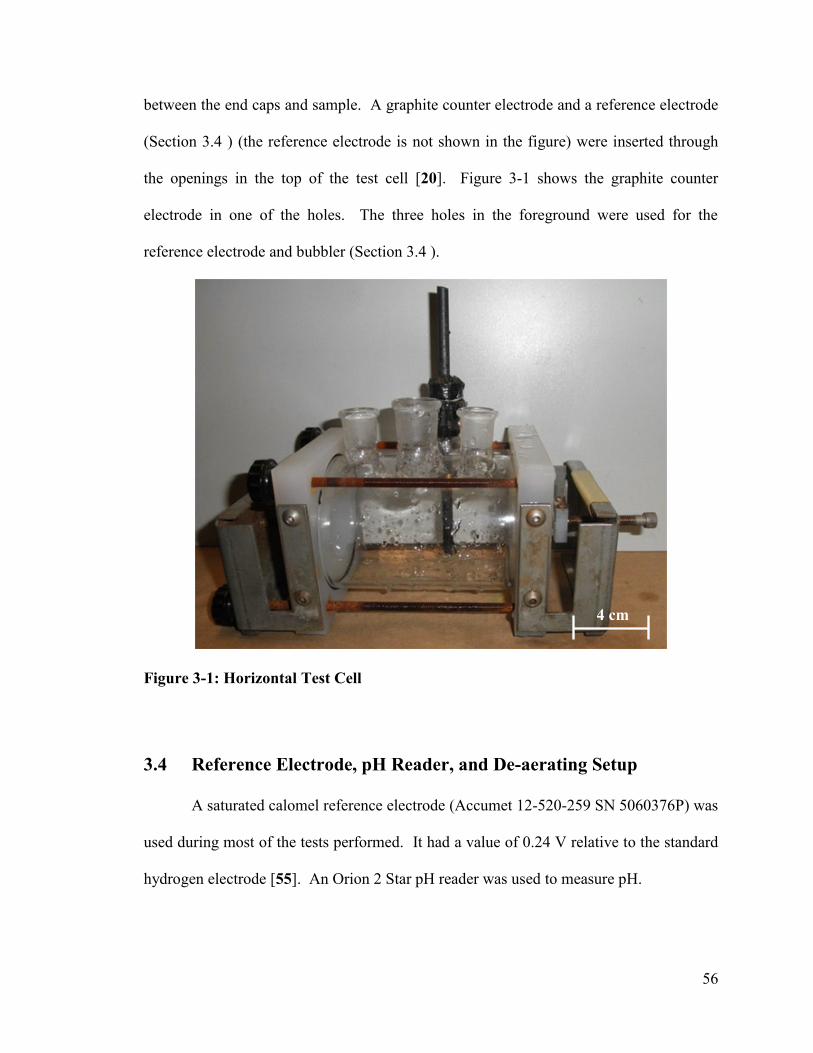
56

between the end caps and sample. A graphite counter electrode and a reference electrode

(Section 3.4 ) (the reference electrode is not shown in the figure) were inserted through

the openings in the top of the test cell [20]. Figure 3-1 shows the graphite counter

electrode in one of the holes. The three holes in the foreground were used for the

reference electrode and bubbler (Section 3.4 ).

Figure 3-1: Horizontal Test Cell

3.4 Reference Electrode, pH Reader, and De-aerating Setup

A saturated calomel reference electrode (Accumet 12-520-259 SN 5060376P) was

used during most of the tests performed. It had a value of 0.24 V relative to the standard

hydrogen electrode [55]. An Orion 2 Star pH reader was used to measure pH.

4 cm

57

All de-aeration was completed using carbon dioxide gas (CO2) or a combination

of CO2 and dry ice. In this thesis, de-aeration means to displace the dissolved oxygen

within a solution with CO2. The CO2 cylinder was connected by a tube to a sintered glass

frit. The sintered glass frit was placed in a flask containing water. The flask had two

openings. The first opening had a tube that lead from the cylinder to the flask. The

second opening had a tube that lead from the flask to the test cell. The end of this tube

was also attached to a sintered glass frit. Sintered glass frits were used as bubblers

because they create small bubbles with large surface areas; they de-aerate a solution

faster compared to a tube without a sintered glass frit. The intermediate beaker, placed

between the canister and test cell, was necessary. The initial gas from the canister was

dry. The intermediate beaker was used to moisten the initial gas from the canister. A dry

gas entering the test cell would remove moisture from the solution, which would cause

the volume of the solution to decrease and alter the concentration.

CO2 was bubbled for a minimum of 10 minutes, after which the CO2 gas was

turned off and test cell was sealed. Some tests were performed with CO2 bubbling during

the measurement, as indicated. Aerated solutions in this thesis were exposed to the

atmosphere so that the dissolved gases in solution were in equilibrium with the

atmosphere. De-aerated solutions were aerated by pouring the solution in and out of the

test cell three times; additional mixing did not alter the results.

3.5 Data Acquisition Equipment

Two different data acquisitions systems were used. The first system was a

Solartron 1287 potentiostat with a Solartron 1255 gain/phase analyzer. Different

58

software was used depending on the type of experiment and the equipment used. For EIS

tests using the Solartron, Zplot (version 3.2c) was used to run the test and ZView (version

3.2d) to view the results. When the Solartron was used for DC polarization tests

(specifically cyclic voltammetry tests), CorrWare (3.2c) was used to run the tests and

CorrView (3.2d) to view the results. The second system was a Gamry PC4/300. Gamry

Framekwork (4.35) was used to run both EIS and DC polarization (specifically cyclic

voltammetry) tests and EchemAnalyst (5.3) was used for viewing.

The Gamry system had an upper impedance limit (open circuit) of 1012

Ω at 100

mHz. The Solartron system had an upper impedance limit of 109 Ω at 100 mHz. In

general, the impedance and phase angle measurements would vary slowly with

frequency, however, below 200 Hz the measurements would sometimes vary rapidly,

appearing as noise and spikes in the spectra [8].

The explanation for the noise and spikes depends on how close the impedance

measurements were to the limits of the data acquisition equipment. When the impedance

measurements were close to the limit of detection, the spikes were considered to be noise,

otherwise, the spikes were considered to be real. In addition, when phase angles spiked

into positive values, this was interpreted as an indication that the underlying aluminum

was corroding (Section 2.1.4). The spikes do not appear at higher frequencies, but do

appear at lower frequencies, consistent with the rates of corrosion reactions [49].

3.6 Solutions

Hydrochloric acid solutions (HCl) (Anachemia, UN# 1789, CAS# 7647-01-0,

Lot# 210187), potassium chloride (KCl) (Bioshop, CAS# 7447-40-7, Lot# 1b19806), and

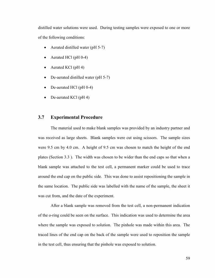
59

distilled water solutions were used. During testing samples were exposed to one or more

of the following conditions:

Aerated distilled water (pH 5-7)

Aerated HCl (pH 0-4)

Aerated KCl (pH 4)

De-aerated distilled water (pH 5-7)

De-aerated HCl (pH 0-4)

De-aerated KCl (pH 4)

3.7 Experimental Procedure

The material used to make blank samples was provided by an industry partner and

was received as large sheets. Blank samples were cut using scissors. The sample sizes

were 9.5 cm by 4.0 cm. A height of 9.5 cm was chosen to match the height of the end

plates (Section 3.3 ). The width was chosen to be wider than the end caps so that when a

blank sample was attached to the test cell, a permanent marker could be used to trace

around the end cap on the public side. This was done to assist repositioning the sample in

the same location. The public side was labelled with the name of the sample, the sheet it

was cut from, and the date of the experiment.

After a blank sample was removed from the test cell, a non-permanent indication

of the o-ring could be seen on the surface. This indication was used to determine the area

where the sample was exposed to solution. The pinhole was made within this area. The

traced lines of the end cap on the back of the sample were used to reposition the sample

in the test cell, thus ensuring that the pinhole was exposed to solution.

60

Pinholes were created with a mathematical compass or sewing needle. The

following sewing needle sizes were used: 70/10, 80/12, 90/14. The first number in

sewing needle sizes is the approximate diameter of the needle shaft (before any

reinforcements to the needle shaft). A needle designated as 70 would mean the diameter

of the needle is 0.7 mm. Needle sizes do not include the diameter of the needle tip.

The force required to create a pinhole depended on the instrument used. A

sharper instrument, like a sewing needle, damaged a sample more readily than a blunter

instrument, such as the mathematical compass. All pinholes were created by hand. It

was relatively easy to scratch the surface of a sample with a sewing needle. Care had to

be taken to use enough force to go through the coating, but not enough to go too deep

into the metal. The pinhole could be seen with the naked eye. The force used ranged

from 3.4 N to 6.9 N, which was determined by placing samples on a balance and

recording the force required to make a pinhole without visible damage to the metal

underneath the coating.

The samples were easily scratched and damaged by other objects, including other

samples. Care had to be taken while handling and storing samples. Samples were carried

by holding the edges. A tissue was used to wipe the surface of a sample clean. When not

in use, samples were stored individually in a plastic sleeve (photo album).

Only enough liquid to cover the exposed surface of a sample was poured into the

test cell. A test cell filled close to the top would have caused the liquid to overflow when

the solution was de-aerated (Section 3.4 ).

The first few steps were the same for all samples. A blank sample was placed in

distilled water. An EIS test was used to determine if there was any existing damage. If

61

there were signs of pre-existing defects, e.g, scratches caused by poor handling or

storage, the sample was discarded or a different area of the same sample was tested.

Figure 3-2 shows the results for a sample that was considered to not have any

major pre-existing defects which would alter the results of future tests. In these results

the impedance appeared as a relatively straight line, with a slope of -1, which reached

approximately 1010

Ω at low frequencies. The phase angle stayed at approximately -90°,

except at frequencies below a few Hertz.

Figure 3-2: A Good Blank Sample Containing No Measurable Pre-existing Defects

-200

-150

-100

-50

0

50

100

150

200

1E+00

1E+01

1E+02

1E+03

1E+04

1E+05

1E+06

1E+07

1E+08

1E+09

1E+10

1E+11

1E-02 1E-01 1E+00 1E+01 1E+02 1E+03 1E+04 1E+05

Ph

ase

An

gle

(°)

|Z|

(Ω)

Frequency (Hz)

|Z|

Phase Angle

62

Figure 3-3 shows the EIS test results for a blank sample that was considered to

have pre-existing defects. The impedance at low frequencies is resistive and not

capacitive; the slope in the impedance plot is closer to 0 than -1. In addition, the

impedance falls short of 1010

Ω seen in Figure 3-2 for a good blank sample. The

departure of the phase angle from -90° is much more apparent at low frequencies.

Figure 3-3: A Poor Blank Sample Containing Pre-existing Defects

Once a blank sample was tested and determined to have no measurable pre-

existing defects, a pinhole was created. The next step was another EIS test in distilled

water to determine if the pinhole penetrated the coating. If the EIS results were similar to

-200

-150

-100

-50

0

50

100

150

200

1E+00

1E+01

1E+02

1E+03

1E+04

1E+05

1E+06

1E+07

1E+08

1E+09

1E+10

1E+11

1E-02 1E-01 1E+00 1E+01 1E+02 1E+03 1E+04 1E+05

Ph

ase

An

gle

(°)

|Z|

(Ω)

Frequency (Hz)

|Z|

Phase Angle

63

the results for a good blank sample, the sample was discarded, or the pinhole was

reworked. If the EIS results were different, the sample was considered for further study

with EIS or cyclic voltammetry.

EIS tests used a frequency range from 105 Hz to 10

-1 Hz. Tests were performed

using an AC excitation voltage of 20 mV [8]. Sample area size was set to 1 cm2. The

DC polarization test used was a cyclic potentiodynamic test, also known as cyclic

voltammetry. The DC tests used a scan rate of 20 mV/s and a rate of 50 mV/point, which

were determined by maximizing the number of data points and minimizing the duration

of the test to minimize the degradation of the sample during the test. The potential range

for a cyclic voltammetry test was based on the Pourbaix diagram for aluminum. Potential

ranges were selected to ensure the major characteristics of an Evans diagram were seen,

if they were to occur (Section 2.3.2). The largest range used was -3 V to 2.5 V, and the

smallest was -1 V to 1 V.

64

Chapter 4 Results of Experiments

This section will go over the major results observed throughout the conducted

tests. All figure captions state which data acquisition equipment was used to obtain the

results; for results obtained using the Gamry, the figure caption will include (Gamry) at

the end, and for the Solartron, (Solartron) will appear at the end.

4.1 Effect of pH on Corrosion

This section will describe a series of tests where pH was altered, back and forth

between neutral and acidic conditions; it is divided by sample, Sample A and Sample B,

where each section describes the series of tests using its respective sample.

4.1.1 Sample A

Distilled Water (pH 7)

The pinhole in Sample A was created using the point of a mathematical compass,

as described in Section 3.7 . The Bode plot and Nyquist plot results in distilled water (pH

7) can be seen in Figure 4-1 and Figure 4-2. The plots suggest that the pinhole through

the coating was sufficiently large to cause the underlying aluminum to corrode; for

instance, the Bode plot contains positive phase angles and an impedance with a positive

slope at low frequencies (Section 2.1.4). Similarly, the Nyquist plot shows positive

imaginary impedance (Section 2.1.3). Positive phase angles, imaginary impedance, and

slopes at low frequencies are indications of active corrosion. In addition, the Bode plot in

Figure 4-1 resembles Figure 3-3 more than Figure 3-2; for instance, the impedance of the

coating is not capacitive below 20 Hz and the impedance at lower frequencies is below

65

107 Ω, which is indicative of a bad coating (Section 2.6.2). The lack of integrity of the

coating can also be seen in the cyclic voltammetry results shown in Figure 4-3. If the

coating were good, then the corrosion of the underlying aluminum would not be visible

and the current would not increase with applied DC voltage (Section 2.3.2). In Figure

4-3, as the DC potential is increased above the corrosion potential, the current density

increases initially, then it slows down, suggesting passivation. With further increase in

the potential, pitting occurs in the transpassive region. As the potential is decreased, the

current density decreases as the passivation potential is reached (Section 2.3.2). This

behaviour with applied DC potential is consistent with the corrosion of aluminum and not

the behaviour expected of a good coating (Section 2.3.2).

66

Figure 4-1: EIS Bode Plot Results in Distilled Water (pH 7) for Sample A

Containing a Pinhole (Gamry)

-100

-80

-60

-40

-20

0

20

1E+00

1E+01

1E+02

1E+03

1E+04

1E+05

1E+06

1E+07

1E+08

1E-02 1E-01 1E+00 1E+01 1E+02 1E+03 1E+04 1E+05 1E+06

Ph

ase

An

gle

(°)

|Z|

(Ω)

Frequency (Hz)

|Z|

Phase Angle

67

Figure 4-2: EIS Nyquist Plot Results in Distilled Water (pH 7) for Sample A

Containing a Pinhole (Gamry)

-5E+06

0E+00

5E+06

1E+07

2E+07

2E+07

3E+07

3E+07

4E+07

-5E+06 5E+06 2E+07 3E+07 4E+07

-Z''

(Ω)

Z' (Ω)

68


Potential Range: -2 V to +2 V (Gamry)

Distilled Water (pH 7) → HCl (pH 0)

When the solution in the test cell was changed to HCl (pH 0), Figure 4-4 shows

that the coating is now behaving as a good coating: the coating is capacitive and goes to

high impedances at low frequencies, no positive phase angles, and no positive slopes.

The Nyquist plot, seen in Figure 4-5, appears as an almost vertical line along the axis,

with no positive imaginary impedance. In contrast to Figure 4-3, Figure 4-6 shows

currents at the limit of detection of the instrument that are independent of the applied DC

voltage (Section 2.3.2). The implication is that changing the pH from 7 to 0 transformed

a bad coating, with a pinhole, into a good coating.

-2

-1.5

-1

-0.5

0

0.5

1

1.5

2

1.0E-11 1.0E-10 1.0E-09 1.0E-08 1.0E-07 1.0E-06 1.0E-05

Po

ten

tial

(V

vs

Vre

f)

I (A/cm2)

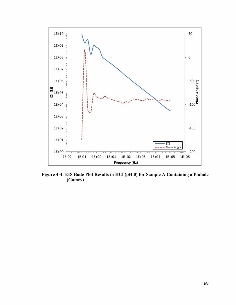
69

Figure 4-4: EIS Bode Plot Results in HCl (pH 0) for Sample A Containing a Pinhole

(Gamry)

-200

-150

-100

-50

0

50

1E+00

1E+01

1E+02

1E+03

1E+04

1E+05

1E+06

1E+07

1E+08

1E+09

1E+10

1E-02 1E-01 1E+00 1E+01 1E+02 1E+03 1E+04 1E+05 1E+06

Ph

ase

An

gle

(°)

|Z|

(Ω)

Frequency (Hz)

|Z|

Phase Angle

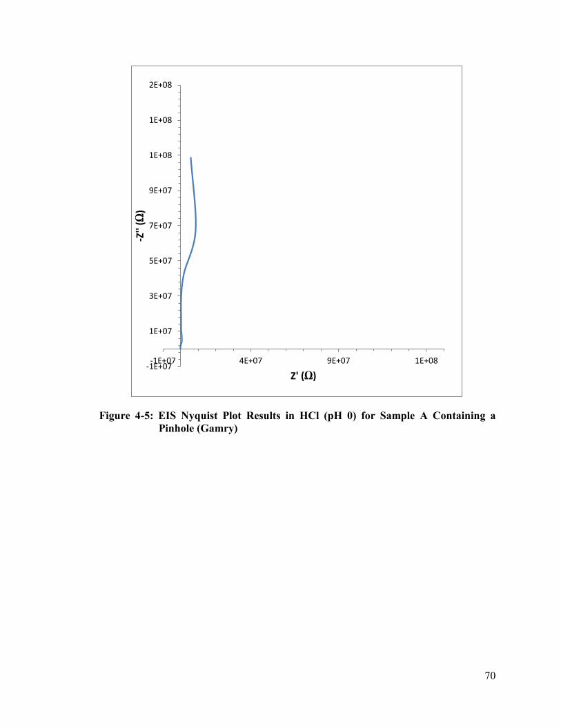
70

Figure 4-5: EIS Nyquist Plot Results in HCl (pH 0) for Sample A Containing a

Pinhole (Gamry)

-1E+07

1E+07

3E+07

5E+07

7E+07

9E+07

1E+08

1E+08

2E+08

-1E+07 4E+07 9E+07 1E+08

-Z''

(Ω)

Z' (Ω)

71

Figure 4-6: Cyclic Voltammetry Results for Sample A in HCl (pH 0). Potential

Range: -2 V to +2 V (Gamry)

HCl (pH 0) → HCl (pH 3.8)

An HCl solution with a pH of 3.8 (distilled water acidified with HCl) was used to

investigate the behaviour of the coating between the „bad‟ pH 7 results seen in Figure 4-3

and the „good‟ pH 0 results seen in Figure 4-6. A cyclic voltammetry test was performed

and the results can be seen in Figure 4-7. The sample started off with the same current

density as in HCl (pH 0) (10-11

A/cm2), and began to increase by two orders of magnitude

at -0.5 V. On the return scan, after reaching 0.9 V, the current density increased by five

orders of magnitude (this point has been highlighted by a red circle in the Figure). As the

voltage was reduced further, the polarization plot had the characteristics of corroding

metal, including a passivation potential, similar to those shown in Figure 4-3.

-2

-1.5

-1

-0.5

0

0.5

1

1.5

2

1.0E-13 1.0E-12 1.0E-11 1.0E-10 1.0E-09

Po

ten

tial

(V

vs

Vre

f)

I(A/cm2)

72

The test was repeated with the same sample under the same conditions. The

results are shown in Figure 4-8. This time the sample only briefly stayed at a current

density of 10-11

A/cm2 and then began behaving like corroding aluminum.

Figure 4-7: Cyclic Voltammetry Results for Sample A in HCl (pH 3.8). Potential

Range: -2 V to +2 V (Gamry)

-2

-1.5

-1

-0.5

0

0.5

1

1.5

2

1.0E-13 1.0E-12 1.0E-11 1.0E-10 1.0E-09 1.0E-08 1.0E-07 1.0E-06 1.0E-05

Po

ten

tial

(V

vs

Vre

f)

I (A/cm2)

Passivation potential

73

Figure 4-8: Second Cyclic Voltammetry Results for Sample A in HCl (pH 3.8).


HCl (pH 3.8) → HCl (pH 0)

In the next test, the pH was changed from 3.8, which was the value in previous test, to 0.

Cyclic voltammetry results are shown in Figure 4-9. The current density started at 10-11

A/cm2 and increased by factor of 6 on the upward scan. The curve also returned on the

passivation side, which is the behaviour of an intact sample.

-2

-1.5

-1

-0.5

0

0.5

1

1.5

2

1.0E-12 1.0E-11 1.0E-10 1.0E-09 1.0E-08 1.0E-07 1.0E-06 1.0E-05 1.0E-04

Po

ten

tial

(V

vs

Vre

f)

I (A/cm2)

74

Figure 4-9: Second Cyclic Voltammetry Results for Sample A in HCl (pH 0).



The solution in the test cell was changed to HCl (pH 3.8). Another cyclic

voltammetry test was performed, and the results are shown in Figure 4-10. At the

beginning of the test, corrosion of the underlying aluminum was recorded; the corrosion

potential can be seen. The aluminum was able to passivate, after reaching the corrosion

potential, until 0.7 V on the forward scan. After this point in the test, the aluminum

appeared to go through stages of corrosion and passivation as the current density jumped

between high values (10-7

A/cm2) and low values closer to the limit of detection of the

equipment (10-10

A/cm2). On the return scan, at 0.5 V the current density began to

increase and the polarization curve began to resemble corroding aluminum again; a

passivation potential appeared on the return sweep. Based on the Pourbaix diagram, it

-2

-1.5

-1

-0.5

0

0.5

1

1.5

2

1.0E-12 1.0E-11 1.0E-10

Po

ten

tial

(V

vs

Vre

f)

I (A/cm2)

75

was possible the aluminum was able to passivate at pH 3.8, or the coating had some

influence on impeding the corrosion of aluminum.

Figure 4-10: Third Cyclic Voltammetry Results for Sample A in HCl (pH 3.8).


HCl (pH 3.8) → Distilled Water (pH 7)

The solution was switched to distilled water (pH 7). A cyclic voltammetry test

was performed, with the results shown in Figure 4-11. The polarization curve was

similar to the results expected when the underlying aluminum was corroding; a corrosion

potential appeared on the forward scan, followed by passivation between -0.9V and 1 V,

pitting from 1 V until the return scan where the aluminum passivated again. The

aluminum appeared to corrode again after 0.3 V on the return scan, and the passivation

-2

-1.5

-1

-0.5

0

0.5

1

1.5

2

1.0E-12 1.0E-11 1.0E-10 1.0E-09 1.0E-08 1.0E-07 1.0E-06

Po

ten

tial

(V

vs

Vre

f)

I (A/cm2)

76

potential appeared. The results had typical features of aluminum corrosion and

passivation at pH 7.

Figure 4-11: Second Cyclic Voltammetry Results for Sample A in Distilled Water

(pH 7). Potential Range: -2 V to +2 V (Gamry)

Distilled Water (pH 7) → Distilled Water (pH 7) 9 Days Later

After the previous test, Sample A was cleaned with distilled water, dried, and left

exposed to air for 9 days. The first test conducted upon returning was an EIS test. Figure

4-12 shows the Bode plot. The results show that the underlying aluminum was corroding

and that the coating was behaving as a bad coating; positive angles and an impedance

below 107 Ω at low frequencies can be seen in the Bode plot. Figure 4-13 shows the

Nyquist plot for the EIS test; two semi-circles can be seen, as well as positive imaginary

-2

-1.5

-1

-0.5

0

0.5

1

1.5

2

1.0E-11 1.0E-10 1.0E-09 1.0E-08 1.0E-07 1.0E-06

Po

ten

tial

(V

vs

Vre

f)

I (A/cm2)

77

impedance at low frequencies. Two cyclic voltammetry tests were performed next, the

results can be seen in Figure 4-14 and Figure 4-15.

Figure 4-12: EIS Bode Plot Results in Distilled Water (pH 7) for Sample A

Containing a Pinhole. Performed 9 days after Initial Tests (Solartron)

-100

-80

-60

-40

-20

0

20

40

60

1E+00

1E+01

1E+02

1E+03

1E+04

1E+05

1E+06

1E+07

1E-02 1E-01 1E+00 1E+01 1E+02 1E+03 1E+04 1E+05

Ph

ase

An

gle

(°)

|Z|

(Ω)

Frequency (Hz)

|Z|

Phase Angle

78

Figure 4-13: EIS Nyquist Plot Results in Distilled Water (pH 7) for Sample A

Containing a Pinhole. Performed 9 days after Initial Tests (Solartron)

-1E+06

0E+00

1E+06

2E+06

3E+06

4E+06

5E+06

6E+06

-1E+06 0E+00 1E+06 2E+06 3E+06 4E+06 5E+06 6E+06

-Z''

(Ω)

Z' (Ω)

79


Performed 9 days after Initial Tests. Potential Range: -2 V to +2 V

(Solartron)

-2

-1.5

-1

-0.5

0

0.5

1

1.5

2

1.0E-10 1.0E-09 1.0E-08 1.0E-07 1.0E-06

Po

ten

tial

(V

vs

Vre

f)

I (A/cm2)

80

Figure 4-15: Cyclic Voltammetry Test Results for Sample A in Distilled Water (pH

7). Performed 9 days after Initial Tests. Potential Range: -3 V to +3

(Solartron)

Both tests showed that the underlying aluminum was corroding; corrosion potential,

pitting, and passivation potential can all be seen. The current density changed with a

change in voltage, indicative of the coating behaving as a bad coating. Pitting that

occurred in the first cyclic voltammetry test, results shown in Figure 4-14, may have

damaged the sample enough so that the second cyclic voltammetry test results differed

slightly, seen in Figure 4-15. The second test began at a higher current density (5·10-7

A/cm2 versus 2.5·10

-7 A/cm

2), and also the during pitting a higher current density was

reached (2·10-6

A/cm2 versus 3·10

-7 A/cm

2).

-3

-2

-1

0

1

2

3

1.0E-11 1.0E-10 1.0E-09 1.0E-08 1.0E-07 1.0E-06 1.0E-05

Po

ten

tial

(V

vs

Vre

f)

I (A/cm2)

81


The distilled water (pH 7) was switched to HCl (pH 0). An EIS test was

completed, and the Bode plot can be seen in Figure 4-16. The coating was now behaving

as a good coating, even after being left exposed to air for 9 days; the coating was

capacitive, the impedance reached high values (above 109 Ω) at low frequencies, and

there were no positive phase angles (excluding noise). The Nyquist plot, shown in Figure

4-17, also implied that Sample A had a good coating again; no positive imaginary

impedance can be seen, and the curve follows a vertical path along the axis.

Figure 4-16: EIS Bode Plot Results in HCl (pH 0) for Sample A Containing a

Pinhole. Performed 9 days after Initial Tests (Solartron)

-150

-100

-50

0

50

100

150

200

1E+00

1E+01

1E+02

1E+03

1E+04

1E+05

1E+06

1E+07

1E+08

1E+09

1E+10

1E-02 1E-01 1E+00 1E+01 1E+02 1E+03 1E+04 1E+05

Ph

ase

An

gle

(°)

|Z|

(Ω)

Frequency (Hz)

|Z|

Phase Angle

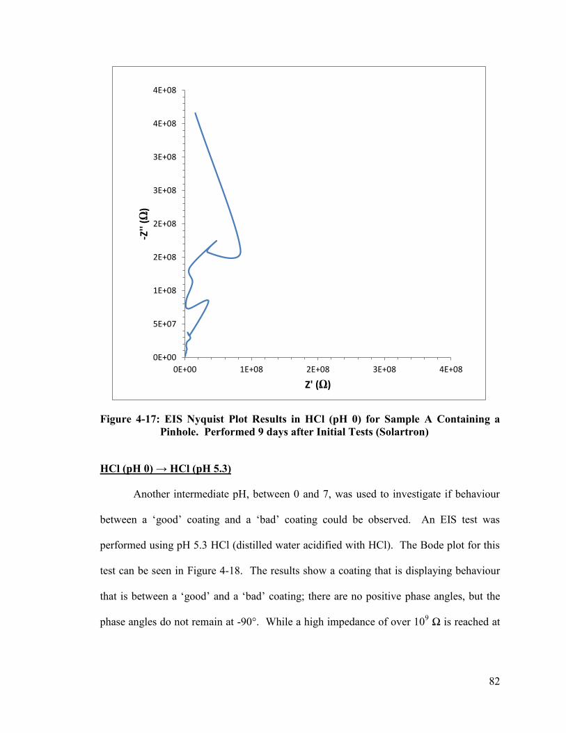
82

Figure 4-17: EIS Nyquist Plot Results in HCl (pH 0) for Sample A Containing a



Another intermediate pH, between 0 and 7, was used to investigate if behaviour

between a „good‟ coating and a „bad‟ coating could be observed. An EIS test was

performed using pH 5.3 HCl (distilled water acidified with HCl). The Bode plot for this

test can be seen in Figure 4-18. The results show a coating that is displaying behaviour

that is between a „good‟ and a „bad‟ coating; there are no positive phase angles, but the

phase angles do not remain at -90°. While a high impedance of over 109 Ω is reached at

0E+00

5E+07

1E+08

2E+08

2E+08

3E+08

3E+08

4E+08

4E+08

0E+00 1E+08 2E+08 3E+08 4E+08

-Z''

(Ω)

Z' (Ω)

83

lower frequencies, the coating does not behave as a capacitor since the line does not have

a slope of -1 throughout the entire test.

Figure 4-18: EIS Bode Plot Results in HCl (pH 5.3) for Sample A Containing a


The same sample was then left overnight in distilled water (pH 7).

HCl (pH 5.3) → Distilled Water (pH 7) Overnight → HCl (pH 2)

The next solution used was HCl (pH 2), after the sample had been left soaking in

distilled water (pH 7) overnight. An EIS test was performed, and the Bode plot for this

test can been seen in Figure 4-19. The coating was now behaving as a bad coating in low

-150

-100

-50

0

50

100

150

1E+00

1E+01

1E+02

1E+03

1E+04

1E+05

1E+06

1E+07

1E+08

1E+09

1E+10

1E-02 1E-01 1E+00 1E+01 1E+02 1E+03 1E+04 1E+05

Ph

ase

An

gle

(°)

|Z|

(Ω)

Frequency (Hz)

|Z|

Phase Angle

84

pH solutions; the underlying aluminum was corroding and could be detected during the

EIS test. The phase angles were close to 0° or positive, and the impedance was low at

lower frequencies, below 107 Ω and indicative of a bad coating. After the sample had

been soaked overnight in distilled water (pH 7), all tests (no matter which pH solution

was used) produced results where the underlying aluminum was corroding.

Figure 4-19: EIS Bode Plot Results in HCl (pH 2) for Sample A Containing a

Pinhole, Left Overnight in Distilled Water (pH 7) (Solartron)

An optical microscope was used to find the size of the pinhole after all testing was

complete. Figure 4-20 shows the microscopic image of the pinhole in Sample A taken at

200x magnification. The pinhole had a size of 250 μm by 290 μm.

-100

-80

-60

-40

-20

0

20

40

1E+00

1E+01

1E+02

1E+03

1E+04

1E+05

1E-02 1E-01 1E+00 1E+01 1E+02 1E+03 1E+04 1E+05

Ph

ase

An

gle

(°)

|Z|

(Ω)

Frequency (Hz)

|Z|

Phase Angle

85

Figure 4-20: Microscopic Image of Sample A Pinhole (Post-experiments, 200x

Magnification)

4.1.2 Sample B

Sample B contained a pinhole which was made with a 70/10 sewing needle

(Section 3.7 ). A microscopic image was taken of the pinhole before conducting any

experiments. The pinhole, seen in Figure 4-21, measured approximately 85 μm by 53

μm. The image shows that the sewing needle had penetrated the coating, but also that the

needle had created a lip around the pinhole by pushing the coating back.

86

Figure 4-21: Microscopic Image of Sample B Pinhole (Pre-experiments, 200x

Magnification)

Distilled Water (pH 7)

The first solution used was distilled water (pH 7). A Bode plot for an EIS test can

be seen in Figure 4-22. The results are indicative of corroding aluminum; for instance,

the phase angles are not at -90°, and the impedance is low (less than 107

Ω) at low

frequencies. This suggests that the coating is behaving like a bad coating.

87

Figure 4-22: EIS Bode Plot Results in Distilled Water (pH 7) for Sample B

Containing a Pinhole (Solartron)


The solution was then switched to HCl (pH 1). The Bode plot for an EIS test is

shown in Figure 4-23. The coating was now behaving as a good coating; the impedance

reached over 109 Ω at lower frequencies, and there were no positive phase angles.

-200

-150

-100

-50

0

50

100

150

200

1E+00

1E+01

1E+02

1E+03

1E+04

1E+05

1E+06

1E+07

1E+08

1E-02 1E-01 1E+00 1E+01 1E+02 1E+03 1E+04 1E+05

Ph

ase

An

gle

(°)

|Z|

(Ω)

Frequency (Hz)

|Z|

Phase Angle

88

Figure 4-23: EIS Bode Plot Results in HCl (pH 1) for Sample B Containing a

Pinhole (Solartron)

Further testing (EIS and cyclic voltammetry) was conducted on Sample B by

switching back and forth between distilled water (pH 7) and HCl (pH 1).

HCl (pH 1) → Distilled Water (pH 7) → HCl (pH 1)

Figure 4-24 shows two other tests that were conducted. The solution was

switched from HCl (pH 1), to distilled water (pH 7), and then back to HCl (pH 1). The

figure shows that the aluminum was corroding (impedance below 107 Ω at low

-120

-100

-80

-60

-40

-20

0

1E+00

1E+01

1E+02

1E+03

1E+04

1E+05

1E+06

1E+07

1E+08

1E+09

1E+10

1E-02 1E-01 1E+00 1E+01 1E+02 1E+03 1E+04 1E+05

Ph

ase

An

gle

(°)

|Z|

(Ω)

Frequency (Hz)

|Z|

Phase Angle

89

frequencies) in distilled water (pH 7), but then the coating began to behave as a good

coating (impedance near the limit of the equipment at low frequencies) in HCl (pH 1).

Figure 4-24: Two EIS Bode Plot Results for Sample B Containing a Pinhole in

(Solartron): Distilled Water (pH 7) (Left) and HCl (pH 1) (Right)

Spikes in impedance and phase angle appeared in both test results shown in Figure 4-24.

For the test conducted in distilled water (pH 7), the spikes were considered to be real

(corrosion) due to the low impedance at low frequencies (Section 3.5 ). For the test

conducted in HCl (pH 1), the spikes that appeared where the impedance was capacitive

(-1 slope) were considered to be noise. Between 0.5 Hz and 0.1 Hz, the spikes in

impedance and phase angle appeared to no longer be noise, but signs of the underlying

aluminum corroding (the impedance is not at the limit of detection of the equipment at

low frequencies). To verify that the underlying aluminum was now corroding, several

EIS and cyclic voltammetry tests were conducted. These tests were performed using both

the Solartron and the Gamry to verify that one of the machines was not malfunctioning.

-200

-150

-100

-50

0

50

100

150

200

250

1E+00

1E+01

1E+02

1E+03

1E+04

1E+05

1E+06

1E+07

1E+08

1E+09

1E-02 1E-01 1E+00 1E+01 1E+02 1E+03 1E+04 1E+05P

has

e A

ngl

e (°)

|Z|

(Ω)

Frequency (Hz)

-200

-150

-100

-50

0

50

100

150

200

250

1E+00

1E+01

1E+02

1E+03

1E+04

1E+05

1E+06

1E+07

1E+08

1E+09

1E-02 1E-01 1E+00 1E+01 1E+02 1E+03 1E+04 1E+05

Ph

ase

An

gle

(°)

|Z|

(Ω)

Frequency (Hz)

90

As an aside, it is important to note the difference in impedance at high frequencies

between the two results shown in Figure 4-24. The resistive behaviour of the impedance

at high frequencies in distilled water (pH 7) is the resistance of the solution, Rsol. Rsol

does not depend on frequency. The appearance of Rsol in the plot can be explained using

the Randles circuit model (Figure 2-16) and the circuit model for a failed coating (Figure

2-17). At high frequencies, the impedance of a capacitor is low (Table 2-1). Current

follows the path of least resistance, which in Figure 2-16 and Figure 2-17 at high

frequencies would be the path containing Rsol and coating capacitance, Cc. Since the

magnitude of Rsol of distilled water dominates the magnitude of Cc, Rsol of distilled water

is visible at high frequencies in the results. Rsol of HCl is lower than the Rsol of distilled

water because the HCl solution contains more ions in solution; these ions create a path of

least resistance for the current in solution. Rsol of HCl is dominated by Cc and cannot be

seen in the results.

The last EIS test on Sample B in HCl (pH 1) was performed after several EIS and

cyclic voltammetry tests showed that the Solartron was not malfunctioning and the

aluminum was now corroding. Figure 4-25 shows the results of the next test. The

coating started to behaving as a bad coating in HCl (pH 1), allowing the underlying

aluminum to corrode; for instance, phase angles close to 0°, and the impedance becoming

independent of frequency starting at 2·108 Hz (resistive behaviour) are indications that

the aluminum is now corroding.

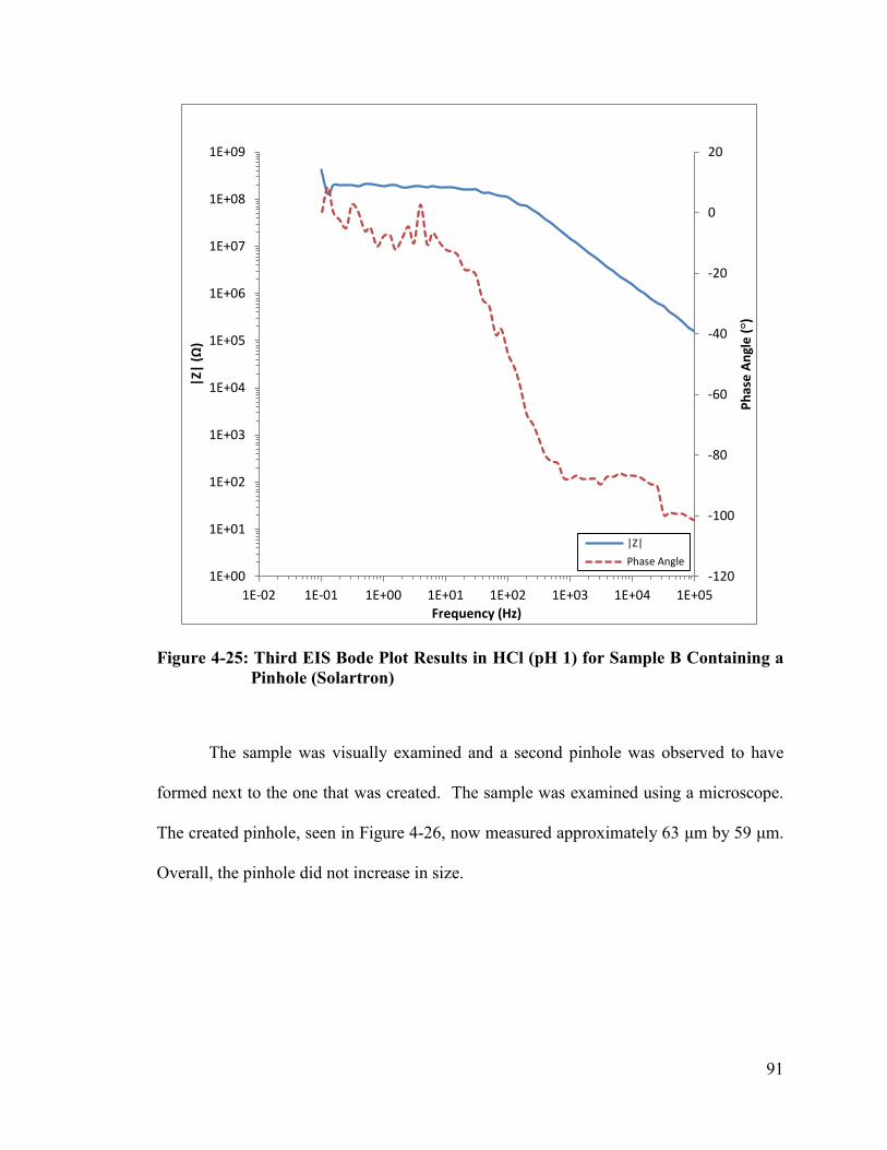
91

Figure 4-25: Third EIS Bode Plot Results in HCl (pH 1) for Sample B Containing a

Pinhole (Solartron)

The sample was visually examined and a second pinhole was observed to have

formed next to the one that was created. The sample was examined using a microscope.

The created pinhole, seen in Figure 4-26, now measured approximately 63 μm by 59 μm.

Overall, the pinhole did not increase in size.

-120

-100

-80

-60

-40

-20

0

20

1E+00

1E+01

1E+02

1E+03

1E+04

1E+05

1E+06

1E+07

1E+08

1E+09

1E-02 1E-01 1E+00 1E+01 1E+02 1E+03 1E+04 1E+05

Ph

ase

An

gle

(°)

|Z|

(Ω)

Frequency (Hz)

|Z|

Phase Angle

92

Figure 4-26: Microscopic Image of Sample B Pinhole (Post-experiments, 200x

Magnification)

The damage that was observed, the new pinhole that had formed during testing, was also

observed with a microscope. The microscopic image can be seen in Figure 4-27. The

damage that had formed, which measured approximately 110 μm by 100 μm, was almost

double the size of the created pinhole, both before and after testing.

Figure 4-27: Microscopic Image of Sample B Damage (Post-experiment, 200x

Magnification)

93

4.2 Effect of De-Aeration of Solution Using Carbon Dioxide

This section will describe tests where the solution in the test cell was aerated, and

de-aerated using carbon dioxide gas (CO2). Aerated solutions have their dissolved gases

in equilibrium with atmospheric air. In the de-aerated solutions, the aerated dissolved

gases have been replaced with CO2 (Section 3.4 ). Unless otherwise stated, the same

sample was used during testing. The pH of solution was not altered during these tests.

4.2.1 Sample C

Aerated Distilled Water (pH 7)

A pinhole was made in Sample C using a mathematical compass (Section 3.7 ).

Figure 4-28 shows the Bode plot for an EIS test conducted in aerated distilled water (pH

7). The results are indicative of corroding aluminum and a bad coating; there are positive

phase angles, and the impedance at lower frequencies is below 107 Ω. The Nyquist plot

can be seen in Figure 4-29; it can be used to infer that the underlying aluminum was

corroding because of the appearance of positive imaginary impedances (Section 2.1.3).

94

Figure 4-28: EIS Bode Plot Results in Distilled Water (pH 7) for Sample C


-120

-100

-80

-60

-40

-20

0

20

40

60

1E+00

1E+01

1E+02

1E+03

1E+04

1E+05

1E+06

1E+07

1E-02 1E-01 1E+00 1E+01 1E+02 1E+03 1E+04 1E+05

Ph

ase

An

gle

(°)

|Z|

(Ω)

Frequency (Hz)

|Z|

Phase Angle

95

Figure 4-29: EIS Nyquist Plot Results in Distilled Water (pH 7) for Sample C


Aerated Distilled Water (pH 7) → De-aerated Distilled Water (pH 7)

The distilled water in the test cell was de-aerated using dry ice and by bubbling

carbon dioxide gas through the solution for 30 minutes (Section 3.4 ). An EIS test was

completed. Figure 4-30 shows the Bode plot. The coating is now behaving better than it

did in aerated distilled water (pH 7); compared to Figure 4-28, there are no more positive

phase angles and the impedance at lower frequencies went above 107 Ω (reaching 10

9 Ω).

It is not considered to be behaving as a good coating because the phase angles do not stay

at -90° and the impedance curve does not have a slope of -1 (capacitive behaviour). The

-7E+06

-5E+06

-3E+06

-1E+06

1E+06

3E+06

5E+06

7E+06

-1E+06 1E+06 3E+06 5E+06 7E+06-Z''

(Ω)

Z' (Ω)

96

Nyquist plot, seen in Figure 4-31, also can be used to infer that the coating was behaving

better than before; compared to Figure 4-29, there are no more full semi-circles or

positive imaginary impedances, but the curve does not follow the vertical axis and begins

to form part of a semi-circle.

Figure 4-30: EIS Bode Plot Results for Sample C Containing a Pinhole in De-

aerated Distilled Water (pH 7) (Solartron)

-100

-90

-80

-70

-60

-50

-40

-30

-20

-10

0

1E+00

1E+01

1E+02

1E+03

1E+04

1E+05

1E+06

1E+07

1E+08

1E+09

1E-02 1E-01 1E+00 1E+01 1E+02 1E+03 1E+04 1E+05P

has

e A

ngl

e (°)

|Z|

(Ω)

Frequency (Hz)

|Z|

Phase Angle

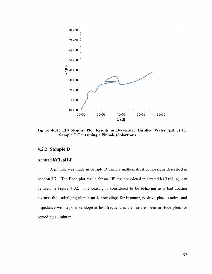
97

Figure 4-31: EIS Nyquist Plot Results in De-aerated Distilled Water (pH 7) for

Sample C Containing a Pinhole (Solartron)

4.2.2 Sample D

Aerated KCl (pH 4)

A pinhole was made in Sample D using a mathematical compass, as described in

Section 3.7 . The Bode plot result, for an EIS test completed in aerated KCl (pH 4), can

be seen in Figure 4-32. The coating is considered to be behaving as a bad coating

because the underlying aluminum is corroding; for instance, positive phase angles, and

impedance with a positive slope at low frequencies are features seen in Bode plots for

corroding aluminum.

0E+00

1E+08

2E+08

3E+08

4E+08

5E+08

6E+08

7E+08

8E+08

0E+00 2E+08 4E+08 6E+08 8E+08

-Z''

(Ω)

Z' (Ω)

98

Figure 4-32: EIS Bode Plot Results for Sample D Containing a Pinhole in KCl

(pH 4) (Solartron)

Aerated KCl (pH 4) → De-aerated KCl (pH 4)

The KCl solution in the test cell was de-aerated using carbon dioxide gas for 10

minutes, as described in Section 3.4 . An EIS test was conducted on this sample after de-

aerating the solution. The carbon dioxide gas was left bubbling into the solution during

the test. Figure 4-33 shows the Bode plot. From the Bode plot it can be inferred that the

coating is now behaving as a good coating, even with a pinhole exposing the underlying

aluminum. Compared to the previous results, seen in Figure 4-32, the Bode plot shown

in Figure 4-33 has features indicative of a good coating; for instance, the impedance is

-200

-150

-100

-50

0

50

100

150

200

1E+00

1E+01

1E+02

1E+03

1E+04

1E+05

1E+06

1E+07

1E+08

1E-02 1E-01 1E+00 1E+01 1E+02 1E+03 1E+04 1E+05

Ph

ase

An

gle

(°)

|Z|

(Ω)

Frequency (Hz)

|Z|

Phase Angle

99

high at low frequencies (almost reaching 1010

Ω at 0.1 Hz), and the phase angles are close

to -90°, except at low frequencies where the limit of detection for the equipment (Section

3.6 ) was reached and the data became noisy (large peaks).

Figure 4-33: EIS Bode Plot Results for Sample D Containing a Pinhole in De-

aerated KCl (pH 4) (Solartron)

4.3 Formation of Bubbles

This section will describe results where a bubble formed over the pinhole,

stopping the underlying aluminum from corroding. Unlike in the previous sections, the

pH was kept constant during these tests. Both aerated and de-aerated solutions were used

for these tests.

-150

-100

-50

0

50

100

150

1E+00

1E+01

1E+02

1E+03

1E+04

1E+05

1E+06

1E+07

1E+08

1E+09

1E+10

1E-02 1E-01 1E+00 1E+01 1E+02 1E+03 1E+04 1E+05

Ph

ase

An

gle

(°)

|Z|

(Ω)

Frequency (Hz)

|Z|

Phase Angle

100

4.3.1 Sample E

KCl (pH 4)

The pinhole in Sample E was created using a mathematical compass. An EIS test

was conducted using KCl (pH 4). The Bode plot showing the results for this test can be

seen in Figure 4-34. At the beginning of the test, starting at the high frequencies, the

underlying aluminum was corroding and the coating was behaving as a bad coating. The

impedance magnitude curve started with a slope of -1 at high frequencies, until it began

to roll over stating at 2·103 Hz until 40 Hz. The phase angle, between 2·10

3 Hz and 40

Hz, began to increase from -90° to -10°. When the test reached 40 Hz, the phase angle

dropped to -90° and the impedance resumed a -1 slope. At this time, a bubble had

formed over the pinhole on the surface of the sample, and could be seen visually. When

the test reached 1 Hz, this point during the test is shown as a dotted ellipse in the Bode

plot shown in Figure 4-34, the surface of the sample was quickly exposed to air by

shaking and tilting the test cell. After the bubble was removed, the Bode plot began to

resemble a plot for corroding aluminum; for instance, the impedance at low frequencies

dropped from above 108 Ω to below 10

5 Ω.

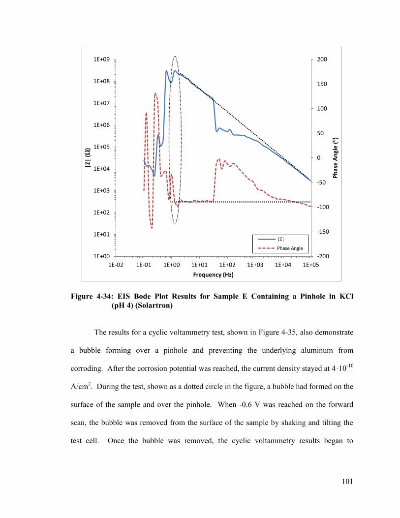
101

Figure 4-34: EIS Bode Plot Results for Sample E Containing a Pinhole in KCl

(pH 4) (Solartron)

The results for a cyclic voltammetry test, shown in Figure 4-35, also demonstrate

a bubble forming over a pinhole and preventing the underlying aluminum from

corroding. After the corrosion potential was reached, the current density stayed at 4·10-10

A/cm2. During the test, shown as a dotted circle in the figure, a bubble had formed on the

surface of the sample and over the pinhole. When -0.6 V was reached on the forward

scan, the bubble was removed from the surface of the sample by shaking and tilting the

test cell. Once the bubble was removed, the cyclic voltammetry results began to

-200

-150

-100

-50

0

50

100

150

200

1E+00

1E+01

1E+02

1E+03

1E+04

1E+05

1E+06

1E+07

1E+08

1E+09

1E-02 1E-01 1E+00 1E+01 1E+02 1E+03 1E+04 1E+05

Ph

ase

An

gle

(°)

|Z|

(Ω)

Frequency (Hz)

|Z|

Phase Angle

102

resemble corroding aluminum again; pitting and the passivation potential can be seen in

the results.

Figure 4-35: Cyclic Voltammetry Results for Sample E in KCl (pH 4). Potential

Range: -2.5 V to +3 V (Solartron)

4.3.2 Sample F

De-aerated Distilled Water (pH 7)

The pinhole in Sample F was made with a mathematical compass, as described in

Section 3.7 . The results for a cyclic voltammetry test in de-aerated distilled water (pH 7)

are shown in Figure 4-36. The solution was de-aerated for 30 minutes using CO2. The

results resemble typical corroding aluminum results (Section 2.3.2). During the reverse

scan, at 0.7 V, the current density decreased by 5 orders of magnitude. At this time

during the test, the surface of the sample was observed, without disturbing the test cell,

-3

-2

-1

0

1

2

3

1.0E-11 1.0E-10 1.0E-09 1.0E-08 1.0E-07 1.0E-06 1.0E-05 1.0E-04 1.0E-03

Po

ten

tial

(V

vs

Vre

f)

I (A/cm2)

103

and a bubble could be seen on the surface of the sample where the pinhole had been

made.

Figure 4-36: Cyclic Voltammetry Results for Sample F in De-aerated Distilled

Water (pH 7). Potential Range: -2.5 V to +3 V (Solartron)

An EIS test was performed in the same solution, de-aerated distilled water (pH 7),

without disturbing the test cell or removing the bubble. The Bode plot results are shown

in Figure 4-37. Using the results, it can be inferred that the underlying aluminum is no

longer corroding; high impedance at low frequencies (above 109 Ω at 0.1 Hz), and phase

angles close to -90° are not features of corroding aluminum.

-3

-2

-1

0

1

2

3

1.0E-13 1.0E-12 1.0E-11 1.0E-10 1.0E-09 1.0E-08 1.0E-07 1.0E-06 1.0E-05 1.0E-04

Po

ten

tial

(V

vs

Vre

f)

I (A/cm2)

104

Figure 4-37: EIS Bode Plot Results for Sample F Containing a Pinhole in De-aerated

Distilled Water (pH 7) (Solartron)

A second cyclic voltammetry test was performed without disturbing the bubble on the

surface of the sample. The results, shown in Figure 4-38, suggest that the underlying

aluminum is no longer corroding, and the coating is behaving as a good coating due to

the pinhole being blocked; the current density does not change as potential in increased

and decreased.

-120

-100

-80

-60

-40

-20

0

1E+00

1E+01

1E+02

1E+03

1E+04

1E+05

1E+06

1E+07

1E+08

1E+09

1E+10

1E-02 1E-01 1E+00 1E+01 1E+02 1E+03 1E+04 1E+05

Ph

ase

An

gle

(°)

|Z|

(Ω)

Frequency (Hz)

|Z|

Phase Angle

105

Figure 4-38: Second Cyclic Voltammetry Results for Sample F in De-aerated

Distilled Water (pH 7). Potential Range: -2.5 V to +3 V (Solartron)

After the second cyclic voltammetry test, the bubble was removed from the surface of the

sample (shaking and tilting the test cell and exposing the surface of the sample to air).

An EIS test was performed, and the Bode plot results can be seen in Figure 4-39. The

underlying aluminum is now corroding; for instance, the impedance at low frequencies in

the Bode plot is below 107 Ω, phase angles are positive, and the slope of the impedance

becomes positive at high frequencies.

-3

-2

-1

0

1

2

3

1.0E-10 1.0E-09 1.0E-08

Po

ten

tial

(V

vs

Vre

f)

I (A/cm2)

106

Figure 4-39: Second EIS Bode Plot Results for Sample F Containing a Pinhole in

De-aerated Distilled Water (pH 7) (Solartron)

A cyclic voltammetry test, with no bubble over the pinhole present, was performed. The

results are shown in Figure 4-40. The shape and features of the curve are indicative of

corroding aluminum; a corrosion potential occurs during the forward scan, the current

density increases as voltage increase during the forward scan, and a passivation potential

occurs during the reverse scan.

-60

-50

-40

-30

-20

-10

0

10

20

1E+00

1E+01

1E+02

1E+03

1E+04

1E+05

1E+06

1E-02 1E-01 1E+00 1E+01 1E+02 1E+03 1E+04 1E+05

Ph

ase

An

gle

(°)

|Z|

(Ω)

Frequency (Hz)

|Z|

Phase Angle

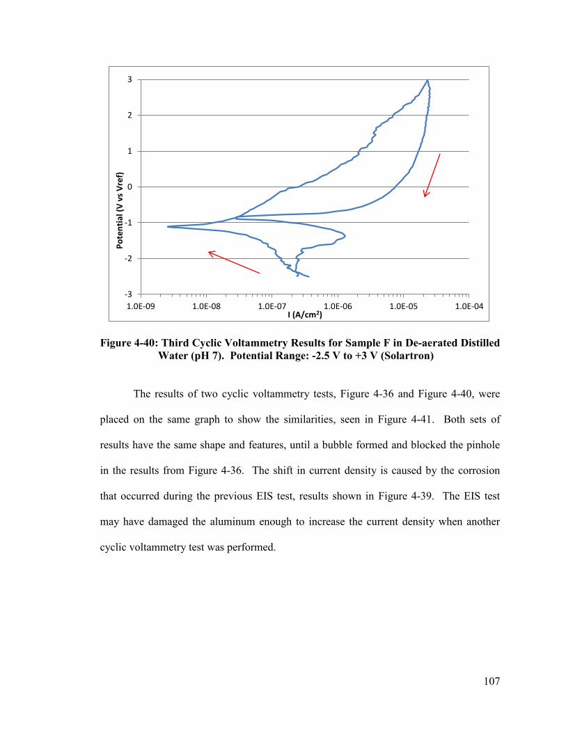
107

Figure 4-40: Third Cyclic Voltammetry Results for Sample F in De-aerated Distilled

Water (pH 7). Potential Range: -2.5 V to +3 V (Solartron)

The results of two cyclic voltammetry tests, Figure 4-36 and Figure 4-40, were

placed on the same graph to show the similarities, seen in Figure 4-41. Both sets of

results have the same shape and features, until a bubble formed and blocked the pinhole

in the results from Figure 4-36. The shift in current density is caused by the corrosion

that occurred during the previous EIS test, results shown in Figure 4-39. The EIS test

may have damaged the aluminum enough to increase the current density when another

cyclic voltammetry test was performed.

-3

-2

-1

0

1

2

3

1.0E-09 1.0E-08 1.0E-07 1.0E-06 1.0E-05 1.0E-04

Po

ten

tial

(V

vs

Vre

f)

I (A/cm2)

108

Figure 4-41: Cyclic Voltammetry Results from Figure 4-36 and Figure 4-40

Overlaid to Emphasize the Similarities

Samples C and F experienced different results in de-aerated distilled water (pH 7).

This is attributed to the pinholes being different sizes and shapes. Both pinholes were

created using the same tool, a mathematical compass, but were made by hand and

therefore would be different if the same force and angle were not used.

-3

-2

-1

0

1

2

3

1.0E-10 1.0E-09 1.0E-08 1.0E-07 1.0E-06 1.0E-05 1.0E-04

Po

ten

tial

(V

vs

Vre

f)

I (A/cm2)

Figure 36

Figure 40

109

Chapter 5 Discussion of Results

5.1 Summary: Effect of pH on Corrosion

According to the Pourbaix diagram, a protective oxide barrier cannot form to

protect aluminum from corrosion in strongly acidic solutions (Section 2.3.1). In neutral

pH (pH 7), oxide can form and impede corrosion, but in strongly acid solutions (pH 0),

no protective oxide can form and the aluminum should corrode. In the same way, if there

were a holiday in a coating that exposes the underlying aluminum to the solution, then it

would be expected that the aluminum would corrode more in strongly acidic solutions

than in neutral solutions. In this study, it was found that for large pinholes, where the

width may have been more than 80 μm, the underlying aluminum corroded more in acidic

solution than in neutral solution, as expected, however, the opposite occurred for small

pinholes, where the width may have been less than 80 μm.

Sample A (Section 4.1.1) and Sample B (Section 4.1.2), each one having a

pinhole through the coating, both displayed sensitivity to pH. Both samples showed

signs of the underlying aluminum corroding in neutral pH. The coating behaved as a

good coating once the solution pH was changed from neutral to strongly acidic (pH 0 and

pH 1). When placed in a neutral solution again, the coating behaved poorly once more.

The coating behaved as a good coating again when placed in strongly acidic solution.

Thus, pinholes that were „visible‟ in neutral pH solution, i.e., there were features of

corroding aluminum, became „invisible‟ in low pH solution, i.e., there would no longer

be features that are associated with corroding aluminum. Eventually, the coatings on

both of the samples behaved poorly and allowed the aluminum to corrode in both neutral

and low pH solutions.

110

5.2 Summary: Effect of De-aerating Using Carbon Dioxide

De-aeration slowed corrosion in pH 4 and pH 7 solutions (Section 4.2 ). Sample

C changed from a poor coating to a good coating when distilled water (pH 7) was de-

aerated using CO2 (Section 4.2.1). The lowest pH at which corrosion was seen to be

impeded with CO2 de-aeration was pH 4.

Sample D was tested in aerated KCl (pH 4) and de-aerated KCl (pH 4) (Section

4.2.2). In aerated KCl (pH 4), the coating behaved poorly allowing the underlying

aluminum to corrode. When the solution was de-aerated, the coating behaved well.

5.3 Summary: Formation of Bubbles

Section 4.3 showed corrosion stopped when a bubble was observed to have

formed over the pinhole. Sample E showed that a bubble, large enough to be seen with

the naked eye, could form in acidic KCl solution (pH 4). The bubble could not be

dislodged easily; shaking the test cell did not remove it, the bubble had to be exposed to

air.

It was observed that a large bubble could also form in de-aerated solutions, as

seen in the results for Sample F (Section 4.3.2). Even in de-aerated distilled water (pH

7), a bubble formed over the pinhole. The bubble was observed after corrosion of the

aluminum had stopped. When the bubble was dislodged, the aluminum began to corrode.

5.4 Interpretations and Explanations

Explanations have been proposed for why samples with pinholes behaved well in

strongly acidic pH solutions and behaved poorly in neutral pH solutions. The

111

explanations are: swelling (Section 2.5 ), wetting (Section 2.4 ), and bubble formation.

The in-service relevance is discussed with reference to the experiments using solutions

de-aerated with CO2.

Swelling

The chemical formulation of the polymer coating is proprietary, however, the

coating is known to be an epoxy-free (Section 3.2 ). The coating may swell in acidic

solution and block the pinhole. If the coating swells, there should be a change in the

impedance in the capacitive region of EIS plots when the pH is changed from neutral to

acidic [49]. The impedance of a capacitor is proportional to the thickness of the coating

divided by the dielectric constant of the coating (Equation 2-13 and the equation for

impedance of a capacitor (Table 2-1)). In Figure 4-24, the impedances in the capacitive

region, where the impedance slope is -1, did not change when the pH was changed. This

indicates that the ratio between thickness of the coating and the dielectric constant of the

coating remains the same. For the ratio to remain the same, it would either not change

when pH is changed (coating does not swell), or the thickness of the coating and the

dielectric constant would change in the same way. It is unlikely that they would change

in the same way: for instance, if the change in the dielectric constant depends on the

volume of electrolyte absorbed into pores, the thickness would depend on cube root of

the volume absorbed. Thus the lack of change in the capacitance as pH is changed is

interpreted to mean that the coating does not swell more than the reproducibility

associated with the impedance measurements, which is typically a few percent. The

112

coating thickness is 8 µm, which should require swelling of more than a few percent to

close the pinhole in Sample B, which was 85 µm by 53 µm.

A simple experiment to show that swelling on the order of tens of microns is not

happening is to compare the heights of surfaces under a drop of acid solution and neutral

solution; running a stylus over the surface confirms no difference in height.

Another experiment is to measure if there is a change of resistance as pH is

changed [38]. The suggested experiment involves taking a blank sample and measuring

the resistance across the coating as pH is decreased from 7 to 0. If there is a change in

resistance when pH is decreased, it might signify that the polymer swells. Resistance

versus time, and resistance versus pH could be plotted and compared to see if there is a

relationship between resistance and pH. A similar experiment was conducted using

hydrogel by Lesho et al [38].

Wetting

Wetting may be the reason why the coating is pH-responsive. The polymer may

become hydrophobic in strongly acidic solution. A hydrophobic coating might protect

the aluminum by repelling acidic solution away from the pinhole. One suggested

experiment to determine if the polymer becomes hydrophobic in acidic pH solution is to

examine the contact angle. Drops of solutions with different pH could be placed along a

blank sample and the contact angle measured as a function of pH. Preliminary

experiments showed no difference in contact angle.

Wetting is considered to be another unlikely cause. For wetting to be the only

mechanism responsible for the polymer behaving well in low pH solutions, the polymer

113

would need to prevent solution from reaching the underlying aluminum across the entire

pinhole. It is considered unlikely that an 8 µm thick polymer is capable of extending any

hydrophobic effect to the middle of a pinhole; in the case of Sample B, the middle of the

pinhole would be as far as 42 µm away from the edge of the polymer.

De-aeration Using CO2

Oxygen promotes and maintains the cathodic reaction (oxygen reduction) in

mildly acidic solutions in the presence of air (Section 2.3 ) [22] [24]. In strongly acidic

solution, the cathodic reaction is dominated by hydrogen reduction [22]. The results

presented in Section 4.2 are consistent with previous work [8] showing de-aeration

impeded corrosion in neutral solution, where oxygen reduction reaction dominates,

however, de-aeration did not impede corrosion in strongly acidic solution, where the

hydrogen reduction reaction dominates. Samples with large pinholes were not affected

by de-aeration when the pH was 1 or 0. The lowest pH in present experiments at which

CO2 reduced corrosion was pH 4 (Section 4.2.2).

While many soft drinks have an acidic pH around 2.5, there are other soft drinks,

such as root beer, with a pH of 4 [2] [7]. It is possible that de-aeration aids in impeding

corrosion in beverage cans when the pH of the drink is at pH 4 or above, however orange

juice, which has a pH of about 3.5 and is also sometimes stored in aluminum beverage

cans, is not carbonated. Thus, de-aeration using CO2 cannot be the only reason coated

aluminum beverage cans perform well.

Initially, experiments with CO2 were conceived to test whether de-aeration would

cause the underlying aluminum to stop corroding. If de-aerating a strongly acidic

114

solution would prevent the aluminum from corroding, then the ability to make a pinhole

„invisible‟ in aerated strongly acidic solution might be interesting, but irrelevant for in-

service conditions. For strongly acidic solutions, de-aeration using CO2 made no

difference, therefore being able to „heal‟ pinholes by making them „invisible‟ is relevant

for the performance of the coating in-service.

Bubble Formation

The explanation for why the coated aluminum system behaves well in acid may

be because bubbles form and block access of the electrolyte to the aluminum. When

large bubbles were visibly blocking the pinholes, corrosion was observed to stop. It is

suggested that for the other instances where corrosion was stopped in strongly acidic

solutions, it may be because smaller bubbles likewise formed on the surface of the

aluminum. These bubbles may form instantly, due to the aluminum corroding at a high

rate in strongly acidic solution. The hydrogen reduction reaction is the dominating

cathodic reaction in strongly acidic solutions, and hydrogen gas and bubbles form via

Equation 2-29 (Section 2.3 ). Once the entire surface of the exposed aluminum is

covered in tiny bubbles, corrosion can be stopped because the solution can no longer

reach the aluminum. The size of the pinhole in the coating may constrain the bubble to

be smaller than the critical size needed to leave the surface. In the instances where the

samples were polarized anodically, the bubbles on the surface of the exposed aluminum

could be oxygen (Equation 2-29) and/or chloride gas bubbles.

This bubble formation process can be related to nucleate boiling. In both cases,

bubbles form at nucleation sites (in this thesis, the nucleation site would be in the

115

pinhole). Figure 5-1 shows the bubble formation process in liquid when a metal is placed

on a heated surface. There are three major steps in nucleate boiling: nucleation, growth,

and bubble release [56]. Similar steps are envisioned for hydrogen bubble formation in

pinholes, except for bubble release.

Figure 5-1: Three Major Steps of Bubble Formation in Liquid on a Heated Metal

Surface: Nucleation, Growth, and Bubble Release [56]

For nucleate boiling, the vapour bubbles will eventually be released because of the heat

flux [56], however, for the hydrogen bubble in the pinhole, it may not be released if it

shuts down corrosion. In nucleate boiling, the vapour bubble cannot turn the heat flux

off, but the hydrogen bubble can cover the surface of the aluminum and stop corrosion,

which could stop the growth of the hydrogen bubble before it reaches the critical size to

be released from the surface.

116

The proposed bubble formation process for a coating-aluminum system with a

pinhole in strongly acidic solution is shown in Figure 5-2. The four major steps in this

bubble formation process are: bubble nucleation (1), bubble growth (2), bubble

convergence (3), bubble coalescence (4). Cathodic and anodic reaction sites exist on the

surface of the exposed aluminum. The exposed aluminum is corroded as the anodic

reaction occurs, shown in the Figure as a curved aluminum surface. Small hydrogen

bubbles, too small to see with the naked eye, form at the cathodic reaction sites because

of hydrogen reduction reactions (bubble nucleation). The bubbles grow as the anodic and

cathodic reactions continue, but still remain too small to be seen by the naked eye (bubble

growth). It is possible that a bubble could roll off a cathodic site, because of the curved

aluminum surface, and another bubble begin to form at the same cathodic site. The

bubbles could eventually cover the entire surface of the exposed aluminum, block all the

cathodic and anodic reaction sites, and stop corrosion (bubble convergence). The bubbles

could also coalesce and form one large bubble, which might be visible to the naked eye

(bubble coalescence). If the bubbles are not stable, they could be released from the

surface of the aluminum, and the aluminum would begin to corrode again.

117

Figure 5-2: Proposed Bubble Formation Process for a Coating-Aluminum System

with a Pinhole in Strongly Acidic Solution

The size of a pinhole should determine the probability that a bubble can form and

block access of the electrolyte to the aluminum. An experiment could be performed

where a range of pinhole sizes and shapes are examined under a microscope to see if

formation of bubbles is correlated with corrosion currents.

As an example of how the proposed mechanism can be used to explain the results

in this thesis, consider Figure 4-7; a cyclic voltammetry test was conducted on Sample A

with a pinhole in HCl (pH 3.8). The results show that the current density was at 4·10-11

A/cm2 from -2 V until -0.5 V during the forward scan. The low current density, close to

the limit of the equipment, could signify that small bubbles formed over the surface of the

aluminum, and prevented the exposed aluminum from corroding. The current density

increased to 3·10-10

A/cm2, which may be used to infer that the bubbles underwent a

change; the increase in current density could be caused by the bubbles moving or

coalescing and decreasing the effectiveness of the electrical barrier that the bubbles

118

created. During the reverse scan, from 2 V to 0.8 V, the current density decreased to

3·10-10

A/cm2; the bubbles may have undergone another change which caused the

effectiveness of their electrical barrier to increase. After 0.8 V during the reverse scan,

the current density increased significantly from 3·10-11

A/cm2 to 4·10

-6 A/cm

2; the graph

began to resemble typical aluminum results until the end of the test. This change may

indicate that bubbles left the surface of the aluminum and allowed corrosion.

119

Chapter 6 Concluding Remarks and Recommendations

Health Canada has determined that BPA could cause detrimental health effects,

but only in extreme doses well above average intakes. Health Canada has recommended,

but not insisted, that concentrations of BPA be lowered in the food industry when

possible. Some members of the general public are quite concerned. Current aluminum

beverage cans are protected from their corrosive contents by coatings that contain BPA,

and the can industry is concerned about public perception of the safety of their products.

The can industry is looking for new BPA-free coatings that will work as well as current

coatings. The current coatings are believed to act as barriers, with few holidays

connecting the beverage with the aluminum. In spite of these holidays, these coatings

work well. Extensive research has been undertaken to reduce holidays, and the

expectation is that new BPA-free coatings should be designed to have very few holidays

as well. The goal of this thesis was to determine why the coating on aluminum beverage

cans work well in acidic solutions despite containing holidays.

The major conclusions are:

Aluminum samples covered with a coating containing a manufactured pinhole, for

example a 50 µm by 80 µm pinhole, corroded in neutral solutions, and did not

corrode in acidic solutions, contrary to expectations based on the Pourbaix

diagram;

Corrosion was observed to stop when bubbles visibly blocked pinholes;

120

Corrosion was reduced in solutions de-aerated with CO2 for pH 7 and 4, but not

pH 1 and 0. This is consistent with the oxygen reduction reaction being dominant

in pH 7 and 4, but the hydrogen reduction reaction dominating in pH 1 and 0.

Several explanations were proposed, but dismissed, for the contrary behaviour of coated

aluminum samples in acidic solution. These include:

Swelling: measurements of the impedances in the capacitive region for samples in

acid and neutral solutions were the same, which suggests that the coating does not

swell. In addition, it is unlikely that a 8 µm thick coating was able to swell

enough to cover a 50 µm pinhole.

Wetting: preliminary tests showed that contact angle of a drop of solution on the

surface of a sample did not increase as pH decreased, indicating no change in

wettability of the coating. It is unlikely that a 8 µm thick coating is capable of

extending any hydrophobic effect to the middle of a 50 µm pinhole.

Bubble formation is proposed to explain why the coating works well in acidic

solution, despite the coating containing holidays. The hydrogen reduction reaction

produces hydrogen bubbles in strongly acidic solutions that can cover the exposed

surface of the aluminum, rendering it inactive. This explanation is contrary to what

might be expected from the aluminum Pourbaix diagram, where protective oxides form in

neutral solutions, and do not form in strongly acidic solutions. Contrary to this

expectation, the surface of the aluminum is protected from acid by hydrogen bubbles,

which are prevented from leaving the surface of the aluminum when the exposed area of

121

the aluminum is small. Thus, in strong acid, it is not the coating that becomes protective,

but the coating-aluminum system.

122

References

[1] N. Anyadike, Aluminium: The Challenges Ahead. Cambridge, England: Woodheard

Publishing, 2002.

[2] S. Murrell, T.A. Marshall, P.J. Moynihan, F. Qian, and J.S. Wefel, "Comparison of

In Vitro Erosion Potentials Between Beverages Available in the United Kingdom

and the United States", Journal of Dentistry, vol. 38, pp. 284-289, 2010.

[3] J.S. LaKind, "Can Coatings for Food and Beverages: Issues and Options", Int. J.

Technology, Policy and Management, vol. 13, no. 1, pp. 80-95, 2013.

[4] Health Canada. (2008, August) Health Risk Assessment of Bisphenol A from Food

Packaging Applications. [Online]. http://www.hc-sc.gc.ca/fn-an/securit/packag-

emball/bpa/bpa_hra-ers-eng.php

[5] Government of Canada. (2012) Domestic Substances List Inventory Update.

[Online]. http://www.hc-sc.gc.ca/chem-chim/dsl-lis/index-eng.php

[6] Environment Canada. The Chemicals Management Plan. [Online].

http://www.ec.gc.ca/toxiques-toxics/default.asp?lang=En&n=49FA6607-1

[7] P. Jain, P. Nihill, J. Sobkowski, and M.Z. Agustin, "Commercial Soft Drinks: pH

and In Vitro Dissolution of Enamel", General Dentistry, vol. 55, no. 2, 2007.

[8] M. Ali, "Studies of the Use of Electrochemical Impedance Spectroscopy to

Characterize and Assess the Performance of Lacquers Used to Protect Aluminum

Sheet and Can Ends", M.A.Sc. Thesis Carleton University, Ottawa, Ontario, 2012.

[9] Gamry Instruments. (2011) A Snapshot of Electrochemical Impedance

Spectroscopy. [Online]. http://www.gamry.com/assets/Application-Notes/A-

Snapshot-of-EIS.pdf

[10] V.F. Lvovich, Impedance Spectroscopy: Applications to Electrochemical and

Dielectric Phenomena. Hoboken, New Jersey: John Wiley & Sons, 2012.

[11] Gamry Instruments. (2012, September) Basics of Electrochemical Impedance

Spectroscopy. [Online]. http://www.gamry.com/assets/Application-Notes/Basics-

of-EIS.pdf

123

[12] M.E. Orazem and B. Tribollet, Electrochemical Impedance Spectroscopy.

Hoboken, New Jersey: John Wiley & Sons, 2008.

[13] J.R. Macdonald, Ed., Impedance Spectroscopy: Emphasizing Solid Materials and

Systems. Toronto: John Wiley & Sons, 1987.

[14] E. Barsoukov and J.R. Macdonald, Eds., Impedance Spectroscopy: Theory,

Experiment, and Applications, 2nd ed. Hoboken, New Jersey: John Wiley & Sons,

2005.

[15] D. Loveday, P. Peterson, and B. Rodgers, "Evaluation of Organic Coatings with

Electrochemical Impedance Spectroscopy Part 1: Fundamentals of Electrochemical

Impedance Spectroscopy", Gamry Instruments, 2004.

[16] Princeton Applied Research. (2010) Application Note AC-1: Basics of

Electrochemical Impedance Spectroscopy. [Online].

http://www.princetonappliedresearch.com/Literature/index.aspx

[17] Gabrielli, C.; Solartron Analytical. (1998, March) Identification of Electrochemical

Processes by Frequency Response Analysis. [Online].

http://www.solartronanalytical.com/Literature/Technical-Notes.aspx

[18] M. Keddam, C. Kuntz, H. Takenouti, and D. Schuster, "Exfoliation Aorrosion of

Aluminium Alloys Examined by Electrode Impedance", Electrochimica Acta, vol.

42, no. 1, pp. 87-97, 1997.

[19] Gamry Instruments. (2011, April) Two-, Three-, and Four-Electrode Experiments.

[Online]. http://www.gamry.com/assets/Application-Notes/2-3-4-Electrodes.pdf

[20] Princeton Applied Research. (2010) Flat Cell. [Online].

http://www.princetonappliedresearch.com/Our-Products/Accessories/Flat-Cell-

Kit.aspx

[21] P. Marcus and F. Mansfeld, Eds., Analytical Methods in Corrosion Science and

Engineering. Boca Raton, Florida: CRC Press, 2006.

[22] M.G. Fontana, Corrosion Engineering. United States of America: McGraw-Hill,

Inc., 1986.

124

[23] P.A. Schweitzer, Fundamentals of Corrosion: Mechanisms, Causes, and

Preventative Methods. Boca Raton, Florida: CRC Press, 2010.

[24] P.R. Roberge, Corrosion Engineering: Principles and Practice. Toronto: McGraw-

Hill, 2008.

[25] E. Ghali, "Aluminum and Aluminum Alloys", in Uhlig's Corrosion Handbook, 3rd

ed., R. W. Revie, Ed. Hoboken, New Jersey: John Wiley & Sons, 2011, pp. 715-

746.

[26] P. Marcus, Ed., Corrosion Mechanisms in Theory and Practice, 3rd ed.: CRC

Press, 2011.

[27] D. Talbot and J. Talbot, Corrosion Science and Technology. New York: CRC

Press, 1998.

[28] NACE International. (2010) Corrosion - Anodic Protection. [Online].

http://events.nace.org/library/corrosion/AnodProtect/passivecurve.asp

[29] F.J. Martin, G.T. Cheek, W.E. O'Grady, and P.M. Natishan, "Impedance Studies of

the Passive Film on Aluminium", Corrosion Science, vol. 47, pp. 3187-3201, 2005.

[30] Z. Szklarska-Smialowska, "Pitting Corrosion of Aluminum", Corrosion Science,

vol. 41, pp. 1743-1767, 1999.

[31] G. McRae, "MAAE 4906C - Corrosion and Corrosion Control", , Ottawa, ON, ON,

2012.

[32] C.M.A. Brett, "On the Electrochemical Behaviour of Aluminium in Acidic

Chloride Solution", Corrosion Science, vol. 33, no. 2, pp. 203-210, 1992.

[33] E. McCafferty, "The Electrode Kinetics of Pit Initiation on Aluminum", Corrosion

Science, vol. 37, no. 3, pp. 481-492, 1995.

[34] M. Geoghegan and G. Krausch, "Wetting at Polymer Surfaces and Interfaces",

Progress in Polymer Science, vol. 28, pp. 261-302, 2003.

[35] E.C. Donaldson and A. Waqi, Wettability.: Gulf Publishing Company, 2008.

125

[36] Adhesion Bonding. (2012, March) Plastic Surface Energy Wetting Test Methods.

[Online]. http://www.adhesionbonding.com/2012/03/19/plastics-surface-energy-

wetting-test-methods/

[37] B.K. Lavine, L. Oxenford, M. Kim, N. Kaval, M. Benjamin, and W.R. Seutz,

"Novel Turbidimetric Method to Study Polymer Swelling", Microchemical

Journal, vol. 103, pp. 97-104, 2012.

[38] M.J. Lesho and N.F. Jr. Shepphard, "A method for Studying Swelling Kinetics

Based on Measurement of Electrical Conductivity", Polymer Gels and Networks 5,

pp. 503-523, 1998.

[39] G. Gervinskas, D. Day, and S. Juodkazis, "High-percision Interferometric

Monitoring of Polymer Swelling using a Simple Optofluidic Sensor", Sensors and

Actuators B, vol. 159, pp. 39-43, 2011.

[40] R. Baboian, Ed., Corrosion Tests and Standards: Application and Interpretation,

2nd ed.: ASTM International, 2005.

[41] G.P. Bierwagen, C.S. Jesscoate, J. Li, S. Balbyshev, D.E. Tallman, and D.J. Mills,

"The us of electrochemical noise methods (ENM) to study thick, high impedance

coatings", Progress in Organic Coatings, vol. 29, pp. 21-29, 1996.

[42] R.-G. Hu, S. Zhang, J.-F. Bu, C.-J. Lin, and G.-L. Song, "Recent progress in

corrosion protection of magnesium alloys by organic coatings", Progress in

Organic Coatings, vol. 73, pp. 129-141, 2012.

[43] S. Skale, V. Dolecek, and M. Slemnik, "Substitution of the constant phase element

by Warburg impedance for protective coatings", Corrsion Science, vol. 49, pp.

1045-1055, 2007.

[44] A.C.A. de Vooys, B. Boelen, and D.H. van der Weijde, "Screening of coated metal

packaging cans using EIS", Progress in Organic Coatings, vol. 73, pp. 202-210,

2012.

[45] F. Mansfeld, "Electrochemical Impedance Spectroscopy (EIS) as a New Tool for

Investigating Methods of Corrosion Protection", Electrochimica Acta, vol. 35, no.

10, pp. 1533-1544, 1990.

126

[46] Metrohm Autolab B.V. (2011, July) Autolab Application Note COR03. [Online].

http://www.ecochemie.nl/download/Applicationnotes/Autolab_Application_Note_

COR03.pdf

[47] E. Cano, D. Lafuente, and D.M. Bastidas, "Use of EIS for the Evaluation of the

Protective Properties of Coatings for Metallic Cultural Heritage: A Review", J

Solid State Electrochem, vol. 14, pp. 381-391, 2010.

[48] F.S. Bovard, T.D. Burleigh, and A.T. Smith, "Electrochemical Impedance

Spectroscopy of Electocoated Aluminium Food Cans", Electrochimica Acta, vol.

40, no. 2, pp. 201-207, 1995.

[49] J.A. Grandle and S.R. Taylor, "Electrochemical Impedance Spectroscopy of Coated

Aluminum Beverage Containers: Part 1 - Determination of an Optimal Parameter

for Large Sample Evaluation", Corrosion, vol. 50, no. 10, pp. 792-803, October

1994.

[50] J.A. Grandle and S.R. Taylor, "Electrochemical Impedance Spectroscopy as a

Method to Evaluate Coated Aluminum Beverage Containers - Part 2: Statistical

Analysis of Performance", Corrosion, vol. 53, no. 5, pp. 347-355, May 1997.

[51] F. Gui and R.G. Kelly, "Performance Assessment and Prediction of Corrosion

Prevention Compounds with Electrochemical Impedance Spectroscopy",

Corrosion, vol. 61, no. 2, pp. 119-129, 2005.

[52] M.-Y. Shon and H.-S. Kwon, "Effects of Surface Modification with Amino

Branched Polydimethylsiloxane (ABP) on the Corrosion Protection of Epoxy

Coating", Corrosion Science, vol. 49, pp. 4259-4275, 2007.

[53] A. Wegmann, "Chemical Resistance of Waterborne Epoxy/Amine Coatings",

Progress in Organic Coatings, vol. 32, pp. 231-239, 1997.

[54] S.-Y. Zhang, Y.-F. Ding, S.-J. Li, X.-W. Luo, and W.-F. Zhou, "Effect of

Polymeric Structure on the Corrosion Protection of Epoxy Coatings", Corrosion

Science, vol. 44, pp. 861-869, 2002.

[55] H.H. Uhlig and R.W. Revie, Corrosion and Corrosion Control: An Introduction to

Corrosion Science and Engineering, 3rd ed. Toronto, Canada: John Wiley & Sons,

1985.

127

[56] O.E. Dwyer, Boiling Liquid-Metal Heat Transfer. Illiois, USA: American Nuclear

Society, 1976.

[57] Gamry Instruments. (2011) EIS Measurement of a Very Low Impedance Lithium

Ion Battery. [Online]. http://www.gamry.com/application-notes/eis-measurement-

of-a-very-low-impedance-lithium-ion-battery/

[58] L.L. Sheir, R.A. Jarman, and G.T. Burstein, Eds., Corrosion - Volume 2, 3rd ed.

Wobum, United States of America: Butterworth-Heinemann, 1994, vol. 2.

Effect of pH on Coatings Used to Protect Aluminum ......Effect of pH on Coatings Used to Protect...

Documents

Transcript of Effect of pH on Coatings Used to Protect Aluminum ......Effect of pH on Coatings Used to Protect...