Effect of Mood on Workplace Productivity*

Decio Coviello, Erika Deserranno, Nicola Persico, Paola Sapienza

January 17, 2019

Abstract

We leverage unique data on call-center workers to explore the causal effect of mood

on their productivity in the field. Mood is measured through an online “mood question-

naire” which the workers are encouraged to fill out daily. We find that better mood actually

decreases our call-center workers’ productivity. This finding holds both at a correlational

level and in two IV settings, where mood is instrumented for by weather or, alternatively,

by whether the local professional sports team has played the day before. We interpret this

finding through the lens of a model where, consistent with experimental evidence, good

mood increases sociability. Thus improving workplace mood may make “work downtime”

more appealing, at the expense of productivity. The effect of mood is more muted for the

subset of call-center workers whose compensation depends on productivity (high-powered

incentives). We rule out a number of threats to the exclusion restrictions. To our knowl-

edge, this is the first evidence of a causal link between worker mood and productivity in the

field. JEL Codes: J24, M52

*Decio Coviello: HEC Montreal, decio.coviello@hec.ca. Erika Deserranno: Kellogg School of Management,Northwestern University, erika.deserranno@kellogg.northwestern.edu. Nicola Persico: Kellogg School of Man-agement, Northwestern University, n-persico@kellogg.northwestern.edu. Paola Sapienza: Kellogg School of Man-agement, Northwestern University, paola-sapienza@kellogg.northwestern.edu. We thank Shumiao Ouyang andAthanasse Zafirov for excellent research assistance. This research was conducted in collaboration with WorkforceScience Project of the Searle Center for Law, Regulation and Economic Growth at Northwestern University. Thispaper has been screened to ensure no confidential information is revealed. Data and institutional background willbe provided such that we do not disclose information that may allow the firm to be identified.

1

1 Introduction

It is a popular notion that good mood improves workplace productivity. A Google search of

“mood and productivity,” for example, turns up a lot of managerial literature supporting this

idea.1 However, the managerial literature is based on non systematic evidence. The economics

literature largely ignores mood as a determinant of productivity (with a few pioneering excep-

tions discussed later).

A causal link between mood and productivity, if established, would have profound conse-

quences for the economic analysis of incentives in the workplace. Firms routinely choose how

much to invest on workplace mood (by allowing more time off, longer breaks, office celebra-

tions and events, use of social media at work, etc) and on compensation. If, as we will argue,

improving workplace mood decreases effort but increases worker welfare, knowing the effect

of mood on productivity may help the firm calibrate the rest of its compensation scheme.

What causal evidence is available for the link between mood and productivity comes from

laboratory experiments. In these experiments a subject’s mood is manipulated and then the sub-

ject’s performance in an experimental task (e.g., performing long additions) is measured. But

performance in these experiments may be a poor proxy for real-world workplace performance

because the experimental setting fails to provide the opportunities for “social downtime” (the

water cooler conversations) that are available in real-world workplaces. Since it is known that

good mood increases sociability and vulnerability to distractions, it is possible that improv-

ing workplace mood may render social downtime more appealing, thus reducing productivity.

Therefore, obtaining causal evidence from the field, i.e., effect of mood on actual workplace

productivity, is of critical importance. To our knowledge, such evidence is lacking.

In this paper we leverage unique data on call-center workers to explore the causal effect of

mood on their productivity in the field. What is unique is that we have data on worker mood.

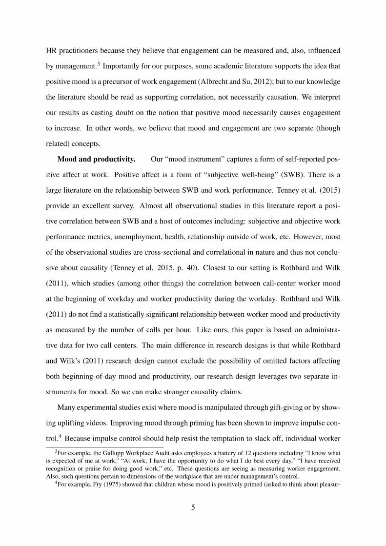
Mood is measured through an online “mood questionnaire” which the workers are encouraged

to fill out daily: see Figure 1.2 Productivity is measured by the number of calls per worker/hour,

1Gallup Inc. has measured workplace well-being for decades, and has long supported the notion of a linkbetween wellbeing and productivity. Jim Harter, Chief Scientist of Gallup’s Workplace Wellbeing Practices, writesthat “Investigation of the happy productive worker clearly links emotional well-being with job performance.”

2The mood questionnaire arises from the company’s desire to measure worker engagement.

2

Figure 1: Screenshot of Mood Questionnaire

and by other measures including downtime, time the customer is put on hold, and customer

satisfaction.

The panel structure of the data allows us to use worker fixed effects. Identification therefore

leverages within-worker variation in mood. Controlling for worker time-invariant characteris-

tics (like worker ability), we find that better mood is negatively correlated with productivity.

Though provocative, this finding is consistent with the experimental psychology literature on

distraction and sociability. But we seek causal effects. The call-center setting is especially suit-

able for our purposes because variation in call-center demand (a likely confounder of produc-

tivity) is national, and thus independent of local shocks to mood which can be used to estimate

the causal effect of mood.

We instrument for mood with local weather on the same day and, separately, with whether a

local professional sports team played the day before. The first-stage estimates are as expected:

rain worsens mood, and the local sports team playing improves mood (though the latter effect

is somewhat weak, perhaps due to some heterogeneity in the response: the male workers’ mood

improves mainly after wins). Using these two instruments we estimate that mood has a very siz-

able, and similarly-sized for both instruments, negative causal effect on our call-center workers’

productivity. Both IV estimates are much larger than the OLS estimates (direct effect of mood

on productivity). We provide direct evidence of a reverse-causation bias in the OLS estimates

that may partly account for this difference.

We find that the effect of mood is more muted for the subset of call-center workers whose

compensation depends on productivity (high-powered incentives). In other words, mood affects

productivity more so when incentives are low-powered. This finding is consistent with a possi-

3

ble distraction effect of mood: workers for whom getting distracted has a higher monetary cost

are less likely to do so when they are in a good mood. This may be interpreted as indicating

that introducing monetary incentives crowds out the impact of mood.

The causal interpretation of our estimates rests on the assumption that the effect of weather

or sports games on productivity is mediated by mood alone. A first concern is that demand

might be related to weather (and maybe also to sports events). However, our call centers face a

national demand: calls from all over the U.S. are first centrally directed then routed to individual

call centers; thus we are able to show that demand is uncorrelated with our instruments. A

second concern is that our instruments might affect the number of hours a worker shows up at

work (e.g., bad weather may increase traffic; sports events may increase the likelihood that a

worker shows up late); and this may affect productivity per hour. However, we show that the

results hold if we control for the “number of hours at work,” or if we replicate the analysis on

the subsample of workers who live close to the office. A third concern, which is specific to

our weather instrument, is that forecasted weather might require workers to waste productive

time rearranging their schedules (if rain is forecasted, cancel the BBQ, and vice versa). The

idea is that if rain is forecasted tomorrow, a worker might have to spend some time today in

order to rearrange her personal schedule. To assess the importance of this concern, we regress

productivity at time t−1 on rain at time t; but we find no effect.

The paper proceeds as follows: Section 2 discusses the related literature; Section 3 presents

statistics and explains our institutional context. Section 4 presents a conceptual framework.

Sections 5 and 6 identify the correlation and the causal effect of mood on productivity: OLS and

IV results, respectively, and discusses potential threat to the IV identification strategy. Section

7 concludes by discussing the external validity of our results.

2 Related Literature

Mood as a precursor of engagement. Worker engagement is defined as “a positive,

fulfilling, work-related state of mind that is characterized by vigor, dedication, and absorption”

(Bakker 2008). This state of mind is seen as desirable in workers. Engagement is important to

4

HR practitioners because they believe that engagement can be measured and, also, influenced

by management.3 Importantly for our purposes, some academic literature supports the idea that

positive mood is a precursor of work engagement (Albrecht and Su, 2012); but to our knowledge

the literature should be read as supporting correlation, not necessarily causation. We interpret

our results as casting doubt on the notion that positive mood necessarily causes engagement

to increase. In other words, we believe that mood and engagement are two separate (though

related) concepts.

Mood and productivity. Our “mood instrument” captures a form of self-reported pos-

itive affect at work. Positive affect is a form of “subjective well-being” (SWB). There is a

large literature on the relationship between SWB and work performance. Tenney et al. (2015)

provide an excellent survey. Almost all observational studies in this literature report a posi-

tive correlation between SWB and a host of outcomes including: subjective and objective work

performance metrics, unemployment, health, relationship outside of work, etc. However, most

of the observational studies are cross-sectional and correlational in nature and thus not conclu-

sive about causality (Tenney et al. 2015, p. 40). Closest to our setting is Rothbard and Wilk

(2011), which studies (among other things) the correlation between call-center worker mood

at the beginning of workday and worker productivity during the workday. Rothbard and Wilk

(2011) do not find a statistically significant relationship between worker mood and productivity

as measured by the number of calls per hour. Like ours, this paper is based on administra-

tive data for two call centers. The main difference in research designs is that while Rothbard

and Wilk’s (2011) research design cannot exclude the possibility of omitted factors affecting

both beginning-of-day mood and productivity, our research design leverages two separate in-

struments for mood. So we can make stronger causality claims.

Many experimental studies exist where mood is manipulated through gift-giving or by show-

ing uplifting videos. Improving mood through priming has been shown to improve impulse con-

trol.4 Because impulse control should help resist the temptation to slack off, individual worker

3For example, the Gallupp Workplace Audit asks employees a battery of 12 questions including “I know whatis expected of me at work,” “At work, I have the opportunity to do what I do best every day,” “I have receivedrecognition or praise for doing good work,” etc. These questions are seeing as measuring worker engagement.Also, such questions pertain to dimensions of the workplace that are under management’s control.

4For example, Fry (1975) showed that children whose mood is positively primed (asked to think about pleasur-

5

productivity is presumably improved by better mood.5 Overall, these experiments afford strong

causality claims, but collectively their findings are somewhat ambiguous with regards to pro-

ductivity, and it unclear how these findings extend to actual workplaces. In particular, these

experiments do not allow experimental subjects to have “social downtime” which they can sub-

stitute for work time, and so the effect of mood on this substitution cannot be observed.6

Mood and Sociability. Priming a better mood has been shown to increase the sub-

jects’ vulnerability to distractions (Pacheco-Unguetti & Parmentier 2016), and to increase socia-

bility (see Cunningham 1988 and the literature cited therein). Neither trait necessarily promotes

productivity “in the wild,” as shown in the next paragraph.

Sociability and Productivity. A number of papers study how socializing affects em-

ployee productivity. In the context of a seafood-processing plant in Vietnam in which worker

productivity is individual, Park (2016) shows that productivity declines by up to 9% when work-

ers have their friends nearby and socialize. In the context of call-center workers in China, Bloom

et al. (2014) show that workers who work from home are 13% more productive. The effect is at-

tributed, partly, to the relative quiet at home and, possibly, to the absence of socializing. Overall,

this literature suggests that in a number of work settings sociability decreases performance.

Summary of our contribution to the literature. In sum, the current research does

not study the causal effect of mood on individual productivity in the field. Our paper is the

first to address this question, and it does so through an instrumental variable strategy. A further

contribution of our paper is to demonstrate that mood affects productivity more strongly when

incentives are soft (fixed salary) than when they are hard (pay for performance).

able events) are better able to resist temptation (play with a forbidden toy) than children whose mood is neutral oris negatively primed. Fry’s early insight has since been validated in a many different settings. Inducing emotionaldistress has been shown to impair the ability to: moderate food consumption; stop smoking; stop gambling; avoidcompulsive shopping; and generally delay gratification. See Tice et al. (2001) for a review of this literature.

5This is the interpretation favored by Oswald et al. (2015), who shows that inducing happiness in experimentalsubjects by showing them humorous videos causes the subjects to perform long additions faster.

6Consistent with our reduced-form findings, Lee et al. (2014) find that bad weather increases individual pro-ductivity in three experimental designs and one field observational study, in a setting where productivity is notdirectly affected by weather. However, Lee et al. (2014) stop short of using weather as an instrument for mood.

6

3 Data and institutional setting

Our call-center data cover 2,749 workers located in 9 call centers across 9 different US states

from January 2015 to February 2016. 73% of call centers workers are females. They are 34

years of age on average and mean tenure is 39 months (see Table 1).

Each call center representative works in a cubicle with a computer and a headset. Whenever

a representative is ready to accept calls, she is asked to clock in to the IT system and calls

are automatically routed into her headset. A call from any location in the US is randomly

allocated to whichever worker in any of the locations happens to be available. To take a break,

a worker temporarily pauses the system. In this case she stops receiving calls and is logged as

not available to receive calls. At the end of the working day, the employee is asked to clock out

of the system.

These IT records provide us with detailed information on worker’s daily productivity (see

Table 1). For each worker, we know the number of hours she shows up at work (mean is 6.23)

and the proportion of these hours that are “unproductive” (i.e., downtime: off the phone and

unavailable to receive a call; mean is 10%). We also have information on the number of calls

per hour handled by each worker (mean is 6.9), average call duration (7.2 minutes per call on

average) and the proportion of time a customer is put “on hold” (14% on average). Finally, the

company provided us with information on average daily customer satisfaction (Likert scale 1-

10, average 8). Customer-reported productivity measures are available for relatively few calls;

this may be because few customers are selected to answer these questions, or because few

customers choose to answer them. In the latter case an issue of selection arises, but we have no

visibility of customers non-response, so we take these numbers at face value.

Workers are divided into two positions: customer service representative, and sales represen-

tatives. Customer service representatives have the role of providing information about products

and services, take orders, respond to customer complaints, and process returns. Sales represen-

tatives evaluate consumer needs, recommend and sell products. The two call-center positions

differ in the compensation scheme. Customer service representatives are paid a fixed hourly

rate (mean is 11.5 dollars) and earn almost no commission on top of that. Sales representatives

7

Table 1: Summary Statistics

VARIABLES Obs. Mean S.D.

A) Demographics and Position (N=Workers)=1 if Female 2,749 0.73 0.45Age 2,749 33.66 13.81Position= Customer Service Representative 2,749 0.54 0.50Position= Sales Representative 2,749 0.37 0.48Position= Other 2,749 0.09 0.28Tenure (in months) 2,736 38.62 59.71Distance from home to the office (in km) 2,723 15.43 11.57

B) Productivity (N=Workers*Days)No. calls per hour 219,279 6.90 8.10No. hours at work 219,279 6.23 1.96Proportion `unproductive' time 219,279 0.10 0.08Average call duration (in minutes) 219,277 7.19 4.98Proportion of call duration "on hold" 219,271 0.14 0.13No. customers answering customer survey 219,277 0.58 1.02

Average daily customer satisfaction (1 to 10)[Conditional on at least 1 answer] 74,513 8.00 2.54

C) Earnings (N=Workers*Months)Daily earnings (gross) Customer Service Representative 11,107 1123.03 513.65

2,571 1208.60 593.70 Sales Representative Daily earnings per hour (fixed + variable pay; gross) Customer Service Representative 11,072 11.82 1.05 Sales Representative 2,568 13.65 4.71Proportion of earnings that are "incentivized" (vs. fixed) Customer Service Representative 11,072 0.02 0.06 Sales Representative 2,568 0.42 0.51

Notes: All variables in Panel A correspond to the most recent observation of each worker (one observation per worker). Panel B displays the mean and standard deviation of daily-level productivity measures (one observation per day and per worker). No. calls per hour = total number of daily calls divided by total hours at work. Proportion `unproductive' time= % time not spent on the phone with customers or not spent being available to receive phone calls. Proportion of call duration "on hold" = % time the worker puts the customer on hold vs. talk to the customer. Customer satisfaction score calculates the average daily customer satisfaction score for each worker (score 1 to 10). This variable is missing if none of the customer were asked to fill the survey and/or none of the customers answered the survey. Panel C presents information on worker earnings for customer representatives and sales representatives separately, at the monthly level (data is available at the monthly level).

8

earn a lower fixed hourly salary (mean is 7.9 dollars) with commissions on top (5.7 dollars per

hour on average). While the incentive scheme differs across the two positions, the aggregate

month pay is similar (1123 vs. 1208 dollars respectively). Workers are also similar in terms of

tenure, age and gender. Neither position is segregated in specific call center locations.

For both positions, our preferred measure of productivity is the “number of calls per hour.”

(Productivity is recorded hourly, rather than “per day” or “per shift,” and workers are compen-

sated hourly in this firm.)7 As a measure of downtime, we also report “the proportion of time a

worker is unproductive (not available to receive calls)” and “the proportion of the call duration

which is on hold.” In Table A.1, we show that the raw correlation between these proxies of

downtime and the “number of calls per hour” is negative, while we find a positive correlation

between the number of calls handled per hour and average customer satisfaction.

Mood is measured through an online “mood questionnaire” which the workers are encour-

aged to fill out: see Figure 1 and Table 2. Individual answers are anonymous; each call center

manager is provided with monthly summary statistics aggregated at the call-center level. The

questionnaire is presented to the worker upon logging into a particular software platform and

is asked only once per day. Logging in is required to access a number of HR functions includ-

ing tracking their pay information, accessing online training, setting one’s quarterly goals, and

giving and receiving performance feedback. Accordingly, we assume that the login choice is

largely determined by considerations other than mood and we restrict our sample to the 77,514

worker-days in which the worker logged in the platform. We provide evidence in support of

the assumption in Table 7 (Column 1) where we show that our weather and sports instruments

(which are related to mood) have either a very small effect or no effect at all on the login choice.

Conditional on logging into the platform, a worker answers the mood question 46% of the

time, while skips the question – by pressing an “exit” button – the rest of the time (see Table 2).

This requires taking a stand on how to code non-responses. It is believed by HR managers in the

organization that non-response to the mood question is an indication of bad mood. In personal

communication with one HR manager, the authors learned that workers may be uneasy reporting

7We do not focus on the “number of hours an employee shows up at work” as a key outcome variable because:(1) workers are compensated hourly and (2) schedules are set by the firm a week in advance and are thus unaffectedby daily mood.

9

Table 2: Summary Statistics of Mood Question

VARIABLES Obs. Mean S.D.

Daily Worker Mood (N=Workers*Days)

=1 if worker logs into platform 219,279 0.35 0.48Conditional on logging into platform…

=1 if worker answers mood question 77,514 0.46 0.50

% who feel Frustrated 35,783 0.08 0.26% who feel Exhausted 35,783 0.07 0.25% who feel SoSo 35,783 0.17 0.38% who feel Good 35,783 0.35 0.48% who feel Unstoppable 35,783 0.33 0.47

35,783 3.80 1.19between-workers S.D= 1.02

within-worker S.D= 0.75

Conditional on answering Mood Question …

Notes: Upon logging into an online platform, workers are asked the mood question; "How do you feel today: Frustrated, Exhausted, So so, Good or Unstoppable?" The question is asked maximum one time per day. The worker has the option of answering the mood question or skipping it. We report here the mood score conditional on answering the mood question (coding the no answer as missing).

Mood score 1 to 5 [1= frustrated ... 5=unstoppable]

10

bad mood despite the organization’s assurance of anonymity of survey results. Consistent with

this view, “bad mood” is underreported (see below). Moreover, the percent of “no answers” is

lower on Fridays, when mood is believed to be higher (start of the weekend).

We report all results following two approaches and we show that the results are consistent

regardless of how the missing responses are coded. In the first approach, we assume that “no

answer” means “bad mood” (frustrated). In the second, we discount the selection concern and

code the non-responses as missing observations, thus effectively dropping non-responses and

halving the sample. We also show that our results are robust to imputing intermediate mood

scores for “no answer” in the appendix.8

Conditional on answering the mood question, 68% of respondents report feeling either

“good” or “unstoppable”, while only 15% report feeling “exhausted” or “frustrated.” Mood

score (which takes value 1 for “frustrated”, 2 for “exhausted, 3 for “so so”, 4 for “good” and 5

for “unstoppable”) takes an average value of 3.8 among the respondents. As a validation check

of our mood data, we correlate reported mood with “days of the week” in Table A.2. As one

would expect, mood is higher on Fridays and lower during weekends (consistent with the notion

that employees do not like to work during weekends). Importantly, the variation in mood score

exists both between workers (s.d. 1.01) and also within workers (s.d. 0.75). The within-worker

portion of the variation is sizable. Because we use worker fixed effects, identification will come

from within-worker variation: we compare the productivity of a given worker in days in which

she is in good mood to days in which she is not.

4 Conceptual framework

This section makes two conceptual points. First, it presents a micro-foundation that rationalizes

why a worker’s productivity might be decreasing in mood. The basic insight is that better mood

makes the worker more sociable, thus increasing the value of work (down)time spent socializing

relative to work time spent on solitary productive activities (refer to the literature on mood and

sociability discussed in Section 2). This effect might be stronger when the productive activity8 Reassuringly, our instruments do not affect the dispersion of the mood answer (available upon request), in

which case coding no answers as “bad mood” may be incorrect.

11

is solitary whereas downtime is social, as is the case in our call-center setting. Second, this

section studies a firm which may decide how much to invest in improving workplace mood

vs compensation. The firm chooses the optimal investment mix on mood and compensation

in order to maximize effort conditional on retaining the worker. Improving workplace mood

decreases effort, but it increases worker’s welfare, which helps the firm retain workers.

A worker allocates a unit of time (workday, e.g.) between effort e and downtime d. Com-

pensation is: a fixed salary W plus a piece-rate w. The worker’s problem is:

maxe,d

u (W +we)+ g (d,m)

s.t. e+ d = 1.

where u (·) is the (concave) utility from wealth, and g (·, ·) is the utility of downtime which is

assumed to be concave in d.

Substituting from the constraint into the utility function we get:

maxe

u (W +we)+ g (1− e,m) .

Let e∗ (W ,w,m) denote the solution to this problem.

Proposition 1. Fix the compensation scheme (W ,w) . Suppose g1,2 > 0, that is, every ad-

ditional unit of downtime is more valuable when mood is better. Then optimal effort

e∗ (W ,w,m) is decreasing in mood m.

Proof. Because of concavity, the first order conditions characterize optimal effort choice, and

so optimal effort e∗ solves:

(1) wu′ (W +we) = g1 (1− e,m) .

Because g1,2 > 0, increasing m to m′ raises the right hand side which, by concavity, is an in-

creasing function of e. Therefore the optimal e gets smaller.

12

This proposition rationalizes why a worker’s productivity might be decreasing in mood.

The proposition takes the compensation scheme as fixed, and it does not ask what optimal

compensation scheme might be put in place by a firm who can also, at a cost, affect workplace

mood. Next we sketch the problem of a firm which sets the compensation scheme and work-

place mood to maximize profits. Workplace mood can be manipulated in a variety of ways,

including: more time off, longer breaks, office celebrations and events, allowing the use of

social media at work, free food in the workplace, etc.

The firm’s problem is :

maxW ,w,m

(1−w)e∗ (W ,w,m)−W −K (m)(2)

s.t. U∗ (W ,w,m) ≥Ω

In this formulation K (m) represents the cost of creating mood m (we assume it is increasing

in m); the function U∗ represents the worker’s indirect utility function, that is, the worker’s

maximum attainable utility given (W ,w,m) ; and Ω represents the value of the worker’s outside

option, which is a measure of labor-market tightness. The reason why the firm might want to

incur a cost to increase mood is that mood improves U , and thus makes it easier to meet the

worker’s participation constraint.

In the appendix, we solve (2) within a specific functional-form example where: W ≡ 0,

that is, workers are paid a piece rate w; u (x) =√

x;g (d,m) = m√

d, and m ≥ 1. Given these

primitives we compute:

e∗ (w,m) =w

w+m2

U∗ (w,m) =√

w+m2.

We then show that if labor market tightness Ω2 is below√

2 then the participation constraint

in (2) is not binding. In this scenario the firm optimally chooses to make no investment in im-

proving mood, and the optimal piece rate is w∗ =√

2−1≈ 0.41. If the participation constraint

binds, i.e., labor market tightness Ω2 exceeds√

2, then the optimal piece rate w∗ > 1/2 and

13

the firm chooses to invest in improving mood. Finally, we show that as labor market tightness

grows above√

2 then the optimal piece rate w∗ grows. As for the optimal investment in mood,

it will grow or shrink with Ω depending on the functional form assumed for K. Therefore, in

general mood can be a complement or a substitute to the optimal piece rate as labor market

tightness grows.

5 Negative correlation between mood on productivity:

OLS results

Table 3 reports the correlation between mood and productivity in our sample of call-center

workers. As explained above, we have daily-level individual mood and productivity data. The

panel structure of the data allows us to include worker fixed effects, thus controlling for any

endogeneity that may arise across workers and is fixed through time. We also add date fixed

effects (day x month x year), and control for worker tenure.9 Standard errors are clustered

at the worker level and at the call-center*date level (two-way clustering). This accounts for

correlation within a given worker and across workers of a given call-center in a given day. In

the appendix Table A.3, we show that our results remain identical if we allow for autocorrelation

at short horizon by clustering standard errors at the call center*week level.

Regardless of how mood is coded, we find that a higher mood score is negatively correlated

with productivity: a one unit increase in mood decreases the number of calls per hour by 6pp

(Table 3, Column 1).10 The correlation is relatively linear across the different moods: the

highest the mood score, the lowest the number of calls per hour (see Table A.7). Finally, mood

is found to be positively correlated with call duration while the correlation with “the proportion

of unproductive time” and customer satisfaction is very small (at least in these OLS regressions).

While not causal, these results indicate that within-worker variation in mood is negatively

correlated with productivity (as measured as “calls per hour”) for call-center operators. Is this

negative correlation true in other work settings? We can answer this question for more than9We do not include workers’ position and call-center fixed effects as these are fixed within a worker (we do not

observe position or call-center switches).10See Table A.4 for alternative coding assumptions.

14

Table 3: Mood and Productivity, OLS Results

(1) (2) (3) (4) (5)

Dep. Var # calls per hour

% un- productive

time

Average call duration (minutes)

% of call duration "on hold"

Average customer

satisfaction (1 to 10)

Panel A: Conditional on answering Mood Question

Mood Score (1 to 5) -0.061*** -0.002*** 0.081*** -0.001 0.019(0.015) (0.001) (0.020) (0.001) (0.027)

Observations 33,461 33,461 33,461 33,461 14,725Rsquared 0.819 0.312 0.762 0.755 0.269Mean Dep Var 6.956 0.0981 7.866 0.150 8.140

Panel B: Assuming that not answering Mood Question = Bad Mood

Mood Score (1 to 5) -0.056*** -0.000 0.048*** -0.001 0.004(0.011) (0.000) (0.014) (0.001) (0.015)

Observations 73,268 73,268 73,268 73,268 32,305Rsquared 0.815 0.297 0.752 0.743 0.250Mean Dep Var 7 0.0960 7.719 0.151 8.049Worker FE Day x Month x year FE Notes: All regressions control for worker tenure. Standard errors are clustered (twoway) at worker & call center*date level. *** p<0.01, ** p<0.05, * p<0.1.

15

20,000 sales associates in more than 500 retail stores covering the entire US who used the same

online platform from September 2013 until August 2015.11 Unlike call-center workers, we can-

not link individual mood with individual performance, but we can link store-level productivity

(at the monthly level) with average store-level mood in that month. Controlling for store fixed

effects, month x year fixed effects and for the number of workers in the store, Table A.6 shows

that the correlation is negative: higher mood score is associated with lower average store profits

and revenues. This shows that the negative correlation observed among our call center workers

generalizes to a larger and more representative pool of workers.

A limitation of OLS estimates is that they are subject to potentially large endogeneity, re-

verse causality and strong measurement error. Because of these concerns, we turn to an IV

strategy in the next section. We focus on the call-center dataset as the store-level data are not

granular enough to perform any analysis beyond a simple OLS.12

6 Negative effect of mood on productivity: IV estimates

There are two reasons to believe that OLS estimates may underestimate the size of the effect of

mood on productivity. First, reverse causality: a worker who happens to be highly productive

on a given day may feel happier because of that. Table A.7 (Column 2) provides suggestive

evidence of a feedback effect of work environment on our mood variable. Workers who an-

swered the mood question were then asked a follow-up question: “What contributed the most

to your mood?” and could identify the source of their mood as work-related (“boss,” “work

environment,” “co-workers,” etc.); or “non-work related.” We believe that work-related mood

is more likely to be subject to reverse causality. Indeed, work-related mood turns out to be

positively correlated with productivity, whereas non-work-related mood is negatively correlated

(coefficient of -0.74). Therefore, there is reason to believe that OLS estimates are significantly

attenuated by reverse causality.

11The proportion of workers who answer the mood question conditional on logging in and the average moodscore among sales associates is very similar to the one of call-center workers, with a similar distribution of answers(see Table A.5)

12Productivity data are aggregated at the store level and does not vary at the daily level.

16

The second reason to believe that OLS estimates underestimate the impact of mood is clas-

sical measurement error in the mood variable. Mood is intrinsically hard to measure, especially

when captured through surveys.

Due to these concerns about downward bias of the OLS estimates, we now present IV esti-

mates based on two separate instruments for daily mood: daily weather and professional sports

events. Both instruments yields quantitatively similar estimates for the effect of mood.

6.1 First-stage results

Weather instrument. We use weather as an instrument for worker mood, because we expect

bad weather to cause worse mood. The existing literature offers support for this notion. Seasons

are known to affect mood: in some people, the winter months bring bad mood and depression

(seasonal affective disorder). Higher-frequency weather (daily, rather than seasonal) has also

been found to affect mood (Keller et al. 2005, Braga et al. 2014).13

The weather data come from the National Oceanic and Atmospheric Administration (Global

Historical Climatology Network-Daily Dataset). The data contain four weather variables at the

daily and zipcode levels: precipitation, maximum and minimum temperatures, and snowfalls.

As an instrument, we choose the weather variable that is found to be most positively correlated

with mood: whether it rains or not during the day, i.e., whether precipitations are strictly pos-

itive, which is known to correlate with sunshine. As shown in Table A.8, the “rain dummy”

negatively affects mood with an F-statistics of 16.25 when no response is coded as “bad mood,”

and of 9.4 when no response is coded as “missing.” Using all four weather variables as instru-

ments for mood, or using “rain precipitation” (in ml) alone leads to lower F-statistics and hence

we prioritize “rain dummy” as our instrument.

In our sample, 61% of the days were rainy with considerable variation across days (s.d.

0.49). Rain also varies across localities, but not enough to precisely estimate our coefficients

controlling for date fixed effects. In all specifications in which we use rain as our instrument

for mood, we control for: day-of-the-week fixed effects and month x year fixed effects. We

also control for the historic amount of rain in each calendar day (average in the past 5 years) to13Braga et al. (2014) show that on rainy days college students are harsher in their teaching evaluations.

17

further control for seasonality.

Professional sports games instrument. For each call center, we collected information on

whether the local sport team (football, baseball, basketball, or hockey) played on any given

day.14 As shown in Table A.8, employee mood is higher if the local team played the day before.

However, the first stage has limited power: statistical significance is only achieved in Panel B

(where no answer is coded as bad mood) and, even then, the F-statistic is relatively low (=6).

Despite this limitation we feel that this second instrument adds depth to our story, and so in

what follows, we will use this instrument in Panel B.15

6.2 Second-stage results

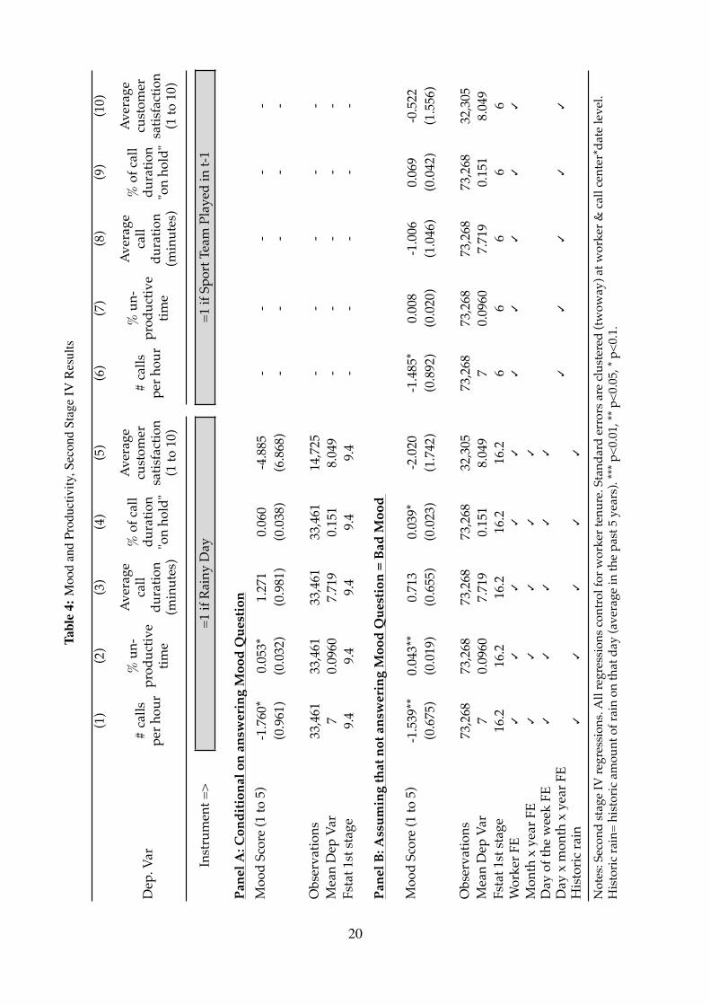
Our second-stage estimates are presented in Table 4. Regardless of how we code mood “no

answers,” we find that one unit increase in mood score reduces the “number of calls per hour”

by roughly 1.5, equal to 20% of the average. This result holds both with the rain and with the

sports instrument.

A reduction in the “number of calls handled per hour” can be explained by two possible

channels: either calls become longer or workers spend less of their time on the phone. Table

4 shows that both channels are at play. A one unit increase in the mood score increases the

proportion of “unproductive time” (downtime) by 4 to 5 percentage points depending on the

specification. This corresponds to a 50% increase in unproductive time. Call duration also

increases with mood, although not precisely and not in all specifications. This increase in

call duration is due to customers being kept on hold: the “percentage of minutes on hold”

increases by 4 to 6 percentage points, corresponding to a 40% increase relative to the average.

While “longer calls” and “more time on hold” may not necessarily reflect lower productivity

(but could reflect a higher willingness to help the client for instance), we find that customer

satisfaction scores decrease by up to 41% (though the coefficients are not significant due to the

14We use “whether a sports team played” rather than whether the team won or lost, because winning and losingappear to have similar first-stage effects (both positive) on mood. We were puzzled by this finding until we brokedown the first stage by gender. We found that, whereas for women good mood was associated with the teamplaying the day before irrespective of winning or losing, for men, the mood after a win was three times as high asafter a loss.

15Adding a second-stage weak instrument correction (LIML estimator) does not change the second-stage results.

18

small number of observations in which customer satisfaction is recorded). Moreover, the fact

that the proportion of “unproductive time” increases necessarily means that workers spend less

of their time effectively working.

Table A.9 presents the same results with alternative coding strategies. While the exact co-

efficients change from one coding strategy to another, the coefficients are consistently negative

and large in magnitude. Table A.11 shows that the results survive with standard errors clustered

at call-center*week level.

The overall picture, then, is one of fewer number of calls per hour, a reduction in “productive

working time” and an increase in the “proportion of time a customer is placed on hold.” Our

conclusion is that an exogenous increase in mood causes productivity to decline and this decline

seems to be explained by an increase in downtime.

We now introduce the distinction between customer service and sales representatives. The

former are almost entirely compensated by fixed compensation per hour worked. The latter

have a significant part of their compensation based on “sales per hour” and “number of calls

per hour.” In our sample, customer service representatives earn an average of 1,123 dollars

per month (gross), 98% of which comes from a fixed hourly pay. Sales representatives earn

slightly more: 1,209 dollars per month and 41% of these earnings is “variable” and based

on performance (see Table 1). Because sales positively correlate with the number of calls,

the organization evaluates workers in both positions with the same performance metrics: the

“number of calls per hour.”

Table 5 indicates that the effects of mood on productivity are weaker for the subsample of

sales representatives, in that the coefficients on the interaction term “Mood Score x Sales Rep-

resentative” has the opposite sign to the “Mood Score” variable. Using rain as an IV for mood,

it appears that the “number of calls per hour” is 20% less responsive to mood for sales represen-

tatives than customer representatives (Panel B). This result is stronger (although less precise)

when using sports as an instrument for mood: sales representatives as 43% less responsive to

mood. Similarly, the “% unproductive time” and “% call duration on hold” are roughly 30%

less responsive to mood for sales representatives than for customer representatives with the rain

instrument (with the sports instrument, the effect on the “% call duration on hold” becomes

19

Tabl

e4:

Moo

dan

dPr

oduc

tivity

,Sec

ond

Stag

eIV

Res

ults

(1)

(2)

(3)

(4)

(5)

(6)

(7)

(8)

(9)

(10)

Dep

. Var

# ca

lls

per h

our

% u

n-pr

oduc

tive

time

Aver

age

call

dura

tion

(min

utes

)

% o

f cal

l du

ratio

n "o

n ho

ld"

Aver

age

cust

omer

sa

tisfa

ctio

n (1

to 1

0)

# ca

lls

per h

our

% u

n-pr

oduc

tive

time

Aver

age

call

dura

tion

(min

utes

)

% o

f cal

l du

ratio

n "o

n ho

ld"

Aver

age

cust

omer

sa

tisfa

ctio

n (1

to 1

0)

Inst

rum

ent =

>

Pane

l A: C

ondi

tiona

l on

answ

erin

g M

ood

Que

stio

nM

ood

Scor

e (1

to 5

)-1

.760

*0.

053*

1.27

10.

060

-4.8

85-

--

--

(0.9

61)

(0.0

32)

(0.9

81)

(0.0

38)

(6.8

68)

--

--

-

Obs

erva

tions

33,4

6133

,461

33,4

6133

,461

14,7

25-

--

--

Mea

n D

ep V

ar7

0.09

607.

719

0.15

18.

049

--

--

-Fs

tat 1

st st

age

9.4

9.4

9.4

9.4

9.4

--

--

-

Pane

l B: A

ssum

ing

that

not

ans

wer

ing

Moo

d Q

uest

ion

= Ba

d M

ood

Moo

d Sc

ore

(1 to

5)

-1.5

39**

0.04

3**

0.71

30.

039*

-2.0

20-1

.485

*0.

008

-1.0

060.

069

-0.5

22(0

.675

)(0

.019

)(0

.655

)(0

.023

)(1

.742

)(0

.892

)(0

.020

)(1

.046

)(0

.042

)(1

.556

)

Obs

erva

tions

73,2

6873

,268

73,2

6873

,268

32,3

0573

,268

73,2

6873

,268

73,2

6832

,305

Mea

n D

ep V

ar7

0.09

607.

719

0.15

18.

049

70.

0960

7.71

90.

151

8.04

9Fs

tat 1

st st

age

16.2

16.2

16.2

16.2

16.2

66

66

6W

orke

r FE

Mon

th x

yea

r FE

D

ay o

f the

wee

k FE

D

ay x

mon

th x

yea

r FE

H

isto

ric ra

in

=1 if

Rai

ny D

ay=1

if S

port

Tea

m P

laye

d in

t-1

Not

es: S

econ

d st

age

IV re

gres

sion

s. A

ll re

gres

sion

s con

trol

for w

orke

r ten

ure.

Sta

ndar

d er

rors

are

clus

tere

d (tw

oway

) at w

orke

r & ca

ll ce

nter

*dat

e le

vel.

His

toric

rain

= hi

stor

ic a

mou

nt o

f rai

n on

that

day

(ave

rage

in th

e pa

st 5

yea

rs).

*** p

<0.0

1, **

p<0

.05,

* p<

0.1.

20

even stronger, while the effect on “% unproductive time” is less strong).

Overall we find that mood affects productivity more so when incentives are low-powered.

This finding is consistent with the model in Section 4 because in that model changing the

power of incentives will alter the worker’s relative return of allocating a unit of time to ef-

fort vs downwtime. Note, however, that other alternative stories cannot be ruled out here: e.g.,

sales representatives may react more to mood because they are different ‘types of workers’ (e.g.,

less distractable or more money-driven) rather than because their compensation scheme is more

steep.

6.3 Threats to the exclusion restrictions

The size of the IV estimates is consistent across the two instruments, and we have provided

supporting evidence that rationalizes why it is larger than the OLS estimates. Nevertheless,

threats to the exclusion restrictions can never be discounted. Therefore, in this section we

investigate different threats to the exclusion restriction.

Hours worked. A first potential concern is that the number of hours an employee shows

up at work might be affected by weather or by whether the sports team played the day before.

E.g., rain may increase traffic and reduce hours worked, or, alternatively, rain may increase

hours worked by shifting leisure into work (see Connolly 2008). Similarly watching a sports

game the night before, may increase the number of workers late at work the day after. A direct

effect of our instruments on hours worked may violate the exclusion restriction if working more

hours negatively affects productivity per hour.16 To alleviate this concern we first show that

the second-stage results do not change if we control for the number of hours an employee was

at work (see Table 6, Table A.11 for other outcome variables, and Table A.12 for alternative

codings for mood). Second, we show that our rain and sports instruments have no direct effect

on the number of hours at work (intensive margin) and no effect on the number of workers who

are present at work (extensive margin); see Table 7, Columns 3 and 5. Finally, we find that the

results hold if we restrict the sample to workers who live less than 5km from the workplace and

who are therefore less likely to be delayed by traffic in getting to work (Table A.13).16The raw correlation between these two variables is presented in Table A.1 and is negative.

21

Tabl

e5:

Moo

dan

dPr

oduc

tivity

byIn

cent

ive

Stru

ctur

e,Se

cond

Stag

eIV

Res

ults

(1)

(2)

(3)

(4)

(5)

(6)

(7)

(8)

(9)

(10)

Dep

. Var

# ca

lls p

er

hour

% u

n-pr

oduc

tive

time

Aver

age

call

dura

tion

(min

utes

)

% o

f cal

l du

ratio

n "o

n ho

ld"

Aver

age

cust

omer

sa

tisfa

ctio

n (1

to 1

0)

# ca

lls

per h

our

% u

n-pr

oduc

tive

time

Aver

age

call

dura

tion

(min

utes

)

% o

f cal

l du

ratio

n "o

n ho

ld"

Aver

age

cust

omer

sa

tisfa

ctio

n (1

to 1

0)

Inst

rum

ents

=>

Pane

l A: C

ondi

tiona

l on

answ

erin

g M

ood

Que

stio

n

Moo

d Sc

ore

(1 to

5)

-2.7

040.

026

2.46

4*0.

073*

-2.8

88(2

.342

)(0

.032

)(1

.306

)(0

.042

)(5

.103

)M

ood

Scor

e* S

ales

Rep

rese

ntat

ive

0.28

1-0

.011

**-0

.097

-0.0

14**

*0.

303

(0.3

48)

(0.0

04)

(0.1

42)

(0.0

05)

(0.2

96)

Obs

erva

tions

35,4

2535

,425

35,4

2435

,424

15,4

10p-

valu

e (M

ood

+ M

ood*

Sales

rep=

0)0.

246

0.60

70.

055

0.14

00.

594

Pane

l B: A

ssum

ing

that

not

ans

wer

ing

Moo

d Q

uest

ion

= Ba

d M

ood

Moo

d Sc

ore

(1 to

5)

-3.1

87**

*0.

033*

*1.

301*

*0.

042*

*-1

.569

-1.0

000.

008

-1.5

320.

044

0.85

2(0

.949

)(0

.015

)(0

.623

)(0

.019

)(1

.477

)(1

.225

)(0

.025

)(1

.275

)(0

.037

)(2

.107

)M

ood

Scor

e* S

ales

Rep

rese

ntat

ive

0.65

0**

-0.0

12**

*-0

.175

-0.0

23**

*0.

463

0.43

30.

003

-0.1

44-0

.040

***

0.56

0(0

.289

)(0

.004

)(0

.136

)(0

.004

)(0

.328

)(0

.346

)(0

.009

)(0

.472

)(0

.011

)(0

.501

)

Obs

erva

tions

77,2

6877

,268

77,2

6777

,265

33,7

5177

,268

77,2

6877

,267

77,2

6533

,751

p-va

lue (

Moo

d +

Moo

d*Sa

les re

p=0)

0.00

20.

109

0.03

90.

258

0.35

30.

680

0.70

90.

246

0.90

30.

559

Mea

n D

ep V

ar fo

r Sal

es R

ep8.

606

0.09

86.

065

0.04

08.

951

8.60

60.

098

6.06

50.

040

8.95

1M

ean

Dep

Var

for C

usto

mer

Rep

6.76

40.

088

7.97

80.

180

7.66

06.

764

0.08

87.

978

0.18

07.

660

Wor

ker F

E

M

onth

x y

ear F

E

Day

of t

he w

eek

FE

Day

x m

onth

x y

ear F

E

His

toric

rain

Rain

y D

ay &

Rai

ny D

ay*S

ales

Rep

rese

ntat

ive

Team

Pla

yed

& T

eam

Pla

yed*

Sale

s Rep

rese

ntat

ive

Not

es: S

econ

d st

age

IV re

gres

sion

s. A

ll re

gres

sion

s con

trol

for w

orke

r ten

ure.

Sta

ndar

d er

rors

are

clus

tere

d (tw

oway

) at w

orke

r & ca

ll ce

nter

*dat

e le

vel.

His

toric

rain

= hi

stor

ic a

mou

nt o

f rai

n on

that

day

(ave

rage

in th

e pa

st 5

yea

rs).

*** p

<0.0

1, **

p<0

.05,

* p<

0.1.

22

Table 6: Mood and Productivity, Second Stage IV Results with Extra Controls

(1) (2) (3) (4) (5) (6) (7) (8)

Instrument =>

Panel A: Conditional on answering Mood QuestionMood score (1 to 5) -1.785* -1.743* -1.605* -1.546 -1.308

(0.964) (0.937) (0.929) (0.968) (1.087)No. hours at work -0.099*** -0.097*** -0.097*** -0.094***

(0.020) (0.020) (0.020) (0.024)No. incoming calls in call-center 0.043*** 0.043*** 0.046***

(0.014) (0.014) (0.015)Temperature -0.000 0.000

(0.000) (0.001)Nitric oxide (value) [Air pollution] 2.428

(3.063)Nitrogen dioxide (value) [Air pollution] 0.005

(0.003)Ozone (value) [Air pollution] -0.001

(0.005)

Observations 33,461 33,461 33,461 33,461 21,101Fstat 1st stage 0.658 0.667 0.690 0.700 0.727

Panel B: Assuming that not answering Mood Question = Bad Mood

Mood score (1 to 5) -1.542** -1.530** -1.439** -1.430** -1.344** -1.485* -1.480* -1.371(0.666) (0.653) (0.640) (0.633) (0.641) (0.892) (0.888) (0.863)

No. hours at work -0.084*** -0.084*** -0.084*** -0.086*** -0.059*** -0.059***(0.017) (0.016) (0.016) (0.021) (0.012) (0.011)

No. incoming calls in call-center 0.044*** 0.044*** 0.052*** 0.029**(0.012) (0.012) (0.014) (0.013)

Temperature -0.000 0.001(0.000) (0.000)

Nitric oxide (value) [Air pollution] 1.478(2.273)

Nitrogen dioxide (value) [Air pollution] 0.003(0.003)

Ozone (value) [Air pollution] -0.007(0.004)

Observations 73,268 73,268 73,268 73,268 46,761 73,268 73,268 73,268Fstat 1st stage 16.25 16.25 16.25 16.25 16.25 16.25 16.25 16.25Mean Dep Var 7 7 7 7 7 7 7 7Worker FE Month x year FE Day of the week FE Day x month x year FE Historic rain

Dependent variable = # calls per hour

Notes: Second stage IV regressions. All regressions control for worker tenure. Standard errors are clustered (twoway) at worker & call center*date level. Historic rain= historic amount of rain on that day (average in the past 5 years). *** p<0.01, ** p<0.05, * p<0.1.

=1 if Rainy Day =1 if Sport Team Played in t-1

23

Tabl

e7:

The

Red

uced

-For

mE

ffec

tson

Log

ging

-in,

Moo

dA

nsw

er,D

eman

dan

dPr

oduc

tivity

(1)

(2)

(3)

(4)

(5)

(6)

(7)

(8)

(9)

=1 if

logs

in

the

plat

form

=1 if

an

swer

s m

ood

ques

tion

# ho

urs a

t w

ork

# da

ily

inco

min

g ca

lls(in

'000

)

# w

orke

rs

pres

ent

at w

ork

=1 if

Rai

ny D

ay0.

006*

-0.0

01-0

.010

0.14

21.

916

0.05

1**

0.06

2**

(0.0

04)

(0.0

02)

(0.0

16)

(0.0

96)

(1.5

91)

(0.0

23)

(0.0

26)

0.03

00.

018

(0.0

20)

(0.0

23)

Wor

ker F

E

Mon

th x

yea

r FE

D

ay o

f the

wee

k FE

H

isto

ric ra

in

Spor

t Tea

m P

laye

d in

t-1

0.00

00.

005

-0.0

26-0

.023

-1.7

70-0

.035

-0.0

44(0

.005

)(0

.003

)(0

.018

)(0

.138

)(2

.596

)(0

.027

)(0

.000

)

Wor

ker F

E

Day

x m

onth

x y

ear F

E

Obs

erva

tions

214,

094

214,

094

214,

094

1,59

81,

598

214,

094

211,

371

75,9

4075

,148

R-sq

uare

d0.

457

0.45

00.

311

0.90

30.

892

0.79

50.

796

0.80

70.

808

Mea

n D

ep V

ar0.

354

0.16

37.

381

8.53

013

7.2

6.78

76.

787

77

Lead

Rai

n D

umm

y (=

1 if

Rain

y D

ay in

t+1)

Not

es: W

orke

r-le

vel r

egre

ssio

ns co

ntro

l for

wor

ker t

enur

e, w

ith st

anda

rd e

rror

s clu

ster

ed (t

wow

ay) a

t wor

ker &

call

cent

er*d

ate

leve

l. C

all-

cent

er le

vel r

egre

ssio

ns a

re co

llaps

ed a

t the

call

cent

er le

vel a

nd p

rese

nt st

anda

rd e

rror

s clu

ster

ed a

t the

call

cent

er*d

ate

leve

l. #

daily

in

com

ing

calls

(in

'000

) = th

e to

tal n

umbe

r of c

alls

rece

ived

in th

e ca

ll ce

nter

in a

giv

en d

ay. "

Lead

rain

dum

my"

=1

if it

rain

ed in

day

t+1.

H

isto

ric ra

in=

hist

oric

am

ount

of r

ain

on th

at d

ay (a

vera

ge in

the

past

5 y

ears

). Th

e nu

mbe

r of o

bser

vatio

ns is

hig

her i

n th

e fir

st 3

cols

than

in

the

prev

ious

regr

essi

ons b

ecau

se w

e do

*not

* res

tric

t the

ana

lysi

s on

wor

kers

who

logg

ed in

the

plat

form

in a

giv

en d

ay b

ut o

n al

l w

orke

rs (w

heth

er th

ey lo

gged

in o

r not

). **

* p<0

.01,

** p

<0.0

5, *

p<0.

1.

Wor

ker-

leve

l reg

ress

ions

C

all c

ente

r-le

vel

regr

essi

ons

Wor

ker-

leve

l reg

ress

ions

# ca

lls p

er h

our

# ca

lls p

er h

our

(Con

ditio

nal o

n Lo

ggin

g in

)

24

Demand. A second potential concern is that demand might be correlated with local weather,

as would be the case for a number of jobs (farmers, taxi drivers, physical sales positions).

Similarly, demand may be higher or lower the day after a local sports team plays. In our setting

(call centers), the demand our workers face is national, as calls from all over North America

are first aggregated and then distributed across call centers. Accordingly, we see that “number

of calls incoming to a call center” is uncorrelated with weather in that call center or with local

sports games the day before (Table 7 Column 3). The absence of confounding variation from

the demand side is a key advantage of a call-center setting. Finally, Table 6 (Column 3) shows

that the results do not change if we control for the “number of calls incoming.”

Pollution. A third potential concern is pollution. Pollution has been shown to reduce worker

productivity in call-center settings (Chang et al. 2016) and may correlate with rain. In Table

6, we show that the results hold if we control for temperature (which is related with daily

pollution) and for the level of three air pollutants (Nitric Oxide, Nitrogen Dioxide, and Ozone).

Unfortunately, the data are missing for one third of the sample and the sample size is therefore

smaller. Note that pollution is unlikely to be a confounder for our sports instrument.

Others. A final set of potential concerns (for the rain instrument only) is that rain might

have a direct effect on call-center working conditions independent of mood. Two possibilities

come to mind. First, that weather might affect productivity through distraction-on-the-job, i.e,

by looking out a window. Second, that forecasted weather might require changes in the work-

ers’ personal schedules, causing workers to waste time on the job rearranging their schedules (if

rain is forecasted, cancel the BBQ, and vice versa). To guard against the first concern, we have

obtained information about the prevalence of windows in different call center locations. Based

on our information, one third of the call centers have no windows at all while in the others all

workers see natural light. We check in Table A.14 whether workers in the call centers without

windows are less sensitive to rain-induced changes in mood (controlling for worker fixed ef-

fects). We find no significant effect. This indicates that the effect of mood on productivity may

not be affected by the presence of a window in the workplace, and suggests that the effect of

weather on mood is fully achieved in the time spent outside prior to reaching the workplace.17

17Table A.15 shows that the mood of workers without a window reacts to rain as much as the mood of workers

25

Note that the interaction terms in Table A.14 have large standard errors and that this evidence

is thus more suggestive than conclusive.

To assess the importance of the second concern (effect of forecasted weather), we regress

productivity at time t− 1 on rain at time t (which we call “lead rain.”) The idea is that if rain

is forecasted tomorrow, a worker might have to spend some time today in order to rearrange

her personal schedule. Table 7 Columns 6-9 show that the coefficient for “lead rain” is smaller

than the one for “contemporary rain” (roughly half of the magnitude) and is not statistically

significant. The effect of rain which we measure is thus likely not mediated by rescheduling. In

contrast, rain at time t significantly increases the number of calls per productive hour at t by 6.2

percentage points (reduced form).

7 Conclusions

A causal link between good mood and productivity, if established, would have profound con-

sequences for economic theory and for business practice. In this paper we make some initial

progress toward exploring this important link.

Conceptually, we provide a micro-foundation arguing that a worker’s productivity might be

decreasing in mood if better mood makes the worker more sociable, thus increasing the value

of work time spent socializing rather than working. Knowing whether, and how much, mood

decreases productivity is important for firms. Firms, we argue, routinely choose how much to

invest on workplace mood (by allowing more time off, longer breaks, office celebrations and

events, use of social media at work, etc) and in compensation, in order to maximize effort con-

ditional on retaining the worker. Improving workplace mood decreases effort, but it increases

worker’s welfare, which helps the firm retain workers. Thus knowing the effect of mood on

productivity may help the firm calibrate its compensation scheme.

At the correlational level, we present some of the first large-scale evidence of a correla-

tion between mood and productivity, with evidence coming from teams of sales representatives

from a large retailer, and also, separately, from individual-level data from call center work-

with a window.

26

ers. Provocatively, but consistent with some of the experimental psychology, this correlation is

negative.

We then leverage the call-center dataset to explore the causal effect of mood on their pro-

ductivity in the field through an IV strategy. The call center dataset is ideal to investigate the

causal effect of mood because variation in demand (a likely confounder of productivity) is na-

tional, and thus independent of our instruments – rain and sports events the day before. We find

that better mood actually decreases our call-center workers’ productivity. The effect of mood

is more muted for the subset of call-center workers whose compensation depends on produc-

tivity (high-powered incentives). This finding may be interpreted as indicating that introducing

monetary incentives crowds out the impact of mood.

We have ruled out a number of threats to the exclusion restriction: that our instruments

might affect productivity through higher demand, lower pollution, more hours at work, or more

time spent rearranging the workers’ personal schedules.

A number of caveats are in order. Our results concern short-term and individual mood

shifters only. In addition, we do not study worker retention empirically. Despite these limi-

tations, our research suggests that there are good theoretical reasons to believe that improving

workplace mood (by allowing more time off, longer breaks, etc.) entails some trade-offs, and

our empirical estimates have quantified the trade-off with productivity. It is quite possible that

firms have actually evaluated these trade-offs in setting compensation policy. So it may be

appropriate for the literatures in economics and management to include workplace mood as a

variable in the design of incentive schemes.

Finally, our findings relate to a specific workplace environment: call centers. The effects

of pro-sociality, which is our presumed operative channel, may impact differently depending

on how work is organized, e.g., whether the production function is individual, and if not, how

much teamwork there is.

27

References

[1] Bakker, Arnold B., et al. “Work engagement: An emerging concept in occupational health

psychology.” Work and Stress 22.3 (2008): 187-200.

[2] Bloom, Nicholas, et al. “Does working from home work? Evidence from a Chinese exper-

iment.” The Quarterly Journal of Economics 130.1 (2014): 165-218.

[3] Braga, Michela, Marco Paccagnella, and Michele Pellizzari. “Evaluating students’ evalua-

tions of professors.” Economics of Education Review 41 (2014): 71-88.

[4] Chang, T., Zivin, J. G., Gross, T., and Neidell, M. “The effect of pollution on worker

productivity: evidence from call-center workers in China”. American Economic Journal:

Applied Economics, forthcoming (2016)

[5] Connolly, Marie. “Here comes the rain again: Weather and the intertemporal substitution

of leisure.” Journal of Labor Economics 26.1 (2008): 73-100.

[6] Fry, Prem S. ”Affect and resistance to temptation.” Developmental psychology 11.4 (1975):

466.

[7] Keller, Matthew C., et al. “A warm heart and a clear head: The contingent effects of weather

on mood and cognition.” Psychological science 16.9 (2005): 724-731.

[8] Lee, Jooa Julia, Francesca Gino, and Bradley R. Staats. “Rainmakers: Why bad weather

means good productivity.” Journal of Applied Psychology 99.3 (2014): 504.

[9] Oswald, Andrew J., Eugenio Proto, and Daniel Sgroi. “Happiness and productivity.” Journal

of Labor Economics 33.4 (2015): 789-822.

[10] Pacheco-Unguetti, Antonia Pilar, and Fabrice BR Parmentier. “Happiness increases dis-

traction by auditory deviant stimuli.” British Journal of Psychology 107.3 (2016): 419-433.

Cunningham, Michael R. “What do you do when you’re happy or blue? Mood, expectan-

cies, and behavioral interest.” Motivation and emotion 12.4 (1988): 309-331.

28

[11] Park, Sangyoon. “Socializing at work: Evidence from a field experiment with manufac-

turing workers.” Mimeo (2016).

[12] Rothbard, Nancy P., and Steffanie L. Wilk. “Waking up on the right or wrong side of the

bed: Start-of-workday mood, work events, employee affect, and performance.” Academy

of Management Journal 54.5 (2011): 959-980.

[13] Tenney, E., J. Poole, and E. Diener. “Subjective well-being and organizational perfor-

mance.” Research in organizational behavior (2015).

[14] Tice, Dianne M., Ellen Bratslavsky, and Roy F. Baumeister. “Emotional distress regulation

takes precedence over impulse control: If you feel bad, do it!.” Journal of personality and

social psychology 80.1 (2001): 53.

29

A Tables and figures

Table A.1: Correlations between Productivity Measures

# calls per hour

# hours at work

% unprod-uctive time

Average call

duration

% of call duration "on hold"

# calls per hour 1# hours at work -0.0676* 1% unproductive time -0.0276* -0.0639* 1Average call duration -0.2182* 0.0410* 0.1275* 1% of call duration "on hold" -0.0607* 0.0027 0.1644* 0.2117* 1Average customer satisfaction 0.0656* -0.0126* -0.0344* -0.1614* -0.1791*Notes: Simple pairwise correlations. *p-value<0.05. N=Workers*Days

Table A.2: Mood and Days of the Week

(1) (2)

=1 if Weekend -0.041***(0.013)

=1 if Monday 0.043**(0.021)

=1 if Tuesday 0.040*(0.022)

=1 if Wednesday 0.034*(0.020)

=1 if Thursday 0.034(0.021)

=1 if Friday 0.068***(0.021)

=1 if Saturday 0.004(0.023)

Observations 35,425 35,425Rsquared 0.597 0.597Mean Dep Var 3.798 3.798Worker FE Month x year FE

Mood Score (1 to 5) [conditional on answering mood

question]

Notes: All regressions control for worker tenure. Robust standard errors clustered (twoway) at worker & call center*date level are presented in parenthesis. *** p<0.01, ** p<0.05, * p<0.1.

1

Tabl

eA

.3:M

ood

and

Prod

uctiv

ity,O

LS

Res

ults

with

Alte

rnat

ive

Clu

ster

ing

Stan

dard

err

ors

are

clus

tere

d (tw

oway

) at w

orke

r & c

all c

ente

r*w

eek

leve

l(1

)(2

)(3

)(4

)(5

)

Dep

. Var

# ca

lls p

er

hour

% un-

productive

time

Aver

age

call

dura

tion

(min

utes

)

% o

f cal

l du

ratio

n "o

n ho

ld"

Aver

age

cust

omer

sa

tisfa

ctio

n (1

to 1

0)

Pane

l A: C

ondi

tiona

l on

answ

erin

g M

ood

Que

stio

n

Moo

d Sc

ore

(1 to

5)

-0.0

61**

*-0

.002

***

0.08

1***

-0.0

010.

019

(0.0

15)

(0.0

01)

(0.0

19)

(0.0

01)

(0.0

28)

Obs

erva

tions

33,4

6133

,461

33,4

6133

,461

14,7

25Rs

quar

ed0.

819

0.31

20.

762

0.75

50.

269

Mea

n D

ep V

ar6.

956

0.09

817.

866

0.15

08.

140

Pane

l B: A

ssum

ing

that

not

ans

wer

ing

Moo

d Q

uest

ion

= Ba

d M

ood

Moo

d Sc

ore

(1 to

5)

-0.0

56**

*-0

.000

0.04

8***

-0.0

010.

004

(0.0

11)

(0.0

00)

(0.0

14)

(0.0

01)

(0.0

16)

Obs

erva

tions

73,2

6873

,268

73,2

6873

,268

32,3

05Rs

quar

ed0.

815

0.29

70.

752

0.74

30.

250

Mea

n D

ep V

ar7

0.09

607.

719

0.15

18.

049

Wor

ker F

E

Day

x M

onth

x y

ear F

E

Not

es:

All

regr

essi

ons c

ontr

ol fo

r wor

ker t

enur

e. S

tand

ard

erro

rs a

re cl

uste

red

(twow

ay) a

t w

orke

r & ca

ll ce

nter

*wee

k le

vel.

*** p

<0.0

1, **

p<0

.05,

* p<

0.1.

2

Tabl

eA

.4:M

ood

and

Prod

uctiv

ity,O

LS

Res

ults

with

Alte

rnat

ive

Cod

ing

(1)

(2)

(3)

(4)

(5)

Dep

. Var

# ca

lls p

er

hour

% u

n-pr

oduc

tive

time

Aver

age

call

dura

tion

(min

utes

)

% o

f cal

l du

ratio

n "o

n ho

ld"

Aver

age

cust

omer

sa

tisfa

ctio

n (1

to 1

0)

Pane

l C: A

ssum

ing

that

not

ans

wer

ing

Moo

d Q

uest

ion

= Ba

d M

ood

[Exh

aust

ed]

Moo

d Sc

ore

(1 to

5)

-0.0

71**

*-0

.000

0.06

4***

-0.0

010.

007

(0.0

13)

(0.0

00)

(0.0

16)

(0.0

01)

(0.0

19)

Pane

l D: A

ssum

ing

that

not

ans

wer

ing

Moo

d Q

uest

ion

= N

eutr

al M

ood

[So-

so]

Moo

d Sc

ore

(1 to

5)

-0.0

79**

*-0

.001

**0.

077*

**-0

.001

*0.

011

(0.0

15)

(0.0

00)

(0.0

18)

(0.0

01)

(0.0

23)

Obs

erva

tions

73,2

6873

,268

73,2

6873

,268

32,3

05M

ean

Dep

Var

70.

0960

7.71

90.

151

8.04

9W

orke

r FE

D

ay x

mon

th x

yea

r FE

N

otes

: A

ll re

gres

sion

s con

trol

for w

orke

r ten

ure.

Sta

ndar

d er

rors

are

clus

tere

d (tw

oway

) at

wor

ker &

call

cent

er*d

ate

leve

l. **

* p<0

.01,

** p

<0.0

5, *

p<0.

1.

3

Tabl

eA

.5:S

umm

ary

Stat

istic

sof

Moo

dQ

uest

ion

fort

he“S

tore

sD

atas

et”

VAR

IABL

ES O

bs.

Mea

nS.

D.

Dai

ly W

orke

r Moo

d (N

=Wor

kers

*Day

s)

Cond

ition

al o

n lo

ggin

g in

to p

latfo

rm…

=1 if

wor

ker a

nsw

ers m

ood

ques

tion

20,1

66,0

18

0.52

0.50

Cond

ition

al o

n an

swer

ing

Moo

d Q

uest

ion

…%

who

feel

Fru

stra

ted

10,4

86,3

29

0.06

0.17

% w

ho fe

el E

xhau

sted

10,4

86,3

29

0.06

0.17

% w

ho fe

el S

oSo

10,4

86,3

29

0.12

0.24

% w

ho fe

el G

ood

10,4

86,3

29

0.38

0.40

% w

ho fe

el U

nsto

ppab

le10

,486

,329

0.

390.

40

10,4

86,3

29

3.99

1.11

Moo

d sc

ore

1 to

5

[1=

frus

trat

ed ..

. 5=u

nsto

ppab

le]

Not

es: U

pon

logg

ing

into

an

onlin

e pl

atfo

rm, w

orke

rs a

re a

sked

the

moo

d qu

estio

n;

"How

do

you

feel

toda

y: F

rust

rate

d, E

xhau

sted

, So

so, G

ood

or U

nsto

ppab

le?"

The

qu

estio

n is

ask

ed m

axim

um o

ne ti

me

per d

ay. T

he w

orke

r has

the

optio

n of

an

swer

ing

the

moo

d qu

estio

n or

skip

ping

it. W

e re

port

her

e th

e m

ood

scor

e co

nditi

onal

on

logg

ing

into

the

plat

form

and

ans

wer

ing

the

moo

d qu

estio

n (c

odin

g th

e no

ans

wer

as m

issi

ng).

Stor

es D

atas

et

4

Tabl

eA

.6:M

ood

and

Prod

uctiv

ity,O

LS

Res

ults

fort

he“S

tore

sD

atas

et”

(1)

(2)

(3)

(4)

(5)

(6)

[All

valu

es in

Col

1-6

are

in

00,

000

USD

] =>

Reve

nues

G

ross

m

argi

n Eb

itda

Reve

nues

pe

r Em

ploy

ee-

Hou

r

Gro

ss

Mar

gin

per

Empl

oyee

-H

our

Ebitd

a pe

r Em

ploy

ee-

Hou

r

-0.3

18**

*-0

.119

***

-0.0

58**

-0.0

61**

*-0

.025

***

-0.0

08(0

.075

)(0

.030

)(0

.026

)(0

.018

)(0

.006

)(0

.005

)

Obs

erva

tions

17,4

0717

,407

17,4

0717

,407

17,4

0717

,407

R-sq

uare

d0.

933

0.89

80.

632

0.83

40.

733

0.52

5M

ean

Dep

Var

Stor

e FE

Mon

th x

yea

r FE

Not

es: T

he o

utco

me

varia

bles

var

y at

the

stor

e * m

onth

leve

l. A

ll re

gres

sion

s con

trol

for t

he to

tal

num

ber o

f wor

kers

in th

e st

ore.

Rob

ust s

tand

ard

erro

rs cl

uste

red

at st

ore*

date

leve

l are

pre

sent

ed in

pa

rent

hesi

s. **

* p<0

.01,

** p

<0.0

5, *

p<0.

1. A

vera

ge m

ood

scor

e =a

vera

ge m

ood

in a

stor

e-m

onth

acr

oss

wor

kers

who

ans

wer

ed th

e m

ood

ques

tion.

'Gro

ss m

argi

ns' i

s sto

re re

venu

e m

inus

cost

of g

oods

sold

. 'E

bitd

a' is

stor

e's e

arni

ngs b

efor

e in

tere

st, t

axes

, dep

reci

atio

n an

d am

ortiz

atio

n fo

r the

mon

th. '

Reve

nue

per E

mpl

oyee

*Hou

r' is

Tot

.Rev

. div

ided

by

the

sum

of a

ll em

ploy

ee h

ours

. 'Eb

itda

per p

er

Empl

oyee

*Hou

r' is

Ebi

tda

divi

ded

by th

e su

m o

f all

empl

oyee

hou

rs.

Aver

age

Empl

oyee

M

ood

Scor

e (1

to 5

)

Hid

den

for a

nony

mity

reas

ons

5

Tabl

eA

.7:M

ood

and

Prod

uctiv

ity,O

LS

Res

ults

byM

ood

(1)

(2)

Ass

umpt

ion

on M

ood

Que

stio

n =>

Moo

d by

moo

d w

ith

"no

answ

er"

as

omitt

ed g

roup

Cond

ition

al o

n an

swer

ing

Moo

d Q

uest

ion

&

answ

erin

g Re

ason

0.12

8(0

.082

)-0

.006

(0.0

58)

-0.0

96*

(0.0

54)

-0.1

08*

(0.0

55)

-0.2

39**

*(0

.051

)

0.05

4***

(0.0

16)

-0.7

39**

*(0

.167

)

Obs

erva

tions

34,1

8831

,709

Mea

n D

epen

dent

Var

iabl

e7

7W

orke

r FE

Day

x m

onth

x y

ear F

E

Dep

ende

nt v

aria

ble

= #

calls

per

hou

r

Not

es:

All

regr

essi

ons c

ontr

ol fo

r wor

ker t

enur

e. S

tand

ard

erro

rs a

re cl

uste

red

(twow

ay) a

t wor

ker &

call

cent

er*d

ate

leve

l. **

* p<0

.01,

** p

<0.0

5, *

p<0.

1.

=1 if

Moo

d=Fr

ustr

ated

(sco

re 5

)

=1 if

Moo

d=Ex

haus

ted

(sco

re 4

)

=1 if

Moo

d=So

so (s

core

3)

=1 if

Moo

d=G

ood

(sco

re 2

)

=1 if

Moo

d=U

nsto

ppab

le (s

core

1)

Moo

d sc

ore

if m

ain

reas

on e

xpla

inin

g th

e m

ood

is W

ork-

rela

ted

Moo

d sc

ore

if m

ain

reas

on e

xpla

inin

g th

e m

ood

is n

ot W

ork-

rela

ted

6

Tabl

eA

.8:M

ood

and

Wea

ther

/Spo

rtga

mes

;Fir

stSt

age

Res

ults

(1)

(2)

(3)

(4)

(5)

(6)

(7)

(8)

=1 if

Rai

ny D

ay-0

.031

***

-0.0

38**

*(0

.010

)(0

.009

)Pr

ecip

itatio

n-0

.001

***-

0.00

1***

-0.0

01**

*-0.

001*

**(0

.000

)(0

.000

)(0

.000

)(0

.000

)Sn

owfa

ll-0

.001

0.00

0(0

.001

)(0

.001

)M

inim

um te

mpe

ratu

re0.

001

-0.0

02(0

.002

)(0

.002

)M

axim

um te

mpe

ratu

re0.

001

0.00

1(0

.001

)(0

.001

)0.

008

0.04

2**

(0.0

15)

(0.0

17)

Fsta

t 1st

sta

ge9.

393

8.53

73.

002

0.28

016

.25

8.94

14.

497

5.95

7

Obs

erva

tions

33,4

6133

,461

33,4

6133

,525

73,2

6873

,268

73,2

6873

,341

R-sq

uare

d0.

599

0.59

90.

600

0.60

30.

684

0.68

40.

684

0.68

6M

ean

Dep

Var

3.80

13.

801

3.80

13.

801

2.28

92.

289

2.28

92.

289

Wor

ker F

E

M

onth

x y

ear F

E

D

ay o

f the

wee

k FE

Day

x m

onth

x y

ear F

E

H

isto

ric ra

in

Dep

ende

nt v

aria

ble

=Moo

d sc

ore

(1 to

5)

Pane

l A: C

ondi

tiona

l on

answ

erin

g M

ood

Que

stio

n

Pane

l B: A

ssum

ing

that

not

an

swer

ing

Moo

d Q

uest

ion

= Ba

d M

ood

Not

es: F

irst s

tage

IV re

gres

sion

s. A

ll re

gres

sion

s con

trol

for w

orke

r ten

ure.

Sta

ndar

d er

rors

are

clus

tere

d (tw

oway

) at w

orke

r & ca

ll ce

nter

*dat

e le

vel.

His

toric

rain

= hi

stor

ic a

mou

nt o

f rai

n on

that

day

(ave

rage

in

the

past

5 y

ears

). **

* p<0

.01,

** p

<0.0

5, *

p<0.

1.

=1 if

Spo

rt T

eam

Pla

yed

in t-

1

7

Tabl

eA

.9:M

ood

and

Prod

uctiv

ity,I

VR

esul

tsw

ithA

ltern

ativ

eC

odin

g

(1)

(2)

(3)

(4)

(5)

(6)

(7)

(8)

(9)

(10)

Asu

mpt

ion

on m

ood

ques

tion

=>

Dep

. Var

# ca

lls p

er

hour

% u

n-pr

oduc

tive

time

Aver

age

call

dura

tion

(min

utes

)

% o

f cal

l du

ratio

n "o

n ho

ld"

Aver

age

cust

omer

sa

tisfa

ctio

n (1

to 1

0)

# ca

lls p

er

hour

% u

n-pr

oduc

tive

time

Aver

age

call

dura

tion

(min

utes

)

% o

f cal

l du

ratio

n "o

n ho

ld"

Aver

age

cust

omer

sa

tisfa

ctio

n (1

to 1

0)

Moo

d Sc

ore

(1 to

5)

-1.9

33**

0.05

3**

0.89

60.

049*

-2.5

56-2

.598

**0.

072*

*1.

204

0.06

5*-3

.479

(0.8

36)

(0.0

24)

(0.8

17)

(0.0

29)

(2.1

95)

(1.1

35)

(0.0

34)

(1.0

93)

(0.0

39)

(3.1

14)

Obs

erva

tions

73,2

6873

,268

73,2

6873

,268

32,3

0573

,268

73,2

6873

,268

73,2

6832

,305

Mea

n D

epen

dent

Var

iabl

e7

0.09

607.

719

0.15

18.

049

70.

0960

7.71

90.

151

8.04

9Fs

tat 1

st st

age

17.1

217

.12

17.1

217

.12

17.1

215

.08

15.0

815

.08

15.0

815

.08

Wor

ker F

E

M

onth

x y

ear F

E

D

ay o

f the

wee

k FE

His

toric

rain

Inst

rum

ent =

Rai

ny D

ay

(Ass

umin

g th

at n

ot a

nsw

erin

g M

ood

Que

stio

n =

Bad

Moo

d [E

xhau

sted

])(A

ssum

ing

that

not

ans

wer

ing

Moo

d Q

uest

ion

= N

eutr

al M

ood

[So-

so])

Not

es: S

econ

d st

age

IV re

gres

sion

s. A

ll re

gres

sion

s con

trol

for w

orke

r ten

ure.

Sta

ndar

d er

rors

are

clus

tere

d (tw

oway

) at w

orke

r & ca

ll ce

nter

*dat

e le

vel.

His

toric

rain

= hi

stor

ic a

mou

nt o

f rai

n on

that

day

(ave

rage

in th

e pa

st 5

yea

rs).

*** p

<0.0

1, **

p<0

.05,

* p<

0.1.

8

Tabl

eA

.10:

Moo

dan

dPr

oduc

tivity

,IV

Res

ults

with

Alte

rnat

ive

Clu

ster

ing

(1)

(2)

(3)

(4)

(5)

(6)

(7)

(8)

(9)

(10)

Dep

. Var

# ca

lls

per h

our

% u

n-pr

oduc

tive

time

Aver

age

call

dura

tion

(min

utes

)

% o

f cal

l du

ratio

n "o

n ho

ld"

Aver

age

cust

omer

sa

tisfa

ctio

n (1

to 1

0)

# ca

lls

per h

our

% u

n-pr

oduc

tive

time

Aver

age

call

dura

tion

(min

utes

)

% o

f cal

l du

ratio

n "o

n ho

ld"

Aver

age

cust

omer

sa

tisfa

ctio

n (1

to 1

0)

Inst

rum

ent =

>

Pane

l A: C

ondi

tiona

l on

answ

erin

g M

ood

Que

stio

nM

ood

Scor

e (1

to 5

)-1

.760

*0.

053*

1.27

10.

060

-4.8

85-

--

--

(0.9

05)

(0.0

32)

(1.0

17)

(0.0

42)

(7.0

95)

--

--

-

Obs

erva

tions

33,4

6133

,461

33,4

6133

,461

14,7

25-

--

--

Mea

n D

ep V

ar7

0.09

607.

719

0.15

18.

049

--

--

-Fs

tat 1

st st

age

8.5

8.5

8.5

8.5

8.5

--

--

-

Pane

l B: A

ssum

ing

that

not

ans

wer

ing

Moo

d Q

uest

ion

= Ba

d M

ood

Moo

d Sc

ore

(1 to

5)

-1.5

39**

0.04

3**

0.71

30.

039

-2.0

20-1

.485

*0.

008

-1.0

060.

069

-0.5

22(0

.639

)(0

.020

)(0

.699

)(0

.025

)(1

.769

)(0

.883

)(0

.019

)(1

.164

)(0

.042

)(1

.604

)

Obs

erva

tions

73,2

6873

,268

73,2

6873

,268

32,3

0573

,268

73,2

6873

,268

73,2

6832

,305

Mea

n D

ep V

ar7

0.09

607.

719

0.15

18.

049

70.

0960

7.71

90.

151

8.04

9Fs

tat 1

st st

age

1515

1515

155.

75.

75.

75.

75.

7W

orke

r FE

Mon

th x

yea

r FE

D

ay o

f the

wee

k FE

D

ay x

mon

th x

yea

r FE

H

isto

ric ra

in

=1 if

Rai

ny D

ay=1

if S

port

Tea

m P

laye

d in

t-1

Not

es: S

econ

d st

age

IV re

gres

sion

s. A

ll re

gres

sion

s con

trol

for w

orke

r ten

ure.

Sta

ndar

d er

rors

are

clus

tere

d (tw

oway

) at w

orke

r & ca

ll ce

nter

*dat

e le

vel.

His

toric

rain

= hi

stor

ic a

mou

nt o

f rai

n on

that

day

(ave

rage

in th

e pa

st 5

yea

rs).

*** p

<0.0

1, **

p<0

.05,

* p<

0.1.

9

Tabl

eA

.11:

Moo

dan

dPr

oduc

tivity

,IV

Res

ults

with

Ext

raC

ontr

ols

(Ass

umin

g th

at n

ot a

nsw

erin

g M

ood

Que

stio

n =

Bad

Moo

d)(1

)(2

)(3

)(4

)(5

)(6

)(7

)(8

)(9

)(1

0)(1

1)(1

2)(1

3)(1

4)(1

5)(1

6)(1

7)(1

8)(1

9)(2

0)

Moo

d sc

ore

(1 to

5)

0.04

1**

0.04

1**

0.04

0**

0.03

9**

0.01

60.

729

0.73

10.

806

0.76

10.

431

0.04

0*0.

040*

0.04

3*0.

049*

*0.

042*

-2.0

13-2

.013

-1.9

97-2

.047

-4.2

55(0

.019

)(0

.019

)(0

.019

)(0

.019

)(0

.019

)(0

.648

)(0

.648

)(0

.644

)(0

.622

)(0

.792

)(0

.023

)(0

.023

)(0

.023

)(0

.023

)(0

.024

)(1

.722

)(1

.706

)(1

.717

)(1

.758

)(2

.684

)N

o. h

ours

at w

ork

0.00

4***

0.00

4***

0.00

4***

0.00

4***

-0.0

20**

-0.0

20**

-0.0

20**

-0.0

24*

-0.0

00-0

.000

-0.0

00-0

.000

0.00

00.

000

-0.0

00-0

.040

(0.0

00)

(0.0

00)

(0.0

00)

(0.0

00)

(0.0

10)

(0.0

10)

(0.0

10)

(0.0

12)

(0.0

00)

(0.0

00)

(0.0

00)

(0.0

00)

(0.0

19)

(0.0

19)

(0.0

19)

(0.0

45)

No.

inco

min

g ca

lls

-0.0

00-0

.000

-0.0

000.

036*

**0.

036*

**0.

028*

0.00

1**

0.00

1**

0.00

10.

008

0.00

80.

019

(0.0

00)

(0.0

00)

(0.0

00)

(0.0

13)

(0.0

13)

(0.0

16)

(0.0

00)

(0.0

00)

(0.0

01)

(0.0

18)

(0.0

18)

(0.0

32)

Tem

pera

ture

0.00

0-0

.000

0.00

00.

000

-0.0

00-0

.000

0.00

00.

002

(0.0

00)

(0.0

00)

(0.0

00)

(0.0

01)

(0.0

00)

(0.0

00)

(0.0

01)

(0.0

02)

Nitr

ic o

xide

0.13

8**

2.14

1-0

.145

3.99

7(0

.062

)(2

.856

)(0

.100

)(7

.218

)N

itrog

en d

ioxi

de0.

000

-0.0

020.

000

-0.0

01(0

.000

)(0

.004

)(0

.000

)(0

.010

)O

zone

-0.0

000.

003

0.00

0-0

.016

(0.0

00)

(0.0

05)

(0.0

00)

(0.0

15)

Obs

erva

tions

73,2

6873

,268

73,2

6873

,268

46,7

6173

,268

73,2

6873

,268

73,2

6846

,761

73,2

6873

,268

73,2

6873

,268

46,7

6132

,305

32,3

0532

,305

32,3

0517

,922

Mea

n D

ep V

ar0.

0960

0.09

600.

0960

0.09

600.

0960

7.71

97.

719

7.71

97.

719

7.71

90.

151

0.15

10.

151

0.15

10.

151

8.04

98.

049

8.04

98.

049

8.04

9W

orke

r FE

Mon

th x

yea

r FE

Day

of t

he w

eek

FE

H

isto

ric ra

in

Not

es: S

econ

d st

age

IV re

gres

sion

s. A

ll re

gres

sion

s con

trol

for w

orke

r ten

ure.

Sta

ndar

d er

rors

are

clus

tere

d (tw

oway

) at w

orke

r & ca

ll ce

nter

*dat

e le

vel.

His

toric

rain

= hi

stor

ic

amou

nt o

f rai

n on

that

day

(ave

rage

in th

e pa

st 5

yea

rs).

*** p

<0.0

1, **

p<0

.05,

* p<

0.1.

% o

f cal

l dur

atio

n "o

n ho

ld"

Aver

age

call

dura

tion

(min

utes

)%

unp

rodu

ctiv

e tim

eAv

erag

e cu

stom

er sa

tisfa

ctio

n

Inst

rum

ent =

Rai

ny D

ay

10

Tabl

eA

.12:

Moo

dan

dPr

oduc

tivity

,IV

Res

ults

with

Con

trol

san

dA

ltern

ativ

eC

odin

g

(1)

(2)

(3)

(4)

(5)

(6)

(7)

(8)

(9)

(10)

Moo

d sc

ore

(1 to

5)

-1.9

39**

-1.9

25**

-1.8

09**

-1.8

31**

-1.7

46**

-2.6

13**

-2.5

93**

-2.4

37**

-2.5

44**

-2.4

92**

(0.8

27)

(0.8

10)

(0.7

94)

(0.8

03)

(0.8

41)

(1.1

27)

(1.1

04)

(1.0

81)

(1.1

40)

(1.2

63)

No.

hou

rs a

t wor

k-0

.085

***

-0.0

84**

*-0

.085

***

-0.0

87**

*-0

.086

***

-0.0

85**

*-0

.086

***

-0.0

90**

*(0

.017

)(0

.016

)(0

.016

)(0

.021

)(0

.017

)(0

.016

)(0

.017

)(0

.022

)N

o. in

com

ing

calls

0.

044*

**0.

044*

**0.

052*

**0.

044*

**0.

044*

**0.

052*

**(0

.012

)-0

.012

(0.0

14)

(0.0

11)

(0.0

12)

(0.0

14)

Tem

pera

ture

0.00

00.

001

0.00

00.

001*

(0.0

00)

(0.0

00)

(0.0

00)

(0.0

00)

Nitr

ic o

xide

(val

ue)

1.43

31.

351

(2.2

65)

(2.3

38)

Nitr

ogen

dio

xide

(val

ue)

0.00

30.

004

(0.0

03)

(0.0

03)

Ozo

ne (v

alue

) -0

.006

-0.0

04(0

.004

)(0

.004

)

Obs

erva

tions

73,2

6873

,268

73,2

6873

,268

46,7

6173

,268

73,2

6873

,268

73,2

6846

,761

Wor

ker F

E7

77

77

77

77

7M

onth

x y

ear F

E

D

ay o

f the

wee

k FE

His

toric

rain

Dep

ende

nt v

aria

ble

= #

calls

per

hou

r

Not

es: S

econ

d st

age

IV re

gres

sion

s. A

ll re

gres

sion

s con

trol

for w

orke

r ten

ure.

Sta

ndar

d er

rors

are

clus

tere

d (tw

oway

) at w

orke

r & ca

ll ce

nter

*dat

e le

vel.

His

toric

rain

= hi

stor

ic a

mou

nt o

f rai

n on

that

day

(ave

rage

in th

e pa

st 5

yea

rs).

*** p

<0.0

1, **

p<0

.05,

* p<

0.1.

Inst

rum

ent =

Rai

ny D

ay

(Ass

umin

g th

at n

ot a

nsw

erin

g M

ood

Que

stio

n =

Bad

Moo

d [E

xhau

sted

])(A

ssum

ing

that

not

ans

wer

ing

Moo

d Q

uest

ion

= N

eutr

al M

ood

[So-

so])

11

Tabl

eA

.13:

Moo

dan

dPr

oduc

tivity

forW

orke

rsL

ivin

gN

eart

heO

ffice

,IV

Res

ults

(1)

(2)

(3)

(4)

(5)

Dep

. Var

# ca

lls

per h

our

% u

n-pr

oduc

tive

time

Aver

age

call

dura

tion

(min

utes

)

% o

f cal

l du

ratio

n "o

n ho

ld"

Aver

age

cust

omer

sa

tisfa

ctio

n (1

to 1

0)

Inst

rum

ent =

>

Pane

l A: C

ondi

tiona

l on

answ

erin

g M

ood

Que

stio

nM

ood

Scor

e (1

to 5

)-1

.140

*0.

028

2.52

6*-0

.002

1.76

3(0

.637

)(0

.030

)(1

.296

)(0

.032

)(2

.604

)

Obs

erva

tions

2,90

62,

906

2,90

62,

906

914

Fsta

t 1st

stag

e6.

481

6.48

16.

481

6.48

16.

481

Pane

l B: A

ssum

ing

that

not

ans

wer

ing

Moo

d Q

uest

ion

= Ba

d M

ood

Moo

d Sc

ore

(1 to

5)

-1.9

380.

008

0.89

40.

008

-0.6

49(1

.354

)(0

.036

)(1

.620

)(0

.039

)(1

.681

)

Obs

erva

tions

7,14

07,

140

7,14

07,

140

2,42

8Fs

tat 1

st st

age

3.11

63.

116

3.11

63.

116

3.11

6W

orke

r FE

M

onth

x y

ear F

E

Day

of t

he w

eek

FE

His

toric

rain

Sam

ple =

wor

kers

livi

ng <

5km

from

wor

k

=1 if

Rai

ny D

ay

Not

es: S

econ

d st

age

IV re

gres

sion

s. A

ll re

gres

sion

s con

trol

for w

orke

r ten

ure.

Sta

ndar

d er

rors

are

clus

tere

d (tw

oway

) at w

orke

r & ca

ll ce

nter

*dat

e le

vel.

His

toric

rain

= hi

stor

ic

amou

nt o

f rai

n on

that

day

(ave

rage

in th

e pa

st 5

yea

rs).

*** p

<0.0

1, **

p<0

.05,

* p<

0.1.

12

Tabl

eA

.14:

Moo

dan

dPr

oduc

tivity

byA

cces

sto

aW

indo

w,I

VR

esul

ts

(1)

(2)

(3)

(4)

(5)

(6)

(7)

(8)

(9)

(10)

Dep

. Var

# ca

lls p

er

hour

%

unpr

oduc

tiv

e tim

e

Aver

age

call

dura

tion

(min

utes

)

% o

f cal

l du

ratio

n "o

n ho

ld"

Aver

age

cust

omer

sa

tisfa

ctio

n (s

core

1 to

10

)

# ca

lls

per h

our

%

unpr

odu

ctiv

e tim

e

Aver

age

call

dura

tion

(min

utes

)

% o

f cal

l du

ratio

n "o

n ho

ld"

Aver

age

cust

omer

sa

tisfa

ctio

n (s

core

1 to

10

)

Pane

l A: C

ondi

tiona

l on

answ

erin

g M

ood

Que

stio

n

Moo

d Sc

ore

(1 to

5)

-1.9

120.

076

1.29

70.

032

-14.

797

(1.2

68)

(0.0

47)

(1.3

31)

(0.0

45)

(80.

827)

Moo

d Sc

ore

(1 to

5)*

Win

dow

0.48

6-0

.072

-0.0

820.

089

12.2

58(1

.570

)(0

.052

)(1

.476

)(0

.073

)(7

9.01

3)

Obs

erva

tions

33,4

6133

,461

33,4

6133

,461

14,7

25p-

valu

e (M

ood

+ M

ood*

Win

dow

=0)

0.18

90.

899

0.14

40.

054

0.37

5

Pane

l B: A

ssum

ing

that

not

ans

wer

ing

Moo

d Q

uest

ion

= Ba

d M

ood

Moo

d Sc

ore

(1 to

5)

-1.4

52*

0.05

4**

0.43

10.

027

-2.4

81-1

.970

0.00

6-1

.130

0.08

80.

305

(0.7

59)

(0.0

24)

(0.7

72)

(0.0

26)

(3.6

95)

(1.4

00)

(0.0

27)

(1.2

82)

(0.0

59)

(5.4

45)

Moo

d Sc

ore

* Win

dow

-0.4

86-0

.062

*1.

568

0.06

70.

937

4.67

60.

020

1.19

9-0

.186

-3.3

59(1

.434

)(0

.034

)(1

.294

)(0

.058

)(3

.861

)(4

.262

)(0

.077

)(3

.010

)(0

.157

)(1

6.85

0)

Obs

erva

tions

73,2

6873

,268

73,2

6873

,268

32,3

0573

,268

73,2

6873

,268

73,2

6832

,305

p-va

lue (

Moo

d +

Moo

d*W

indo

w=0

)0.

126

0.74

60.

056

0.07

90.

079

0.40

00.

640

0.97

40.

402

0.79

3W

orke

r FE

Mon

th x

yea

r FE

D

ay o

f the

wee

k FE

D

ay x

mon

th x

yea

r FE

His

toric

rain

on

that

day

Inst

rum

ents

= R

ainy

Day

& R

ainy

Day

*Win

dow

Inst

rum

ents

= T

eam

Pla

yed

& T

eam

Pla

yed*

Win

dow

Not

es: S

econ

d st

age

IV re

gres

sion

s. W

indo

w=1

if th

e ca

ll-ce

nter

has

a w

indo

w (n

atur

al li

ght).

All

regr

essi

ons c

ontr

ol fo

r wor

ker t

enur

e. S

tand

ard

erro

rs a

re cl

uste

red

(twow

ay) a

t wor

ker &

call

cent

er*d

ate

leve

l. H

isto

ric ra

in=

hist

oric

am

ount

of r

ain

on th

at d

ay (a

vera

ge in

the

past

5 y

ears

). **

* p<0

.01,

** p

<0.0

5, *

p<0.

1.

13

Tabl

eA

.15:

Wea

ther

and

Moo

d,Fi

rsts

tage

byA

cces

sto

Win

dow

s

(1)

(2)

=1 if

Rai

ny D

ay-0

.025

**-0

.033

***

(0.0

11)

(0.0

10)

=1 if

Rai

ny D

ay *

Win

dow

-0.0

39-0

.028

(0.0

30)

(0.0

25)

Fsta

t 1st

sta

ge5.

572

8.90

5

Obs

erva

tions

73,2

6833

,461

Test

Rai

n +

Rai

n*W

indo

w =

0 (p

-val

ue)

0.00

70.

017

Wor

ker F

E

M

onth

x y

ear F

E

D

ay o

f the

wee

k FE

His

toric

rain

Dep

ende

nt v

aria

ble

=Moo

d sc

ore

(1 to

5)

Pane

l A:

Con

ditio

nal o

n an

swer

ing

Moo

d Q

uest

ion

Pane

l B: A

ssum

ing

that

not

ans

wer

ing

Moo

d Q

uest

ion

= Ba

d M

ood

Not

es: F

irst s

tage

IV re

gres

sion

s. W

indo

w=1

if th

e ca

ll-ce

nter

has

a w

indo

w (n

atur

al

light

). A

ll re

gres

sion

s con

trol

for w

orke

r ten

ure.

Sta

ndar

d er

rors

are

clus

tere

d (tw

oway

) at w

orke

r & ca

ll ce

nter

*dat

e le

vel.

His

toric

rain

= hi

stor

ic a

mou

nt o

f rai

n on

that

day

(ave

rage

in th

e pa

st 5

yea

rs).

*** p

<0.0

1, **

p<0

.05,

* p<

0.1.

14

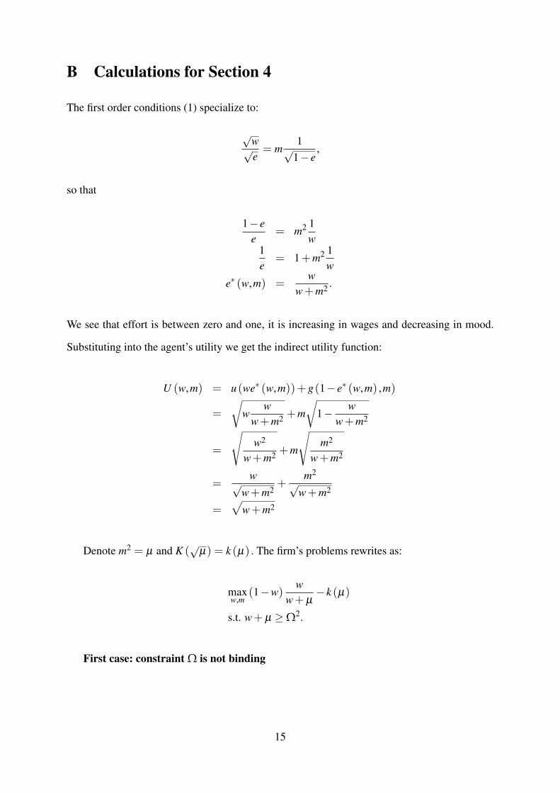
B Calculations for Section 4

The first order conditions (1) specialize to:

√w√e= m

1√1− e

,

so that

1− ee

= m2 1w

1e

= 1+m2 1w

e∗ (w,m) =w

w+m2 .

We see that effort is between zero and one, it is increasing in wages and decreasing in mood.

Substituting into the agent’s utility we get the indirect utility function:

U (w,m) = u (we∗ (w,m))+ g (1− e∗ (w,m) ,m)

=

√w

ww+m2 +m

√1− w

w+m2

=

√w2

w+m2 +m

√m2

w+m2

=w√

w+m2+

m2√

w+m2

=√

w+m2

Denote m2 = µ and K (√

µ) = k (µ) . The firm’s problems rewrites as:

maxw,m

(1−w)w

w+ µ− k (µ)

s.t. w+ µ ≥Ω2.

First case: constraint Ω is not binding

15

Suppose first the constraint is not binding. Then the problem is:

maxw,m

(1−w)w

w+ µ− k (µ) .

Derivatives with respect to the optimization variables:

w.r.t. µ : − (1−w)w1

(w+ µ)2 − k′ (µ)

w.r.t. w : − ww+ µ

+(1−w)

((w+ µ)−w

(w+ µ)2

)

= − ww+ µ

+(1−w)

(µ

(w+ µ)2

)

=−w (w+ µ)+ (1−w)µ

(w+ µ)2

=−w2−2wµ + µ

(w+ µ)2

=−w2−2wµ−µ2 + µ2 + µ

(w+ µ)2

=− (w+ µ)2 + µ2 + µ

(w+ µ)2

= −1+µ2 + µ

(w+ µ)2

In this case the derivative with respect to µ is always negative, so it is optimal to set µ as

small as possible, which we now assume is 1. The derivative with respect to w is decreasing in

w, so we have concavity, and for µ = 1 the derivative equals

−1+2

(w+ 1)2 .

Setting this equal to zero yields:

2

(w+ 1)2 = 1

2 = (w+ 1)2

w∗ =√

2−1 = 0.41421.

16

All of this makes sense. No sense in investing in mood since that only decreases effort and costs

money. Then you get an optimal wage.

To check whether the constraint is binding, substitute this value in the constraint:

Ω2 ≤ w∗+ µ∗ =√

2.

When Ω2 >√

2 the constraint is binding.

Second case: constraint Ω is binding

In this case the firm’s problem is:

maxw

(1−w)w

Ω2 − k(Ω2−w

)=

1Ω2 max

w(1−w)w−Ω2k

(Ω2−w

).

Since the term (1−w)w is increasing in w over (0.41421,0.5) and −Ω2k(Ω2−w

)is increas-

ing in w for all w’s, w∗ will never be below 1/2. This means that µ∗ = Ω2−w∗ is never above

Ω2−1/2.

The derivative with respect to w reads:

1−2w+Ω2k′(Ω2−w

).

If k (·) is a convex function this expression is decreasing in w so the first order conditions

identify an interior maximum w∗ (Ω) . Rewrite the first order conditions as follows:

(3) 1−2w = −Ω2k′(Ω2−w

).

Both sides of this equation are negative. Since −k′ (·) is a decreasing function, the right hand

side is an increasing function of w. As Ω2 increases to (Ω′)2 the right hand side becomes larger

in absolute value, and thus more negative, both because it gets scaled up by Ω2 and because k

is convex. Therefore w∗ (Ω′) > w∗ (Ω) .

17

Suppose K (m) = mα so that k (m) = mα/2 and k′ (m) = α

2 m(α/2)−1. Then (3) reads:

1−2w = −Ω2 (Ω2−w)α

2−1.

Now use the implicit function theorem:

∂

∂ Ω(1−2w∗ (Ω)) = − ∂

∂ ΩΩ2 (Ω2−w∗ (Ω)

)α

2−1

−2w∗′ (Ω) = −[2Ω(Ω2−w∗ (Ω)

)α

2−1+(2Ω−w∗′ (Ω))

(α

2−1)

Ω2 (Ω2−w∗ (Ω))α

2−2]

2w∗′ (Ω) = 2Ω(Ω2−w∗ (Ω)

)α

2−1+(2Ω−w∗′ (Ω))

(α

2−1)

Ω2 (Ω2−w∗ (Ω))α

2−2

2w∗′ (Ω) = Ω(Ω2−w∗ (Ω)

)α

2−1[2+(2Ω−w∗′ (Ω))

(α

2−1)

Ω(Ω2−w∗ (Ω)

)−1]

2w∗′ (Ω) = Ω (µ∗)α

2−1[

2+(2Ω−w∗′ (Ω))(

α

2−1) Ω

µ∗

]2

w∗′ (Ω)

Ω(µ∗)1−α

2 = 2+(2Ω−w∗′ (Ω))(

α

2−1) Ω

µ∗

2w∗′ (Ω)

Ω(µ∗)1−α

2 = 2+ 2(

α

2−1)Ω2

µ∗−w∗′ (Ω)

(α

2−1) Ω

µ∗

2w∗′ (Ω)

Ω(µ∗)1−α

2 +w∗′ (Ω)(

α

2−1) Ω

µ∗= 2+ 2

(α

2−1)Ω2

µ∗

w∗′ (Ω)

[2Ω

(µ∗)1−α

2 +(

α

2−1) Ω

µ∗

]= 2

(1+

(α

2−1)Ω2

µ∗

)

So finally

w∗′ (Ω) = 2(

1+(

α

2−1)Ω2

µ∗

).

1[2Ω (µ∗)1−α

2 +(

α

2 −1) Ω

µ∗

] .

18

Now, we are interested in:

∂ µ∗ (Ω)

∂ Ω=

∂

∂ Ω(Ω2−w∗ (Ω)

)= 2Ω−

2(

1+(

α

2 −1) Ω2

µ∗

)2Ω (µ∗)1−α

2 +(

α

2 −1) Ω

µ∗

= 2

Ω−

(1+

(α

2 −1) Ω2

µ∗

)2Ω (µ∗)1−α

2 +(

α

2 −1) Ω

µ∗

= 2

Ω[

2Ω (µ∗)1−α

2 +(

α

2 −1) Ω

µ∗

]−(

1+(

α

2 −1) Ω2

µ∗

)2Ω (µ∗)1−α

2 +(

α

2 −1) Ω

µ∗

= 22 (µ∗)1−α

2 +(

α

2 −1) Ω2

µ∗ −1−(

α

2 −1) Ω2

µ∗

2Ω (µ∗)1−α

2 +(

α

2 −1) Ω

µ∗

= 22 (µ∗)1−α

2 −12Ω (µ∗)1−α

2 +(

α

2 −1) Ω

µ∗

So ∂ µ∗(Ω)∂ Ω > 0 if and only if:

2 (µ∗)1−α

2 > 1

2 (µ∗)2−α

2 > 1

2(

1µ∗

)α−22

> 1(1

µ∗

)α−22

>12

1µ∗

>1

22

α−2

µ∗ < 2

2α−2

This inequality is never true for α = ∞ and is always true for all values of µ∗ if α = 2.

19