Effect of land albedo, CO , orography, and oceanic heat transport … · of intermediate complexity...

Clim. Past, 2, 31–42, 2006www.clim-past.net/2/31/2006/© Author(s) 2006. This work is licensedunder a Creative Commons License.

Climateof the Past

Effect of land albedo, CO2, orography, and oceanic heat transporton extreme climates

V. Romanova1, G. Lohmann2,3, and K. Grosfeld2,3

1Institute of Oceanography, University of Hamburg, 20146 Hamburg, Germany2Alfred Wegener Institute for Polar and Marine Research, 27515 Bremerhaven, Germany3Department of Physics, University of Bremen, Otto-Hahn-Allee, 330440 Bremen, Germany

Received: 11 October 2005 – Published in Clim. Past Discuss.: 7 December 2005Revised: 2 June 2006 – Accepted: 2 June 2006 – Published: 30 June 2006

Abstract. Using an atmospheric general circulation modelof intermediate complexity coupled to a sea ice – slab oceanmodel, we perform a number of sensitivity experiments un-der present-day orbital conditions and geographical distribu-tion to assess the possibility that land albedo, atmosphericCO2, orography and oceanic heat transport may cause an ice-covered Earth. Changing only one boundary or initial con-dition, the model produces solutions with at least some ice-free oceans in the low latitudes. Using some combinationof these forcing parameters, a full Earth’s glaciation is ob-tained. We find that the most significant factor leading to anice-covered Earth is the high land albedo in combination withinitial temperatures set equal to the freezing point. Oceanicheat transport and orography play only a minor role for theclimate state. Extremely low concentrations of CO2 also ap-pear to be insufficient to provoke a runaway ice-albedo feed-back, but the strong deviations in surface air temperatures inthe Northern Hemisphere point to the existence of a strongnonlinearity in the system. Finally, we argue that the ini-tial condition determines whether the system can go into acompletely ice covered state, indicating multiple equilibria,a feature known from simple energy balance models.

1 Introduction

Investigations of glacial carbonate deposits suggest a se-quence of extreme Neoproterozoic climate events (600–800million years ago). Paleolatitude indicators and paleomag-netic data (Hoffman, et al., 1998; Schmidt and Williams,1995; Sohl et al., 1999; Evans et al., 2000) imply widespreadequatorial glaciation at sea level. It was hypothesised thatthe Earth was completely ice covered (Kirschvink, 1992;Hoffman et al., 1998; Kirschvink et al., 2000; Hoffman

Correspondence to:V. Romanova([email protected])

and Schrag, 2002). Still, the question remains, whether theEarth was completely ice covered (“hard snowball” Earth)or some tropical ocean areas remained ice free (“slushball”Earth), and which mechanism drove the climate system intothe glaciated state and which allowed the escape from it(Caldeira and Kasting, 1992). Such extreme climates in theEarth’s history provide the motivation to investigate underwhat conditions the climate system is susceptible to extremechanges.

Fraedrich et al. (1999) and Kleidon et al. (2000) used ageneral circulation model to investigate the land albedo ef-fect of homogeneous vegetation extremes – global desert andglobal forest. It was found that the dominant signal is re-lated to changes in the hydrological cycle and that the al-tered water and heat balance at the surface has a potential im-pact on regional climate. Kubatzki and Claussen (1998) andWyputta and McAvaney (2001) showed that during the LastGlacial Maximum (LGM) the land albedo increased by 4%due to vegetation changes. In addition to this, the influence ofthe mountain chains and highly elevated glaciers with strongice albedo feedback leads to large climate anomalies andan alteration of the atmospheric circulation and precipitationpatterns (Lorenz et al., 1996; Lohmann and Lorenz, 2000;Romanova et al., 2005). The increase of the oceanic heattransport is also considered to be a crucial factor to preventEarth’s glaciation. For example, Poulsen et al. (2001) inves-tigated the role of the oceanic heat transport in ’snowball’Earth simulations and concluded that it could stop the south-ward advance of glaciers, such that a global glaciation on theEarth could not occur. Multiple stable equilibria are found inan aqua-planet simulation performed with a coupled atmo-spheric general circulation model with respect to change ofthe oceanic heat transport and initial conditions (Langen andAlexeev, 2004): one warm and ice free planet and one coldand icy climatic state. Furthermore, the atmospheric CO2level could also lead to a climate instability and a runawaysea-ice albedo mechanism (Poulsen, 2003). The magnitude

Published by Copernicus GmbH on behalf of the European Geosciences Union.

32 V. Romanova et al.: Extreme climates

of the atmospheric greenhouse gas concentrations, causingglaciation, is still under intense debate (e.g. Chandler andSohl, 2000; Donnadieu et al., 2004).

In this study, we are interested in the sensitivity of the cli-mate to changes of the land albedo, orography, oceanic heattransport and CO2 concentration. Using an AGCM of in-termediate complexity we investigate the climate responseto some extreme configurations of the boundary conditions.Therefore, we perform numerical experiments with differ-ent land albedo values and analyse scenarios, in which theland is completely covered with oak forests or glaciers. Wehave chosen sensitivity experiments with extreme orograph-ical and oceanic heat transport forcings, and with respect tothe snowball Earth hypothesis, we vary the CO2 concentra-tions to some extreme values. We left the land-sea geometryto present or to Last Glacial Maximum distributions. Mostof the external parameters which are different of extremeclimate states in the earth history (snowball Earth) are heldfixed in order to isolate the effect of land albedo, CO2, andoceanic heat transport with fixed parameters. Our approachis therefore intended as a sensitivity study.

The paper is organized as follows: in Sect. 2 the modelis briefly described and in the Sect. 3 the results are given.In Sect. 4 the results are discussed and final conclusions aregiven in Sect. 5.

2 Methodology

2.1 Model design

The atmospheric general circulation model (AGCM) used inour study is PUMA (Portable University Model of the Atmo-sphere) developed in Hamburg (Fraedrich, 1998; Lunkeit etal., 1998). It is based on the primitive equations transformedinto dimensionless equations of the vertical component of ab-solute vorticity, the horizontal divergence, the temperature,the logarithm of the surface pressure and the specific humid-ity. The equations are solved using the spectral transformmethod (Orszag, 1970; Eliasen et al., 1970), in which thevariables are represented by truncated series of spherical har-monics with wave number 21. The calculations are evaluatedon a longitude/latitude grid of 64 by 32 points, which corre-sponds approximately to a 5.6◦ resolution in Gaussian grid.In the vertical direction five equally spaced, terrain-followingsigma levels are used. The land and soil temperatures, soilhydrology and river runoff are parameterized in the model.

PUMA is classified as a model of intermediate complex-ity (Claussen et al., 2002) and it is designed to be compara-ble with comprehensive AGCMs like ECHAM (Roeckner etal., 1992). Previously, it was used to study stormtracks andbaroclinic life cycles (e.g. Frisius et al., 1998; Franzke et al.,2000) and to investigate multidecadal atmospheric responseto the North Atlantic sea surface temperatures (SST) forcing

(Grosfeld et al., 20061) as well as to simulate glacial climates(Romanova et al., 2005).

PUMA is coupled to a mixed layer ocean model, whichallows the prognosis of the sea surface temperatures (SST).The mixed layer ocean is forced with the oceanic heat trans-port and its depth is fixed at 50 m. A simple zero layer ther-modynamic sea ice model is also included. The temperaturegradient in the sea ice is linear and eliminates the capacityof the ice to store heat. Sea ice is formed if the ocean tem-perature drops below the freezing point (–1.9◦C), and meltswhenever the ocean temperature increases above this point.The albedo for sea iceRice, glaciersRgl and snow-coveredareasRsn is a linear function of the surface temperature,

Rsn,gl= R

sn,glmax + (R

sn,gl

min − Rsn,glmax )

Ts − 263.16

10(1)

Rice= min(Rice

max, 0.5 + 0.025(273.0 − Ti)) (2)

where,Ts andTi are the surface temperature over land andsea ice, respectively. The maximum albedo for sea ice isRice

max=0.7, the minimum and maximum albedo for glaciers

areRgl

min=0.6 andRglmax=0.8, and that for snow varies from

Rsnmin = 0.4 to Rsn

max = 0.8. The albedo of water is set to0.069.

2.2 Model set-up

To initialise the control run, a spin-up run (Expprescr, Ta-ble 1) is performed with prescribed SSTs and sea ice margins.The values of the global SST are taken to be equal to theclimatological mean for the time period between 1979 and1994 from the Atmospheric Model Intercomparison Project(AMIP) (Phillips et al., 1995). The CO2 concentration isfixed at 360 ppm. The orography and land-sea masks areset to present-day conditions. An equilibrium state of thespin-up run is obtained after 50 model years. The calcu-lated 10 years monthly averaged total surface heat fluxesfrom Exp prescr are taken to be equal to the oceanic heatfluxes, which serve as a forcing for the mixed layer oceanmodel. Thus, the oceanic heat transport is prescribed forthe coupled simulations and is taken to be the same for allsensitivity studies described below, except for those whichinvestigate the impact of zero oceanic heat transport. Themaximum value of the oceanic heat transport is 1.0 PW at30◦ N (Butzin et al., 2003; Romanova et al., 2005; Butzinet al., 2005) and represents a realistic value for present-dayconditions (Macdonald and Wunsch, 1996). The simulation,forced with the present-day heat transport and in which thealbedo is simulated by the model, is called the “control run”(Exp slab, Table 1). For all experiments, the Earth’s orbital

1Grosfeld, K., Lohmann, G., Rimbu, N., Lunkeit, F., andFraedrich, K.: Atmospheric multidecadal variations in the NorthAtlantic realm derived from proxy data, observations, and modelstudies, J. Geophys. Res., submitted, 2006.

Clim. Past, 2, 31–42, 2006 www.clim-past.net/2/31/2006/

V. Romanova et al.: Extreme climates 33

Sensitivity experiments CO2 Orography Abbreviation

AMIP (prescribed at the surface) 360 Present-day Exp_prescr

10 years averaged surface heat

fluxes from exp. Exp_prescr

360 Present-day Exp_slab

(control run)

Albedo albedo land - 0.2

albedo ocean - 0.069

Exp_alb02

albedo land - 0.8

albedo ocean - 0.069

Exp_alb08

albedo land: 0.8

initial temp: - 1.9° C

heat transport: zero

360

Present-day

Exp_IP

(ice-planet)

albedo land: 0.8


heat transport: PD

ExpIP_HfPD

albedo land: 0.8

initial temp: PD


ExpIP_iniTempPD

albedo land: free



ExpIP_albfree

Sensitivity

toward

initial and

boundary

conditions

Initial state Exp_IP

Albedo land: free

Heat transport: zero

360

Present-day

ExpIP_iniIP

CO2 – 1 ppm 1 Present-day Exp_1

CO2 - 10 ppm 10 Present-day Exp_10





Zero orography 360 Zero Exp_flat

Glacial orography 360 (Peltier 1994) Exp_glac

Zero heat transport 360 Present-day Exp_zero

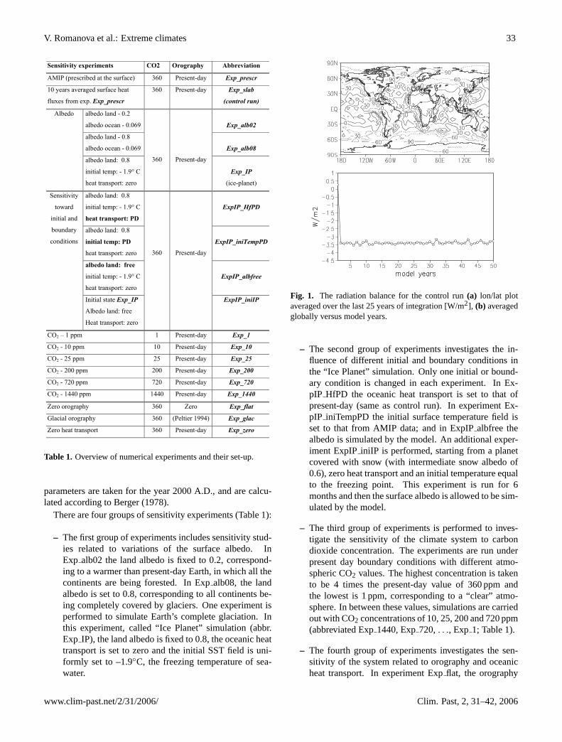
Table 1. Overview of numerical experiments and their set-up.

parameters are taken for the year 2000 A.D., and are calcu-lated according to Berger (1978).

There are four groups of sensitivity experiments (Table 1):

– The first group of experiments includes sensitivity stud-ies related to variations of the surface albedo. InExp alb02 the land albedo is fixed to 0.2, correspond-ing to a warmer than present-day Earth, in which all thecontinents are being forested. In Expalb08, the landalbedo is set to 0.8, corresponding to all continents be-ing completely covered by glaciers. One experiment isperformed to simulate Earth’s complete glaciation. Inthis experiment, called “Ice Planet” simulation (abbr.Exp IP), the land albedo is fixed to 0.8, the oceanic heattransport is set to zero and the initial SST field is uni-formly set to –1.9◦C, the freezing temperature of sea-water.

Fig. 1. The radiation balance for the control run(a) lon/lat plotaveraged over the last 25 years of integration [W/m2], (b) averagedglobally versus model years.

– The second group of experiments investigates the in-fluence of different initial and boundary conditions inthe “Ice Planet” simulation. Only one initial or bound-ary condition is changed in each experiment. In Ex-pIP HfPD the oceanic heat transport is set to that ofpresent-day (same as control run). In experiment Ex-pIP iniTempPD the initial surface temperature field isset to that from AMIP data; and in ExpIPalbfree thealbedo is simulated by the model. An additional exper-iment ExpIPiniIP is performed, starting from a planetcovered with snow (with intermediate snow albedo of0.6), zero heat transport and an initial temperature equalto the freezing point. This experiment is run for 6months and then the surface albedo is allowed to be sim-ulated by the model.

– The third group of experiments is performed to inves-tigate the sensitivity of the climate system to carbondioxide concentration. The experiments are run underpresent day boundary conditions with different atmo-spheric CO2 values. The highest concentration is takento be 4 times the present-day value of 360 ppm andthe lowest is 1 ppm, corresponding to a “clear” atmo-sphere. In between these values, simulations are carriedout with CO2 concentrations of 10, 25, 200 and 720 ppm(abbreviated Exp1440, Exp720,. . ., Exp 1; Table 1).

– The fourth group of experiments investigates the sen-sitivity of the system related to orography and oceanicheat transport. In experiment Expflat, the orography

www.clim-past.net/2/31/2006/ Clim. Past, 2, 31–42, 2006


Global Temperature (ºC)

Exp. name ANM DJF JJA

Planetary Albedo

(in fraction)

Surface Albedo

(in fraction)

control 17.00 15.84 18.36 0.31 0.17

Exp_alb02 18.33 17.21 19.65 0.31 0.12

Exp_alb08 -0.36 -1.26 1.10 0.41 0.39

Exp_IP -50.58 -49.20 -52.11 0.69 0.73

ExpIP_HfPD -50.84 -49.61 -52.23 0.69 0.73

ExpIP_iniTempPD -1.02 -2.76 1.21 0.42 0.38

ExpIP_albfree 16.14 14.66 17.15 0.32 0.18

ExpIP_iniIP 2.94 1.23 5.17 0.39 0.33

Exp_1 -6.75 -6.73 -6.76 0.40 0.39

Exp_10 0.15 -0.50 1.35 0.37 0.33

Exp_25 7.61 6.84 8.97 0.33 0.26

Exp_200 14.25 13.03 15.85 0.32 0.20

Exp_720 19.35 18.20 20.76 0.32 0.15

Exp_1440 21.64 20.54 22.99 0.32 0.13

Exp_glac 13.96 12.54 15.80 0.33 0.23

Exp_flat 18.23 17.02 19.70 0.31 0.16

Exp_zero 16.19 14.75 17.96 0.32 0.17

Table 2. Annual mean, DJF and JJA surface air temperatures (SAT)and globally averaged surface and planetary albedo.

is taken to be zero and in the experiment Expglac theorography and the glacial mask are the glacial ones asgiven by Peltier (1994) for the LGM. In the experimentExp zero, oceanic heat transport of zero W/m2 is ap-plied to the mixed layer model (Table 1).

The experiments are integrated over 50 years, when theyreach the equilibrium state. Figure 1 shows the balance be-tween the surface heat flux and the heat flux at the top of theatmosphere for the control run (the deviation from the zerobalance are due to water phase transitions and model errors,which are not included in the balance). No trend is foundafter the first year of the calculation, showing that the initialconditions are very close to the state of the model equilib-rium. Longer integrations, up to 25 years (Fig. 4) are nec-essary for the experiments driven with extreme initial andforcing conditions. All results shown represent annual meansaveraged over the last 25 years of integration.

3 Results and analyses

3.1.1 Sensitivity related to changes of the land albedo

The annual mean spatial pattern of the surface air tempera-tures (SAT) for the control run, for the experiments with pre-scribed surface albedo of 0.2 and 0.8, and for the ice-planetsimulation are shown in Fig. 2. The grey shading indicatesthe sea-ice coverage. A slight decrease of the land albedo to0.2 (Expalb02, Fig. 2b) compared to the present day sim-ulation (control run, Fig. 2a) leads to a global warming ofaround 1◦C (Table 2) and a retreat of the sea-ice margin.Especially in high latitudes, the SAT increases and the seaice retreats along the Antarctic coast. Contrary, a drastic in-crease of the albedo over the land to 0.8 (Fig. 2c), results

in a decrease of the global annual mean SAT by about 18◦C(Table 2) and the temperature at the equator of the AtlanticOcean is less than 15◦C (Fig. 2c). Sea-ice is formed closer tothe equator as its margin reaches 40◦ N and 50◦ S. The exper-iment ExpIP shows a full Earth glaciation. The global meantemperature falls to approximately –50◦C, and over Antarc-tica –80◦C are reached (Fig. 2d).

The calculated globally averaged surface albedo and theplanetary albedo (Table 2) show that the planetary albedo islarger by 82% and 158% than the surface albedo in the con-trol run and Expalb02, due to the high rates of evaporationand cloud formation. In experiment Expalb08 it is only 5%.In contrast to this, the surface albedo in the ice planet simula-tion (Exp IP) is larger (approximately 6%) than the planetaryalbedo.

3.1.2 Sensitivity of the Ice Planet simulations

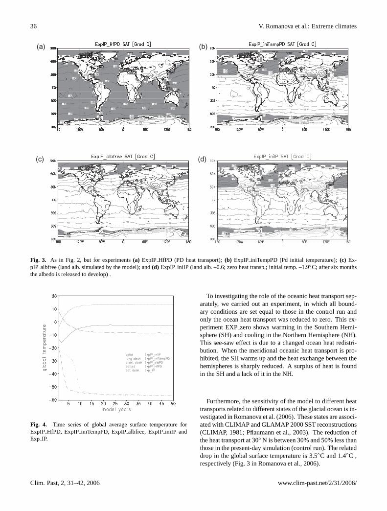
To isolate the effect and to determine the importance of eachboundary and initial conditions, sensitivity experiments ofthe Ice Planet simulation are performed, holding only oneof the boundary conditions the same as in the case of thecontrol run. Changing the heat transport to present-day val-ues, the model simulation does not generate any consider-able change in the SAT pattern (Fig. 3a). The temperaturesincrease by only 0.26◦C, but the earth remains ice coveredin the equilibrium state, which is reached about 5 years laterthan in the ExpIP (Fig. 4). If the initial temperature is set topresent day (AMIP) values, the planet does not end in a fullglaciation, although strong sea-ice formation in the North-ern Hemisphere occurs and the global temperature is almost20◦C lower compared to the control run (Table 2 and Fig. 4).Leaving the land albedo free to develop in ExpIPalbfree, theglobal temperature increases to about 16◦C (Fig. 3c) and thespatial temperature pattern tends to resemble the control run.An increase of the temperature (of about 10◦C) also occursin the experiment ExpIPiniIP, in which the land albedo wasreleased free to develop after 6 months of the Ice Planet in-tegration (Fig. 3d, Fig. 4). The relation between the surfaceand planetary albedo in the last two sensitivity experimentsis similar to the present-day conditions (the planetary albedois larger than the surface albedo), characterised by an evapo-ration regime and cloud formation (Table 2).

The decrease of temperature in the first two sensitivity ex-periments shows that the oceanic heat transport and the initialtemperature are not sufficient to prevent the global cooling.The global glaciation occurs independently of the oceanicheat transport. In contrast to this, the increased land albedoprovokes the planet’s warming and appears to be the mostimportant factor for the change of the climate system.



(a) (b)

(c) (d)

Fig. 1Fig. 2. Spatial pattern of the annual mean surface air temperatures averaged over a period of 25 years of integration for experiments(a)control run;(b) Exp alb02;(c) Exp alb08; and(d) Exp IP (land alb. set to 0.8; initial temp. set to –1.9◦C; the oceanic heat transport is zero).The grey shading indicates the annual mean sea-ice cover.

3.1.3 Sensitivity of the climate system to CO2 concentra-tion

A fourfold increase of CO2 concentration relative to present-day values, results in a more than 4◦C increase of the globaltemperature, and a two fold increase of the CO2 concentra-tion provokes a 2◦C global warming (Table 2). Reduction ofCO2 to 1 ppm results in a global cooling of 25◦C comparedto the control run, yielding an annual mean SAT of –7◦Cin EXP 1. In Fig. 5 the SAT and the sea-ice margin evolu-tion for experiments with CO2 concentration of 200, 25, 10and 1 ppm are shown. Reduction of CO2 cools the planet,sea-ice is formed closer to the equator, and the positive ice-albedo feedback is initiated. Nevertheless, the reduction ofCO2 under present-day geography and orbital conditions isnot sufficient to cause a full glaciation of the planet. Thedependence of the annual mean surface temperature on thelog (CO2) shows a good linear approximation (Fig. 6) con-sistent to, e.g., Budyko (1982), Manabe and Bryan (1985),and Oglesby and Saltzman (1990), and is valid not only forthe CO2 values near the present day concentration but alsofor the extreme concentrations as 1 ppm and 1440 ppm.

3.2 Orography and oceanic heat transport

In Fig. 7 the spatial SAT pattern of the experiments inves-tigating the role of orography and ocean heat transport areshown. Applying zero orography (EXPflat), the simulationshows global warming of 1◦C (Table 2). Over land, the im-pact is more obvious, as the temperature anomaly can reachup to 8◦C in the Himalaya Massive and around 22◦C in theAntarctic (Fig. 7a). Warming also occurs over the Pacific andalmost over the entire Atlantic. Still, cooling is noted in someareas of the North Atlantic and the whole Southern ocean (upto –2◦C).

The experiment forced with glacial orography (Peltier,1994) and present-day heat transport generates cooling(globally about 3◦C, Fig. 7b). Strong North American, NorthAtlantic, and Eurasian cooling of –16◦C to –20◦C is due tothe highly elevated Laurentide Ice Sheet, influencing gen-erally the atmospheric circulation pattern (Romanova et al.,2005). Along with a global cooling, an equatorial Pacificwarming is found, a feature similar to that in the CLIMAP(1981) reconstruction of the Last Glacial Maximum.



(a) (b)

(c) (d)

Fig. 2Fig. 3. As in Fig. 2, but for experiments(a) ExpIP HfPD (PD heat transport);(b) ExpIP iniTempPD (Pd initial temperature);(c) Ex-pIP albfree (land alb. simulated by the model); and(d) ExpIP iniIP (land alb. –0.6; zero heat transp.; initial temp. –1.9◦C; after six monthsthe albedo is released to develop) .

Fig. 3Fig. 4. Time series of global average surface temperature forExpIP HfPD, ExpIPiniTempPD, ExpIPalbfree, ExpIPiniIP andExp IP.

To investigating the role of the oceanic heat transport sep-arately, we carried out an experiment, in which all bound-ary conditions are set equal to those in the control run andonly the ocean heat transport was reduced to zero. This ex-periment EXPzero shows warming in the Southern Hemi-sphere (SH) and cooling in the Northern Hemisphere (NH).This see-saw effect is due to a changed ocean heat redistri-bution. When the meridional oceanic heat transport is pro-hibited, the SH warms up and the heat exchange between thehemispheres is sharply reduced. A surplus of heat is foundin the SH and a lack of it in the NH.

Furthermore, the sensitivity of the model to different heattransports related to different states of the glacial ocean is in-vestigated in Romanova et al. (2006). These states are associ-ated with CLIMAP and GLAMAP 2000 SST reconstructions(CLIMAP, 1981; Pflaumann et al., 2003). The reduction ofthe heat transport at 30◦ N is between 30% and 50% less thanthose in the present-day simulation (control run). The relateddrop in the global surface temperature is 3.5◦C and 1.4◦C ,respectively (Fig. 3 in Romanova et al., 2006).



(a) (b)

(c) (d)

Fig. 4Fig. 5. As in Fig. 2, but for experiments(a) Exp 200;(b) Exp 25; (c) Exp 10; and(d) Exp 1. The numbers denote the CO2 concentration.

3.3 Zonal mean SAT anomalies

An overview of the zonally averaged temperature anomaliesrelative to the control run is shown for all experiments inFig. 8. The first panel represent the temperature anomaliesfor EXP glac, EXPflat and EXPzero. Strong midlatitudeand polar region cooling in the NH and SH, due to the ex-tended glacial ice sheets, is found in EXPglac. The see-saw effect between the NH and SH characterises the resultsof EXP zero and an overall warming except in the SouthernOcean is found in EXPflat. On the second panel (Fig. 8b)the SAT anomalies for the experiments with changed albedoare displayed. EXPalb02 shows a small increase of the tem-perature (around 1◦C) relative to the present-day simulation,except for the Antarctic, where the sharp change of surfacereflectivity from glaciers (0.8) to forest (0.2) yields a warm-ing of nearly 10◦C; EXP alb08 exhibits strong, zonal coolingup to –30◦C in mid and high northern latitudes, indicatingthe opposite effect than in EXPalb02 for the Antarctic; andin EXP IP the temperature anomaly can reach –70◦C in theequatorial and tropical latitudes. The third panel visualizesthe temperature reduction in the NH due to the reduction ofCO2 and the consequential positive ice-albedo feedback. Theextreme experiment EXP1 exhibits very strong anomalies,up to –40◦C SAT in the subtropics in the NH.

1 10 100 1000

-10

-5

0

5

10

15

20

25

1 ppm

10 ppm

1440 ppm

720 ppm

200 ppm25 ppm

360 ppm

AN

MS

urface

Tem

pera

ture

[Cº ]

CO2

[ppm]

Fig. 5

Fig. 6. Log plot of the carbon dioxide concentration versus ANMsurface temperature for exp. Exp1, Exp 10, Exp25, Exp200,Exp 360, Exp720 and Exp1440. The line shows the linear fit.

3.4 Zonal mean precipitation

To assess the Hadley circulation and the Intertropical Conver-gence Zone (ITCZ) for different sensitivity experiments theaveraged zonal mean precipitation is calculated. The zonal



(a)

(c)

(b)

Fig. 6

Fig. 7. Annual mean surface air temperatures anomalies:(a)Exp flat-control run (zero orography);(b) Exp glac-control run(LGM orography given by Peltier, 1981); and(c) Exp zero-controlrun (zero heat transport). The grey shading indicates the positiveanomalies.

mean boreal winter and summer values for the sensitivity ex-periments are shown in Fig. 9. The maximum precipitationin boreal winter for the present-day simulation is situated inthe SH, while in the boreal summer it is located in the NH.

The experiments investigating the effect of the orography(Fig. 9a, b) EXPflat and EXPglac show seasonal deviationsfrom the present-day values. In EXPflat the maximum pre-

(a)

(c)

(b)

Fig. 7

Tem

pera

ture

anom

aly

Tem

pera

ture

anom

aly

Tem

pera

ture

anom

aly

Fig. 8. Zonal mean of the global surface temperature anomaliesrelative to the control run:(a) effect of orography and oceanic heattransport;(b) changed land albedo and Ice Planet simulation; and(c) different CO2 concentrations in the atmosphere.

cipitation during boreal winter is reduced, while in EXPglacit is enhanced. The opposite tendency is found in boreal sum-mer, EXPflat shows an increase in precipitation and exper-iment EXPglac produces a decrease. The land elevation inthe NH results in pronounced seasonality in the equatorialregion. As the orography is higher, the ITCZ is strengthenedin boreal winter and is suppressed in boreal summer. The ab-sence of heat transport in EXPzero increases the maximumprecipitation in both seasons, compared to the control run.

The precipitation in the land albedo experimentEXP alb02 is similar to the present-day’s one, exceptin the region of Antarctica, where the drastic change ofthe albedo produces a peak in precipitation in winter(Fig. 9cd). In EXPalb08 the precipitation maximum isstrongly shifted to the SH (around 15◦ S) and located in thebelt of all-years SAT maximum. The magnitude is 20%less than the present-day value. A decrease in precipitation



(a)

(e)

(c)

Fig. 8

(b)

(f)

(d)

Fig. 9. The DJF and JJA zonal mean precipitation for control run (solid line) and(a, b) the experiments investigating the effect of orographyand oceanic heat transport;(c, d) experiments with changed land albedo and Ice Planet simulation; and(e, f) experiments with different CO2concentrations.

occurs in the midlatitudes of the NH and SH due to theextensive ice-coverage and negative surface temperatures.The ice-covered planet in EXPIP prohibits precipitation thewhole year round.

The experiment with a fourfold present-day CO2 concen-tration shows a decrease in the precipitation during borealwinter and an increase during boreal summer (Fig. 9ef).The tendency is the same as in EXPflat (described earlier),whereas the experiment with CO2 equal to 200 ppm exhibitsthe tendency of EXPglac – an increase in the precipitationduring boreal winter and decrease during boreal summer.Therefore, glacial orography and the reduction of CO2 actin the same direction. Both change the ITCZ and Hadley cir-culation in equatorial and tropical latitudes. In experimentEXP 1 the precipitation is considerably lowered, as its max-imum does not experience seasonality and is always locatedin the SH, tending to the same result as in EXPalb08.

4 Discussions

We investigate the sensitivity of the climate to some extremeboundary and initial conditions and combinations of extremeparameters under present-day insolation and continental dis-tributions. Examining the influence of each factor, we assessthe role of the land albedo, the influence of high and low CO2concentration levels, the importance of the orography and ofthe oceanic heat transport.

The experiments with only one parameter changed, showequilibrium states, in which the equatorial ocean remains ice-free. Using a combination of extreme boundary and initialconditions, like zero oceanic heat transport, high land albedoand the initial temperature uniformly set to a value equal tothe freezing point, an ice-covered Earth under present-dayorbital parameters and CO2 concentration can be attained.Further investigation of the experiments with a combinationof two of the mentioned extreme boundary conditions, showsthat the dominant factor for the decrease of temperature in the



ice planet simulation is the land albedo. If the land albedois a variable parameter, independently of the zero oceanicheat transport or the low initial temperature field, the tem-peratures increase and tend to reach the values of the con-trol run. Interestingly, the present-day oceanic heat transportalone is not able to produce ice-free equatorial oceans. Afull glaciation is delayed but successfully reaches the ice-planet equilibrium (Fig. 4). Even though the heat transportof the present-day climate seems not to be appropriate withrespect to ice-covered oceans (Poulsen et al., 2001; Lewiset al., 2003), its role appears to be negligible compared tocontinental surface properties. Using a 2,5 dimensional cou-pled climate model of intermediate complexity, Dounadieu etal. (2004) concluded that the dynamic oceanic process can-not prevent the onset of the ice-albedo instability in a Neo-proterozoic simulation. Another factor prohibiting the for-mation of an ice-covered planet is the high initial tempera-ture field (set to present-day values). Although the globaltemperature falls approximately 20◦C, the sea-ice cover ad-vance is restricted up to 30◦ N and 60◦ S. The asymmetricaldistribution of the sea-ice margins is more sensitive to the pa-leogeography differences than to the change of other param-eters, e.g., the insolation (Poulsen et al., 2002). Releasing theland albedo after the 20-th year of the ice planet simulation(not shown) does not infer any change in the climate system,due to the very low temperatures, which force the land andice albedo to attain their maximal values. Thus, the ice planetsimulation reaches a stable climate and only an external in-fluence can lead to change of this stable state (e.g., increaseof carbon dioxide due to strong volcanic activity and lack ofchemical weathering).

Does the orography matter in the initiation of extreme cli-mate? The LGM reconstruction of the orography (Peltier,1994), including the highly elevated Laurentide Ice Sheet,reduces the global temperature by 3◦C. The influence ofchanged orography predominates in the contribution to theNorthern Hemispheric cooling, but it is of no importanceto the tropics. Thus the altered orography is more impor-tant in regional sense, than in global. Jenkins and Frakes(1998) introduced a 2 km north-south mountain chain on thesuper continent in their Neoproterozoic model set up, andshowed that the orogeny could not be considered as a factorfor the global glaciation. But it can redistribute the humidityover sea-ice and thus, change the hydrological cycle (Don-nadieu et al., 2003). However, the climate system responsesnonlinearly to linear change of the height of the ice-sheet(Romanova et al., 2005), which points to the existence of athreshold, over which a runaway albedo feedback over theAmerican continent could be initiated. Further investigationof the sensitivity of the climate system toward enlargement ofthe Laurentide Ice Sheet could be of interest when searchingfor this threshold.

The experiments control run, EXPalb02, EXPflat,EXP 1440 showed a planetary albedo larger than the sur-face albedo (in some cases more than 150%), due to the

strong evaporation over the ice-free oceans and cloud for-mation. In the experiments (EXPalb08, EXPIPiniTempPDand EXP1), in which the absolute global temperature isaround 0◦C and which are characterised by cold climaticconditions and ice-free equatorial and tropical latitudes, theglobal surface and planetary albedo tend to be in the sameorder. However, these cold climates (EXPalb08 and EXP1)could exhibit an intense equatorial precipitation maxima anda strong Hadley circulation due to the sharp temperaturegradients from the equator to the edge of the sea-ice mar-gin, which works against the positive ice-albedo feedback(Bendtsen, 2002). The hydrological cycle and the ITCZ arerather sensitive to the change of the surface temperature inthe tropics and to the strength of the Atlantic overturning(Lohmann and Lorenz, 2000; Lohmann, 2003). Interestingly,in the ice-planet experiments EXPIP and EXPIPiniIP, theestimates of the global planetary albedo appear smaller thanthe global surface albedo. On a completely glaciated Earth,the processes of evaporation, cloud formation and precipita-tion are strongly suppressed or even do not exist, thus theratio between the incident and reflected short wave radiationon the surface is higher than the ratio between the incidentand reflected/scattered short wave radiation on the top of theatmosphere. The loss of energy in the atmosphere could bedue to the process of water vapour absorption, where the wa-ter vapour is provided only by the process of sublimation.

5 Concluding remarks

Motivated by the early work with EBMs (Budyko, 1969;Sellers, 1969) and the discussion about an ice covered Earth(e.g., Crowley and Baum, 1993; Jenkins and Frakes, 1998;Hyde et al., 2000; Chandler and Sohl, 2000; Crowley et al.,2001; Poulsen et al., 2001; Donnadieu et al., 2002, 2004;Bendtsen, 2002; Lewis et al., 2003; Stone and Yao, 2004), weinvestigate the possibility for extreme climates under presentconfigurations (continent distribution and orbital forcing) ina simplified AGCM coupled to a mixed layer-sea ice model(Fraedrich, 1998; Franzke et al., 2000; Grosfeld et al., 20061;Romanova et al., 2005).

Investigating the Neoproterozoic glaciations, many au-thors search for a CO2 threshold value. Different simula-tions show a sensitivity of the minimum CO2 level to con-tinental configurations (Poulsen et al., 2002; Donnadieu etal., 2004), Earth’s rotation rate and obliquity (Jenkins andSmith, 1999; Jenkins, 2000), solar luminosity (Crowley etal., 2001) oceanic heat transport (Poulsen et al., 2001) or anincrease of the albedo (Lewis et al., 2003). Our experimentsfor present day setup suggest that the reduction of atmo-spheric CO2 alone is not sufficient to provoke global glacia-tion under present-day insolation. We find a strong nonlin-earity in the NH at a CO2 concentration of 25 ppm. The tem-perature anomaly, relative to the present-day simulation, canreach –40◦C at 1 ppm. Our simulations show that the ini-



tial condition of the system is important when simulating asnowball Earth. Indeed, a hysteresis of the climate system isfound with respect to a change of the infrared forcing (Crow-ley et al., 2001) and solar constant (Stone and Yao, 2004).We suppose similar climate behaviour to a slow change ofthe CO2 concentration and a snow cover and we will addressthis question in our further research.

In our sensitivity experiments we evaluated extreme ef-fects of land albedo and CO2 on climate in a similar wayas Fraedrich et al. (1999) for vegetation extremes on theatmosphere. In our approach, we calculated the sea sur-face temperature interactively by assuming different oceanheat transports. We have neglected several climatic links be-tween the components, including e.g., the hydrological cy-cle/temperature, vegetation, weathering rates, carbon cycle,and deep ocean circulation. As a logical next step, more in-teractive climate components will be included in order to es-timate the most extreme climate states under present and pastclimate configurations. The combined effects yield differentregimes which are relevant to understand past climate evolu-tions as recorded, e.g., in cabonate deposites.

Acknowledgements.We gratefully acknowledge the suggestionsand recommendations of F. Lunkeit and thank K. Fraedrich forproviding us with the model code. We thank also M. Dima andK. Vosbeck for the improvement of the manuscript. This work hasbeen funded by the German Ministry for Education and Research(BMBF) within DEKLIM project “Climate Transitions” andMARCOPOLI.

Edited by: V. Masson-Delmotte

References

Bendtsen, J.: Climate sensitivity to changes in solar insolation in asimple coupled model, Clim. Dyn., 18, 595–609, 2002.

Berger, A. L.: Long term variations of daily insolation and quater-nary climatic changes, J. Atmos. Sci., 35(12), 2362–2367, 1978.

Budyko, M. I.: The effect of solar radiation variations on the climateof the Earth, Tellus, 21, 611–619, 1969.

Budyko, M. I.: The Earth’s climate: past and future, AcademicPress, New York, p. 307, 1982.

Butzin, M., Prange, M., and Lohmann, G.: Studien zur 14C-Verteilung im glazialen Ozean mit einem globalen Ozeanzirku-lationsmodell, Terra Nostra, 6, 86–88, 2003.

Butzin, M., Prange, M., and Lohmann G.: Radiocarbon simulationsfor the glacial ocean: the effects of wind stress, Southern Oceansea ice and Heinrich events, Earth Planet. Sci. Lett., 235, 45–61,doi:10.1016/j.epsl.2005.03.003, 2005.

Caldeira, K. and Kasting, J. F.: The life span of the biosphere revis-ited, Nature, 360, 721–723, 1992.

Chandler, M. A. and Sohl, L. E.: Climate forcings and the initiationof low-latitude ice sheets during Neoproterozoic Varanger glacialinterval, J. Geophys. Res., 105, 20 737–20 756, 2000.

Claussen, M., Mysak, L. A., Weaver, A. J., Crucifix, M., Fichefet,T., Loutre, M. F., Weber, S. L., Alcamo, J., Alexeev, V. A.,Berger, A., Calov, R., Ganopolski, A., Goosse, H., Lohmann, G.,

Lunkeit, F., Mokhov, I. I., Petoukhov, V., Stone, P., and Wang,Z.: Earth system models of intermediate complexity: Closingthe gap in the spectrum of climate system models, Clim. Dyn.,18, 579–586, 2002.

CLIMAP Project Members: Seasonal reconstructions of the earth’ssurface at the Last Glacial Maximum, Geological Society ofAmerica, Map and Chart Series, MC-36, 18, 18 maps, 1981.

Crowley, T. J. and Baum, S. K.: Effects of decreased solar luminos-ity on Late Precambrian ice extent, J. Geophys. Res., 98, 16 723–16 732, 1993.

Crowley, T. J., Hyde, W. T., and Peltier, W. R.: CO2 levels requiredfor deglaciation of a ‘Near Snowball’ Earth, Geophys. Res. Lett.,28, 283–286, 2001.

Donnadieu, Y., Ramstein, G., Fluteau, F., Besse, J., and Meert, J.: Ishigh obliquity a plausible cause for Neproterozoic glaciations?,Geophys. Res. Lett., 29, doi:10.1029/2002GL015902, 2002.

Donnadieu, Y., Fluteau, F., Ramstein, G., Ritz, C., and Besse, J.: Isthere a conflict between the Neoproterozoic glacial deposits andsnowball Earth interpretation: an improved understanding withnumerical modeling, Earth Plan. Sci. Lett., 208, 101–112, 2003.

Donnadieu, Y., Ramstein, G., Fluteau, F., Roche, D., and Ganopol-ski, A.: The impact of atmospheric and oceanic heat trans-ports on the sea-ice-albedo instability during the Neoproterozoic,Clim. Dyn., 22, 293–306, 2004.

Eliasen, E., Machenhauer, B., and Rasmussen, E.: On a numericalmethod for integration of the hydrodynamical equations with aspectral representation of the horizontal fields, Report No. 2, In-stitute for Theoretical Meteorology, University of Copenhagen,37 pp., 1970.

Evans, D. A. D., Li, Z. X., Kirschvink, J. L., and Wingate, M.T. D.: A high-quality mid-Neoproterozoic paleomagnetic polefrom South China, with implications for ice ages and the breakupconfiguration of Rodinia, Precambrian Res., 100(1–3), 313–334,2000.

Fraedrich, K., Kirk, E., and Lunkeit, F.: Portable University Modelof the Atmosphere, Deutsches Klimarechenzentrum, Tech. Rep.,16, 377 pp., 1998.

Fraedrich, K., Kleidon, A., and Lunkeit, F.: A green planet versus adesert world: Estimating the effect of vegetation extremes on theatmosphere, J. Climate, 12, 3156–3163, 1999.

Franzke, C., Fraedrich, K., and Lunkeit, F.: Low frequency variabil-ity in a simplified atmospheric global circulation model: Stormtrack induced ‘spatial resonance’, Quat. J. Roy. Met. Soc., 126,2691–2708, 2000.

Frisius, T., Lunkeit, F., Fraedrich, K., and James, I. N.: Storm-trackorganization and variability in a simplified atmospheric globalcirculation model (SGCM), Quat. J. Roy. Met. Soc., 124, 1019–1043, 1998.

Hoffman, P. F. and Schrag, D. P.: The snowball Earth hypothesis:testing the limits of global change, Terra Nova, 14, 129–155,2002.

Hoffman, P. F., Kaufman, A. J., Halverson, G. P., and Scharg, D.P.: A Neoproterozoic snowball earth, Science, 281, 1342–1346,1998.

Hyde, W. T., Crowley, T. J., Baum, S. K., and Peltier, W. R.:Neoproterozoic “snowball Earth” simulations with a coupledclimate/ice-sheet model, Nature, 405, 425–429, 2000.

Jenkins, G. S.: Global climate model high-obliquity solutions tothe ancient climate puzzles of the Faint Young Sun Paradox and



low altitude Proterozoic Glaciation, J. Geophys. Res., 105, 7357–7370, 2000.

Jenkins, G. S. and Frakes, L. A.: GCM sensitivity test using in-creased rotation rate, reduced solar forcing and orography to ex-amine low latitude glaciation in the Neoproterozoic, Geophys.Res. Lett., 25, 3525–3528, 1998.

Jenkins, G. S. and Smith, S. R.: GCM simulation of Snowball Earthconditions during the late Proterozoic, Geophys. Res. Lett., 26,2263–2266, 1999.

Kirschvink, J. L.: Late proterozoic low-lattitude global glaciation:the Snowball Earth, in: The Proterozoic biosphere, edited by:Schopf, J. W. and Klein, C., Cambridge UK, pp 51–52, 1992.

Kirschvink, J. L., Gaidos, E. J., Bertani, E., Beukes, N. J., Gutzmer,J., Maepa, L. N., and Steinberger, R. E.: Paleoproterozoic snow-ball Earth: Extreme climatic and geochemical global change andits biological consequences, PNAS 97, 1400-14005, 2000.

Kleidon, A., Fraedrich, K., and Heimann, M.: A green planet versusa desert world: Estimating the maximum effect of vegetation onthe surface energy balance, Climatic Change, 44, 471–493, 2000.

Kubatzki, C. and Claussen, M.: Simulation of the global bio-geophysical interactions during the Last Glacial Maximum, Cli-mate Dynamics, 14, 461–471, 1998.

Langen, P. L. and Alexeev, V. A.: Multiple equilibria and asymmet-ric climates in the CCM3 coupled to an oceanic mixed layer withthermodynamic sea ice, Geophys. Res. Lett., L04201, 2004.

Lewis, J. P., Weaver, A. J., Johnston, S. T., and Eby, M.: Neo-proterozoic “snowball Earth”: Dynamic sea ice over a quies-cent ocean, Paleoceanography, 18, doi:10.1029/2003PA000926,2003.

Lohmann, G.: Atmospheric and oceanic freshwater transport duringweak Atlantic overturning circulation, Tellus, 55 A, 438–449,2003.

Lohmann, G. and Lorenz, S.: On the hydrological cycle under pale-oclimatic conditions as derived from AGCM simulations, J. Geo-phys. Res., 105, 417–436, 2000.

Lorenz, S., Grieger, B., Helbig, Ph., and Herterich, K.: Investigat-ing the sensitivity of the atmospheric general circulation modelECHAM 3 to paleoclimatic boundary conditions, Geol. Rund-sch., 85, 513–524, 1996.

Lunkeit, F., Bauer, S. E., and Fraedrich, K.: Storm tracks in awarmer climate: Sensitivity studies with a simplified global cir-culation model, Clim. Dyn., 14, 813–826, 1998.

Macdonald, A. M. and Wunsch, C.: An estimate of global oceancirculation and heat fluxes, Nature, 382, 436–439, 1996.

Manabe, S. and Bryan, K.: CO2-induced change in a coupledocean-atmosphere model and its paleo-climatic implications, J.Geophys. Res., 90, 11 689–11 707, 1985.

Oglesby, R. and Saltzman, B.: Sensitivity of the equilibrium surfacetemperature of a GCM to systematic changes in atmospheric car-bon dioxide, Geophys. Res. Lett., 17, 1089–1092, 1990.

Orszag, S. A.: Transform method for calculation of vector-coupledsums: Application to the spectral form of the vorticity equation,J. Atmos. Sci., 27, 890–895, 1970.

Peltier, W. R.: Ice age paleotopography, Science, 265, 195–201,1994.

Pflaumann, U., Sarnthein, M., Chapman, M., d’Abreu, L., Fun-nell, B., Huels, M., Kiefer, T., Maslin, M., Schulz, H., Swal-low, J., van Kreveld, S., Vautravers, M., Vogelsang, E., Weinelt,M.: Glacial North Atlantic: Sea-surface conditions recon-structed by GLAMAP 2000, Paleoceanography, 18(3), 1065,doi:10.1029/2002PA000774, 2003.

Phillips, T. J., Anderson, R., and Brosius, M.: Hypertext sum-mary documentation of the AMIP models, UCRL-MI-116384,Lawrence Livermore National Laboratory, Livermore, CA, 1995.

Poulsen, C. J., Pirrehumbert, R. T., and Jacob, R. L.: Impact ofocean dynamics on the simulation of the Neoproterozoic “snow-ball Earth”, Geophys. Res. Lett., 28, 1575–1578, 2001.

Poulsen, C. J., Jacob, R. L., Pierrehumbert, R. T., and Huynh, T.T.: Testing paleogeographic controls on a Neoproterozoic snow-ball Earth, Geophys. Res. Lett., 29, doi:10.1029/2001GL014352,2002.

Poulsen, C. J.: Absence of runaway ice-albedo feedback in the Neo-proterozoic, Geology, 31, 473–476, 2003.

Roeckner, E., Arpe, K., Bengtsson, L., Brinkop, S., Dumenil, L.,Esch, M., Kirk, E., Lunkeit, F., Ponater, M., Rockel, B., Sausen,R., Schlese, U., Schubert, S., and Windelband, M.: Simulation ofpresent-day climate with the ECHAM model: Impact of modelphysics and resolution. MPI Report No. 93, ISSN 0937-1060,Max-Planck-Institut fur Meteorologie, Hamburg, Germany, 171pp., 1992.

Romanova, V., Lohmann, G., Grosfeld, K., and Butzin, M.: Therelative role of oceanic heat transport and orography on glacialclimate, Quat. Sci. Rev., doi:10.1016/j.quascirev.2005.07.007,2005.

Schmidt, P. W. and Williams, G. E.: The Neoproterozoic climaticparadox; equatorial palaeolatitude for Marinoan Glaciation nearsea level in South Australia, Earth Planet. Sci. Lett., 134(1–2),107–124, 1995.

Sellers, W. D.: A global climatic model based on the energy balanceof the earth atmosphere system, J. Appl. Meteorol., 8, 392–400,1969.

Sohl, L. E., Christie-Blick, N., and Kent, D. V.: Paleomagnetic po-larity reversals in Marinoan (ca. 600 Ma) glacial deposits of Aus-tralia: implications for the duration of low-latitude glaciation inNeoproterozoic time, Geol. Soc. Am. Bull., 111(8), 1120–1139,1999.

Stone, P. H. and Yao, M. S.: The ice-covered Earth instability ina model of intermediate complexity, Clim. Dyn., 22, 815–822,doi:10.1007/s00382-004-0408-y, 2004.

Wyputta, U. and McAvaney, B. J.: Influence of vegetation changesduring the Last Glacial Maximum using the BMRC atmosphericgeneral circulation model, Clim. Dyn., 17, 923–932, 2001.


Effect of land albedo, CO , orography, and oceanic heat transport … · of intermediate complexity...

Documents

Transcript of Effect of land albedo, CO , orography, and oceanic heat transport … · of intermediate complexity...