i | P a g e

EFFECT OF CREDIT CONSTRAINTS ON INTENSITY OF FERTILZER ADOPTION AND AGRICLUTURAL

PRODUCTIVITY IN AMHARA REGION, ETHIOPIA: AN ENDOGENOUS SWITCHING REGRESSION ANALYSIS

Mulat Goshu Gebeyehu (MSc)

Lecture

Department of Economics

Wolaita Sodo University

Email: mulatgoshu@gmail.com

Cell phone: +251(0) 921936504

Acknowledgements

I am indebted to Dr. Assefa Admassie for his cooperation has allowed me to use EPIICA data set

and in the pursuit of institutions involved in the Ethiopian Project in Interlinking Insurance with

Credit in Agriculture to allowing me the data. I am grateful for institutions involved in the

Ethiopian Project in Interlinking Insurance with Credit in Agriculture for allowed me to use their

reach data set. These are university of California at San-Diego, university of Athens, university of

Greece and FAO, EEA, Dashen Bank and Nyala Insurance Company.

At the end, I would like to express my gratitude to my friends Mr. Tadele Tafesse, Mr. Ermias

Ganamo and Mr. Ayana Anteneh who have constantly provided invaluable guidance,

encouragement, and support throughout my study. Thank you!

ii | P a g e

Abstract

Access to finance to the rural households is a powerful intervention to facilitate the adoption of farm

inputs and boost agricultural productivity in developing countries like Ethiopia. Credit constraints limit

the ability of households to use inputs at optimal level and thereby stifles agricultural productivity.

However evaluation of the impact of credit constraints on agricultural technology adoption and

productivity have faced methodological problems and most of the existing studies have failed to

explicitly measure and analyze the amount of productivity loss and the magnitude increase in intensity of

fertilizer adoption if the farm households are found credit unconstrained. This study examines the

poetional impact of credit constraint on the intensity of fertilizer adoption and productivity among

households who vary in their credit constraint status. The study used cross sectional farm household level

data collected in 2013 from 1165 a randomly sampled households. An endogenous switching regression

model is used for analytical purpose so as to account for selection bias and heterogeneity problem. The

result evidence that intensity of fertilizer adoption and agriculture productivity would be higher among

farm households who are found to be credit unconstrained. The result revealed that factors that affect the

intensity of fertilizer adoption and agriculture productivity among credit constrained farm households are

different from their counterparts. Age and age square of the household head, primary cooperative

membership, number of Oxen, ownership of TV, hired labor as dummy and use of manure have significant

effect on the intensity of fertilizer adoption among credit unconstrained regimes. Whereas, household

size, altitude of land, ownership of land, way of land cultivation, and being risk averse household have

significant effect on the intensity of fertilizer adoption in the credit constrained regimes. The result shown

that size of land has negative and significant impact on the intensity of fertilizer adoption in the

constrained regime while it has positive and significant impact on the intensity of adoption in the

unconstrained regime. Age and age square of the household head, TLU, hired labor as dummy are the

factors that significantly affect the productivity in the unconstrained regimes. The number of oxen and

distance of farm land from residence also affect the productivity. Land size has found the significant and

negative effect on the productivity in the constrained regime, but it has the positive and significant effect

in the credit constrained regime. The policy implication is that the policy makers should account the

credit constraint heterogeneity among farm households when they design agricultural policy to increase

intensity of fertilizer adoption and thereby boost productivity of agriculture.

Key words: Credit constraint, agricultural productivity, intensity of fertilizer application, an

endogenous switching regression, Ethiopia

1 | P a g e

1. INTRODUCTION

Ethiopia has made significant economic and social progress towards reducing poverty over the

last decade. However, the country still remains one of the poorest countries in the world.

Ethiopia has a population over 93 million and agriculture is the main source of economic growth.

Agriculture contributes 40 percent to GDP and provides employment to about 72.7 percent of the

country‟s labor force. Additionally, agriculture contributes 90% of foreign exchange earning to

the country and the sector supplies raw material to manufacturing and service sectors (UNDP,

2015).

In Ethiopia, however, agriculture production is heavily dependent on rainfall. It is subject to a

variety of risks arising from erratic rainfall, drought, temperature fluctuations, hailstorms,

cyclones, floods, and climate change. Natural disasters, especially floods and droughts frequently

damaged the agricultural production in the country. These risks are exacerbated by price

fluctuations, a weak rural infrastructure, imperfect markets and lack of financial services

including limitations in the design of risk mitigation instruments such as credit and insurance

(MoA,2010). This evidence that rural population in Ethiopia has been unable to leave out of

poverty principally because they have not been able to transform their basic economic activity

which is agriculture.

To address the issue of poverty as clearly stated in Ethiopia‟s growth and transformation plan

(GTP), it is necessary that the constraints to agriculture should be solved. One main constraint

identified by different scholars and policy makers and so far not partly addressed is the lack of

access to finance. Ethiopia has a very low rural banking density and consequently one of the

lowest financial inclusion ratios in Sub-Saharan Africa, with only 14% of adults having access to

credit. Bank branches are concentrated in urban areas, while rural areas remain underserved.

Only 1% of the rural population has bank accounts (AGRIFIN, 2012). This evidences that the

significant portion of the rural people in Ethiopia do not have access to formal financial services.

Inadequate credit supply is a central problem along with which other production factors exert

negative influence on farmers‟ output and efficiency. These are due to the reason that poor are

unable to secure the required collateral and hence considered as not creditworthy by financial

institutions, such as banks. Lending to rural farm households is perceived as a risk endeavor

partly because of high loan default by farmers observed in many developing countries and the

fact that it involves high transaction costs (Assefa, 2004; Ali and Feininger 2012).

2 | P a g e

Generally, smallholders in Ethiopia are characterized by low or negligible saving, low capital

formation and very low or no non-farm income and are usually unable to adopt improved

technologies and increase productivity. Hence, the provision of timely credit with affordable

price has power full intervention to mobilizing resources from less productive use to more

productive uses and to alleviate poverty and food insecurity.

When liquidity is a binding constraint, the amount and combinations of inputs used by

smallholder farmers may deviate from optimal levels that in turn limit the optimum production or

consumption choices. The marginal contribution of credit, therefore, brings input levels closer to

the optimal levels and thereby increasing output (Feder et al., 1990; Imoudu and Onaksapnome,

1992; Diagne and Zeller, 2001). Credit constraint is one main source of low adoption and use of

modern inputs and modern farming technology in Ethiopia (Yu.et.al, 2011, Zerfu and Larson,

2010). As noted by Ogato et al (2009), limited access to credit service along with poor

infrastructure contributed to the low level of agricultural productivity and output growth in

Ethiopia.

Nonetheless, there is scanty household level evidence on the issue under investigation, in the

study area. For instance, a study by Ali and Feininger (2012) has found that almost half of

smallholder farmers in Amhara region are credit constrained. They also identified risk aversion

behavior of farmers as the main determinant that hinders smallholders from accessing

agricultural credit. In addition, the recent paper by Girma and Abebaw (2015) also stated that

access to credit among the majority of rural farm households‟ remains limited in the region.

Nevertheless, many of the existing studies have failed to explicitly measure and analyze the

amount of productivity loss, the intensity of fertilizer adoption by farm households, and the

magnitude increase in intensity of fertilizer adoption if the farm households are found credit

unconstrained. The aim of this study is, therefore, to empirically investigate the effect of credit

constraints on the intensity of fertilizer adoption and agricultural productivity among households

that vary in their respective credit constraint status by using an endogenous switching regression

model-accounted the self-selection problem.

3 | P a g e

2. OBJECTIVE OF THE STUDY

The main objective of the study was empirically investigate the impact of credit constraints on

the intensity of fertilizer adoption and agriculture productivity in Amhara, Ethiopia. More

specifically the study has the following specific objectives

To identify the determinants of credit constraints

To examine the determinants of intensity of fertilizer adoption between farm households that

vary in the status of credit constraints

To examine the determinants of agricultural productivity among families that vary in the

status of credit constraints

To measure the impact of credit constraints on the intensity of adoption fertilizers and

agricultural productivity

3. THEORETICAL FRAMEWORK

The testable hypothesis derived from the neo-classical producer-consumer model, which states

that agricultural households especially in peasant farming, consumption and production decisions

are not separable. The household model is said to be non-separable model when the household

production decision (that the raw materials for production in which the amounts, activity choices,

seasonal periods and the use of inputs) are influenced by its characteristics of consumption (for

example, consumer preferences and demographic characteristics). In this case, the agricultural

production, expenditure and income profiles are markedly seasonal and thus the liquidity

constraints in financing production and consumption can be particularly acute (de Janvry et al.,

1999). This will lead households to adjust their income generating strategies and their

expenditure patterns according to the available credit.

Thus, in this study we assumed that credit constraint leads to sub-optimal level of input but, it is

conditional on access to capital and low level of household income. It assumed that a farm

household wants to maximize their consumption in two period times by consuming C0 in the first

period and C1 amount in the second period as expressed by an intertemporally additive utility

function. The household is assumed to be maximizing the following utility:

(1)

Where H is present the demographic characteristics of farm households (such as gender, age

variation, education level, household size etc.). Agricultural production requires cash liquidity to

finance cost of inputs and to produce Y output in period 0, while harvest occurs in period 1. To

4 | P a g e

meet liquidity requirements for input purchases, the farmer can take a loan of size K in period 0,

which has to be repaid in period1.

The production function of the household is depicted by a twice differentiable, quasi-concave

production function Y = f (Xk, X

N, Z). The variable input decomposed in to two (i) the variable

inputs which requires upfront financing (e.g. fertiliser) and is thus subject to a liquidity constraint

which is defined by Xk and (ii) all other types of variable inputs that is presented by X

N. From

the production function Z is presented all other exogenous and fixed inputs. Suppose that

smallholders face budget constraint in two periods and credit constraint in period 0. The total

budget in period 0 is the sum of initial endowment (R) and the amount of credit taken (A),

assumed to be obtained only in period 0. At equilibrium the sum of all these is equal to the total

expenditure embrace variable input which requires upfront financing plus consumption.

Budget constraint in period 0:

The total budget in period 1 is equal to revenues from production .Y with the price of the

output. In equilibrium, this is equal to repayment of credit taken in period 0, consumption in

period 1, and expenditures on variable inputs not subject to upfront financing.

Budget constraint in period 1

Smallholder credit constraints: ( H)-A ≥ 0……………………….…………………… (4)

The smallholder farmer‟s optimization problem is express as follow

Max subject to the constraint functions

Budget constraint in period 0: =0

Budget constraint in period 1:

Smallholder credit constraints: ( H) – A ≥ 0

The Lagrangian formulation of the inequality constraints

L = + ) +

( H) – A

First order Kuhn tucker conditions

=

=

=

5 | P a g e

=

=

=

= =0

= ( H) – A≥0, =0

Where equation 5.1& 5.2 characterize optimal consumption, equation 5.3 and 5.4 are optimal

production with respect to variable inputs, equation 5.5 optimal credit demand and equation 5.6,

5.7 and 5.8 are other conditions that have to be satisfied by optimal solutions. Are

the Lagrangian multipliers which denote the shadow price of constraints in terms of the objective

function.

If we solve equation (5.4), it gives the immediate the effect of variable input which is not

required upfront finance on marginal revenue. The decision of smallholder does not affected by

the intertemporally nature of household model, so that safely be dropped. The optimal output

and the input levels are calculate with standard the conditions marginal revenue should equal to

marginal cost.

With regarding to variable input which require liquidity cash before harvesting, let assume

the smallholder is unconstrained in credit market (i.e. =0) and if we solve the optimization

problems we get the following optimal conditions for production.

……………………………………………………………………….. (5.10)

Equation 5.10 similar with equation 5.9 except the price of input is inflated by interest rate(r),

since variable inputs are purchased earlier period and farm revenue is obtained latter. If we

normalized the input prices into 1, then at optimal level of output marginal revenue is equal to

1+r. Equation (5.9) and (5.10) which demonstrates separate decisions of production and

consumption by households as long as the credit constraint is not binding.

6 | P a g e

Now let consider the optimal credit demand is effectively restricted by credit limit (i.e. =0), if

we evaluate equations 5.3 and 5.5 when the household is tied with credit constraint and

normalized the input price Pxk to

1, the optimal production condition will be

𝝏𝒇(.)𝝏𝒙= (𝟏+𝒓) …………………………………………………………. (5.11)

Let r* =r+

= pxk

……………………………...………………………………………..….. (5.12)

As a consequence, the condition for an optimal allocation of the liquidity requiring input

formally remains the same under the binding credit constraint except that the marked-up shadow

interest rate must be used. Since the production function is concave in variables inputs, the

reduction of output prices leads to reduction of input utilization so as to increase the value

marginal productivity of inputs. The binding credit constraint is caused for low input utilization

and output reduction. Therefore, the credit constrained household will demand lesser input and

produce lesser output than the unconstrained one, other things remain constant.

The implication of all above mathematical and theoretical explanation, households under credit

constraint made simultaneous decisions on production and consumption. As result input

allocation depends on consumer preference and consumption choice depends on production, both

via shadow interest rate.

Finally, we can formulate the demand of inputs and output as function of shadow interest rate

and other factors as follows.

………………………………………………………… (5.13)

Y=f ( )…………………………………………………………… (5.14)

Finally, we can develop an estimable model as follows with all due respect to our conceptual and

behavioral sketches so far.

4. METHODOLOGY OF THE STUDY

4.1 The Study Area

The study was conducted in four major zones in, Amhara region consisting West Gojjam, North

Shewa North Wello, and South Wello. The region is located 90 21' to 140 0' North latitude and

360 20' and 400 20' East longitude in the northwestern and North-central Ethiopia. Amhara

region cover a total land area of 170,752KM2. The region human population estimated around

19.2 million by which of 87% lives in the rural areas and their livelihood completely dependent

7 | P a g e

on agriculture while, the remaining 13% live in urban area (CSA, 2014). The livelihood of rural

Amhara is almost entirely dependent on agriculture with smallholder cultivation of cereals,

pulses and fruit and vegetable mainly characterized by subsistence farming mixed with livestock

rearing. Among our research site, West Gojjam and North Shewa are relatively productive areas

and mixed farming system is commonly practiced. While, North Wello and South Wello are less

fertile and rainfall is more irregular. Average farm size is less than one hectare per family in the

place of study.

4.2 Data sources, types and sampling techniques

The data presented here come from a cross sectional quantitative survey data collected at the

household in 2013. These data were collected in the four major zones in Amhara region

including West Gojjam, North Shewa, North Wello, and South Wello. The data is a part of

household survey project titled “The Ethiopian Project on Interlinking Insurance with Credit in

Agriculture (EPIICA)"conducted by university of California, San-Diego, University of Athens,

University of Greece and FAO, EEA, Dashen Bank and Nyala Insurance Company in 2013 in

Amhara region, Ethiopia. The main purpose of the survey was to promote the use of fertilizers by

smallholder farmers and thereby boosting productivity. The sampling techniques, surveys was

based on NISCO's informed opinion based on best potential to purchase WII, zone and then

kebelles from selected zones purposively. The survey covers 120 kebelles and households within

the selected kebelles were randomly sampled to participate in the study; in each village 18

cooperative member households and 2 households that are not a member of the primary

cooperative were selected (McIntosh et.al, 2013).

Using the full-sized questionnaire, the survey collected valuable information on several factors

including household composition and characteristics, income and production situations,

consumption expenses, savings and loan conditions, indicators of access to infrastructure,

household market participation, asset endowments, membership in different rural institutions,

household income sources other than farm income, use of technology, information‟s related to

risk and attitude to weather index insurance(WII). After cleaning the data, we used the

information collected from 1165 sampled households to estimate the impact of various factors on

the intensity of fertilizer adoption and productivity among credit constrained and unconstrained

smallholder farmers.

8 | P a g e

4.3 Empirical model: an Endogenous Switching Regression Model

Timing, spillover effect, and sample selection bias are the most common problems identified by

many researchers. Among these samples selection biases, the greatest challenges is in doing

high quality impact assessment is identified statistically valid treatment and control groups. To

avoid the selection bias problems the researchers uses experimental and quasi-experimental

design. Selection bias occurs when control group members systematically differ from treatment

group members in terms of either observable or unobservable characteristics. In both

experimental and quasi experimental research, the importance of getting group selection right

cannot be overemphasized. The cost of not getting it right is introducing selection bias into the

sample (USAID, 2008).

In general econometrics estimation models yields the valid inferences only if the units, in our

case the smallholder farmers are sampled at random. Selection bias problem arise when the

selection depends on unobserved variables correlated with the error terms of econometrics model

of interest. In our case, credit constrained and credit unconstrained smallholders may have been

heterogeneous demand of credit. In other hand, smallholder who applied low input utilization

and operate low productivity may have higher demand for credit as compared to who utilized

more inputs and more productive one. This creates the selection bias in our estimators. However,

the increased availability of panel data and some recent developments in the literature have

alleviated these challenges. In the case of strictly exogenous covariates, Wooldridge (2010) and

Kyriazidou (1997) offer several ways to tackle both the selectivity and unobserved effects that

are allowed to be correlated with covariates in the model. All these panel data models largely

focused on binary sample selection, but researchers face selection (regime switching) of

sequential nature.

We strongly believe that the failure to control selection bias produces systematically biased and

potentially unreliable results. Among the many possible mistakes in empirical research, getting

the sample wrong may be one of the most serious ones. To void the selection bias and

heterogeneity problems, we used an endogenous switching regression. It allows the correlation

between unobserved effects and covariate in the model. The endogenous switching regression

can predicate the expected outcome for credit constrained farmers who self-selected in to non-

credit constrained and vis-versa (Dutoit, 2007; Lokshin and Sajaia, 2004).

9 | P a g e

In this study, we adopted the definition of credit constrained by Ali and Feininger (2012). In this

regard farm households are said to be credit constrained if they demand more loans than was

supplied, if they applied loan but was unable to borrow, and they did not apply for a loan because

of unfavorable credit conditions includes afraid of risk, required collateral too high, high interest

rate, high transaction cost and loan process is much time consuming. An endogenous switching

regression model follows two steps. In the first step, it models the credit status of whether or not

smallholder farmer being credit constrained. The equation is called selection equation and

specified by the binary choice model as follows.

(1)

Where s vectors of explanatory variable which affect the credit constraints of smallholders „i‟

is a vector of parameters to be estimated, and is a random error term with mean zero and

variance . It has been specified based on the succeeding to separate equations defined a

dichotomous outcome for the binary choice variable.

(2)

3)

In the second step, it models the outcome intensity of fertilizer adoption and outcome of

agriculture productivity depending on smallholder farmers are being credit constrained and non-

constrained. Following the above argument from equation 2 and 3 a continuous intensity of

fertilizer adoption equation for both credit constrained and unconstrained regimes can be

explicitly presented as

Regime 1: (4)

Regime 2:

Where is 1x K vectors of exogenous covariateswith corresponding conformable parameter

the outcome variable is observed when the jth regime be selected. Exogenous variables

included in should be contained in in equation (2 and 3), implying that must have at least

one or more instrumental variable that is not in regime equation (4 and 5). In case, membership

of MFIs, borrowing interest rate, bank account dummy, bank trust dummy, Muslim headed

dummy and Number of installments are used as instrument in selection equation. Assume that

and in selection equation and regime equations, respectively have trivariate normal

distribution with mean vector zero and the following covariance matrix:

10 | P a g e

Where is variance of error term ( in the selection equation and assumed to be unity.

and are the variances error terms in the regime equation. is the covariance of and

and is the covariance of and . is the covariance of and However, is not

defined as the outcome variable for a given household and is not observed at a given time as

described in Maddala (1983).The unobservable characteristics of farm households that determine

the credit status also affect the intensity of fertilizer adoption of the households in each regime.

For example, if the lender considered land fertility to select the borrower and land fertility is not

observed variable, estimation of credit constraint equation and intensity of fertilizer adoption

equation separately leads to selection biased. Therefore, full information maximum livelihood

(FIML) estimation is applied to simultaneously measure selection and regime equations using the

endogenous switching regression model that takes account of sample self-selection problems.

The model is identified by construction through nonlinearities. Given the assumption with

respect to the distribution of the disturbance terms, the logarithmic likelihood function for the

equation (4 and 5) following the procedure by Lokshin and Sajaia, (2004) is

L

Where F (...) represents a cumulative normal distribution function (...) denotes a normal density

distribution function Wi is an optional weight for observation i and is defined as,

Where j=1, 2

Is the correlation coefficient between and which is defined as , is the

correlation between which is defined as . To make sure that

estimated ρ1 and ρ2 are bounded between −1 and 1 and that estimated σ1 and σ2 are always

positive, the maximum likelihood directly estimates lnσ1, lnσ2, and : The estimates of

parameters in the endogenous switching regression can be obtained by using the full information

maximum likelihood estimation by using the movestay command in Stata. The robust and

meaningful standard errors and correlation coefficients will be obtained simultaneously in the

FIML estimation procedure (Madalla, 1983, Lokshin and Sajaia, 2004).

11 | P a g e

Similarly based on the argument from equation 2 and 3 a continuous agricultural productivity

equation for both credit constrained and unconstrained regimes can be explicitly represented as

Regime 1: (7)

Regime 2:

Where Yi is the agricultural productivity for households in regimes 1 and 2and Zi represents a

vector of exogenous the households characteristics with conformable parameter the outcome

variable Yi is observed only if the jth regime is selected. are error terms which are

normally distributed with mean zero and covariance matrix. Except the outcome variable

changed to productivity, all assumption and mathematical derivation are similar with above

intensity of fertilizer adoption.

4.4 Counterfactual analysis

The main purpose of this study is to examine the effect of being credit constrained on intensity of

fertilizer adoption and agricultural productivity. To this end, endogenous switching regression is

used as described above. Endogenous switching regression can be used to compare the expected

outcome for credit constrained farmers who self-selected in to credit unconstrained and vis-

versa. Based on the estimated parameters we can calculate the both conditional and

unconditional expected value of intensity of fertilizer adoption for being credit constrained and

credit unconstrained households.

For this purpose first we need to calculate the counterfactual value via ai and bi by considering

credit unconstrained as a treatment. In order to calculate the average treatment of treated (ATT),

we differentiate the intensity of fertilizer adoption (observed) and its counterfactual for being

credit constrained households. Similarly the average treatment non-treated (ATN), differentiate

the intensity of fertilizer adoption (observed) and its counterfactual for being credit

unconstrained. It can be compare the expected intensity of fertilizer adoption and agricultural

productivity that being credit constrained(A) relative to the non-credit constrained(B), and

examine the expected intensity of fertilizer adoption and agricultural productivity in

counterfactual hypotheses case(C), that the credit constrained could credit unconstrained and (D)

credit unconstrained being credit constrained.

The expected intensity of fertilizer adoption for non- credit constrained

= ……….…….…………………………..……………………… (7)

= ………………………………………………………………… (8)

12 | P a g e

= ………………..……..……………………………………… ..(9)

= ………………………….………………………………….. (10)

Using equation 7 and 9 obtained ATT as follows

ATT = ………………………………………………………. (11)

Similarly using equation 8 and 10 can obtained ATN as follows

ATN= ………………………….………………………………. (12)

5. RESULTS AND DISCUSSION

5.1 Descriptive statistics

5.1.1 Credit Rationing and Causes of Credit Rationing

Table 1 below presents the credit constraint status of the households and main causes of credit

constraints on the study area. To detect the credit constraint status of the households, the survey

applied “direct elicitation" approach. The survey also applied the observed outcome and

qualitative question to detect the credit constraints. First, the sampled households were asked

whether or not they applied for loan from any sources. Households who applied for loan are

classified based on the outcome of their credit application-loan request rejected households,

those who received loan but loan size lowered than the requested amount, usually classified as

quantity rationed (constrained) households, and those whose demands were met, known as

unconstrained households.

The survey also asked non-applicant households additional questions to classify whether they are

credit constrained or unconstrained. These households were asked why they did not apply for

any agricultural credit. Those who replied like they didn‟t need any loan, had sufficient liquidity,

religion does not allow to take loan and no land to cultivate were classified as unconstrained.

Those who instead stated that loan process is much time consuming and fees of application is

much costly were classified as transaction cost rationed (constrained), while those who replied

too risky to take an individual and group loan were classified as risk rationed (constrained). The

households who cited collateral asked as too high and that they are not allowed to take additional

loan were classified as quantity rationed (constrained), but those who stated the interest rate is

too high were classified as the price rationed households.

The result shows that most of the farm households did not have access to agricultural credit.

From the total households in the sample, 272 (24.66%) had access to credit, while 831 (or

13 | P a g e

75.34%) of the farm households did not have access to agricultural credit. Among credit

constrained households, 26.6% credit rationing appears because of the perceived too high interest

rate (price rationed). About 56.3% farm households were credit rationed because farm

households considered loan is too risky and they are afraid of the loss of loans or they are

pessimistic about investment prospects. About 6.3% farm households did not applied for loan or

did not get credit due to lack of collateral, 4.3% farm households withdraw from credit request

made because they perceived that loan getting process is time consuming and fees attached to

application were too costly, 6.5% farm households didn‟t receive or apply for credit just because

of the perceived too high interest rate and lack of collateral. As it can be seen from the table

below, farm households were unable to take the larger amount of loans than they took in

previous year due to lack of collateral, project not profitable enough, restrictive lending policy of

the institution and fear of accumulation of debt. Among the unconstrained households 39.7% had

received the loan as per their demand. About 42.6% of households had no need for loan or had

sufficient liquidity, while 17% households did not need loan because they had no profitable

investment plan, had no land to cultivate and their religious does not allow taking the loan.

Table 1. Credit constraint status and main sources of credit constraints

Constrained households Freq. Percent

Price rationed 221 0.266

Quantity rationed 52 0.063

Risk rationed 468 0.563

Transaction cost rationed 36 0.043

Price and quantity rationed 54 0.065

Unconstrained households

Received the loan 108 0.397

No need loan 116 0.426

Other reason( my religion does not allowed, no land) 48 0.176

Why did you not received extra(large loan)

lack of collateral 8 12.9

project not profitable enough 3 4.84

lending policy of the institution 47 75.81

fear of debt 4 6.45

Sources: Authors‟ calculations from EPIICA 2013 survey.

5.1.2 Sources of credit

Table 2 below illustrates the main sources of agricultural credit. Generally, rural households

have received credit from three main sources such as formal, semi-formal and informal sources.

14 | P a g e

According to Ali and Denininger (2012), the semi-formal credit sources include primary

cooperatives, input suppliers, microfinance institutions, as well as non-governmental and

governmental programs which provide subsidized loans to targeted groups of farmers. The

informal credit sources include money lender, relatives and friends, and religious institutions.

The researcher adopted this definition and considered institutional borrowers (other than banks)

as semi-formal credit sources. Moreover, borrowing from individuals was considered as informal

credit sources.

The result shows that among the credit participant farm households, none of the farm households

received credit from formal sources (banks) and all credit obtained from semi-formal and

informal sources. We found that 84.7% of households obtained credit from semi-formal sources.

When disaggregated, semi-formal sources comprise primary cooperatives (64.6%), MFIs

(16.84%), NGOs (2.5%) and Government program (1%). As can be observed from the table

below, 25.3% of the households reported that they have got agricultural credit from informal

sources (i.e., relatives (10.87%), private trader (3.5%), rotating credit and saving association

(0.3%) and religious institution (0.3%)). The statistics proves that farm households still depend

on loan from semi-formal, relatives and friends. This is mainly due to the perceived high

transaction cost, complicated credit procedures and high credit risk attached with loan from

formal financial institution.

Table.2 Sources of agricultural credit to the farmers in the Amhara region

source of loan frequency percent

Primary society or cooperative 184 0.645614

Private trader or company 10 0.035088

Relatives/friends 31 0.108772

MFIs through RUSACC 48 0.168421

Rotating credit and saving association 1 0.003509

NGOs 7 0.024561

Government program 3 0.010526

Religious institution 1 0.003509

Sources: Authors‟ calculations from EPIICA 2013 survey.

5.1.3 Use of input and agricultural productivity by credit constraint status

The table 3 below shows that the differences in use of input and farm productivity between

constrained and unconstrained households. As stated above, credit constraint is attributed to

financial institutions reluctance to advance loans to smallholders because they see agriculture

15 | P a g e

production is more risky. This can be the reason that households cannot take advantage of

profitable income generating activities. According to Feder et al. (1990) access to credit helps

improve access to requisite inputs which play critical role in increasing productivity especially

for the poor who have no capital. Lack of credit limits effective utilization of inputs (Feder et al.

1989). As shown in the table below, the unconstrained households used more inputs than their

counterpart.

The result shows that the unconstrained households on average used more fertilizer to about 84

kg per hectare as constraints (45.23 kg per hectare). Furthermore, unconstrained households used

relatively more improved seeds (6.8 kg per ha) than constrained households (6 kg per hectare).

However, constrained households applied more manure in their production rather than

unconstrained households. In fact, manure and chemical fertilizers are substitutable products,

such as credit constrained households can use manure instead of chemical fertilizers due to credit

market failure

In addition, the credit constraint status explains the differences in productivity among rural

households. The result revealed that the unconstrained credit households received a higher

productivity than that of constrained households. The average agricultural productivity in Birr is

to 17331.0 for unconstrained and 12267.0 birr for constrained. It indicates that the technical

efficiency is part of the access to credit. Unconstrained credit households are likely to use the

inputs optimally, which provides higher productivity, which is attributed to the technical advice

provided by financial institutions on how to combine their individual inputs adequately to

maximize production.

Table 3. Average use of inputs and agricultural productivity by credit constraint status

Use of input and agricultural

productivity

Total

unconstrained constrained

Mean St.dr Mean st.dr Mean St.dr

Use of chemical fertilizer in Kg 104.854 125.8 104.631 125.9 104.926 125.84

Use of chemical fertilizer per ha 97.930 7525.6 83.934 93.34 45.230 8670.02

Use of improved seed in Kg 6.207 12.79 6.824 12.57 6.005 12.861

Use of improved seed per ha 12.934 251.12 5.886 11.10 5.241 289.25

Use of pesticide and herbicide in L 1.174 0.4976 1.098 0.499 1.199 0.497

Use of pesticide and herbicide in L 3.980 100.43 1.170 2.482 4.900 3333.3

Use of manure in Kg 672.787 1920.6 493 2.482 731.635 2108.7

Use of manure in Kg 748.255 2206 578.4 1463.9 803.835 2397.7

Agriculture productivity in birr 56772.4 31000 17331 30167.2 12267.0 35700

Sources: Authors‟ calculations from EPIICA 2013 survey.

16 | P a g e

5.1.4 Sampled farm household characteristics by credit constraint status

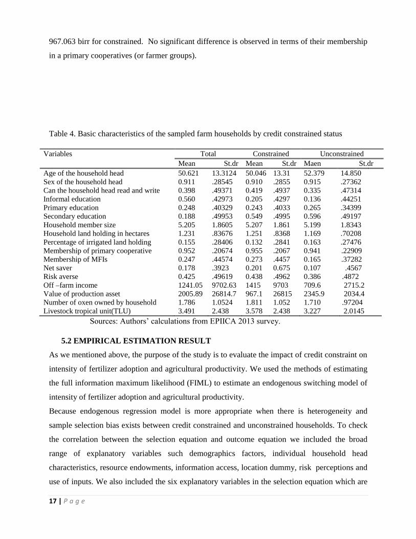
Table 4 below present some basic characteristics of sample households by classifying in credit

constrained and unconstrained regimes from EPIICA 2013 survey. There was no significant

difference in the age, land holding size, household member size and average education level

between constrained and unconstrained regimes. The average age of household head is round 51

years. And it is 50 and 52 years for credit constrained and unconstrained farm households,

respectively. This revealed that in both arrangements most householders are economically active

and able to effectively perform their agriculture. This shows that being other things remain

constant, there is a potential for improvement in farm income over the subsistence level.

The descriptive statistics shows that the majority of household heads are illiterate if some

householders who are able to write and read the acquisition by informal sectors and there are

some heads attending formal primary schools, secondary and upper secondary school in both

constrained and unconstrained regimes. From the total sample households 60% were illiterate.

Among literate household heads, 56% have attend informal education (religious, adult

education), 24.8% percent have primary education and 18.8 % have attend the secondary and

above education. The average land holding of the total sample household is 1.23 hectares. The

average land holding in constrained regimes was 1.25, while it was 1.16 hectares for

unconstrained households. It is also observed that credit unconstrained households have more

irrigated land (0.16%) than constrained households (0.13 %). This suggested that farm

households were mostly small scale producers in the region likewise in Ethiopia. In addition,

credit constrained households are more risk averse than unconstrained.

Surprisingly credit constrained households saved money more than unconstrained households.

This may be due to the reason that constrained households forced to save more afraid of risk and

smooth family consumption in the case of the credit market failure. Oxen are a very important

asset for rural households, because agriculture in Ethiopia depends on animal traction. On

average, both in the constrained and unconstrained regime households have two Oxen.

With regards to off-farm income, unconstrained households were earned less off-farm income

than constrained. On average, the farm households of the constrained regime were earned up to

1,414 birr a year, but, the households of the unconstrained regime gained up to 790 birr annually.

Credit unconstrained households have more the production of goods in Birr than their

counterpart. Value of production asset was 2345.928 birr in credit unconstrained regime, while

17 | P a g e

967.063 birr for constrained. No significant difference is observed in terms of their membership

in a primary cooperatives (or farmer groups).

Table 4. Basic characteristics of the sampled farm households by credit constrained status

Variables Total Constrained Unconstrained

Mean St.dr Mean St.dr Maen St.dr

Age of the household head 50.621 13.3124 50.046 13.31 52.379 14.850

Sex of the household head 0.911 .28545 0.910 .2855 0.915 .27362

Can the household head read and write 0.398 .49371 0.419 .4937 0.335 .47314

Informal education 0.560 .42973 0.205 .4297 0.136 .44251

Primary education 0.248 .40329 0.243 .4033 0.265 .34399

Secondary education 0.188 .49953 0.549 .4995 0.596 .49197

Household member size 5.205 1.8605 5.207 1.861 5.199 1.8343

Household land holding in hectares 1.231 .83676 1.251 .8368 1.169 .70208

Percentage of irrigated land holding 0.155 .28406 0.132 .2841 0.163 .27476

Membership of primary cooperative 0.952 .20674 0.955 .2067 0.941 .22909

Membership of MFIs 0.247 .44574 0.273 .4457 0.165 .37282

Net saver 0.178 .3923 0.201 0.675 0.107 .4567

Risk averse 0.425 .49619 0.438 .4962 0.386 .4872

Off –farm income 1241.05 9702.63 1415 9703 709.6 2715.2

Value of production asset 2005.89 26814.7 967.1 26815 2345.9 2034.4

Number of oxen owned by household 1.786 1.0524 1.811 1.052 1.710 .97204

Livestock tropical unit(TLU) 3.491 2.438 3.578 2.438 3.227 2.0145

Sources: Authors‟ calculations from EPIICA 2013 survey.

5.2 EMPIRICAL ESTIMATION RESULT

As we mentioned above, the purpose of the study is to evaluate the impact of credit constraint on

intensity of fertilizer adoption and agricultural productivity. We used the methods of estimating

the full information maximum likelihood (FIML) to estimate an endogenous switching model of

intensity of fertilizer adoption and agricultural productivity.

Because endogenous regression model is more appropriate when there is heterogeneity and

sample selection bias exists between credit constrained and unconstrained households. To check

the correlation between the selection equation and outcome equation we included the broad

range of explanatory variables such demographics factors, individual household head

characteristics, resource endowments, information access, location dummy, risk perceptions and

use of inputs. We also included the six explanatory variables in the selection equation which are

18 | P a g e

significantly determine the credit status of the households but weakly affect the intensity of

fertilizer adoption and productivity.

5.2.1 Determinants of credit constraints

In this section, we focus on the determinants of credit constraints in the selection equation. As it

has been defined above credit constrained is an excess demand and farm household unable to

borrow because of unfavorable credit conditions includes afraid of risk, required collateral too

high, high interest rate, high transaction cost and loan process is much time consuming. Credit

constraint is treated as binary outcome model, leveled the value “1” if the household being credit

constrained and leveled the value “0” otherwise. In table 5 below the selection equation

estimation presents the factors which affect the farm households‟ probability of undergoing the

credit constraint. The selection model result is derived from running probit regression within

endogenous switching regressions for a dichotomous choice of being credit constrained. The

selection equation includes the all explanatory variables from the intensity of fertilizer adoption

and agricultural productivity as well as membership of MFIs, borrowing interest rate, bank

account dummy, bank trust dummy, Muslim headed dummy and number of installments were

administrate as set of instrumental variables that will strongly affect the credit status but

weakly/not the intensity of fertilizer adoption and, agricultural productivity.

The result for selection equation (credit constrained) from table 5 and 6 show that age of

household head have non-linear relationship with the households‟ probability of being credit

constrained. Age of the household head has the negative and significant effect on credit

constraint while, age square has positive and significant. This implies initially when age increase

it minimize the credit constraint, and then when household head become old age, household is

more likely to face a credit constraint problems. Here we can understand that the households

who have old age household head face credit constrained problems than the households who

have young age household head. The possible reason for the nonlinear effect of age on the credit

constraint because of the reason that younger farms are more productive and physical capable to

their production scale expands, and more and more capital is required to fulfill their production

inputs. When those farm owners enter their middle age, most farm operators maximize their

production investment. Therefore, middle-age farm operators have higher probabilities of being

credit constrained. This possibility decreases as they become older, when their interest in the

19 | P a g e

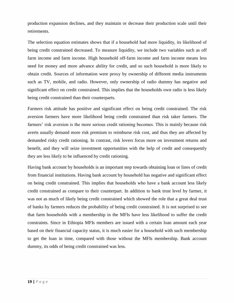
production expansion declines, and they maintain or decrease their production scale until their

retirements.

The selection equation estimates shows that if a household had more liquidity, its likelihood of

being credit constrained decreased. To measure liquidity, we include two variables such as off

farm income and farm income. High household off-farm income and farm income means less

need for money and more advance ability for credit, and so such household is more likely to

obtain credit. Sources of information were proxy by ownership of different media instruments

such as TV, mobile, and radio. However, only ownership of radio dummy has negative and

significant effect on credit constrained. This implies that the households own radio is less likely

being credit constrained than their counterparts.

Farmers risk attitude has positive and significant effect on being credit constrained. The risk

aversion farmers have more likelihood being credit constrained than risk taker farmers. The

farmers‟ risk aversion is the more serious credit rationing becomes. This is mainly because risk

averts usually demand more risk premium to reimburse risk cost, and thus they are affected by

demanded risky credit rationing. In contrast, risk lovers focus more on investment returns and

benefit, and they will seize investment opportunities with the help of credit and consequently

they are less likely to be influenced by credit rationing.

Having bank account by households is an important step towards obtaining loan or lines of credit

from financial institutions. Having bank account by household has negative and significant effect

on being credit constrained. This implies that households who have a bank account less likely

credit constrained as compare to their counterpart. In addition to bank trust level by farmer, it

was not as much of likely being credit constrained which showed the role that a great deal trust

of banks by farmers reduces the probability of being credit constrained. It is not surprised to see

that farm households with a membership in the MFIs have less likelihood to suffer the credit

constraints. Since in Ethiopia MFIs members are issued with a certain loan amount each year

based on their financial capacity status, it is much easier for a household with such membership

to get the loan in time, compared with those without the MFIs membership. Bank account

dummy, its odds of being credit constrained was less.

20 | P a g e

5.2.2 Impact of Credit Constrained on of intensity of fertilizer adoption

The objective of the study to compare the diverse extent of fertilizer adoption between credits

constrained and unconstrained smallholder farmers, under imperfect credit market in Amhara

region, Ethiopia. Table 5 below present results from switching regression model for intensity of

fertilizer adoption. In this study, we include various farm characteristics variables, resources

endowment and institutional factors which are theoretically associated with the intensity of

fertilizer adoption. The dependent variable is logarithm of intensity of fertilizer adoption by

smallholder farmers. The intensity of fertilizer adoption is defined quantity of fertilizer used (in

Kg) divided by total area of land (in hectare) cultivated by farmers.

The correlation coefficient roh_1 indicates the correlation between the credits constrained

situation and the effects of credit constraint on intensity of fertilizer adoption by credit

constrained households. The estimated result is negative and significant. The value is 0.17 which

is a very strong correlation, the implication that being credit constrained has significant adverse

effect on intensity of fertilizer adoption. Thus, the individuals that were credit constrained used

smaller fertilizer in their farming than a random individual from the sample would have. The

correlation coefficient roh_2 indicates the correlation between the credit constrained situation

and the effects of credit constraint on intensity of fertilizer adoption by credit unconstrained

households. The value is positive and statically significant. The value is 0.24 which is a very

strong correlation. This implies that those who were credit unconstrained used more fertilizer in

their farming than a random individual from the sample would have. The likelihood-ratio test for

joint independence of the three equations reported in the last row of table 5 showed that these

three models are not jointly independent and should not be estimated separately.

As we observe from the table 5 below the result is diverse across credit constrained and

unconstrained regime. The estimation result demonstrate that age of the household head has

positive and significant effect on the intensity of fertilizer adoption in unconstrained regime,

while age square of the household head has a negative and significant on the intensity of

fertilizer adoption in unconstrained regime . This implies that age of the household head is not

linearly correlated with intensity of fertilizer adoption. The result could be explained that

younger people may be more adaptive and more willing than older people to try new methods

like fertilizer and use more fertilizer to expand their production when they are credit

unconstrained. However, both age and age square of household age have no significant effect on

21 | P a g e

the intensity of fertilizer adoption in constrained regime. The household size had a positive and

significant effect on the intensity of fertilizer adoption in the credit constrained regime but it had

no effect on the intensity of fertilizer adoption in the unconstrained regime.

The result indicate that households‟ membership in primary cooperatives happen to determine

the intensity of fertilizer adoption used positively and significantly in the credit unconstrained

regime however, it had no significant effect on the intensity of fertilizer adoption in the

constrained regime. The prior expectation is that as farmers belong to primary farm cooperatives

they learn from others, and thus they will have access to information which enhances the

adoption of new agricultural practices. Heterogeneity effect of primary cooperative membership

on intensity of fertilizer adoption among credit constrained and unconstrained regime can be

explained by the fact that once the decisions to adopt fertilizer may be made based on the

availability of information, the intensity of fertilizer adoption will depend on the ability of the

farmer households to finance price of fertilizer from own resources and accessibility of credit.

This implies that the effect of primary cooperatives membership on intensity fertilizer adoption

is condition with the credit accessibility.

In this study, education of the household head is categorized into three informal, primary and

secondary education. To avoid multicollinearity problem we used informal education as base

dummy. The estimation result suggested that both primary and secondary education dummy has

a positive and significant effect on intensity of fertilizer adoption in both regimes. The result can

be explained that education may facilitate fertilizer use by improving access to information on

and knowledge of fertilizer.

The financial liquidity availability is an important determinant of fertilizer use. In this study

financial liquidity is measured by two variables such as off-farm income and farm income.

Because off-farm income can a substitute for borrowed capital in rural economies where credit

markets are imperfect. The regression result shows that off farm income has a positive but

insignificant outcome on the intensity fertilizer adoption in both credit constrained and

unconstrained regime. On the other hand the result shows that higher farm income had

significantly promote the intensity of fertilizer adoption. The implication of the result is that

intensity of fertilizer adoption decisions are significantly affected by a marginal change in farm

income. Because farmers use additional liquidity to invest farm production like purchased

fertilizer and other complementary inputs. The value of production assets which was used as a

22 | P a g e

proxy for household wealth had a positive and significant effect on the intensity of fertilizer

adoption in the credit constrained regime but it had no effect on the intensity of fertilizer

adoption in the unconstrained regime.

Land holding size has negative and significant effect on the intensity of fertilizer adoption in the

credit constrained regime, implying that per hectare fertilizer use decreases as farm size

increased. While, it had a positive and significant effect on the intensity of fertilizer adoption in

the unconstrained regime. The result is consistent with the study by Weil (1970) the negative

relationship between intensity of fertilizer adoption and land holding size may be caused by

credit constraints. The positive effect of land holding size can be explained by capital may be

more available for larger farms, so that even though all farms may wish to adopt, larger farms are

more likely to do so. Thus, households with larger holdings are also likely to be wealthier, with

increased ability for self-financing the purchasing of inputs and they have better probability to

get credit as compare to smaller farmers.

With respect to percentage of irrigated land, the coefficient is positive and statistically significant

in both the credit unconstrained and constrained regimes. The result is not surprising because

firstly, irrigation enables crops to absorb more fertilizer, which motivates farmers to apply a

greater quantity if no binding credit constraints or shortage of financial asset to finance the

fertilizer price. Secondly, irrigated land has more protected yields under the situation of

unpredictable rainfall, thus farmers face lower risks when applying the fertilizer more

intensively. Average slope of land, average altitude of land and average ownership of land are

significant and positive determinants of intensity of fertilizer adoption in the credit constrained

regime whereas none of these variable are significant in the credit unconstrained regime.

Source of information is cited as an important determinant of fertilizer adoption and intensity of

fertilizer adoption. Here source of information is proxy by ownership of Mobile, TV, and Radio.

As we can see from the result ownership of mobile and TV had found the significant and positive

determinants of intensity of fertilizer adoption in the credit unconstrained regime, however, only

ownership of mobile dummy is positive and significant in the credit constrained regime. This

provides the evidence that farmers who have own TV and Mobile may have better information

on the use of fertilizer and new agricultural practice than their counter part, especially if there is

no extension services in the area.

23 | P a g e

Farmers‟ risk attitudes determine farmers‟ intensity of fertilizer adoption and the consequences.

The risk aversion dummy is significant and positive on the intensity of fertilizer adoption in the

constrained regime, while it has no such effect on intensity of fertilizer adoption in credit

unconstrained regime. This heterogeneity effect may arise because credit constrained farmers

will use fertilizer more intensively to increase their production, meet households needs and to

avoid future consumption risks. The result may not be surprised to have negative and significant

coefficient of manure in the extent of fertilizer adoption for both credit constrained and

unconstrained farmers. This implies that manure plays an important role in farmers‟ decision

making and generally offsets the use of chemical fertilizers. In fact inorganic fertilizer and

manure are substitute inputs. Thus, farm households that have and apply sufficient quantities of

manure would not require more chemical fertilizer.

Table.5Parameters Estimates of credit rationing and fertilizer use intensity

Constrained Unconstrained Selection(credit status)

Coef Std.err Coef Std.err Coef Std.err

Male headed dummy -0.139 0.235 -0.067 0.144 0.162 0.120

Marital status 0.163 0.209 -0.096 0.130 0.097 0.109

Log of Age of the household head 31.892 45.475 57.919* 26.253 51.518* 22.077

Log of Age square of the household

head

15.676 22.255 -28.214* 12.844

-25.149* 10.803

Log Household size -.2675* 0.130 -0.082 0.075 .163 0.064

Primary education dummy .457** 0.146 .357*** 0.077 -0.046 0.071

secondary education dummy .425*** 0.125 .439** 0.071 0.026 0.067

Primary cooperative membership

dummy

-0.198 0.167 .362*** 0.093

-0.063 0.081

Livestock ownership in TLU -0.019 0.138 -0.102 0.075 -0.003 0.010

Log of number of ox 0.234 0.153 .329*** 0.003 -0.148 0.078

Log of Off- farm income 0.035 0.021 0.019 0.010 -0.093*** 0.015

Log of Farm income .067** 0.023 .098*** 0.014 -0.078*** 0.012

Log of value production asset .1397* 0.058 0.031 0.030 -0.028 0.027

Ownership of TV dummy -0.289 0.256 .399** 0.132 -0.066 0.124

Ownership of mobile dummy .188* 0.088 .118** 0.041 -0.078 0.040

Ownership of radio dummy -0.175 0.112 0.084 0.057 -.108* 0.052

Hired labor dummy 0.192 0.108 .1405* 0.061 0.098 0.053

Average slope index (1 all parcel

steeply sloped, 3 all flat)

0.184 0.097 -0.105 0.054

-0.058 0.047

Average altitude index( 1=all parcel

much above 5=all much below

.1674** 0.054 -0.002 0.034

-0.019 0.028

Average land ownership index(1=all

parcel fully owned by hh 4= all

rented)

.207*** 0.060 0.043 0.029

-0.021 0.027

Ways of land cultivation .775** 0.270 0.240 0.164 -0.084 0.138

Average distance of parcel from home -0.004 0.002 -0.001 0.001 .0038*** 0.001

Log of parcel in hectare -.1566*** 0.037 .2710*** 0.022 -0.031 0.019

Percentage of irrigated land .906*** 0.204 .973*** 0.098 -.239** 0.090

24 | P a g e

log of manure used -0.010 0.017 -.043*** 0.009 0.002 0.008

Dummy for households in North Wello -.5023** 0.163 -

.4246***

0.087 -.5023** 0.163

Dummy for households in south Wello -.560*** 0.130 -.408*** 0.074 -.560*** 0.130

Dummy for households in W/Gojjam 2.449*** 0.124 2.267*** 0.073 2.449*** 0.124

Risk averse household dummy 1.0337*** 0.2648 -0.0133 0.0863 0.3650*** 0.0858

Membership of MFIs -.427*** 0.064

Borrowing interest rate .0190*** 0.0047

Bank account dummy -.258*** 0.066

Bank trust dummy -0.042 0.052

Muslim headed dummy -0.1571 0.086

Number of installments 0.0007 0.014

cons. 1.359 4.948 8.64** -5.966* 2.397

lns1 0.320*** 0.0387

lns2 0.322*** 0.0124

r1 -0.181 0.251

r2 0.083762 .

sigma_1 1.377 0.053

sigma_2 1.3799 0.0171

rho_1 -0.1797 0.2429

rho_2 0.083567 .

LRtestchi2(1)=80.2Prob=0.000

chi2 = 0

Statistical significance at the 99% (***), 95% (**) and 90% (*) confidence levels.

5.2.3 Average fertilizer used intensity: treatment and heterogeneity effect

Table 6 below presents the expected value of intensity of fertilizer adoption under actual and

counterfactual conditions. From the table, Cell (A) and (B) defined the expected value of

intensity of fertilizer adoption observed in the sample. The expected value of intensity of

fertilizer adoption by credit unconstrained households is higher than credit constrained

households. This simple comparison between the observed mean values however, can be

misleading and drive the researcher to conclude that on average the intensity of fertilizer

adoption by credit unconstrained farmers is higher than for credit constrained farmers. To avoid

this problem we used the counterfactual analysis. It can be by subtracting cell (C) from cell (A).

The result from the table 6 indicate that mean intensity of fertilizer adoption would be higher if

they are credit unconstrained. Average treatment effect(ATT) result shows that credit

constrained households would have used about 42Kg fertilizer per hectares( 54%) less than if

they had credit unconstrained. Similarly, ATU can be calculated by subtracting cell (D) from cell

(B). The ATU value of (1.51Kg) implies that unconstrained households would have used about

1.51 kg fertilizers per hectares more than if they had credit constraints. These results imply that

access to credit could increase intensity of fertilizer adoption. The transitional heterogeneity

25 | P a g e

effect is negative(-41.361), this evidence that access to credit has smaller effect for the farm

household that actually credit constrained with respect to those that credit unconstrained.

Table 6. Average expected intensity of fertilizer adoption per hectares for credit constrained and

unconstrained households.

Sub-sample Decision Stage

Constrained Unconstrained Treatment Effects

Households being

credit constrained

49.151(A) 91.022(C) -41.871 (ATT)

Households being

credit unconstrained

57.45(D) 58.96 (B) 1.51(ATU)

Heterogeneity effects 8.299 32.062 -41.361

5.2.4 Impact of Credit Constrained on productivity

Table 7 below reports the repressors estimated parameter used in the both the agriculture

productivity per hectare (as continuous variable) and selection equation (credit constrained

equation). The result revealed that for credit unconstrained farm households, productivity is

increasing in the age of households head, while it decreasing in the age square. This implies that

households with older household heads had lower productivity than those with younger

household heads. On another hand both age and age square of household head have no

significant effect on farm productivity in constrained regime. The result confirmed that younger

farmers had higher productivity and get higher farm income when they are credit unconstrained.

Agricultural production in Amhara region as well in Ethiopia is mostly labor intensive. Only

without credit constraints can younger farmers make full use of their physical advantage.

Various literatures quoted education of household head is important determinant of the

households‟ farm productivity. As stated above, education is categorized into three levels:

informal education, primary education and secondary education. The variable informal education

is used as the base and deleted from the regression to avoid singularity or multicollinearity

problems. The result revealed primary education and secondary education dummy variable is

positively and significantly affect household‟s productivity in both constrained and

unconstrained regime.

Total cultivated land had found significant and positive effect on productivity for unconstrained.

This implies that farmers with more land likely to increase productivity when they are credit

unconstrained. The result can be explained large scale farmers are less risk averse and more

inclined to make agricultural investment than small scale farmers and thus they can increase their

26 | P a g e

productivity. Moreover, the positive correlation between farm size and productivity may arise

from the economies of scale in acquiring information and getting input credit. However,

cultivated land size is negative and significant for constrained. This indicating that credit

constrained farmers with more land are unlikely to increase productivity. The negative effect of

farm size on the productivity is consistent with the literature (Feder et.al., 1985; Martey et al.,

2013) indicated that management labor, required finance to purchase fertilizer and improved

seed or other constraints limit the ability of larger farmers to be as productive and generate large

income as smaller farmers. This problem serious particularly when the farmers are credit

constrained. Regarding the percentage of irrigation land, it is significant and positive for both

constrained and unconstrained regimes.

In fact geographic location of farms determines cropping pattern, rainfall amounts, soil

productivity, access to market and access to different institutional services. In order to examine

the effect of geographic location variation among farmers on farm income we used three location

dummy (such as North Wello, south Wello and Gojjam to represent farmer‟s location and used

north Shewa as base dummy and deleted from the regression to avoid singularity problem. The

estimated result shows that South Wello had a positive and significant effect on productivity in

both constrained and unconstrained regimes. This result confirms that South Wello farms were

more likely to increased productivity as compared to farms in the North Shewa. The result is

surprising because farmers in South Wello frequently affected by drought and the land less fertile

as compare to North Shewa. This kind of result may arise because if the farmer frequently faced

risk and their land less fertile they will made diverse activities and used land more intensively to

meet subsistence needs. The North Wello dummy is significant negative in the unconstrained

regime, while it is negative insignificant in the constrained regime. The result revealed that farm

in North Wello unlikely to increased productivity as compare to farms in North Shewa. The

result may be explained by productivity difference between two zones. North Wello zone is one

of the degraded and less productive areas in the country and suffered with frequent drought. All

these factors create unfavorable conditions for the farmer to increase agriculture productivity and

thereby increase welfare.

The total livestock asset is measured using tropical livestock unit. It is significantly positive for

unconstrained, but insignificantly positive for constrained. The result revealed that ownership of

livestock would increase farm productivity. The number of oxen owned by households is also

27 | P a g e

positively significant in credit constrained regime. The result may be explained various ways: if

the households who have more livestock, they may finance input cost by selling their livestock

and thus increase the productivity as well farm income. On other hand, in fact crop production

in Ethiopia is dependent on animal traction therefore farmers with more livestock they could be

increase crop production and their income.

Based on the literatures the effect of off-farm income on household‟s farm productivity is

ambiguous. Off-farm income is a substitute for borrowed capital in rural economies where credit

markets are either missing or dysfunctional. In other word off-farm income relaxed financial

constraints by farmer which is required to purchase productivity enhancing inputs such as

improved seed and fertilizers (Mary K. Mathenge and David L. Tschirley 2009). On the other

hand, pursuit of off-farm income by farmers, higher return off-farm income and less risky nature

may undermine farm activity. In this particular study off- farm income had a significant and

negative effect on the productivity in both credits constrained and unconstrained regimes. This

implies that as off-farm income increased could leads to decrease in farm productivity and farm

income.

Table 7. Parameters Estimates of credit constraints and Farm productivity

Explanatory Constrained Unconstrained Selection equation

Coef Std.err. Coef Std.err. Coef Std.err.

Male headed dummy -0.008 0.311 -0.127 0.177 0.162 0.120

Marital status 0.260 0.277 -0.002 0.159 0.100 0.108

Log of Age of the household head -61.528 60.165 89.183** 32.622 52.218* 22.126

Log of Age square of the household head 30.006 29.444 -43.50** 15.959 -25.49* 10.827

Log Household size -0.322 0.171 0.002 0.092 .160* 0.064

Primary education dummy .852*** 0.192 -0.169 0.095 -0.051 0.071

Secondary education dummy .928*** 0.161 -.528*** 0.087 0.056 0.062

Primary cooperative membership dummy -0.172 0.220 0.193 0.114 -0.062 0.081

Livestock ownership in TLU 0.142 0.182 .319*** 0.092 -.1459* 0.066

Log of number of ox .544** 0.203 0.141 0.112 -0.142 0.078

Log of Off- farm income -.0609* 0.027 -.0325* 0.013 -0.004 0.010

Log of value production asset .1397* 0.058 0.031 0.030 -0.022 0.027

Ownership of TV dummy 0.483 0.340 0.294 0.162 -0.059 0.124

Ownership of mobile dummy .283* 0.115 0.069 0.051 -0.075 0.040

Ownership of radio dummy -0.107 0.148 -0.114 0.071 -.1108* 0.052

Hired labor dummy 0.093 0.142 .291*** 0.075 0.101 0.053

Average slope index (1 all parcel steeply sloped, 3 all

flat)

-0.151 0.129 0.011 0.067

-0.058 0.047

Average altitude index 1 all parcel much above 5 fall

much below)

0.073 0.071 -0.051 0.042

-0.020 0.028

Average land ownership index(1all parcel fully

owned by hh 4 all rented)

0.004 0.079 0.044 0.036

-0.020 0.027

28 | P a g e

Ways of land cultivation 0.502 0.357 0.119 0.201 -0.082 0.139

Average distance of parcel from home -.0052* 0.002 0.001 0.002 .0038*** 0.001

Log of parcel in hectare -.1575** 0.049 .3516*** 0.026 -0.028 0.019

Percentage of irrigated land 1.756*** 0.259 1.212*** 0.120 -.215* 0.088

Log of chemical fertilizer used in kg .0678*** 0.047 .1082*** 0.022 -.051*** 0.016

log of manure used in kg -0.026 0.022 -0.007 0.011 0.002 0.008

Use of improved seed dummy .322*** 0.164 .243*** .080 .1128 0.059

Dummy for households in W/Gojjam 0.008 0.164 -0.004 0.090 -0.110 0.066

Dummy for households in south Wello .431* 0.171 .252** 0.092 -0.033 0.093

Dummy for households in North Wello -0.385 0.217 -.5768*** 0.109 -.2097** 0.076

Membership of MFIs -.424*** 0.062

Borrowing interest rate .0191*** 0.004

Bank account dummy -.259*** 0.067

Bank trust dummy -0.048 0.054

Muslim headed dummy -0.153 0.084

Number of installments 0.001 0.015

_cons 15.031* 6.516 -3.246 3.551 -5.922* 2.402

lns1 0.595*** 0.023

lns2 0.523*** 0.012

r1 -0.046 0.240

r2 0.027 0.121

sigma_1 1.814 0.041

sigma_2 1.688 0.021

rho_1 -0.046 0.239

rho_2 0.027 0.121

LR test of indep. Eqns. chi2 (1) = 61.63 Prob> chi2 = 0.0000

Statistical significance at the 99% (***), 95% (**) and 90% (*) confidence levels.

5.2.5 Average farm productivity: Treatment and Heterogeneity effect

The results discussed above suggest that household resource allocation and productivity is

affected by credit constraints. In addition to these we also need to estimate the magnitude of how

much productivity would increase if the credit constraints were removed. Table 8 below shows

that the results of counterfactual analysis using the estimates from endogenous switching

regression to calculate the actual (observed) and counterfactual productivity for both credit

constrained and unconstrained households as well as to compute the productivity loss due to

credit constraints. From table 8 Cell (A) and (B) defined the expected value of productivity

observed in the sample. As we shown from the result the expected productivity for credit

constrained is higher than unconstrained. However, ATT result indicates that if the credit

constraints were removed, mean household productivity could be increased by 6571. 28 birr

which is about 18.85% increase. ATU is result revealed that productivity for credit unconstrained

households could be decreased by 5689.8(16.83%) birr if they had credit constrained. The

transitional heterogeneity effect is negative; this shows that access to credit has smaller effect for

29 | P a g e

the farm household that actually credit constrained with respect to those that credit

unconstrained.

Table 8. Average expected productivity per hectares for credit constrained and unconstrained

households.

Sub-ample Decision Stage

Constrained Unconstrained Treatment Effects

Households being credit

constrained

38986.72(A) 45558(C) -6571. 28

Households being credit

unconstrained

28102.12(D) 33791.92(B) 5689.805

Heterogeneity effects 1884.6 11766.08 -881. 475

Sources: author‟s calculation 2016.

6. Conclusion and Policy Implication

The development of financial sectors and their products have been identified as a means to

facilitate the adoption of farm inputs and boost agricultural productivity in Ethiopia as well as in

developing countries. In Ethiopia, however, the smallholder farmers are still credit rationed.

Many of economic theory argued that providing credit at market interest rate will leads to the

marginal benefit among the credit constrained households while, does no welfare enhancement

effect for the unconstrained households. Therefore, intensifying technology adoption, boosting

agricultural productivity and alleviating poverty in rural area in credit allocation require targeting

the credit constrained households. The main objective of the study is to examine the impact of

credit constraint on intensity of fertilizer adoption and agriculture productivity among household

that vary in the credit constraint status.

The study was utilized a cross sectional farm household data collected in 2013 from randomly

selected sample of 1165 in Amhara region, Ethiopia. With the data, an endogenous switching

regression is applied because it taking into accounts the endogneity problems of credit

constrained and intensity of fertilizer adoption and credit constrained status and agricultural

productivity.

We find that credit constraints negatively associated with age of the household head, liquidity,

ownership of radio, percentage of irrigated land, bank account and location dummy includes(

North Wello and South Wello) but, positively associated with interest rate, risk averse , land

distance from home and location dummy of Gojjam. Our result confirmed that factors have a

different impact on the intensity of fertilizer adoption and agricultural productivity among credit

30 | P a g e

constrained and unconstrained households. For, example, while age and age square of the

household head had a non –linear and significant effect on intensity of fertilizer adoption in the

unconstrained regime, it had no effect among constrained households. The effect of land size on

extent adoption is also a variable with an opposite effect between the two regimes. Results

indicated that while larger land holdings lead to used more mount of fertilizer in the

unconstrained regime, it has a negative effect on extent of fertilizer adoption in the constrained

regime maybe due to credit constraints.

Moreover, the result shows that intensity of fertilizer adoption for credit constrained households

are affected by several factors such as primary cooperative membership, number of oxen source

of information includes ownership of TV and mobile phone, percentage of irrigated land and

hired labor, use of manure and location dummy (North Wello and South Wello), while household

size and land property (include altitude of land, ownership of land, way of land cultivation,

percentage of irrigated land), Gojjam dummy and risk averse are important for intensity of

fertilizer adoption of constrained households, implying that credit constraint status has made the

significant in the intensity of fertilizer adoption.

Agriculture productivity associated with that Age and age square of the household head, TLU,

hired labor dummy are the factors significantly affect the productivity in the unconstrained

regimes. While number oxen, distance of land from home are significantly affect the agricultural

productivity in the constrained. Land size has found the significant and negative effect on the

productivity in the constrained regime but, it has the positive and significant effect in the credit

constrained regime.

We also conducted the counterfactual analysis with the endogenous switching regressions and

estimated the actual and counterfactual extent of fertilizer adoption and agricultural productivity

for both credit constrained and unconstrained households in order to explicitly measure the

impact of credit constraints. And the result shows that extent of fertilizer adoption would be

decline by 55 kg per hectares if unconstrained households will be constrained. On the other

hand, constrained are estimated to increase their intensity of fertilizer adoption by 33% if they

are unconstrained.

Similarly, the counterfactual analysis between agricultural productivity and the credit

constrained status revealed that agricultural productivity would be decreased by 16.83percent if

31 | P a g e

unconstrained farm household will be constrained. Agriculture productivity would be increased

by 16.85 percent if constrained farm households were unconstrained. The fact credit constrained

higher impact on the intensity of fertilizer adoption and productivity among the credit

constrained and unconstrained farm households justifies the need for credit targeting to boost the

agricultural productivity and it can have far reaching poverty reduction implication especially in

rural areas farming is the major source of income and food production. Therefore, provision of

credit to poor with the market interest rate is a sound policy instrument to raise income of farm

households and fight against poverty in the rural area. The policy implication is that the policy

maker should account the credit constraint heterogeneity among farm households, when they

design agricultural policy to increased intensity of fertilizer adoption and thereby boost

productivity.

7. Reference

Agriculture Finance Support Facility (AGRIFIN) (2012) technical brief summarizes the Enabling

Environment: Access to Financial Services and Transportation chapter of the World Bank report on

Agribusiness Indicators: Ethiopia

Assefa Admassie, (2004) A Review of the Performance of Agricultural Finance in Ethiopia: Pre

and Post- Reform Periods

CSA (Central Statistic Authority), (2014) Agricultural Sample Survey, Volume I - Report on Area

and Production Crops, Addis Ababa

Daniel Ayalew Ali and Klaus Deininger, (2012) Causes and Implications of Credit Rationing in

Rural Ethiopia: The Importance of Spatial Variation. The World Bank Policy Research

Working Paper 6096

De Janvry A. Murgai, R. and Sadoulet E., (1999) Rural Development and Rural Policy,

University of California at Berkeley and the World Bank.

Diagne, A. & Zeller, M., (2001) Access to credit and its impact on welfare in Malawi,

Washington, D.C.: IFPRI

Dutoit, Laure. (2007) Hickman Selection Model, Endogenous and Exogenous Switching Models:

A Survey. Unpublished, University of Lausanne. http://works.bepr ess.com/laure_dutoit/3/

Feder, G., Lau, L. J., Lin, J. Y., & Luo, X. (1989) Agricultural Credit and Farm Performance in

China. Journal of Comparative Economics 13 (4)

32 | P a g e

Feder, G., Lau, L. J., Lin, J. Y., & Luo, X., (1990) the Relationship between Credit and

Productivity in Chinese Agricultural: A Microeconomic Model of Disequilibrium. American

Journal Agricultural Economics Vol. 72 (5)

Feder, Gershon & Just, Richard E &Zilberman, David. (1985) " Adoption of Agricultural

Innovations in Developing Countries: A Survey. Economic Development and Cultural

Change, 33(2), 255-298

Girma and Abebaw (2015) Determinants of Formal Credit Market Participation by Rural Farm

Households: Micro-level evidence from Ethiopia: Paper for presentation at the 13th

International Conference on the Ethiopian Economy. Ethiopian Economic Association (EEA)

Conference Centre, Addis Ababa, Ethiopia, July 23-25, 2015

Imoudu P.B. and E. Onaksaponome (1992) “Bank Loan Requirement and Availability for

Nigerian Small Farmers – A comparative Analysis of Experience. FINAFRICA, African

Review of Money Finance and Banking, 1: 49-61.

Jeffrey M. Wooldridge (2010) Econometric Analysis of Cross Section and Panel Data The MIT

Press Cambridge, Massachusetts , London, England

Kyriazidou, E. (1997). Estimation of a panel data sample selection model. Econometrica,

65:1335–1364.

Lokshin, M., Sajaia, Z., (2004) “Maximum Likelihood Estimation of Endogenous Switching

Regression Models.” The Stata Journal 4(3): 282-289.

Maddala GS (1983) Limited-Dependent and Qualitative Variables in Econometrics, New York

Cambridge University Press,

Martey, E. , Nimo, A., Wiredu Prince M. Etwire, Fosu M., S. S. J. Buah, Bidzakin,J Benjamin D.

K. Ahiabor&Kusi,F. (2013) Fertilizer Adoption and Use Intensity Among Smallholder

Farmers in Northern Ghana: A Case Study of the AGRA Soil Health Project

Mary K. Mathenge and David L. Tschirley (2009) off farm work and farm production decisions:

evidence from maize producing households in rural Kenya, Teemed Institute of Agricultural

Policy &Development Kindaruma Lane, off Ngong Road press, WPS 33/2008

McIntosh et.al (2013) Productivity, credit, risk, and the demand for weather index insurance in

smallholder agriculture in Ethiopia, Agricultural Economics 44 (2013) 399–417

MOA (2010) Ethiopia‟s Agriculture Sector Policy and Investment Framework (PIF) 2010-2020,

Final Draft Report.

33 | P a g e

Nin-Pratt, A. & Yu, B. (2010). Agricultural Productivity and Policy Changes in sub-Saharan

Africa. USDA Economic Research Service, 1800 M St NW, Washington DC 20036

Ogato, G., Boon, E. & Subramani, J. (2009) Improving access to productive resources and

agricultural services through gender empowerment: A case study of three rural communities in

Ambo District, Ethiopia. Journal of Human Ecology, 27, 85-100.

UNDP(2015) ETHIOPIA: Key Economic and Social Indicators

USAID (2008) common problems in impact assessment research: impact assessment primer

series publication NO. 7

Weil, P.M. (1970). The Introduction of the Ox Plow in Central Gambia, Mclaughlin, P.F. (Eds.)

(1970) African Food Production Systems: Cases and Theory, Baltimore, John Hopkins

University Press.

Zerfu, D., Larson, D.F., (2010). Incomplete markets and fertilizer use: Evidence from Ethiopia.

World