Effect of Bond Strength on Performance of Pavement

International Journal of Advance Research in Engineering, Science & Technology(IJAREST),

ISSN(O):2393-9877, ISSN(P): 2394-2444, Volume 2, Issue 6, June- 2015, Impact Factor: 2.125

55

All Rights Reserved, @IJAREST-2015

Effect of Bond Strength on Performance of Pavement

Suhas.S.Biradar, Avinash.Angadi, Pradeep.Yaragatti,Hanmantarao.G.Joteppanavar 1Civil Engineering, KLE Dr.M.S.Sheshgiri college of Engineering & Technology,Belgaum,[email protected]

2Civil Engineering, KLE Dr.M.S.Sheshgiri college of Engineering & Technology,Belgaum,[email protected]



Abstract

A mechanistic model of flexible pavement was considered and constructed to study the effects of shear modulus on performance of

various pavement layers. The objective of this study was to quantify the effects of interlayer bonding by varying of the shear modulus

of the contact layer. Flexible pavements are complex structures consisting of several layers of asphalt and granular materials .

Bonding is assessed due to increase or decrease of critical stress values when static loading condition is maintained with constant

elastic properties such as Modulus of elasticity, shear modulus etc. The flexible pavement works as a single structure due to good

bonding between the different layers. Lack of bonding destroy continuity, decrease structural strength, and allow water to enter sub

layers. Bituminous tack coat is laid to ensure contact of the aggregates of the various layers of the flexible pavement. The viscous

nature of the flexible pavement, allows its different layers to sustain significant plastic deformation, although distresses due to

repeated heavy loading over time which is the most common failure mechanism. It is generally believed that, the pavement stress

distribution is extremely influenced by the adhesion conditions at the layer interface .This characteristic is used to access pavement

performance.

Keywords—Adhesion, Bonding, Critical stress, Elastic Modulus, Shear Modulus, Flexible pavement ,Finite Element analysis,

Static wheel load, Multiple regression analysis

I. INTRODUCTION

The viscous nature of the flexible pavement, allows its

different layers to sustain significant plastic deformation,

although distresses due to repeated heavy loading over time

which is the most common failure mechanism.

Poor adhesion at layer interface may cause adverse effects on

the structural strength of the pavement system and form

numbers of premature failures. To increase bonding between

layers, bituminous tack coats are applied prior to overlay.

Bituminous emulsions are normally used as tack coats. In spite

of their extensive application, the thoughts among pavement

engineers differ regarding the effectiveness of tack coat in

enhancing the adhesion between the two layers. This tack coat

also made of a thin layer of bitumen residue and its objective

is to provide adequate adherence between the layers. If the

quantity of bituminous emulsions used is in excess or less than

the required one, the interface bonding will not be satisfactory.

One assumption in the structural response model for flexible

pavements is that the asphalt layers and completely bonded to

each other, when in all reality they may not be[1]. There is no

widely accepted test method for measuring the degree of

bonding between pavement layers. Without proper modeling

of the bond between layers, the calculation of pavement

response, and thus the design of the flexible pavement

structures, cannot be accurate. Poor bonding between

pavement layers can cause many distresses[2]. One of the

most common distress is slippage failure, which usually

occurs where heavy vehicles are often accelerating,

decelerating, or turning. Being a layered structure, the life of

an asphalt pavement not only depends on the strength and

stiffness of its individual layers, but also on the bond between

them. The bonding characteristics are mainly influenced by

the bond strength analysis of the flexible pavement layers

which is mainly influenced on elastic properties such as

modulus of elasticity, shear modulus, poison's ratio etc. The

present work involves accessing of the effect of the bond

strength on the performance of pavement as a elastic body by

the stresses induced in the individual layers due to the effect of

loading and elastic properties[3]. The increasing values of the

critical stresses indicate poor bonding while the decreasing

value of stresses indicate better bonding causing elastic

deformation at the surface of the pavement as the effect of

load transfer from layer to layer.

Present work involves determination of the relation between

the elastic properties on the bond strength of the pavement by

performing multilayer regression analysis. The bonding is

accessed by introduction of a contact layer in the five layered

flexible pavement whose shear modulus has the influence on

the bonding characteristics. The analysis is done with a finite

element approach of the flexible pavement by developing a

mechanistic model in Ansys APDL with assigning of material

properties i.e. modulus of elasticity ,shear/rigidity modulus

and poison's ratio. Various models analyzed varying modulus

of elasticity for sub grade sub base,base,binder course and

wearing course with poison's ratio as well as thickness of the

layers being unaltered and static loading condition. This gives

the maximum and minimum stresses induced in the individual

layer as the effect of modulus of elasticity. The minimum

stresses are analyzed in order to determine the bonding

condition of the performance of pavement. Similarly shear

modulus is varied for contact layer and its effect on

performance of pavement is analyzed. Thus an economic

method of evaluating is done by Finite element analysis.



56


Where in the materials of pavement are assumed to be made

up of finite number of elements. The basis of the finite

element method is the representation of a body or a structure

by an assemblage of sub-divisions called Finite Elements.

These finite elements are obtained by means of fictitious cuts

through the original structure. Adjoining elements may be

thought of as being connected at common points, termed as

nodes or nodal points.

II. LITERATURE REVIEW

2.1 Numerical Methods :

The formulation for structural analysis is generally based on

the three fundamental relations: equilibrium, constitutive and

compatibility. There are two major approaches to the analysis:

Analytical and Numerical. Analytical approach which leads to

closed-form solutions is effective in case of simple geometry,

boundary conditions, loadings and material properties.

However, in reality, such simple cases may not arise. As a

result, various numerical methods are evolved for solving such

problems which are complex in nature. For numerical

approach, the solutions will be approximate when any of these

relations are only approximately satisfied. The numerical

method depends heavily on the processing power of

computers and is more applicable to structures of arbitrary size

and complexity. It is common practice to use approximate

solutions of differential equations as the basis for structural

analysis. This is usually done using numerical approximation

techniques. Few numerical methods which are commonly used

to solve solid and fluid mechanics problems are given below:

1. Finite Element Method

2. Finite Volume Method

3. Finite Difference Method

2.1.1 Finite Element Method

Thousands of engineers use finite-element codes, such as

ANSYS, for thermo mechanical and nonlinear applications.

Most academic departments offering advanced degrees in

mechanical engineering, civil engineering, and aerospace

engineering. The transformation of a physical phenomenon

into differential equation involves differential calculus and

mathematical concepts. So, once we have this physical

phenomena expressed in terms of a differential equations and

set of boundary conditions. Then they can adopt the finite

element method to solve the problem for the solution at any

point over the domain that we are interested. Finite element

method is a numerical approach by which a general

differential equation can be solved in an approximate manner.

The solution that we are going to get from finite element

method is an approximate and in some cases, this approximate

solution may match with exact solution. Any physical

phenomena can be any one of those listed above, that is, it can

be any problem in structural mechanics, beams, plates, torsion

of shafts and heat conduction problems, diffusion and

groundwater flow problems. All these problems or any of

these problems needs to be converted into a mathematical

form. In the form of differential equation that needs to be

solved over a domain subjected to some boundary conditions.

The basis of the finite element method is the representation of

a body or a structure by an assemblage of sub-divisions called

Finite Elements. These finite elements are obtained by means

of fictitious cuts through the original structure. Adjoining

elements may be thought of as being connected at common

points, termed as nodes or nodal points. Then simple functions

are chosen to approximate the variation of the actual

displacements over each finite element. Such assumed

functions are called Displacement Functions of Displacement

Models. The unknown magnitudes of the displacement

functions are the displacements at the nodal points. Hence, the

final solution will yield the approximate displacements at the

nodal points. The displacement model can be expressed in

various simple forms, such as polynomials and trigonometric

functions. Instead of displacement model, other type of

models like the Stress model or Hybrid model may also be

used.

2.1.2 Concepts of Elements and Nodes :

Any continuum/domain can be divided into a number of

pieces with very small dimensions. These small pieces of

finite dimension are called „Finite Elements‟. A field quantity

in each element is allowed to have a simple spatial variation

which can be described by polynomial terms. Thus the

original domain is considered as an assemblage of number of

such small elements. These elements are connected through

number of joints which are called „Nodes‟. While discretizing

the structural system, it is assumed that the elements are

attached to the adjacent elements only at the nodal points.

Each element contains the material and geometrical properties.

The material properties inside an element are assumed to be

constant. The elements may be 1D elements, 2D elements or

3D elements. The physical object can be modelled by

choosing appropriate element such as frame element, plate

element, shell element, solid element, etc. All elements are

then assembled to obtain the solution of the entire

domain/structure under certain loading conditions. Nodes are

assigned at a certain density throughout the continuum

depending on the anticipated stress levels of a particular

domain. Regions which will receive large amounts of stress

variation usually have a higher node density than those which

experience little or no stress.

Figure 1:Idealization of elements and Nodes

2.1.3 Degrees of Freedom A structure can have infinite number of displacements.

Approximation with a reasonable level of accuracy can be

achieved by assuming a limited number of displacements. This



57


finite number of displacements is the number of degrees of

freedom of the structure. For example, the truss member will

undergo only axial deformation. Therefore, the degrees of

freedom of a truss member with respect to its own coordinate

system will be one at each node. If a two dimension structure

is modeled by truss elements, then the deformation with

respect to structural coordinate system will be two and

therefore degrees of freedom will also become two. The

degrees of freedom for various types of element are shown in

Fig.

Figure 2:Degrees of freedom for various structural members

Advantages of FEA : 1. The physical properties, which are intractable and complex

for any closed bound solution, can be analyzed by

this method.

2. It can take care of any geometry (may be regular or

irregular).

3. It can take care of any boundary conditions.

4. Material anisotropy and non-homogeneity can be catered

without much difficulty.

5. It can take care of any type of loading conditions.

6. This method is superior to other approximate methods like

Galerkin and Rayleigh-Ritz methods.

7. In this method approximations are confined to small sub

domains.

8. In this method, the admissible functions are valid over the

simple domain and have nothing to do with boundary,

however simple or complex it may be.

9. Enable to computer programming.

Disadvantages of FEA : 1. Computational time involved in the solution of the problem

is high.

2. For fluid dynamics problems some other methods of

analysis may prove efficient than the FEM.

Loading Conditions There are multiple loading conditions which may be applied to

a system. The load may be internal and/or external in nature.

Internal stresses/forces and strains/deformations are developed

due to the action of loads. Most loads are basically “Volume

Loads” generated due to mass contained in a volume. Loads

may arise from fluid-structure interaction effects such as

hydrodynamic pressure of reservoir on dam, waves on

offshore structures, wind load on buildings, pressure

distribution on aircraft etc. Again, loads may be static,

dynamic or quasi-static in nature. All types of static loads can

be represented as:

• Point loads, Line loads, Area loads and Volume loads

The loads which are not acting on the nodal points need to be

transferred to the nodes properly using finite element

techniques.

III. ANSYS APDL

ANSYS is general-purpose finite-element modeling software

for numerically solving a wide variety of mechanical

problems. These problems include static/ dynamic, structural

analysis (both linear and nonlinear), heat transfer, and fluid

problems, as well as acoustic and electromagnetic problems.

In general, a finite-element solution may be broken into the

following three stages.

(1) Preprocessing: defining the problem the major steps in

preprocessing are:

(i) Define key points/lines/areas/volumes.

(ii) Define element type and material/geometric properties.

(iii) Mesh lines/areas/ volumes as required. The amount of

detail required will depend on the dimensionality of the

analysis, i.e., 1D, 2D, axisymmetric, and 3D.

(2) Solution: assigning loads, constraints, and solving, this

step involves assigning of loads to the model. Here it is

necessary to specify the loads (point or pressure), (constraints

translational and rotational), and finally solve the resulting set

of equations.

(3) Post processing: further processing and viewing of the

results in this step following are obtained

(i) Lists of nodal displacements.

(ii) Element solution

(iii) Deflection plots.

(iv) Nodal solutions.

IV. MODELING

FINITE ELEMENT ANALYSIS

Finite element method was used to analyze the pavement

section resting on subgrade soils. The software ANSYS was

used for finite element modeling. The pavement section was

modeled as a 3-D axisymmetric problem and 20-noded

structural solid element was used for the analysis. The stresses

and deformations within the pavement section and vertical

strain at top of the subgrade were captured. A six-layer

flexible pavement system was modeled and analyzed. Figure

shows the typical model for six layered flexible pavement

resting on subgrade soils A Similar models were developed for

pavement resting on subgrade soils. The thickness of each

layer in the pavement was modeled as per Indian practice code

IRC:37-2001. For the c/s area is assumed as 18m x 3.5m &



58


thicknesses are of each layer in the pavement section resting

on subgrade soils are presented as below.

• Sub grade = 2m

• Sub base = 150-250mm

• Base = 100- 250mm

• Binder course = 90mm

• Contact layer= 10mm

• Wearing course = 50mm

A point load was applied on a node in downward direction.

For the application of FEM Analysis, the layered system of

infinite extent is reduced to an approximate size with finite

dimension. The elasto-plastic analysis was carried out to

evaluate the primary response of the pavement resting on

subgrade soils. The multilinear isotropic hardening model

(MISO) available in ANSYS was used to evaluate the stresses,

strains and deformations within the pavement sections. The

mixed incremental method is used in present study for elasto-

plastic analysis of 3-D axisymetric finite element model.

This method combines the advantages of both the incremental

and the iterative schemes. The external load, here, is applied

incrementally, but after each increment, successive iterations

are performed to achieve equilibrium.

Figure 3: 3D view of the Flexible pavement Model

V. WORKING WITH ANSYS

Structural Analysis

ANSYS Structural software addresses the unique requirements

of pure structural analysis without the need for extraneous

tools. The software delivers all the power of non linear and

linear capabilities. To deliver the high quality , reliable

structural results.

Thermal Analysis

ANSYS thermal software addresses the unique requirements

of pure thermal analysis without the need for extraneous tools.

To keep temperature from affect a components life, ANSYS

software can predict temperature ranges in which a component

will work and when it will be break down ,as well as how hot

cold components will get in various altitudes , climates and

weather conditions.

Ansys Fluid

ANSYS computational fluid dynamics (CFD) simulation

allows to predict , with confidence the impact fluid flows on

surfaces-throughout design manufacturing as well as during

end use.

Flotran CFD

The ANSYS FLOTRAN elements, fluids, solve for two- and

three-dimensional flow, pressure and temperature distributions

in a single phase viscous fluid. For these elements, the

ANSYS program calculates velocity components, pressure,

and temperature from the conservation of three properties:

mass, momentum, and energy.

Electro Magnetic

Software can do the following types of static, harmonic, and

transient magnetic analysis. 3-D static magnetic analysis, 3-D

harmonic magnetic analysis, 3-D transient magnetic analysis.

As well as it gives the nodal, edge high frequency electrical

results and their effect. Initially the APDL ANSYS software

run from the start menu, global user interface is popped up.

Preferences set to structural as shown in fig.

Figure 4:Type of analysis is specified in preferences

VI. DEFINING ELEMENT TYPES AND REAL

CONSTANTS

Different Element Types In Ansys Library

Various types of elements are available for the purpose of

modeling in the ansys parametric digital library. Type of

element is dependent mainly on the behavior of the material

due to its properties. Suitability of type of element is

dependent on type of analysis being carried out Following are

the various types :

Structural Mass

A Point mass can be added to an ANSYS FEA model to

include the load due to mass that does not stiffen a structure,

but that is important to capturing inertial loads such as those

due to gravity, rotation about an axis, or dynamics.

Link

Depending upon the application, the element may be thought

of as a truss element, a cable element, a link element, a spring



59


element, etc. The three-dimensional spar element is a uniaxial

tension-compression element with three degrees of freedom at

each node: translations in the nodal x, y, and z directions.

Beam

The BEAM element is suitable for analyzing slender to

moderately stubby/thick beam structures. This element is

based on Timoshenko beam theory. Shear deformation effects

are included.

Pipe

PIPE is a uniaxial element with tension-compression, torsion,

and bending capabilities. The element has six degrees of

freedom at two nodes: translations in the nodal x, y, and z

directions and rotations about the nodal x, y, and z axes

Solid

A solid element that exhibits quadratic displacement behavior.

The element is defined by 20 nodes having three degrees of

freedom per node: translations in the nodal x, y, and z

directions. The element supports plasticity, creep,

hyperelasticity, stress stiffening, large deflection and large

strain capabilities.

Shell

Thin walled structures present unique challenges for numerical

simulation. It is conceptually simple to represent a thin walled

structure using traditional 3-D shell element. Shell element has

smaller thickness between the walls.

Solid Shell

Solid shell elements are indispensable for the study of the

mechanics of complex structures. Two classes of shell

elements are commonly used in finite element analyses of thin

structures, classical two-dimensional elements and three-

dimensional continuum elements.

Constraint

Constraints include not only roller, pin, and fixed supports in

mechanical systems, but also things like voltage, frequency

and temperature for various other types of analyses.

Contact

Contact may be used to represent contact and sliding between

two surfaces (or between a node and a surface) in 3-D. The

element has two degrees of freedom at each node: translations

in the nodal x and y directions. Contact occurs when the

contact node penetrates the target line. Preferably used for

problems involving contact pressure.

Gasket

The modeling of diesel engine cylinder head gasket joints is

complicated by the non linear response of the head gasket‟s

materials. Linearization of these materials responses can lead

to significant errors in the solution‟s results.

Cohesive

In cohesive zone modeling of interfacial fracture, despite the

fact that it has been well established theoretically and has been

demonstrated many times in various forms. Common cohesive

elements are used in software for analysis.

Combinations

Model with combination of shell and beam elements - enough

to answer about its deformation, but if you need

predominantly 3D stress especially at the connection between

plates and beam then you are modeling with solid elements at

least at this part of the connection.

Ansys Fluid-

ANSYS Finite Element Model to include a contained

fluid inside a shell or solid model of a container, in order to

capture the effect of fluid pressure and fluid mass on linear,

modal dynamic, plus nonlinear static and transient dynamic

models.

Pore Pressure

Software gives more comprehensive approach was proposed,

coupling hydrodynamic and geotechnical models, in order to

assess the stability of the ensemble structure-foundation soil.

Computational fluid dynamics (CFD) or physical models can

be used to provide loads on structures due to wave action.

Used for analysis of pore water pressure in case of the earthen

dams.

User Matrix

Top-down sub structuring is also possible in ANSYS (the

entire model is built, then super-element are created by

selecting the appropriate elements). This method is suitable for

smaller models and has the advantage that the results for

multiple super-elements can be assembled in post processing.

Superelement

Sub structuring is a procedure that condenses a group of finite

elements into one element represented as a matrix. This single

matrix element is called a super element.

Surface Effect

Surface effect may be used for various load and surface effect

applications. It may be overlaid onto an area face of any 3-D

element. The element is applicable to three-dimensional

structural analyses. Various loads and surface effects may

exist simultaneously.

Not Solved

Heat of fusion or changes in thermal properties over

temperature ranges, rather it is concerned with the element

death procedure. More accurate models using element death

can then be created as required models for thermal analysis.

The ANSYS element library contains more than 100 different

element types. Each element type has a unique number and a

prefix that identifies the element category. From ANSYS

Main Menu select Preprocessor or Element Type→

Add/Edit/Delete. In response, the frame, shown in Figure

appears. Click on [A] Add button and a new frame, shown in

Figure , appears. Select an appropriate element type for the

analysis performed, e.g., [A] Solid and [B] 20node 186 as

shown in Figure . Element properties that depend on the

element type, such as cross-sectional properties of a solid

element. As with element types, each set of real constant has a

reference number and the table of reference number versus

real constant set is called the real constant table. Not all

element types require real constant, and different elements of

the same type may have different real constant values.

ANSYS Main Menu command Preprocessor → Modeling →

Create →Element types



60


Figure 5:Tab for defining of the type of element used for

analysis

Figure7:Defining of the material properties for the layers

Defining Material Properties

Material properties are required for most element types.

Depending on the application, material properties may be

linear or nonlinear, isotropic, orthotropic or anisotropic,

dependent. As with element types and real constants, each set

of material properties has a material reference number. The

table of material reference numbers versus material property

sets is called the material table. In one analysis there may be

multiple material property sets corresponding with multiple

materials used in the model. Each set is identified with a

unique reference number. Although material properties can be

defined separately for each finite-element analysis, the

ANSYS program enables storing a material property set in an

archival material library file, then retrieving the set and

reusing it in multiple analyses. The material library files also

make it possible for several users to share commonly used

material property data In order to create an archival material

library file, the following steps should be followed:

(i) Tell the ANSYS program what system of units is

going to be used from saved different systems of

units.

(ii) Define properties of, for example, isotropic material.

Use ANSYS Main Menu and select

Preprocessor→Material Props→Material Models. A

frame shown in Figure appears.

Define Material Model Behavior

As shown in Figure, [A] Isotropic was chosen. Clicking twice

on [A] Isotropic calls up another frame shown in Figure 2.13.

Enter data characterizing the material to be used in the

analysis into appropriate field. For example, [A] EX =300 and

[B] PRXY =0.3 as shown in Figure. If the problem requires a

number of different materials to be used, then the above

procedure should be repeated and another material model

created with appropriate material number allocated by the

program.

Figure 8:Input of the elastic properties i.e. elastic modulus and

poison's ratio for each layer

And hence as above given procedure the required numbers of

material properties are added and the required material

properties were created as per need of the analysis.

Figure 9:Defining the elastic material property for each

model number

I. CONSTRUCTION OF THE MODEL

Once material properties are defined, the next step in an

analysis is generating a finite element Model – nodes and

element adequately describing the model geometry. There are

two methods to create the finite-element model: solid

modeling and direct generation. With solid modeling, the

geometry of shape of the model is described, and then the

ANSYS program automatically meshes the geometry with

nodes and elements. The size and shape of the elements that

the program creates can be controlled. With direct generation,

the location of each node and the connectivity of each element

are manually defined. Several convenience operations, such as

copying patterns of existing nodes and elements, symmetry

reflection, etc., are available. Creating The Pavement

Model: The model can be created using the ANSYS. Use



61


ANSYSMainMenu→PreprocessorsModeling→Create→V

olumes→Block→By dimensions as shown in below fig,

Figure 10:Modeling of the geometry of the flexible pavement

layers

And by clicking on by dimension a dialogue box create block

by dimension popped up and using the dialogue box the

required model created layer by layer as the analyses required

and required inputs are entered to get the desired model for the

analyses.

Figure 11:Input of dimensions for creating volumes by block

defining length, breadth and thickness

Figure 12:Longitudinal Section of the flexible pavement

VIII. ATTRIBUTES

Attributes are nothing but the material properties defining the

behavior of the model. This step involves assigning of the

predefined material properties to the individual layer volume

of the flexible pavement. Also this step involves picking of the

volume to which an individual material property is to applied.

There are various methods of picking such as single, box,

circle, polygon and loop. Single picking involves picking of a

volume one at a time. Box picking involves dragging of the

cursor in a window pattern or box pattern coinciding volume

to be picked. Polygon method is used for picking the polygons

or any geometry of irregular shape. The method of circle

picking adopt picking by creation of circle around the

geometry whose elements and nodes are to be circumscribed

within the circle. Unpicking of specified volume can be done

by selecting the unpick volume and specifying the method

with which the volume was picked. While unpicking the

cursor will be in reverse direction as that of while picking.

ANSYS Main Menu→ Preprocessor →Meshing

Attributes→Picked volumes. The Volume Attributes

window opens as shown in below figure, Where in the picking

method adopted is single and selected volume when picked

turns pink

Figure 13:Volume attributes tab with single volume method of

picking

(i) An upward arrow (↑) appears in the ANSYS

Graphics (Black) window. Move this arrow

to the beam area and click this area to mesh.

(ii) The colour of the volume turns from light blue into

pink. Click OK button to see the volume meshed by

20-node rectangular finite elements as shown in fig.

Figure 14:Longitudinal section of flexible pavement

with volume of sub grade layer being picked to assign

the material property defined in the material model

properties

As above procedure mentioned all the elemental volumes

created assigned with the specific properties which are

given prior to the creating the module. In the material

properties window.

Gluing all the layers



62


ANSYS MainMenu →Preprocessor →Modeling →Operate

→Boolean→Glue→Volumes

A glue volumes window and upward arrow (↑) appears to

select the layers to be glued in order to contact the layer and

enhance the behavior of model as elastic. Picking of the

individual layer is done by method of single picking. Two

layers are picked at a time and are glued with each other. The

process is repeated similarly for all the layers of the flexible

pavement geometry model. Gluing is done before meshing.

The color of the volume turns from light blue into pink. Click

OK button to see the volumes glued by 20-node186

rectangular finite elements as shown in fig.

Figure 15:Glueing of the layers to ensure contact and for

load transfer

IX. MESHING

Meshing involves the discretization of volumes into finite

number of smaller elements by the concept of nodes and

elements. Meshing the display of the of smaller blocks of

the volume by creation of finite number of elements with

finite number of nodes. Individual element is made up of

8 number of nodes. There are various methods of meshing

such as mapped volume, volume sweep, line mesh, area

mesh and tet mesh. Volume sweep involves sweep

through the entire volume but if the element is poor this

may not work. Mapped mesh involves creation of

element with various face sided by distributing the entire

volume into finite number of elements. Line mesh

involves distribution of line into smaller element lines.

Mapped volume with 4 to 6 sided is adopted.

ANSYSMainMenu→Preprocessor→Meshing→Mesh→

Volume→Mapped→4 to 6 sided

(i) The Mesh Volumes window opens.

(ii) The upward arrow appears in the ANSYS

Graphics window. Move this arrow to the quarter

plate area and click the volumes which are to be

meshed.

(iii) The colour of the volumes turns from light blue

into pink. Click the OK button to see the area

meshed by 20-node186 isometric finite elements as

shown in fig .

Figure 16:Creation of finite elements by concept of nodes

and elements.

X. APPLICATION OF LOAD AND FIXING THE

NODES

ANSYSMainMenu→Solution→DefineLoads→Apply→Str

uctural→Displacement→On Nodes

(i) Applying restrains below the bottom layered nodes

and both sides of the model .

(ii) The bottom layer is restrained in all DOF and at the

sides the model restrained only in X-direction and

allowing deformations in Z –direction. As shown in

the fig,

Figure 17:Restricting the degree of freedom

XI. APPLICATION OF LOAD ON NODE

Figure 18:Restriction of DOF by applying displacement on

nodes

Figure 19:Ristricting all directions of rotations at the nodes



63


ANSYS UtilityMenu→PlotCtrls→Numbering in order to

open the Plot Numbering Controls window as shown in Fig.

Figure 20:Switching on the numbering to determine the

node numbers in the volume .

.

Figure 21:Display of the number for individual nodes

ANSYSMainMenu→Solution→DefineLoads→Apply→Str

uctural→Force/Moment→On Nodes

Window popes up showing Apply F/M on Nodes and as per

procedure the load should be applied at the center of the model

and node having number 126 exactly at the center.

Figure 22:Applying point load on a specific node number

Figure 23:Magnitude and direction of point load is specified

X. ANALYSIS

Various types of analysis can be performed such a static,

dynamic, transient, harmonic, spectrum, modal, buckling and

substructuring. Static linear analysis is carried out after

applying the loads and restraining the nodes then we have to

analyze the model which is created as below steps. ANSYS

MainMenu→ Solution→ Analysis→ Analysis type

Figure24:Type of analysis is specified as Static

Figure25:Model with all assigned load conditions and

material properties ready to be analyzed

Sparse Matrix-

In numerical analysis, a sparse matrix is a matrix in which

most of the elements are zero. By contrast, if most of the

elements are nonzero, then the matrix is considered dense. The

fraction of zero elements over the total number of elements in

a matrix is called the sparsity (density).

XII. SOLUTION

Solution is the end step of the analysis. Two types of solution

can be obtained one is element solution and the other is nodal

solution. Ansys involves obtaining various solutions as stress

solutions,DOFsolution,Mechanical strain solution, creep strain

solutions, plastic strain solutions etc.Once all the parameters

such as load, material properties and degrees of freedom to be

restrained are specified. After the static analysis being carried

out the solution is obtained from the general post processing

step as General postprocess → list results → Nodal

solution → stress → Z - component stresses. As shown in

fig (a):



64


Figure 26:Obtaining the solution list as the Nodal solutions

Figure 28: Results obtained is displayed with the node

numbers and corresponding stresses on the nodes

XIII. RESULTS AND DISCUSSIONS

The interlayer bonding of modern multi-layered pavement

system plays an important role to achieve long term

performance of a flexible pavement. Better bonding condition

at the interface between layers will cause the decreasing of

critical strain. While increasing values of critical strain

indicates poor bonding between the various layers namely

sub-grade layer, sub-base layer, base layer, binder course and

wearing course. This study is aimed to evaluate the bond

strength at the interface between pavement layers by varying

the elastic properties which contribute to the performance of

pavement due to the effect of bond strength of the

pavement[4].

Sub-grade Layer

The critical stresses on the sub grade layer mainly depends on

the elastic property i.e. modulus of elasticity. The modulus of

elasticity is varied for sub grade in the range of 300 to

700kg/cm2 as specified by IRC 37:2001 and the various

decreasing critical stress values are obtained as tabulated in

table 1. It is observed that as the modulus of elasticity is

increased the value of critical stress decreases indicating good

bonding between the sub grade and top layers . The stresses

are obtained by substitution of modulus of elasticity in the

following equation:

y=0.002x-10.80 (1)

y- dependent variable, stress

x- independent variable, modulus of elasticity

Table 1: Stress values for layer 1- Sub grade layer

Figure 29: Plot of modulus of elasticity vs. critical stress as in table

1.

Sub-base layer In order to access the bond strength of the top and bottom

layers with respect to the sub base layer of 150mm

thickness the Elastic modulus is varied in order to obtain

critical stresses induced in the sub base layer. The modulus of

elasticity is varied for sub base layer in the range of 700 to

1000kg/cm2 as specified by IRC 37:2001 and the various

stress values obtained as tabulated in table 2 . A graph of

Stress vs Modulus of elasticity is plotted and stress is

calculated as per equations . The stresses in sub base layer are

obtained by substitution of various values of modulus of

elasticity in the following equation:

y = 2.915ln(x) - 29.14 (2)

Young's

Modulus

kg/cm2

Critical

Stress

kg/cm2

300 10.108

340 9.935

380 9.787

420 9.659

460 9.547

500 9.448

540 9.360

580 9.281

620 9.209

660 9.144



65




The modulus of elasticity are substituted in the above equation

starting from 701 kg/cm2

and corresponding stress values are

tabulated. The modulus of elasticity is varied until the change

critical stress values is negligible.

Table 2:Stress values for layer2 sub-base layer

Figure 30: Plot of modulus of elasticity vs. critical stress

given in table 2.

Base Layer

In order to access the bond strength of the top and bottom

layers under the influence of wheel load of 5100kg with

respect to the base layer of thickness 90mm whose Elastic

modulus is varied in order to obtain stresses induced in the sub

base layer. The modulus of elasticity is varied for sub base

layer in the range of 900 to 2600kg/cm2 as specified by IRC

37:2001 and the various stress values obtained as tabulated in

table 3. A graph of Stress vs Modulus of elasticity is plotted

and stress is calculated as per equations. Decrease in values of

critical stress indicate good bonding. The stresses in base

layer are obtained by substitution of various values of modulus

of elasticity in the following equation:

y = 7E-05x - 8.455 (3)



Table 3: Stress values for Base layer


starting from 992kg/cm2


tabulated. The process is repeated until no further change in

values stress is observed when exceeding the value of modulus

of elasticity exceeds specified range .


given in table 3.

Binder Course

Young's

Modulu

s kg/cm2

Critical

Stress

kg/cm2

701 10.108

730 9.9348

760 9.7869

790 9.659

820 9.5471

850 9.4484

880 9.3602

910 9.2809

940 9.2095

970 9.1446

Young's

modulus

kg/cm2

Critical

Stress

kg/cm2

992 8.392

1162 8.373

1332 8.353

1502 8.337

1672 8.323

1842 8.311

2012 8.301

2182 8.291

2352 8.283

2522 8.276



66


This layer has greater influence of bonding as it is in contact

with the bonding layer. Stresses due to wheel load has greater

impact on the performance of the pavement as load is

transferred from wearing coarse to binder course through the

bonding layer. This layer of thickness 100mm whose Elastic

modulus is varied in order to obtain stresses induced in the sub

base layer. The modulus of elasticity is varied for sub base

layer in the range of 2600 to 4800 kg/cm2 as specified by IRC

37:2001 and the various stress values obtained as tabulated in

table 4. A graph of Stress vs Modulus of elasticity is plotted

and stress is calculated as per following equation:

y = 7E-05x - 7.637 (4)



Table 4:Stress values for Binder course


given in table 4.




tabulated. The process is repeated until no further change in

values stress is observed when exceeding the value of modulus

of elasticity exceeds specified range.

Bonding Layer In order to ensure the load transfer from the surface of the

pavement in important to ensure contact of the layers of the

pavement with each other[6]. Bonding layer acts as contact for

ensuring of proper bond between wearing course and binder

course in order to determine bond stress under the influence of

wheel load of 5100kg.The thickness of the bond layer is

assumed to 10mm for determining the bond stresses. The bond

strength is greatly influenced by shear modulus of the bond

layer. The Shear modulus is varied in the range of 9000 to

12000 kg/cm2.However the modulus of elasticity is kept

constant. A graph of Stress vs Shear modulus is plotted and

bond stress is calculated as per equations. The multilayer

stress values for various layers are plotted and are used to

evaluate bond strength. Various stress values for respective

shear modulus are given in table 5. The stresses in bonding

layer are obtained by substitution of various values of shear

modulus for constant modulus of elasticity in the following

equation:

y = 1E-05x - 8.502 (5)



The modulus of elasticity are kept constant and shear modulus

are substituted in the above equation starting from

9000kg/cm2

and corresponding stress values are tabulated.

The process is repeated until no further change in values stress

is observed when exceeding the value of modulus of elasticity

exceeds specified range.

Table 5:Stress values for Bonding layer

Young's

modulus

kg/cm2

Critical

stress

kg/cm2

2696 7.45

2916 7.426

3156 7.402

3386 7.382

3616 7.350

3846 7.347

4076 7.332

4306 7.318

4536 7.3056

4766 7.294

Shear

modulus

kg/cm2

Critical

Stress

kg/cm2

9000 8.418

9300 8.414

9600 8.411

9900 8.408

10200 8.405

10500 8.402

10800 8.400

11100 8.397

11400 8.394

11700 8.391



67


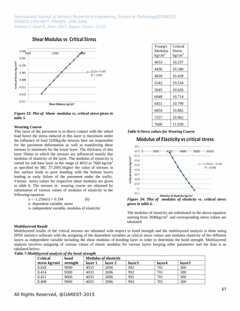
Figure 33: Plot of Shear modulus vs. critical stress given in

table 5.

Wearing Course

This layer of the pavement is in direct contact with the wheel

load hence the stress induced in this layer is maximum under

the influence of load 5100kg.the stresses here are responsible

for the pavement deformation as well as transferring these

stresses to minimum for the lower layer. The thickness of this

layer 50mm in which the stresses are influenced mainly due

modulus of elasticity of the layer. The modulus of elasticity is

varied for sub base layer in the range of 4033 to 7660 kg/cm2

as specified by IRC 37:2001.Higher the value of stresses in

this surface leads to poor bonding with the bottom layers

leading to early failure of the pavement under the traffic.

Various stress values for respective shear modulus are given

in table 6. The stresses in wearing course are obtained by

substitution of various values of modulus of elasticity in the

following equation:

y = -1.25ln(x) + 0.194 (6)



Table 6:Stress values for Wearing Course


given in table 6.




tabulated

Multilayered Result

Multilayered results of the critical stresses are tabulated with respect to bond strength and the multilayered analysis is done using

SPSS statistics software with the assigning of the dependent variables as critical stress values and modulus elasticity of the different

layers as independent variable including the shear modulus of bonding layer in order to determine the bond strength. Multilayered

analysis involves assigning of various values of elastic modulus for various layers keeping other parameters and the data is as

tabulated below:

Table 7:Multilayered analysis of the bond strength

Critical

stress kg/cm2

bond

strength

Modulus of elasticity

layer 1 layer 2 layer3 layer4 layer5

8.418 9000 4033 2696 992 701 300

8.414 9300 4033 2696 992 701 300

8.411 9600 4033 2696 992 701 300

8.408 9900 4033 2696 992 701 300

Young's

Modulus

kg/cm2

Critical

Stress

kg/cm2

4033 10.237

4436 10.340

4839 10.439

5242 10.534

5645 10.626

6048 10.714

6451 10.799

6854 10.882

7257 10.962

7660 11.039



68


8.405 10200 4033 2696 992 701 300

8.403 10500 4033 2696 992 701 300

8.400 10800 4033 2696 992 701 300

8.397 11100 4033 2696 992 701 300

8.394 11400 4033 2696 992 701 300

8.392 11700 4033 2696 992 701 300

10.237 11700 4033 2696 992 701 300

10.340 11700 4436 2696 992 701 300

10.439 11700 4839 2696 992 701 300

10.534 11700 5242 2696 992 701 300

10.626 11700 5645 2696 992 701 300

10.714 11700 6048 2696 992 701 300

10.799 11700 6451 2696 992 701 300

10.882 11700 6854 2696 992 701 300

10.962 11700 7257 2696 992 701 300

11.039 11700 7660 2696 992 701 300

7.450 11700 7660 2696 992 701 300

7.426 11700 7660 2916 992 701 300

7.402 11700 7660 3156 992 701 300

7.382 11700 7660 3386 992 701 300

7.350 11700 7660 3616 992 701 300

7.347 11700 7660 3846 992 701 300

7.332 11700 7660 4076 992 701 300

7.318 11700 7660 4306 992 701 300

7.306 11700 7660 4536 992 701 300

7.294 11700 7660 4766 992 701 300

8.392 11700 7660 4766 992 701 300

8.373 11700 7660 4766 1162 701 300

8.353 11700 7660 4766 1332 701 300

8.337 11700 7660 4766 1502 701 300

8.323 11700 7660 4766 1672 701 300

8.311 11700 7660 4766 1842 701 300

8.301 11700 7660 4766 2012 701 300

8.291 11700 7660 4766 2182 701 300

8.283 11700 7660 4766 2352 701 300

8.276 11700 7660 4766 2522 701 300

10.108 11700 7660 4766 2522 701 300

9.935 11700 7660 4766 2522 730 300

9.787 11700 7660 4766 2522 760 300

9.659 11700 7660 4766 2522 790 300

9.547 11700 7660 4766 2522 820 300

9.448 11700 7660 4766 2522 850 300

9.360 11700 7660 4766 2522 880 300

9.281 11700 7660 4766 2522 910 300

9.210 11700 7660 4766 2522 940 300

9.145 11700 7660 4766 2522 970 300

10.108 11700 7660 4766 2522 970 300

9.935 11700 7660 4766 2522 970 340

9.787 11700 7660 4766 2522 970 380

9.659 11700 7660 4766 2522 970 420

9.547 11700 7660 4766 2522 970 460

9.448 11700 7660 4766 2522 970 500

9.360 11700 7660 4766 2522 970 540



69


9.281 11700 7660 4766 2522 970 580

9.209 11700 7660 4766 2522 970 620

9.144 11700 7660 4766 2522 970 660

SPSS Statistics

Linear regression is the next step up after correlation. It is

used when we want to predict the value of a variable based on

the value of another variable. The variable we want to predict

is called the dependent variable (or sometimes, the outcome

variable). The variable we are using to predict the other

variable's value is called the independent variable (or

sometimes, the predictor variable).If you have two or more

independent variables, rather than just one, you need to

use multiple regression. In the present case the values of layers

are tabulated varying one particular property by keeping other

values constant. Procedure for multilayer Analysis:

1. Run the SPSS Statistics 17.0,a window appears as:

Figure 35: data sheet for entering the variables involved in

analysis.

2. Enter data of multilayer in various variable columns:

Figure 36:The data entered for multilayer regression

analysis

3. Go to the Analyze tab select regression as linear a tab pops

as shown below consisting of tabs for dependent and

independent variables. The stresses are assigned as

dependent variables and all other parameters as independent

variables and select ok as shown in figure 3:

Figure 37:Variable column 10 is assigned as independent

variable which is critical stress and other variable

columns as dependent variables.

4. The analysis consists of various tests such as ANOVA

Table, Model summary and coefficients table as output as

shown in figure 4:

Figure 36:Values of coefficients obtained for various

layers by method of F -test and T- test

Stress is computed as given by equation:

y = a1x1+ a2x2+ a3x3+ a4x4+ a5x5......

where y= Bond stress

a1 - Coefficient for sub-grade = 0.000

a2 - Coefficient for sub-base= 0.001

a3 - Coefficient for base=-0.001

a4 - Coefficient for binder course=-0.002

a5 - Coefficient for surface layer=0.001

Bond stress for a particular set of values is calculated as:

Stress =( 0.000 x Modulus of elasticity of sub grade +0.001 x

Modulus of elasticity of sub base - 0.001 x Modulus of

elasticity of base - 0.002 x Modulus of elasticity of binder

course + 0.001 x Modulus of elasticity of surface)



70


T test

The t-test looks at the t-statistic, t-distribution and degrees of

freedom to determine a p value (probability) that can be used

to determine whether the population means differ. The t-test is

one of a number of hypothesis tests. To compare three or more

variables, statisticians use an analysis of variance (ANOVA).

F Test

An F-test i.e. test of best fit is any statistical test in which the

test statistic has an F-distribution under the null hypothesis. It

is most often used when comparing statistical models that

have been fitted to a data set, in order to identify the model

that best fits the population from which the data were sampled.

14. Conclusions

Following conclusions could be drawn from this study:

1. The equation for stress in sub grade layer is given by the

equation: y=0.002x-10.80

2. The equation for stress in sub base layer is given by the

equation: y = 2.915ln(x) - 29.14

3. The equation for stress in base layer is given by the equation:

y = 7E-05x - 8.455

4. The equation for stress in binder course is given by the

equation: y = 7E-05x - 7.637

5. The equation for stress in bonding layer is given by the

equation: y = 1E-05x - 8.502

6. The equation for stress in surface layer is given by the

equation: y = -1.25ln(x) + 0.194

7. Bond strength is obtained by the following equation:

Y =( 0.000 x Modulus of elasticity of sub grade +0.001 x

Modulus of elasticity of sub base -0.001 x Modulus of

elasticity of base - 0.002 x Modulus of elasticity of binder

course + 0.001 x Modulus of elasticity of surface)

8. Better bonding condition at the interface between various

layers of the flexible pavement is ascertained by the

decreasing values of critical strain for wearing course, contact

layer, binder course, base layer and sub base. As the results,

the better structural capacity can be achieved with better

bonding between layers.

9. The performance of the pavement under given static wheel

load has deformed elastically inducing maximum and

minimum stresses. The minimum or critical stress values are

obtained from the equations generated.

10. The variation of the shear modulus has direct impact on

performance of the pavement.

11. The multilayer analysis of the pavement is analysed and the

bond stress is determined based on the equations.

References:

[1] Nagrale Prashant P, More Deepak (2014),Benefits Of

Mechanistic Approach In Flexible Pavement Design,

Indian Highways Vol.42 No.3.

[2] Xiaoyang Jia Baoshan Huang and Lihan (2013),

Evaluating Interlayer Shear Resistance In Asphalt

Pavement, Li-Tongji University Shanghai

[3] Xingsong Sun,(2011), Modelling Analysis Of Pavement

Layer Interface Bonding Condition Effects On Cracking

Performance, A Dissertation Presented To The Graduate

School Of The University Of Florida In Partial

Fulfillment Of The Requirements For The Degree Of

Doctor Of Philosophy, University Of Florida

[4] Bidyut Bikash Sutradhar(2010), Evaluation Of Bond

Between Bituminous Pavement Layers, A thesis submitted

in Partial fulfilment of the Master Of Technology In Civil

Engineering.

[5] Muslich Hartadi Sutanto, ST,MT, (2009),Assessment Of

Bond Between Asphalt Layers, PhD thesis, University of

Nottingham.

[6] Horak, E., Emery. S., Maina, J. W., Walker, B. (2009)

Mechanistic Modelling of Potential Interlayer Slip at Base

Sub-Base Level. 8th International Conference on the

BearingCapacity of Roads, Railways, and Airfields.

[7] Maurice Wheat (2007), Evaluation Of Bond Strength At

Asphalt Interfaces. A Report submitted in partial fulfilment

of the requirements for the degree Master Of Science

Department of Civil Engineering College of Engineering

KANSAS STATE UNIVERSITY, Manhattan, Kansas

[8] Laith Tashman(2006), Evaluation Of The Influence Of

Tack Coat Construction Factors On The Bond Strength

Between Pavement Layers, Report Prepared for

Washington State Department of Transportation.

[9] Hakim, B. A. (2002) The Importance of Good Bond

between Bituminous Layers. Proceedings of the 9th

International Conference on the Structural Design of

Asphalt Pavements.

[10] Hachiya, Y. and Sato, K. (1998) Effect of Tack Coat on

Bonding Characteristics at Interface between Asphalt

Concrete Layers. Proceedings of 8th International

Conference on Asphalt Pavements, Vol. 1. pp. 349-362.

[11]West, R., Moore, J., and Zhang, J. (2005). Evaluation of

Bond Strength Between Pavement Layers. NCAT Report

05-08, National Center for Asphalt Technology, Auburn,

Alabama

Effect of Bond Strength on Performance of Pavement

Documents

Transcript of Effect of Bond Strength on Performance of Pavement