Journal of Policy Modeling 31 (2009) 325–340

Available online at www.sciencedirect.com

Effect of agricultural policy on regional incomeinequality among farm households

Ashok Mishra a,∗, Hisham El-Osta b,1, Jeffrey M. Gillespie c,2

a 226 Ag. Admin. Bldg., Department of Agricultural Economics and Agribusiness,Louisiana State University AgCenter, Baton Rouge, LA 70803, United States

b Economic Research Service, U.S. Department of Agriculture,N4067, 1800 M St. NW, Washington, DC 20036-5831, United States

c 279 Ag. Admin. Bldg., Department of Agricultural Economics and Agribusiness,Louisiana State University AgCenter, Baton Rouge, LA 70803, United States

Received 1 July 2008; received in revised form 1 August 2008; accepted 1 December 2008Available online 7 February 2009

Abstract

Policymakers are under constant pressure to alleviate financial stress, mainly associated with farm businessincome, on farm households through government farm program payments. The 1996 FAIR Act signaled theend of these payments and Congress decided that agricultural policy should be more market oriented. Usingthe Gini coefficient concept and a large farm-level dataset, this study investigates the impact of governmentpayments on income inequality among farm households in nine farming resource regions of the U.S. Resultsindicate that distribution of income among farm households in the Fruitful Rim region was above the levelof dispersion for all U.S. farm households; however, income inequality in the Heartland region was belowthe level of dispersion for all U.S. farm households. Finally, income from government farm programs helpedreduce total income inequality in the Heartland and Northern Great Plains regions, while income from off-farm wages and/or salaries played an important role in reducing total income inequality in Basin and Rangeand Fruitful Rim regions of the U.S. farm sector.© 2009 Society for Policy Modeling. Published by Elsevier Inc. All rights reserved.

JEL classification: D31; Q12; Q18

Keywords: Income inequality; Off-farm income; Government farm program payments; Adjusted Gini coefficient; Farmresource regions

∗ Corresponding author. Tel.: +1 225 578 0262.E-mail addresses: amishra@lsu.edu (A. Mishra), Helsota@ers.usda.gov (H. El-Osta), jmgille@lsu.edu

(J.M. Gillespie).1 Tel.: +1 202 694 5564.2 Tel.: +1 225 578 2759.

0161-8938/$ – see front matter © 2009 Society for Policy Modeling. Published by Elsevier Inc. All rights reserved.doi:10.1016/j.jpolmod.2008.12.007

326 A. Mishra et al. / Journal of Policy Modeling 31 (2009) 325–340

Nearly seven decades ago, farm subsidies were promoted by concerns for the chronicallylow and highly variable incomes of U.S. farm households. A key stimulus for legislative actionwas disparity between incomes of farm and nonfarm households (Gardner, 1992; Houthakker,1967). In the 1990s, a major farm bill was passed, the 1996 Federal Agricultural Improve-ment and Reform (FAIR) Act, which greatly changed U.S. farm policies for its term andsubsequent farm bills. The FAIR Act allowed producers greater flexibility in cropping deci-sions, but also a fixed-but-decreasing production flexibility contract (transition) payment overthe next 7 years (Hoppe, 2001). The Act3 also provided nonrecourse marketing assistanceloans with marketing loan repayment (MLA) and loan deficiency payments (LDPs) for selectedcrops.

In 2002, the Farm Security and Rural Investment (FSRI) Act was signed into law and largelyextended the policies of the FAIR Act. While the marketing loan program and direct paymentscontinued, a new “countercyclical payment” was introduced. According to critics, the new farm billsuffered the same shortfall as the previous one: large farms continued to receive a disproportionateshare of payments. Martin (2002) adds that government payments, particularly since FAIR, haveallowed large farms to become even larger when payments were used for land purchase. This andthe argument that FSRI shifted support further toward landowners (via higher land values andlease rates) and away from farmers with no landholdings are apt to raise concerns on the impactof government payments on the distribution of farm household income.

The U.S. has witnessed increased economic growth over the last decade, with increased stockprices, consumer spending, and trade, yielding low unemployment and inflation as well as growingincome inequality. Mishra, El-Osta, Morehart, Johnson, and Hopkins (2002) find greater incomeinequality in farm compared to nonfarm households, as well as regional differences: incomeinequality is highest for farm households located in the South and Northeast regions and lowestin the North Central region.

A system of economically viable, midsized, owner-operated family farms contributes more tocommunities than systems characterized by inequality, larger numbers of farm laborers with belowaverage incomes, and little ownership or control of productive assets (Hassebrook, 1999). Farmincome inequality negatively impacts: (1) economic well-being, including farm family health;(2) farm technology adoption; (3) agricultural productivity; and (4) agricultural sector growth. Itis important to understand the role government farm program payments have played in incomeinequality among farm households. Regional differences are of interest.

The objectives of this paper are to determine: (1) the dimensions of income inequality amongfarm operator households, (2) the sources of income inequality, particularly the role of gov-ernment payments, (3) differences in farm household income inequality by region (Fig. 1),and (4) the contributions of sources of household income to inequality. We use a nationalfarm-level database with a larger, more representative sample than previous studies on thissubject.

1. Sources and trends in farm household income

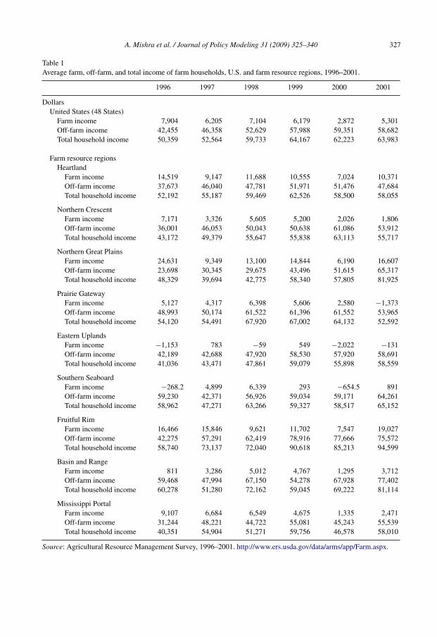
Total farm household income is defined as income from both the farming operation and off-farm sources. Table 1 shows the composition of farm household income. For majority of U.S.

3 Under FAIR, a farm was eligible for production flexibility contract payments if it had at least one crop acreage basein a production adjustment program for any of the crop years 1991 through 1995.

A. Mishra et al. / Journal of Policy Modeling 31 (2009) 325–340 327

Table 1Average farm, off-farm, and total income of farm households, U.S. and farm resource regions, 1996–2001.

1996 1997 1998 1999 2000 2001

DollarsUnited States (48 States)

Farm income 7,904 6,205 7,104 6,179 2,872 5,301Off-farm income 42,455 46,358 52,629 57,988 59,351 58,682Total household income 50,359 52,564 59,733 64,167 62,223 63,983

Farm resource regionsHeartland

Farm income 14,519 9,147 11,688 10,555 7,024 10,371Off-farm income 37,673 46,040 47,781 51,971 51,476 47,684Total household income 52,192 55,187 59,469 62,526 58,500 58,055

Northern CrescentFarm income 7,171 3,326 5,605 5,200 2,026 1,806Off-farm income 36,001 46,053 50,043 50,638 61,086 53,912Total household income 43,172 49,379 55,647 55,838 63,113 55,717

Northern Great PlainsFarm income 24,631 9,349 13,100 14,844 6,190 16,607Off-farm income 23,698 30,345 29,675 43,496 51,615 65,317Total household income 48,329 39,694 42,775 58,340 57,805 81,925

Prairie GatewayFarm income 5,127 4,317 6,398 5,606 2,580 −1,373Off-farm income 48,993 50,174 61,522 61,396 61,552 53,965Total household income 54,120 54,491 67,920 67,002 64,132 52,592

Eastern UplandsFarm income −1,153 783 −59 549 −2,022 −131Off-farm income 42,189 42,688 47,920 58,530 57,920 58,691Total household income 41,036 43,471 47,861 59,079 55,898 58,559

Southern SeaboardFarm income −268.2 4,899 6,339 293 −654.5 891Off-farm income 59,230 42,371 56,926 59,034 59,171 64,261Total household income 58,962 47,271 63,266 59,327 58,517 65,152

Fruitful RimFarm income 16,466 15,846 9,621 11,702 7,547 19,027Off-farm income 42,275 57,291 62,419 78,916 77,666 75,572Total household income 58,740 73,137 72,040 90,618 85,213 94,599

Basin and RangeFarm income 811 3,286 5,012 4,767 1,295 3,712Off-farm income 59,468 47,994 67,150 54,278 67,928 77,402Total household income 60,278 51,280 72,162 59,045 69,222 81,114

Mississippi PortalFarm income 9,107 6,684 6,549 4,675 1,335 2,471Off-farm income 31,244 48,221 44,722 55,081 45,243 55,539Total household income 40,351 54,904 51,271 59,756 46,578 58,010

Source: Agricultural Resource Management Survey, 1996–2001. http://www.ers.usda.gov/data/arms/app/Farm.aspx.

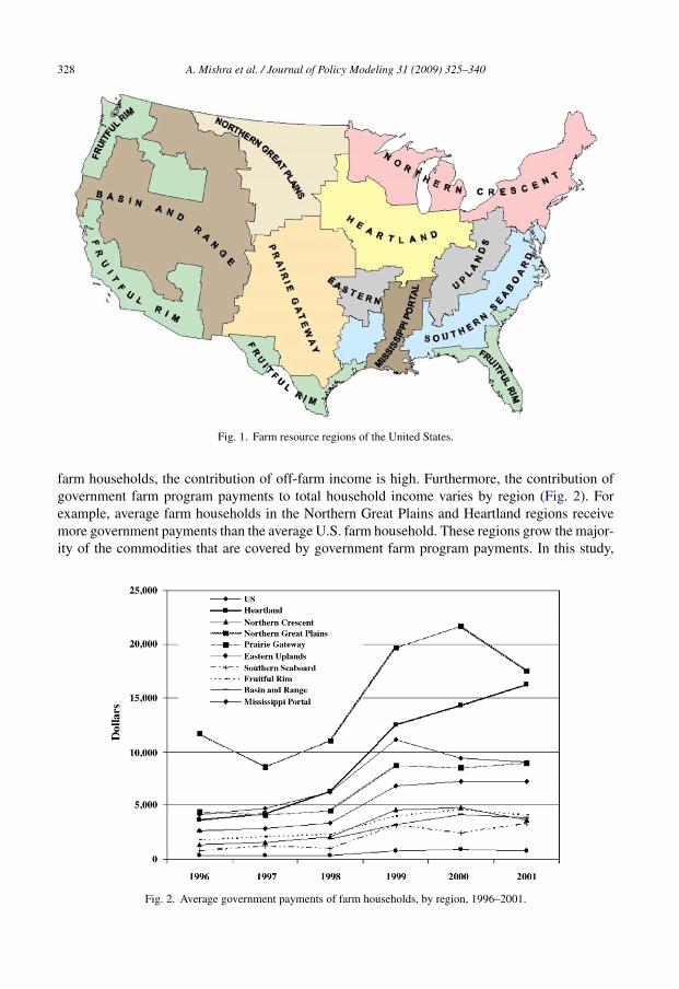
328 A. Mishra et al. / Journal of Policy Modeling 31 (2009) 325–340

Fig. 1. Farm resource regions of the United States.

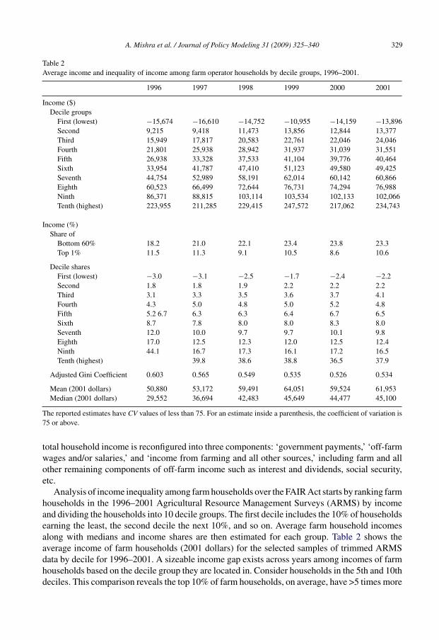
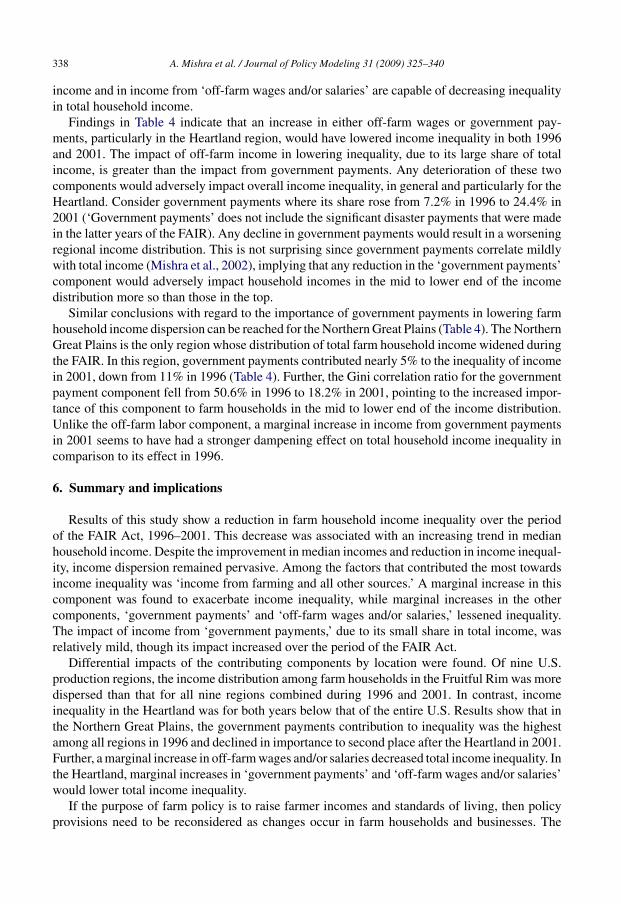
farm households, the contribution of off-farm income is high. Furthermore, the contribution ofgovernment farm program payments to total household income varies by region (Fig. 2). Forexample, average farm households in the Northern Great Plains and Heartland regions receivemore government payments than the average U.S. farm household. These regions grow the major-ity of the commodities that are covered by government farm program payments. In this study,

Fig. 2. Average government payments of farm households, by region, 1996–2001.

A. Mishra et al. / Journal of Policy Modeling 31 (2009) 325–340 329

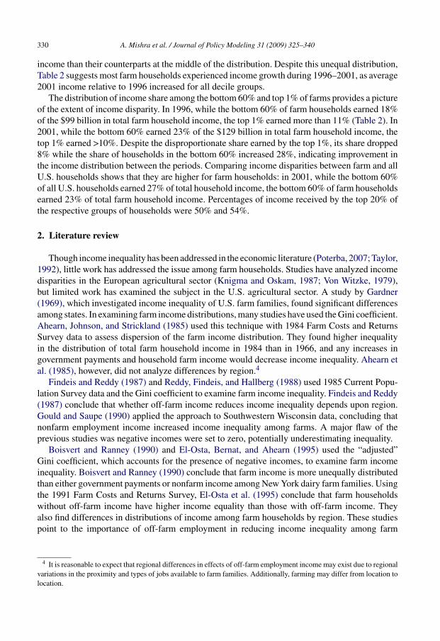
Table 2Average income and inequality of income among farm operator households by decile groups, 1996–2001.

1996 1997 1998 1999 2000 2001

Income ($)Decile groups

First (lowest) −15,674 −16,610 −14,752 −10,955 −14,159 −13,896Second 9,215 9,418 11,473 13,856 12,844 13,377Third 15,949 17,817 20,583 22,761 22,046 24,046Fourth 21,801 25,938 28,942 31,937 31,039 31,551Fifth 26,938 33,328 37,533 41,104 39,776 40,464Sixth 33,954 41,787 47,410 51,123 49,580 49,425Seventh 44,754 52,989 58,191 62,014 60,142 60,866Eighth 60,523 66,499 72,644 76,731 74,294 76,988Ninth 86,371 88,815 103,114 103,534 102,133 102,066Tenth (highest) 223,955 211,285 229,415 247,572 217,062 234,743

Income (%)Share of

Bottom 60% 18.2 21.0 22.1 23.4 23.8 23.3Top 1% 11.5 11.3 9.1 10.5 8.6 10.6

Decile sharesFirst (lowest) −3.0 −3.1 −2.5 −1.7 −2.4 −2.2Second 1.8 1.8 1.9 2.2 2.2 2.2Third 3.1 3.3 3.5 3.6 3.7 4.1Fourth 4.3 5.0 4.8 5.0 5.2 4.8Fifth 5.2 6.7 6.3 6.3 6.4 6.7 6.5Sixth 8.7 7.8 8.0 8.0 8.3 8.0Seventh 12.0 10.0 9.7 9.7 10.1 9.8Eighth 17.0 12.5 12.3 12.0 12.5 12.4Ninth 44.1 16.7 17.3 16.1 17.2 16.5Tenth (highest) 39.8 38.6 38.8 36.5 37.9

Adjusted Gini Coefficient 0.603 0.565 0.549 0.535 0.526 0.534

Mean (2001 dollars) 50,880 53,172 59,491 64,051 59,524 61,953Median (2001 dollars) 29,552 36,694 42,483 45,649 44,477 45,100

The reported estimates have CV values of less than 75. For an estimate inside a parenthesis, the coefficient of variation is75 or above.

total household income is reconfigured into three components: ‘government payments,’ ‘off-farmwages and/or salaries,’ and ‘income from farming and all other sources,’ including farm and allother remaining components of off-farm income such as interest and dividends, social security,etc.

Analysis of income inequality among farm households over the FAIR Act starts by ranking farmhouseholds in the 1996–2001 Agricultural Resource Management Surveys (ARMS) by incomeand dividing the households into 10 decile groups. The first decile includes the 10% of householdsearning the least, the second decile the next 10%, and so on. Average farm household incomesalong with medians and income shares are then estimated for each group. Table 2 shows theaverage income of farm households (2001 dollars) for the selected samples of trimmed ARMSdata by decile for 1996–2001. A sizeable income gap exists across years among incomes of farmhouseholds based on the decile group they are located in. Consider households in the 5th and 10thdeciles. This comparison reveals the top 10% of farm households, on average, have >5 times more

330 A. Mishra et al. / Journal of Policy Modeling 31 (2009) 325–340

income than their counterparts at the middle of the distribution. Despite this unequal distribution,Table 2 suggests most farm households experienced income growth during 1996–2001, as average2001 income relative to 1996 increased for all decile groups.

The distribution of income share among the bottom 60% and top 1% of farms provides a pictureof the extent of income disparity. In 1996, while the bottom 60% of farm households earned 18%of the $99 billion in total farm household income, the top 1% earned more than 11% (Table 2). In2001, while the bottom 60% earned 23% of the $129 billion in total farm household income, thetop 1% earned >10%. Despite the disproportionate share earned by the top 1%, its share dropped8% while the share of households in the bottom 60% increased 28%, indicating improvement inthe income distribution between the periods. Comparing income disparities between farm and allU.S. households shows that they are higher for farm households: in 2001, while the bottom 60%of all U.S. households earned 27% of total household income, the bottom 60% of farm householdsearned 23% of total farm household income. Percentages of income received by the top 20% ofthe respective groups of households were 50% and 54%.

2. Literature review

Though income inequality has been addressed in the economic literature (Poterba, 2007; Taylor,1992), little work has addressed the issue among farm households. Studies have analyzed incomedisparities in the European agricultural sector (Knigma and Oskam, 1987; Von Witzke, 1979),but limited work has examined the subject in the U.S. agricultural sector. A study by Gardner(1969), which investigated income inequality of U.S. farm families, found significant differencesamong states. In examining farm income distributions, many studies have used the Gini coefficient.Ahearn, Johnson, and Strickland (1985) used this technique with 1984 Farm Costs and ReturnsSurvey data to assess dispersion of the farm income distribution. They found higher inequalityin the distribution of total farm household income in 1984 than in 1966, and any increases ingovernment payments and household farm income would decrease income inequality. Ahearn etal. (1985), however, did not analyze differences by region.4

Findeis and Reddy (1987) and Reddy, Findeis, and Hallberg (1988) used 1985 Current Popu-lation Survey data and the Gini coefficient to examine farm income inequality. Findeis and Reddy(1987) conclude that whether off-farm income reduces income inequality depends upon region.Gould and Saupe (1990) applied the approach to Southwestern Wisconsin data, concluding thatnonfarm employment income increased income inequality among farms. A major flaw of theprevious studies was negative incomes were set to zero, potentially underestimating inequality.

Boisvert and Ranney (1990) and El-Osta, Bernat, and Ahearn (1995) used the “adjusted”Gini coefficient, which accounts for the presence of negative incomes, to examine farm incomeinequality. Boisvert and Ranney (1990) conclude that farm income is more unequally distributedthan either government payments or nonfarm income among New York dairy farm families. Usingthe 1991 Farm Costs and Returns Survey, El-Osta et al. (1995) conclude that farm householdswithout off-farm income have higher income equality than those with off-farm income. Theyalso find differences in distributions of income among farm households by region. These studiespoint to the importance of off-farm employment in reducing income inequality among farm

4 It is reasonable to expect that regional differences in effects of off-farm employment income may exist due to regionalvariations in the proximity and types of jobs available to farm families. Additionally, farming may differ from location tolocation.

A. Mishra et al. / Journal of Policy Modeling 31 (2009) 325–340 331

families, hence the importance of rural development policies aimed at promoting better off-farmwork opportunities. Using 1997 ARMS data and the adjusted Gini coefficient, Mishra et al. (2002)found that the distribution of farm income was more unequal than that of wealth and farm locationplayed a role in income inequality. Mishra et al. (2002) had several weaknesses. They used only1 year of data to examine income inequality, aggregated the data into only four regions, and didnot investigate sources of income inequality.

This paper extends previous research on farm income inequality by using a method thatimproves the accuracy of Gini coefficient estimates. Data are grouped into nine farm resourceregions that merge information about land characteristics and commodities produced, cut acrossstate boundaries, and are more homogenous with regard to resource and production activi-ties. Unlike Boisvert and Ranney, we examine regional income inequality and consider moneyand non-money income, as suggested by Larson and Carlin (1974). Unlike Ahearn et al., weexclude the 3% of farms organized as non-family corporations, cooperatives, or managed byoperators not sharing in the net income of the business. In contrast to the Current Popula-tion Survey used by Findeis and Reddy (1987) and Reddy et al. (1988), the ARMS dataincludes farm households residing both on and off the farm. About 20% of all U.S. farmhouseholds reside off their farms (Mishra et al., 2002). Ahearn et al. (1985) report that thesefarm households earn more money from government programs and off-farm work than thosethat reside on the farm. Finally, we include farm-level data for 6 years (1996–2001). Sincemost farm households have steady sources of off-farm income from wages and salaried jobs(Mishra et al., 2002), this study includes income from wages and salaried jobs as off-farmincome.

3. Measurement of inequality

In cases where the income of each household is non-negative, the standard Gini coefficient(referred to as just the Gini coefficient) with range [0,1] provides a relative measure of inequality.5

If farm household income, for example, is equally distributed, the Gini coefficient would be 0.With greater income inequality, the Gini coefficient approaches a value of 1. Where income iscomprised of k components, the Gini coefficient for the kth income component, Yk, is definedbased on Pyatt, Chen, and Fei (1980) and extended by Lerman and Yitzhaki (1985) as:

G(Yk) = 2 cov[Yk, F (Yk)]

Yk

, (1)

where F(Yk) is the cumulative distribution of Yk (ranked in nondecreasing order), Yk is the meanof Yk, and cov is a covariance indicator.

Let n denote the sample size. The estimator of F(Yk) in a random sample is the rank of Ykdivided by n. In a weighted sample where wi is the survey weight that corresponds to the ithhousehold,

∑ni=1wi = 1, w0 = 0, and the estimator of F(Yk) is a mid-interval of F(Yk) or

Fi(Yk) =i−1∑j=0

wj + wi

2(2)

5 This measure of inequality dates back to 1912 when it was formulated by the Italian statistician Corrado Gini.

332 A. Mishra et al. / Journal of Policy Modeling 31 (2009) 325–340

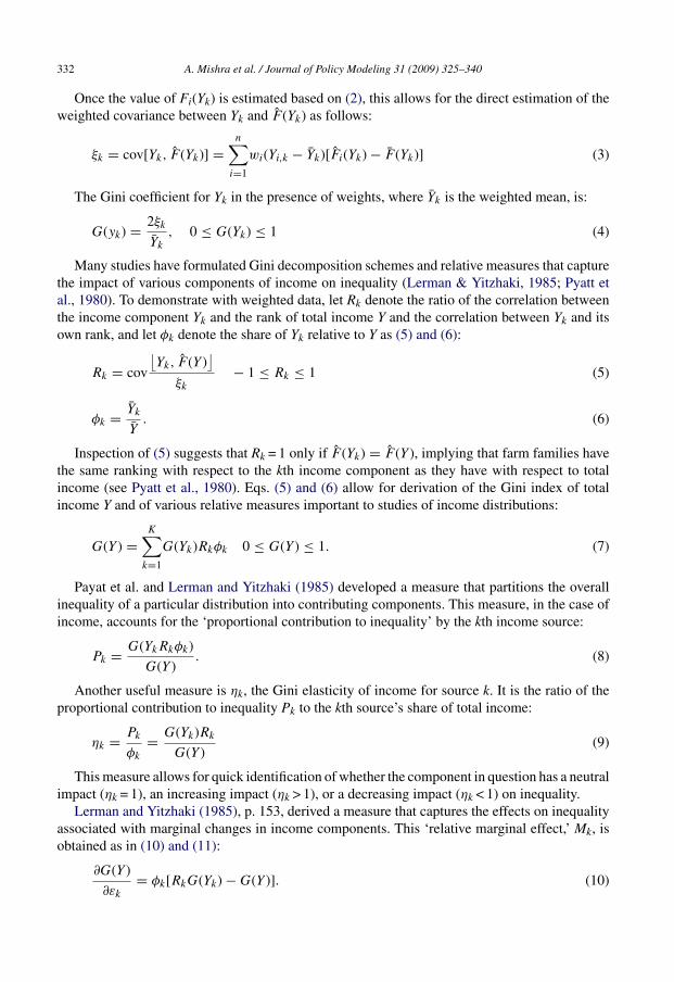
Once the value of Fi(Yk) is estimated based on (2), this allows for the direct estimation of theweighted covariance between Yk and F (Yk) as follows:

ξk = cov[Yk, F (Yk)] =n∑

i=1

wi(Yi,k − Yk)[Fi(Yk) − F (Yk)] (3)

The Gini coefficient for Yk in the presence of weights, where Yk is the weighted mean, is:

G(yk) = 2ξk

Yk

, 0 ≤ G(Yk) ≤ 1 (4)

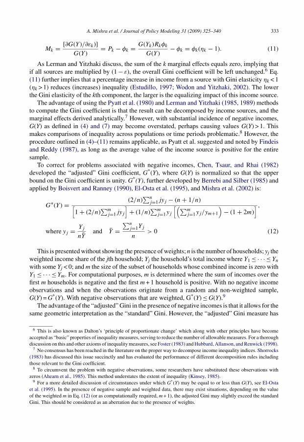
Many studies have formulated Gini decomposition schemes and relative measures that capturethe impact of various components of income on inequality (Lerman & Yitzhaki, 1985; Pyatt etal., 1980). To demonstrate with weighted data, let Rk denote the ratio of the correlation betweenthe income component Yk and the rank of total income Y and the correlation between Yk and itsown rank, and let φk denote the share of Yk relative to Y as (5) and (6):

Rk = cov

⌊Yk, F (Y )

⌋

ξk

− 1 ≤ Rk ≤ 1 (5)

φk = Yk

Y. (6)

Inspection of (5) suggests that Rk = 1 only if F (Yk) = F (Y ), implying that farm families havethe same ranking with respect to the kth income component as they have with respect to totalincome (see Pyatt et al., 1980). Eqs. (5) and (6) allow for derivation of the Gini index of totalincome Y and of various relative measures important to studies of income distributions:

G(Y ) =K∑

k=1

G(Yk)Rkφk 0 ≤ G(Y ) ≤ 1. (7)

Payat et al. and Lerman and Yitzhaki (1985) developed a measure that partitions the overallinequality of a particular distribution into contributing components. This measure, in the case ofincome, accounts for the ‘proportional contribution to inequality’ by the kth income source:

Pk = G(YkRkφk)

G(Y ). (8)

Another useful measure is ηk, the Gini elasticity of income for source k. It is the ratio of theproportional contribution to inequality Pk to the kth source’s share of total income:

ηk = Pk

φk

= G(Yk)Rk

G(Y )(9)

This measure allows for quick identification of whether the component in question has a neutralimpact (ηk = 1), an increasing impact (ηk > 1), or a decreasing impact (ηk < 1) on inequality.

Lerman and Yitzhaki (1985), p. 153, derived a measure that captures the effects on inequalityassociated with marginal changes in income components. This ‘relative marginal effect,’ Mk, isobtained as in (10) and (11):

∂G(Y )

∂εk

= φk[RkG(Yk) − G(Y )]. (10)

A. Mishra et al. / Journal of Policy Modeling 31 (2009) 325–340 333

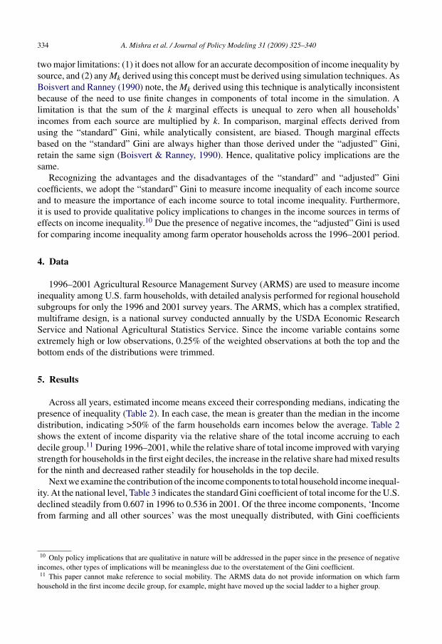
Mk = [∂G(Y )/∂εk)]

G(Y )= Pk − φk = G(Yk)Rkφk

G(Y )− φk = φk(ηk − 1). (11)

As Lerman and Yitzhaki discuss, the sum of the k marginal effects equals zero, implying thatif all sources are multiplied by (1 − ε), the overall Gini coefficient will be left unchanged.6 Eq.(11) further implies that a percentage increase in income from a source with Gini elasticity ηk < 1(ηk > 1) reduces (increases) inequality (Estudillo, 1997; Wodon and Yitzhaki, 2002). The lowerthe Gini elasticity of the kth component, the larger is the equalizing impact of this income source.

The advantage of using the Pyatt et al. (1980) and Lerman and Yitzhaki (1985, 1989) methodsto compute the Gini coefficient is that the result can be decomposed by income sources, and themarginal effects derived analytically.7 However, with substantial incidence of negative incomes,G(Y) as defined in (4) and (7) may become overstated, perhaps causing values G(Y) > 1. Thismakes comparisons of inequality across populations or time periods problematic.8 However, theprocedure outlined in (4)–(11) remains applicable, as Pyatt et al. suggested and noted by Findeisand Reddy (1987), as long as the average value of the income source is positive for the entiresample.

To correct for problems associated with negative incomes, Chen, Tsaur, and Rhai (1982)developed the “adjusted” Gini coefficient, G*(Y), where G(Y) is normalized so that the upperbound on the Gini coefficient is unity. G*(Y), further developed by Berrebi and Silber (1985) andapplied by Boisvert and Ranney (1990), El-Osta et al. (1995), and Mishra et al. (2002) is:

G∗(Y ) = (2/n)∑n

j=1jyj − (n + 1/n)[1 + (2/n)

∑mj=1jyj

]+ (1/n)

∑mj=1yj

[(∑mj=1yj/ym+1

)− (1 + 2m)

] ,

where yj = Yj

nYand Y =

∑nj=1Yj

n> 0 (12)

This is presented without showing the presence of weights; n is the number of households; yj theweighted income share of the jth household; Yj the household’s total income where Y1 ≤ · · · ≤ Yn

with some Yj < 0; and m the size of the subset of households whose combined income is zero withY1 ≤ · · · ≤ Ym. For computational purposes, m is determined where the sum of incomes over thefirst m households is negative and the first m + 1 household is positive. With no negative incomeobservations and when the observations originate from a random and non-weighted sample,G(Y) = G*(Y). With negative observations that are weighted, G*(Y) ≤ G(Y).9

The advantage of the “adjusted” Gini in the presence of negative incomes is that it allows for thesame geometric interpretation as the “standard” Gini. However, the “adjusted” Gini measure has

6 This is also known as Dalton’s ‘principle of proportionate change’ which along with other principles have becomeaccepted as “basic” properties of inequality measures, serving to reduce the number of allowable measures. For a thoroughdiscussion on this and other axioms of inequality measures, see Foster (1983) and Hubbard, Allanson, and Renwick (1998).

7 No consensus has been reached in the literature on the proper way to decompose income inequality indices. Shorrocks(1983) has discussed this issue succinctly and has evaluated the performance of different decomposition rules includingthose relevant to the Gini coefficient.

8 To circumvent the problem with negative observations, some researchers have substituted these observations withzeros (Ahearn et al., 1985). This method understates the extent of inequality (Kinsey, 1985).

9 For a more detailed discussion of circumstances under which G*(Y) may be equal to or less than G(Y), see El-Ostaet al. (1995). In the presence of negative sample and weighted data, there may exist situations, depending on the valueof the weighted m in Eq. (12) (or as computationally required, m + 1), the adjusted Gini may slightly exceed the standardGini. This should be considered as an aberration due to the presence of weights.

334 A. Mishra et al. / Journal of Policy Modeling 31 (2009) 325–340

two major limitations: (1) it does not allow for an accurate decomposition of income inequality bysource, and (2) any Mk derived using this concept must be derived using simulation techniques. AsBoisvert and Ranney (1990) note, the Mk derived using this technique is analytically inconsistentbecause of the need to use finite changes in components of total income in the simulation. Alimitation is that the sum of the k marginal effects is unequal to zero when all households’incomes from each source are multiplied by k. In comparison, marginal effects derived fromusing the “standard” Gini, while analytically consistent, are biased. Though marginal effectsbased on the “standard” Gini are always higher than those derived under the “adjusted” Gini,retain the same sign (Boisvert & Ranney, 1990). Hence, qualitative policy implications are thesame.

Recognizing the advantages and the disadvantages of the “standard” and “adjusted” Ginicoefficients, we adopt the “standard” Gini to measure income inequality of each income sourceand to measure the importance of each income source to total income inequality. Furthermore,it is used to provide qualitative policy implications to changes in the income sources in terms ofeffects on income inequality.10 Due the presence of negative incomes, the “adjusted” Gini is usedfor comparing income inequality among farm operator households across the 1996–2001 period.

4. Data

1996–2001 Agricultural Resource Management Survey (ARMS) are used to measure incomeinequality among U.S. farm households, with detailed analysis performed for regional householdsubgroups for only the 1996 and 2001 survey years. The ARMS, which has a complex stratified,multiframe design, is a national survey conducted annually by the USDA Economic ResearchService and National Agricultural Statistics Service. Since the income variable contains someextremely high or low observations, 0.25% of the weighted observations at both the top and thebottom ends of the distributions were trimmed.

5. Results

Across all years, estimated income means exceed their corresponding medians, indicating thepresence of inequality (Table 2). In each case, the mean is greater than the median in the incomedistribution, indicating >50% of the farm households earn incomes below the average. Table 2shows the extent of income disparity via the relative share of the total income accruing to eachdecile group.11 During 1996–2001, while the relative share of total income improved with varyingstrength for households in the first eight deciles, the increase in the relative share had mixed resultsfor the ninth and decreased rather steadily for households in the top decile.

Next we examine the contribution of the income components to total household income inequal-ity. At the national level, Table 3 indicates the standard Gini coefficient of total income for the U.S.declined steadily from 0.607 in 1996 to 0.536 in 2001. Of the three income components, ‘Incomefrom farming and all other sources’ was the most unequally distributed, with Gini coefficients

10 Only policy implications that are qualitative in nature will be addressed in the paper since in the presence of negativeincomes, other types of implications will be meaningless due to the overstatement of the Gini coefficient.11 This paper cannot make reference to social mobility. The ARMS data do not provide information on which farm

household in the first income decile group, for example, might have moved up the social ladder to a higher group.

A. Mishra et al. / Journal of Policy Modeling 31 (2009) 325–340 335

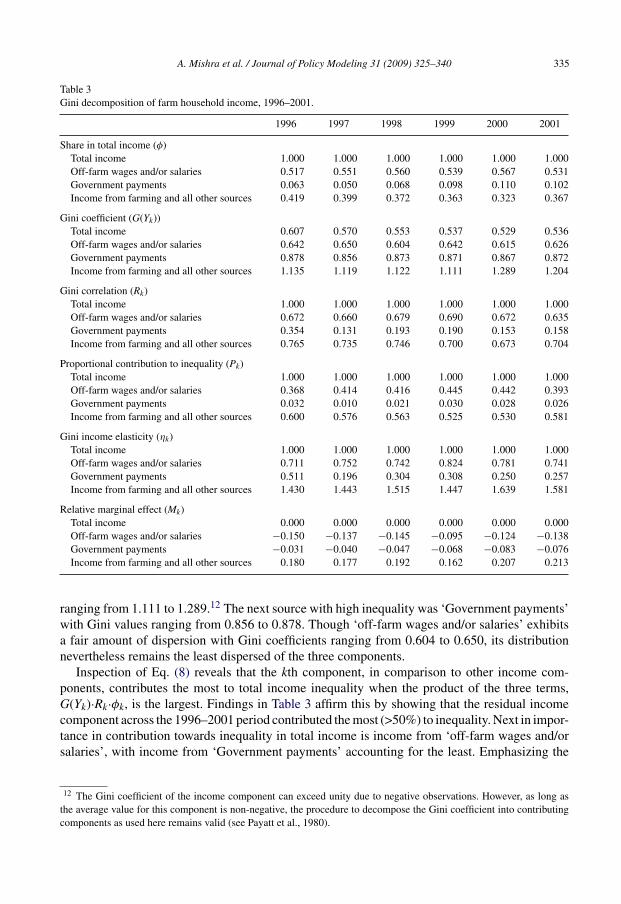
Table 3Gini decomposition of farm household income, 1996–2001.

1996 1997 1998 1999 2000 2001

Share in total income (φ)Total income 1.000 1.000 1.000 1.000 1.000 1.000Off-farm wages and/or salaries 0.517 0.551 0.560 0.539 0.567 0.531Government payments 0.063 0.050 0.068 0.098 0.110 0.102Income from farming and all other sources 0.419 0.399 0.372 0.363 0.323 0.367

Gini coefficient (G(Yk))Total income 0.607 0.570 0.553 0.537 0.529 0.536Off-farm wages and/or salaries 0.642 0.650 0.604 0.642 0.615 0.626Government payments 0.878 0.856 0.873 0.871 0.867 0.872Income from farming and all other sources 1.135 1.119 1.122 1.111 1.289 1.204

Gini correlation (Rk)Total income 1.000 1.000 1.000 1.000 1.000 1.000Off-farm wages and/or salaries 0.672 0.660 0.679 0.690 0.672 0.635Government payments 0.354 0.131 0.193 0.190 0.153 0.158Income from farming and all other sources 0.765 0.735 0.746 0.700 0.673 0.704

Proportional contribution to inequality (Pk)Total income 1.000 1.000 1.000 1.000 1.000 1.000Off-farm wages and/or salaries 0.368 0.414 0.416 0.445 0.442 0.393Government payments 0.032 0.010 0.021 0.030 0.028 0.026Income from farming and all other sources 0.600 0.576 0.563 0.525 0.530 0.581

Gini income elasticity (ηk)Total income 1.000 1.000 1.000 1.000 1.000 1.000Off-farm wages and/or salaries 0.711 0.752 0.742 0.824 0.781 0.741Government payments 0.511 0.196 0.304 0.308 0.250 0.257Income from farming and all other sources 1.430 1.443 1.515 1.447 1.639 1.581

Relative marginal effect (Mk)Total income 0.000 0.000 0.000 0.000 0.000 0.000Off-farm wages and/or salaries −0.150 −0.137 −0.145 −0.095 −0.124 −0.138Government payments −0.031 −0.040 −0.047 −0.068 −0.083 −0.076Income from farming and all other sources 0.180 0.177 0.192 0.162 0.207 0.213

ranging from 1.111 to 1.289.12 The next source with high inequality was ‘Government payments’with Gini values ranging from 0.856 to 0.878. Though ‘off-farm wages and/or salaries’ exhibitsa fair amount of dispersion with Gini coefficients ranging from 0.604 to 0.650, its distributionnevertheless remains the least dispersed of the three components.

Inspection of Eq. (8) reveals that the kth component, in comparison to other income com-ponents, contributes the most to total income inequality when the product of the three terms,G(Yk)·Rk·φk, is the largest. Findings in Table 3 affirm this by showing that the residual incomecomponent across the 1996–2001 period contributed the most (>50%) to inequality. Next in impor-tance in contribution towards inequality in total income is income from ‘off-farm wages and/orsalaries’, with income from ‘Government payments’ accounting for the least. Emphasizing the

12 The Gini coefficient of the income component can exceed unity due to negative observations. However, as long asthe average value for this component is non-negative, the procedure to decompose the Gini coefficient into contributingcomponents as used here remains valid (see Payatt et al., 1980).

336 A. Mishra et al. / Journal of Policy Modeling 31 (2009) 325–340

impact of these three income sources on inequality for 1996 and 2001 reveals that the contributionof residual income declined from 60.0% to 58.1%, respectively; that of off-farm labor incomeincreased from 36.8% to 39.3%; and that of government payments declined from 3.2% to 2.6%.

Table 3 also provides findings with regard to the Gini income elasticities (fifth panel) forthe three income components ηk. The Gini elasticity for residual income across the 1996–2001period are all >1, which, as noted earlier (see discussion of Eq. (11)), indicate that this incomesource is inequality increasing. The fact that the values of these elasticities are >1 indicates thata change in this income source affects the incomes of higher income farm households more, inpercentage terms, than it affects the incomes of lower income households, thereby increasinginequality. In comparison, both incomes from ‘Off-farm wages and/or salaries’ and ‘Governmentpayments’ have Gini elasticities with values <1, which suggests these factor components areinequality decreasing. Such interpretation implies that changes in these factors would impactthe farm households in the lower end of the income distribution more than they would impactthose at the top of the distribution. In terms of trends in ηk over the 1996–2001 period, results inTable 3 indicate a general rise in the unequilizing effect from residual income, a general drop inthe equalizing effect from off-farm wages and/or salaries, and a general increase in the equalizingeffect from government payments. Similar trends are observed from the results of the relativemarginal effects (Mk) of these components, as evident in the lower panel of Table 3.

Results in Table 4 show variation in income inequality based on the regional delineation of thedata. Three regions in 1996 (Southern Seaboard, Fruitful Rim, Basin and Range) and two in 2001(Northern Great Plains, Fruitful Rim) have income dispersion levels exceeding their correspondinglevels (i.e., 0.607 in 1996 and 0.536 in 2001) for the whole U.S. If income dispersion for a regionis higher than dispersion for the full sample, this suggests a potential means to lowering inequalityin the nationwide income distribution.13 In these five regions in 1996 and 2001 where incomedispersion exceeded the corresponding levels for the whole U.S., a question arises: which incomecomponents could be utilized to reduce total income inequality? Columns 2 and 6 in Table 4show the 1996 and 2001 proportional contribution to inequality by income source and region,respectively. For the Southern Seaboard and Fruitful Rim in 2001, because the ‘Income fromfarming and all other sources’ component in each of these regions contributes (i.e., Pk = 0.640and 0.627, respectively) measurably a larger share to inequality than it contributes to total incomein terms of relative share (i.e., φk = 0.450 and 0.393, respectively), marginal increases in thisincome component act to exacerbate income inequality rather than to reduce it (Table 4). Instead,income from off-farm wages and/or salaries in both of these regions in 1996, while it contributesa sizeable share towards inequality (i.e., Pk = 0.354 and 0.299, respectively, Table 4), this levelof contribution across 1996 remains lower than what it contributes (i.e., φk = 0.531 and 0.504,respectively) to the total household. This suggests a marginal increase in this component willdecrease inequality in total household income. Income from government payments in the SouthernSeaboard and Fruitful Rim, while accounting respectively for 2% and 10% of the total incomein 1996, contributed minimally to inequality in 1996 (0.6% and 7.4%). To the extent that thecontribution of government payments to inequality was less than its contribution to total income,a marginal increase in this income source in both of these regions is shown to decrease inequality,although minimally. In 2001, while only a marginal increase in income from government paymentsallows for a decrease in inequality in the Basin and Range, marginal increases in both this source of

13 Usage of phrases ‘full sample’, ‘nationwide’, ‘whole U.S.’, or ‘entire U.S.’ refers to farm-level data from the ARMSthat encompass only the 48-continguous states in the U.S.

A. Mishra et al. / Journal of Policy Modeling 31 (2009) 325–340 337

Table 4Gini decomposition of farm household income by farm resource regions, 1996 and 2001.

1996 2001

G(Yk) Pk ηk Mk G(Yk) Pk ηk Mk

HeartlandTotal income 0.541 1.000 1.000 0.000 0.488 1.000 1.000 0.000Off-farm wages and/or salaries 0.633 0.312 0.695 −0.137 0.579 0.287 0.565 −0.221Government payments 0.721 0.025 0.344 −0.047 0.707 0.062 0.254 −0.182Income from farming and all other sources 0.948 0.663 1.385 0.184 1.819 0.651 2.632 0.403

Northern CrescentTotal income 0.601 1.000 1.000 0.000 0.532 1.000 1.000 0.000Off-farm wages and/or salaries 0.665 0.390 0.737 −0.139 0.616 0.419 0.741 −0.146Government payments 0.837 0.003 0.112 −0.026 0.832 0.005 0.077 −0.055Income from farming and all other sources 1.095 0.607 1.375 0.165 1.207 0.576 1.536 0.201

Northern Great PlainsTotal income 0.605 1.000 1.000 0.000 0.613 1.000 1.000 0.000Off-farm wages and/or salaries 0.689 0.118 0.479 −0.128 0.776 0.491 1.013 0.007Government payments 0.618 0.114 0.516 −0.107 0.737 0.049 0.219 −0.176Income from farming and all other sources 0.977 0.768 1.440 0.235 1.344 0.460 1.584 0.170

Prairie GatewayTotal income 0.592 1.000 1.000 0.000 0.530 1.000 1.000 0.000Off-farm wages and/or salaries 0.594 0.345 0.673 −0.168 0.630 0.435 0.769 −0.131Government payments 0.805 0.025 0.308 −0.056 0.850 0.031 0.207 −0.118Income from farming and all other sources 1.140 0.630 1.549 0.223 1.568 0.534 1.871 0.249

Eastern UplandsTotal income 0.557 1.000 1.000 0.000 0.535 1.000 1.000 0.000Off-farm wages and/or salaries 0.611 0.602 0.885 −0.079 0.590 0.387 0.720 −0.151Government payments 0.947 0.001 0.146 −0.007 0.944 0.001 0.132 −0.010Income from farming and all other sources 1.153 0.397 1.277 0.086 0.981 0.611 1.356 0.161

Southern SeaboardTotal income 0.611 1.000 1.000 0.000 0.478 1.000 1.000 0.000Off-farm wages and/or salaries 0.623 0.354 0.667 −0.177 0.577 0.349 0.691 −0.157Government payments 0.942 0.006 0.319 −0.013 0.950 0.018 0.447 −0.022Income from farming and all other sources 1.122 0.640 1.421 0.190 0.910 0.633 1.392 0.178

Fruitful RimTotal income 0.772 1.000 1.000 0.000 0.609 1.000 1.000 0.000Off-farm wages and/or salaries 0.686 0.299 0.593 −0.205 0.655 0.382 0.723 −0.146Government payments 0.965 0.074 0.717 −0.029 0.958 0.016 0.432 −0.022Income from farming and all other sources 1.660 0.627 1.597 0.234 1.095 0.602 1.387 0.168

Basin and RangeTotal income 0.656 1.000 1.000 0.000 0.508 1.000 1.000 0.000Off-farm wages and/or salaries 0.664 0.609 0.848 −0.109 0.688 0.617 1.023 0.014Government payments 0.917 0.006 0.147 −0.033 0.913 −0.004 −0.085 −0.046Income from farming and all other sources 1.468 0.385 1.585 0.142 0.985 0.386 1.089 0.032

Mississippi PortalTotal income 0.588 1.000 1.000 0.000 0.457 1.000 1.000 0.000Off-farm wages and/or salaries 0.641 0.372 0.818 −0.083 0.567 0.359 0.761 −0.113Government payments 0.922 0.065 0.863 −0.010 0.896 0.060 0.467 −0.069Income from farming and all other sources 0.956 0.563 1.198 0.093 0.981 0.581 1.456 0.182

338 A. Mishra et al. / Journal of Policy Modeling 31 (2009) 325–340

income and in income from ‘off-farm wages and/or salaries’ are capable of decreasing inequalityin total household income.

Findings in Table 4 indicate that an increase in either off-farm wages or government pay-ments, particularly in the Heartland region, would have lowered income inequality in both 1996and 2001. The impact of off-farm income in lowering inequality, due to its large share of totalincome, is greater than the impact from government payments. Any deterioration of these twocomponents would adversely impact overall income inequality, in general and particularly for theHeartland. Consider government payments where its share rose from 7.2% in 1996 to 24.4% in2001 (‘Government payments’ does not include the significant disaster payments that were madein the latter years of the FAIR). Any decline in government payments would result in a worseningregional income distribution. This is not surprising since government payments correlate mildlywith total income (Mishra et al., 2002), implying that any reduction in the ‘government payments’component would adversely impact household incomes in the mid to lower end of the incomedistribution more so than those in the top.

Similar conclusions with regard to the importance of government payments in lowering farmhousehold income dispersion can be reached for the Northern Great Plains (Table 4). The NorthernGreat Plains is the only region whose distribution of total farm household income widened duringthe FAIR. In this region, government payments contributed nearly 5% to the inequality of incomein 2001, down from 11% in 1996 (Table 4). Further, the Gini correlation ratio for the governmentpayment component fell from 50.6% in 1996 to 18.2% in 2001, pointing to the increased impor-tance of this component to farm households in the mid to lower end of the income distribution.Unlike the off-farm labor component, a marginal increase in income from government paymentsin 2001 seems to have had a stronger dampening effect on total household income inequality incomparison to its effect in 1996.

6. Summary and implications

Results of this study show a reduction in farm household income inequality over the periodof the FAIR Act, 1996–2001. This decrease was associated with an increasing trend in medianhousehold income. Despite the improvement in median incomes and reduction in income inequal-ity, income dispersion remained pervasive. Among the factors that contributed the most towardsincome inequality was ‘income from farming and all other sources.’ A marginal increase in thiscomponent was found to exacerbate income inequality, while marginal increases in the othercomponents, ‘government payments’ and ‘off-farm wages and/or salaries,’ lessened inequality.The impact of income from ‘government payments,’ due to its small share in total income, wasrelatively mild, though its impact increased over the period of the FAIR Act.

Differential impacts of the contributing components by location were found. Of nine U.S.production regions, the income distribution among farm households in the Fruitful Rim was moredispersed than that for all nine regions combined during 1996 and 2001. In contrast, incomeinequality in the Heartland was for both years below that of the entire U.S. Results show that inthe Northern Great Plains, the government payments contribution to inequality was the highestamong all regions in 1996 and declined in importance to second place after the Heartland in 2001.Further, a marginal increase in off-farm wages and/or salaries decreased total income inequality. Inthe Heartland, marginal increases in ‘government payments’ and ‘off-farm wages and/or salaries’would lower total income inequality.

If the purpose of farm policy is to raise farmer incomes and standards of living, then policyprovisions need to be reconsidered as changes occur in farm households and businesses. The

A. Mishra et al. / Journal of Policy Modeling 31 (2009) 325–340 339

close association of farm households and their businesses that once allowed the income of thefarm and the farm household to be considered as synonymous no longer hold. These resultsshow the importance of recognizing the heterogeneity that exists among farm households by bothregion and participation in off-farm employment. In some regions, government payments playan important role in decreasing income inequality within farm households. Thus, reductions ingovernment payments may have an adverse impact on the overall distribution of farm householdincome in some farming regions. Policies may need to be designed to consider work choicedecisions and income generating abilities of farm families. Rural economic development effortsto stimulate off-farm employment opportunities through stable employment and higher wageswill lead to decreased farm household income inequality in some farming regions.

Generally, increased government payments to farmers leads to decreased income inequality.Previous work has shown the positive correlation between income equality, stability, and overalleconomic well-being of a region though increased business. Considering this, increased govern-ment payments would serve to increase stability and economic well-being of farmers, as wellas expand and increase the viability of agricultural businesses that supply inputs and purchaseproduct. Increased agricultural business viability, in turn, would yield greater employment oppor-tunities, some of which could be filled through off-farm employment. Results of this study suggestincreased off-farm employment opportunities would further serve to stabilize farm operator house-hold income. Thus, if major objectives of farm policy are to increase economic well-being andstability, our results suggest that increased government farm programs would help in meeting thisend.

The whole U.S. results showing government programs as an equalizer of farm householdincome may be further seen in the regional analysis. We found that the Fruitful Rim had thehighest dispersion in farm household income, where crops grown include a number of fruit andvegetables, none of which have historically been supported by extensive government payments.It is of interest that the 2007 Farm Bill has new provisions for government payments for specialtycrops, which would include some fruit and vegetable production. Thus, if increased farm paymentsto these crops occur, then the Fruitful Rim may experience an increase in income equality acrossfarms. Future research analyzing the influence of the 2007 Farm Bill on income inequality will,therefore, also benefit from extensive regional analysis.

Acknowledgements

The authors would like to thank the editor for valuable comments. Appreciation is expressedto Kenneth J. Thomson from United Kingdom for helpful discussions and comments. The viewsexpressed here are not necessarily those of the Economic Research Service or the U.S. Departmentof Agriculture. This project was supported by the USDA Cooperative State Research Education &Extension Service, Hatch project # 0212495 and Louisiana State University Experiment Stationproject # LAB 93872.

References

Ahearn, M., Johnson, J., & Strickland, R. (1985). The distribution of income and wealth of farm operator households.American Journal of Agricultural Economics, 67(December), 1087–1094.

Berrebi, Z., & Silber, J. (1985). The Gini coefficient and negative income: A comment. Oxford Economic Papers, 37,525–526.

Boisvert, R. N., & Ranney, C. (1990). Accounting for the importance of non-farm income on farm family income inequalityin New York. Northeastern Journal of Agricultural Economics, 19, 1–11.

340 A. Mishra et al. / Journal of Policy Modeling 31 (2009) 325–340

Chen, C.-N., Tsaur, T., & Rhai, T.-S. (1982). The Gini coefficient and negative income. Oxford Economic Papers, 36,473–476.

El-Osta, H. S., Bernat, G. A., Jr., & Ahearn, M. C. (1995). Regional differences in the contribution of off-farm work toincome inequality. Agricultural and Resource Economics Review, 24(April (1)), 1–14.

Estudillo, J. P. (1997). Income inequality in the Philippines, 1961–91. The Developing Economics, XXXV-1(March),68–95.

Findeis, J. L., & Reddy, V. K. (1987). Decomposition of income distribution among farm families. Northeastern Journalof Agricultural Economics, 16, 165–173.

Foster, J. E. (1983). An axiomatic characterization of the Theil measure of income inequality. Journal of Economic Theory,31, 105–121.

Gardner, B. L. (1969). Determinants of farm family income inequality. American Journal of Agricultural Economics, 51,753–769.

Gardner, B. L. (1992). Changing economic perspectives on the farm problem. Journal of Economic Literature,XXX(March), 62–101.

Gould, B. W., & Saupe, W. E. (1990). Changes in the distribution of income and wealth of farm households: Evidencefrom Wisconsin panel data. North Central Journal of Agricultural Economics, 12, 31–46.

Hassebrook, C. (1999). Saving the family farm; family farming is in the public interest, and if we are tosave it, we must act now. Forum for Applied Research and Policy, (Fall) http://www.wkkf.org/Pubs/FoodRur/Saving the Family Farm 00253 03858.pdf

Hoppe, R. A. (Ed.). (2001, May). Structural and financial characteristics of U.S. farms: 2001 family farm report(Agricultural Information Bulletin No. 768). Washington, DC: U.S. Department of Agriculture.

Houthakker, H. S. (1967, November). Economic policy for the farm sector. Washington, DC: American Enterprise Institutefor Public Policy Research.

Hubbard, L. J., Allanson, P. F., & Renwick, A. W. (1998). Farm income and economic welfare considerations. Journal ofAgricultural Economics, 49(Winter (1)), 34–49.

Kinsey, J. (1985). Measuring the well-being of farm households: Farm, off-farm, and in-kind sources of income: Discus-sion. American Journal of Agricultural Economics, 67, 1105–1107.

Knigma, D., & Oskam, A. (1987). Measuring income disparities between and within farm households and non-farmhouseholds by means of the individual welfare function of income. In Y. Leon & L. Mahe (Eds.), Income disparitiesamong farm households and agricultural policy. Kiel: Wissenschaftsverlag Vauk Kiel.

Larson, D., & Carlin, T. (1974). Income and economic status of people with farm earnings. Southern Journal of AgriculturalEconomics, 6, 73–79.

Lerman, R. J., & Yitzhaki, S. (1985). Income inequality effects by income source: A new approach and applications tothe U.S. Review of Economics and Statistics, 67(February), 151–156.

Lerman, R. J., & Yitzhaki, S. (1989). Improving the accuracy of estimates of Gini coefficients. Journal of Econometrics,42(September), 43–47.

Martin, P. (2002, Spring). MGW’s Perspective. What’s keeping farmland prices so strong? Internet site: http://www.martingoodrich.com/musings/archive individual.asp?ID=157 Accessed November 2006.

Mishra, A. K., El-Osta, H. S., Morehart, M. J., Johnson, J. D. & Hopkins, J. W. (2002, July). Income, wealth, and theeconomic well-being of farm households. U.S. Department of Agriculture, Economic Research Service, AER-812.

Poterba, J. (2007). Income inequality and income taxation. Journal of Policy Modeling, 29, 623–633.Pyatt, G., Chen, C., & Fei, J. (1980). The distribution of income by factor components. Quarterly Journal of Economics,

95, 451–473.Reddy, V. K., Findeis, J. L. & Hallberg, M. C. (1988, December). Determinants of off-farm labor participation and

impacts on income distribution among U.S. farm families (Bulletin 686). Pennsylvania State University: UniversityPark, Agricultural Experiment Station.

Shorrocks, A. F. (1983). The impact of income components on the distribution of family incomes. Quarterly Journal ofEconomics, XCVIII, 311–326.

Taylor, J. (1992). Remittances and inequality reconsidered: Direct, indirect, and intertemporal effects. Journal of PolicyModeling, 14(2), 187–208.

Von Witzke, H. (1979). Prices, common agricultural price policy and personal distribution of income in West Germanyagriculture. European Review of Agricultural Economics, 6(1), 61–80.

Wodon, Q., & Yitzhaki, S. (2002). Inequality and social welfare—chapter 2. Online available at http://poverty2.forumone.com/files/11044 chap2.pdf.