Efficient Methods for Topic Model Inference on StreamingDocument Collections

Limin Yao, David Mimno, and Andrew McCallumDepartment of Computer Science

University of Massachusetts, Amherst{lmyao, mimno, mccallum}@cs.umass.edu

ABSTRACTTopic models provide a powerful tool for analyzing largetext collections by representing high dimensional data in alow dimensional subspace. Fitting a topic model given a setof training documents requires approximate inference tech-niques that are computationally expensive. With today’slarge-scale, constantly expanding document collections, it isuseful to be able to infer topic distributions for new doc-uments without retraining the model. In this paper, weempirically evaluate the performance of several methods fortopic inference in previously unseen documents, includingmethods based on Gibbs sampling, variational inference, anda new method inspired by text classification. The classification-based inference method produces results similar to iterativeinference methods, but requires only a single matrix multi-plication. In addition to these inference methods, we presentSparseLDA, an algorithm and data structure for evaluat-ing Gibbs sampling distributions. Empirical results indicatethat SparseLDA can be approximately 20 times faster thantraditional LDA and provide twice the speedup of previouslypublished fast sampling methods, while also using substan-tially less memory.

Categories and Subject DescriptorsH.4 [Information Systems Applications]: Miscellaneous

General TermsExperimentation, Performance, Design

KeywordsTopic modeling, inference

1. INTRODUCTIONStatistical topic modeling has emerged as a popular method

for analyzing large sets of categorical data in applicationsfrom text mining to image analysis to bioinformatics. Topic

Permission to make digital or hard copies of all or part of this work forpersonal or classroom use is granted without fee provided that copies arenot made or distributed for profit or commercial advantage and that copiesbear this notice and the full citation on the first page. To copy otherwise, torepublish, to post on servers or to redistribute to lists, requires prior specificpermission and/or a fee.KDD’09, June 28–July 1, 2009, Paris, France.Copyright 2009 ACM 978-1-60558-495-9/09/06 ...$5.00.

models such as latent Dirichlet allocation (LDA) [3] have theability to identify interpretable low dimensional componentsin very high dimensional data. Representing documents astopic distributions rather than bags of words reduces the ef-fect of lexical variability while retaining the overall semanticstructure of the corpus.

Although there have recently been advances in fast infer-ence for topic models, it remains computationally expensive.Full topic model inference remains infeasible in two commonsituations. First, data streams such as blog posts and newsarticles are continually updated, and often require real-timeresponses in computationally limited settings such as mobiledevices. In this case, although it may periodically be possi-ble to retrain a model on a snapshot of the entire collectionusing an expensive “offline” computation, it is necessary tobe able to project new documents into a latent topic spacerapidly. Second, large scale collections such as informationretrieval corpora and digital libraries may be too big to pro-cess efficiently. In this case, it would be useful to train amodel on a random sample of documents, and then projectthe remaining documents into the latent topic space inde-pendently using a MapReduce-style process. In both casesthere is a need for accurate, efficient methods to infer topicdistributions for documents outside the training corpus. Werefer to this task as “inference”, as distinct from “fitting”topic model parameters from training data.

This paper has two main contributions. First, we presenta new method for topic model inference in unseen documentsthat is inspired by techniques from discriminative text clas-sification. We evaluate the performance of this method andseveral other methods for topic model inference in terms ofspeed and accuracy relative to fully retraining a model. Wecarried out experiments on two datasets, NIPS and Pubmed.In contrast to Banerjee and Basu [1], who evaluate differentstatistical models on streaming text data, we focus on a sin-gle model (LDA) and compare different inference methodsbased on this model. Second, since many of the methods wediscuss rely on Gibbs sampling to infer topic distributions,we also present a simple method, SparseLDA, for efficientGibbs sampling in topic models along with a data structurethat results in very fast sampling performance with a smallmemory footprint. SparseLDA is approximately 20 timesfaster than highly optimized traditional LDA and twice thespeedup of previously published fast sampling methods [7].

2. BACKGROUNDA statistical topic model represents the words in docu-

ments in a collection W as mixtures of T“topics,” which

are multinomials over a vocabulary of size V . Each docu-ment d is associated with a multinomial over topics θd. Theprobability of a word type w given topic t is represented byφw|t. We refer to the complete V xT matrix of topic-wordprobabilities as Φ. The multinomial parameters θd and φt

are drawn from Dirichlet priors with parameters α and βrespectively. In practice we use a symmetric Dirichlet withβ = .01 for all word types and a T -dimensional vector ofdistinct positive real numbers for α. Each token wi in agiven document is drawn from the multinomial for the topicrepresented by a discrete hidden indicator variable zi.

Fitting a topic model given a training collection W in-volves estimating both the document-topic distributions, θd,and the topic-word distributions, Φ. MAP estimation in thismodel is intractable due to the interaction between theseterms, but relatively efficient MCMC and variational meth-ods are widely used [4, 3]. Both classes of methods can

produce estimates of Φ, which we refer to as Φ. In the caseof collapsed Gibbs sampling, the Markov chain state consistsof topic assignments z for each token in the training corpus.An estimate of P (w|t) can be obtained from the predictivedistribution of a Dirichlet-multinomial distribution:

φw|t =β + nw|t

βV + n·|t(1)

where nw|t is the number of tokens of type w assigned totopic t and n·|t =

Pw nw|t.

The task of topic model inference on unseen documentsis to infer θ for a document d not included in W. Thelikelihood function for θ is

L(θ|w, Φ, α) =Y

i

φwi|ziθzi ×

Γ(P

t αt)Qt Γ(αt)

Yt

θαt−1t (2)

∝Y

i

φwi|zi

Yt

θnt|d+αt−1

t , (3)

where nt|d is the total number of tokens in the document

assigned to topic t. Even with a fixed estimate Φ, MAPestimation of θ is intractable due to the large number ofdiscrete hidden variables z. Sections 3 through 5 presentan array of approximate inference methods that estimate θ,which are empirically evaluated in the remaining sections ofthe paper.

3. SAMPLING-BASED INFERENCEWe evaluate three different sampling-based inference meth-

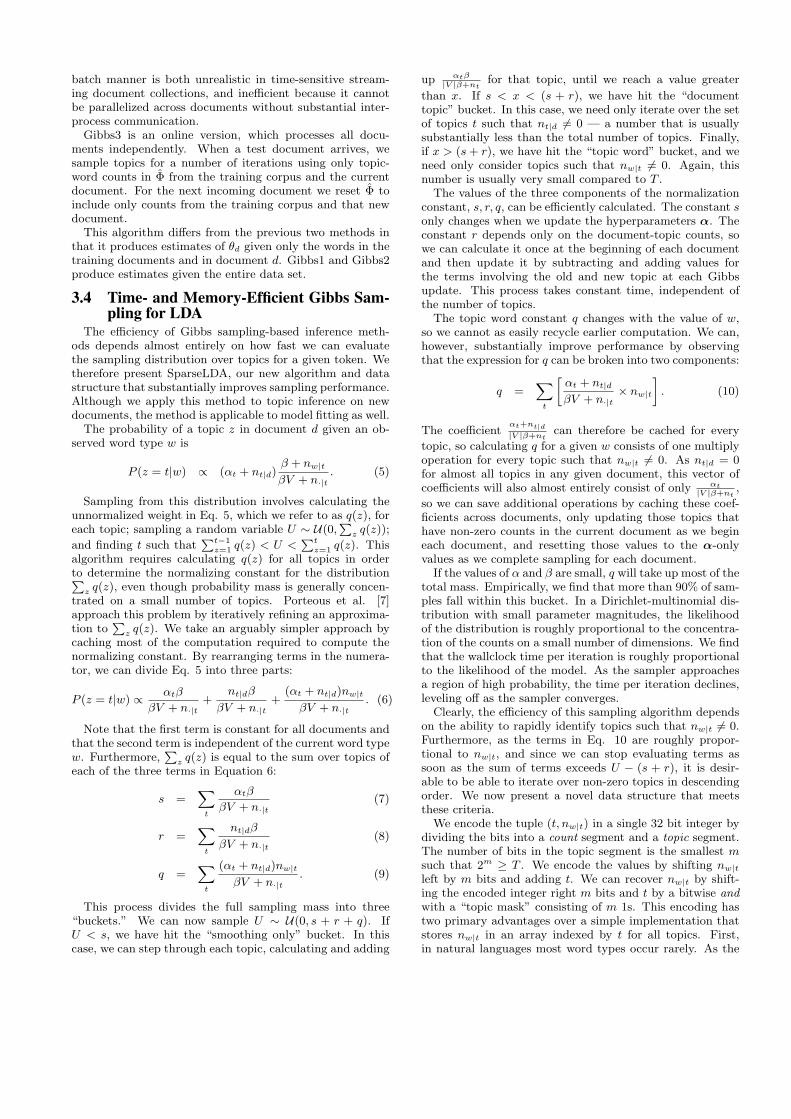
ods for LDA. Gibbs sampling is an MCMC method that in-volves iterating over a set of variables z1, z2, ...zn, samplingeach zi from P (zi|z\i, w). Each iteration over all variablesis referred to as a Gibbs sweep. Given enough iterations,Gibbs sampling for LDA [4] produces samples from the pos-terior P (z|w). The difference between the three methodswe explore is in the set of variables z that are sampled, asillustrated in Figure 1, and which portion of the completedata is used in estimating Φ.

3.1 Gibbs1: Jointly resample all topicsIn this method we define the scope of a single Gibbs sweep

to be the hidden topic variables for the entire collection,including both the original documents and the new docu-ments. After sampling the topic variables for the trainingdocuments to convergence without the new documents, werandomly initialize topic variables for the new documents

original training docs new docs

Gibbs1Gibbs2Gibbs3

Figure 1: The three Gibbs sampling-based methods it-

erate over a set of words, updating the topic assignment

for each word given the topic assignments for the remain-

ing words. The methods vary only in the set of topic

assignments they consider: Gibbs1 samples new topic

assignments for the entire corpus, including the origi-

nal training documents; Gibbs2 samples assignments for

only the new documents, holding the parameters for the

training corpus fixed; Gibbs3 samples each new docu-

ment independently.

and continue sampling over all documents until the modelconverges again. We can then estimate the topic distribu-tion θd for a given document given a single Markov chainstate as

θt|d =αt + nt|dPt′ αt′ + n·|d

, (4)

where n·|d is the length of the document. Increasingly ac-curate estimates can be generated by averaging over valuesof Eq. 4 for multiple Markov chain states, but may causeproblems due to label swapping.

Inference method Gibbs1 is equivalent to fitting a newmodel for the complete data, including both the originaldocuments and the new documents, after separately initial-izing some of the topic variables using Gibbs sampling. Thismethod is as computationally expensive as simply startingwith random initializations for all variables. It is useful,however, in that we can use the same initial model for allother inference methods, thereby ensuring that the topicswill roughly match up across methods. We consider thisinference procedure the most accurate, and the topic distri-bution for each test document estimated using Gibbs1 as areference for evaluating other inference methods.

3.2 Gibbs2: Jointly resample topics for all newdocuments

Inference method Gibbs2 begins with the same initializa-tion as Gibbs1, but saves computation by holding all of thetopic assignments for the training documents fixed. Underthis approximation, one Gibbs sweep only requires updatingtopic assignments for the new documents.

Inference involves sampling topic assignments for the train-ing data as in Gibbs1, randomly assigning values to the topicindicator variables z for the new documents, and then sam-pling as before, updating Φ as in Eq. 1 after each variableupdate.

3.3 Gibbs3: Independently resample topics fornew documents

Inference method Gibbs2 performs Gibbs sampling as abatch. As such, it samples from the posterior distributionover all z variables in the new documents given all the wordsin the new documents, accessing all the new documents ineach iteration. Unfortunately, handling topic inference in a

batch manner is both unrealistic in time-sensitive stream-ing document collections, and inefficient because it cannotbe parallelized across documents without substantial inter-process communication.

Gibbs3 is an online version, which processes all docu-ments independently. When a test document arrives, wesample topics for a number of iterations using only topic-word counts in Φ from the training corpus and the currentdocument. For the next incoming document we reset Φ toinclude only counts from the training corpus and that newdocument.

This algorithm differs from the previous two methods inthat it produces estimates of θd given only the words in thetraining documents and in document d. Gibbs1 and Gibbs2produce estimates given the entire data set.

3.4 Time- and Memory-Efficient Gibbs Sam-pling for LDA

The efficiency of Gibbs sampling-based inference meth-ods depends almost entirely on how fast we can evaluatethe sampling distribution over topics for a given token. Wetherefore present SparseLDA, our new algorithm and datastructure that substantially improves sampling performance.Although we apply this method to topic inference on newdocuments, the method is applicable to model fitting as well.

The probability of a topic z in document d given an ob-served word type w is

P (z = t|w) ∝ (αt + nt|d)β + nw|t

βV + n·|t. (5)

Sampling from this distribution involves calculating theunnormalized weight in Eq. 5, which we refer to as q(z), foreach topic; sampling a random variable U ∼ U(0,

Pz q(z));

and finding t such thatPt−1

z=1 q(z) < U <Pt

z=1 q(z). Thisalgorithm requires calculating q(z) for all topics in orderto determine the normalizing constant for the distributionP

z q(z), even though probability mass is generally concen-trated on a small number of topics. Porteous et al. [7]approach this problem by iteratively refining an approxima-tion to

Pz q(z). We take an arguably simpler approach by

caching most of the computation required to compute thenormalizing constant. By rearranging terms in the numera-tor, we can divide Eq. 5 into three parts:

P (z = t|w) ∝ αtβ

βV + n·|t+

nt|dβ

βV + n·|t+

(αt + nt|d)nw|t

βV + n·|t. (6)

Note that the first term is constant for all documents andthat the second term is independent of the current word typew. Furthermore,

Pz q(z) is equal to the sum over topics of

each of the three terms in Equation 6:

s =X

t

αtβ

βV + n·|t(7)

r =X

t

nt|dβ

βV + n·|t(8)

q =X

t

(αt + nt|d)nw|t

βV + n·|t. (9)

This process divides the full sampling mass into three“buckets.” We can now sample U ∼ U(0, s + r + q). IfU < s, we have hit the “smoothing only” bucket. In thiscase, we can step through each topic, calculating and adding

up αtβ|V |β+nt

for that topic, until we reach a value greater

than x. If s < x < (s + r), we have hit the “documenttopic” bucket. In this case, we need only iterate over the setof topics t such that nt|d 6= 0 — a number that is usuallysubstantially less than the total number of topics. Finally,if x > (s + r), we have hit the “topic word” bucket, and weneed only consider topics such that nw|t 6= 0. Again, thisnumber is usually very small compared to T .

The values of the three components of the normalizationconstant, s, r, q, can be efficiently calculated. The constant sonly changes when we update the hyperparameters α. Theconstant r depends only on the document-topic counts, sowe can calculate it once at the beginning of each documentand then update it by subtracting and adding values forthe terms involving the old and new topic at each Gibbsupdate. This process takes constant time, independent ofthe number of topics.

The topic word constant q changes with the value of w,so we cannot as easily recycle earlier computation. We can,however, substantially improve performance by observingthat the expression for q can be broken into two components:

q =X

t

»αt + nt|d

βV + n·|t× nw|t

–. (10)

The coefficientαt+nt|d|V |β+nt

can therefore be cached for every

topic, so calculating q for a given w consists of one multiplyoperation for every topic such that nw|t 6= 0. As nt|d = 0for almost all topics in any given document, this vector ofcoefficients will also almost entirely consist of only αt

|V |β+nt,

so we can save additional operations by caching these coef-ficients across documents, only updating those topics thathave non-zero counts in the current document as we begineach document, and resetting those values to the α-onlyvalues as we complete sampling for each document.

If the values of α and β are small, q will take up most of thetotal mass. Empirically, we find that more than 90% of sam-ples fall within this bucket. In a Dirichlet-multinomial dis-tribution with small parameter magnitudes, the likelihoodof the distribution is roughly proportional to the concentra-tion of the counts on a small number of dimensions. We findthat the wallclock time per iteration is roughly proportionalto the likelihood of the model. As the sampler approachesa region of high probability, the time per iteration declines,leveling off as the sampler converges.

Clearly, the efficiency of this sampling algorithm dependson the ability to rapidly identify topics such that nw|t 6= 0.Furthermore, as the terms in Eq. 10 are roughly propor-tional to nw|t, and since we can stop evaluating terms assoon as the sum of terms exceeds U − (s + r), it is desir-able to be able to iterate over non-zero topics in descendingorder. We now present a novel data structure that meetsthese criteria.

We encode the tuple (t, nw|t) in a single 32 bit integer bydividing the bits into a count segment and a topic segment.The number of bits in the topic segment is the smallest msuch that 2m ≥ T . We encode the values by shifting nw|tleft by m bits and adding t. We can recover nw|t by shift-ing the encoded integer right m bits and t by a bitwise andwith a “topic mask” consisting of m 1s. This encoding hastwo primary advantages over a simple implementation thatstores nw|t in an array indexed by t for all topics. First,in natural languages most word types occur rarely. As the

200 400 600 800

05000

15000

25000

Topics

Seconds/iteration

200 400 600 8000

100

200

300

400

Topics

Mem

ory

in M

B

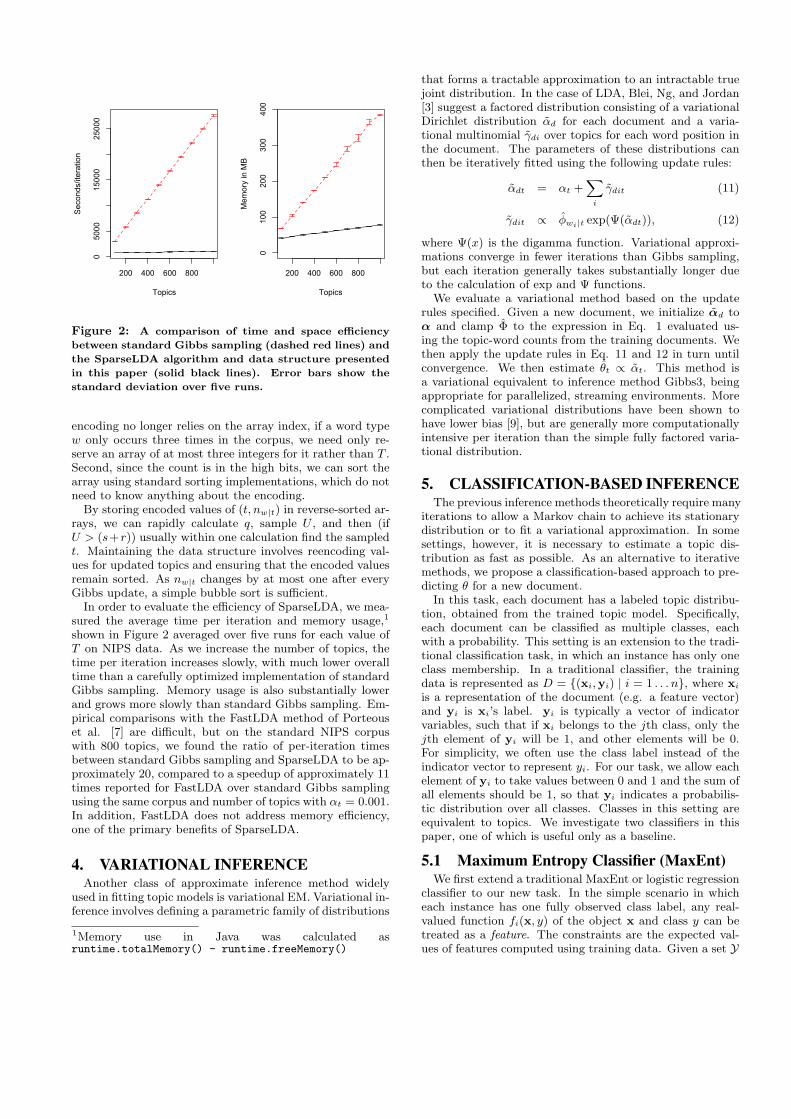
Figure 2: A comparison of time and space efficiency

between standard Gibbs sampling (dashed red lines) and

the SparseLDA algorithm and data structure presented

in this paper (solid black lines). Error bars show the

standard deviation over five runs.

encoding no longer relies on the array index, if a word typew only occurs three times in the corpus, we need only re-serve an array of at most three integers for it rather than T .Second, since the count is in the high bits, we can sort thearray using standard sorting implementations, which do notneed to know anything about the encoding.

By storing encoded values of (t, nw|t) in reverse-sorted ar-rays, we can rapidly calculate q, sample U , and then (ifU > (s+r)) usually within one calculation find the sampledt. Maintaining the data structure involves reencoding val-ues for updated topics and ensuring that the encoded valuesremain sorted. As nw|t changes by at most one after everyGibbs update, a simple bubble sort is sufficient.

In order to evaluate the efficiency of SparseLDA, we mea-sured the average time per iteration and memory usage,1

shown in Figure 2 averaged over five runs for each value ofT on NIPS data. As we increase the number of topics, thetime per iteration increases slowly, with much lower overalltime than a carefully optimized implementation of standardGibbs sampling. Memory usage is also substantially lowerand grows more slowly than standard Gibbs sampling. Em-pirical comparisons with the FastLDA method of Porteouset al. [7] are difficult, but on the standard NIPS corpuswith 800 topics, we found the ratio of per-iteration timesbetween standard Gibbs sampling and SparseLDA to be ap-proximately 20, compared to a speedup of approximately 11times reported for FastLDA over standard Gibbs samplingusing the same corpus and number of topics with αt = 0.001.In addition, FastLDA does not address memory efficiency,one of the primary benefits of SparseLDA.

4. VARIATIONAL INFERENCEAnother class of approximate inference method widely

used in fitting topic models is variational EM. Variational in-ference involves defining a parametric family of distributions

1Memory use in Java was calculated asruntime.totalMemory() - runtime.freeMemory()

that forms a tractable approximation to an intractable truejoint distribution. In the case of LDA, Blei, Ng, and Jordan[3] suggest a factored distribution consisting of a variationalDirichlet distribution αd for each document and a varia-tional multinomial γdi over topics for each word position inthe document. The parameters of these distributions canthen be iteratively fitted using the following update rules:

αdt = αt +X

i

γdit (11)

γdit ∝ φwi|t exp(Ψ(αdt)), (12)

where Ψ(x) is the digamma function. Variational approxi-mations converge in fewer iterations than Gibbs sampling,but each iteration generally takes substantially longer dueto the calculation of exp and Ψ functions.

We evaluate a variational method based on the updaterules specified. Given a new document, we initialize αd toα and clamp Φ to the expression in Eq. 1 evaluated us-ing the topic-word counts from the training documents. Wethen apply the update rules in Eq. 11 and 12 in turn untilconvergence. We then estimate θt ∝ αt. This method isa variational equivalent to inference method Gibbs3, beingappropriate for parallelized, streaming environments. Morecomplicated variational distributions have been shown tohave lower bias [9], but are generally more computationallyintensive per iteration than the simple fully factored varia-tional distribution.

5. CLASSIFICATION-BASED INFERENCEThe previous inference methods theoretically require many

iterations to allow a Markov chain to achieve its stationarydistribution or to fit a variational approximation. In somesettings, however, it is necessary to estimate a topic dis-tribution as fast as possible. As an alternative to iterativemethods, we propose a classification-based approach to pre-dicting θ for a new document.

In this task, each document has a labeled topic distribu-tion, obtained from the trained topic model. Specifically,each document can be classified as multiple classes, eachwith a probability. This setting is an extension to the tradi-tional classification task, in which an instance has only oneclass membership. In a traditional classifier, the trainingdata is represented as D = {(xi,yi) | i = 1 . . . n}, where xi

is a representation of the document (e.g. a feature vector)and yi is xi’s label. yi is typically a vector of indicatorvariables, such that if xi belongs to the jth class, only thejth element of yi will be 1, and other elements will be 0.For simplicity, we often use the class label instead of theindicator vector to represent yi. For our task, we allow eachelement of yi to take values between 0 and 1 and the sum ofall elements should be 1, so that yi indicates a probabilis-tic distribution over all classes. Classes in this setting areequivalent to topics. We investigate two classifiers in thispaper, one of which is useful only as a baseline.

5.1 Maximum Entropy Classifier (MaxEnt)We first extend a traditional MaxEnt or logistic regression

classifier to our new task. In the simple scenario in whicheach instance has one fully observed class label, any real-valued function fi(x, y) of the object x and class y can betreated as a feature. The constraints are the expected val-ues of features computed using training data. Given a set Y

of classes, and features fk, the parameters to be estimatedλk, the learned distribution p(y|x) is of the parametric ex-ponential form [2]:

P (y|x) =exp

`Pk λkfk(x, y)

´Py exp

`Pk λkfk(x, y)

´ . (13)

Given training data D = {〈x1, y1〉, 〈x2, y2〉, ..., 〈xn, yn〉}, thelog likelihood of parameters Λ is

l(Λ|D) = log

nY

i=1

p(yi|xi)

!−X

k

λ2k

2σ2

=

nXi=1

Xk

(λkfk(xi, yi)− log ZΛ(x))−X

k

λ2k

2σ2, (14)

The last term represents a zero-mean Gaussian prior on theparameters, which reduces overfitting and provides identifi-ability. We find values of Λ that maximize l(Λ|D) using astandard numerical optimizer. The gradient with respect tofeature index k is

δ(Λ|D)

δλk=

nXi=1

fk(xi, yi)−

Xy

fk(xi, y)p(y|xi)

!

− λk

σ2. (15)

In the topic distribution labeling task, each data pointhas a topic distribution, and is represented as (xi,yi). Wecan also use the maximum log likelihood method to solvethis model. The only required change is to substitute yfor y. Using a distribution changes the empirical featuresof the data (fk(xi, yi)), also known as the constraints ina maximum entropy model, which are used to compute thegradient. Whereas in a traditional classifier we use fk(xi, yi)as empirical features, we now use fk(xi,yi) instead, whereyi is the labeled topic distribution of the ith data point.Suppose that we have two classes (i.e. topics) and each in-stance can contain two features (i.e. words). Training datamight consist of x = (x1, x2), y = 1 for a traditional clas-sifier and x = (x1, x2),y = (p1, p2) for a topic distributionclassifier, such that p1 and p2 are the proportions of topic1 and topic 2 for data point x and p1 + p2 = 1. Empiricalfeatures (sufficient statistics of training data) for traditionalclassifier would be (x1, 1) and (x2, 1). While the empiricalfeatures for a topic distribution classifier would be (x1, 1),(x2, 1), (x1, 2), and (x2, 2), with the first two weighted byp1, and the remaining two weighted by p2. This substitutionchanges the penalized log likelihood function:

l(Λ | D) = log

nY

i=1

p(yi|xi)

!−X

k

λ2k

2σ2

=

nXi=1

Xk

(λkfk(xi,yi)− log ZΛ(x))−X

k

λ2k

2σ2, (16)

Correspondingly, the gradient at feature index k is:

δ(Λ|D)

δλk=

nXi=1

Xy

pi(y)fk(xi, y)−X

y

fk(xi, y)p(y|xi)

!

− λk

σ2. (17)

Where pi(y) stands for the probability of topic y in the cur-rent instance, i.e. one of the elements of yi.

Once we have trained a topic proportion classifier, we canuse it to estimate θ for a new document. We compute thescores for each topic using Eq. 13. This process is essentiallya table lookup for each word type, so generating θ requiresa single pass through the document.

In experiments, we found that the output of the topic pro-portion classifier is often overly concentrated on the singlelargest topic. We therefore introduce a temperature param-eter τ . Each feature value is weighted by 1

τ. Values of τ < 1

increase the peakiness of the classifier, while values τ > 1decrease peakiness. We chose 1.2 for NIPS data and 0.9for Pubmed data based on observation of the peakiness ofpredicted θ values for each corpus.

5.2 Naive Bayes ClassifierFrom the trained topic model, we can estimate Φ, a matrix

with T (#topics) rows and W (#words) columns represent-ing the probability of words given topics. Combined with auniform prior over topic distributions, we can use this ma-trix as a classifier, similar to the classifier we obtained fromMaxEnt. This method performs poorly, and is presentedonly as a baseline in our experiments. A document d isrepresented as a vector, with each element an entry in thevocabulary, denoted as w and the value as the number oftimes that word occurs in the document, denoted as nw|d.Using Bayes’ rule, the score for each topic is:

Score(z = t) =Xw

φw|tnw|d (18)

The estimated θ distribution is then simply the normalizedscores.

In experiments, we compare both classification methodsagainst the inference methods discussed in previous sections.The two classifiers take less time to predict topic distribu-tions, as they do not require iterative updates. Providedthey can achieve almost the same accuracy as the three in-ference methods or their performance is not much worse, forsome particular task which requires real-time response, wecan choose classification-based inference methods instead ofsampling based or variational updated methods. The choiceof estimator can be a trade-off between accuracy and timeefficiency.

5.3 Hybrid classification/sampling inferenceA hybrid classification/sampling-based approach can be

constructed by generating an estimate of θd given wd usingthe MaxEnt classifier and then repeatedly sampling topicindicators z given θ and Φ. Note that given θ, P (zi|wi) ∝θtφw|t is independent of all z\i. After the initial cost of set-ting up sampling distributions, sampling topic indicators foreach word can be performed in parallel and at minimal cost.After collecting sampled z indicators, we can re-estimate thetopic distribution θ according to the topic assignments as inEq. 4. In our experiments, we find that this re-sampling pro-cess results in more accurate topic distributions than Max-Ent alone.

6. EMPIRICAL RESULTSIn this section we empirically compare the relative accu-

racy of each inference method. We train a topic model ontraining data with a burn-in period of 1000 iterations forall inference methods. We explore the sensitivity of eachmethod to the number of topics, the proportion between

Table 1: Top five topics predicted by different meth-ods for a testing document

Method θt Highest probability words in topicGibbs1 0.4395 learning generalization error

0.2191 function case equation0.0734 figure time shown0.0629 information systems processing0.0483 training set data

MaxEnt 0.2736 learning generalization error0.2235 function case equation0.0962 figure time shown0.0763 information systems processing0.0562 learning error gradient

training documents and “new” documents, and the effect oftopic drift in new documents.

We evaluate different inference methods using two datasets. The first is 13 years of full papers published in theNIPS conference, in total 1,740 documents. The second isa set of 51,616 journal article abstracts from Pubmed. TheNIPS data set contains fewer documents, but each documentis longer. NIPS has around 70K unique words and 2.5Mtokens. Pubmed has around 105.4K unique words and about7M tokens. We also carried out experiments on New YorkTimes data from LDC. We used the first six months of 2007,comprising 39,218 documents, around 12M tokens, about900K unique words. We preprocessed the data by removingstop words.

We implemented the three sampling-based inference meth-ods (using SparseLDA), the variational updated method,and the classification-based methods in the MALLET toolkit[5]. They will be available as part of its standard open-sourcerelease.

6.1 Evaluation MeasuresIt is difficult to evaluate topic distribution prediction re-

sults, because the “true” topic distribution is unobservable.We can, however, compare different methods with each other.We consider the Gibbs1 inference method to be the most ac-curate, as it is closest to Gibbs sampling over the entire cor-pus jointly, a process that is guaranteed to produce samplesfrom the true posterior over topic distributions. In orderto determine whether sampling to convergence is necessary,for inference methods Gibbs2 and Gibbs3, we report resultsusing 1000 iterations of sampling (Gibbs2 and Gibbs3) andtwo iterations (Gibbs2.S and Gibbs3.S), which is the mini-mum number of Gibbs sweeps for all topic indicators to besampled using information from all other tokens.

We represent the prediction results of each method as aT -dimensional vector θd for each document. We comparemethods using three metrics. In all results we report theaverage of these measures over all “new” documents.

1. Cosine distance This metric measures the angle be-tween two vectors P and Q representing θd as esti-mated by two different inference methods:

Dcos(P‖Q) =

Pt ptqt

‖P‖‖Q‖ (19)

Values closer to 1.0 represent closely matched distri-butions.

2. KL Divergence Another metric between distribu-tions P and Q is KL divergence:

DKL(P‖Q) =X

t

pt logpt

qt. (20)

Smaller values of this metric represent closer distribu-tions. We use the “gold standard” inference methodas P .

3. F1 The previous two metrics measure the divergencebetween probability distributions. As shown in Ta-ble 1, however, it is common for estimators to pro-duce rather different distributions while maintainingroughly the same overall ordering of topics. In thismetric, we attempt to predict the set of topics thataccount for the largest probability mass. Specifically,we sort the entries in θd for a given inference methodin descending order and select a set of topics T suchthat

Pt∈T θtd ≤ 0.8. We can then treat TGibbs1 as

the correct topics and measure the precision and re-call of Tm for all other methods m. The F1 measure isthe harmonic mean between the precision and recall.Note that F1 does not take into account the order oftopics, only whether they are in the set of topics se-lected by the gold standard method. Values close to1.0 represent better matches.

For classification based inference methods we use unigramcounts as input features. Normalized term frequency fea-tures (term counts normalized by document length) pro-duced poorer results. We also tried including word-pairfeatures, on the intuition that the power of topic modelscomes from cooccurrence patterns in words, but these fea-tures greatly increased inference time, never improved re-sults over unigram features, and occasionally hurt perfor-mance. We hypothesize that the power of unigram featuresin the discriminatively trained MaxEnt classifier may bea result of the fact that the classifier can assign negativeweights to words as well as positive weights. This capabilityprovides extra power over the Naıve Bayes classifier, whichcannot distinguish between words that are strongly nega-tively indicative of a topic and words that are completelyirrelevant.

6.2 DiscussionWe first compare each method to the Gibbs1 inference

method, which is equivalent to completely retraining a modelgiven the original data and new data. We split the NIPSdata set into training and testing documents in a 7:3 ratioand run an initial model on the training documents with 70topics. We explore the effect of these settings later in thissection.

Figure 3 shows results for the three evaluation metrics.The converged sampling methods Gibbs2 and Gibbs3 areclosest to Gibbs1 in terms of cosine distance, F1, and KLdivergence, but do not exactly match. The two-iteration ver-sions Gibbs2.S and Gibbs3.S are close to Gibbs1 in terms ofcosine distance and KL divergence, but MaxEnt and Vari-ational EM are closer in terms of F1. Hybrid MaxEnt con-sistently outperforms MaxEnt. Figure 4 shows similar mea-sures vs. Gibbs2, arguably a more meaningful comparison

Gibbs1 Gibbs2 Gibbs3 MaxEnt NB

nips12/0286.txtTo

pic pr

opor

tion

0.00.2

0.40.6

0.81.0

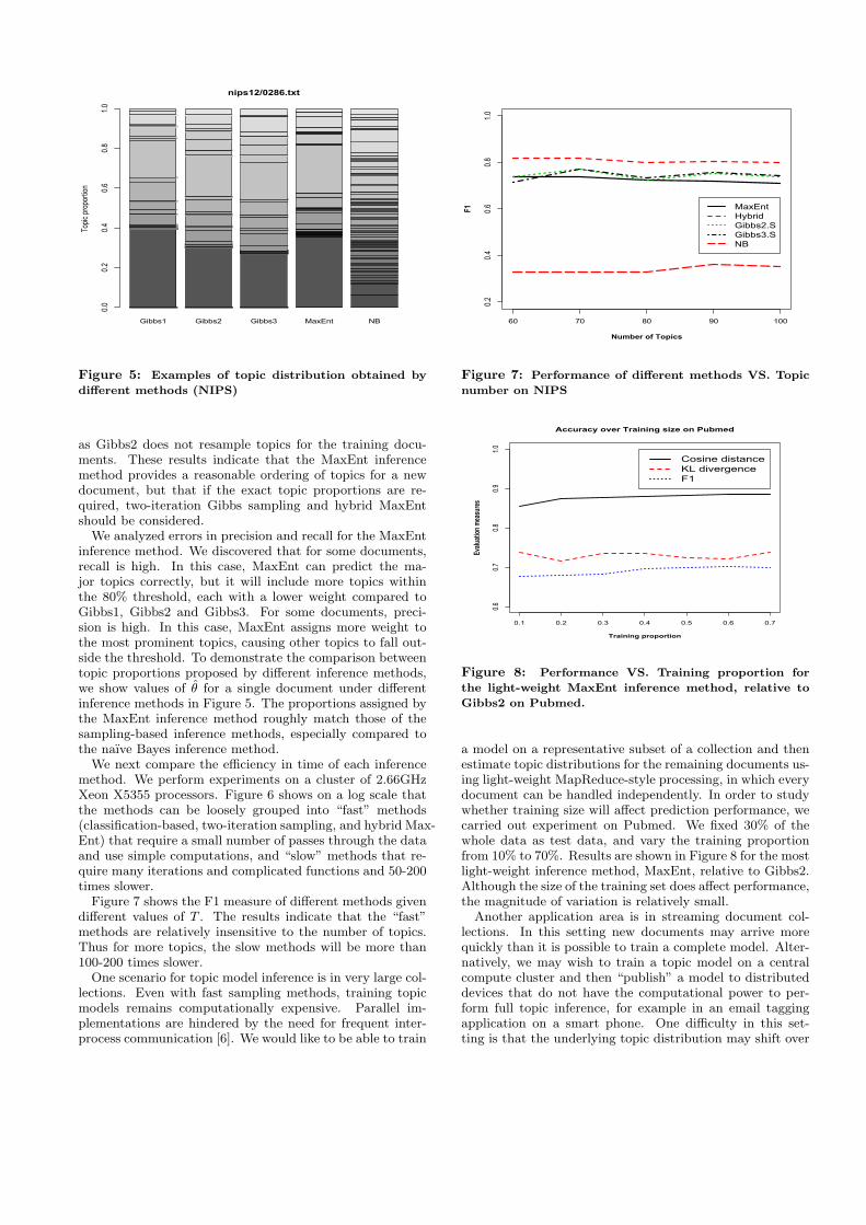
Figure 5: Examples of topic distribution obtained by

different methods (NIPS)

as Gibbs2 does not resample topics for the training docu-ments. These results indicate that the MaxEnt inferencemethod provides a reasonable ordering of topics for a newdocument, but that if the exact topic proportions are re-quired, two-iteration Gibbs sampling and hybrid MaxEntshould be considered.

We analyzed errors in precision and recall for the MaxEntinference method. We discovered that for some documents,recall is high. In this case, MaxEnt can predict the ma-jor topics correctly, but it will include more topics withinthe 80% threshold, each with a lower weight compared toGibbs1, Gibbs2 and Gibbs3. For some documents, preci-sion is high. In this case, MaxEnt assigns more weight tothe most prominent topics, causing other topics to fall out-side the threshold. To demonstrate the comparison betweentopic proportions proposed by different inference methods,we show values of θ for a single document under differentinference methods in Figure 5. The proportions assigned bythe MaxEnt inference method roughly match those of thesampling-based inference methods, especially compared tothe naıve Bayes inference method.

We next compare the efficiency in time of each inferencemethod. We perform experiments on a cluster of 2.66GHzXeon X5355 processors. Figure 6 shows on a log scale thatthe methods can be loosely grouped into “fast” methods(classification-based, two-iteration sampling, and hybrid Max-Ent) that require a small number of passes through the dataand use simple computations, and “slow” methods that re-quire many iterations and complicated functions and 50-200times slower.

Figure 7 shows the F1 measure of different methods givendifferent values of T . The results indicate that the “fast”methods are relatively insensitive to the number of topics.Thus for more topics, the slow methods will be more than100-200 times slower.

One scenario for topic model inference is in very large col-lections. Even with fast sampling methods, training topicmodels remains computationally expensive. Parallel im-plementations are hindered by the need for frequent inter-process communication [6]. We would like to be able to train

60 70 80 90 100

0.20.4

0.60.8

1.0

Number of Topics

F1 MaxEntHybridGibbs2.SGibbs3.SNB

Figure 7: Performance of different methods VS. Topic

number on NIPS

0.1 0.2 0.3 0.4 0.5 0.6 0.7

0.60.7

0.80.9

1.0

Accuracy over Training size on Pubmed

Training proportion

Evalu

ation

mea

sures

Cosine distanceKL divergenceF1

Figure 8: Performance VS. Training proportion for

the light-weight MaxEnt inference method, relative to

Gibbs2 on Pubmed.

a model on a representative subset of a collection and thenestimate topic distributions for the remaining documents us-ing light-weight MapReduce-style processing, in which everydocument can be handled independently. In order to studywhether training size will affect prediction performance, wecarried out experiment on Pubmed. We fixed 30% of thewhole data as test data, and vary the training proportionfrom 10% to 70%. Results are shown in Figure 8 for the mostlight-weight inference method, MaxEnt, relative to Gibbs2.Although the size of the training set does affect performance,the magnitude of variation is relatively small.

Another application area is in streaming document col-lections. In this setting new documents may arrive morequickly than it is possible to train a complete model. Alter-natively, we may wish to train a topic model on a centralcompute cluster and then “publish” a model to distributeddevices that do not have the computational power to per-form full topic inference, for example in an email taggingapplication on a smart phone. One difficulty in this set-ting is that the underlying topic distribution may shift over

Gibbs2 Gibbs3 Gibbs2.S Gibbs3.S VEM MaxEnt Hybrid NB

cosineF1

All methods compared with Gibbs1

0.0

0.2

0.4

0.6

0.8

1.0

Gibbs2 Gibbs3 Gibbs2.S Gibbs3.S VEM MaxEnt Hybrid NB

All methods compared with Gibbs1

KL D

iverg

ence

0.0

0.5

1.0

1.5

2.0

Figure 3: All methods compared with Gibbs1 on NIPS. Larger values are better in the left figure (cosine distance

and F1), while smaller KL divergences are better in the right figure.

Gibbs2.S Gibbs3.S MaxEnt Hybrid NB

cosineF1

Methods compared with Gibbs2

0.00.2

0.40.6

0.81.0

Gibbs2.S Gibbs3.S MaxEnt Hybrid NB

Methods compared with Gibbs2

KL D

iverge

nce

0.00.2

0.40.6

0.81.0

1.21.4

Figure 4: Methods compared with Gibbs2 on NIPS. Results for expensive iterative methods (Gibbs3, variational EM)

are not shown.

1 5 10 50 100 500 5000

0.0

0.2

0.4

0.6

0.8

1.0

Time (sec)

F1

Gibbs1Gibbs2Gibbs3MaxEntHybridNBGibbs2.SGibbs3.SVEM

1 5 10 50 100 500 5000

0.0

0.2

0.4

0.6

0.8

1.0

Time (sec)

Cos

ine

dist

ance

Gibbs1Gibbs2Gibbs3MaxEntHybridNBGibbs2.SGibbs3.SVEM

1 5 10 50 100 500 5000

0.0

0.5

1.0

1.5

2.0

Time (sec)

KL

Div

erge

nce

Gibbs1Gibbs2Gibbs3MaxEntHybridNBGibbs2.SGibbs3.SVEM

Figure 6: Performance of different methods VS. Time on NIPS

0.2 0.3 0.4 0.5 0.6 0.7 0.8 0.9

0.6

0.7

0.8

0.9

1.0

0.4

0.6

0.8

1.0

1.2

1.4

1.6

Jan

Jan-Feb

Jan-Mar

Jan-Apr

Jan-May

CosKLF1

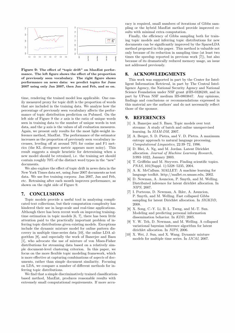
Figure 9: The effect of “topic drift” on MaxEnt perfor-

mance. The left figure shows the effect of the proportion

of previously seen vocabulary. The right figure shows

performance on news data: we predict topics for June

2007 using only Jan 2007, then Jan and Feb, and so on.

time, rendering the trained model less applicable. One eas-ily measured proxy for topic drift is the proportion of wordsthat are included in the training data. We analyze how thepercentage of previously seen vocabulary affects the perfor-mance of topic distribution prediction on Pubmed. On theleft side of Figure 9 the x axis is the ratio of unique wordsseen in training data to the number of unique words in testdata, and the y axis is the values of all evaluation measures.Again, we present only results for the most light-weight in-ference method, MaxEnt. The performance of the estimatorincreases as the proportion of previously seen vocabulary in-creases, leveling off at around 70% for cosine and F1 met-rics (the KL divergence metric appears more noisy). Thisresult suggests a simple heuristic for determining when anew model should be retrained, i.e. the training set shouldcontain roughly 70% of the distinct word types in the “new”documents.

We also explore the effect of topic drift in news data in theNew York Times data set, using June 2007 documents as testdata. We use five training corpora: Jan 2007, Jan and Feb,etc. Retraining after each month improves performance, asshown on the right side of Figure 9.

7. CONCLUSIONSTopic models provide a useful tool in analyzing compli-

cated text collections, but their computation complexity hashindered their use in large-scale and real-time applications.Although there has been recent work on improving training-time estimation in topic models [6, 7], there has been littleattention paid to the practically important problem of in-ferring topic distributions given existing models. Exceptionsinclude the dynamic mixture model for online pattern dis-covery in multiple time-series data [10], the online LDA al-gorithm [8], and especially the work of Banerjee and Basu[1], who advocate the use of mixture of von Mises-Fisherdistributions for streaming data based on a relatively sim-ple document-level clustering criterion. In this paper, wefocus on the more flexible topic modeling framework, whichis more effective at capturing combinations of aspects of doc-uments, rather than simple document similarity. Focusingon LDA, we compare a number of different methods for in-ferring topic distributions.

We find that a simple discriminatively trained classification-based method, MaxEnt, produces reasonable results withextremely small computational requirements. If more accu-

racy is required, small numbers of iterations of Gibbs sam-pling or the hybrid MaxEnt method provide improved re-sults with minimal extra computation.

Finally, the efficiency of Gibbs sampling both for train-ing topic models and inferring topic distributions for newdocuments can be significantly improved by the SparseLDAmethod proposed in this paper. This method is valuable notonly because of its reduction in sampling time (at least twotimes the speedup reported in previous work [7]), but alsobecause of its dramatically reduced memory usage, an issuenot addressed previously.

8. ACKNOWLEDGMENTSThis work was supported in part by the Center for Intel-

ligent Information Retrieval, in part by The Central Intel-ligence Agency, the National Security Agency and NationalScience Foundation under NSF grant #IIS-0326249, and inpart by UPenn NSF medium IIS-0803847. Any opinions,findings and conclusions or recommendations expressed inthis material are the authors’ and do not necessarily reflectthose of the sponsor.

9. REFERENCES[1] A. Banerjee and S. Basu. Topic models over text

streams: A study of batch and online unsupervisedlearning. In SIAM-DM, 2007.

[2] A. Berger, S. D. Pietra, and V. D. Pietra. A maximumentropy approach to natural language processing.Computational Linguistics, 22:39–72, 1996.

[3] D. Blei, A. Ng, and M. Jordan. Latent Dirichletallocation. Journal of Machine Learning Research,3:993–1022, January 2003.

[4] T. Griffiths and M. Steyvers. Finding scientific topics.PNAS, 101(Suppl. 1):5228–5235, 2004.

[5] A. K. McCallum. MALLET: A machine learning forlanguage toolkit. http://mallet.cs.umass.edu, 2002.

[6] D. Newman, A. Asuncion, P. Smyth, and M. Welling.Distributed inference for latent dirichlet allocation. InNIPS, 2007.

[7] I. Porteous, D. Newman, A. Ihler, A. Asuncion,P. Smyth, and M. Welling. Fast collapsed Gibbssampling for latent Dirichlet allocation. In SIGKDD,2008.

[8] X. Song, C.-Y. Li, B. L. Tseng, and M.-T. Sun.Modeling and predicting personal informationdissemination behavior. In KDD, 2005.

[9] Y. W. Teh, D. Newman, and M. Welling. A collapsedvariational bayesian inference algorithm for latentdirichlet allocation. In NIPS, 2006.

[10] X. Wei, J. Sun, and X. Wang. Dynamic mixturemodels for multiple time series. In IJCAI, 2007.