Efﬁcient ANOVA for directional data

Efficient ANOVA for directional data

Christophe Ley

Departement de Mathematique and ECARESUniversite Libre de BruxellesBoulevard du Triomphe, CP 210B-1050 Bruxelles, Belgium

Yvik Swan

Faculte des Sciences, de la Technologie et de la CommunicationUnite de Recherche en MathematiquesUniversite de Luxembourg6, rue Richard Coudenhove-KalergiL-1359 Luxembourg, Grand Duche de Luxembourg

Thomas Verdebout

EQUIPPEUniversite Lille Nord de FranceDomaine Universitaire du Pont de Bois, BP 60149F-59653 Villeneuve d’Ascq Cedex, France

Summary . In this paper we tackle the ANOVA problem for directional data (with particular em-phasis on geological data) by having recourse to the Le Cam methodology usually reserved forlinear multivariate analysis. We construct locally and asymptotically most stringent parametrictests for ANOVA for directional data within the class of rotationally symmetric distributions. Weturn these parametric tests into semi-parametric ones by (i) using a studentization argument(which leads to what we call pseudo-FvML tests) and by (ii) resorting to the invariance princi-ple (which leads to efficient rank-based tests). Within each construction the semi-parametrictests inherit optimality under a given distribution (the FvML distribution in the first case, anyrotationally symmetric distribution in the second) from their parametric antecedents and alsoimprove on the latter by being valid under the whole class of rotationally symmetric distri-butions. Asymptotic relative efficiencies are calculated and the finite-sample behavior of theproposed tests is investigated by means of a Monte Carlo simulation. We conclude by applyingour findings on a real-data example involving geological data.

1. Introduction

Spherical or directional data naturally arise in a broad range of earth sciences such asgeology, astrophysics, meteorology, oceanography, studies of animal behavior or even inneuroscience (see Mardia and Jupp 2000 or the recent Ley and Verdebout 2013 and therespective references therein). Although primitive statistical analysis of directional datacan already be traced back to early 19th century works by the likes of C. F. Gauss and

2 Ley et al. (2013)

D. Bernoulli, the methodical and systematic study of such non-linear data by means oftools tailored for their specificities only begun in the 1950s under the impetus of Sir RonaldFisher’s pioneering work (see Fisher 1953). We refer the reader to the monographs Fisheret al. (1987) and Mardia and Jupp (2000) for a thorough introduction and comprehensiveoverview of this discipline.

An important area of application of spherical statistics is in geology, in particularfor the study of palaeomagnetic data, see McFadden and Jones (1981), McFadden andLowes (1981), Fisher and Hall (1990) or the more recent Acton (2011). These data areusually modeled as realizations of random vectors X taking values on the surface of theunit hypersphere Sk−1 := {v ∈ R

k : v′v = 1}, the distribution of X depending only on itsangular distance from a fixed point θθθ ∈ Sk−1 which is to be viewed as a “north pole” forthe problem under study. A natural, flexible and realistic family of probability distribu-tions for such data is the class of so-called rotationally symmetric distributions introducedby Saw (1978) – see Section 2 below for definitions and notations. Roughly speaking suchdistributions allow to model all spherical data that are spread out uniformly around a cen-tral parameter θθθ with the concentration of the data waning as the angular distance fromthe north pole increases. This class of distributions contains, for instance, the most usedand best studied directional distribution: the so-called Fisher-von Mises-Langevin (FvML)distribution which will be defined in details in Section 2. Within this setup, an impor-tant question goes as follows : “do several measurements of remanent magnetization comefrom a same source of magnetism?” As recognized in the seminal paper Graham (1949),a positive answer to this question provides precious information about the stability of theremanence. Consequently, he developed the classical fold test for palaeomagnetic data; formore technical insights, see McFadden and Jones (1981) for the two-sample and McFaddenand Lowes (1981) for the multi-sample problem. In mathematical terms, the fold test can bedescribed as follows. Suppose that there are m different data sets spread around i sourcesof magnetism θθθi ∈ Sk−1, i = 1, . . . , m. The question then becomes that of testing for theproblem H0 : θθθ1 = . . . = θθθm against H1 : ∃ 1 ≤ i 6= j ≤ m such that θθθi 6= θθθj , that is, anANOVA problem for directional data. Of course, this problem is also of interest for theother above-mentioned branches dealing with directional observations.

Motivated by the fold test, the ANOVA problem has been largely studied in the statis-tical literature. The difficulty of the task, however, entails that most available methods areeither of parametric nature (assuming, as in McFadden and Jones 1981 and McFadden andLowes 1981, that the data follow a FvML distribution; see also Sections 10.5 and 10.6 ofMardia and Jupp 2000, where several FvML-based procedures are discussed), suffer fromcomputational difficulties/slowness (such as Wellner 1979’s permutation test or Fisher andHall 1990’s and Beran and Fisher 1998’s bootstrap test), lack desirable geometric proper-ties or are restricted to the circular (k = 2) setting (e.g., Eplett 1979 or Eplett 1982) orare confined to the two-sample case (e.g., Jupp 1987 or Tsai 2009). To the best of theauthor’s knowledge, the only semi-parametric, computationally simple, rotationally equiv-ariant, asymptotically distribution-free test for the general multisample null hypothesis H0

above is the test given in Watson (1983), which is most efficient under FvML assumptions.The purpose of the present paper thus is to complement this literature by constructing teststhat

(i) are optimal under a given m-tuple of distributions (P1, . . . , Pm) which need not be ofFvML type

(ii) do not assume that the Pi’s are all equal (thus allowing for distinct concentrations of

Efficient ANOVA for directional data 3

the data), and

(iii) remain valid (in the sense that they meet the nominal level constraint) under any m-tuple (Q1, . . . , Qm) satisfying the general null hypothesis H0 involving a large familyof spherical distributions.

In particular, the tests we propose are asymptotically distribution-free within the semi-parametric class of rotationally symmetric distributions. Obviously the applicability of ourANOVA procedures is not reserved to geological data alone, but directly extends to anytype of directional data for which the assumption of rotational symmetry with locationparameter θθθ seems to be reasonable.

The backbone of our approach is the so-called Le Cam methodology (see Le Cam 1986),as adapted to the spherical setup by Ley et al. (2013). Of utmost importance for ouraims here is the uniform local asymptotic normality (ULAN) of a sequence of rotationallysymmetric distributions established therein and which we adapt to our present purpose inSection 3. In the same Section 3 we also adapt results from Hallin et al. (2010) to determinethe general form of a so-called asymptotically most stringent parametric test for the abovehypothesis scheme H0 against H1. Due to its parametric nature the optimality of the(P1, . . . , Pm)-parametric test is thwarted by its non-validity under any m-tuple (Q1, . . . , Qm)distinct from (P1, . . . , Pm). In order to palliate this problem we have recourse to two classicaltools which we adapt to the spherical setting: first a studentization argument and secondthe invariance principle. While we apply the former method to the case where (P1, . . . , Pm)is a m-tuple of FvML distributions (due to their prominent role) leading to so-called pseudo-FvML tests, the latter method yields general (P1, . . . , Pm)-optimal rank-based tests. Bothfamilies of tests are of semi-parametric nature. Moreover, the Le Cam approach enables usto calculate the behavior of our tests under sequences of local alternatives, hereby allowingfor exact expressions of the powers of our tests.

While the construction of the tests is mathematically involved, the respective test statis-tics (4.8) and (5.10) have a concise form and are computationally simple. Therefore, forreaders preferring to skip the technicalities of Sections 3, 4 and 5, we briefly summarize inthe next two paragraphs the intricacies of our procedures.

The idea behind the pseudo-FvML test of Section 4 has the same flavor as the pseudo-Gaussian tests in the classical “linear” framework (see, for instance, Muirhead and Wa-ternaux 1980 or Hallin and Paindaveine 2008 for more information on pseudo-Gaussianprocedures). More concretely, since the FvML distribution is generally considered as thespherical analogue of the Gaussian distribution (see Section 2 for an explanation), our firstapproach consists in using the FvML as basis distribution and “correcting” the (parametric)FvML most stringent test, optimal under a m-tuple (P1, . . . , Pm) of FvML distributions, insuch a way that the resulting test φ(n) remains valid under the entire class of rotationallysymmetric distributions. We obtain the asymptotic distribution of the asymptotically moststringent pseudo-FvML test statistic Q(n) under the null and under contiguous alternatives.

As it turns out, the test statistic Q(n) and the test statistic Q(n)Watson provided in Watson

(1983) are asymptotically equivalent under the null (and therefore under contiguous alter-natives). As a direct consequence, we hereby obtain, in passing, that Watson (1983)’s test

φ(n)Watson also enjoys the property of being asymptotically most stringent in the FvML case.

The optimality property of φ(n)Watson and φ(n) is, by construction, restricted to situations

in which the underlying m-tuple of distributions is FvML. In Section 5 we therefore makeuse of the well-known invariance principle to construct a more flexible family of test statis-

4 Ley et al. (2013)

tics. To this end we first obtain a group of monotone transformations which generates thenull hypothesis. Then we construct tests based on the maximal invariant associated withthis group. The resulting tests (that are based on spherical signs and ranks) are, similarly

as φ(n)Watson and φ(n), asymptotically valid under any m-tuple of rotationally symmetric den-

sities. Our approach here, however, further entails that for any given m-tuple (P1, . . . , Pm)of rotationally symmetric distributions (not necessarily FvML ones) it suffices to choose theappropriate m-tuple K = (K1, . . . , Km) of score functions to guarantee that the resultingtest is asymptotically most stringent under (P1, . . . , Pm).

The more detailed outline of the paper is as follows. In Section 2, we define the classof rotationally symmetric distributions and collect the main assumptions of the paper.In Section 3, we summarize asymptotic results in the context of rotationally symmetricdistributions and show how to construct the announced optimal parametric tests for theANOVA problem. We then extend the latter to pseudo-FvML tests in Section 4 and to rank-based tests in Section 5, and study their respective asymptotic behavior in each section. Acomparison between both procedures on basis of asymptotic relative efficiencies as well asvia a Monte Carlo simulation study is provided in Section 6. We apply our findings on areal data application in Section 7. Finally an appendix collects the proofs.

2. Rotational symmetry

Throughout, the m(≥ 2) samples of data points Xi1, . . . ,Xini , i = 1, . . . , m, are assumedto belong to the unit sphere Sk−1 of R

k, k ≥ 2, and to satisfy

Assumption A. (Rotational symmetry) For all i = 1, . . . , m, Xi1, . . . ,Xini are i.i.d.with common distribution Pθθθi;fi

characterized by a density (with respect to the usual surfacearea measure on spheres)

x 7→ ck,fi fi(x′θθθi), x ∈ Sk−1, (2.1)

where θθθi ∈ Sk−1 is a location parameter, fi : [−1, 1] → R+0 is absolutely continuous and

(strictly) monotone increasing and ck,fi is a normalizing constant. Then, if X has density(2.1), the density of X′θθθi is of the form

t 7→ fi(t) :=ωk ck,fi

B(12 , 1

2 (k − 1))fi(t)(1 − t2)(k−3)/2, −1 ≤ t ≤ 1,

where ωk = 2πk/2/Γ(k/2) is the surface area of Sk−1 and B(·, ·) is the beta function. Thecorresponding cumulative distribution function (cdf) is denoted by Fi(t), i = 1, . . . , m.

The functions fi are called angular functions (because the distribution of each Xij de-pends only on the angle between it and the location θθθi ∈ Sk−1). Throughout the rest of thispaper, we denote by Fm the collection of m-tuples of angular functions f := (f1, f2, . . . , fm).Although not necessary for the definition to make sense, monotonicity of fi ensures thatsurface areas in the vicinity of the location parameter θθθi are allocated a higher proba-bility mass than more remote regions of the sphere. This property happens to be veryappealing from the modeling point of view. The assumption of rotational symmetry alsoentails appealing stochastic properties. Indeed, as shown in Watson (1983), for a randomvector X distributed according to some Pθθθi;fi

as in Assumption A, not only is the mul-tivariate sign vector Sθθθi

(X) := (X − (X′θθθi)θθθi)/||X − (X′θθθi)θθθi|| uniformly distributed on


Sθθθ⊥

i := {v ∈ Rk | ‖v‖ = 1,v′θθθi = 0} but also the angular distance X′θθθi and the sign vector

Sθθθi(X) are stochastically independent.The class of rotationally symmetric distributions contains a wide variety of useful spher-

ical distributions including the FvML, the spherical linear, the spherical logarithmic, thespherical logistic and the Purkayastha distributions (a definition of the latter four is providedin Section 6 below). The most popular and most used rotationally symmetric distributionis the aforementioned FvML distribution (named, according to Watson 1983, after vonMises 1918, Fisher 1953, and Langevin 1905), whose density is of the form

fFvML(κ)(x;θθθ) = ck(κ) exp(κx′θθθ), x ∈ Sk−1,

where κ > 0 is a concentration or dispersion parameter, θθθ ∈ Sk−1 a location parame-ter and ck(κ) is the corresponding normalizing constant. For ease of reference we shall,in what follows, rather use the notation φκ instead of fFvML(κ). This choice of nota-tion is motivated both by the wish for notational simplicity but also serves to furtherunderline the analogy between the FvML distribution as a spherical and the Gaussiandistribution as a linear distribution. This analogy is mainly due to the fact that theFvML distribution is the only spherical distribution for which the spherical empirical meanθθθMean :=

∑ni=1 Xi/||

∑ni=1 Xi|| (based on observations X1, . . . ,Xn ∈ Sk−1) is the Maximum

Likelihood Estimator (MLE) of its spherical location parameter, similarly as the Gaussiandistribution is the only (linear) distribution for which the empirical mean n−1

∑ni=1 Xi

(based on observations X1, . . . ,Xn ∈ Rk) is the MLE of the (linear) location parameter.

We refer the interested reader to Breitenberger (1963), Bingham and Mardia (1975) orDuerinckx and Ley (2013) for details and references on this topic; see also Schaeben (1992)for a discussion on spherical analogues of the Gaussian distribution.

3. ULAN and optimal parametric tests

Throughout this paper a test φ∗ is called optimal if it is most stringent for testing H0

against H1 within the class of tests Cα of level α, that is if

supP∈H1

rφ∗(P) ≤ supP∈H1

rφ(P) ∀φ ∈ Cα, (3.2)

where rφ0(P) stands for the regret of the test φ0 under P ∈ H1 defined as rφ0(P) :=[supφ∈Cα

EP[φ]]− EP[φ0], the deficiency in power of φ0 under P compared to the highest

possible (for tests belonging to Cα) power under P.As stated in the Introduction, the main ingredient for the construction of optimal (in

the sense of (3.2)) parametric tests for the null hypothesis H0 : θθθ1 = θθθ2 = . . . = θθθm consistsin establishing the ULAN property of the parametric model

({P

(n)θθθ1;f1

| θθθ1 ∈ Sk−1}

, . . . ,{P

(n)θθθm;fm

| θθθm ∈ Sk−1})

for a fixed m-tuple of (possibly different) angular functions f = (f1, . . . , fm), where P(n)θθθi;fi

stands for the joint distribution of Xi1, . . . ,Xini , i = 1, . . . , m, for a fixed m-tuple of angular

functions (f1, . . . , fm). Letting ϑϑϑ := (θθθ′1, . . . , θθθ′m)′, we further denote by P

(n)ϑϑϑ;f the joint law

combining P(n)θθθ1;f1

, . . . , P(n)θθθm;fm

. In order to be able to state our results, we need to impose acertain amount of control on the respective sample sizes ni, i = 1, . . . , m. This we achievevia the following

6 Ley et al. (2013)

Assumption B. Letting n =∑m

i=1 ni, for all i = 1, . . . , m the ratio r(n)i := ni/n converges

to a finite constant ri as n → ∞.

In particular Assumption B entails that the specific sizes ni are, up to a point, irrelevant;hence in what precedes and in what follows, we simply use the superscript (n) for thedifferent quantities at play and do not specify whether they are associated with a givenni. In the sequel we let diag(A1, . . . ,Am) stand for the m×m block-diagonal matrix with

blocks A1, . . . ,Am, and use the notation ννν(n) := diag((r(n)1 )−1/2Ik, . . . , (r

(n)m )−1/2Ik).

Informally, a sequence of rotationally symmetric models{

P(n)ϑϑϑ;f | ϑϑϑ ∈ (Sk−1)m

}is ULAN

if, uniformly in ϑϑϑ(n) = (θθθ(n)′1 , . . . , θθθ(n)′

m )′ ∈ (Sk−1)m such that ϑϑϑ(n) −ϑϑϑ = O(n−1/2), the log-likelihood ratio

log

(P

(n)

ϑϑϑ(n)+n−1/2ννν(n)t(n);f/P

(n)

ϑϑϑ(n);f

)

allows a specific form of (probabilistic) Taylor expansion (see equation (3.4) below) as a

function of t(n) := (t(n)′1 , . . . , t

(n)′m )′ ∈ R

mk. Of course the local perturbations t(n) must be

chosen so that ϑϑϑ(n) + n−1/2ννν(n)t(n) remains on (Sk−1)m and thus, in particular, the t(n)i

need to satisfy

0 = (θθθ(n)i + n

−1/2i t

(n)i )′(θθθ

(n)i + n

−1/2i t

(n)i ) − 1

= 2n−1/2i (θθθ

(n)i )′t

(n)i + n−1

i (t(n)i )′t

(n)i (3.3)

for all i = 1, . . . , m. Consequently, t(n)i must be such that 2n

−1/2i (θθθ

(n)i )′t

(n)i +o(n

−1/2i ) = 0 :

for θθθ(n)i + n

−1/2i t

(n)i to remain in Sk−1, the perturbation t

(n)i must belong, up to a o(n

−1/2i )

quantity, to the tangent space to Sk−1 at θθθ(n)i .

The domain of the parameter being the non-linear manifold(Sk−1

)mit is all but easy to

establish the ULAN property of a sequence of rotationally symmetric models. A natural wayto handle this difficulty consists, as in Ley et al. (2013), in resorting to a re-parameterizationof the problem in terms of spherical coordinates ηηη, say, for which it is possible to proveULAN, subject to the following technical condition on the angular functions.

Assumption C. The Fisher information associated with the spherical location parameteris finite; this finiteness is ensured if, for i = 1, . . . , m and letting ϕfi := fi/fi (fi is the

a.e.-derivative of fi), Jk(fi) :=∫ 1

−1ϕ2

fi(t)(1 − t2)fi(t)dt < +∞.

After obtaining the ULAN property for the ηηη-parameterization, one can use a lemma fromHallin et al. (2010) to transpose the ULAN property in the spherical ηηη-coordinates back interms of the original θθθ-coordinates. Finally the inner-sample independence and the mutualindependence between the m samples entail that we can deduce the required ULAN propertywhich is relevant for our purposes (this we state without proof because it follows directlyfrom Proposition 2.2 of Ley et al. 2013).

Proposition 3.1 Let Assumptions A, B and C hold. Then the model{

P(n)ϑϑϑ;f | ϑϑϑ ∈ (Sk−1)m

}


is ULAN with central sequence ∆∆∆(n)ϑϑϑ;f :=

((∆∆∆

(n)θθθ1;f1

)′, . . . , (∆∆∆(n)θθθm;fm

)′)′

, where

∆∆∆(n)θθθi;fi

:= n−1/2i

ni∑

j=1

ϕfi (X′ijθθθi)(1 − (X′

ijθθθi)2)1/2Sθθθi

(Xij), i = 1, . . . , m,

and Fisher information matrix ΓΓΓϑϑϑ;f := diag(ΓΓΓθθθ1;f1, . . . ,ΓΓΓθθθm;fm

) where

ΓΓΓθθθi;fi:=

Jk(fi)

k − 1(Ik − θθθiθθθ

′i), i = 1, . . . , m.

More precisely, for any ϑϑϑ(n) ∈ (Sk−1)m such that ϑϑϑ(n) − ϑϑϑ = O(n−1/2) and any bounded

sequences t(n) = (t(n)′1 , . . . , t

(n)′m )′ as in (3.3), we have

log

P(n)

ϑϑϑ(n)+n−1/2ννν(n)t(n);f

P(n)

ϑϑϑ(n);f

= (t(n))′∆∆∆

(n)

ϑϑϑ(n);f− 1

2(t(n))′ΓΓΓϑϑϑ;ft

(n) + oP(1), (3.4)

where ∆∆∆(n)

ϑϑϑ(n);f

L→ Nmk(000,ΓΓΓϑϑϑ;f ), both under P(n)ϑϑϑ;f , as n → ∞.

Proposition 3.1 provides us with all the necessary tools for building optimal f -parametricprocedures (i.e. under any m-tuple of densities with respective specified angular functionsf1, . . . , fm) for testing H0 : θθθ1 = . . . = θθθm against H1 : ∃ 1 ≤ i 6= j ≤ m such that θθθi 6= θθθj .Intuitively, this follows from the fact that the second-order expansion of the log-likelihood

ratio for the model{P

(n)ϑϑϑ;f | ϑϑϑ ∈ (Sk−1)m

}strongly resembles the log-likelihood ratio for the

classical Gaussian shift experiment, for which optimal procedures are well-known and arebased on the corresponding first-order term. Now clearly the null hypothesis H0 is theintersection between (Sk−1)m and the linear subspace (of R

mk)

C := {v = (v′1, . . . ,v

′m)′ |v1, . . . ,vm ∈ R

k and v1 = . . . = vm} =: M(1m ⊗ Ik)

where we put 1m := (1, . . . , 1)′ ∈ Rm, M(A) for the linear subspace spanned by the columns

of the matrix A and A⊗B for the Kronecker product between A and B. Such a restriction,namely an intersection between a linear subspace and a non-linear manifold, has alreadybeen considered in Hallin et al. (2010) in the context of Principal Component Analysis (inthat paper, the authors obtained very general results related to hypothesis testing in ULANfamilies with curved experiments). In particular from their results we can deduce that, inorder to obtain a locally and asymptotically most stringent test in the present context,one has to consider the locally and asymptotically most stringent test for the (linear) nullhypothesis defined by the intersection between C and the tangent to (Sk−1)m. Let θθθ denotethe common value of θθθ1, . . . , θθθm under the null. In the vicinity of 1m ⊗ θθθ, the intersectionbetween C and the tangent to (Sk−1)m is given by

{(θθθ′ + n−1/2(r

(n)1 )−1/2t

(n)′1 , . . . , θθθ′ + n−1/2(r

(n)m )−1/2t

(n)′m )′, (3.5)

θθθ′t(n)1 = . . . = θθθ′t

(n)m = 0, (r

(n)1 )−1/2t

(n)1 = . . . = (r

(n)m )−1/2t

(n)m

}.

Solving the system (3.5) yields

ννν(n)t(n) =((r

(n)1 )−1/2t

(n)′1 , . . . , (r(n)

m )−1/2t(n)′m

)′

∈ M(1m ⊗ (Ik − θθθθθθ′)). (3.6)

8 Ley et al. (2013)

Loosely speaking we have “transcripted” the initial null hypothesis H0 into a linear restric-tion of the form (3.6) in terms of local perturbations t(n), for which Le Cam’s asymptotictheory then provides a locally and asymptotically optimal parametric test under fixed f .

Using Proposition 3.1 and letting ΥΥΥϑϑϑ := 1m⊗ (Ik−θθθθθθ′) and ΥΥΥ(n)ϑϑϑ;ννν := (ννν(n))−1ΥΥΥϑϑϑ, an asymp-

totically most stringent test φf is then obtained by rejecting H0 as soon as (A− stands for

the Moore-Penrose pseudo-inverse of A)

Q(n)f := ∆∆∆′

ϑϑϑ;f

(ΓΓΓ−

ϑϑϑ;f −ΥΥΥ(n)ϑϑϑ;ννν

((ΥΥΥ

(n)ϑϑϑ;ννν)′ΓΓΓϑϑϑ;fΥΥΥ

(n)ϑϑϑ;ννν

)−

(ΥΥΥ(n)ϑϑϑ;ννν)′

)∆∆∆ϑϑϑ;f (3.7)

exceeds the α-upper quantile of a chi-square distribution with (m − 1)(k − 1) degrees offreedom. Hence the optimal parametric tests are now known.

There nevertheless remains much work to do. Indeed not only does the optimality of ourtest φf only hold under the m-tuple of angular densities f = (f1, . . . , fm), but also this para-

metric test suffers from the (severe) drawback of being only valid under that pre-specifiedm-tuple. Since it is highly unrealistic in practice to assume that the underlying densities areknown, these tests are useless for practitioners. Moreover, we so far have assumed knownthe common value of the spherical location under the null, which is unrealistic, too. Thenext two sections contain two distinct solutions allowing to set these problems right.

4. Pseudo-FvML tests

For a given m-tuple of FvML densities (φκ1 , . . . , φκm) with respective concentration param-eters κ1, . . . , κm > 0 (where we do not assume κ1 = . . . = κm), the score functions ϕφκi

reduce to the constants κi, i = 1, . . . , m, and hence the central sequences for each sampletake the simplified form

∆∆∆(n)θθθi;φκi

:= κin−1/2i

ni∑

j=1

(1 − (X′ijθθθi)

2)1/2Sθθθi(Xij)

= κin−1/2i

ni∑

j=1

(Xij − (X′ijθθθi)θθθi)

= κi(Ik − θθθiθθθ′i)n

−1/2i

ni∑

j=1

Xij

=: κi(Ik − θθθiθθθ′i)n

1/2i Xi

= κi(Ik − θθθiθθθ′i)n

1/2i (Xi − θθθi), i = 1, . . . , m.

Optimal FvML-based procedures (in the sense of (3.2)) for H0 are then built upon ∆∆∆(n)ϑϑϑ;φ =

(∆∆∆(n)′θθθ1;φκ1

, . . . ,∆∆∆(n)′θθθm;φκm

)′, where φ := (φκ1 , . . . , φκm).

Before proceeding we here again draw the reader’s attention to the fact that a parametric

test built upon ∆∆∆(n)ϑϑϑ;φ will only be valid under the m-tuple φ and becomes non-valid even

if only the concentration parameters change. In this section, this non-validity problemwill be overcome in the following way. We will first study the asymptotic behavior of

∆∆∆(n)ϑϑϑ;φ under any given m-tuple g = (g1, . . . , gm) ∈ Fm and consider the newly obtained


quadratic form in ∆∆∆(n)ϑϑϑ;φ. Clearly, this quadratic form will now depend on the asymptotic

variance of ∆∆∆(n)ϑϑϑ;φ under g, hence again, for each g, we are confronted to an only-for-g-

valid test statistic. The next step then consists in applying a studentization argument,meaning that we replace the asymptotic variance quantity by an appropriate estimator.We then study the asymptotic behavior of the new quadratic form under any m-tuple ofrotationally symmetric distributions. As we will show, the final outcome of this procedurewill be tests which happen to be optimal under any m-tuple of FvML distributions (thatis, for any values κ1, . . . , κm > 0) and valid under the entire class of rotationally symmetricdistributions; these tests are our so-called pseudo-FvML tests.

For the sake of readability, we adopt in the sequel the notations Ef [·] for expectationunder the angular function f and ϑϑϑ0 :=: 1m ⊗ θθθ (where we recall that θθθ represents thecommon value of θθθ1, . . . , θθθm under the null). The following result characterizes, for a givenm-tuple of angular functions g ∈ Fm, the asymptotic properties of the FvML-based central

sequence ∆∆∆(n)ϑϑϑ0;φ, both under P

(n)ϑϑϑ0;g and P

(n)

ϑϑϑ0+n−1/2ννν(n)t(n);gwith t(n) as in (3.3) for each

sample.

Proposition 4.1 Let Assumptions A, B and C hold. Then, letting Bk,gi := 1−Egi

[(X′

ijθθθ)2]

for i = 1, . . . , m, we have that ∆∆∆(n)ϑϑϑ0;φ is

(i) asymptotically normal under P(n)ϑϑϑ0;g

with mean zero and covariance matrix

ΓΓΓ∗ϑϑϑ0;g := diag

(ΓΓΓ∗

θθθ;g1, . . .ΓΓΓ∗

θθθ;gm

),

where ΓΓΓ∗θθθ;gi

:=κ2

i Bk,gi

k−1 (Ik − θθθθθθ′), i = 1, . . . , m;

(ii) asymptotically normal under P(n)

ϑϑϑ0+n−1/2ννν(n)t(n);g(t(n) as in (3.3)) with mean ΓΓΓϑϑϑ0;φ,gt

(t := (t′1, . . . , t′m)′ with ti := limn→∞ t

(n)i , i = 1, . . . , m) and covariance matrix ΓΓΓ∗

ϑϑϑ0;g,

where, putting Ck,gi := Egi [(1 − (X′ijθθθ)

2)ϕgi(X′ijθθθ)] for i = 1, . . . , m,

ΓΓΓϑϑϑ0;φ,g := diag(ΓΓΓθθθ;φκ1 ,g1

, . . . ,ΓΓΓθθθ;φκm ,gm

)

with ΓΓΓθθθ;φκi,gi

:=κiCk,gi

k−1 (Ik − θθθθθθ′), i = 1, . . . , m.

See the Appendix for the proof. As the null hypothesis only specifies that the sphericallocations coincide, we need to estimate the unknown common value θθθ. Therefore, we assumethe existence of an estimator θθθ of θθθ such that the following assumption holds.

Assumption D. The estimator ϑϑϑ = 1m ⊗ θθθ, with θθθ ∈ Sk−1, is n1/2(ννν(n)

)−1-consistent:

for all ϑϑϑ0 = 1m ⊗ θθθ ∈ H0, n1/2(ννν(n)

)−1(ϑϑϑ − ϑϑϑ0) = OP(1), as n → ∞ under P

(n)ϑϑϑ0;g for any

g ∈ Fm.

Typical examples of estimators satisfying Assumption D belong to the class of M -estimators

(see Chang 2004) or R-estimators (see Ley et al. 2013). Put simply, instead of ∆∆∆(n)ϑϑϑ0;φ

we

have to work with ∆∆∆(n)

ϑϑϑ;φfor some estimator ϑϑϑ satisfying Assumption D. The next crucial

result quantifies in how far this replacement affects the asymptotic properties establishedin Proposition 4.1 (a proof is provided in the Appendix).

10 Ley et al. (2013)

Proposition 4.2 Let Assumptions A, B and C hold and let ϑϑϑ = 1m ⊗ θθθ be an estimator ofϑϑϑ0 such that Assumption D holds. Then

(i) letting ΥΥΥ(n) :=

(√r(n)1 Ik

... . . ....

√r(n)m Ik

)′

, ∆∆∆(n)ϑϑϑ0;φ satisfies, under P

(n)ϑϑϑ0;g

and as n →∞,

∆∆∆(n)

ϑϑϑ;φ−∆∆∆

(n)ϑϑϑ0;φ

= −ΓΓΓφ

ϑϑϑ0;gΥΥΥ(n)√n

(θθθ − θθθ

)+ oP(1),

whereΓΓΓ

φ

ϑϑϑ0;g:= diag

(ΓΓΓ

φκ1

θθθ;g1, . . . ,ΓΓΓ

φκm

θθθ;gm

)

with ΓΓΓφκi

θθθ;gi:= κiEgi

[X′

ijθθθ](Ik − θθθθθθ′), i = 1, . . . , m;

ii) for all ϑϑϑ ∈ (Sk−1)m, ΓΓΓϑϑϑ;φ,φ = ΓΓΓφ

ϑϑϑ;φ = ΓΓΓ∗ϑϑϑ;φ.

Following the inspiration of Hallin and Paindaveine (2008) (where a very general theoryfor pseudo-Gaussian procedures is described) we are in a position to use Proposition 4.2to construct our pseudo-FvML tests. To this end define, for i = 1, . . . , m, the quantitiesEk,gi := Egi

[X′

ijθθθ], and set, for notational simplicity, Dk,gi := Ek,gi/Bk,gi and Hφ,g :=

∑mi=1 r

(n)i D2

k,giBk,gi . Then, letting

ΓΓΓ⊥ϑϑϑ0;φ,g := (ΓΓΓ∗

ϑϑϑ0;g)−

−(ΓΓΓ∗ϑϑϑ0;g)

−ΓΓΓφ

ϑϑϑ0;gΥΥΥ

(n)ϑϑϑ0;ννν [(ΥΥΥ

(n)ϑϑϑ0;ννν

)′ΓΓΓφ

ϑϑϑ0;g(ΓΓΓ∗

ϑϑϑ0;g)−ΓΓΓ

φ

ϑϑϑ0;gΥΥΥ

(n)ϑϑϑ0;ννν

]−(ΥΥΥ(n)ϑϑϑ0;ννν

)′ΓΓΓφ

ϑϑϑ0;g(ΓΓΓ∗ϑϑϑ0;g)

−

and Xi := n−1i

∑ni

j=1 Xij for all i = 1, . . . , m, the g-valid test statistic for H0 : θθθ1 = . . . = θθθm

we propose is the quadratic form

Q(n)(g) := (∆∆∆(n)

ϑϑϑ;φ)′ΓΓΓ⊥

ϑϑϑ;φ,g∆∆∆

(n)

ϑϑϑφ

= (k − 1)

m∑

i=1

niDk,gi

Ek,gi

X′i(Ik − θθθθθθ

′)Xi − (k − 1)

m∑

i,j

ninj

n

Dk,giDk,gj

Hφ,gX′

i(Ik − θθθθθθ′)Xj .

Note that Q(n)(g) does not depend explicitly on the underlying concentrations κ1, . . . , κm

but still depends on the quantities Bk,gi and Ek,gi , i = 1, . . . , m. This obviously hampersthe validity of the statistic outside of g. The last step thus consists in estimating thesequantities. Consistent (via the Law of Large Numbers) estimators for each of them are

provided by Bk,gi := 1−n−1i

∑ni

j=1(X′ijθθθ)

2 and Ek,gi := n−1i

∑ni

j=1(X′ijθθθ), i = 1, . . . , m. For

the sake of readability, we naturally also use the notations Dk,gi := Ek,gi/Bk,gi , i = 1, . . . , m,

and Hφ,g :=∑m

i=1 r(n)i D2

k,giBk,gi . Finally, the pseudo-FvML test statistic for the m-sample

spherical location problem is

Q(n) =(k − 1)

m∑

i=1

niDk,gi

Ek,gi


′)Xi − (k − 1)

m∑

i,j

ninj

n

Dk,giDk,gj

Hφ,g


′)Xj ,

(4.8)

which no more depends on g.The following proposition, whose proof is given in the Appendix, yields the asymptotic

properties of this quadratic form under the entire class of rotationally symmetric distribu-tions, showing that the test is well valid under that broad set of distributions.


Proposition 4.3 Let Assumptions A, B and C hold and let ϑϑϑ be an estimator of ϑϑϑ0 suchthat Assumption D holds. Then

(i) Q(n) is asymptotically chi-square with (m − 1)(k − 1) degrees of freedom under⋃ϑϑϑ0∈H0

⋃g∈Fm P

(n)ϑϑϑ0;g;

(ii) Q(n) is asymptotically non-central chi-square with k − 1 degrees of freedom and non-centrality parameter

lϑϑϑ0,t;φ,g := t′ΓΓΓϑϑϑ0;φ,gΓΓΓ⊥ϑϑϑ0;φ,gΓΓΓϑϑϑ0;φ,gt

under P(n)

ϑϑϑ0+n−1/2ννν(n)t(n);g, where t(n) is as in (3.3) and t := limn→∞ t(n);

(iii) the test φ(n) which rejects the null hypothesis as soon as Q(n) exceeds the α-upperquantile of the chi-square distribution with (m − 1)(k − 1) degrees of freedom has

asymptotic level α under⋃

ϑϑϑ0∈H0

⋃g∈Fm{P(n)

ϑϑϑ0;g};

(iv) φ(n) is locally and asymptotically most stringent, at asymptotic level α,

for⋃

ϑϑϑ0∈H0

⋃g∈Fm{P(n)

ϑϑϑ0;g} against alternatives of the form

⋃ϑϑϑ/∈H0

{P(n)ϑϑϑ;φ}.

It is easy to verify that Q(n) is asymptotically equivalent (the difference is a oP(1)quantity) to the test statistic for the same problem proposed in Watson (1983) under thenull (and therefore also under contiguous alternatives). Thus, although the construction wepropose is different, our pseudo-FvML tests coincide with Watson’s proposal. In passing,we have therefore also proved the asymptotic most stringency of the latter.

5. Rank-based tests

The pseudo-FvML test constructed in the previous section is valid under any m-tupleof (non-necessarily equal) rotationally symmetric distributions and retains the optimalityproperties of the FvML most stringent parametric test in the FvML case. Our aim in thepresent section is to provide tests which are optimal under any fixed (possibly non-FvML)m-tuple of rotationally symmetric distributions.

We start from any given m-tuple f ∈ Fm and our objective is to turn the f -parametrictests into tests which are still valid under any m-tuple of (non-necessarily equal) rotationallysymmetric distributions and which remain optimal under f . To obtain such a test, wehave recourse here to the second of the aforementioned tools to turn our parametric testsinto semi-parametric ones: the invariance principle. This principle advocates that, if thesub-model identified by the null hypothesis is invariant under the action of a group oftransformations GT , one should exclusively use procedures whose outcome does not changealong the orbits of that group GT . This is the case if and only if these procedures aremeasurable with respect to the maximal invariant associated with GT . The invarianceprinciple is accompanied by an appealing corollary for our purposes here: provided that thegroup GT is a generating group for H0, the invariant procedures are distribution-free underthe null.

Invariance with respect to “common rotations” is crucial in this context. More pre-cisely, letting O ∈ SOk := {A ∈ R

k×k,A′A = Ik, det(A) = 1}, the null hypothesis isunquestionably invariant with respect to a transformation of the form

gO : X11, . . . ,X1n1 , . . . ,Xm1, . . . ,Xmnm 7→ OX11, . . . ,OX1n1 , . . . ,OXm1, . . . ,OXmnm .

12 Ley et al. (2013)

However, this group is not a generating one for H0 as it does not take into account theunderlying angular functions f , which are an infinite-dimensional nuisance under H0. This

group is actually rather generating for⋃

ϑϑϑ0∈H0P

(n)ϑϑϑ0;f

with fixed f . Now, denote as in the

previous section the common value of θθθ1, . . . , θθθm under the null as θθθ. Then Xij = (X′ijθθθ)θθθ+√

1 − (X′ijθθθ)

2Sθθθ(Xij) for all j = 1, . . . , ni and i = 1, . . . , m. Let Gh (h := (h1, . . . , hm)) be

the group of transformations of the form

ghi : Xij 7→ ghi(Xij) = hi(X′ijθθθ)θθθ +

√1 − (hi(X′

ijθθθ))2Sθθθ(Xij), i = 1, . . . , m,

where the hi : [−1, 1] → [−1, 1] are monotone continuous nondecreasing functions suchthat hi(1) = 1 and hi(−1) = −1. For any m-tuple of (possibly different) transformations(gh1 , . . . , ghm) ∈ Gh, it is easy to verify that ‖ghi(Xij)‖ = 1; thus, ghi is a monotone trans-formation from Sk−1 to Sk−1, i = 1, . . . , m. Note furthermore that ghi does not modify the

signs Sθθθ(Xij). Hence the group of transformations Gh is a generating group for⋃

f∈Fm P(n)ϑϑϑ0;f

and the null is invariant under the action of Gh. Letting Rij denote the rank of X′ijθθθ among

X′i1θθθ, . . . ,X

′ini

θθθ, i = 1, . . . , m, it is now easy to conclude that the maximal invariant as-sociated with Gh is the vector of signs Sθθθ(X11), . . . ,Sθθθ(X1n1), . . . ,Sθθθ(Xm1), . . . ,Sθθθ(Xmnm)and ranks R11, . . . , R1n1 , . . . , Rm1, . . . , Rmnm .

As a consequence, we choose to base our tests in this section on a rank-based version of

the central sequence ∆∆∆(n)ϑϑϑ0;f

, namely on

∆∆∆˜

(n)ϑϑϑ0;K

:= ((∆∆∆˜

(n)θθθ;K1

)′, . . . , (∆∆∆˜

(n)θθθ;Km

)′)′

with

∆∆∆˜

(n)θθθ;Ki

= n−1/2i

ni∑

j=1

Ki

(Rij

ni + 1

)Sθθθ(Xij), i = 1, . . . , m,

where K := (K1, . . . , Km) is a m-tuple of score (generating) functions satisfying

Assumption E. The score functions Ki, i = 1, . . . , m, are continuous functions from [0, 1]to R.

The following result, which is a direct corollary (using again the inner-sample indepen-dence and the mutual independence between the m samples) of Proposition 3.1 in Ley et

al. (2013), characterizes the asymptotic behavior of ∆∆∆˜

(n)ϑϑϑ0;K

under any m-tuple of densitieswith respective angular functions g1, . . . , gm.

Proposition 5.1 Let Assumptions A, B, C and E hold and consider g = (g1, . . . , gm) ∈Fm. Then the rank-based central sequence ∆∆∆

˜(n)ϑϑϑ0;K

(i) is such that ∆∆∆˜

(n)ϑϑϑ0;K

−∆∆∆(n)ϑϑϑ0;K ;g = oP(1) under P

(n)ϑϑϑ0;g

as n → ∞, where (Gi standing for

the common cdf of the X′ijθθθ’s under P

(n)ϑϑϑ0;g, i = 1, . . . , m)

∆∆∆(n)ϑϑϑ0;K;g = ((∆∆∆

(n)θθθ;K1;g1

)′, . . . , (∆∆∆(n)θθθ;Km;gm

)′)′

with

∆∆∆(n)θθθ;Ki;gi

:= n−1/2i

ni∑

j=1

Ki

(Gi(X

′ijθθθ)

)Sθθθ(Xij), i = 1, . . . , m.


In particular, for K = Kf := (Kf1 , . . . , Kfm) with Kfi(u) := ϕfi(F−1i (u))(1 −

(F−1i (u))2)1/2, ∆∆∆

˜(n)ϑϑϑ0;Kf

is asymptotically equivalent to the efficient central sequence

∆∆∆(n)ϑϑϑ0;f under P

(n)ϑϑϑ0;f .

(ii) is asymptotically normal under P(n)ϑϑϑ0;g

with mean zero and covariance matrix

ΓΓΓϑϑϑ0;K := diag

(Jk(K1)

k − 1(Ik − θθθθθθ′), . . . ,

Jk(Km)

k − 1(Ik − θθθθθθ′)

),

where Jk(Ki) :=∫ 1

0K2

i (u)du.

(iii) is asymptotically normal under P(n)

ϑϑϑ0+n−1/2ννν(n)t(n);g(t(n) as in (3.3)) with mean ΓΓΓϑϑϑ0;K,gt

(t := limn→∞ t(n)) and covariance matrix

ΓΓΓϑϑϑ0;K,g := diag

(Jk(K1, g1)

k − 1(Ik − θθθθθθ′), . . . ,

Jk(Km, gm)


),

where Jk(Ki, gi) :=∫ 1

0Ki(u)Kgi(u)du for i = 1, . . . , m.

(iv) satisfies, under P(n)ϑϑϑ0;g

as n → ∞, the asymptotic linearity property

∆∆∆˜

(n)

ϑϑϑ0+n−1/2ννν(n)t(n);K− ∆∆∆

˜(n)ϑϑϑ0;K

= −ΓΓΓϑϑϑ0;K,gt(n) + oP(1),

for t(n) = (t(n)′1 , . . . , t

(n)′m )′ as in (3.3).

Similarly as for the pseudo-FvML test, our rank-based procedures are not completesince we still need to estimate the common value θθθ of θθθ1, . . . , θθθm under H0. To this end wewill assume the existence of an estimator ϑϑϑ satisfying the following strengthened version ofAssumption D :

Assumption D’. Besides n1/2(ννν(n)

)−1-consistency under P

(n)ϑϑϑ0;g

for any g ∈ Fm, the es-

timator ϑϑϑ ∈ (Sk−1)m is further locally and asymptotically discrete, meaning that it onlytakes a bounded number of distinct values in ϑϑϑ0-centered balls of the form {t ∈ R

mk :

n1/2‖(ννν(n)

)−1(t −ϑϑϑ0)‖ ≤ c}.

Estimators satisfying the above assumption are easy to construct. Indeed the consistencyis not a problem and the discretization condition is a purely technical requirement (neededto deal with these rank-based test statistics, see pages 125 and 188 of Le Cam and Yang 2000for a discussion) with little practical implications (in fixed-n practice, such discretizationsare irrelevant as the radius can be taken arbitrarily large). We will therefore tacitly assume

that θθθ ∈ Sk−1 (and therefore ϑϑϑ = 1m ⊗ θθθ) is locally and asymptotically discrete throughoutthis section. Following Lemma 4.4 in Kreiss (1987), the local discreteness allows to replacein Part (iv) of Proposition 5.1 non-random perturbations of the form ϑϑϑ+n−1/2ννν(n)t(n) witht(n) such that ϑϑϑ + n−1/2ννν(n)t(n) still belongs to H0 by a n1/2(ννν(n))−1-consistent estimator

ϑϑϑ := 1m ⊗ θθθ. Based on the asymptotic result of Proposition 5.1 and letting

ΓΓΓ⊥ϑϑϑ0;K,g := ΓΓΓ−

ϑϑϑ0;K

−ΓΓΓ−ϑϑϑ0;KΓΓΓϑϑϑ0;K,gΥΥΥ

(n)ϑϑϑ0;ννν

[(ΥΥΥ(n)ϑϑϑ0;ννν)′ΓΓΓϑϑϑ0;K,gΓΓΓ

−ϑϑϑ0;K

ΓΓΓϑϑϑ0;K,gΥΥΥ(n)ϑϑϑ0;ννν

]−(ΥΥΥ(n)ϑϑϑ0;ννν)′ΓΓΓϑϑϑ0;K,gΓΓΓ

−ϑϑϑ0;K

,

14 Ley et al. (2013)

the g-valid rank-based test statistic we propose for the present ANOVA problem correspondsto the quadratic form

QK(g)(n) := (∆∆∆˜

(n)

ϑϑϑ;K)′ΓΓΓ⊥

ϑϑϑ;K,g∆∆∆˜

(n)

ϑϑϑ;K.

This test statistic still depends on the cross-information quantities

Jk(Kf1 , g1), . . . ,Jk(Kfm , gm) (5.9)

and hence is only valid under fixed g. Therefore, exactly as for the pseudo-FvML tests of theprevious section, the final step in our construction consists in estimating these quantitiesconsistently. For this define, for any ρ ≥ 0,

θθθi(ρ) := θθθ + n−1/2i ρ (k − 1)(Ik − θθθθθθ

′)∆∆∆

˜(n)

θθθ;Ki, i = 1, . . . , m.

Then, letting θθθi(ρ) := θθθi(ρ)/‖θθθi(ρ)‖, we consider the piecewise continuous quadratic form

ρ 7→ h(n)i (ρ) :=

k − 1

J (Ki)(∆∆∆

˜(n)

θθθ;Ki)′ ∆∆∆

˜(n)

θθθi(ρ);Ki.

Consistent estimators of the quantities J−1k (K1, g1), . . . ,J −1

k (Km, gm) (and therefore read-ily of (5.9)) can be obtained by taking

ρi := inf{ρ > 0 : h(n)i (ρ) < 0}

for i = 1, . . . , m (see also Ley et al. 2013 for more details). Denoting by Jk(Ki, gi), for

i = 1, . . . , m, the resulting estimators, setting HK,g :=∑m

i=1 r(n)i J 2

k (Ki, gi)/Jk(Ki) and

letting Uij := Ki

(Rij/(ni + 1)

)Sθθθ(Xij), i = 1, . . . , m, (Rij naturally stands for the rank

of X′ijθθθ among X′

i1θθθ, . . . ,X′ini

θθθ), the proposed rank test φ˜

(n)K rejects the null hypothesis of

homogeneity of the locations when

Q˜

(n)K := (k − 1)

m∑

i=1

ni

Jk(Ki)U′

iUi − (k − 1)H−1K,g

m∑

i,j=1

ninj

n

Jk(Ki, gi)

Jk(Ki)

Jk(Kj , gj)

Jk(Kj)U′

iUj

(5.10)

exceeds the α-upper quantile of the chi-square distribution with (m − 1)(k − 1) degreesof freedom. This asymptotic behavior under the null as well as the asymptotic distribu-

tion of Q˜

(n)K under a sequence of contiguous alternatives are summarized in the following

proposition.

Proposition 5.2 Let Assumptions A, B, C and E hold and let ϑϑϑ be an estimator such thatAssumption D’ holds. Then

(i) Q˜

(n)K is asymptotically chi-square with (m − 1)(k − 1) degrees of freedom under

⋃ϑϑϑ0∈H0

⋃g∈Fm{P(n)

ϑϑϑ0;g};

(ii) Q˜

(n)K is asymptotically non-central chi-square, still with (m − 1)(k − 1) degrees of

freedom, but with non-centrality parameter

lϑϑϑ0,t;K,g := t′ΓΓΓϑϑϑ0;K,gΓΓΓ⊥ϑϑϑ0;K,gΓΓΓϑϑϑ0;K,gt

under P(n)

ϑϑϑ0+n−1/2ννν(n)t(n);g, where t(n) is as in (3.3) and t := limn→∞ t(n);


(iii) the test φ˜

(n)K which rejects the null hypothesis as soon as Q

˜(n)K exceeds the α-upper

quantile of the chi-square distribution with (m − 1)(k − 1) degrees of freedom has

asymptotic level α under⋃

ϑϑϑ0∈H0

⋃g∈Fm{P(n)

ϑϑϑ0;g};

(iv) in particular, for K = Kf := (Kf1 , . . . , Kfm) with Kfi(u) := ϕfi(F−1i (u))(1 −

(F−1i (u))2)1/2, φ

˜(n)Kf

is locally and asymptotically most stringent, at asymptotic level α,

for⋃

ϑϑϑ0∈H0

⋃g∈Fm{P(n)

ϑϑϑ0;g} against alternatives of the form

⋃ϑϑϑ/∈H0

{P(n)ϑϑϑ;f}.

Thanks to Proposition 5.1, the proof of this result follows along the same lines as that ofProposition 4.3 and is therefore omitted.

6. Comparison of the proposed test procedures

In what follows, we will compare the optimal pseudo-FvML test (hence, the Watson test)

φ(n) to optimal rank-based tests φ˜

(n)Kf

for several choices of f ∈ Fm, both at asymptotic

level via the calculation of Pitman’s asymptotic relative efficiencies (AREs, Section 6.1) andat finite-sample level via a Monte Carlo simulation study (Section 6.2).

6.1. Asymptotic relative efficienciesLet AREϑϑϑ0;g(φ

(n)1 , φ

(n)2 ) denote the ARE of a test φ

(n)1 with respect to another test φ

(n)2

under P(n)

ϑϑϑ0+n−1/2ννν(n)t(n);g. Thanks to Propositions 4.3 and 5.2, we find that

AREϑϑϑ0;g(φ˜

(n)Kf

, φ(n)) = lϑϑϑ0,t;Kf ,g/lϑϑϑ0,t;φ,g. (6.11)

In the homogeneous case g = (g1, . . . , g1) (the angular density is the same for the m sam-ples) and if the same score function—namely, Kf1—is used for the m rankings (the test is

therefore denoted by φ˜

(n)Kf1

), the ratio in (6.11) simplifies into

AREϑϑϑ0;g(φ˜(n)Kf1

/φ(n)) =J 2

k (Kf1 , g1)Bk,g1

Jk(Kf1)C2k,g1

. (6.12)

Numerical values of the AREs in (6.12) are reported in Table 1 for the three-dimensionalsetup under various angular densities and various choices of the score function Kf1 . Moreprecisely, besides the FvML we consider the spherical linear, logarithmic, logistic andsquared distributions with respective angular functions

flin(a)(t) := t + a, flog(a)(t) := log(t + a)

flogis(a,b)(t) :=a exp(−b arccos(t))

(1 + a exp(−b arccos(t)))2and fSq(a)(t) =

√t + a.

The constants a and b are chosen so that all the above functions are true angular functionssatisfying Assumption A. The score functions associated with all these angular functionsare denoted by Klin(a) for flin(a), Klog(a) for flog(a), Klogis(a,b) for flogis(a,b) and KSq(a) for

16 Ley et al. (2013)

Table 1. Asymptotic relative efficiencies of (homogeneous) rank-based tests φe

(n)Kf1

with respect to the pseudo-

FvML test φ(n) under various three-dimensional rotationally symmetric densities.

ARE(φe

(n)Kf1

/φ(n))

Underlying density φe

(n)Kφ2

φe

(n)Kφ6

φe

(n)Klin(2)

φe

(n)Klin(4)

φe

(n)Klog(2.5)

φe

(n)Klogis(1,1)

φe

(n)KSq(2)

FvML(1) 0.9744 0.8787 0.9813 0.9979 0.9027 0.9321 0.9992FvML(2) 1 0.9556 0.9978 0.9586 0.9749 0.9823 0.9919FvML(6) 0.9555 1 0.9381 0.8517 0.9768 0.9911 0.9154Lin(2) 1.0539 0.9909 1.0562 1.0215 1.0212 1.0247 1.0531Lin(4) 0.9709 0.8627 0.9795 1.0128 0.8856 0.9231 0.9957

Log(2.5) 1.1610 1.1633 1.1514 1.0413 1.1908 1.1625 1.1252Log(4) 1.0182 0.9216 1.0261 1.0347 0.9503 0.9741 1.0359

Logis(1,1) 1.0768 1.0865 1.0635 0.9991 1.0701 1.0962 1.0485Logis(2,1) 1.3182 1.4426 1.2946 1.0893 1.4294 1.3865 1.2411Sq(1.1) 1.2303 1.3460 1.1964 1.0264 1.3158 1.3004 1.1478Sq(2) 1.0502 0.9692 1.0556 1.0408 1.0003 1.0127 1.0587

fSq(a). For the FvML distribution with concentration κ, the score function will be denotedby Kφκ .

Inspection of Table 6.1 confirms the theoretical results. As expected, the pseudo-FvMLtest φ(n) dominates the rank-based tests under FvML densities, whereas rank-based testsmostly outperform the pseudo-FvML test under other densities, especially so when theyare based on the score function associated with the underlying density (in which case therank-based tests are optimal).

6.2. Monte Carlo simulation resultsIn order to study the finite-sample behavior of the pseudo-FvML test φ(n) and various rank-

based tests φ˜

(n)Kf

, we have conducted a Monte Carlo simulation study on R for moderate,

small and very small sample sizes for the two-sample spherical location problem, that is,for an ANOVA with m = 2.

6.2.1. First setting: moderate sample sizes

We generated M = 1, 500 replications of five pairs of mutually independent samples (withrespective sizes n1 = 200 and n2 = 250) of (k =)3-dimensional rotationally symmetricrandom vectors

εεεℓ;iji , ℓ = 1, 2, 3, 4, 5, ji = 1, . . . , ni, i = 1, 2,

with FvML densities, linear densities and Purkayastha densities (the Purkayastha 1991distribution is associated with angular functions of the form fPur(a)(t) = e−a arccos(t), a > 0):the εεε1;1j1 ’s have a FvML(5) distribution and the εεε1;2j2 ’s have a FvML(2) distribution; theεεε2;1j1 ’s have a Lin(5) distribution and the εεε2;2j2 ’s have a Lin(2) distribution; the εεε3;1j1 ’shave a FvML(5) distribution and the εεε3;2j2 ’s have a Lin(2) distribution; the εεε4;1j1 ’s have aPur(.2) distribution and the εεε4;2j2 ’s have a Pur(.4) distribution and finally the εεε5;1j1 ’s havea FvML(5) distribution and the εεε5;2j2 ’s have a Pur(.4) distribution.


The rotationally symmetric vectors εεεℓ;iji ’s have all been generated with a common spher-ical location θθθ0 = (1, 0, 0)′. Then, each replication of the εεεℓ;iji ’s was transformed into

{Xℓ;1j1 = εεεℓ;1j1 , ℓ = 1, 2, 3, 4, 5 j1 = 1, . . . , n1

Xℓ;2j2;ξ = Oξεεεℓ;2j2 , ℓ = 1, 2, 3, 4, 5 j2 = 1, . . . , n2, ξ = 0, 1, 2, 3,

where

Oξ =

cos(πξ/15) − sin(πξ/15) 0sin(πξ/15) cos(πξ/15) 0

0 0 1

.

Clearly, the spherical locations of the Xℓ;1j1 ’s and the Xℓ;2j2;0’s coincide while the spher-ical location of the Xℓ;2j2;ξ’s, ξ = 1, 2, 3, is different from the spherical location of theXℓ;1j1 ’s, characterizing alternatives to the null hypothesis of common spherical locations.Rejection frequencies based on the asymptotic chi-square critical values at nominal level 5%are reported in Table 2 below.

6.2.2. Second setting: small sample sizes

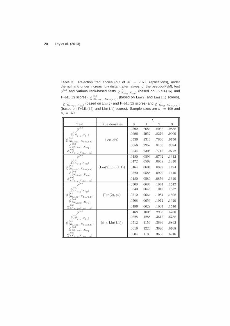
In this subsection, we generated M = 2, 500 replications of four pairs of mutually inde-pendent samples (with respective sizes n1 = 100 and n2 = 150) of (k =)3-dimensionalrotationally symmetric random vectors

εεεℓ;iji , ℓ = 1, 2, 3, 4, ji = 1, . . . , ni, i = 1, 2,

with FvML densities and linear densities: the εεε1;1j1 ’s have a FvML(15) distribution and theεεε1;2j2 ’s have a FvML(2) distribution; the εεε2;1j1 ’s have a Lin(2) distribution and the εεε2;2j2 ’shave a Lin(1.1) distribution; the εεε3;1j1 ’s have a FvML(15) distribution and the εεε3;2j2 ’s havea Lin(1.1) distribution and finally the εεε4;1j1 ’s have a Lin(2) distribution and the εεε4;2j2 ’shave a FvML(2) distribution.

The rotationally symmetric vectors εεεℓ;iji ’s have all been generated with a common spher-ical location θθθ0 = (

√3/2, 1/2, 0)′. Then, each replication of the εεεℓ;iji ’s was transformed into

{Xℓ;1j1 = εεεℓ;1j1 , ℓ = 1, 2, 3, 4, j1 = 1, . . . , n1

Xℓ;2j2;ξ = Oξεεεℓ;2j2 , ℓ = 1, 2, 3, 4, j2 = 1, . . . , n2, ξ = 0, 1, 2, 3,

where

Oξ =


0 0 1

.

As previously, the spherical locations of the Xℓ;1j1 ’s and the Xℓ;2j2;0’s coincide while thespherical location of the Xℓ;2j2;ξ’s, ξ = 1, 2, 3, is different from the spherical location of theXℓ;1j1 ’s, characterizing alternatives to the null hypothesis of common spherical locations.Rejection frequencies based on the asymptotic chi-square critical values at nominal level 5%are reported in Table 3 below.

6.2.3. Third setting: really small sample sizes

In this subsection, we generated M = 1, 500 replications of two pairs of mutually inde-pendent samples (with sizes n1 = n2 = 30) of (k =)3-dimensional rotationally symmetricrandom vectors

εεεℓ;iji , ℓ = 1, 2, ji = 1, . . . , ni, i = 1, 2,

18 Ley et al. (2013)

with FvML densities and linear densities: the εεε1;1j1 ’s and the εεε1;2j2 ’s have a FvML(1) distri-bution; the εεε2;1j1 ’s have a FvML(1) distribution and the εεε2;2j2 ’s have a Lin(5) distribution.

The rotationally symmetric vectors εεεℓ;iji ’s have all been generated with a common spher-ical location θθθ0 = (1, 0, 0)′. Then, each replication of the εεεℓ;iji ’s was transformed into

{Xℓ;1j1 = εεεℓ;1j1 , ℓ = 1, 2, j1 = 1, . . . , n1

Xℓ;2j2;ξ = Oξεεεℓ;2j2 , ℓ = 1, 2, j2 = 1, . . . , n2, ξ = 0, 1, 2, 3,

where

Oξ =


0 0 1

.

Once again, the spherical locations of the Xℓ;1j1 ’s and the Xℓ;2j2;0’s coincide while thespherical location of the Xℓ;2j2;ξ’s, ξ = 1, 2, 3, is different from the spherical location of theXℓ;1j1 ’s, characterizing alternatives to the null hypothesis of common spherical locations.Power curves based on the asymptotic chi-square critical values at nominal level 5% areplotted in Figure 1 below.

6.2.4. Conclusions

The inspection of Tables 2 and 3 and of Figure 1 reveals nice results:

(i) The pseudo-FvML test and all the rank-based tests are valid under heterogeneousdensities. They reach the 5% nominal level constraint under any considered pair ofdensities.

(ii) The comparison of the empirical powers reveals that when based on scores associatedwith the underlying distributions, the rank-based tests are quite powerful.

(iii) The proposed procedures (even the rank-based tests) perform surprisingly well under(very) small sample sizes.

7. Real-data example

In this section, we apply our new tests on a real-data example. The data consist of measure-ments of remanent magnetization in red slits and claystones made at 2 different locationsin Eastern New South Wales, Australia, the first location yielding n1 = 39, the secondn2 = 36 observations; see Embleton and McDonnell (1980) for details. As can be seen fromFigure 2, the rotational symmetry assumption in the two samples seems to be appropriatesince data are clearly concentrated. However, the specification of the angular functions isnot reasonable, whence our semi-parametric procedures are quite useful in this setting.

As explained in the Introduction, the main task for the practitioner consists in solvingthe fold problem, that is, to test whether the remanent magnetization obtained in thosesamples comes from a single source of magnetism or not. Therefore, we test here the nullhypothesis H0 : θθθ1 = θθθ2 against H1 : θθθ1 6= θθθ2. For this purpose, we used the pseudo-FVML

test φ(n) and rank-based tests φ˜

(n)(Lin(1.1),FvML(10)) and φ

˜(n)(Lin(1.1),FvML(100)) based respectively


Table 2. Rejection frequencies (out of M = 1, 500 replications), underthe null and under increasingly distant alternatives, of the pseudo-FvMLtest φ(n) and various rank-based tests φ

e

(n)(Kφ2

,Kφ5) (based on FvML(2) and

FvML(5) scores), φe

(n)(KLin(2),KLin(5))

(based on Lin(2) and Lin(5) scores),

φe

(n)

(KLin(2),Kφ5)

(based on Lin(2) and FvML(5) scores), φe

(n)

(Kφ5,KLin(2))

(based on FvML(5) and Lin(2) scores) and φe

(n)S (the sign test based on

constant scores) . Sample sizes are n1 = 200 and n2 = 250.

ξ

Test True densities 0 1 2 3

φ(n) .0447 .1887 .6207 .9313

φe

(n)(Kφ2

,Kφ5) .0507 .2393 .7260 .9673

φe

(n)

(KLin(2),KLin(5))(φ2, φ5) .0480 .1860 .6193 .9287

φe

(n)(KLin(2),Kφ5

) .0440 .2253 .6967 .9580

φe

(n)(Kφ5

,KLin(2)).0567 .2007 .6427 .9407

φe

(n)S .0460 .1733 .5787 .9100

φ(n) .0527 .0927 .1713 .3213

φe

(n)

(Kφ2,Kφ5

) .0553 .0940 .1807 .3560

φe

(n)

(KLin(2),KLin(5))(Lin(2), Lin(5)) .0500 .0887 .1800 .3393

φe

(n)(KLin(2),Kφ5

) .0500 .0867 .1620 .3320

φe

(n)(Kφ2

,KLin(5)).0553 .0967 .1987 .3613

φe

(n)S .0520 .0793 .1507 .2913

φ(n) .0467 .1007 .2867 .5667

φe

(n)

(Kφ5,Kφ2

) .0553 .1120 .3053 .5793

φe

(n)

(KLin(5),KLin(2))(φ5, Lin(2)) .0480 .1040 .2980 .5793

φe

(n)

(KLin(5),Kφ2) .0527 .1100 .2933 .5693

φe

(n)(Kφ5

,KLin(2)).0513 .1087 .3093 .5907

φe

(n)S .0427 .1040 .2687 .5380

φ(n) .0480 .0587 .0773 .1573

φe

(n)

(Kφ5,Kφ2

) .0547 .0640 .0907 .1553

φe

(n)

(KLin(5),KLin(2))(Pur(.2), Pur(.4)) .0493 .0620 .0833 .1600

φe

(n)

(KLin(5),Kφ2) .0473 .0553 .0773 .1407

φe

(n)(Kφ5

,KLin(2)).0607 .0753 .0927 .1773

φe

(n)S .0480 .0600 .0787 .1547

φ(n) .0427 .0913 .2673 .5300

φe

(n)

(Kφ5,Kφ2

).0487 .1000 .2593 .5088

φe

(n)

(KLin(5),KLin(2))(φ5, Pur(.4)) .0453 .0973 .2727 .5420

φe

(n)

(KLin(5),Kφ2) .0453 .0987 .2487 .4993

φe

(n)

(Kφ5,KLin(2))

.0493 .1033 .2780 .5533

φe

(n)S .0393 .0947 .2687 .5313

20 Ley et al. (2013)

Table 3. Rejection frequencies (out of M = 2, 500 replications), underthe null and under increasingly distant alternatives, of the pseudo-FvML testφ(n) and various rank-based tests φ

e

(n)(Kφ15

,Kφ2) (based on FvML(15) and

FvML(2) scores), φe

(n)

(KLin(2),KLin(1.1))(based on Lin(2) and Lin(1.1) scores),

φe

(n)(KLin(2),Kφ2

) (based on Lin(2) and FvML(2) scores) and φe

(n)(Kφ15

,KLin(1.1))

(based on FvML(15) and Lin(1.1) scores). Sample sizes are n1 = 100 andn2 = 150.

ξ

Test True densities 0 1 2 3

φ(n) .0592 .2684 .8052 .9888

φe

(n)(Kφ15

,Kφ2) .0696 .2952 .8276 .9900

φe

(n)(KLin(2),KLin(1.1))

(φ15, φ2) .0536 .2316 .7660 .9756

φe

(n)(KLin(2),Kφ2

) .0656 .2952 .8160 .9894

φe

(n)(Kφ15

,KLin(1.1)).0544 .2308 .7716 .9772

φ(n) .0480 .0596 .0792 .1312

φe

(n)(Kφ15

,Kφ2) .0472 .0568 .0948 .1340

φe

(n)(KLin(2),KLin(1.1))

(Lin(2), Lin(1.1)) .0464 .0604 .0892 .1424

φe

(n)

(KLin(2),Kφ2)

.0520 .0588 .0920 .1440

φe

(n)

(Kφ15,KLin(1.1))

.0480 .0580 .0856 .1340

φ(n) .0508 .0684 .1044 .1512

φe

(n)

(Kφ15,Kφ2

).0540 .0648 .1012 .1532

φe

(n)

(KLin(2),KLin(1.1))(Lin(2), φ2) .0512 .0664 .1084 .1608

φe

(n)

(KLin(2),Kφ2)

.0508 .0656 .1072 .1620

φe

(n)

(Kφ15,KLin(1.1))

.0496 .0628 .1004 .1516

φ(n) .0468 .1008 .2908 .5760

φe

(n)

(Kφ15,Kφ2

) .0628 .1288 .3612 .6788

φe

(n)

(KLin(2),KLin(1.1))(φ15, Lin(1.1)) .0512 .1156 .3636 .6892

φe

(n)

(KLin(2),Kφ2) .0616 .1220 .3620 .6768

φe

(n)(Kφ15

,KLin(1.1)).0504 .1180 .3660 .6916


Fig. 1. Power curves of the pseudo-FvML test (solid line) and the rank-based tests based (i) onFvML(2) and FvML(5) scores (dotted line) and (ii) on Lin(2) and Lin(5) scores (dashed line). Thesample sizes are n1 = n2 = 30.

on the couples of linear and FvML scores (Lin(1.1), FvML(10)) and (Lin(1.1), FvML(100)).The corresponding test statistics are given by

Q(n) = 5.96652, Q˜

(n)(Lin(1.1),FvML(10)) = 5.477525 and Q

˜(n)(Lin(1.1),FvML(100)) = 5.525854.

At the asymptotic nominal level 5%, the tests φ(n), φ˜

(n)(Lin(1.1),FvML(10)) and φ

˜(n)(Lin(1.1),FvML(100))

do not reject the null hypothesis of equality of the modal directions since the 5%-upperquantile of the chi-square distribution with 2 degrees of freedom is equal to 5.991465.

Appendix

Proof of Proposition 4.1. From Watson (1983) (and the beginning of Section 2) we know

that, under P(n)ϑϑϑ0;g

, the sign vectors Sθθθ(Xij) are independent of the scalar products X′ijθθθ,

Egi [Sθθθ(Xij)] = 0 and that

Egi [Sθθθ(Xij)S′θθθ(Xij)] =

1


for i = 1, . . . , m and for all j = 1, . . . , ni. These results readily allow to obtain Part (i)by applying the multivariate central limit theorem, while Part (ii) follows from the ULANstructure of the model in Proposition 3.1 and Le Cam’s third Lemma. �

22 Ley et al. (2013)

Fig. 2. Measurements of remanent magnetization in red slits and claystones made at 2 differentlocations in Australia

Proof of Proposition 4.2. We start by proving Part (i). First note that easy computationsyield (for i = 1, . . . , m)

∆∆∆(n)

θθθ;φκi

= κin−1/2i

ni∑

j=1

[Xij − (X′

ijθθθ)θθθ]

= ∆∆∆(n)θθθ;φκi

− κin−1/2i

ni∑

j=1

[(X′

ijθθθ)θθθ − (X′ijθθθ)θθθ

]

= ∆∆∆(n)θθθ;φκi

− V(n)i − W

(n)i ,

where V(n)i := κin

−1i

∑ni

j=1

[X′

ijθθθ]n

1/2i (θθθ − θθθ) and W

(n)i := θθθ κin

−1i (

∑ni

j=1 X′ij)n

1/2i (θθθ − θθθ).

Now, combining the delta method (recall that Ik−θθθθθθ′ is the Jacobian matrix of the mappingh : R

k → Sk−1 : x 7→ x

‖x‖ evaluated at θθθ), the Law of Large Numbers and Slutsky’s Lemma,

we obtain that

V(n)i =

κin

−1i

ni∑

j=1

X′ijθθθ

n

1/2i (θθθ − θθθ)

= κiEgi [X′ijθθθ] (Ik − θθθθθθ′)n

1/2i (θθθ − θθθ) + oP(1)

= ΓΓΓφκi

θθθ;gin

1/2i (θθθ − θθθ) + oP(1)

under P(n)ϑϑϑ0;g

as n → ∞. Thus, the announced result follows as soon as we have shown that

W(n)i is oP(1) under P

(n)ϑϑϑ0;g as n → ∞. Using the same arguments as for V

(n)i , we have under


P(n)ϑϑϑ0;g

and for n → ∞ that

W(n)i = θθθ

κin

−1i

ni∑

j=1

X′ij

n

1/2i (θθθ − θθθ)

= θθθ

κin

−1i

ni∑

j=1

(X′ij) (Ik − θθθθθθ′)

n

1/2i (θθθ − θθθ) + oP(1)

= θθθ κiEgi

[√1 − (X′

ijθθθ)2(Sθθθ(Xij))

′]n

1/2i (θθθ − θθθ) + oP(1),

which is oP(1) from the boundedness of θθθ and since from Watson (1983) (see the proof ofProposition 4.1 for more details) we know that

Egi

[√1 − (X′

ijθθθ)2(Sθθθ(Xij))′]

= Egi

[√1 − (X′

ijθθθ)2]Egi [(Sθθθ(Xij))

′] = 000′.

This concludes Part (i) of the proposition. Regarding Part (ii), let X be a random vectordistributed according to an FvML distribution with concentration κ. Then, writing c forthe normalization constant, a simple integration by parts yields

Ck,φκ = κ Eφκ [1 − (X′θθθ)2] = κ c

∫ 1

−1

(1 − u2) exp(κu)(1 − u2)(k−3)/2 du

= κ c

∫ 1

−1

exp(κu)(1 − u2)(k−1)/2 du

= c(k − 1)

∫ 1

−1

u exp(κu)(1 − u2)(k−3)/2 du

= (k − 1) Eφκ [X′θθθ].

The claim thus holds. �

Proof of Proposition 4.3. We start the proof by showing that the replacement of θθθ withθθθ as well as the distinct estimators have no asymptotic cost on Q(n). The consistency ofDk,gi , Ek,gi , i = 1, . . . , m, and Hφ,g together with the n1/2(ννν(n))−1-consistency of ϑϑϑ entail

that, using Part (i) of Proposition 4.2,

Q(n) =(∆∆∆

(n)ϑϑϑ0;φ

−ΓΓΓφ


(θθθ − θθθ

))′

ΓΓΓ⊥ϑϑϑ0;φ,g

(∆∆∆

(n)ϑϑϑ0;φ

−ΓΓΓφ


(θθθ − θθθ

))+ oP(1)

under P(n)ϑϑϑ0;g

as n → ∞. Now, standard algebra yields that

ΓΓΓ⊥θθθ;φ,gΓΓΓ

φ

ϑϑϑ0;gΥΥΥ(n) = (ΓΓΓ

φ

ϑϑϑ0;gΥΥΥ(n))′ΓΓΓ⊥

ϑϑϑ0;φ,g = 0,

so that

Q(n) =(∆∆∆

(n)ϑϑϑ0;φ

)′

ΓΓΓ⊥ϑϑϑ0;φ,g∆∆∆

(n)ϑϑϑ0;φ + oP(1)

=: Q(n)(ϑϑϑ0) + oP(1).

24 Ley et al. (2013)

Both results from Proposition 4.1 entail that since ΓΓΓ∗ϑϑϑ0;gΓΓΓ

⊥ϑϑϑ0;φ,g is idempotent with trace

(m−1)(k−1), Q(n)(θθθ) (and therefore Q(n)) is asymptotically chi-square with (m−1)(k−1)

degrees of freedom under P(n)ϑϑϑ0;g, and asymptotically non-central chi-square, still with (m −

1)(k−1) degrees of freedom, and with non-centrality parameter t′ΓΓΓϑϑϑ0;φ,gΓΓΓ⊥θθθ;φ,gΓΓΓϑϑϑ0;φ,gt under

P(n)

ϑϑϑ0+n−1/2ννν(n)t(n);g. Parts (i) and (ii) follow. Now, Part (iii) is a direct consequence of Part

(i). Part (ii) of Proposition 4.2 and simple computations yield that Q(n) is asymptotically

equivalent to the most stringent FvML test Q(n)φ in (3.7). Part (iv) thus follows. �

Acknowledgements

The research of Christophe Ley is supported by a Mandat de Charge de Recherche fromthe Fonds National de la Recherche Scientifique, Communaute francaise de Belgique.

References

Acton, G. (2011). Essentials of Paleomagnetism. Eos Trans. AGU 92, 166 pages.

Beran, R. and Fisher, N. I. (1998). Nonparametric comparison of mean directions or meanaxes. Ann. Statist. 26, 472–493.

Bingham, M. S. and Mardia, K. V. (1975). Characterizations and applications. In S. Kotz,G. P. Patil and J. K. Ord, eds, Statistical Distributions for Scientific Work, volume 3,Reidel, Dordrecht and Boston, 387–398.

Breitenberger, E. (1963). Analogues of the normal distribution on the circle and the sphere.Biometrika 50, 81–88.

Chang, T. (2004). Spatial statistics. Statist. Sci. 19, 624–635.

Duerinckx, M. and Ley, C. (2013). Maximum likelihood characterization of rotationallysymmetric distributions. Sankhya Ser. A 74, 249–262.

Embleton, B. J. J. and Mc Donnell, K. L. (1980). Magnetostratigraphy in the Sidney Basin,Southern Australia. J. Geomag. Geoelectr. 32, Suppl. III (304).

Eplett, W. J. R. Eplett (1979). The small sample distribution of a Mann-Whitney typestatistic for circular data. Ann. Statist. 7, 446–453.

Eplett, W. J. R. Eplett (1982). Two Mann-Whitney type rank tests. J. Roy. Statist. Soc.B 44, 270–286.

Fisher, R. A. (1953). Dispersion on a sphere. Proceedings of the Royal Society of London,Ser. A 217, 295–305.

Fisher, N.I. and Hall, P. (1990). New statistical methods for directional data I. Bootstrapcomparison of mean directions and the fold test in palaeomagnetism. Geophys. J. Int.101, 305–313.


Fisher, N. I., Lewis, T., and Embleton, B. J. J. (1987). Statistical Analysis of SphericalData. Cambridge University Press, UK.

Graham, J. W. (1949). The stability and significance of magnetism in sedimentary rocks.J. Geophys. Res. 54, 131–167.

Hallin, M. and Paindaveine, D. (2008). A general method for constructing pseudo-Gaussiantests. J. Japan Statist. Soc. 38, 27–39.

Hallin, M., Paindaveine, D. and Verdebout, T. (2010). Optimal rank-based testing forprincipal components. Ann. Statist. 38, 3245–3299.

Jupp, P. E. (1987). A non-parametric correlation coefficient and a two-sample test forrandom vectors or directions. Biometrika 74, 887–890.

Kreiss, J. P. (1987). On adaptive estimation in stationary ARMA processes. Ann. Statist.15, 112–133.

Langevin, P. (1905). Sur la theorie du magnetisme. J. Phys. 4, 678–693; Magnetisme ettheorie des electrons. Ann. Chim. Phys. 5, 70–127.

Le Cam, L. (1986). Asymptotic Methods in Statistical Decision Theory. Springer-Verlag,New York.

Le Cam, L. and Yang, G. L. (2000). Asymptotics in Statistics, 2nd edition. Springer-Verlag,New York.

Ley, C., Swan, Y., Thiam, B. and Verdebout, T. (2013). Optimal R-estimation of a sphericallocation. Stat. Sinica 23, 305–332.

Ley, C. and Verdebout, T. (2013) Local powers of optimal one- and multi-sample testsfor the concentration of Fisher-von Mises-Langevin distributions. Submitted, URL: http ://homepages.ulb.ac.be/ ∼ chrisley/AboutMe files/LV 13powerfinal.pdf.

Mardia, K. V. and Jupp, P. E. (2000). Directional Statistics. Wiley, New York.

McFadden, P. L. and Jones, D. L. (1981). The fold test in palaeomagnetism. Geophys. J.R. Astr. Soc. 67, 53–58.

McFadden, P. L. and Lowes, F. J. (1981). The discrimination of mean directions drawnfrom Fisher distributions. Geophys. J. R. Astr. Soc. 67, 19–33.

Muirhead, R. J. and Waternaux, C. M. (1980). Asymptotic distributions in canonical corre-lation analysis and other multivariate procedures for nonnormal populations. Biometrika67, 31–43.

Purkayastha, S. (1991). A rotationally symmetric directional distribution: obtained throughmaximum likelihood characterization. Sankhya Ser. A 53, 70–83.

Saw, J. G. (1978). A family of distributions on the m-sphere and some hypothesis tests.Biometrika 65, 69–73.

Schaeben, H. (1992). “Normal” orientation distributions. Textures Microstruct. 19, 197–202.

26 Ley et al. (2013)

Tsai, M. T. (2009). Asymptotically efficient two-sample rank tests for modal directions onspheres. J. Multivariate Anal. 100, 445–458.

Watson, G. S. (1983). Statistics on Spheres. Wiley, New York.

Wellner, J. A. (1979). Permutation tests for directional data. Ann. Statist. 7, 929–943.

Efﬁcient ANOVA for directional data

Documents

Transcript of Efﬁcient ANOVA for directional data