Efficiency Loss in Cournot Games

Ramesh Johari (rjohari@mit.edu)John N. Tsitsiklis (jnt@mit.edu)

January 28, 2005

Abstract

We consider Cournot models of competition, where market participants choose the quan-tities they demand or supply. We study the loss of aggregate surplus due to the exercise ofmarket power in Cournot competition, for both oligopsony and oligopoly models. We observethat efficiency loss is generally arbitrarily high in Cournot games, but also prove bounds onefficiency loss in several cases of interest. In particular, we show that if multiple consumerswith concave utility functions face an affine market supply curve, or if multiple producers withconvex cost functions face an affine market demand curve, the aggregate surplus at a Nashequilibrium of the Cournot game is at least 2/3 of the maximal aggregate surplus; i.e., theefficiency loss is again no more than 33%. We also show that if a monopsonist with concaveutility faces a convex market supply curve, or a monopolist with convex cost faces a concavemarket demand curve, the efficiency loss is again no more than 33%.

1 IntroductionIn Cournot competition [5], the strategy of each market participant is the quantity they demandor supply. Cournot games are among the best studied economic models for competition betweenmarket participants. Historically the focus on Cournot competition has been on Cournot oligopoly,i.e., the competition between multiple firms to satisfy an elastic demand—indeed, this was theoriginal model studied by Cournot in 1838 [5]. (For surveys of this rich topic, see [7, 10, 23].) Ananalogous model may be formulated for competition between multiple consumers of a resourcein elastic supply, known as Cournot oligopsony. Such models have been previously considered inthe context of labor markets, where a small number of firms compete for an available supply ofworkers [16]. We consider both Cournot oligopsony and oligopoly models in this paper.

We are interested in computing the welfare loss, or efficiency loss, due to market power inCournot competition. Formally, we consider a partial equilibrium model where the payoff to aconsumer is utility less payment, while the payoff to a producer is revenue less cost. We takeas our measure of efficiency the Marshallian aggregate surplus, equal to aggregate utility minusaggregate cost. In this paper, we characterize the extent to which aggregate surplus falls fromcompetitive levels due to market power of consumers (in Cournot oligopsony) and producers (in

1

Cournot oligopoly). We will show that in general, the efficiency loss is arbitrarily high underCournot competition. However, in certain important special cases, we will find that the efficiencyloss is guaranteed to be no larger than 33%.

Efficiency properties of Cournot games have been extensively studied in various contexts.Much attention has been devoted to empirical analysis of the extent to which oligopoly (and morespecifically, monopoly) cause welfare losses. Harberger published an early empirical analysis thatsuggested that welfare loss due to monopoly may be low [11]; Bergson published an influentialcritique of this work [3]. Other measurements of the efficiency loss due to market power havealso been quite important in the literature, particularly market concentration indices such as theHerfindahl index [24]. Under appropriate conditions, the Herfindahl index can be analyticallyrelated to welfare [6]. However, we note here that these derivations typically require marginalcosts of producers to be linear, whereas the results we derive in this paper allow producers to havegeneral convex cost functions.

We expect that in the limit where many market participants compete, the efficiency loss dueto market power is mitigated. Indeed, such a competitive limit has been discovered under a widevariety of conditions for Cournot oligopolies [12, 18, 19, 22]. However, we note that the Cournotoligopoly models in this paper do not allow for a fixed startup cost for each producer. This isconsidered an important issue as it can preclude free entry into the market; many of the previousresults on competitive limits address this particular concern.

More recently, Anderson and Renault have also considered quantification of efficiency lossfor Cournot oligopoly models [1]. The authors discuss the extent to which demand curvaturecauses efficiency loss; most of their results are phrased in terms of ratios to the aggregate profitof the producers, rather than to the aggregate surplus across the entire economy of consumersand producers. In addition, their results require marginal costs of producers to be constant; bycontrast, the most general result of this paper allows arbitrary convex cost functions for producers,but requires affine demand. In general, while market demand may be estimated, cost functionsof individual firms will typically be unknown. For this reason, we are interested in bounds onefficiency loss which hold independent of the cost characteristics of the firms.

This paper forms part of a recent line of research focused on quantifying efficiency loss forspecific game environments. Results have been developed for network routing [15, 21, 4], networkdesign problems [2, 8, 9], and market mechanisms for resource allocation [14, 13]. The goal ofthis paper is to establish a similar quantitative understanding of efficiency loss in Cournot games.

The remainder of the paper is organized as follows. In Section 2, we present the basic modelof Cournot oligopsony, where multiple consumers of a resource in elastic supply choose the quan-tity they wish to consume. The price of the resource is then set equal to the marginal cost of thetotal requested allocation, i.e., so that demand equals supply. The standard interpretation of such amodel is that the suppliers form a competitive market, so that the market clears at a price equal tomarginal cost. We assume that utility functions are concave, and that the marginal cost of produc-tion is convex. We show that in general, the efficiency loss of such a scheme can be arbitrarily highwhen consumers are price anticipating. However, we consider several special cases and bound theefficiency loss in each of these cases. We show that if N consumers with the same utility functioncompete for a resource with a differentiable marginal cost function, then the efficiency loss is no

2

more than 1/(2N + 1) when the consumers are price anticipating. In addition, we establish that ifthe marginal cost function is not differentiable, the efficiency loss is no more than 1/3 if exactlyone consumer is competing for the resource. This last result bounds the efficiency loss of a modelwhere a monopsonist faces a general, convex market supply curve. Finally, if consumers may havearbitrary concave utility functions, we show that the efficiency loss is no more than 1/3 if themarginal cost function is affine (i.e., the cost function is quadratic). This model captures multipleoligopsonists facing an affine supply curve.

In Section 3, we turn our attention to understanding Cournot oligopoly. We first present thebasic model of Cournot oligopoly, where multiple producers choose the quantity they wish to pro-duce, and the price of the resource is then set equal to the marginal utility of the total requestedallocation, i.e., so that supply equals demand. Again, the standard interpretation of such a modelis that the consumers act as perfectly competitive price takers, so the market clears at the marginalutility of the aggregate. We assume that cost functions are convex, and that the marginal util-ity function describing the market is concave. As in Section 2, in general the efficiency loss ofsuch a scheme can be arbitrarily high when producers are price anticipating. Nevertheless, weconsider several special cases and bound the efficiency loss in each of these cases. Our proof tech-nique proceeds by establishing a formal correspondence between Cournot oligopoly and Cournotoligopsony. We exploit this correspondence to state analogues of all the main results of Section2 for the case of Cournot oligopoly. We show that if N producers with the same cost functioncompete for a resource with a differentiable demand curve, then the efficiency loss is no more than1/(2N + 1) when the producers are price anticipating; in addition, we establish that if the demandcurve is not differentiable, the efficiency loss is no more than 1/3 if exactly one producer is com-peting for the resource. This last result bounds the efficiency loss of a model where a monopolistfaces a general, concave market demand curve. We also show that if producers may have arbitrarycost functions, the efficiency loss is no more than 1/3 if the marginal utility function is affine. Thismodel captures multiple oligopolists facing an affine market demand curve.

2 Cournot OligopsonyIn this section, we will consider a game where multiple consumers compete for a single resource,and where the strategies of the consumers are their desired quantities; such games are known asCournot oligopsonies. We will find that in general Cournot oligopsonies can yield arbitrarily highefficiency loss, though we will also establish bounds on efficiency loss for several special cases ofinterest.

Formally, we consider the following model. We assume that N consumers compete for a singleresource. We assume that each consumer n has a utility function Un, and that the production of theresource incurs a cost characterized by a cost function C. We make the the following assumptions.

Assumption 1 For each n, over the domain xn ≥ 0 the utility function Un(xn) is concave, nonde-creasing, and continuously differentiable (where we interpret U ′

n(0) as the right directional deriva-tive of Un at 0).

3

Assumption 2 There exists a continuous, convex, nondecreasing function p(q) over q ≥ 0 withp(0) ≥ 0 and p(q) → ∞ as q → ∞, such that for q ≥ 0:

C(q) =

∫ q

0

p(z)dz.

In particular, C(q) is convex and nondecreasing.

We note that the results of this section continue to hold even if the utility functions are notnecessarily differentiable (as we require in Assumption 1). Differentiability of the utility functionsonly eases the presentation of the technical arguments, but is not essential to the results.

We assume that both utility and cost are measured in monetary units, so that an efficient allo-cation is characterized as an optimal solution of the following optimization problem:

maximize∑

n

Un(xn) − C

(

∑

n

xn

)

(1)

subject to xn ≥ 0, n = 1, . . . , N. (2)

The objective function (1) is the aggregate surplus [17]. Since p(q) → ∞ as q → ∞, whileUn only grows at most linearly, it follows that an optimal solution exists. We now consider thefollowing pricing scheme for resource allocation. Each consumer n chooses a desired quantity xn.Given the vector x = (x1, . . . , xn), a single price µ(x) = p(

∑

n xn) is chosen. We first considerthe case where, given a price µ > 0, consumer n chooses xn to maximize:

Pn(xn; µ) = Un (xn) − µxn. (3)

Notice that in the previous expression, each consumer is acting as a price taker. Since we areusing marginal cost pricing, i.e., since µ(x) = p(

∑

n xn), we expect that price taking consumerswill maximize aggregate surplus at a competitive equilibrium. This is formalized in the followingproposition, a special case of the first fundamental theorem of welfare economics [17].

Proposition 1 Suppose Assumptions 1 and 2 hold. There exists a competitive equilibrium, that is,a vector x and a scalar µ ≥ 0 such that µ = p(

∑

n xn), and:

Pn(xn; µ) = maxxn≥0

Pn(xn; µ), n = 1, . . . , N. (4)

Any such vector x solves (1)-(2). If the functions Un are strictly concave, such a vector x is uniqueas well.

Proposition 1 shows that with marginal cost pricing, and if the consumers of the resourcebehave as price takers, there exists a vector of quantities x where all consumers have optimallychosen their xn, with respect to the given price µ = p(

∑

m xm); and at this “equilibrium,” theaggregate surplus is maximized. However, when the price taking assumption is violated, the modelchanges into a game and the guarantee of Proposition 1 is no longer valid.

4

Consider, then, an alternative model where the consumers of a single resource are price antic-ipating, rather than price taking, and play a Cournot game to acquire a share of the resource. Weuse the notation x−n to denote the vector of all quantities chosen by consumers other than n; i.e.,x−n = (x1, x2, . . . , xn−1, xn+1, . . . , xN). Then given x−n, each consumer n chooses xn ≥ 0 tomaximize:

Qn(xn; x−n) = Un(xn) − xnp

(

∑

m

xm

)

. (5)

The payoff function Qn is similar to the payoff function Pn, except that the consumer now antic-ipates that the price will be set according to p(

∑

m xm). A Nash equilibrium of the game definedby (Q1, . . . , QN) is a vector x ≥ 0 such that for all n:

Qn(xn; x−n) ≥ Qn(xn; x−n), for all xn ≥ 0. (6)

It is straightforward to show that a Nash equilibrium exists for this game, as we prove in thefollowing result.

Proposition 2 Suppose that Assumptions 1 and 2 hold. Then there exists a Nash equilibrium x forthe game defined by (Q1, . . . , QN ).

Proof. We begin by observing that we may restrict the strategy space of each consumer n to acompact set, without loss of generality. Indeed, for sufficiently large Bn, we will have Un(Bn) <Bnp(Bn), so that for any vector x−n of quantities chosen by other consumers, consumer n wouldalways be better off choosing xn = 0 rather than xn > Bn. Thus, we may restrict the strategyspace of consumer n to the compact interval Sn = [0, Bn] without loss of generality.

Next, note that since p satisfies Assumption 2, xnp(∑

m xm) is convex in xn ≥ 0 for any valueof x−n. This ensures Qn is concave in xn ≥ 0 for all x−n.

The game defined by (Q1, . . . , QN) together with the strategy spaces (S1, . . . , SN) is now aconcave N -person game: each payoff function Qn is continuous in the composite strategy vectorx, and concave in xn; and the strategy space of each consumer n is a compact, convex, nonemptysubset of R. Applying Rosen’s existence theorem [20] (proven using Kakutani’s fixed point theo-rem), we conclude that a Nash equilibrium x exists for this game. 2

Because the payoff Qn is concave in xn for fixed x−n, a vector x is a Nash equilibrium if andonly if the following first order conditions are satisfied for each n, where q =

∑

m xm:

U ′n(xn) ≤ p(q) + xn

∂+p(q)

∂q; (7)

U ′n(xn) ≥ p(q) + xn

∂−p(q)

∂q, if xn > 0, (8)

where ∂+p(q)/∂q and ∂−p(q)/∂q denote the right and left directional derivatives of p, respectively.We will use these conditions to investigate the efficiency loss when consumers are price anticipat-ing. We first show in the following example that, in general, the efficiency loss may be arbitrarilyhigh.

5

Example 1 Consider a price function p defined as follows:

p(q) =

{

a, 0 ≤ q ≤ 1;a + b(q − 1), q ≥ 1.

Note that this yields:

C(q) =

aq, 0 ≤ q ≤ 1;

aq + 1

2b(q − 1)2, q ≥ 1.

We assume that 0 < a < 1, and b > 1. We consider a game with N = 2 consumers whereU1(x1) = x1, and:

U2(x2) = ax2.

In this case, note that aggregate surplus is maximized when p(q) = 1, i.e., when q = 1+(1−a)/b;and furthermore, the quantity q should be allocated entirely to consumer 1, since a < 1. Thus themaximal aggregate surplus is U1(q) − C(q), or:

1 +1 − a

b− a −

a(1 − a)

b−

(1 − a)2

2b= 1 − a +

(1 − a)2

2b. (9)

On the other hand, we claim that the vector x defined by:

x1 =1 − a

b;

x2 = 1 −1 − a

b,

is a Nash equilibrium. Observe that q = x1 + x2 = 1, so p(q) = a. Furthermore, ∂+p(q)/∂q = b,∂−p(q)/∂q = 0. It then follows that (7)-(8) hold for both consumers 1 and 2. Since x1, x2 > 0,these conditions are sufficient to ensure that x is a Nash equilibrium. Note that the aggregatesurplus at this Nash equilibrium is:

U1(x1) + U2(x2) − C(q) =1 − a

b+ a

(

1 −1 − a

b

)

− a =(1 − a)2

b.

Comparing this expression with (9), it is clear that in the limit where b → ∞, the Nash equilibriumaggregate surplus approaches zero, and the maximal aggregate surplus approaches 1 − a; thus theratio of Nash equilibrium aggregate surplus to the maximal aggregate surplus approaches zero. 2

Despite this negative result, we now prove a sequence of results characterizing efficiency lossin more limited environments. We start with the following theorem, which shows that as long asthe Nash equilibrium is unique and all consumers share the same utility function, the efficiencyloss is no more than 1/(2N +1). We will then use this result to establish bounds on efficiency lossin several special cases.

6

Theorem 3 Suppose that N ≥ 1 consumers share the same utility function Un = U , such thatAssumption 1 holds and U(0) ≥ 0. In addition, suppose that Assumption 2 holds. Suppose alsothat the game defined by (Q1, . . . , QN) possesses a unique Nash equilibrium x. If x

S is anyoptimal solution to (1)-(2), then:

∑

n

Un(xn) − C

(

∑

n

xn

)

≥

(

2N

2N + 1

)

(

∑

n

Un(xSn) − C

(

∑

n

xSn

))

. (10)

Proof. We start with a sequence of three lemmas, which will also be useful in the subsequentdevelopment of this paper. The following lemma lets us assume without loss of generality that∑

n Un(xSn) − C(

∑

n xSn) > 0.

Lemma 4 Suppose that Assumptions 1 and 2 hold. Suppose also that Un(0) ≥ 0 for all n. Fixany Nash equilibrium x = (x1, . . . , xN) of the game defined by (Q1, . . . , QN), and let x

S be anyoptimal solution to (1)-(2). If

∑

n Un(xSn) − C(

∑

n xSn) = 0, then

∑

n Un(xn) − C(∑

n xn) = 0,i.e., x is also an optimal solution to (1)-(2).

Proof of Lemma. Let q =∑

n xn, and let qS =∑

n xSn . Note that since x is a Nash equilibrium,

for each n we must have Un(xn) − xnp(q) ≥ 0, since otherwise choosing xn = 0 is a profitabledeviation for consumer n. Using the optimality of x

S and the convexity of C, we have:∑

n

Un(xSn) − C(qS) ≥

∑

n

Un(xn) − C(q)

≥∑

n

Un(xn) − qp(q) ≥ 0.

Thus if∑

n Un(xSn) − C(qS) = 0, then we must have

∑

n Un(xn) − C(q) = 0 as well. 2

Thus, if∑

n Un(xSn) − C(

∑

n xSn) = 0, the bound (10) trivially holds. We assume with-

out loss of generality, therefore, that∑

n Un(xSn) − C(

∑

n xSn) > 0. Now note that we know

U ′n(xn) ≥ p(

∑

m xm) for all n with xn > 0, from (8). In the next lemma, we show that ifU ′

n(xn) = p(∑

m xm) for all n with xn > 0, then (10) trivially holds.

Lemma 5 Suppose that Assumptions 1 and 2 hold. Suppose also that Un(0) ≥ 0 for all n. Fixany Nash equilibrium x = (x1, . . . , xN) of the game defined by (Q1, . . . , QN), and let x

S be anyoptimal solution to (1)-(2). If U ′

n(xn) = p(∑

m xm) for all n with xn > 0, then x is an optimalsolution to (1)-(2).

On the other hand, if there exists at least one n such that U ′n(xn) > p(

∑

m xm), then∑

n U ′n(xn)xn−

C(∑

m xm) > 0.

Proof of Lemma. Let q =∑

n xn, and let qS =∑

n xSn . First suppose that x = 0. In this

case we have U ′n(xn) ≤ p(q) for all n (from (7)); since x = 0, this is a necessary and sufficient

optimality condition for (1)-(2). On the other hand, if xn > 0 for at least one n, and U ′n(xn) = p(q)

for all n with xn > 0, then x is again an optimal solution to (1)-(2) (since U ′n(xn) ≤ p(q) for all n

with xn = 0, from (7)).

7

On the other hand, suppose that U ′n(xn) > p(q) for at least one consumer n. Then xn > 0

(from (7)). For all other m 6= n with xm > 0, we know U ′m(xm) ≥ p(q) (from (8)). Thus we have

∑

n U ′n(xn)xn > qp(q) ≥ C(q), where the last inequality follows by convexity; so we conclude

∑

n U ′n(xn)xn − C(q) > 0. 2

In the following lemma, we use linearizations of the utility functions Un to construct a lowerbound on efficiency loss.

Lemma 6 Suppose that Assumptions 1 and 2 hold. Suppose also that Un(0) ≥ 0 for all n. Fix anyquantity vector x ≥ 0, and let x

S be any optimal solution to (1)-(2). Define αn = U ′n(xn). If:

∑

n

αnxn − C

(

∑

n

xn

)

> 0,

and:∑

n

Un(xSn) − C

(

∑

n

xSn

)

> 0,

then the following inequality holds:∑

n Un(xn) − C(∑

n xn)∑

n Un(xSn) − C(

∑

n xSn)

≥

∑

n αnxn − C(∑

n xn)

maxq≥0 [(maxn αn)q − C(q)]. (11)

Proof of Lemma. Using concavity, we have:

Un(xSn) ≤ Un(xn) + U ′

n(xn)(xSn − xn). (12)

Concavity together with the fact that Un(0) ≥ 0 implies:

Un(xn) − U ′n(xn)xn ≥ 0.

Furthermore, we have:

∑

n

αnxSn − C

(

∑

n

xSn

)

≤ maxq≥0

[

(maxn

αn)q − C(q)]

,

as well as:

0 <∑

n

αnxn − C

(

∑

n

xn

)

≤ maxq≥0

[

(maxn

αn)q − C(q)]

.

8

Thus we have, using (12) for the first inequality:∑

n Un(xn) − C(∑

n xn)∑

n Un(xSn) − C(

∑

n xSn)

≥

∑

n

(

Un(xn) − αnxn

)

+∑

n αnxn − C(∑

n xn)∑

n

(

Un(xn) − αnxn

)

+∑

n αnxSn − C(

∑

n xSn)

≥

∑

n

(

Un(xn) − αnxn

)

+∑

n αnxn − C(∑

n xn)∑

n

(

Un(xn) − αnxn

)

+ maxq≥0 [(maxn αn)q − C(q)]

≥

∑

n αnxn − C(∑

n xn)

maxq≥0 [(maxn αn)q − C(q)].

This establishes the claim of the lemma. 2

We briefly summarize the assumptions and conclusions to this point. Let q =∑

n xn, and letqS =

∑

n xSn . By symmetry, since Un = U for all n, the unique Nash equilibrium must be given

by xn = q/N for all n. Also by symmetry, we can assume the optimal solution xS to (1)-(2) is

symmetric, since the objective function (1) is concave. We then have xSn = qS/N for all n.

Lemma 4 shows that we can assume without loss of generality that∑

n U(xSn) − C(qS) > 0;

and Lemma 5 shows that we can assume without loss of generality that U ′(xn) > p(q) for all n,and that this implies

∑

n U ′(xn)xn − C(q) > 0. In addition, since∑

n U ′(xn)xn − C(q) > 0, wemust have q > 0.

If we now apply Lemma 6 with α = U ′(xn) = U ′(q/N), we have:∑

n U(xn) − C(q)∑

n U(xSn) − C(qS)

≥αq − C(q)

maxq≥0 [αq − C(q)].

We will compute the worst case value of the right hand side over all possible choices of C, underwhich x is a Nash equilibrium with xn = q/N and α = U ′(xn).

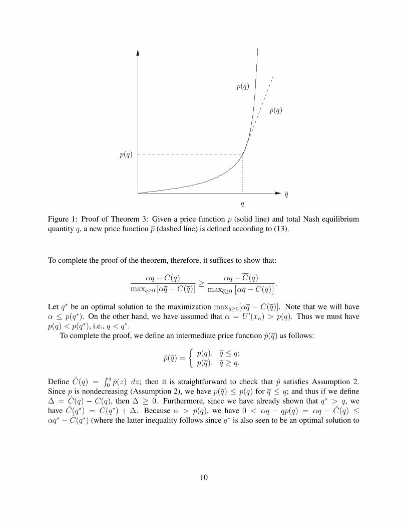
We now argue as follows. Define a new price function p(q) according to:

p(q) =

p(q), q ≤ q;

p(q) +(α − p(q))N

q(q − q), q ≥ q.

(13)

(See Figure 1 for an illustration.) Define C(q) =∫ q

0p(z) dz. Note that since α > p(q) and

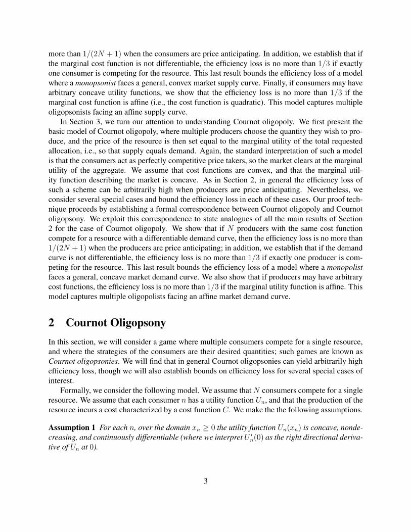
q > 0, p and C satisfy Assumption 2. It is also straightforward to check that the maximummaxq≥0[αq − C(q)] is achieved when p(q) = α, i.e., when q = q + q/N ; and furthermore, it isstraightforward to check that at this value of q we have αq −C(q) = (α− p(q))(q + q/(2N)). Onthe other hand, αq − C(q) = (α − p(q))q. Thus we have:

αq − C(q)

maxq≥0

[

αq − C(q)] =

2N

2N + 1.

9

PSfrag replacementsp(q)

q

p(q)

p(q)

q

Figure 1: Proof of Theorem 3: Given a price function p (solid line) and total Nash equilibriumquantity q, a new price function p (dashed line) is defined according to (13).

To complete the proof of the theorem, therefore, it suffices to show that:

αq − C(q)

maxq≥0 [αq − C(q)]≥

αq − C(q)

maxq≥0

[

αq − C(q)] .

Let q∗ be an optimal solution to the maximization maxq≥0[αq − C(q)]. Note that we will haveα ≤ p(q∗). On the other hand, we have assumed that α = U ′(xn) > p(q). Thus we must havep(q) < p(q∗), i.e., q < q∗.

To complete the proof, we define an intermediate price function p(q) as follows:

p(q) =

{

p(q), q ≤ q;p(q), q ≥ q.

Define C(q) =∫ q

0p(z) dz; then it is straightforward to check that p satisfies Assumption 2.

Since p is nondecreasing (Assumption 2), we have p(q) ≤ p(q) for q ≤ q; and thus if we define∆ = C(q) − C(q), then ∆ ≥ 0. Furthermore, since we have already shown that q∗ > q, wehave C(q∗) = C(q∗) + ∆. Because α > p(q), we have 0 < αq − qp(q) = αq − C(q) ≤αq∗ − C(q∗) (where the latter inequality follows since q∗ is also seen to be an optimal solution to

10

maxq≥0[αq − C(q)]). Thus we have:

αq − C(q)

αq∗ − C(q∗)≥

αq − C(q) − ∆

αq∗ − C(q∗) − ∆

=αq − C(q)

αq∗ − C(q∗). (14)

We now observe that C(q) = qp(q) = C(q), so the numerator in the last expression is αq− C(q) =αq − C(q). On the other hand, from (8) it follows that:

α = U ′( q

N

)

≤ p(q) +q

N·∂+p(q)

∂q. (15)

Rearranging, we conclude that:

∂+p(q)

∂q=

(α − p(q))N

q≤

∂+p(q)

∂q=

∂+p(q)

∂q. (16)

Thus since p is convex, we have p(q) ≥ p(q) for q ≥ q; on the other hand, we have p(q) = p(q)for q ≤ q. Since q∗ > q, we have C(q∗) ≥ C(q∗), so that αq∗ − C(q∗) ≤ αq∗ − C(q∗) ≤maxq≥0(αq − C(q)). Combining this inequality with (14) yields:

αq − C(q)

αq∗ − C(q∗)≥

αq − C(q)

maxq≥0

(

αq − C(q)) =

2N

2N + 1,

as required. 2

The preceding theorem can be used to yield bounds on efficiency loss in several special cases.We start with the following corollary, where all consumers share the same linear utility function.

Corollary 7 Suppose that N ≥ 1 consumers share the same linear utility function Un(xn) = αxn,where α > 0; in addition, suppose that Assumption 2 holds. If x

S is an optimal solution to (1)-(2),and x is a Nash equilibrium of the game defined by (Q1, . . . , QN), then:

∑

n

Un(xn) − C

(

∑

n

xn

)

≥

(

2N

2N + 1

)

(

∑

n

Un(xSn) − C

(

∑

n

xSn

))

. (17)

Proof. The proof follows the proof of Theorem 3, except that the Nash equilibrium may not beunique. The only step which requires modification is the derivation of (15)-(16), which relied onsymmetry of the Nash equilibrium.

We argue as follows. Let x be any Nash equilibrium, and let q =∑

n xn. By Lemma 5, we canagain assume without loss of generality that αq − C(q) > 0. This implies in turn that q > 0. Nowrecall the optimality condition (7) for each consumer n:

α ≤ p(q) + xn

∂+p(q)

∂q.

11

If we consider a consumer n such that xn ≤ q/N (at least one such consumer exists), then thepreceding inequality together with the fact that q > 0 implies:

(α − p(q))N

q≤

∂+p(q)

∂q.

This establishes (16), and the remainder of the proof of Theorem 3 follows. 2

Theorem 3 is useful in settings where uniqueness of the Nash equilibrium can be guaranteed.We now apply Theorem 3 in two special cases: first, a Cournot monopsony, where only one con-sumer is purchasing a scarce resource; and second, a Cournot oligopsony where all consumersshare the same utility function, and the price function is differentiable.

Corollary 8 Suppose that there is a single consumer (i.e., N = 1), with a utility function Usuch that Assumption 1 holds; in addition, suppose that Assumption 2 holds. Suppose also thatU(0) ≥ 0. If xS solves (1)-(2), and x maximizes U(x) − xp(x) over x ≥ 0, then:

U(x) − C(x) ≥

(

2

3

)

(

U(xS) − C(xS))

. (18)

This bound is tight, i.e., there exists a choice of U and C such that (18) holds with equality.

Proof. The proof relies on the following lemma.

Lemma 9 Suppose that there is a single consumer (i.e., N = 1), with a utility function U suchthat Assumption 1 holds; in addition, suppose that Assumption 2 holds. Then at least one ofthe following holds: either (1) all optimal solutions to maxx≥0[U(x) − xp(x)] are also optimalsolutions to (1)-(2); or (2) there exists a unique optimal solution to maxx≥0[U(x) − xp(x)].

Proof of Lemma. Suppose there exist x, x ∈ arg maxx≥0[U(x) − xp(x)] such that x 6= x.Assume without loss of generality that x < x; note that this implies x > 0. By concavity, wehave U ′(x) ≤ U(x). By (7), we have U ′(x) ≤ p(x) + x∂+p(x)/∂q. Since p is nondecreasing andconvex, and x < x, we have p(x) + x∂+p(x)/∂q ≤ p(x) + x∂−p(x)/∂q. Finally, from (8), wehave p(x) + x∂−p(x)/∂q ≤ U ′(x). Combining these inequalities, we have:

U ′(x) ≤ U(x) ≤ p(x) + x∂+p(x)

∂q≤ p(x) + x

∂−p(x)

∂q≤ U ′(x).

Thus equality must hold throughout; since x < x, this is only possible if p(x) = p(x) and∂+p(x)/∂x = ∂−p(x)/∂x = 0. Thus U ′(x) = p(x) and U ′(x) = p(x), so that both x and xare optimal solutions to (1)-(2), as required. 2

If all optimal solutions to maxx≥0[U(x) − xp(x)] are also optimal solutions to (1)-(2), thenthe bound (18) trivially holds. On the other hand, if there exists a unique optimal solution tomaxx≥0[U(x) − xp(x)], then we can apply Theorem 3 to conclude that (18) holds.

12

Finally, to see that the bound is tight, let U(x) = x, and let p(q) = (q − 1)+ (i.e., p(q) = 0 for0 ≤ q ≤ 1, and p(q) = q − 1 for q ≥ 1); thus C(q) = 0 if 0 ≤ q ≤ 1, and C(q) = (q − 1)2/2if q ≥ 1. Then it is straightforward to verify that x = 1 is the unique optimal solution tomaxx≥0[U(x) − xp(x)], while xS = 2 is an optimal solution to (1)-(2). Furthermore, we haveU(x) − C(x) = 1, while U(xS) − C(xS) = 3/2, matching the bound (18). 2

The preceding corollary considered a single consumer. We now consider a model consisting ofmultiple consumers who share the same utility function.

Corollary 10 Suppose that N ≥ 1 consumers share the same utility function Un = U , such thatAssumption 1 holds; in addition, suppose that Assumption 2 holds, and that p is differentiable.Suppose also that U(0) ≥ 0. If x

S is an optimal solution to (1)-(2), and x is a Nash equilibriumof the game defined by (Q1, . . . , QN), then:

∑

n

Un(xn) − C

(

∑

n

xn

)

≥

(

2N

2N + 1

)

(

∑

n

Un(xSn) − C

(

∑

n

xSn

))

. (19)

Proof. The proof relies on the following lemma.

Lemma 11 Suppose that Assumptions 1 and 2 hold, and that p is differentiable. Then at least oneof the following holds: either (1) all Nash equilibria of the game defined by (Q1, . . . , QN) are alsooptimal solutions to (1)-(2); or (2) there exists a unique Nash equilibrium of the game defined by(Q1, . . . , QN).

Proof of Lemma. The proof is similar to the proof of Lemma 9. Let x and x be two Nashequilibria such that x 6= x, and let q =

∑

n xn, and q =∑

n xn. Assume without loss of generalitythat q ≤ q. Since x 6= x, then there must exist a consumer n such that xn < xn; in particular, xn >0. In this case, we have U ′

n(xn) ≤ U ′n(xn) by concavity. By (7) we have U ′

n(xn) ≤ p(q) + xnp′(q).Since p is nondecreasing and convex, q ≤ q, and xn < xn, we have p(q)+xnp

′(q) ≤ p(q)+xnp′(q).

Since xn > 0, by (7)-(8) we have p(q) + xnp′(q) = U ′

n(xn). Combining these relations yields:

U ′n(xn) ≤ U ′

n(xn) ≤ p(q) + xnp′(q) ≤ p(q) + xnp′(q) = U ′

n(xn).

Thus equality must hold throughout; since xn < xn, this is only possible if p(q) = p(q), andp′(q) = p′(q) = 0. In this case (7)-(8) imply that for all m, we have U ′

m(xm) = p(q) if xm > 0,and U ′

m(xm) ≤ p(q) if xm = 0; similarly, U ′m(xm) = p(q) if xm > 0, and U ′

m(xm) ≤ p(q) ifxm = 0. These are precisely the optimality conditions for (1)-(2), so we conclude that both x andx are optimal solutions to (1)-(2), as required. 2

If all Nash equilibria are also optimal solutions to (1)-(2), then the bound (19) trivially holds.On the other hand, if there exists a unique Nash equilibrium, then we can apply Theorem 3 toconclude that (19) holds. 2

We note that Lemma 11 did not require all consumers to have the same utility function, andthus holds for any game where the price function p is differentiable. We also note that although

13

a tightness result is not claimed in the preceding corollary, such a result may be established byconsidering a limit of differentiable price functions which approach the worst case price functionp defined in the proof of Theorem 3. However, defining such price functions requires additionaltechnical complexity, and does not yield additional insight; thus the argument is omitted.

Note that Corollary 10 also yields a competitive limit theorem [17], since as N → ∞ theefficiency loss approaches zero. Indeed, this result is to be expected, since the consumers areassumed to be identical; thus in the limit of many consumers no single consumer should have asignificant impact on the market-clearing price.

Corollaries 7, 8, and 10 present bounds on efficiency loss under various restrictions on util-ity functions and the price function p. Although we have assumed differentiability of the utilityfunction, this assumption is not essential, as previously discussed; it only eases presentation ofthe technical arguments. By contrast, differentiability of the price function p is essential to theproof of Corollary 10. In particular, in considering the statements of Corollaries 7, 8, and 10, onemight expect a more general result to hold: if N consumers share the same utility function U andAssumption 1 is satisfied, and the price function p satisfies Assumption 2 (but is not necessarilydifferentiable), then the efficiency loss is no more than 1/(2N + 1) when consumers are priceanticipating. Such a result would be a generalization of Corollaries 7, 8, and 10.

However, the efficiency loss can be arbitrarily high if the price function is not differentiable,even if all consumers share the same utility function. The main reason for this negative result isthat when the price function is not differentiable, there may exist highly inefficient Nash equilibriawhich are not symmetric among the players. We present an example here of such a situation.

Example 2 Let the number of consumers be N > 1, and let the price function be p(q) = (q−1)+.Let C(q) =

∫ q

0p(z) dz be the associated cost function; note that p and C satisfy Assumption 2.

Define α = 1/N 2 and x = (α + 1)/N . We then define the piecewise linear utility function U asfollows:

U(x) =

{

αx, if x ≤ x;αx, if x ≥ x.

Then U is concave and continuous. Note that U is not differentiable, but as discussed above, thisfeature is inessential to the argument; a similar example can be constructed with a differentiableutility function U , at considerably higher technical expense.

We now claim that if xSn = x for all n, then x

S is a solution to (1)-(2). To see this, note thatqS =

∑

n xSn = Nx = α + 1; and thus p(qS) = α. On the other hand, we have:

∂+U(xSn)

∂xn

=∂+U(x)

∂x= 0 < α = p(qS);

∂−U(xSn)

∂xn

=∂−U(x)

∂x= α = p(qS).

These are necessary and sufficient optimality conditions for xS to be a solution to (1)-(2), as

required. Note that the aggregate surplus at this solution is∑

n U(xSn)−C(qS) = Nαx− α2/2 =

α2/2 + α.

14

Next, let xn = α for n = 2, . . . , N , and d1 = 1 − (N − 1)α. Note that q =∑

n xn = 1, andthus p(q) = 0 and:

∂−p(q)

∂q= 0;

∂+p(q)

∂q= 1.

We claim x is a Nash equilibrium; note that x is not symmetric among the players. Using thedefinitions of x and α, it is straightforward to establish that 0 < α < x < 1− (N − 1)α as long asN > 1. Thus, in particular, U is differentiable at xn for all n, and U ′(x1) = 0, while U ′(xn) = α.Now we observe that:

p(q) + x1

∂−p(q)

∂q= 0 = U ′(x1) < 1 − (N − 1)α = p(q) + x1

∂+p(q)

∂q;

p(q) + x1

∂−p(q)

∂q= 0 < U ′(xn) = α = p(q) + x1

∂+p(q)

∂q, n = 2, . . . , N.

Thus, the sufficient conditions (7)-(8) are satisfied, so we conclude x is a Nash equilibrium. Atthis Nash equilibrium, the aggregate surplus is

∑

n U(xn) − C(q) = αx + (N − 1)α2. If we nowsubstitute α = 1/N 2 and x = (α + 1)/N = 1/N 3 + 1/N , the ratio of Nash equilibrium aggregatesurplus to the maximal aggregate surplus reduces to:

1/N5 + 1/N 3 + (N − 1)/N 4

1/(2N 4) + 1/N 2.

As N → ∞, the preceding ratio approaches zero. 2

The preceding example highlights an important issue in market modeling: results on the perfor-mance of the market can be very sensitive under assumptions of symmetry among the participants.In particular, one might expect that little difference exists in market performance whether the pricefunction is differentiable or not; nevertheless, the preceding example shows that efficiency loss canbecome arbitrarily high if the price function is not differentiable.

To avoid such singular effects, we now search instead for a result that holds regardless of theutility functions of the consumers. Of course, such a result cannot hold for all price functions.In particular, we prove in the following theorem that if the price function is affine, the resultingefficiency loss is no more than 1/3 of the maximal aggregate surplus, regardless of the utilityfunctions of the consumers.

Theorem 12 Suppose that Assumption 1 holds, and that p(q) = aq + b for some a > 0, b ≥0. Suppose also that Un(0) ≥ 0 for all n. If x

S is any solution to (1)-(2), and x is any Nashequilibrium of the game defined by (Q1, . . . , QN ), then:

∑

n

Un(xn) − C

(

∑

n

xn

)

≥

(

2

3

)

(

∑

n

Un(xSn) − C

(

∑

n

xSn

))

. (20)

15

Furthermore, this bound is tight: for every a > 0, b ≥ 0, and δ > 0, there exists a choice of N anda choice of (linear) utility functions Un, n = 1, . . . , N , such that a Nash equilibrium x exists with:

∑

n

Un(xn) − C

(

∑

n

xn

)

≤

(

2

3+ δ

)

(

∑

n

Un(xSn) − C

(

∑

n

xSn

))

. (21)

Proof. The proof follows in two steps. Using Lemma 6, we first show that the worst case occurswhen the utility functions of the consumers are linear. We then optimize over all games with linearutility functions to determine the worst case efficiency loss.

Let x be a Nash equilibrium. As in the proof of Theorem 3, using Lemmas 4 and 5 wecan assume without loss of generality that

∑

n Un(xSn) − C(

∑

n xSn) > 0 and

∑

n U ′n(xn)xn −

C(∑

n xn) > 0. If we replace the utility function Un by Un for each n, where Un(xn) =(U ′

n(xn))xn, then x continues to be a Nash equilibrium, since the optimality conditions (7)-(8)still hold. Applying Lemma 6, therefore, we see that the ratio of Nash equilibrium aggregatesurplus to the maximal aggregate surplus can only be reduced if we replace Un by Un for all n.

Thus we assume without loss of generality that the utility functions of all consumers are linear,i.e., Un(xn) = αnxn. Since we have assumed

∑

n αnxn − C(∑

n xn) > 0, we know that αn > 0for at least one n. Thus, by replacing αn by αn/(maxm αm), and C(·) by C(·)/(maxn αn), we canalso assume without loss of generality that maxn αn = 1. Furthermore, by relabeling if necessary,we can assume that α1 = 1. Note that after rescaling, the new price function p is still affine butmay have a different slope.

Since we have restricted attention to settings where∑

n αnxn − C(∑

n xn) > 0, we must alsohave

∑

n xn > 0. Thus, from (8) and the fact that maxn αn = 1 we must have 1 > p(q) = aq + b;in particular, this implies that b < 1.

We start by computing the maximal aggregate surplus under these assumptions. Since the pricefunction is p(q) = aq + b, the maximal aggregate surplus is achieved when p(qS) = 1, i.e., whenqS = (1 − b)/a; this quantity is entirely allocated to consumer 1. The maximal aggregate surplusis thus:

1 − b

a−

(1 − b)2

2a−

b(1 − b)

a=

(1 − b)2

2a.

Since the maximal aggregate surplus is fixed as (1−b)2/(2a), by (7)-(8) the worst case game is

16

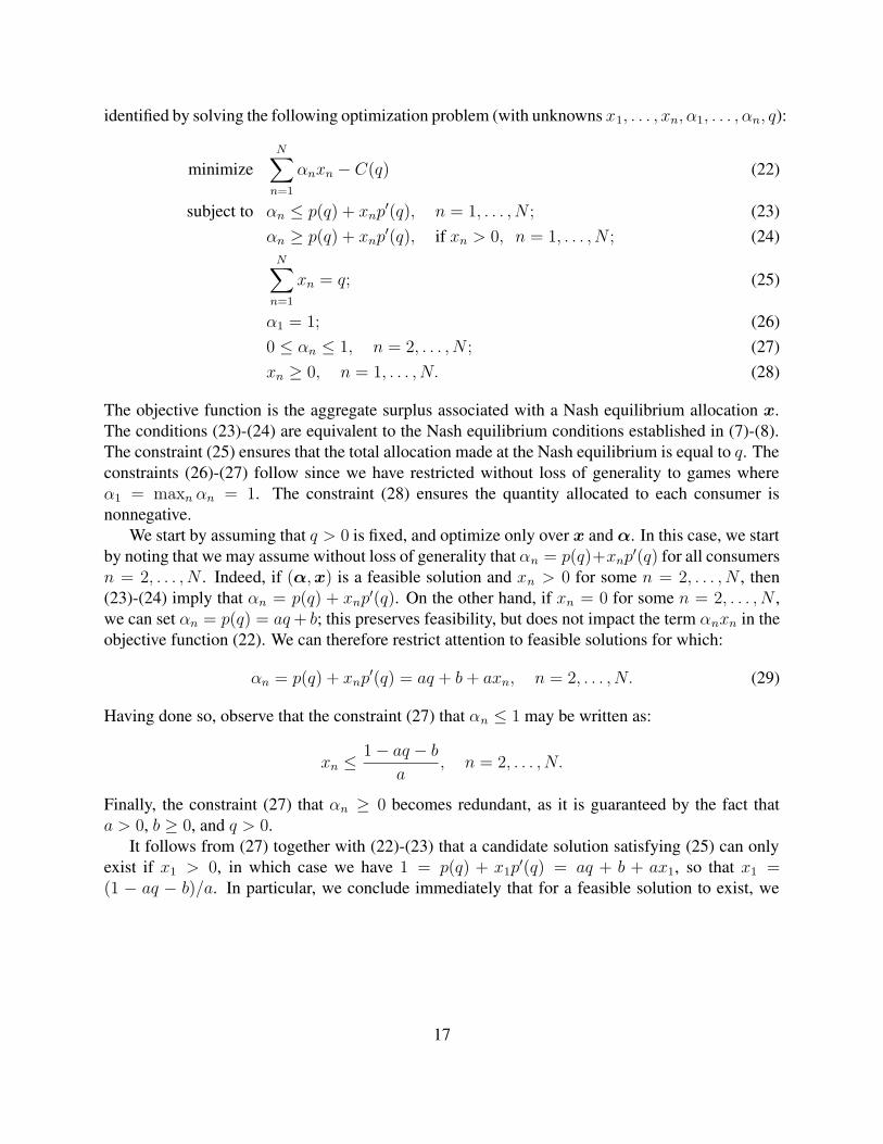
identified by solving the following optimization problem (with unknowns x1, . . . , xn, α1, . . . , αn, q):

minimizeN∑

n=1

αnxn − C(q) (22)

subject to αn ≤ p(q) + xnp′(q), n = 1, . . . , N ; (23)

αn ≥ p(q) + xnp′(q), if xn > 0, n = 1, . . . , N ; (24)

N∑

n=1

xn = q; (25)

α1 = 1; (26)0 ≤ αn ≤ 1, n = 2, . . . , N ; (27)xn ≥ 0, n = 1, . . . , N. (28)

The objective function is the aggregate surplus associated with a Nash equilibrium allocation x.The conditions (23)-(24) are equivalent to the Nash equilibrium conditions established in (7)-(8).The constraint (25) ensures that the total allocation made at the Nash equilibrium is equal to q. Theconstraints (26)-(27) follow since we have restricted without loss of generality to games whereα1 = maxn αn = 1. The constraint (28) ensures the quantity allocated to each consumer isnonnegative.

We start by assuming that q > 0 is fixed, and optimize only over x and α. In this case, we startby noting that we may assume without loss of generality that αn = p(q)+xnp

′(q) for all consumersn = 2, . . . , N . Indeed, if (α,x) is a feasible solution and xn > 0 for some n = 2, . . . , N , then(23)-(24) imply that αn = p(q) + xnp′(q). On the other hand, if xn = 0 for some n = 2, . . . , N ,we can set αn = p(q) = aq + b; this preserves feasibility, but does not impact the term αnxn in theobjective function (22). We can therefore restrict attention to feasible solutions for which:

αn = p(q) + xnp′(q) = aq + b + axn, n = 2, . . . , N. (29)

Having done so, observe that the constraint (27) that αn ≤ 1 may be written as:

xn ≤1 − aq − b

a, n = 2, . . . , N.

Finally, the constraint (27) that αn ≥ 0 becomes redundant, as it is guaranteed by the fact thata > 0, b ≥ 0, and q > 0.

It follows from (27) together with (22)-(23) that a candidate solution satisfying (25) can onlyexist if x1 > 0, in which case we have 1 = p(q) + x1p

′(q) = aq + b + ax1, so that x1 =(1 − aq − b)/a. In particular, we conclude immediately that for a feasible solution to exist, we

17

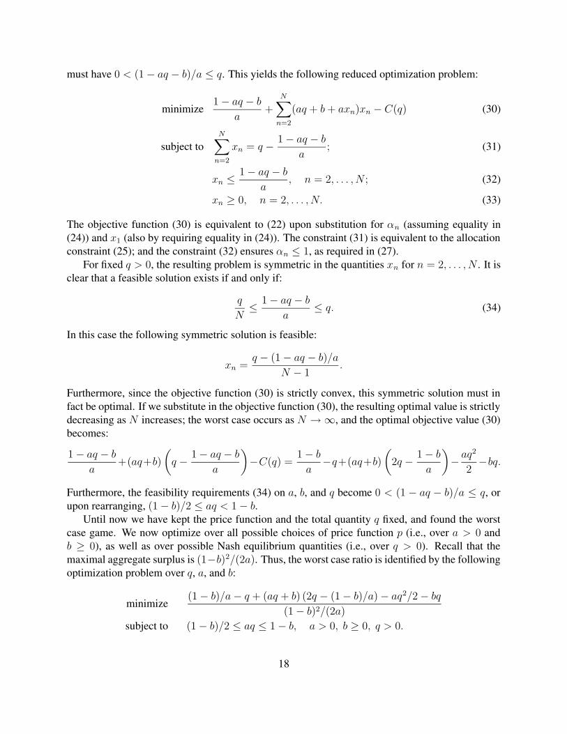
must have 0 < (1 − aq − b)/a ≤ q. This yields the following reduced optimization problem:

minimize1 − aq − b

a+

N∑

n=2

(aq + b + axn)xn − C(q) (30)

subject toN∑

n=2

xn = q −1 − aq − b

a; (31)

xn ≤1 − aq − b

a, n = 2, . . . , N ; (32)

xn ≥ 0, n = 2, . . . , N. (33)

The objective function (30) is equivalent to (22) upon substitution for αn (assuming equality in(24)) and x1 (also by requiring equality in (24)). The constraint (31) is equivalent to the allocationconstraint (25); and the constraint (32) ensures αn ≤ 1, as required in (27).

For fixed q > 0, the resulting problem is symmetric in the quantities xn for n = 2, . . . , N . It isclear that a feasible solution exists if and only if:

q

N≤

1 − aq − b

a≤ q. (34)

In this case the following symmetric solution is feasible:

xn =q − (1 − aq − b)/a

N − 1.

Furthermore, since the objective function (30) is strictly convex, this symmetric solution must infact be optimal. If we substitute in the objective function (30), the resulting optimal value is strictlydecreasing as N increases; the worst case occurs as N → ∞, and the optimal objective value (30)becomes:

1 − aq − b

a+(aq+b)

(

q −1 − aq − b

a

)

−C(q) =1 − b

a−q+(aq+b)

(

2q −1 − b

a

)

−aq2

2−bq.

Furthermore, the feasibility requirements (34) on a, b, and q become 0 < (1 − aq − b)/a ≤ q, orupon rearranging, (1 − b)/2 ≤ aq < 1 − b.

Until now we have kept the price function and the total quantity q fixed, and found the worstcase game. We now optimize over all possible choices of price function p (i.e., over a > 0 andb ≥ 0), as well as over possible Nash equilibrium quantities (i.e., over q > 0). Recall that themaximal aggregate surplus is (1−b)2/(2a). Thus, the worst case ratio is identified by the followingoptimization problem over q, a, and b:

minimize(1 − b)/a − q + (aq + b) (2q − (1 − b)/a) − aq2/2 − bq

(1 − b)2/(2a)

subject to (1 − b)/2 ≤ aq ≤ 1 − b, a > 0, b ≥ 0, q > 0.

18

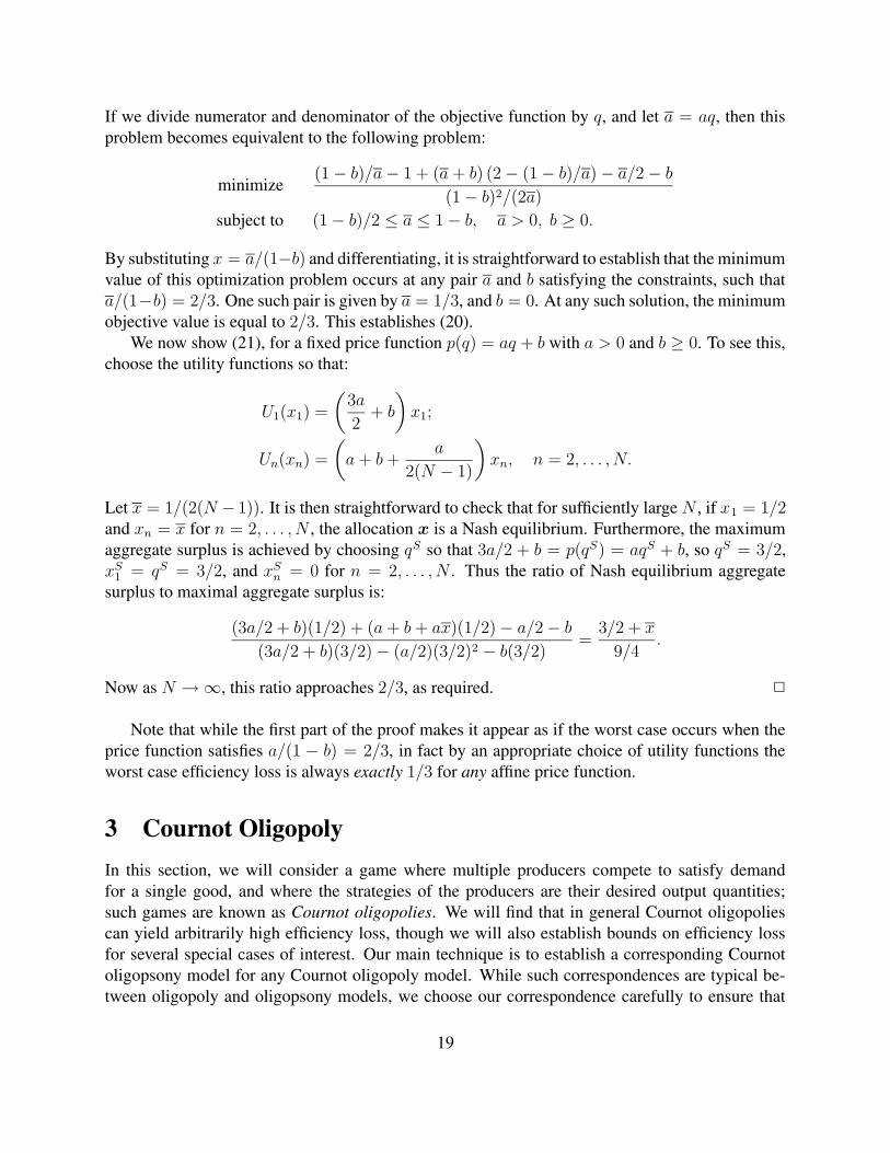
If we divide numerator and denominator of the objective function by q, and let a = aq, then thisproblem becomes equivalent to the following problem:

minimize(1 − b)/a − 1 + (a + b) (2 − (1 − b)/a) − a/2 − b

(1 − b)2/(2a)

subject to (1 − b)/2 ≤ a ≤ 1 − b, a > 0, b ≥ 0.

By substituting x = a/(1−b) and differentiating, it is straightforward to establish that the minimumvalue of this optimization problem occurs at any pair a and b satisfying the constraints, such thata/(1−b) = 2/3. One such pair is given by a = 1/3, and b = 0. At any such solution, the minimumobjective value is equal to 2/3. This establishes (20).

We now show (21), for a fixed price function p(q) = aq + b with a > 0 and b ≥ 0. To see this,choose the utility functions so that:

U1(x1) =

(

3a

2+ b

)

x1;

Un(xn) =

(

a + b +a

2(N − 1)

)

xn, n = 2, . . . , N.

Let x = 1/(2(N − 1)). It is then straightforward to check that for sufficiently large N , if x1 = 1/2and xn = x for n = 2, . . . , N , the allocation x is a Nash equilibrium. Furthermore, the maximumaggregate surplus is achieved by choosing qS so that 3a/2 + b = p(qS) = aqS + b, so qS = 3/2,xS

1 = qS = 3/2, and xSn = 0 for n = 2, . . . , N . Thus the ratio of Nash equilibrium aggregate

surplus to maximal aggregate surplus is:

(3a/2 + b)(1/2) + (a + b + ax)(1/2) − a/2 − b

(3a/2 + b)(3/2) − (a/2)(3/2)2 − b(3/2)=

3/2 + x

9/4.

Now as N → ∞, this ratio approaches 2/3, as required. 2

Note that while the first part of the proof makes it appear as if the worst case occurs when theprice function satisfies a/(1 − b) = 2/3, in fact by an appropriate choice of utility functions theworst case efficiency loss is always exactly 1/3 for any affine price function.

3 Cournot OligopolyIn this section, we will consider a game where multiple producers compete to satisfy demandfor a single good, and where the strategies of the producers are their desired output quantities;such games are known as Cournot oligopolies. We will find that in general Cournot oligopoliescan yield arbitrarily high efficiency loss, though we will also establish bounds on efficiency lossfor several special cases of interest. Our main technique is to establish a corresponding Cournotoligopsony model for any Cournot oligopoly model. While such correspondences are typical be-tween oligopoly and oligopsony models, we choose our correspondence carefully to ensure that

19

aggregate surplus values, efficient allocations, and Nash equilibria are unchanged between the twomodels; this allows derivation of efficiency loss results as simple analogues of all the main resultsof Section 2.

Formally, we consider the following model. We assume that N producers compete to satisfythe demand for a single good. We assume that each producer n has a cost function Cn whichgives the cost of production as a function of the amount produced. We also assume that producingq units of output yields an aggregate utility to the consumers of U(q). We make the followingassumptions.

Assumption 3 For each n, over the domain xn ≥ 0 the cost function Cn(xn) is convex, nonde-creasing, and continuously differentiable (where we interpret C ′

n(0) as the right directional deriva-tive of Cn at 0). In addition, Cn(0) = 0.

Assumption 4 There exists a continuous, nonincreasing function p(q) over q ≥ 0 such that forq ≥ 0:

U(q) =

∫ q

0

p(z)dz.

The function p(q) has the following properties:

1. p(0) > 0;

2. p(q) is concave with finite directional derivatives for q ≥ 0; and

3. p(q) → −∞ as q → ∞.

Thus U(q) is concave. We let qmax > 0 denote the unique quantity at which p(qmax) = 0.

We use U(q) to characterize the aggregate utility of the consumers. We restrict attention to thesetting where the marginal utility p(q) = U ′(q) (i.e., the inverse demand curve) is concave anddecreasing, from p(0) > 0 to p(qmax) = 0. In general in oligopoly models, the inverse demandcurve is either undefined for q ≥ qmax, or defined as p(q) = 0 for q ≥ qmax. These formulationshave the undesirable feature that the inverse demand curve p is not necessarily globally concaveafter such a transformation. For analytical simplicity, therefore, we have allowed p to becomenegative after qmax (cf. Condition 3 in Assumption 4). We make this assumption essentially withoutloss of generality: the revenue to producers would be zero at any aggregate production quantityq ≥ qmax, so that in considering either fully efficient production vectors or Nash equilibria it isstraightforward to check that we can restrict attention to vectors x such that

∑

n xn ≤ qmax. Inparticular, all the efficiency loss results of this section continue to hold for a model where we definep(q) = 0 for q ≥ qmax.

We note that Assumption 4 implies several basic facts about both p and U . Since p(0) > 0while p(qmax) = 0, p is strictly decreasing and negative for q ≥ qmax. Thus U(q) is strictlydecreasing for q > qmax.

We assume that both utility and cost are measured in monetary units, so that an efficient allo-cation is characterized by solving the following optimization problem:

20

maximize U

(

∑

n

xn

)

−∑

n

Cn(xn) (35)

subject to xn ≥ 0, n = 1, . . . , N. (36)

As before, the objective function (35) is the aggregate surplus. Since U(q) is strictly decreasingfor q > qmax and the objective function is continuous, it follows that an optimal solution exists; infact, we may conclude any optimal solution x

S satisfies∑

n xSn ≤ qmax.

We now consider the following pricing scheme. Each producer n chooses a desired outputquantity xn, and a single price µ(x) = p(

∑

n xn) is chosen. We first assume that given a priceµ > 0, producer n chooses xn to maximize:

Rn(xn; µ) = µxn − Cn(xn). (37)

Note that each producer acts as a price taker; since we are employing marginal utility pricing (i.e.,since µ(x) = p(

∑

n xn)), we again expect that price taking producers will maximize aggregatesurplus at a competitive equilibrium. This is formalized in the following proposition, a specialcase of the first fundamental theorem of welfare economics [17].

Proposition 13 Suppose Assumptions 3 and 4 hold. There exists a competitive equilibrium, thatis, a vector x and a scalar µ ≥ 0 such that µ = p(

∑

n xn), and:

Rn(xn; µ) = maxxn≥0

Rn(xn; µ), n = 1, . . . , N. (38)

Any such vector x solves (35)-(36). If the functions Cn are strictly convex, such a vector x isunique as well.

Proposition 13 shows that with marginal utility pricing, and if the producers behave as pricetakers, there exists a vector of quantities x where all producers have optimally chosen their xn,with respect to the given price µ = p(

∑

n xn); and at this “equilibrium,” the aggregate surplusis maximized. However, when the price taking assumption is violated, the model changes into agame and the guarantee of Proposition 13 is no longer valid.

Consider, then, an alternative model where the producers are price anticipating, rather thanprice taking, and play a Cournot game. We use the notation x−n to denote the vector of all quan-tities chosen by producers other than n; i.e., x−n = (x1, x2, . . . , xn−1, xn+1, . . . , xn). Then givenx−n, each producer n chooses xn ≥ 0 to maximize:

Tn(xn; x−n) = xnp

(

∑

m

xm

)

− Cn(xn). (39)

The payoff function Tn is similar to the payoff function Rn, except that the producer now antici-pates that the price will be set according to p(

∑

m xm). A Nash equilibrium of the game definedby (T1, . . . , TN ) is a vector x ≥ 0 such that for all n:

Tn(xn; x−n) ≥ Tn(xn; x−n), for all xn ≥ 0. (40)

21

It is straightforward to show that a Nash equilibrium exists for this game, using techniques sim-ilar to the proof of Proposition 2; see also [18] for more general conditions guaranteeing existenceof Nash equilibria.

Proposition 14 Suppose that Assumptions 3 and 4 hold. Then there exists a Nash equilibrium x

for the game defined by (T1, . . . , TN). Furthermore, any Nash equilibrium x satisfies∑

n xn ≤qmax.

Proof. The proof is nearly identical to the proof of Proposition 2, so we omit the details. Weonly check that

∑

n xn ≤ qmax for any Nash equilibrium x. If not, consider a producer n withxn > 0; the payoff Tn(xn; x−n) to this producer is negative. On the other hand, this producer canguarantee a payoff of zero by choosing xn = 0. Thus x could not have been a Nash equilibrium, acontradiction. 2

Since we have assumed p is concave and nonincreasing, it is straightforward to verify that thepayoff Tn of each producer n is concave in the strategy xn. Thus a vector x is a Nash equilibriumif and only if the following optimality conditions hold for each n, with q =

∑

n xn:

C ′n(xn) ≥ p(q) + xn

∂+p(q)

∂q; (41)

C ′n(xn) ≤ p(q) + xn

∂−p(q)

∂q, if xn > 0. (42)

We will now use these conditions to analyze the efficiency loss when producers are price anticipat-ing. We first show in the following example that, in general, the efficiency loss may be arbitrarilyhigh.

Example 3 Fix a > 1 and b > a − 1, and consider a price function p defined as follows:

p(q) =

{

a, 0 ≤ q ≤ 1;a − b(q − 1), q ≥ 1.

Thus qmax = 1 + a/b. Note that this yields:

U(q) =

aq, 0 ≤ q ≤ 1;

aq − 1

2b(q − 1)2, q ≥ 1.

We consider a game with N = 2 producers where C1(x1) = x1, and C2(x2) = ax2. In this case,since a > 1, note that aggregate surplus is maximized when p(q) = 1, i.e., when q = 1+(a−1)/b;and furthermore, this quantity should be produced entirely by producer 1. Thus the maximalaggregate surplus is U(q) − C1(q), or:

a

(

1 +a − 1

b

)

−1

2b

(

a − 1

b

)2

− 1 −a − 1

b= a − 1 +

(a − 1)2

2b. (43)

22

On the other hand, we claim that the vector x defined by:

x1 =a − 1

b;

x2 = 1 −a − 1

b,

is a Nash equilibrium. Observe that q = x1 +x2 = 1, so p(q) = a. Furthermore, ∂+p(q)/∂q = −b,∂−p(q)/∂q = 0. It then follows that (41)-(42) are satisfied by both producers 1 and 2. Since b > 0,these conditions are sufficient to ensure that x is a Nash equilibrium. Note that the aggregatesurplus at this Nash equilibrium is U(q) − C1(x1) − C2(x2), or:

a −a − 1

b− a

(

1 −a − 1

b

)

=(a − 1)2

b.

Comparing this expression with (43), it is clear that in the limit where b → ∞, the Nash equilibriumaggregate surplus approaches zero, and the maximal aggregate surplus approaches a − 1; thus theratio of Nash equilibrium aggregate surplus to the maximal aggregate surplus approaches zero. 2

As expected, the preceding example appears “symmetric” to Example 1. Indeed, we expect ageneral correspondence between a given model of oligopoly, and an appropriately defined modelof oligopsony. In the remainder of this section, we formally establish this correspondence; wethen exploit it to directly establish results on efficiency loss for Cournot oligopoly, from the re-sults already proven for Cournot oligopsony. Although such correspondences are common, thekey difficulty in the present development is that we must ensure aggregate surplus, efficient allo-cations, and Nash equilibria remain unchanged between an oligopoly model and its correspondingoligopsony model.

The following theorem is the main result in this development.

Theorem 15 Suppose that Assumptions 3 and 4 hold. Define the constant Γ ≥ 0 according to:

Γ = max {p(0), C ′1(qmax), . . . , C

′N(qmax)} . (44)

For each n, define:

U ′n(xn) =

{

Γ − C ′n(xn), if 0 ≤ xn ≤ qmax;

Γ − C ′n(qmax), if xn > qmax.

(45)

Define the associated utility function Un(xn) =∫ xn

0U ′

n(z)dz. In addition, define a new pricefunction p according to:

p(q) = Γ − p(q). (46)

Define an associated cost function C(q) =∫ q

0p(z) dz. Then:

1. Assumption 1 is satisfied by (U1, . . . , UN); and Assumption 2 is satisfied by p and C.

23

2. For any vector x ≥ 0 such that xn ≤ qmax for all n, there holds:

U

(

∑

n

xn

)

−∑

n

Cn(xn) =∑

n

Un(xn) − C

(

∑

n

xn

)

, (47)

as well as:

Tn(xn; x−n) = xnp

(

∑

m

xm

)

−Cn(xn) = Un(xn)−xnp

(

∑

m

xm

)

= Qn(xn; x−n). (48)

3. A vector xS solves (1)-(2) with utility functions U1, . . . , UN and cost function C if and only

if xS solves (35)-(36).

4. A vector x is a Nash equilibrium of the game defined by (T1, . . . , TN) if and only if x is aNash equilibrium of the game defined by (Q1, . . . , QN ) when the utility function of consumern is Un and the cost function is C.

Proof. We prove each of the four claims of the theorem in four separate steps.

Proof of Claim 1. Because Cn is continuously differentiable and convex for each n, we con-clude that U ′

n is continuous and nonincreasing for each n. Furthermore, by definition of Γ, we haveU ′

n(xn) ≥ 0 for all xn. Thus Assumption 1 is satisfied by (U1, . . . , UN).Next, observe that p(0) = Γ − p(0) ≥ 0; and since p(q) is continuous, concave, and nonin-

creasing, p(q) is continuous, convex, and nondecreasing. Finally, since p(q) → −∞ as q → ∞,we conclude p(q) → ∞ as q → ∞. Thus Assumption 2 is satisfied by p and C.

Proof of Claim 2. Suppose we are given a vector x such that xn ≤ qmax for all n. Let q =∑

n xn. We argue as follows:

U(q) =

∫ q

0

p(z) dz

= Γq −

∫ q

0

p(z) dz

= Γq − C(q).

Similarly, since xn ≤ qmax and Cn(0) = 0 for each n, we have:

Cn(xn) =

∫ xn

0

C ′n(z) dz

= Γxn −

∫ xn

0

U ′n(z) dz

= Γxn − Un(xn).

24

Finally, since p(q) = Γ − p(q), we have:

xnp(q) = Γxn − xnp(q).

Thus we have:U(q) −

∑

n

Cn(xn) =∑

n

Un(xn) − C(q),

as well as:xnp(q) − Cn(xn) = Un(xn) − xnp(q).

Proof of Claim 3. We already know that any optimal solution xS to (35)-(36) must satisfy

∑

n xn ≤ qmax. In light of (47), therefore, to establish Claim 3 it suffices to show the follow-ing: any solution x

S to (1)-(2) with utility functions U1, . . . , UN and cost function C satisfiesqS =

∑

n xSn ≤ qmax as well. Suppose not; then we have qS > qmax, so that p(q) < 0. But then

p(qS) > Γ, while U ′n(xS

n) ≤ Γ for all n. Thus for any user n with xSn > 0, we have U ′

n(xSn) < p(qS),

contradicting the optimality of xS . Thus we must have

∑

n xSn ≤ qS , and Claim 3 is established.

Proof of Claim 4. The proof is very similar to the proof of Claim 3. In light of (48), it sufficesto show that: (a) no producers would ever choose xn > qmax in the game defined by (T1, . . . , TN );and (b) no consumers would ever choose xn > qmax in the game defined by (Q1, . . . , QN). Theproof of (a) is similar to the argument given in the proof of Proposition 2: the payoff to a producern is always negative if xn > qmax, so such a choice is strictly dominated by xn = 0, which yieldspayoff zero. To prove (b), fix a strategy vector x, and let q =

∑

n xn. Note that U ′n(xn) ≤ Γ,

while if xn > qmax, then p(q) > Γ (since p(q) < 0). Thus, since Un is concave, nonnegative, andnondecreasing, we have Un(xn) ≤ U ′

n(xn)xn ≤ Γxn < p(q)xn. Thus the payoff to consumer n isnegative, while choosing xn = 0 yields a payoff to player n of zero. Thus any strategy xn > qmax

is strictly dominated by the choice xn = 0; so we conclude (b) holds as well. Combining (48) withclaims (a) and (b), Claim 4 is established. 2

Given an oligopoly model, the preceding theorem constructs an oligopsony model which sharesall the properties of the oligopoly model—in terms of aggregate surplus, efficient allocations, andNash equilibria. Using the preceding theorem, we can prove analogues of the main results ofSection 2 with little additional effort. We start with the following three results, which followdirectly from Corollaries 7, 8, and 10; and Theorem 15. Their proofs are therefore omitted.

Corollary 16 Suppose that N ≥ 1 producers share the same cost function Cn(xn) = αxn, whereα > 0; in addition, suppose that Assumption 4 holds. If x

S solves (35)-(36), and x is a Nashequilibrium of the game defined by (T1, . . . , TN), then:

U

(

∑

n

xn

)

−∑

n

Cn(xn) ≥

(

2N

2N + 1

)

(

U

(

∑

n

xSn

)

−∑

n

Cn(xSn)

)

. (49)

25

Corollary 17 Suppose that N = 1, and producer 1 has a cost function C such that Assumption3 holds; in addition, suppose that Assumption 4 holds. If xS solves (35)-(36), and x maximizesxp(x) − C(x) over x ≥ 0, then:

U(x) − C(x) ≥2

3

(

U(xS) − C(xS))

. (50)

Corollary 18 Suppose that N ≥ 1 producers share the same cost function Cn = C, such thatAssumption 3 holds; in addition, suppose that Assumption 4 holds, and that p is differentiable inthe region (0, qmax). If x

S solves (35)-(36), and x is a Nash equilibrium of the game defined by(T1, . . . , TN), then:

U

(

∑

n

xn

)

−∑

n

Cn(xn) ≥

(

2N

2N + 1

)

(

U

(

∑

n

xSn

)

−∑

n

Cn(xSn)

)

. (51)

Corollary 16 is closely related to the results of Anderson and Renault [1]. Specifically, byusing equation (12) of [1], it is possible to show that the aggregate surplus at a Nash equilibriumis no worse than a factor 2N/(N + 1)2 of the maximal aggregate surplus, when N firms share thesame linear cost function, and demand satisfies Assumption 4. However, the bound in [1] allowsthe efficiency loss to approach 100% as N → ∞, whereas the result of Corollary 16 shows thatefficiency loss approaches zero as N → ∞ (a competitive limit, as expected).

Note also that Corollary 17 establishes an efficiency loss result for the classical monopolymodel [24]. The efficiency loss is no worse than 33%, allowing for both a general convex producercost function and general concave demand.

The next result is an analogue of Theorem 12.

Theorem 19 Suppose that Assumption 4 holds, and that p(q) = b − aq for some a > 0, b > 0. Ifx

S is any solution to (35)-(36), and x is any Nash equilibrium of the game defined by (T1, . . . , TN),then:

U

(

∑

n

xn

)

−∑

n

Cn(xn) ≥2

3

(

U

(

∑

n

xSn

)

−∑

n

Cn(xSn)

)

. (52)

Furthermore, this bound is tight: for every a > 0, b > 0, and δ > 0, there exists a choice of N anda choice of (linear) cost functions Cn, n = 1, . . . , N , such that a Nash equilibrium x exists with:

∑

n

Un(xn) − C

(

∑

n

xn

)

≤

(

2

3+ δ

)

(

∑

n

Un(xSn) − C

(

∑

n

xSn

))

. (53)

Proof. Note that if p is affine with negative slope and positive intercept, then p as defined in(46) is also affine with positive slope and intercept; thus (52) follows by Theorems 12 and 15.

To establish (53), fix a price function p(q) = b − aq with a, b > 0, and define Cn as follows:

C1(x1) = 0;

Cn(xn) =

(

b

3

)(

N − 2

N − 1

)

xn, n = 2, . . . , N.

26

Let x = b/(3a(N−1)). It is then straightforward to check that for sufficiently large N , if x1 = b/3aand xn = x for n = 2, . . . , N , the allocation x is a Nash equilibrium; to see this, simply note that(42) holds with equality for all n. At this Nash equilibrium, the resulting aggregate surplus is givenby:

4b2

9a−

b2

9a·N − 2

N − 1.

Furthermore, the maximum aggregate surplus is achieved by choosing qS so that p(qS) = 0, soqS = b/a, xS

1 = qS = b/a, and xSn = 0 for n = 2, . . . , N . This yields maximal aggregate surplus

b2/(2a). Thus as N → ∞, the ratio of Nash equilibrium aggregate surplus to maximal aggregatesurplus approaches 2/3, as required. 2

Finally, as in Example 2, there exist oligopoly models where all producers share an identicalcost function, and the price function p is not differentiable, for which the efficiency loss can bearbitrarily high at a Nash equilibrium. For completeness we present such an example.

Example 4 Let the number of producers be N > 1. We build an example which is analogous toExample 2. Define α = 1/N 2 and x = (α + 1)/N . Let the price function p be given by:

p(q) =

{

α, if q ≤ 1;α − (q − 1), if q ≥ 1.

Note that with this definition we have qmax = α + 1. Define a single cost function C(x) byC(x) = α(x − x)+. We assume all producers share the same cost function C.

It is now straightforward to establish that under the transformation described in Theorem 15,we have Γ = α and we recover exactly the model described in Example 2. It thus follows that asN → ∞, the efficiency loss can be arbitrarily high when producers are price anticipating. 2

4 ConclusionThis paper has considered models of both Cournot oligopsony and Cournot oligopoly, and estab-lished bounds on efficiency loss in both cases—i.e., bounds on the ratio of aggregate surplus at aNash equilibrium to the maximum possible aggregate surplus. We find that while efficiency loss isgenerally arbitrarily high, in several special cases of interest the efficiency loss may be bounded.The most interesting results are those which hold independent of the characteristics of the marketparticipants, Theorem 12 and Corollary 19. These results show that for general concave consumerutility functions with affine market supply (for Cournot oligopsony), or for general convex pro-ducer cost functions with affine market demand (for Cournot oligopoly), the efficiency loss is noworse than 1/3 of the maximal aggregate surplus.

AcknowledgmentThis work was partially supported by the National Science Foundation under a Graduate ResearchFellowship and grant ECS-0312921.

27

References[1] S. P. Anderson and R. Renault. Efficiency and surplus bounds in Cournot competition. Jour-

nal of Economic Theory, 113:253–264, 2003.

[2] E. Anshelevich, A. Dasgupta, E. Tardos, and T. Wexler. Near-optimal network design withselfish agents. In Proceedings of the 35th Annual ACM Symposium on the Theory of Com-puting, pages 511–520, 2003.

[3] A. Bergson. On monopoly welfare losses. American Economic Review, 63(5):853–870, 1973.

[4] J. R. Correa, A. S. Schulz, and N. Stier Moses. Selfish routing in capacitated networks.Mathematics of Operations Research, 2004. To appear.

[5] A. A. Cournot. Recherches sur les Principes Mathematiques de la Theorie des Richesses.Macmillan and Co., New York, New York, 1897. Translated by N.T. Bacon; originally pub-lished in 1838.

[6] R. E. Dansby and R. D. Willig. Industry performance gradient indexes. The American Eco-nomic Review, 69(3):249–260, 1979.

[7] A. F. Daughety, editor. Cournot Oligopoly. Cambridge University Press, Cambridge, UnitedKingdom, 1988.

[8] N. R. Devanur, N. Garg, R. Khandekar, V. Pandit, A. Saberi, and V. V. Vazirani. Price ofanarchy, locality gap, and a network service provider game. 2004. In preparation.

[9] A. Fabrikant, A. Luthra, E. Maneva, C. Papadimitriou, and S. Shenker. On a network creationgame. In Proceedings of the 22nd Annual ACM Symposium on Principles of DistributedComputing, pages 347–351, 2003.

[10] J. W. Friedman. Oligopoly and the Theory of Games. North-Holland Publishing Company,Amsterdam, The Netherlands, 1977.

[11] A. C. Harberger. Monopoly and resource allocation. American Economic Review, 44(2):77–87, 1954.

[12] A. Haurie and P. Marcotte. On the relationship between Nash-Cournot and Wardrop equilib-ria. Networks, 15(1):295–308, 1985.

[13] R. Johari, S. Mannor, and J. N. Tsitsiklis. Efficiency loss in a network resource allocationgame: the case of elastic supply. Publication 2605, MIT Laboratory for Information andDecision Systems, 2004.

[14] R. Johari and J. N. Tsitsiklis. Efficiency loss in a network resource allocation game. Mathe-matics of Operations Research, 29(3):407–435, 2004.

28

[15] E. Koutsoupias and C. Papadimitriou. Worst-case equilibria. In Proceedings of the 16thAnnual Symposium on Theoretical Aspects of Computer Science, pages 404–413, 1999.

[16] A. Manning. Monopsony in Motion: Imperfect Competition in Labor Markets. PrincetonUniversity Press, Princeton, New Jersey, 2003.

[17] A. Mas-Colell, M. D. Whinston, and J. R. Green. Microeconomic Theory. Oxford UniversityPress, Oxford, United Kingdom, 1995.

[18] W. Novshek. On the existence of Cournot equilibrium. Review of Economic Studies,52(1):85–98, 1985.

[19] W. Novshek and H. Sonnenschein. Cournot and Walras equilibrium. Journal of EconomicTheory, 19(2):223–266, 1978.

[20] J. Rosen. Existence and uniqueness of equilibrium points for concave n-person games.Econometrica, 33(3):520–534, 1965.

[21] T. Roughgarden and E. Tardos. How bad is selfish routing? Journal of the ACM, 49(2):236–259, 2002.

[22] R. Ruffin. Cournot oligopoly and competitive behavior. Review of Economic Studies,38(4):493–502, 1971.

[23] C. Shapiro. Theories of oligopoly behavior. In R. Schmalensee and R. D. Willig, editors,Handbook of Industrial Organization, volume 1, pages 329–414. Elsevier Science, Amster-dam, The Netherlands, 1989.

[24] J. Tirole. The Theory of Industrial Organization. MIT Press, Cambridge, Massachusetts,1988.

29