EEG Artifact Detection - pdfs.semanticscholar.org · 7 | Page 3.1 Applications The EEG is indicated...

EEG

Artifact

Detection

Iván Manuel Benito Núñez

Department of Cybernetics

Czech Technical University in Prague

Prague June 2010

2 | P a g e

Contents

1 Introduction .............................................................................................................. 3

2 Brain .......................................................................................................................... 3

2.1 Cerebral cortex lobes ......................................................................................... 4

3 Electroencephalography ........................................................................................... 5

3.1 Applications ....................................................................................................... 7

3.1.1 Epilepsy ....................................................................................................... 7

3.1.2 Sleep ........................................................................................................... 8

3.1.3 Sleep states ................................................................................................. 8

3.1.4 Dementia .................................................................................................. 10

3.2 Important frequency bands ............................................................................. 10

3.2.1 Delta.......................................................................................................... 10

3.2.2 Theta ......................................................................................................... 11

3.2.3 Alfa ............................................................................................................ 11

3.2.4 Beta ........................................................................................................... 11

3.3 Artifacts ............................................................................................................ 11

3.3.1 Power line artefact ................................................................................... 12

3.3.2 Muscle artifact .......................................................................................... 12

3.3.3 Eye blinks .................................................................................................. 12

3.3.4 Eye movement .......................................................................................... 13

3.3.5 Sweat artifact ............................................................................................ 13

4 Signal processing .................................................................................................... 13

4.1 Segmentation ................................................................................................... 13

4.2 Feature extraction ........................................................................................... 13

4.3 Example of signal analysis using Matlab .......................................................... 14

4.4 Methods for Classification ............................................................................... 18

4.4.1 Knn algorithm ........................................................................................... 19

5 Artefact detection program in C++ ......................................................................... 19

5.1 How to use the program .................................................................................. 20

5.1.1 Command-line mode ................................................................................ 20

5.1.2 Interactive mode ...................................................................................... 22

5.1.3 Program results ........................................................................................ 23

5.2 Explaining the implementation ........................................................................ 25

5.3 Structure of data files ...................................................................................... 26

5.3.1 Standard and Extended header ................................................................ 27

5.3.2 Tag tables .................................................................................................. 27

5.4 Adapt/extend the project ................................................................................ 28

5.5 Project Settings in Windows ............................................................................ 29

6 Conclusions ............................................................................................................. 32

7 Bibliography ............................................................................................................ 33

3 | P a g e

1 Introduction

This report presents an overview in the area of electroencephalography (EEG) with

special emphasis on pattern recognition techniques. In the first steps, basics about the

human brain are explained, some important applications of electroencephalography

are described and the relevant signals and artifacts are introduced. After the

introduction, it is given an explanation of the steps that were followed to implement a

program in Matlab that finds the most relevant characteristics of the EEG data which is

useful to achieve a good pattern classification. Finally the implementation of a more

complex program in C++ is described with the aim of putting in use a pattern

recognition methodology in order to find parts of EEG signals affected by artifacts.

Artifacts increase the difficulty of analysing EEG in that way that recordings can be

unreadable or artifacts can be misinterpreted as pathological activity. Recognition and

elimination of artifacts is a complicated task, usually performed by a human expert.

Disadvantage of this approach is that elimination of artifacts means discarding possibly

a large amount of data, which can greatly decrease the amount of data available for

analysis.

The pattern recognition techniques involve the automatic classification of data. These

techniques are applied for example in speech recognition, classification of text into

several categories, automatic recognition of images of human faces and finding more

and more applications each day. By taking an electroencephalogram, the amount of

information obtained can be too high in time and space. Some tests, such as those

related to sleep, may last longer than 8 hours. Pattern recognition techniques applied

to EEG are able to reduce the work to be done by the specialist, allowing them to focus

on the most relevant aspects.

At present, there are many studies that have developed highly efficient solutions in the

encephalogram data analysis. Besides, each day more complex and efficient

techniques appear, it is a branch of research in constant development. This project has

not attempted to develop a method of pattern recognition that provides classifications

with best results and minimum error rates. However, the main motivation was to

know in depth the methodology applied in pattern recognition, acquire skills to work

and discover new methods of classification.

2 Brain

The brain is an extremely complex organ of the nervous system rich in neurons with

specialized functions and interconnected via long protoplasmic fibres called axons and

dendrites. The outermost layer of the brain is the cerebral cortex, with 2 to 4 mm

thick, contains roughly 15–33 billion neurons and plays a key role in memory,

attention, perceptual awareness, thought, language, and consciousness [1].

The transmission of information within the brain is produced by substances called

neurotransmitters, substances that

These neurotransmitters are received by

The brain uses biochemical energy from cell metabolism as a trigger of neuronal

responses.

2.1 Cerebral cortex l

A lobe is a part of the cerebral cortex that subdivides the brain depending in its

function.

There are four main lobes (

� Frontal lobes: The frontal lobes are considered our emotional control

and home to our personality

attention, long-term memory

� Parietal lobes: They are connected with the processing of nerve impulses

related to the senses, such as touch, pain, taste, pressure, and temperature.

They also have language functions.

� Occipital lobes: The occipital lobe is involv

recognize objects. It is responsible for our vision.

� Temporal lobes: The temporal lobes are involved in the primary organization of

sensory input [2]. Individuals with

words or pictures into categories.

Figure


neurotransmitters, substances that are capable of causing nerve impulse transmission.

These neurotransmitters are received by the dendrites and are emitted


Cerebral cortex lobes

a part of the cerebral cortex that subdivides the brain depending in its

(Figure 1):

The frontal lobes are considered our emotional control

and home to our personality, controls voluntary movements, the capacity of

term memory and planning, among other things

They are connected with the processing of nerve impulses


They also have language functions.

The occipital lobe is involved with the brain's ability to

recognize objects. It is responsible for our vision.

The temporal lobes are involved in the primary organization of

. Individuals with temporal lobes lesions have difficulty placing

words or pictures into categories.

Figure 1: Human skull (brain lobes positions)

4 | P a g e


of causing nerve impulse transmission.

the dendrites and are emitted by axons.


a part of the cerebral cortex that subdivides the brain depending in its

The frontal lobes are considered our emotional control centre

, the capacity of

among other things.

They are connected with the processing of nerve impulses


ed with the brain's ability to

The temporal lobes are involved in the primary organization of

temporal lobes lesions have difficulty placing

5 | P a g e

3 Electroencephalography

An electroencephalogram (EEG) is a test that measures and records the electrical

activity of the brain. The common method to perform the test is placing electrodes

along the scalp that will transmit the obtained information to a recorder machine. The

amplitude of the EEG is about 100 µV when measured on the scalp, and about 1-2 mV

when measured on the surface of the brain. The clinical relevant bandwidth of this

signal is from under 1 Hz to about 50 Hz [3].

With this method is possible to determine the activity on a specific location within the

brain and to evaluate brain disorders, is the most common reason to diagnose and

monitor seizure disorders.

EEGs can also help to identify causes of other problems such as sleep disorders and

changes in behaviour. EEGs are sometimes used to evaluate brain activity after a

severe head injury or before heart or liver transplantation.

The patient has to be educated to behaviour during the process. Lying on a bed or sit

in a chair, he has to be relaxed and maybe he will be ask to close the eyes and be still

during the examination. Depending on the test is possible to use a light in some part of

the study or to breathe quickly [4].

Levels of arousal, sleeping, relaxing and action, all have a characteristic brainwave

pattern.

The activity of the brain is determined in microvolt (µV), and it has to be amplified in a

1.000.000 factor to be showed in a computer screen.

Electrodes

The electrodes are simply small metallic disc devices that provide the conduction of

potential electrocortical by wires towards the amplification device and a recording

machine. They can be made of gold, silver, tin or copper and are glued to the scalp

using a special conductive paste.

To help in the placement of the electrodes there are a special flexible head cover

called electrode cap. A disadvantage which has characterized these caps is indicated to

be the fact that the electrode positions are fixed, and are not individually adjustable

for the requirements peculiar to each individual electrographic analysis and patient [5].

With the right size and requirements of the electrode cap the time of placement and

consequently the comfort for the patient are improved.

Placement of electrodes

The placement of the electrodes is commonly standardized to be able to perform an

analysis of the given information in any laboratories. The most typical model is called

“10-20 International System of Electrode Placement” (¡Error! No se encuentra el

origen de la referencia.). In this system 21 electrodes are located on the surface of the

scalp. The "10" and "20" refer to the fact that the actual distances between adjacent

6 | P a g e

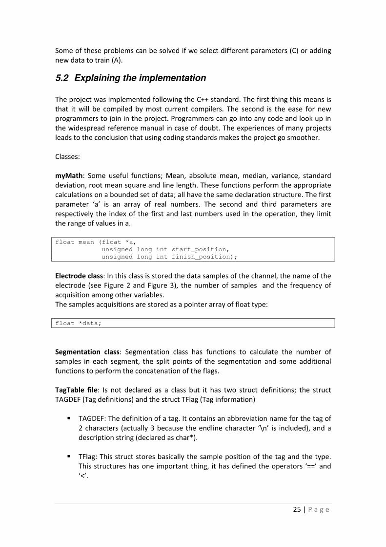
electrodes are either 10% or 20% of the total front-back or right-left distance of the

skull . Often the earlobe electrodes called A1 and A2, connected respectively to the left

and right earlobes, are used as the reference electrodes.

In addition to the 21 electrodes of the international 10-20 system, intermediate 10%

electrode positions are also used. The locations and nomenclature of these electrodes

are standardized by the American Electroencephalographic Society. In this

recommendation, four electrodes have different names compared to the 10-20

system; these are T7, T8, P7, and P8. These electrodes are drawn grey in the ¡Error! No

se encuentra el origen de la referencia..

Pz

Cz

Fz

C3

T3

A1 C4 T4 A2

F7

Fp1

F3

Fp2

F8

F4

P4

T6

T5

P3

O1 O2

The letters used are:

F Frontal lobe

T Temporal lobe

C Central lobe

P Parietal lobe

O Occipital lobe

Figure 2. 10-20 International System of Electrode Placement

7 | P a g e

3.1 Applications

The EEG is indicated in all paroxysmal phenomenons in which the cause is suspected to

be of cerebral origin and in all situations of brain dysfunction, especially in

symptomatic phase. For example in epilepsy, encephalopathy, coma, diagnosis of brain

death, brain tumours and other space-occupying lesions, dementia, degenerative

diseases to the nervous system, cerebrovascular disease, head injury, headache,

vertigo and psychiatric disorders.

Is the most common and most useful test performed in evaluating patients suspected

of epilepsy.

3.1.1 Epilepsy

Epilepsy is a brain disorder that causes people to have recurring seizures. A seizure is

usually defined as a sudden alteration of behaviour due to a temporary change in the

electrical functioning of the brain, in particular the outside rim of the brain called the

cortex [6]. It is usually diagnosed after a person has had at least two seizures that were

not caused by some known medical condition like alcohol withdrawal or extremely low

blood sugar. An epileptic attack may result in a series of involuntary contractions of

Iz

Oz

POz

Pz

CPz

Cz

FCz

Fz

AFz

FPZ

C1 C3 C5 T7 T9 C2 C4 C6 T8 T10

FC1 FC2 FC3

FC5 FT7

F7

Fp1

AF7

F1 F3 F5

AF3

Fp2

AF8

F8

FT8

FC4 FC6

F2 F4 F6

AF4

CP2

CP4

CP6

TP8

CP1 CP3 CP5

TP7

P2 P4

P8 P6

P1 P7

P5 P3

O1

PO7

O2

PO8

PO4 PO3

Figure 3. Location and nomenclature of the intermediate 10% electrodes, as standardized by the American

Electroencephalographic Society

8 | P a g e

the voluntary muscles, abnormal sensations, abnormal behaviours, or some

combination of these events.

Epilepsy has many possible causes, including illness, brain injury and abnormal brain

development. In many cases, the cause is unknown.

There is no cure for epilepsy, but medicines can control seizures for most people.

When medicines are not working well, surgery or implanted devices such as vagus

nerve stimulators may help. Special diets can help some children with epilepsy [7].

3.1.2 Sleep

Sleep is a physical and mental resting state in which a person becomes relatively

inactive and unaware of the environment. In essence, sleep is a partial detachment

from the world, where most external stimuli are blocked from the senses [8].

The brain repeats a cycle along the normal sleep that lasts about 90-120 minutes and is

repeated four or five times each night. In this cycle is differentiated by dramatically

different forms of brain activity the different stages.

3.1.3 Sleep states

We can divide the normal sleep in two main types, the REM (Rapid eye movement)

which involves intense brain self-activation and NREM (non-rapid eye movement)

states. NREM sleep is subdivided into 4 substates.

70-80% of the time during a night the brain is in NREM sleep and the other time in

REM.

Most dreaming takes place during REM sleep. At least in mammals, a descending

muscular atonia is seen in this state, the brain blocks signals to the muscles to remain

immobile so dreams will not be acted out.

Awake

Stage 1

Stage 2

Stage 3

Stage 4

REM

REM

REM

REM

REM

Hour 1 Hour 2 Hour 3 Hour 4 Hour 5 Hour 6 Hour 7 Hour 8

Figure 4. Sleep states of an adult during the night

9 | P a g e

Table 1 shows some basics discriminations factors about sleep states.

EEG characteristic Time in this

stage

Eye activity

N

R

E

M

Stage 1 Activity generally in theta

range.

10-12 min. Slow eye

movements

Stage 2 • Sleep spindles (12-14 hz

waveforms) of at least 0.5

seg.

• K-Complexes (a negative

wave followed by a

positive one)

• Appear delta

waveforms.

40-55% of

total sleep

time.

No

detected.

Stage 3 Slow-

wave

sleep.

Moderate

amount of

high-

amplitude.

14-15 % of

total sleep

time.

Stage 4

Large

amounts of

high-

amplitude.

R

E

M

Tonic As awake. 20-25 % of

total sleep

time.

Rapid eye

movement

Phasic

Table 1. Basic sleep states information

Table 2 shows that children need more sleep per day in order to develop and function

properly: up to 18 hours for newborn babies, with a declining rate as a child ages. A

newborn baby spends almost 9 hours a day in REM sleep. By the age of five or so, only

slightly over two hours is spent in REM.

Average Hours of Sleep Per Day

Newborn 18

1 month 15–16

6 months 14–15

1 year 13–14

2 years 13

3 years 12

5-6 years 11

7-8 years 10

9–17 years 9–11

Adults, Including elderly 7–8 Table 2. Hours of sleep by age

3.1.4 Dementia

Dementia is not a specific disease. It is a descriptive term for a collection of symptoms

that can be caused by a number of disorders that affect the

dementia have significantly impaired intellectual functioning that interferes with

normal activities and relationships

the brain that is affected. One of the main classifications divides dementias into two

main groups: cortical and sub

degeneration occurs [10]. The most important cortical deme

(AD), which accounts for approximately 50% of the cases. Other known cortical

abnormalities are Pick’s disease and Creutzfeldt

hand, the most common subcortical diseases are Parkinson’s disease

disease, lacunar state, normal pressure hydrocephalus, and progressive supranuclear

palsy [11].

3.2 Important frequency bands

The classification of EEG waveform

amplitude and shape. The

relevant.

Actually the frequency of brain waves

but not this entire spectrum is going to be considered

is divided in four main group

(alpha, beta, theta and delta

The most popular way to apply a frequency analysis

Fast Fourier Transform algorithm.

3.2.1 Delta

High amplitude brain waves

in deep sleep in adults as well as in infants and children.

As they are rarely in awake experie

indicator of a brain lesion.

Figure 5. Example of an EEG


that can be caused by a number of disorders that affect the brain. People with


al activities and relationships [9]. Dementias are often classified by the region of

affected. One of the main classifications divides dementias into two

main groups: cortical and sub-cortical based on the area of the brain where

The most important cortical dementia is Alzheimer’s disease


abnormalities are Pick’s disease and Creutzfeldt–Jakob diseases (CJD).

hand, the most common subcortical diseases are Parkinson’s disease


Important frequency bands

waveforms are commonly made according to their frequency,

he site on the scalp from where the data is recorded is

he frequency of brain waves range can be recognize from 0.5 to 500 Hz

spectrum is going to be considered important in the

groups of frequency ranges that are more clinically relevant

alpha, beta, theta and delta waves).

The most popular way to apply a frequency analysis is on a digital computer using the

Fast Fourier Transform algorithm.

High amplitude brain waves which have a frequency of 3 Hz or less, are normally seen

deep sleep in adults as well as in infants and children.

As they are rarely in awake experience in adults the existence of delta wave can be an

Example of an EEG delta wave, one second sample

10 | P a g e


brain. People with


Dementias are often classified by the region of

affected. One of the main classifications divides dementias into two

cortical based on the area of the brain where

ntia is Alzheimer’s disease


Jakob diseases (CJD). On the other

hand, the most common subcortical diseases are Parkinson’s disease, Huntington’s


o their frequency,

site on the scalp from where the data is recorded is also

0.5 to 500 Hz [12],

the examination; it

ranges that are more clinically relevant

is on a digital computer using the

are normally seen

of delta wave can be an

3.2.2 Theta

Theta waves lie within the range of

and REM state. The theta wave plays an important role in infancy and childhood.

Larger contingents of theta wave activity in the waking adult are abnormal and are

caused by various pathological problems

Theta waves are generated from the interaction between temporal and frontal lobe.

3.2.3 Alfa

For Alfa waves the frequency is in the range of 8 and 12

relax states. This kind of wave appears

Predominantly they are originated in the occipital lobe during relaxing periods,

the eyes, but awake. They are a

3.2.4 Beta

For Beta waves the frequency is in the range of

the person is awake and with

Parkinson’s disease and this links to

3.3 Artifacts

Signals that are detected by an EEG but not belong

artifacts. They may occur at many points during the recording process.

of artifacts can be quite large relative to the size of amplitude of the cortical signals of

interest. The range of physiological and nonphysiological artifacts is very wide.

of common artifacts include:

respiratory artifact, electrode popping, ECG artifact, sweat artifact, loose/broken

Theta waves lie within the range of 3 and 8 Hz, they are associated with deep

The theta wave plays an important role in infancy and childhood.


caused by various pathological problems [11].

enerated from the interaction between temporal and frontal lobe.

Figure 6. Example of an EEG theta wave

frequency is in the range of 8 and 12 Hz, they are relationated with

This kind of wave appears in the previous moments to fall asleep.

originated in the occipital lobe during relaxing periods,

They are attenued when the eyes are open.

Figure 7. Example of an EEG alfa wave

For Beta waves the frequency is in the range of 12 and 30 Hz. They are p

the person is awake and with full mental activity. Exaggerated beta activity is found

Parkinson’s disease and this links to their motor slowing.

Figure 8. Example of an EEG beta wave

Signals that are detected by an EEG but not belong to a cerebral origin are called

They may occur at many points during the recording process.


The range of physiological and nonphysiological artifacts is very wide.

of common artifacts include: power line artifact, eye movement, eye


11 | P a g e

associated with deep sleep

The theta wave plays an important role in infancy and childhood.


enerated from the interaction between temporal and frontal lobe.

relationated with

in the previous moments to fall asleep.

originated in the occipital lobe during relaxing periods, closing

They are present when

xaggerated beta activity is found in

to a cerebral origin are called

They may occur at many points during the recording process. The amplitude


The range of physiological and nonphysiological artifacts is very wide. Types

t, eye blinking,


12 | P a g e

electrode. In many cases the information that is hidden behind the artifacts are

relevant to a proper diagnosis. The artefact detection methods are inadequate if we do

not apply after a function to remove them and get back the original wave. Often is in

the preprocessing stage were these artefacts are highly mitigated and the information

is restored.

3.3.1 Power line artefact

The source of the most significant noise is acquired from the power line introducing

electromagnetic signals of 50 Hz (60Hz). This noise is very much higher than the

interested signal, the typical value in the EEG without artifacts is from 10 to 100

microvolts where the power line is from 10 milivolts to 1 volt.

Notch filters with a null frequency of 50 Hz are often necessary to ensure perfect

rejection of this strong signal. Several methods are developed to solve it [13].

3.3.2 Muscle artifact

Muscle artifacts are characterized by surges in high frequency activity and are readily

identified because of their outlying high values relative to the local background

activity. Contamination of the EEG by muscle activity was more frequent towards the

end of non-REM sleep episodes when EEG slows wave activity declined. Within and

across REM sleep episodes muscle artifacts were evenly distributed [14].

3.3.3 Eye blinks

Blink artifacts are attributed to alterations in conductance arising from contact of the

eyelid with the cornea [15].

An eye blink can last from 200 to 400 ms and can have an electrical magnitude more

than 10 times that of cortical signals (See page 3). The majority of this signal

propagates through the superficial layer of the face and head and decreases rapidly

with distance from the eyes.

The next figure shows an example of this artifact, between B3 and B1 tags.

Artifacts

Extraphysiologic Physiologic

Generated from

the patient Generated from the

enviroment, equipment ...

Figure 9. Origin of artifacts

13 | P a g e

Figure 10. Eye blink artifact detail

3.3.4 Eye movement

Though eye movements may not change the topographical asymmetry of alpha and

beta wave, they exert substantial general effects on the whole EEG spectrum [16].

The reflexive eye movements are nearly always present, affect the electrodes of the

Frontal region, and is best seen in first two channels Fp1 and Fp2. Eye movement is

useful to identify sleep stages.

3.3.5 Sweat artifact

Sweat contains water, minerals, lactate and urea. It can react with the electrodes

altering their impedance and producing an unstable baseline.

Over an extensive area of the scalp may result in a saline bridge and gives rise to low

amplitude tracings (short circuiting) [17].

4 Signal processing The term signal includes audio, video, speech, image, communication, geophysical,

sonar, radar, medical, musical, and other signals [18].

Processing of EEG signals is a complex process and represents a multilevel procedure

composed of several methods. Its main steps are preprocessing, which includes

filtering and segmentation, data representation, consisting mainly of feature

extraction and dimensionality reduction, and classification.

4.1 Segmentation

The segmentation is the process where the data is divided into smaller pieces. It can be

done with a fixed window where the data is split in segments of the same length or

using an adaptive segmentation where an algorithm automatically splits the data on

sections with analogous characteristics.

4.2 Feature extraction

When the input data to an algorithm is too large to be processed and it is suspected to

be notoriously redundant (much data, but not much information) then the input data

will be transformed into a reduced representation set of features (also named features

14 | P a g e

vector). Transforming the input data into the set of features is called feature extraction

[19].

4.3 Example of signal analysis using Matlab

The following section shows the example analysis of data that is already classified by

an expert. Used EEG data were obtained from an individual while sleeping. The goal of

this example is to show what features are the most relevant. The graph of these values

will be shown along with the chart of the data already classified by the expert. This

way, it is possible to see clearly the relationship between extracted features and

expert’s classification, and to demonstrate that these values are good choice to

classification.

The given data is composed of 10 EEG channels, EOG (Electrooculogram), EMG

(Electromyogram), ECG (Electrocardiogram), and PNG (Respiration) channels. The

classification was made for 30s-length segments and the frequency of acquisition 128

Hz. With this two values is determined that one segment will have 128*30= 3840

samples.

At the first stage, an EEG recording is divided preliminary into equal "elementary"

segments. Then, each segment is characterized by a certain set of features. At the third

stage, using one of the multivariate statistical procedures, the elementary EEG

segments are ascribed to one of a number of classes according to their characteristics.

Figure 11 illustrates the procedure of segmentation and feature extraction on a single

channel signal.

15 | P a g e

Once we have the matrix with all the parameters calculated we can compute a

correlation analysis between these data and the classification given by the expert.

Correlation analysis was used to see if the values of two variables are associated. The

correlation coefficient is a number between -1 and 1. In general, the correlation

expresses the degree that, on an average, two variables change correspondingly. The

Figure 12 shows graphically the steps to transform the matrix of features in a matrix of

cross-correlation coefficients where each row corresponds to one channel.

Figure 11. Segmentation and feature extraction

3840 values

Mean value

Median value

Standard deviation

Root mean squared amplitude value

Line length

Power spectra for important EEG frequency bands

Segment 1

Segment 2

Segment 3

…

Segment N

Mean Median Standard RMS Line Power

Value Value Deviation Ampl. Length Spectra

Data

Segment 1 Segment 2 Segment 3 Segment 4 … Segment N

16 | P a g e

Segment 1

Segment 2

Segment 3

…

Segment N


Values Values Deviation Ampl. Length Spectra

Computation of the cross-correlation coefficient.

Classification

given by

the expert.

Channel 1

Channel 2

Channel 3

…

Channel 14


Values Values Deviation Ampl. Length Spectra

Figure 12. How to get the correlation coefficients matrix

17 | P a g e

From the obtained final matrix of cross-correlation coefficients we choose the highest

five values, the most correlated, and we put them together in a graph with the

classified data to see the relationship. The upper plot of Figure 13 is the result of data

classification and the lower plot presents values of extracted features. In the Figure 13

it can be noticed that line length feature (line in turquoise colour) produces results in a

bigger scale so it is not possible to distinguish the others. Figure 14 is the same plot as

Figure 13 but with Line lengh removed.

Figure 13. Upper plot shows the result of data classification. The lower plot represents values of extracted

features.

18 | P a g e

The others signal in detail:

4.4 Methods for Classification

Any classification method uses a set of features or parameters to characterize each

object, where these features should be relevant to the task at hand. The methods are

divided in supervised or unsupervised classification. In supervised classification a

human expert has to determine into what classes an object may be categorized. It is

also provided a set of sample objects with known classes. This set of known objects is

called the training set because it is used by the classification programs to learn how to

classify objects. There are two phases to constructing a classifier. In the training phase,

the training set is used to decide how the parameters ought to be weighted and

combined in order to separate the various classes of objects. In the classification

phase, the weights determined in the training set are applied to a set of objects that

do not have known classes in order to determine what their classes are likely to be

[20].

Figure 14. Upper plot shows the result of data classification. The lower plot represents values of extracted

features. (Red line correspond to RMS amplitude, green and blue to the standard deviation and pink one

the median value)

19 | P a g e

4.4.1 Knn algorithm

How the algorithm works [21] :

First of all we have to select a training data set, a set of data were the data is already

classified.

To predict new values that we want to know the class that belongs to, the algorithm

looks for the k observations in the training set that are closest to the new value.

The new class will be classified according to the “majority” of the k nearest neighbours.

Using an 'ideal' data set it can be use k=1, meaning that the data is well defined in the

space and we just need to pick the nearest neighbor. But in real-world situations, there

are always aberrations. To solve this problem is common to select more number of

neighbours to reduce any noise.

The project uses for this purpose the ANN library, “A Library for Approximate Nearest

Neighbor Searching”. The reasons of why is used are because is a c++ library

distributed under the terms of the GNU Lesser Public License, it has implemented a

number of different data structures and different search strategies and because

follows the standard c++ like our program, all of this features makes the library perfect

and useful if someone want to experiment and/or adapt the program easily in the

future.

5 Artefact detection program in C++

This chapter introduces basics of realized C++ artifact detection program and

information needed for its use. Basically, this program works with a special file type

which contains the data from EEG, performs the analysis of this data, and writes the

result into a new file. The structure of this file comes from EASYS2 software system. In

the section 5.3 this format will be explained in more details. Therefore, to view the

EEG recordings the software that supports this kind of files is needed. In this project,

Wave Finder v1.81 was used. This program was developed for Windows 2000 that

supports several formats from EEG machines, and it is used in clinical practice.

In the Figure 15 is presented a screenshot of the Wave Finder program.

20 | P a g e

Figure 15. Wave finder signals screenshot

5.1 How to use the program

The program can be executed as command-line mode passing arguments or as

interactive mode. Each one is used for a specific purpose. With the command-line

mode is performed the artifact analysis while the interactive mode is oriented to

extract information contained on a file. In this section are explained the options that

we have to run the program in both methods.

5.1.1 Command-line mode

Command-line interpreters allow users to issue various commands in a very efficient

(and often terse) way. This requires the user to know the names of the commands and

their parameters. In this section is explained the basic parameters of this mode.

Parameters list:

� -v “Additional information during the process”

the tag list from the result analysis are printed.

� -s Followed by a float number, set the length in seconds for the fixed

window segmentation.

� -r The tags that were in the file are removed before the

� -NN A near neighbour algorithm analysis will be perform to detect artifacts.

� -k Followed by an integer number, It

that is going to use t

In a execution you must specify

an example the output of a very basic execution

Figure

The program informs that the file was correctly loaded and exported. The output name

of the file is “out_artefact_02.D”, the same name as the input one

“out_” added.

Figure

“Additional information during the process”, the options enabled and

the tag list from the result analysis are printed.

Followed by a float number, set the length in seconds for the fixed

w segmentation.

The tags that were in the file are removed before the analysis

A near neighbour algorithm analysis will be perform to detect artifacts.

Followed by an integer number, It specify the number of near neighbour

that is going to use the near neighbor algorithm.

specify at least the segmentation window. Figure

of a very basic execution.

Figure 17. Basic command-line execution


of the file is “out_artefact_02.D”, the same name as the input one but

Figure 16. Screenshot of the command-line help menu

21 | P a g e

, the options enabled and

Followed by a float number, set the length in seconds for the fixed

analysis.

A near neighbour algorithm analysis will be perform to detect artifacts.

specify the number of near neighbour

Figure 17 shows as


but with the prefix

5.1.2 Interactive mode

To run the program in interactive mode,

utility using the command line

artifact_detection.exe

The program print a menu as

Figure

The Option: prompt shows that the utility is waiting for a command.

The following sections show how to carry out various commands in interactive mode

To exit, the q command is used.

Option: q

C:\>

The menu options are preceded by a number from 1 to 6

a file to work; other options will displa

Load a file:

You will be ask to enter a file name.

message is showed and the main menu will be printed again

Printing basic information

eractive mode

in interactive mode, open an ms-dos console window and

utility using the command line without introducing any parameter.

artifact_detection.exe

a menu as it’s showed in the next figure (Figure 18)

Figure 18. Screenshot of the interactive main menu

prompt shows that the utility is waiting for a command.

following sections show how to carry out various commands in interactive mode

command is used.

The menu options are preceded by a number from 1 to 6. The first thing to do is open

other options will display an error message if no file is loaded.

You will be ask to enter a file name. If the program can’t find or load

and the main menu will be printed again.

22 | P a g e

dos console window and start the

following sections show how to carry out various commands in interactive mode.

The first thing to do is open

y an error message if no file is loaded.

or load the file an error

To display the details of the loaded file introduce the number 3

in the Figure 19.

Figure

Options 4-5-6 are about Tags, see the section

5.1.3 Program results

Figure 20. Wave finder screenshot, EEG

B1 Normal eeg

of the loaded file introduce the number 3, its output are

Figure 19. Printing basic information of the file

6 are about Tags, see the section 5.3.2 to find out more about tags.

Program results

Wave finder screenshot, EEG record with muscular (B2) and eye blink

Normal eeg B2 Muscular artifact B3 Eye blink artifact

23 | P a g e

its output are shown

to find out more about tags.

record with muscular (B2) and eye blink artifacts (B3)

24 | P a g e

Figure 20. Wave finder screenshot, EEG record with muscular (B2) and eye blink

artifacts (B3)Figure 20 shows a section of EEG recording containing the two basic types

of artifacts that interest us, muscle artifact and eye blink artifact. The top tags in blue

(B1, B2 and B3) defines the type of wave that follows them, they belong respectively to

normal waves, muscle artifacts and eye blink artifacts, they are effective until a new

tag is found.

Figure 21. Data classified by our program

The Figure 21 shows a screenshot of another relevant results obtained by our program.

We used a segmentation of 0.2 seconds, near neighbour algorithm, and we removed

the previous tags of the passed file (in case of their existence).

artifact_detection.exe -r -s 0.2 -k 1 -NN artefact_03.D

On top of the Figure 21 we added some marks with letters. The following explanation

is provided for why these marks are present.

A. Here the program should have placed an artifact tag. The wave at this point can

be identified as eye blink.

B. The classification algorithm makes a wrong classification; we can think that the

wave belongs to a class in the frontier of normal wave (B1) and muscular

artifact (B2), but not eye blink artifact (B3).

C. This tag is correct, but it should be a bit longer.

D. Good classification, muscular artifact detected, after this artifact, normal wave

is found.

A B C D

25 | P a g e

Some of these problems can be solved if we select different parameters (C) or adding

new data to train (A).

5.2 Explaining the implementation

The project was implemented following the C++ standard. The first thing this means is

that it will be compiled by most current compilers. The second is the ease for new

programmers to join in the project. Programmers can go into any code and look up in

the widespread reference manual in case of doubt. The experiences of many projects

leads to the conclusion that using coding standards makes the project go smoother.

Classes:

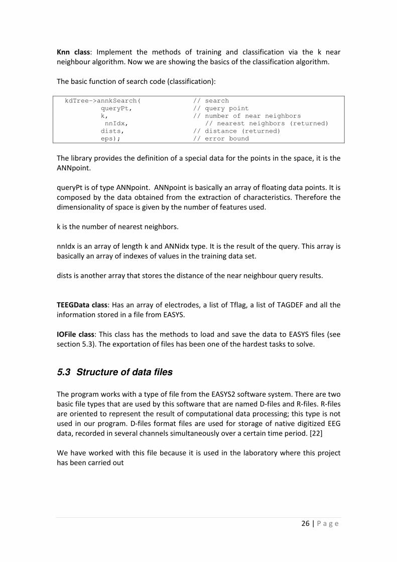
myMath: Some useful functions; Mean, absolute mean, median, variance, standard

deviation, root mean square and line length. These functions perform the appropriate

calculations on a bounded set of data; all have the same declaration structure. The first

parameter ‘a’ is an array of real numbers. The second and third parameters are

respectively the index of the first and last numbers used in the operation, they limit

the range of values in a.

float mean (float *a,

unsigned long int start_position,

unsigned long int finish_position);

Electrode class: In this class is stored the data samples of the channel, the name of the

electrode (see Figure 2 and Figure 3), the number of samples and the frequency of

acquisition among other variables.

The samples acquisitions are stored as a pointer array of float type:

float *data;

Segmentation class: Segmentation class has functions to calculate the number of

samples in each segment, the split points of the segmentation and some additional

functions to perform the concatenation of the flags.

TagTable file: Is not declared as a class but it has two struct definitions; the struct

TAGDEF (Tag definitions) and the struct TFlag (Tag information)

� TAGDEF: The definition of a tag. It contains an abbreviation name for the tag of

2 characters (actually 3 because the endline character ‘\n’ is included), and a

description string (declared as char*).

� TFlag: This struct stores basically the sample position of the tag and the type.

This structures has one important thing, it has defined the operators ‘==’ and

‘<’.

26 | P a g e

Knn class: Implement the methods of training and classification via the k near

neighbour algorithm. Now we are showing the basics of the classification algorithm.

The basic function of search code (classification):

kdTree->annkSearch( // search

queryPt, // query point

k, // number of near neighbors

nnIdx, // nearest neighbors (returned)

dists, // distance (returned)

eps); // error bound

The library provides the definition of a special data for the points in the space, it is the

ANNpoint.

queryPt is of type ANNpoint. ANNpoint is basically an array of floating data points. It is

composed by the data obtained from the extraction of characteristics. Therefore the

dimensionality of space is given by the number of features used.

k is the number of nearest neighbors.

nnIdx is an array of length k and ANNidx type. It is the result of the query. This array is

basically an array of indexes of values in the training data set.

dists is another array that stores the distance of the near neighbour query results.

TEEGData class: Has an array of electrodes, a list of Tflag, a list of TAGDEF and all the

information stored in a file from EASYS.

IOFile class: This class has the methods to load and save the data to EASYS files (see

section 5.3). The exportation of files has been one of the hardest tasks to solve.

5.3 Structure of data files

The program works with a type of file from the EASYS2 software system. There are two

basic file types that are used by this software that are named D-files and R-files. R-files

are oriented to represent the result of computational data processing; this type is not

used in our program. D-files format files are used for storage of native digitized EEG

data, recorded in several channels simultaneously over a certain time period. [22]

We have worked with this file because it is used in the laboratory where this project

has been carried out

27 | P a g e

The standard header file has 11 fields of different types (sizes). Extended header is not

with a fixed definition to provide flexibility; therefore it involves a more tedious

programming. In some areas of the file appendix is necessary to calculate offsets

dynamically. Also, to debug the file resulting by the program is necessary to use a hex

editor. A hex editor is a type of computer program that allows a user to manipulate

binary (normally non-plain text) computer files.

5.3.1 Standard and Extended header

The standard header has 32 bytes long. It contains the signature of the program that

created the data file, the type of the file (D or R), the number of recording channels,

the number of auxiliary channels, the sample frequency (in samples per second), the

total number of data samples in the data section and the scaling factor used in the

data recalibration among others. This data is showed in the Figure 19.

The extended header itself has no fixed structure, compared to the standard header;

rather, it is a chain of different records. The order in which records appear in the

extended header area is indefinite; the extended header area even needs not to be

contiguous.

5.3.2 Tag tables

When a doctor is inspecting the brain waves in a computer program it is useful to have

a way to indicate or comment in a specific point the data that is being examined, that

is to say, place clinical information. For this purpose there are the event markers or

tags.

Standard header

Extended header

Data section

File appendix

0

32

offset

Figure 22. D-File file structure

28 | P a g e

The information related to tags is normally stored into file appendix, following the

data area. The Tag Tables area consists of two parts: the Tag List and the Tag Class

Definitions area. Offsets and lengths of both tables are stated by the TT record of the

extended header. If this record is absent, no tag info is available.

5.4 Adapt/extend the project

In the KNN algorithm we can make interesting modifications. One is to modify the

features that represent the space points. The code is located in the knn.cpp and knn.h

files.

ANNkd_tree is a structure provided by the ann library to create a space of training

points. The declaration is showed in the next code:

kdTree = new ANNkd_tree( // build search structure

dataPts, // the data points

nPts, // number of points

dim); // dimension of space

dataPts is an array of the type defined ANNpoint which is of type ANNcoord*, by

default ANNcoord is defined to be of type double.

In dataPts are stored the points of the space. To calculate the position in the space of

each point there is a function called getFeatures which receives as arguments the

pointer of the EEG data and two more variables that represent the start position and

end position of the segment to process.

Data

from

EEG

Actual segment

last_position

first_position

29 | P a g e

ANNpoint Knn::getFeatures(TEEGData *eeg_data,

unsigned int first_position,

unsigned int last_position) {

ANNcoord f_mean = 0,

f_standard_deviation = 0;

for(int i=0;i<eeg_data->getNumberOfChannels();i++) {

f_mean += (ANNcoord) mean(eeg_data->electrodes[i].data,

first_position,

last_position);

f_standard_deviation += (ANNcoord) standardDeviation(

eeg_data->electrodes[i].data,

first_position,

last_position);

}

ANNpoint ann_point = annAllocPt(dim);

ann_point[0] = f_mean;

ann_point[1] = f_median;

return ann_point;

}

In the code is showed as an example the calculation of the features that make up a

point. It is using two variables to compound it (2-dimension), the mean and standard

deviation.

5.5 Project Settings in Windows

In this section is explained how to set-up and configure the project to have the same

environment as when it was programmed.

First of all, the C/C++ compiler used is the MinGW version 3.4.5 for windows; MinGW

is a port of the GNU Compiler Collection (GCC), and GNU Binutils, for use in the

development of native Microsoft Windows applications [23]. It provides a complete

Open Source programming tool set.

The IDE (integrated development environment) selected was the code::blocks [24]

version 8.02, the latest version released is the 10.05 on 30 May of 2010. Code::block is

an open source environment with several compiler supports and interface GDB [25],

the GNU Project debugger.

The project needs to import the ANN library to use the near neighbour algorithm (see

the section 4.4.1 to know more about this algorithm). There are some precompiled

versions of the library to use with different compilers but to use the library successfully

on Windows using MinGW is necessary to modify the given file ANN.h. This means that

we are using our own compiled version of the library in the project. At line 62 you

30 | P a g e

must comment the next code, leave only uncommented the line with the #define

DLL_API.

// #ifdef WIN32

// #ifdef DLL_EXPORTS

// #define DLL_API __declspec(dllexport)

// #else

// #define DLL_API __declspec(dllimport)

// #endif

// #else

#define DLL_API

// #endif

In code::blocks is possible to link the library automatically. To do it, go to the build

options window, this option is accessible when you click the right mouse button in the

project name (management window). Once you open this window, go to the tab

‘Linker settings’ as shown in Figure 23. Here you have to specify the path to the library.

Figure 23. Build options window of code::blocks IDE

(ANN relative path location).

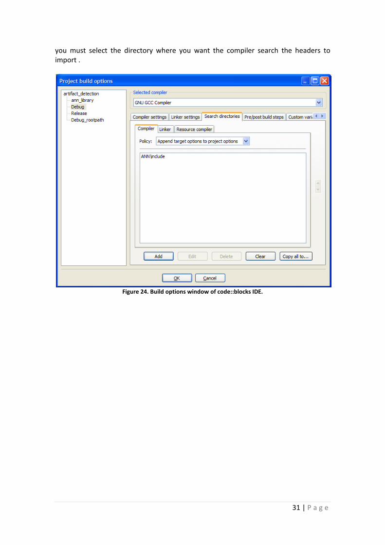
After including the library in the project, the compiler needs to know the available

functions of the library; the header files define that information. ANN has the ANN.h,

ANNperf.h and ANNx.h files.

You must tell to the compiler the location of those files if they are not in the same

folder as the executable. In the same window as before, go to the tab 'Search

directories' as shown in Figure 24 and located in the sub-tab 'Compiler' select 'Add',

31 | P a g e

you must select the directory where you want the compiler search the headers to

import .

Figure 24. Build options window of code::blocks IDE.

32 | P a g e

6 Conclusions

In conclusion we have developed skills in working with pattern recognition methods. In

our case we worked with information obtained from the brain by an EEG. EEG

technology is widely used in cerebral medical diagnostics. An increasing range of

researches are growing using this technology. We have worked in a real research

environment. The data that we have used could be obtained in any laboratory or

hospital.

Our first project was developed in Matlab. The aim has been to focus on some basics

of pattern recognition. We worked to apply segmentation and feature extraction to

improve a future classification of the data. Matlab allows developing algorithms faster

than traditional methods, it has implemented a large number of mathematical

functions and it provides instant access to graphics functions specialized. The works

shows elemental steps to achieve a classification problem.

Our work in C++ has tried to find solutions to the EEG artifacts. It is a common problem

in EEGs. The project developed in C++ can be used as starting point to new projects. It

is ideal for future research in this area that will require speed of execution and

efficient memory management. In addition, there are many compilers for different

platforms using this programming language. For example it is possible to develop such

programs for embedded environments.

33 | P a g e

7 Bibliography

[1] Wikipedia - Cerebral cortex. [Online]. http://en.wikipedia.org/wiki/Cerebral_cortex

[2] Donald E. Read, "Solving deductive-reasoning problems after unilateral temporal

lobectomy. Brain and Language," 1981.

[3] Jaakko Malmivuo and Robert Plonsey, Bioelectromagnetism: Principles and

Applications of Bioelectric and Biomagnetic Fields. New York: Oxford University

Press, 1995.

[4] Health library. [Online]. http://healthlibrary.epnet.com/

[5] Sue Corbett, "Electrode cap," 4537198, August 1985.

[6] Steven C and M.D. Schachter. (2006) Epilepsy.com. [Online].

http://www.epilepsy.com/101/ep101_symptom

[7] Medline Plus. [Online]. http://www.nlm.nih.gov/medlineplus/epilepsy.html

[8] (2000-2010) Talk About Sleep. [Online]. http://www.talkaboutsleep.com/sleep-

disorders/archives/intro.htm

[9] National Institute of Neurological Disorders and Stroke. [Online].

http://www.ninds.nih.gov/disorders/dementias/dementia.htm

[10] (2009) HOPES - Dementia in Huntington's Disease. [Online].

http://hopes.stanford.edu/diagnsis/symptoms/dem2.html

[11] Saeid Sanei and J.A. Chambers, EEG Signal processing. Cardiff, United Kingdom:

John Wiley & Sons, 2007.

[12] Roy Sucholeiki. (2008, November) Normal EEG Waveforms.

[13] Zhaojun Xue, Jia Li, Song Li, and Baikun Wan, "Using ICA to Remove Eye Blink and

Power Line Artifacts in EEG," in Proceedings of the First International Conference on

Innovative Computing, Information and Control, vol. 3, 2006, pp. 107-110.

[14] Brunner DP et al., "Muscle artifacts in the sleep EEG: automated detection and

effect on all-night EEG power spectra," Journal of sleep research, 1996.

[15] D.A. Overton and C. Shagass, "Distribution of eye movement and eye blink

potentials over the scalp," Clinical Neurophysiology, 1969.

[16] Hagemann D and Naumann E, "The effects of ocular artifacts on (lateralized)

broadband power in the EEG," Clinical Neurophysiology, February 2001.

[17] Neuro Care Launches - Common Artifacts in electroencephalography. [Online].

http://www.neurocarelaunches.com/learningex/neurology/ICU/clinical/artifact.htm

[18] IEEE Signal Processing Society. [Online]. http://www.ieee.org.uk/sp.html

[19] Wikipedia. [Online]. http://en.wikipedia.org/wiki/Feature_extraction

[20] Richard L. White,.

[21] Toby Segaran, Programming Collective Intelligence, 1st ed.: O'Reilly Media, Inc.,

2007.

[22] Neuroscience Technology Research, EASYS2 Reference Manual, July 2002.

[23] MinGW compiler. [Online]. http://www.mingw.org

[24] Code:blocks IDE. [Online]. http://www.codeblocks.org

[25] GDB (C/C++ Debugger). [Online]. http://www.gnu.org/software/gdb/

EEG Artifact Detection - pdfs.semanticscholar.org · 7 | Page 3.1 Applications The EEG is indicated...

Documents

Transcript of EEG Artifact Detection - pdfs.semanticscholar.org · 7 | Page 3.1 Applications The EEG is indicated...