Eecurve Ook

8/20/2019 Eecurve Ook

http://slidepdf.com/reader/full/eecurve-ook 1/16

M

LEARNING CURVi

MANUFACTURINI

APPI YIN(":, T~~ LEARNINC

Ich

)a,

IN SERVICE:

:OR

IRV

:ARNING

c:h

iffic:ie

ONS

USING POM FOR WINDOW

LEARNING CURVES

SOLVED PROBLEMS

INTERNET EXERCISES FOR

CURVES

DISCUSSION QUESTIONS

PROBLEMS

CASE STUDY: SMT'S NEGOl

WITH IBM

BIBLIOGRAPHY

.pproach

Arithmetic Approc

Logarithmic Apprc

Learning-Curve Co

STRATEGIC IMPLICAl

LEARNING CURVES

LIMITATIONS OF LEARNI

SUMMARY

KEY TERM

USING EXCEL OM FC

IF

lATIO

G CURVES

:ARNINI



834

MODULE E

LEARNING CURVE

Medical procedure,\' such a.\' heart ,\'urgery,follow a learnin,f,' cunJe, Resear(h indicate,\' thaJ the

death rate ft"om heart transplant,\' drops at a 79% learnin,f,' cun'e, a learnin,f,' rate not unlike

that in many industrial,\'ettin,~s.lt appears that doctor.\, and medical team.\' improl'e, a.\'dn

your odd,\' a,\'a patient. I-t'ith experience. If the death rate i.\' hah'ed el'el}' three operations,

practice may indeed make peifect .

Learning curves

The premise that people

and organizations get

better at their tasks as

the tasks are repeated;

sometimes called

experience curves.

Most organizations Jearn and improve over time. As firnls and employees perfornl a task

over and over, they Jearn how to perform more efficiently. This means that task times and

costs decrease.

Learning curves are based on 1he premise that people and organizations become bet-

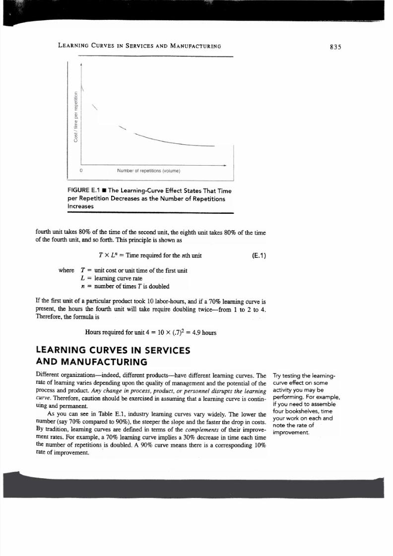
ter at their tasks as the tasks are repeated. A Jearning curve graph (illustrated in Figure

E.1) displays labot-hours per unit versus the number of units produced. From it we see

that the time needed to produce a unit decreases, usually following a negative exponential

curve. as the person or company produces more units. In other words. it takeo le.\'o til11e o

complete each additional unit a .firl11 produces. However, we also see in Figure E.I that

the time .\'avin,~s in completing each subsequent unit decreases. These are the major attri-

butes of the learning curve.

Learning curves were first applied to industry in a report by T. P. Wright of Curtis-

Wright Corp. in 1936.1 Wright described how direct labor costs of making a particular air-

plane decreased with learning. a theory since confirmed by other aircraft manufacturers.

Regardless of the time needed to produce the first plane. learning curves are found to

apply to various categories of air frames (e.g.. jet fighters versus passenger planes versus

bombers). Learning curves have since been applied not only to labor but als() to a wide va-

riety of other costs. including material and purchased components. The power of the

learning curve is so significant that it plays a major role in many strategic decision" re-

lated to employment levels" costs. capacity. and pricing.

The learning curve is based On a d{Juhlin,~ of productivity: That is. when production

doubles. the decrease in time per unit affects the rate of the learIliIl& curve. So. ir the

learning cur\:e is all 80q rate. the second unit takes 80(i( or the time or thc jirst unit. the

p \\ri

I]); tl1



LEARNING CURVES IN SERVICES AND MANUFACTURING

835

FIGURE E.1 .The Learning-Curve Effect States That Time

per Repetition Decreases as the Number of Repetitions

Increases

fourth unit takes 80% of the time of the second unit, the eighth unit takes 80% of the time

of the fourth unit, and so forth. This principle is shown as

(E.1 )

X L n = Time required for the nth unit

where

T = unit cost or unit time of the first unit

L = learning curve rate

n = number of times T is doubled

If the fIrst unit of a particular product took 10 labor-hours, and if a 70% learning curve is

present, the hours the fourth unit will take require doubling twice-,. -from 1 to 2 to 4.

Therefore, the formula is

Hours required for unit 4 = 10 X (.7)2 = 4.9 hours

LEARNING CURVES IN SERVICES

AND MANUFACTURING

Try testing the learning-

curve effect on some

activity you may be

performing. For example,

if you need to assemble

four bookshelves, time

your work on each and

note the rate of

improvement.

Different organizations-indeed, different products-have different learning curves. The

rate of learning varies depending upon the quality of management and the potential of the

process and product. Any change in process, product, or personnel disrupts the learning

CUI"Ve.herefore, caution should be exercised n assuming that a learning curve is contin-

uing and permanent.

As you can see in Table E.l, industry learning curves vary widely. The lower the

number (say 70% compared to 90%), the steeper he slope and the faster the drop in costs.

By tradition, learning curves are defmed in terms of the complements of their improve-

mentrates. For example, a 70% learning curve implies a 30% decrease n time each time

the number of repetitions is doubled. A 90% curve means there is a corresponding 10%

rate of improvement.



:: ;\\c,c """"';

~ "''- ~" ',' ,;I"."

'ift'~\'ft1 tqf,;:':t;t,:~;;~~'

836

MODULE E

LEARNING CURVES

TABLE E.1 .Examples of Learning-Curve Effects

Units produced

Units produced

Number of replacements

86

80

76

1. Model- T Ford production

2. Aircraft assembly

3. Equipment maintenance

atGE

4. Steel production

Price

Direct labor-hours per unit

Average time to replace a

group of parts

Production worker labor-hours

per unit producted

Average price per unit

Average factory selling price

Average price per bit

l-year death rates

Units produced

79

1920-1955

5. Integrated circuits

6. Hand-held calculator

7. Disk memory drives

8. Heart transplants

72a

74

76

79

1964-1972

1975-1978

1975-1978

1985-1988

Units produced

V nits produced

Number of bits

Transplants completed

"Constant dollars.

Sources: James A. Cunnlr)gham, "Using the Learning Curve as a Management Tool," IEEE Spectrum (June 1980): 45. ~ 1980 IEEE;

and David B.Smith andJan LLarsson, "The Impact of Learning on Cost: The Case of Heart Transplantation, "'Hospital and Health

Services Administration (spring 1989): 85-..97.

Failure to consider the

effects of learning can

lead to overestimates of

labor needs and

underestimates of

material needs,

Stable, standardized products and processes tend to have costs that decline more

steeply than others. Between 1920 and 1955, for instance, the steel industry was able to

reduce labor-hours per unit to 79% each time cumulative production doubled.

Learning curves have application in services as well as industry. As was noted in the

caption for the opening photograph, 1-year death rates of heart transplant patients at

Temple University Hospital follow a 79% learning curve. The results of that hospital's

3-year study of 62 patients receiving transplants found that every three operations resulted

in a halving of the 1-year death rate. As more hospitals face pressure from both insurance

companies and the government to enter fixed-price negotiations for their services, their

ability to learn from experience becomes ncreasingly critical. In addition to having appli-

cations in both services and industry, learning curves are useful for a variety of purposes.

These include:

I. Internal labor forecasting, scheduling, establishing costs and budgets.

2. External purchasing and subcontracting (see the SMTcase study at the end of this

module).

3. Strategic evaluation of company and industry performance, including costs and

pricing.

APPLYING THE LEARNING CURVE

A mathematical relationship enables us to express the time it takes to produce a certain

unit. This Telationship is a function of how many units have been produced before the unit

in question and how long it took to produce them. Although this procedure determines

how long it takes to produce a given unit. the consequences of this analysis are more far-

reaching. Costs drop and efficiency goes up for individual firms and the industry.

Therefore. severe problems in scheduling occur if operations are not adjusted for implica-

tions of the learning curve. For instance. if learning-curve improvement is not considered



ApPLYING THE LEARNING CURVE

837

when scheduling, the result may be labor and productive facilities being idle a portion of

the time. Furthermore, firms may refuse additional work because they do not consider the

improvement in their own efficiency that results from learning. From a purchasing per-

spective, our interest is in negotiating what our suppliers' costs should be for further pro-

duction of units based on the size of our order. The foregoing are only a few of the ramifi-

cations of the effect of learning curves.

With this in mind, let us look at three approaches to learning curves: arithmetic analy-

sis, logarithmic analysis, and learning-curve coeff icients.

Although in many cases

analysts can examine

their company and fit a

learning rate to it, trade

journals also publish

industrywide data on

specific types of

operations.

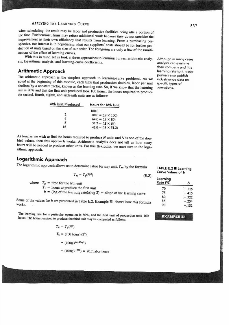
Arithmetic Approach

The arithmetic approach is the simplest approach to learning-curve problems. As we

noted at the beginning of this module, each time that production doubles, labor per unit

declines by a constant factor, known as the learning rate. So, if we know that the learning

rate is 80% and that the fIrst unit produced took] 00 hours, the hours required to produce

the second, ourth, eighth, and sixteenth units are as follows:

Nth Unit Produced

Hours for Nth Unit

2

4

8

16

lOQ.O

80.0 =(;8 X 100)

64.0 = (.8 X 80)

51.2= (;8 X 64)

41.0,= (;8 X 51.2

)

As long as we wish to fmd the hours required to produce N units and N is one of the dou-

bled values, then this approach works. Arithmetic analysis does not tell us how many

hours will be needed to produce other units. For this flexibility, we must turn to the loga-

rithmic approach.

Logarithmic Approach

The logarithmic approach allows us to determine labor for any unit, TN' by the formula

TABLE E.2 .Learning

Curve Values ofb

TN=Tl(Nb)

(E.2)

Learning

Rate (%)

where

b

70

75

80

85

90

-

515

-.415

-.322

-.234

-.152

T N = time for the Nth unit

TI = hours to produce the first uliit

b = (Iog of the learning rate )/(Jog 2) = slope of the learning curve

Some of the values for b are presented in Table E~2.Example El shows how this formula

works.

The learning xatefor a particular operation is 80%, and thefust unit of production took 100

hours. The hours required to produce the third unit may be computed as follows:

TN = T1(Nb)

T3 = (100 hours) (3b)

= (1 OO)(31og .8/1og2)

= (100)(3-'322) 70.2Iabor-ho~



~~"

838

MODULE E

,EARNING CURVES

The logarithmic approach allows us to detennine the hours required for 0/1.\ unit pro

duced, but there is a simpler method.

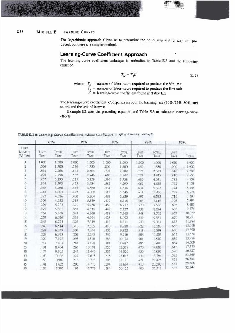
Learning-Curve Coefficient Approach

The leaming-curve coefficient technique is embodied in Table E.3 and the following

equation:

TN = T]C

"E.3)

where

T N = number of labor-hours required to produce the Nth unit

TJ = number of labor-hours required to produce the first unit

C = learning-curve coefficient found in Table E.3

The learning-curve coefficient, C, depends on both the learning rate ao%, 75%, 80%, and

so on) and the unit of interest.

Example E2 uses the preceding equation and Table E.3 to calculate leaming-curve

effects.



ApPL YING THE LEARNING CURVE

839

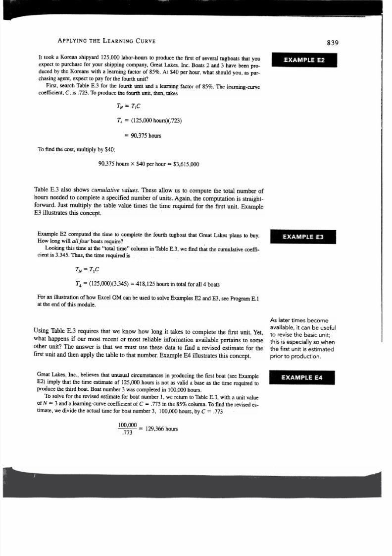
It took a Korean shipyard 125,000 labor-hours to produce the first of several tugboats that you

expect to purchase for your shipping company, Great Lakes, Inc. Boats 2 and 3 have been pro-

duced by the Koreans with a learning factor of 85%. At $40 per hour, what should you, as pur-

chasing agent, expect to pay for the fourth unit?

First, search Table E.3 for the fourth unit and a learning factor of 85%. The learning-curve

coefficient, C, is. 723 Toproduce the fourth unit, then, takes

T N = T]C

T4 = (125,000 hours)(,723)

= 90;375 hours

To find the cost, multiply by $40:

90,375 hours X $40 per hour =$3,615,000

Table E.3 also shows cumulative values. These allow us to compute the total number of

hours needed to complete a specified number of units. Again, the computation is straight-

forward. Just multiply the table value times the time required for the first unit. Example

E3 illustrates this concept.

Example E2 computed the time to complete the fourth tugboat that Great Lakes plans to buy.

How longwillallfour boats require? .

Looking this time at the "total time"column inTableE.3,we find that the cumulativecoeffi-

cientis3.345. Thus, the time required is

TN = TIC

T4={125,0Q0)(3.345) =418,125 hours in1otal for al14 boats

For an llustration ofhow Excel OM can be used to solve Examples E2 andE3, seeProgranlE.l

at the end of this module.

As later times become

available, it can be useful

to revise the basic unit;

this is especially so when

the first unit is estimated

prior to production.

Using Table E.3 requires that we know how long it takes to complete the first unit. Yet,

what happens if our most recent or most reliable inforination available pertains to some

other unit? The answer is that we must use these data to find a revised estimate for the

first unit and then apply the table to that number. Example E4 illustrates this concept.

Great Lakes, Inc., believes that unusual circumstances in producing the first boat (see Example

E2) imply that the time estimate of 125,000 hours is not as valid a base as the time required to

produce the third boat. Boat number 3 was completed in 100,000 hours.

To solve for the revised estimate for boat number I, we return toTable E.3, with a unit value

of N = 3 and a leaming-curve coefficient of C = .773 in the 85% column. To find the revised es-

timate, we divide the actual time for boat number 3, 100,000 hours, by C = .773

100,000

.773

= 129,366 hours



840

MODULE E

LEARNING CURVES

Applications of the

learning curve:

1. Internal ~ determine

labor standards and

rates of material

supply required.

2. External ~ determine

purchase costs.

3. Strategic ~ determine

volume-cost changes.

STRATEGIC IMPLICATIONS

OF LEARNING CURVES

So far, we have shown how operations managers can forecast labor-hour re,quirements or

a product. We have also shown how purchasing agents can determine a supplier's cost,

knowledge that can help in price negotiations. Another important application of learning

curves concerns strategic planning.

An example of a company cost line and industry price line are so labeled in Figure

E.2. These learning curves are straight because both scales are log scales. When the rate

of change is constant, a log-log graph yields a straight line. If an organization believes its

cost line to be the "company cost" line and the industry price is indicated by the das~ed

horizontal line; then the company must have costs at the points below the dotted line (for

example, point a or b) or else operate at a loss (point c).

Lower costs are not automatic; they must be managed down. When a fIrm's strategy

is to pursue a curve steeper than the industry average (the company cost line in Figure

E.2), it does this by

1. Following an aggressive pricing policy.

2. Focusing on continuing cost reduction and productivity improvement.

3. Building on shared experience.

4. Keeping capacity growing ahead of demand.

Costs may drop as a flrn1 pursues the learning curve, but volume must increase for the

learning curve to exist. In recent years, much of the computer industry, for instance, has

operated at a 25% cost reduction per year, with steep learning curves. Texas Instruments

(TI), however, discovered that developing a competitive strategy via the learning curve is

FIGURE E.2 .Industry Learning Curve for Price Compared with

Company Learning Curve for Cost

Note: Both the vertical and horizontal axes of this figure are log scales. This

is known as a log-log graph.



KEY TERMS

841

not for everyone:2 TI allowed other PC producers to lead in cost reductions and price-

cutting. It paid the price for its mistake when sales of its PC line dropped.

Managers must understand competitors before embarking on a learning-curve strat-

egy. Weak competitors are undercapitalized, stuck with high costs, or do not understand

the logic of learning curves. However, strong and dangerous competitors contro] their

costs, have solid financial positions for the large investments needed, and have a track

record of using an aggressive learning-curve strategy. Taking on such a competitor in a

price war may help only the consumer.

LIMITATIONS OF LEARNING CURVES

Before using learning curves, some cautions are in order:

.Because learning curves differ from company to company, as well as industry to in-

dustry, estimates for each organization should be developed rather than applying

someone else's.

.Learning curves are often based on the time necessary to complete the early units;

therefore, those times must be accurate. As current information becomes available,

reevaluation is appropriate.

.Any changes n personnel, design, or procedure can be expected to alter the learning

curve. And the curve may spike up for a short time even if it is going to drop in the

long run.

.While workers and process may improve, the same learning curves do not always

apply to indirect labor and material.

.The culture of the workplace, as well as resource availability and changes in the

process, may alter the learning curve. For instance, as a project nears its end, worker

interest and effort may drop, curtailing progress down the curve.

The learning curve is a powerful tool for the operations manager. This tool can assist op-

erations managers n determining future cost standards or items produced as well as pur-

chased. n addition, the learning curve can provide understanding about company and in-

dustry performance. We saw three approaches to learning curves: arithmetic analysis,

logarithmic analysis, and learning-curve coefficients found in tables. Software can also

help analyze learning curves.

Learning curves (p. 834)

Pankaj Ghemawat, "Building Strategy on the Experience Curve:' Harvard Business Revi~' 63 (March-April

1985): 148.



LEARNING CURVES

USING EXCEL OM FOR LEARNING CURVES

Program E.l shows how Excel OM develops a spreadsheet for leaming-curve calculations.

The input data come from Examples E2 and E3. In cell B7, we enter the unit number for

the base unit (which does not have to be 1), and in B8 we enter the time for this unit.

PROGRAM E.1 .Excel OM's Learning-Curve Module, Using Data from Examples

E2 amd E3

..~

~

USING POM FOR WINDOWS FOR LEARNING CURVES

-

POM for Windows' Learning Curve module computes the length of time that future units

will take, given the time required for the base unit and the learning rate (expressed as a

number between O and 1). As an option, if the times required for the first and Nth unjts are

already known, the learning rate can be computed. SeeAppendix V for further details.

~

SOlVED cPROBLEMS

b) How long will the fIrst 11 systems take in total?

c) As a purchasing agent, you expect to buy units 12

through 15 of the new phone system. What would

be your expected cost for the units if Digicomp

charges $30 for each abor-hour?

Solved Problem E;1

Digicomp produces a new telephone system with built-

in TV screens. ts learning rate is 80%.

a) If the first one took 56 hours, how long will it take

Digicomp1o make the eleventh system?




843

Solution

~ from Table E.3-80% unit time

a) TN = T JC "

T II = (56 hours) (.462) = 25.9 hours

b) Total time for the fIrst I I units = (56 hours)(6.777) = 379.5 hours

from Table E.3-80% unit time ~

c) To find the time for units 12 through 15, we take the total cumu-

lative time for units 1 to 15 and subtract the total t ime for unitsl

to 11, which was computed in part (b). Total time for the first 15

units = (56 hours) (8.511) = 476.6 hours. So, the time for units 12

through 15 is 476.6- 379.5 = 97.1 hours. (This figure could also

be confirmed by computing the times for units 12, 13, 14, and 15

separately using the unit-time column and then adding them.)

Expected cost for units 12 through l5 = (97.1 hours) ($30 per

hour) = $2,913.

Solved Problem E.2

If the fIrst time you perfornI a job takes 60 minutes,

how long will the eighth job take if you are on an 80%

learning curve?

Solution

Three doublings from 1 to 2 to 4 to 8 implies .83. Therefore, we have

60 X (.8)3 = 60 X .512 = 30.72 minutes

or, using Tab1eE.3, we have C = .512. Therefore:

60 X .512=:; 30.72 minutes

Visit ourhomepage atwww.prenhall.com/heizer for these additiona1features'

.Self-test for this module. Practice problems

.Internet exercises. Current articles and research

~


I. What are some of the 1imitations to the use of learn-

ing curves?

2. What techniques can a firm use to move to a steeper

learning curve?

3. What are the approaches to solving learning-curve

problems?

4. Refer to Example E2: What are the implications for

Great Lakes. Inc.. if the engineering department



MODULE E

LEARNING CURVES

wants to change the engine in the third and subse-

quent tugboats that the finn purchases?

Why isn't the learning-curve concept as applicable

in a high-volume assembly line as it is in most other

human activities?

6. What can cause a learning curve to vary from

smooth downward slope?

7. Explain the concept of the "doubling'. effect in

learning curves.

PROBLEMS*

~

E.l

~

E.2

~

E.3

~. E.4

~ : E.5

~: E.6

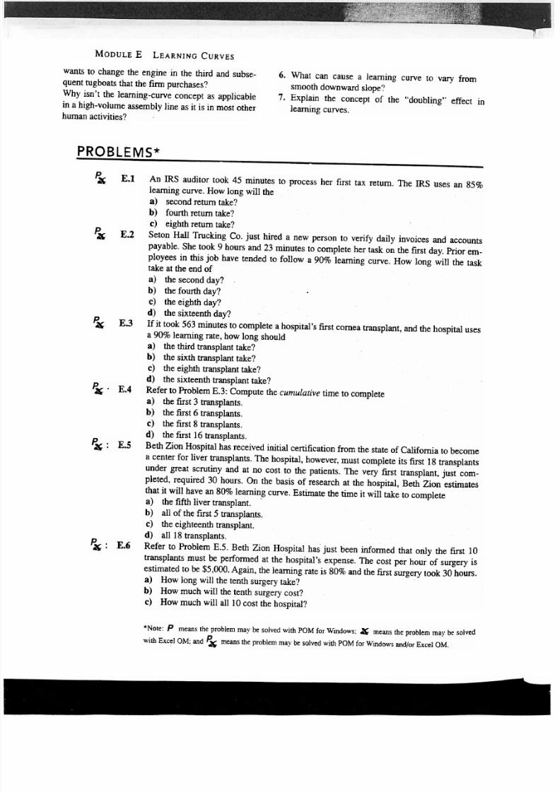
An IRS auditor took 45 minutes to process her fIrst tax return. The IRS uses an 85%

learning curve. How long will the

a) second return take?

b) fourth return take?

c) eighth return take?

Seton Hall Trucking Co. just hired a new person to verify daily invoices and accounts

payable. She took 9 hours and 23 minutes to complete her task on the fIrSt day. Prior em-

ployees in this job have tended to follow a 90% learning curve. How long will the task

take at the end of

a) the second day?

b) the fourth day?

c) the eighth day?

d) the sixteenth day?

If it took 563 minutes to complete a hospital's first cornea transplant, and the hospital uses

a 90% learning rate, how long should

a) the third transplant take?

b) the sixth transplant take?

c) the eighth transplant take?

d) the sixteenth transplant take?

Refer to Problem E.3: Compute the cumulative time to complete

a) the fIrst 3 transplants.

b) the first 6 transplants.

c) the first 8 transplants.

d) the fIrst 16 transplants.

Beth Zion Hospital has received initial certification from the state of California to become

a center for liver transplants. The hospital, however, must complete its first 18 transplants

under great scrutiny and at no cost to the patients. The very fIrst transplant, just com-

pleted, required 30 hours. On the basis of research at the hospital, Beth Zion estimates

that it will have an 80% learning curve. Estimate the time it will take to complete

a) the f1fth liver transplant. .

b) all of the fIrst 5 transplants.

c) the eighteenth transplant.

d) all 18 transplants.

Refer to Problem E.5. Beth Zion Hospital has just been informed that orily the fIrst 10

transplants must be performed at the hospital s expense. The cost per hour of surgery is

estimated to be $5,000. Again, the learning rate is 80% and the fIrst surgery took 30 hours.

a) How long will the tenth surgery take?

b) How much will the tenth surgery cost?

c) How much will all 10 cost the hospital?

*Note: p means the problem may be sojved with POM for Windows; 4(; means the problem may be solved

with Excel OM; and ~ means the problem may be solved with POM for Windows and/or Excel OM.



PROBLEMS

845

E.7

E.8

E.9

E.I0

E.ll

~:

E.l2

~: E.13

E.14

~

E.15

E.16

~

E.17

E.18

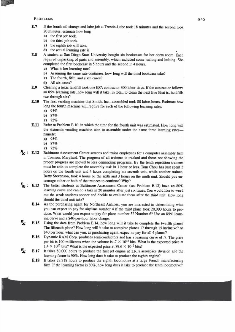
If the fourth oil change and lube job at Trendo-Lube took 18 minutes and the second took

20 minutes, estimate how long

a) the first job took.

b) the third job took.

c) the eighth job will take.

d) the actual learning rate is.

A student at San Diego State University bought six bookcases for her dorm room. Each

required unpacking of parts and assembly. which included some nailing and bolting. She

completed the first bookcase in 5 hours and the second in 4 hours.

a) What is her learning rate?

b) Assuming the same rate continues, how long will the third bookcase take?

c) The fourth, fifth, and sixth cases?

d) All six cases?

Cleaning a toxic landfill took one EPA contractor 300 labor-days. If the contractor follows

an 85% learning rate, how long will it take, in total, to clean the next five (that is, landfills

two through six)?

The first vending machine that Smith, Inc., assembled took 80 labor-hours. Estimate how

long the fourth machine will require for each of the following learning rates:

a) 95%

b) 87%

c) 72%

Refer to Problem E.IO, in which the time for the fourth unit was estimated. How long will

the sixteenth vending machine take to assemble under the same three learning rates-

namely:

a) 95%

b) 87%

c) 72%

Baltimore Assessment Center screens and trains employees for a computer assembly fIrm

in Towson, Maryland. The progress of all trainees is tracked and those not showing the

proper progress are moved to less demanding programs. By the tenth repetition trainees

must be able to complete the assembly task in 1 hour or less. Tom Chou has ust spent 5

hours on the fourth unit and 4 hours completing his seventh unit, while another trainee,

Betty Stevenson, took 4 hours on the sixth and 3 hours on the ninth unit. Should you en-

courage either or both of the trainees to continue? Why?

The better students at Baltimore Assessment Center (see Problem E;12) have an 80%

learning curve and can do a task in 20 minutes after just six times. You would like to weed

out the weak students sooner and decide to evaluate them after the third unit. How long

should the third unit take?

As the purchasing agent for Northeast Airlines, you are interested in determining what

you can expect to pay for airplane number 4 if the third plane took 20,000 hours to pro-

duce. What would you expect to pay for plane number 5? Number 6? Use an 85% learn-

ingcurve and a $40-per-hour labor charge.

Using the data from Problem E.14, how long will it take to complete the twelfth plane?

The fifteenth plane? How long will it take to complete planes 12 through 15 inclusive? At

$40 per hour, what can you, as purchasing agent, expect to pay for alJ 4 planes?

Dynamic RAM Corp. produces semiconductors and has a learning curve of. 7. The price

per bit is 100 millicents when the volume is. 7 X 1012bits. What is the expected price at

1.4 X 1012bits? What is the expected price at 89.6 X 1012bits?

It takes 80,000 hours to produce the first jet engine at T.R.'s aerospace division and the

learning factor is 90%. How long does it take to produce the eighth engine?

It takes 28,718 hours to produce the eighth locomotive at a large French manufacturing

firm. If the learning factor is 80%, how long does it take to produce the tenth locomotive?



846

MODULE E

LEARNING CURVES

~

E.19

~

E.20

: E.21

If the first unit of a production run takes 1 hour and the fInn is on an 80% learning curve.

how long will unit 100 take? (Hint: Apply the coefficient in Table E.3 on p. 838, twice.)

As the estimator for Umble Enterprises, your job is to prepare an estimate for a potential

customer service contract. The contract is for the service of dieseJ Jocomotive cyJinder

heads. The shop has done some of these in the past on a sporadit, basis. The time re-

quired to service each cyJinder head has been exactly 4 hours, and similar work has been

accomplished at an 85% learning curve. The customer wants you to quote in batches of

12 and 20.

a) Prepare the quote.

b) After preparing the quote, you find a labor ticket for this customer for five locomotive

cylinder heads. From the sundry notations on the labor ticket, you concJude that the

fifth unit took 2.5 hours. What do you conclude about the learning curve and your

quote?

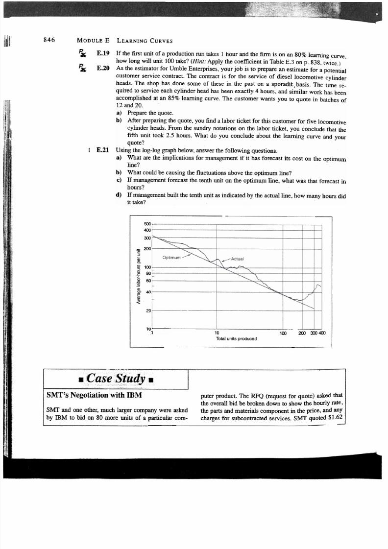
Using the log-log graph below, answer the following questions.

a) What are the implications for management if it has forecast its cost on the optimum

line?

b) What could be causing the fluctuations above the optimum line?

c) If management forecast the tenth unit on the optimum line, what was that forecast in

hours?

d) If management built the tenth unit as ndicated by the actual line, how many hours did

it take?

500..-

400

300

.2

"

0;

0.

f

"

o

.r:

~

O

.0

~

0>

01

~

0>

~

200

100

80

60

40

20

10' .

1

2(XJ 300 400

00

0

Total units produced

SMT's Negotiation with mM

puter product. The RFQ (request for quote) asked that

the overall bid be broken down to show the hourly rate

the parts and materials component in the price, and any

charges for subcontracted services. SMT quoted $1.62

SMT and one other, much larger company were asked

by IBM to bid on 80 more units of a particular com-



CASE STUDY

847

At this point. SMT representatives expressed great

concern about the possibility of inflation in materials

costs. The IBM negotiators volunteer'ep to include a

form of price escalation in the contract, as previously

agreed among themselves. IBM representatives sug-

gested that if overall materials costs changed by more

than 10%. the price could be adjusted accordingly.

However, if one party took the initiative to have the

price revised, the other could require an analysis of all

[arts and materials invoices in arriving at the new

pnce.

Another concern of the SMT representatives was

that a large amount of overtime and subcontracting

would be required to meet IBM's specified delivery

schedule. IBM negotiators thought that a relaxation in

the delivery schedule might be possible if a price con-

cession could be obtained. In response, the SMT team

offered a 5% discount, and this was accepted. As a re-

sult of these negotiations, the SMT price was reduced

almost 20% below its original bid price.

In a subsequent meeting called to negotiate the

prices of certain pipes to be used in the system, it be-

came apparent to an IBM cost estimator that SMT

representatives had seriously underestimated their

costs. He pointed out this apparent error because he

could not understand why SMT had quoted such a

low figure. He wanted to be sure that SMT was using

the correct manufacturing process. In any case, if

SMT estimators had made a mistake, it should be

l

oted. It was IBM's policy to seek a fair price both for

itself and for its suppliers. IBM procurement man-

agers believ~d that if a vendor was losing money on a

job, there would be a tendency to cut comers. In addi-

tion, the IBM negotiator felt that by pointing out the

error, he generated some goodwill that would help in

future sessions.

Discussion Questions

million and supplied the cost breakdown as requested.

The second company submitted only one tota] figure,

$5 million, with no cost breakdown. The decision was

made to negotiate with SMT.

The IBM negotiating team included two purchas-

ing managers and two cost engineers. One cost engi-

neer had developed manufacturing cost estimates for

every component, working from enginee ing drawings

and cost-data books that he had built up from previous

experience and that contained time factors, both setup

and run times, for a large variety of operations. He es-

timated materials costs by working both from data

supplied by the IBM corporate purchasing staff and

from purchasing journals. He visited SMT facilities to

see the tooling available so that he would know what

processes were being used. He assumed that there

would be perfect conditions and trained operators,

and he developed cost estimates for the 158th unit

{previous orders were for 25, 15, and 38 units). He

added 5% for scrap-and-flow loss; 2% for the use of

temporary tools, jigs, and fixtures; 5% for quality

control; and 9% for purchasing burden. Then, using

an 85% learning curve, he backed up his costs to get

an estimate for the first unit. He next checked the data

on hours and materials for the 25, 15, and ?8 units al-

ready made and found that his estimate for the first

unit was within 4% of actual cost. His check, how-

ever, had indicated a 90% leaming-curve effect on

hours per unit.

In the negotiations, SMT was rep esented by one

of the two owners of the business, two engineers, and

one cost estimator. The sessions opened with a discus-

sion of learning curves. The IBM cost estimator

demonstrated that SMT had in fact been operating on a

90% learning curve. But, he argued, it should be possi-

ble to move to an 85% curve, given the longer runs, re-

duced setup time, and increased continuity of workers

on the job that would be possible with an order for 80

units. The owner agreed with this analysis and was

wining to reduce his price by 4%.

However, as each operation in the manufacturing

process was discussed, it became clear that some

IBM cost estimates were too low because certain

crating and shipping expenses had been overlooked.

These oversights were minor, however, and in the

following discussions, the two parties arrived at a

common understanding of specifications and reached

agreements on the costs of each manufacturing

operation.

1. What are the advantages and disadvantages to IBM

and SMT from this approach?

2. How does SMT's proposed learning rate compare

with that of other companies?

3. What are the limitations of the learning curve in

this case?

Sollrce: Adapted from E. Raymond Corey. Procllremenl

Mana,~emenl: Slrale.~.I. Or iOni:alion, and Decision Maki1l,~ (New

York. Van Nostrand Reinhold).



MODULE E

LEARNING CURVES

BIBLIOGRAPHY

Smith, J., Learning Curve for Cost, Control. Industrial

Engineering and Management Press, Institute of lndus-

trial Engineers. Norcross, Georgia (1998).

Taylor, M. L. "The Learning Curve-A Basic Cost Projection

Tool." N.A.A. Bulletin (February 1961): 21-26.

Zangwil1, W. I., and r. B. Kantor. "Toward a Theory of

Continuous Improvement and the Learning Curve.

Management Science 44, no.7 (July 1998): 910-920.

Abernathy, W. J., and K. Wayne. "Limits of the Learning

Curve." Harvard Business Revie\1'52 (September-October

1974): 109-119.

Carom, J. "A Note on Learning Curve Parameters:' Decision

Sciences (summer 1985): 325-327.

Hall, G., and S. Howell. "The Experience Curve from the

Economist's Perspective." Strategic Management Journal,

(July-September 1985): 197-210.

Hart, C. W., G. Spizizen, and D. D. Wyckoff. "Scale

Economies and the Experience Curve." The Cornell

H.RA. Quarterly 25 (May 1984): 91-103.

Eecurve Ook

Documents

Transcript of Eecurve Ook