EE40 Lecture 12 Venkat Anantharamee40/sp08/lectures/EE40_Spring08_Lecture12.pdfEE40 Spring 2008...
25
Slide 1 EE40 Spring 2008 Venkat Anantharam EE40 Lecture 12 Venkat Anantharam 2/20/08 Reading: Chap. 4: first order circuits
Transcript of EE40 Lecture 12 Venkat Anantharamee40/sp08/lectures/EE40_Spring08_Lecture12.pdfEE40 Spring 2008...

Slide 1EE40 Spring 2008 Venkat Anantharam
EE40Lecture 12
Venkat Anantharam
2/20/08 Reading: Chap. 4: first order
circuits

Slide 2EE40 Spring 2008 Venkat Anantharam
First Order Circuits
R+
-Cvs(t)
+-vc(t)
+ -vr(t)ic(t)
vL(t)is(t) R L
+
-
iL(t)
KVL around the loop: KCL at the node:
( ) ( ) ( )cc s
dv tRC v t v tdt
+ = ( ) ( ) ( )LL s
di tL i t i tR dt
+ =
Slide 3EE40 Spring 2008 Venkat Anantharam
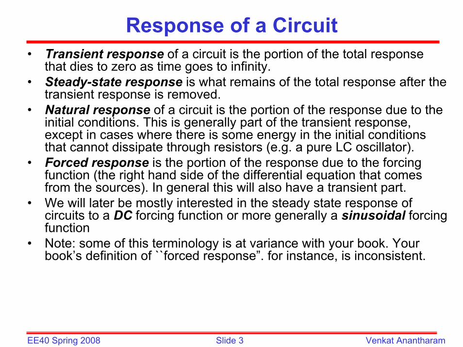
Response of a Circuit• Transient response of a circuit is the portion of the total response
that dies to zero as time goes to infinity.• Steady-state response is what remains of the total response after the
transient response is removed.• Natural response of a circuit is the portion of the response due to the
initial conditions. This is generally part of the transient response, except in cases where there is some energy in the initial conditions that cannot dissipate through resistors (e.g. a pure LC oscillator).
• Forced response is the portion of the response due to the forcing function (the right hand side of the differential equation that comes from the sources). In general this will also have a transient part.
• We will later be mostly interested in the steady state response of circuits to a DC forcing function or more generally a sinusoidal forcing function
• Note: some of this terminology is at variance with your book. Your book’s definition of ``forced response”. for instance, is inconsistent.
Slide 4EE40 Spring 2008 Venkat Anantharam
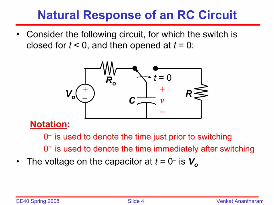
Natural Response of an RC Circuit• Consider the following circuit, for which the switch is
closed for t < 0, and then opened at t = 0:
Notation:0– is used to denote the time just prior to switching0+ is used to denote the time immediately after switching
• The voltage on the capacitor at t = 0– is Vo
C
Ro
Vo R
t = 0+−
+v–

Slide 5EE40 Spring 2008 Venkat Anantharam
Solving for the Voltage (t ≥ 0)
• For t > 0, the circuit reduces to
• Applying KCL to the RC circuit:
• Solution:
+
v
–
RCtetv /o V)( −=
CRo
Vo R+−
i

Slide 6EE40 Spring 2008 Venkat Anantharam
Solving for the Current (t > 0)
• Note that the current changes abruptly:
RCtoeVtv /)( −=
RVi
eRV
Rvtit
i
o
RCto
=⇒
==>
=
+
−
−
)0(
)( 0,for
0)0(
/
+
v
–
CRo
Vo R+−
i
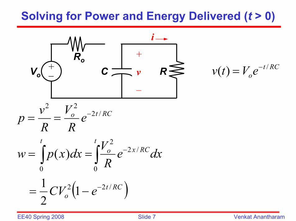
Slide 7EE40 Spring 2008 Venkat Anantharam
Solving for Power and Energy Delivered (t > 0)
( )RCto
tRCxo
t
RCto
eCV
dxeRVdxxpw
eRV
Rvp
/22
0
/22
0
/222
121
)(
−
−
−
−=
==
==
∫∫
RCtoeVtv /)( −=
+
v
–
CRo
Vo R+−
i

Slide 8EE40 Spring 2008 Venkat Anantharam
Natural Response of an RL Circuit• Consider the following circuit, for which the switch is
closed for t < 0, and then opened at t = 0:
Notation:0– is used to denote the time just prior to switching0+ is used to denote the time immediately after switching
• t<0 the entire system is at steady-state; and the inductor is like short circuit
• The current flowing in the inductor at t = 0– is Io and V across is 0.
LRo
t = 0 i +
v
–Io R

Slide 9EE40 Spring 2008 Venkat Anantharam
Solving for the Current (t ≥ 0)• For t > 0, the circuit reduces to
• Applying KVL to the LR circuit:• v(t)=i(t)R• At t=0+, i=I0, • At arbitrary t>0, i=i(t) and
• Solution:
( )( ) di tv t Ldt
=
LRo
i +
v
–Io R
-
= I0e-(R/L)ttLReiti )/()0()( −=

Slide 10EE40 Spring 2008 Venkat Anantharam
Solving for the Voltage (t > 0)
tLRoeIti )/()( −=
• Note that the voltage changes abruptly:
LRo
+
v
–Io R
I0Rv
ReIiRtvtv
tLRo
=⇒
==>
=
+
−
−
)0(
)(0,for 0)0(
)/(

Slide 11EE40 Spring 2008 Venkat Anantharam
Solving for Power and Energy Delivered (t > 0)tLR
oeIti )/()( −=
LRo
+
v
–Io R
( )tLRo
txLR
o
t
tLRo
eLI
dxReIdxxpw
ReIRip
)/(22
0
)/(22
0
)/(222
121
)(
−
−
−
−=
==
==
∫∫
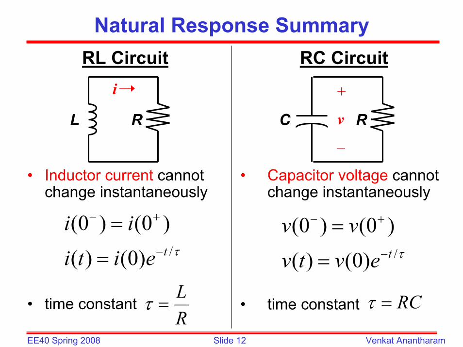
Slide 12EE40 Spring 2008 Venkat Anantharam
Natural Response SummaryRC Circuit
• Capacitor voltage cannot change instantaneously
• time constant
RL Circuit
• Inductor current cannot change instantaneously
• time constantRL
=τ
τ/)0()()0()0(teiti
ii−
+−
=
=
R
i
L
+
v
–
RC
τ/)0()()0()0(tevtv
vv−
+−
=
=
RC=τ

Slide 13EE40 Spring 2008 Venkat Anantharam
Digital SignalsWe compute with pulses.
We send beautiful pulses in:
time
volta
ge
time
volta
ge
But we receive lousy-looking pulses at the output:
Capacitor charging effects are responsible!
• Every node in a real circuit has capacitance; it’s the charging of these capacitances that limits circuit performance (speed)

Slide 14EE40 Spring 2008 Venkat Anantharam
Pulse DistortionR The input voltage pulse
width must be large enough; otherwise the output pulse is distorted.(We need to wait for the output to reach a recognizable logic level, before changing the input again.)
0123456
0 1 2 3 4 5Time
Vout
Pulse width = 0.1RC
0123456
0 1 2 3 4 5Time
Vout
0123456
0 5 10 15 20 25Time
Vout
+
Vout–
Vin(t) C+
–
Pulse width = RC Pulse width = 10RC

Slide 15EE40 Spring 2008 Venkat Anantharam
Example
Vin
RVout
C
Suppose a voltage pulse of width5 µs and height 4 V is applied to theinput of this circuit beginning at t = 0:
R = 2.5 kΩC = 1 nFτ = RC = 2.5 µs
• First, Vout will increase exponentially toward 4 V.• When Vin goes back down, Vout will decrease exponentially
back down to 0 V.
What is the peak value of Vout?
The output increases for 5 µs, or 2 time constants.It reaches 1-e-2 or 86% of the final value.
0.86 x 4 V = 3.44 V is the peak value

Slide 16EE40 Spring 2008 Venkat Anantharam
First Order Circuits: Forced Response
R+
-Cvs(t)
+-vc(t)
+ -vr(t)ic(t)
vL(t)is(t) R L
+
-
iL(t)
KVL around the loop:vr(t) + vc(t) = vs(t) )()(1)( tidxxv
LRtv
s
t
=+ ∫∞−
KCL at the node:
( ) ( ) ( )LL s
di tL i t i tR dt
+ =
( ) ( ) ( )cc s
dv tRC v t v tdt
+ =

Slide 17EE40 Spring 2008 Venkat Anantharam
Complete Solution• Voltages and currents in a 1st order circuit satisfy a
differential equation of the form
– f(t) is called the forcing function.• The complete solution is the sum of any particular solution and the
associated complementary solution
– Particular solution is any solution that satisfies the original equation.– Complementary solution is a solution of the homogeneous equation (the
one with zero forcing function) used to satisfy the initial conditions. In effect it also compensates for the value of the particular solution at 0.
( )( ) ( )dx tx t f tdt
τ+ =
/
( )( ) 0
( )
cc
tc
dx tx tdt
x t Ke τ
τ
−
+ =
=
( )( ) ( )pp
dx tx t f t
dtτ+ = Homogeneous
equation
( ) ( ) ( )p cx t x t x t= +
Original equation Solution to the homogeneous equation.

Slide 18EE40 Spring 2008 Venkat Anantharam
The Time Constant
• The complementary solution for any 1st order circuit looks like, for some K,
• For an RC circuit, τ = RC• For an RL circuit, τ = L/R
/( ) tcx t Ke τ−=

Slide 19EE40 Spring 2008 Venkat Anantharam
What Does Xc(t) Look Like?
τ = 10-4/( ) tcx t e τ−=
• τ is the amount of time necessary for an exponential to decay to 36.7% of its initial value.
• -1/τ is the initial slope of an exponential with an initial value of 1.

Slide 20EE40 Spring 2008 Venkat Anantharam
Particular Solution• A particular solution xp(t) is usually found as a
weighted sum of f(t) and its first derivative.• For example, if f(t) is constant (DC forcing
function), then xp(t) can be taken to be a constant.
• If f(t) is sinusoidal, then xp(t) can be taken to be sinusoidal.
• Note: The notion of ``particular solution” is not unique. Any solution of the homogeneous equation can be added to a particular solution to give another particular solution! The corresponding complementary solution would then adjust accordingly to give the same total response for the given initial conditions.

Slide 21EE40 Spring 2008 Venkat Anantharam
Particular Solution: F(t) Constant
Fdttdxtx P
P =+)()( τ
Guess a solutionBtAtxP +=)(
FdtBtAdBtA =
+++
)()( τ
Equation holds for all time and thus each coefficient is
individually zero
FBBtA =++ τ)(
0)()( =+−+ tBFBA τ
0)( =−+ FBA τ0)( =B
FA =0=B

Slide 22EE40 Spring 2008 Venkat Anantharam
The Particular Solution: F(t) Sinusoid)cos()sin()()( wtFwtF
dttdxtx BA
PP +=+τ
Guess a solution )cos()sin()( wtBwtAtxP +=
)cos()sin())cos()sin(())cos()sin(( wtFwtFdt
wtBwtAdwtBwtA BA +=+
++ τ
Equation holds for all time and \thus each coefficient is
individually zero
( )sin( ) ( )cos( ) 0A BA B F t B A F tτω ω τω ω− − + + − =( ) 0BB A Fτω+ − =( ) 0AA B Fτω− − =
2( ) 1A BF FA τωτω+
=+ 2( ) 1
A BF FB τωτω
−= −
+
2 2 2
1
2
1 1( ) sin( ) cos( )( ) 1 ( ) 1 ( ) 1
1 cos( ); tan ( )( ) 1
Px t t t
t where
τω ω ωτω τω τω
ω θ θ τωτω
−
⎡ ⎤= +⎢ ⎥
⎢ ⎥+ + +⎣ ⎦
= − =+

Slide 23EE40 Spring 2008 Venkat Anantharam
The Particular Solution: F(t) Exp.
21)()( FeF
dttdxtx tP
P +=+ −ατGuess a solution
21)()( FeF
dtBeAdBeA t
tt +=
+++ −
−− α
αα τt
P BeAtx α−+=)(
Equation holds for all time and thus each coefficient is
individually zero21)( FeFBeBeA ttt +=−+ −−− ααα ατ
0)()( 12 =−−+− − teFBFA αατ
0)( 2 =− FA0)( 1 =−− FB ατ
2FA =1FB +=ατ

Slide 24EE40 Spring 2008 Venkat Anantharam
The Total Solution: F(t) Sinusoid
)cos()sin()( wtBwtAtxP +=
)cos()sin()()( wtFwtFdttdxtx BA
PP +=+τ
2( ) 1A BF FA τωτω+
=+ 2( ) 1
A BF FB τωτω
−= −
+
τt
C Ketx −=)(
τt
T KewtBwtAtx −++= )cos()sin()(
Only K is unknown and is determined by the
initial condition at t =0 Example: xT(t=0) = VC(t=0)
)0()0cos()0sin()0(0
==++=− tVKeBAx CT
τ
)0()0( ==+= tVKBx CT BtVK C −== )0(

Slide 25EE40 Spring 2008 Venkat Anantharam
Example
C
RVs
t = 0+−
+vc–
• Given vc(0-)=1, Vs=2 cos(ωt), ω=200.• Find i(t), vc(t)=?