EE392m Fault Diagnostics Systems...
35
2009 Gorinevsky Fault Diagnostics Systems 1 EE392m EE392m Fault Diagnostics Systems Fault Diagnostics Systems Introduction Introduction Dimitry Gorinevsky Consulting Professor Information Systems Laboratory E392m ● Spring 2009
Transcript of EE392m Fault Diagnostics Systems...

2009Gorinevsky
Fault Diagnostics Systems 1
EE392m EE392m Fault Diagnostics Systems Fault Diagnostics Systems
Introduction Introduction Dimitry Gorinevsky Consulting Professor
Information Systems Laboratory
E392m ● Spring 2009
2009Gorinevsky
Fault Diagnostics Systems 2
Course Subject
• Engineering of fault diagnostics systems • Embedded computer interacting with real world
– Detect abnormal operation – Fault tolerance: more than 80% of critical control code
• Operations and maintenance – More than 50% of the system lifetime costs – Troubleshooting support – Condition-based maintenance – CBM

2009Gorinevsky
Fault Diagnostics Systems 3
Prerequisites and Course Place
• The subject is not covered in other courses• Prerequisites (helpful but not necessary)
– Stat 116; EE263 or Eng 207a; EE278 or Eng 207b
• The course is about technical approaches that are actually used in fault diagnostics applications – Survived demands of real life – Used and supported by BS-level engineers in industry – Should be accessible to a Stanford grad student

2009Gorinevsky
Fault Diagnostics Systems 4
Course Mechanics • Class website: www.stanford.edu/class/ee392M/• Weekly seminars
– Follow website announcements • Guest lecturers from diverse industries
– Co-sponsored by NASA • Travel support for lecturers
– Lecture notes will be posted as available• Attendance • Reference texts
– Isermann; Chiang, Russel, & Braatz; Patton, Clark & Frank– Different coverage – Contact me if you have a specific interest

2009Gorinevsky
Fault Diagnostics Systems 5
On-line (Embedded) Functions
• Embedded system, anomaly warnings – BIT – Built-in-Test– BITE – Built-in-Test Equipment
• FDIR – Fault Detection Identification and Recovery
• FT-RM– Fault Tolerance and Redundancy Management

2009Gorinevsky
Fault Diagnostics Systems 6
Off-line Functions• Reliability
– FMECA- Failure Mode, Effects, and Criticality Analysis – Design time analysis – open loop
• Maintenance and Support – Diagnostics for maintenance– Troubleshooting support– Test equipment – CBM – Condition Based Maintenance– Pre-testing – disk drives

2009Gorinevsky
Fault Diagnostics Systems 7
Fault Diagnostics in Industry• Space systems • Defense systems: aviation, marine, and ground • Commercial aerospace
– Aircraft, jet engines • Ground vehicles
– Locomotives, trucks, cars• High-tech
– Networks and IT systems – Disk drives– Server farms
• Process control– IC Manufacturing– Refineries– Power plants
• Oil and gas drilling
2009Gorinevsky
Fault Diagnostics Systems 8
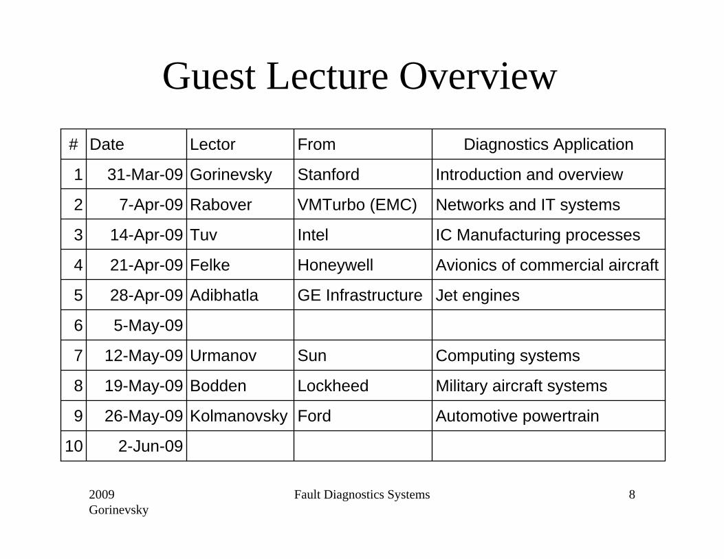
Guest Lecture Overview
Automotive powertrain
Military aircraft systems
Computing systems
Jet engines
Avionics of commercial aircraft
IC Manufacturing processes
Networks and IT systems
Introduction and overview
Diagnostics Application
2-Jun-0910
FordKolmanovsky26-May-099
LockheedBodden19-May-098
SunUrmanov12-May-097
5-May-096
GE InfrastructureAdibhatla28-Apr-095
HoneywellFelke21-Apr-094
IntelTuv14-Apr-093
VMTurbo (EMC) Rabover7-Apr-092
StanfordGorinevsky31-Mar-091
From LectorDate#
2009Gorinevsky
Fault Diagnostics Systems 9
Diagnostics Methods Overview
• Shewhart chart (Control chart)• Multivariable SPC, T2
• Model-based estimation – Least squares estimation
• Integrated diagnostics – Cascaded design

2009Gorinevsky
Fault Diagnostics Systems 10
Abnormality Detection - SPC
• SPC - Statistical Process Control – monitoring of manufacturing processes– warning for off-target quality
• Main SPC method – Shewhart Chart (1920s)
• Also see – EWMA (1940s)– CuSum (1950s) – Western Electric Rules (1950s)
2009Gorinevsky
Fault Diagnostics Systems 11
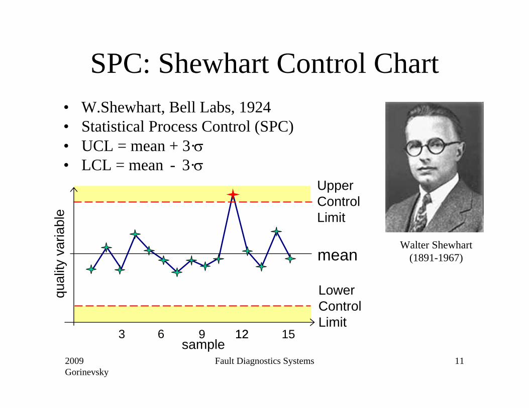
SPC: Shewhart Control Chart• W.Shewhart, Bell Labs, 1924• Statistical Process Control (SPC) • UCL = mean + 3·σ• LCL = mean - 3·σ
Walter Shewhart (1891-1967)
sample3 6 9 1212 15
mean
qual
ity v
aria
ble
Lower Control Limit
Upper Control Limit

2009Gorinevsky
Fault Diagnostics Systems 12
Shewhart Chart, cont’d• Quality variable assumed randomly
changing around a steady state value• Detection: y(t) > UCL=mean+3·σ• For normal distribution, false alarm
probability is less than 0.27%
P(e > 3) = 1-Φ(3) = 0.1350·10-2
P(e < 3) = Φ(-3) = 0.1350·10-2
σµ0)()( −
=tyte
UCLLCL
2009Gorinevsky
Fault Diagnostics Systems 13
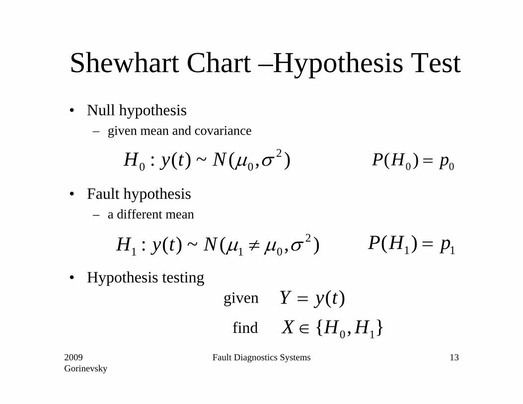
Shewhart Chart –Hypothesis Test• Null hypothesis
– given mean and covariance
• Fault hypothesis– a different mean
• Hypothesis testing
),(~)(: 200 σµNtyH
),(~)(: 2011 σµµ ≠NtyH
},{)(
10 HHXtyY
∈=given
find
00 )( pHP =
11)( pHP =

2009Gorinevsky
Fault Diagnostics Systems 14
Bayesian Formulation • Data:
• Bayes rule
• Observation model:• Prior model:• Maximum A posteriori Probability estimate
XY Observation
Underlying State
c XPXYPYXP ⋅⋅= )()|()|()|( XYP
)(XP
( ) ( )( )4444 34444 21
indexposterior log
log|logminarg−−
−−=L
XPXYPX
Rev. Thomas Bayes(1702-1761)
2009Gorinevsky
Fault Diagnostics Systems 15
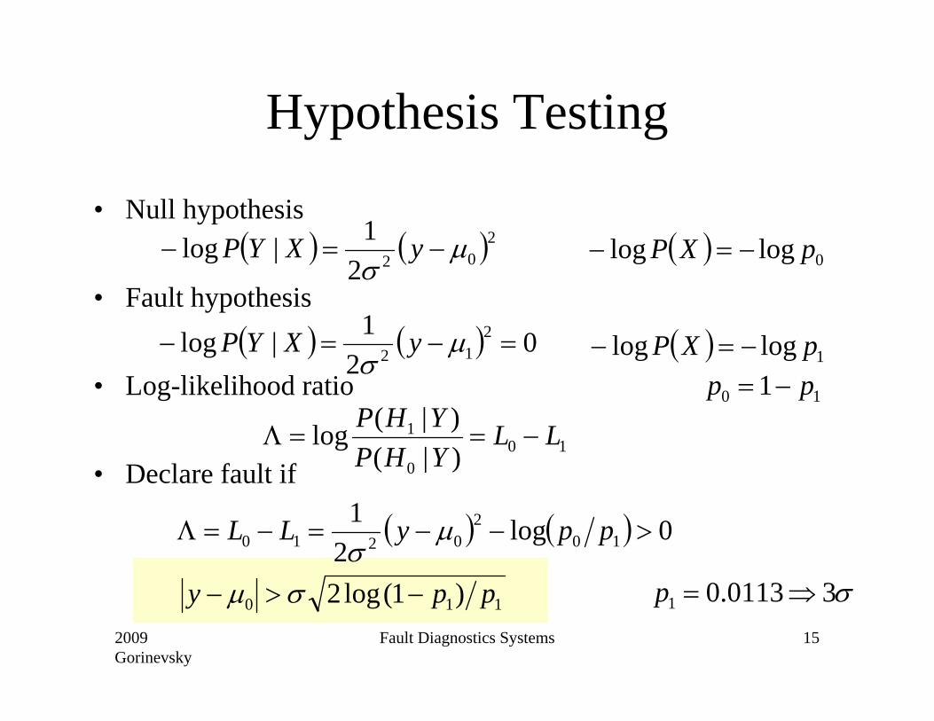
Hypothesis Testing
• Null hypothesis
• Fault hypothesis
• Log-likelihood ratio
• Declare fault if
( ) ( )20221|log µσ
−=− yXYP ( ) 0loglog pXP −=−
( ) ( ) 02
1|log 212 =−=− µ
σyXYP ( ) 1loglog pXP −=−
( ) ( ) 0log2
110
20210 >−−=−=Λ ppyLL µ
σ
110 )1(log2 ppy −>− σµ
10 1 pp −=
σ30113.01 ⇒=p
100
1
)|()|(log LL
YHPYHP
−==Λ
2009Gorinevsky
Fault Diagnostics Systems 16
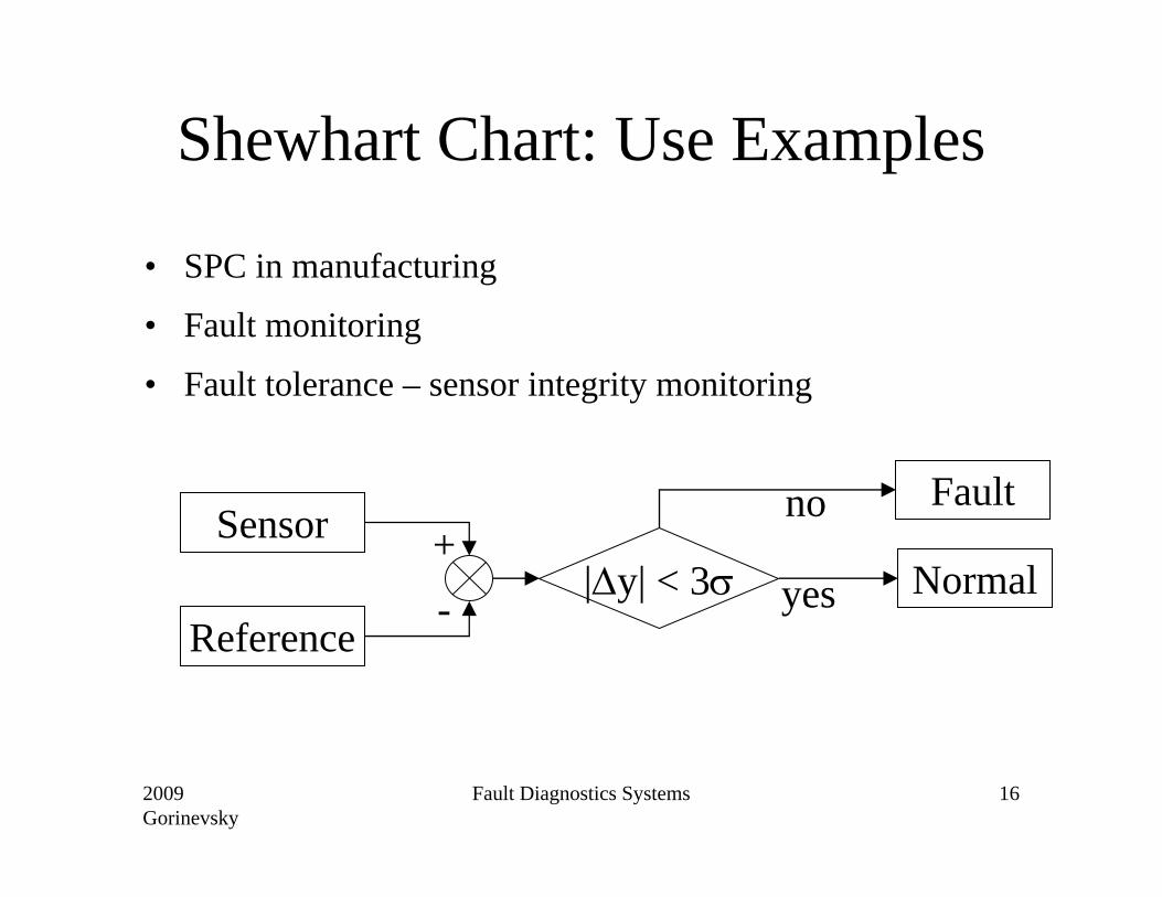
Shewhart Chart: Use Examples
• SPC in manufacturing
• Fault monitoring
• Fault tolerance – sensor integrity monitoring
Sensor
Reference-+
Fault
|∆y| < 3σ Normalyes
no

2009Gorinevsky
Fault Diagnostics Systems 17
Diagnostics Methods Overview
• Shewhart chart (Control chart)• Multivariable SPC, T2
• Model-based estimation – Least squares estimation
• Integrated diagnostics – Cascaded design

2009Gorinevsky
Fault Diagnostics Systems 18
Multivariable SPC• Univariate process
• Two independent univariate processes
( ))(1)(
)1,(1 222
cccFczP
Φ−+−Φ=−=>
( ) ( ) 22
222 ~22
2
22
21
1
11 χσµ
σµ
321321z
y
z
yz −− +=
22
02 ~ χσµ
⎟⎠⎞
⎜⎝⎛ −
=yz
( ) )2;(1 222 cFczP −=>
Chi-squared CDF
2009Gorinevsky
Fault Diagnostics Systems 19
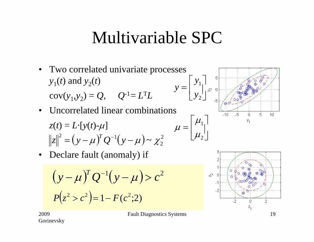
Multivariable SPC
• Two correlated univariate processes y1(t) and y2(t) cov(y1,y2) = Q, Q-1= LTL
• Uncorrelated linear combinationsz(t) = L·[y(t)-µ]
• Declare fault (anomaly) if ( ) ( ) 2
212 ~ χµµ −−= − yQyz T
⎥⎦
⎤⎢⎣
⎡=
2
1
yy
y
⎥⎦
⎤⎢⎣
⎡=
2
1
µµ
µ
( ) )2;(1 222 cFczP −=>
( ) ( ) 21 cyQy T >−− − µµ
2009Gorinevsky
Fault Diagnostics Systems 20
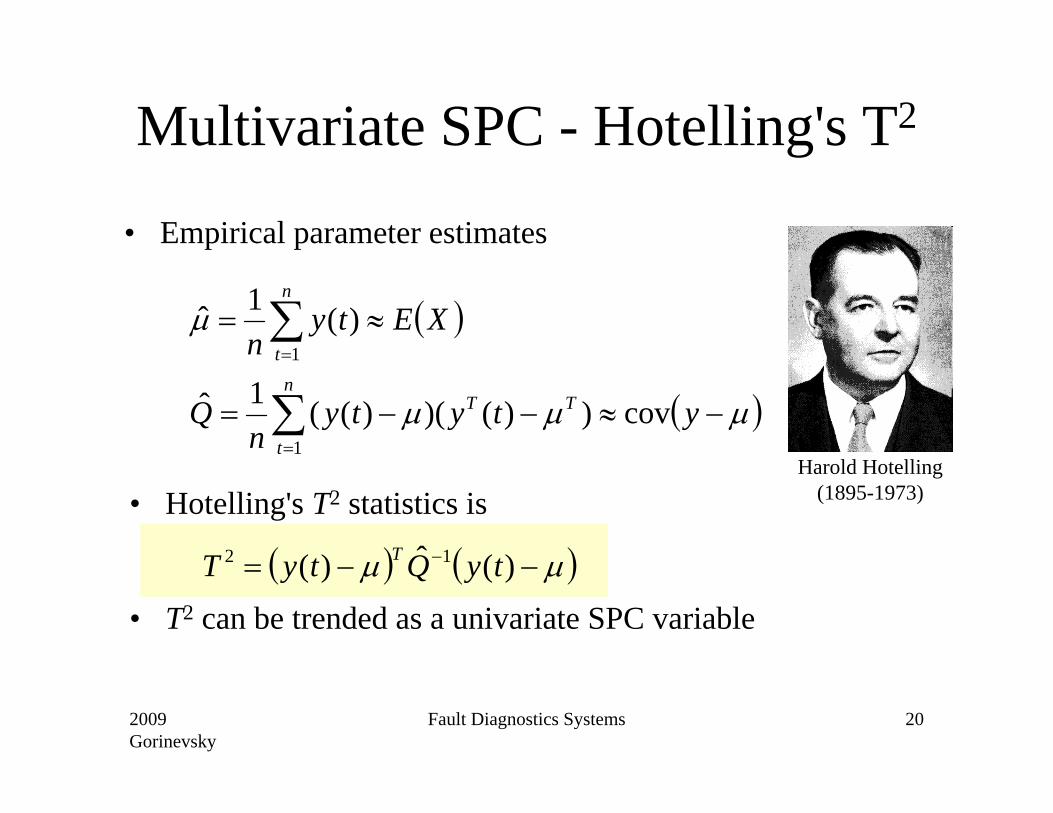
Multivariate SPC - Hotelling's T2
• Empirical parameter estimates
( )
( )µµµ
µ
−≈−−=
≈=
∑
∑
=
=
ytytyn
Q
XEtyn
Tn
t
T
n
t
cov))()()((1ˆ
)(1ˆ
1
1
• Hotelling's T2 statistics is
• T2 can be trended as a univariate SPC variable
( ) ( )µµ −−= − )(ˆ)( 12 tyQtyT T
Harold Hotelling(1895-1973)
2009Gorinevsky
Fault Diagnostics Systems 21
Diagnostics Methods Overview
• Shewhart chart (Control chart)• Multivariable SPC, T2
• Model-based estimation – Least squares estimation
• Integrated diagnostics – Cascaded design
2009Gorinevsky
Fault Diagnostics Systems 22
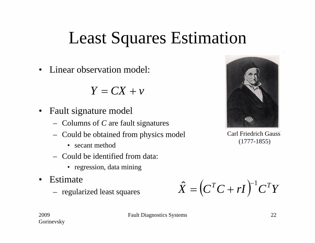
Least Squares Estimation
• Linear observation model:
• Fault signature model– Columns of C are fault signatures– Could be obtained from physics model
• secant method– Could be identified from data:
• regression, data mining
• Estimate – regularized least squares
vCXY +=
( ) YCrICCX TT 1ˆ −+=
Carl Friedrich Gauss (1777-1855)

2009Gorinevsky
Fault Diagnostics Systems 23
Bayesian Estimation
• Observation model: P(Y|X)
• Prior models: P(X)
• MAP estimate:
vCXY +=
( ) YCQRCQCX TT 1111ˆ −−−− +=
),0(~ QNv
),0(~ RNX
3214434421)(log
221
)|(log
221
11minargˆ
XP
R
XYP
QXCXYX
−−
−− +−=
...)(log 121 +=− − XRXXP T

2009Gorinevsky
Fault Diagnostics Systems 24
Model-based Residuals
Plant Model
input variables
Fault Diagnostics
prediction residual
+-
output variables
Plant Data Collected on-line
Input data
Output data
• Compute model-based prediction residualY = Yraw - f(U,X)
• If X = 0 (nominal case) we should have Y = 0. • Residuals Y reflect faults
– Sensor fault model - additive output change– Actuator fault model - additive input change

2009Gorinevsky
Fault Diagnostics Systems 25
Example: Jet Engine Model
• Nonlinear jet engine model– static map
• Residuals
• Linearized model
vCXY += ⎥⎦
⎤⎢⎣
⎡=
driftsensor EGTleak band Bleed
iondeteriorat TurbineX
),( XUfYY raw −=
XXUfC
∂∂
−=),(

2009Gorinevsky
Fault Diagnostics Systems 26
Example: Fault Estimates• Maintenance decision support tool
HoneywellLF507 EngineFleet
Estimates of (fault)performance parameter deterioration
1550 1600 1650 1700 1750 1800 1850 1900-1
-0.50
0.51
1.52
2.53
HP
Spo
ol D
eter
iora
tion
(%)
Sample No.
1550 1600 1650 1700 1750 1800 1850 1900-10-505
1015202530
Ble
ed B
and
Leak
age
(%)
Sample No.
1550 1600 1650 1700 1750 1800 1850 1900-40
-20
0
20
40
60
EG
T S
enso
r Offs
et (d
eg C
)
Sample No.
6-10-03
Ganguli, Deo, & Gorinevsky, IEEE CCA’04

2009Gorinevsky
Fault Diagnostics Systems 27
Diagnostics Methods Overview
• Shewhart chart (Control chart)• Multivariable SPC, T2
• Model-based estimation – Least squares estimation
• Integrated diagnostics – Cascaded design
2009Gorinevsky
Fault Diagnostics Systems 28
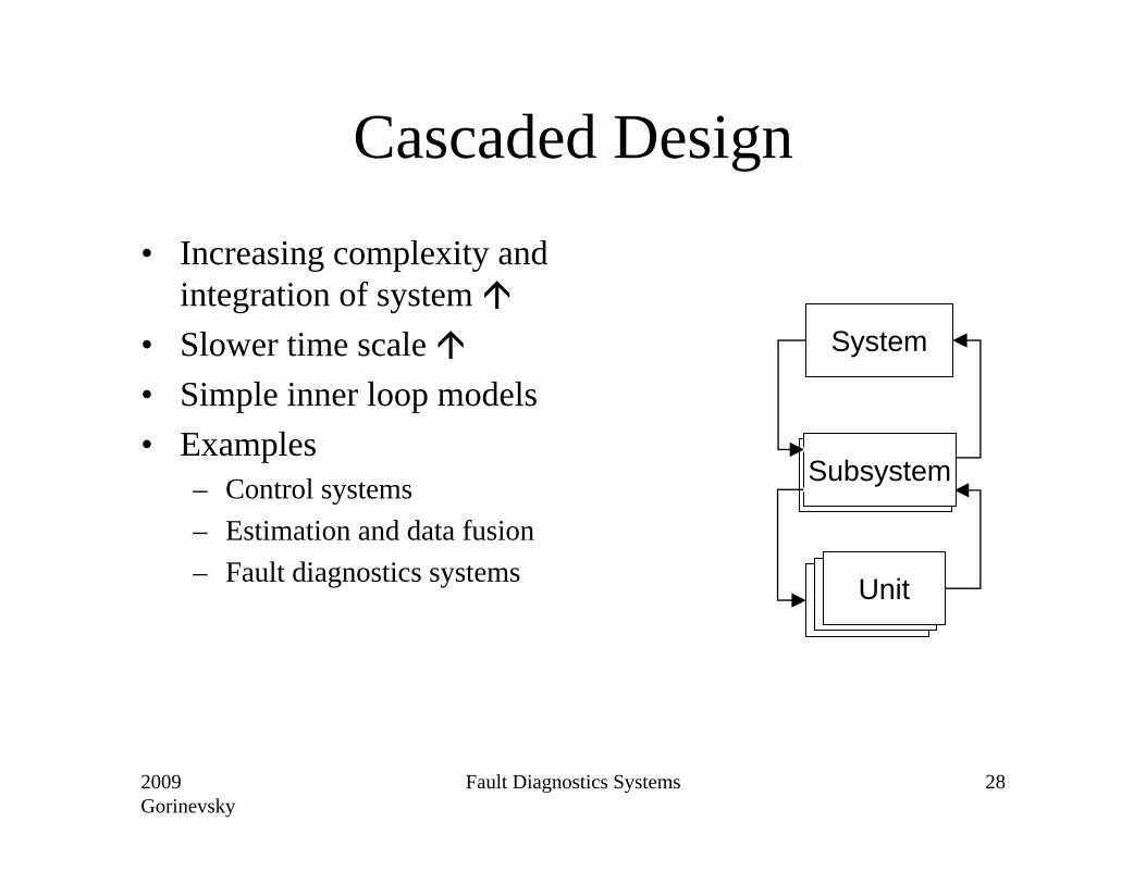
Cascaded Design
• Increasing complexity and integration of system
• Slower time scale • Simple inner loop models• Examples
– Control systems – Estimation and data fusion – Fault diagnostics systems
Unit
Subsystem
System
UnitUnit

2009Gorinevsky
Fault Diagnostics Systems 29
Integrated System Diagnostics• Complex integrated systems • Examples
– Aerospace vehicle, e.g. B777– Large scale computer network– Medical equipment
Subsystem 1 Diagnostics
Subsystem nDiagnostics
Integrated Diagnostic System
Decision Support Interface
Subsystem 2 Diagnostics …

2009Gorinevsky
Fault Diagnostics Systems 30
Discrete Fault Signatures
0000000
#0Null
001011#7011000#6010001#5000001#4100101#3010110#2100110#1
#6#5#4#3#2#1Root Cause Symptom Code
kk BY =Model of root cause fault k :
2009Gorinevsky
Fault Diagnostics Systems 31
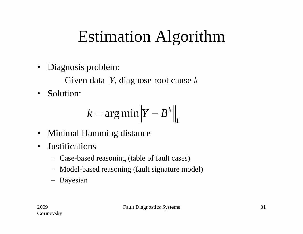
Estimation Algorithm
• Diagnosis problem:Given data Y, diagnose root cause k
• Solution:
• Minimal Hamming distance• Justifications
– Case-based reasoning (table of fault cases)– Model-based reasoning (fault signature model)– Bayesian
1minarg kBYk −=
2009Gorinevsky
Fault Diagnostics Systems 32
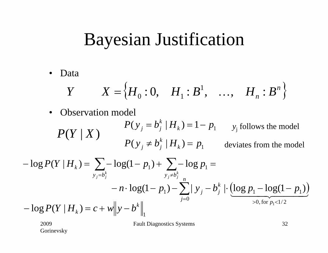
Bayesian Justification
• Data
• Observation model
{ }nn BHBHHXY :,,:,0: 1
10 K=
11)|( pHbyP kkjj −==
)|( XYP1)|( pHbyP k
kjj =≠
( )444 3444 21
2/1for ,0
110
1
1
)1log(log||)1log(<>=
−−⋅−−−⋅− ∑p
n
j
kjj ppbypn
1)|(log k
k bywcHYP −+=−
yj follows the model
deviates from the model
=−+−−=− ∑∑≠= k
jjkjj byby
k ppHYP 11 log)1log()|(log
2009Gorinevsky
Fault Diagnostics Systems 33
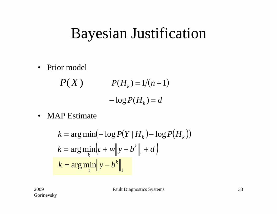
Bayesian Justification
• Prior model
• MAP Estimate
)(XP ( )11)( += nHP k
( )dbywck k
k+−+=
1minarg
dHP k =− )(log
( ) ( )( )kk HPHYPk log|logminarg −−=
1minarg k
kbyk −=

2009Gorinevsky
Fault Diagnostics Systems 34
Conclusions
• Basic diagnostics estimation methods – Are known for long time – Used in on-line systems for less time– Can be explained in several ways, e.g., Bayesian
• Engineering of fault diagnostics systems– Is new and current – Will be discussed in guest lectures– Not just diagnostics algorithms
2009Gorinevsky
Fault Diagnostics Systems 35
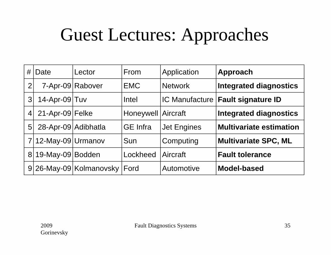
Guest Lectures: Approaches
Automotive
Aircraft
Computing
Jet Engines
Aircraft
IC Manufacture
Network
Application
Model-basedFordKolmanovsky26-May-099
Fault toleranceLockheedBodden19-May-098
Multivariate SPC, MLSunUrmanov12-May-097
Multivariate estimationGE InfraAdibhatla28-Apr-095
Integrated diagnostics HoneywellFelke21-Apr-094
Fault signature IDIntelTuv14-Apr-093
Integrated diagnostics EMCRabover7-Apr-092
ApproachFrom LectorDate#