EE16.468/16.568Lecture 2 Discrete optics: Mirrors, lens, mechanical mounts bulky labor intensive...
37
EE16.468/16.568 Lecture 2 Discrete optics: Mirrors, lens, mechanical mounts bulky labor intensive alignment ray optics environment sensitive Discrete optics v.s. Integrated optics Integrated optics: • Waveguide • Bendable, portable • Free-of-alignment • wave optics • robust • more functionalities
-
Upload
arleen-nicholson -
Category
Documents
-
view
221 -
download
0
Transcript of EE16.468/16.568Lecture 2 Discrete optics: Mirrors, lens, mechanical mounts bulky labor intensive...

EE16.468/16.568 Lecture 2
Discrete optics:
• Mirrors, lens, mechanical mounts• bulky• labor intensive alignment• ray optics • environment sensitive
Discrete optics v.s. Integrated optics
Integrated optics:
• Waveguide• Bendable, portable • Free-of-alignment• wave optics • robust• more functionalities

EE16.468/16.568 Lecture 2Discrete optics v.s. Integrated optics
Applications of Integrated optics:
• Transmitters and receivers, transceivers• All optical signal processing• Ultra-high speed communications (100Gbit/s), optical packet switching • RF spectrum analyzer• Smart sensors
Optical transceivers
OEIC, bio/sensor

EE16.468/16.568 Lecture 2Optical waveguides
2-D Optical waveguide
n2 < n1
Core, refractive index n1
Cladding, n2
Cladding, n2
y
x
z
d
0
1
90º-1
n0*sin(0) = n1*sin(1)
n1
n2
n0 = 1
Critical angle
n1*sin(90º-1)=n2*sin(90º)
Numerical aperture (NA)
cos(1)=n2/n1

EE16.468/16.568 Lecture 2Optical waveguides
2-D Optical waveguide
),90sin(sin 01max0 cnn
,sin1
2
n
nc
,)(
sin0
2/122
21
max n
nn
,)(sin 2/122
21max0 nnnNA
max2 : total acceptance angle

EE16.468/16.568 Lecture 2Optical waveguides
Example 2:
Calculate the acceptance angle of a core layer with index of n1= 1.468, and cladding layer of n0 = 1.447 for wavelength of 1.3m and 1.55 m.
Solution:
,)(
sin0
2/122
21
max n
nn
,7.9)(
sin 0
0
2/122
211
max
n
nn
acceptance angle: ,4.192 0max Wavelength independent:

EE16.468/16.568 Lecture 2
Fresnel equations
Reflections at the interface
n1
n2
n2 < n1
1
zy
x
1
2
s-polarized beam (senkrecht: perpendicular)
Trans-electric beam (TE)
n1
n2
1 1
2
zy
p-polarized beam (parallel)
Trans-magnetic beam (TM)
sss EtE 12
E1s E3s
E2s
sss ErE 13
2211
2211
coscos
coscos
nn
nnrs
ss rt 1
ppp EtE 12 ppp ErE 13
2112
2112
coscos
coscos
nn
nnrp
)1(2
1pp r
n
nt

EE16.468/16.568 Lecture 2
Fresnel equations
Reflections at the interface
n1
n2
n2 < n1
1
zy
x
1
2
n1
n2
1 1
2
zyE1s E3s
E2s
2
1
3
s
ss E
ER
2
1
2
1
2
s
ss E
E
n
nT
2
1
3
p
pp E
ER
2
1
2
1
2
p
pp E
E
n
nT
Poynting vector, energy flow rate
HES
HiE
HiaiknE
ˆ2
EnS

EE16.468/16.568 Lecture 2
Phase shift of reflection
Reflections at the interface
n2 < n1
2211
2211
coscos
coscos
nn
nnrs
2/11
221
2222 )sin(cos nnn
2211 sinsin nn
when 122
122 sin nn
1
21sin
n
ni.e. csin
0coscos 2211 nn because 0)cos()cos( 22
21
222
211 nnnn
In this case, 0sr is a real number
The reflection is not associated with phase shift, or phase shift is 0
n1
n2
1
zy
x
1
2
E1s E3s
E2s

EE16.468/16.568 Lecture 2
Phase shift of reflection
Reflections at the interface
n2 < n1
2211
2211
coscos
coscos
nn
nnrs
2/11
221
2222 )sin(cos nnn
when 122
122 sin nn
1
21sin
n
ni.e. csin
n1
n2
1zy
x
1
2
E1s E3s
E2s
2/1221
22111
2/1221
22111
)sin(cos
)sin(cos
nnin
nninrs
1
2/121
2
1
2/121
221
2
cos
)sin(sin
cos
)/(sin
2tan
cnn
0
30
60
90
120
150
180
0 10 20 30 40 50 60 70 80 90
c
1

EE16.468/16.568 Lecture 2
Evanescent wave
Reflections at the interface
n2 < n1
n1
n2
1
zy
x
1
2
E1s E3s
E2s
)(222
222 )0()0( zkxkis
rkiss
zxeEeEE
Momentum conservation
zz kk 12 2211 sin2
sin2
nn
2
2/1
12
22
2122/1
122
122
2/122
222 1sin
2sin
2
in
nninnkkk zx
zikdxs
zikxss
zz eeEeeEE 222 /222 )0()0(
Attenuated wave, penetration depth: d
12/1
12
22
2121
2 1sin2
n
nnd

EE16.468/16.568 Lecture 2
Optical modes
k*n1*AC – k*n1*AB = 2m
AC = AB*cos(21) AB = d/sin(1)
1 2
A
B
C
1
1
1
d
md
knd
kn 2sin
)2cos(sin 1
111
1
m
ddkn 2
sinsin
sincos
11
12
12
1
mdkn 2
sin
1sincos
1
12
12
1
mdkn 2
sin
1sinsin1
1
12
12
1
mdkn 2sin
sin2
1
12
1
mdkn 2sin2 11
Ray optics approach
dmn mm 2
sinsin ,0,11
2/1
20
201
2/1
,12
01,101
)2
()(
)sin1(cos
dmkkn
knkn mmm

EE16.468/16.568 Lecture 2
Optical modes
1 2
A
B
C
1
1
1
d
Ray optics approach
Propagation constant
20
201
2 )2
()(d
mkknm
Effective index: effm nk0

EE16.468/16.568 Lecture 2
Optical modes, considering phase shift at reflection
k*n1*AC – k*n1*AB + 2* = 2m
AC = AB*cos(21) AB = d/sin(1)
1 2
A
B
C
1
1
1
d
md
knd
kn 22sin
)2cos(sin 1
111
1
m
ddkn 22
sinsin
sincos
11
12
12
1
mdkn 22
sin
1sincos
1
12
12
1
mdkn 22
sin
1sinsin1
1
12
12
1
mdkn 22sin
sin2
1
12
1
2tan)
2sin
2tan( 11
md
kn
Ray optics approach
2
2/122
2
11 cos
)sin(sin)
2sin
2tan(
cm
dkn

EE16.468/16.568 Lecture 2
Optical modes
1 2
A
B
C
1
1
1
d
Ray optics approach
Cut-off wavelength :
,/])(2
[ 2/122
21
nnd
m
c
V number, normalized thickness, or normalized frequency
,)(2/2 2/12
221 nn
dV
,/]2[ Vm
,2
)( cV
mdkn 22sin2 11 21
22
21 1cossinn
n

EE16.468/16.568 Lecture 2
Optical modes
Ray optics approach
Example: estimate the number of modes
• waveguide thickness 100m, free-space wavelength 1m,
,490.11 n
49 modes
,4.76)(2 2/12
221 nn
aV
,7.48/]2[ Vm
,470.12 n
,/])(2
[ 2/122
21
nnd
m

EE16.468/16.568 Lecture 2Ray optics approach
1
2/121
2
11 sin
)sin(cos)
2sin
2tan(
cm
dkn
Normalized waveguide equation:
,1
tan2
)1( 1
b
bmbV
,cos
22
21
221
221
22
21
22
2
nn
nn
nn
nnb eff
,01
tan2
)1(),,( 1
b
bmbVbmVf
b: normalized propagation constant,cos1 meff nn
,)(2/2 2/12
221 nn
dV

EE16.468/16.568 Lecture 2Ray optics approach
Discussion:
,cos
22
21
221
221
22
21
22
2
nn
nn
nn
nnb eff
,cos1 meff nn
Attenuated wave, penetration depth: D
1
2/122
21
12/1
222
2121
2
)2
1sin2
bnn
n
nnD
,cos)( 221
221
22
21 nnbnn

EE16.468/16.568 Lecture 2Ray optics approach
Discussions:
• mode numbers v.s. index difference and wavelength• effective index difference of higher and lower order modes• mode profiles dependence on index difference and wavelength
Example 1:
Calculate the thickness of a core layer with index of n1= 1.468, and cladding layer of n0 = 1.447 for wavelength of 1.3m.
Solution:
,2
)(2 2/12
221
nna
V,/]2[ Vm ,0,1 m For single mode:
0.3
0.4
0.5
0.6
0.7
0.8
0.5 0.7 0.9 1.1 1.3 1.5 1.7 1.9
thickness
pi

EE16.468/16.568 Lecture 2Ray optics approach
m
cmm m
dkn
sin
)sin(cos)
2sin
2tan(
2/122
1
Normalized waveguide equation:
,1
)2
)1(tan(b
bmbV
,cos1 meff nn
-4
-2
0
2
4
0 0.2 0.4 0.6 0.8 1
m=0m=1(b/(1-b)) .̂5
b
V = 3.3

EE16.468/16.568 Lecture 2Ray optics approach
Asymmetric waveguide
),1
(tan)1
(tan2
)1( 11
b
b
b
bmbV
n1
n2
n0 = 1
n3
23
21
22
23
nn
nn

EE16.468/16.568 Lecture 2Wave optics approach
0
Dielectric materials
Maxwell equations:
t
BE
D
t
DJH
0 B
ED
0J HB
t
BE
0 D
t
DH
0 B
Maxwell equations in dielectric materials:
BjE
0 D
DjH
0 B
phasor
)()( BjE
EEE
22)(

EE16.468/16.568 Lecture 2Wave optics approach
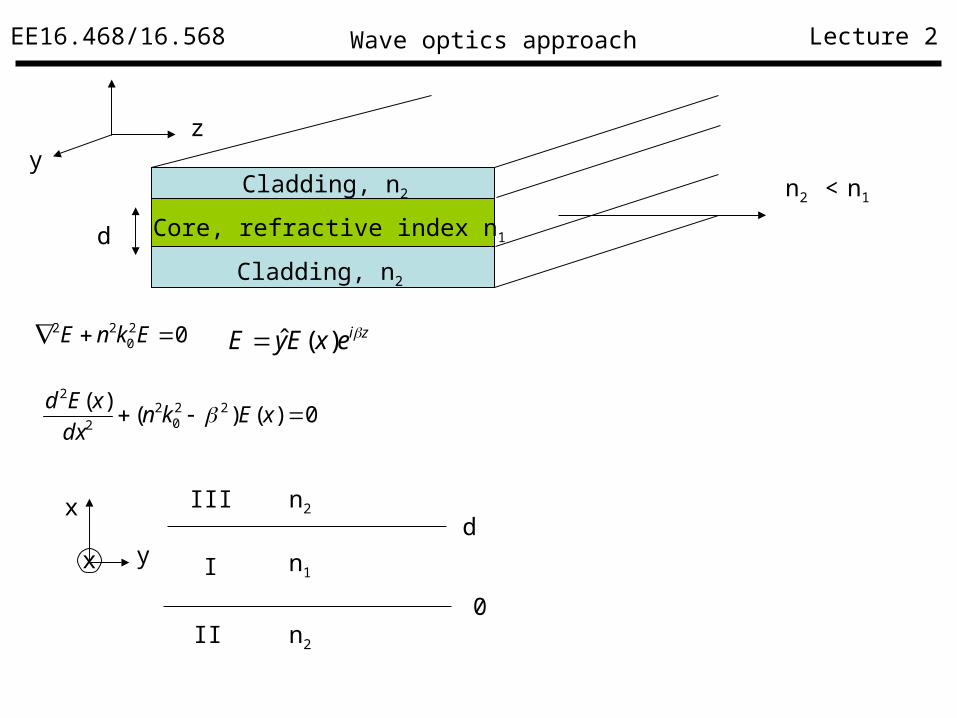
2-D Optical waveguide
n2 < n1
Core, refractive index n1
Cladding, n2
Cladding, n2
y
x
z
d
)(ˆ xEyE
TE mode:
022 EE
Helmholtz Equation:
022 EkE
22 k
)(ˆ xHyH TM mode:
Free-space solutions
ikzeEyE 0ˆ
ikzeExE 0ˆ
EE16.468/16.568 Lecture 2Wave optics approach
ziexEyE )(ˆ
020
22 EknE
n2 < n1
Core, refractive index n1
Cladding, n2
Cladding, n2
yz
d
I
II
III
yx
xd
0
n1
n2
n2
0)()()( 22
02
2
2
xEkndx
xEd
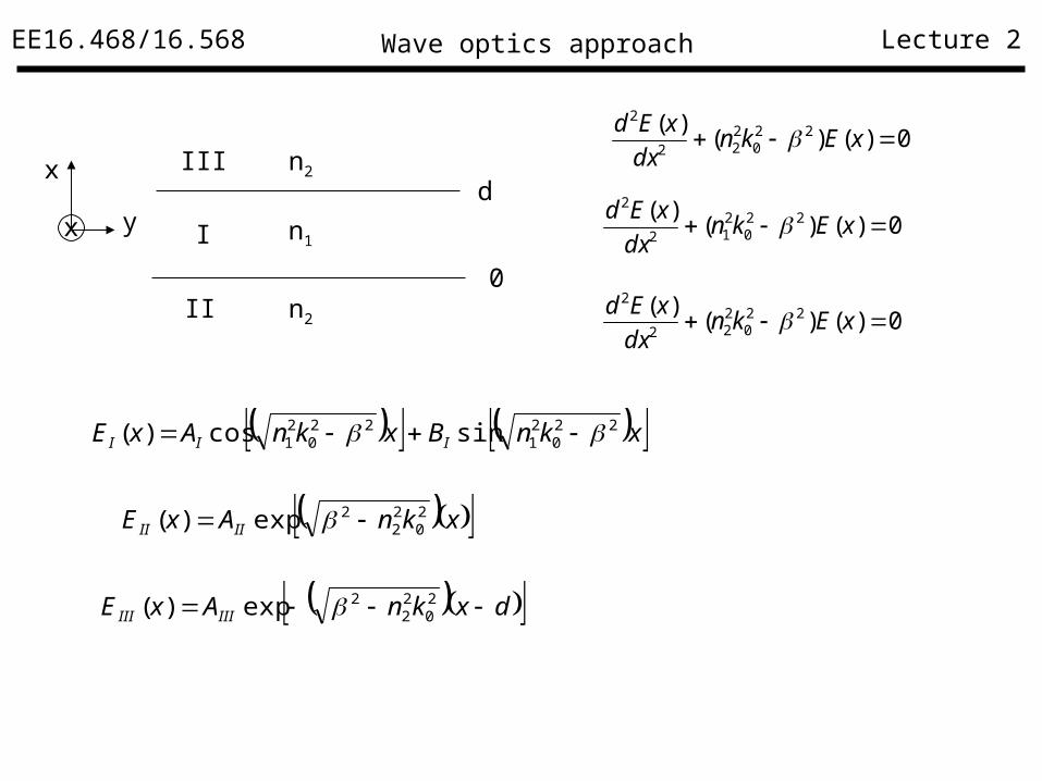
EE16.468/16.568 Lecture 2Wave optics approach
I
II
III
yx
xd
0
n1
n2
n2
0)()()( 22
0212
2
xEkndx
xEd
0)()()( 22
0222
2
xEkndx
xEd
0)()()( 22
0222
2
xEkndx
xEd
xknBxknAxE III22
021
220
21 sincos)(
xknAxE IIII20
22
2exp)(
dxknAxE IIIIII 20
22
2exp)(

EE16.468/16.568 Lecture 2Wave optics approach
I
II
III
yx
x
n1
n2
n2
0)()()( 22
0212
2
xEkndx
xEd
0)()()( 22
0222
2
xEkndx
xEd
0)()()( 22
0222
2
xEkndx
xEd
xknBxknAxE III22
021
220
21 sincos)(
2/exp)( 20
22
2 dxknAxE IIII
2/exp)( 20
22
2 dxknAxE IIIIII
d
0

EE16.468/16.568 Lecture 2Wave optics approach
I
II
III
yx
x
n1
n2
n2
0sin0cos)( 220
21
220
21 knBknAxE III
0exp)( 20
22
2 knAxE IIII
0|)()( xIII xExE
III AA
dxIIII xExE |)()(
dxIIII xEdx
dxE
dx
d |)()(
0|)()( xIII xExE
0|)()( xIII xEdx
dxE
dx
d
d
0

EE16.468/16.568 Lecture 2Wave optics approach
I
II
III
yx
x
n1
n2
n2
0cos0sin 220
21
220
21
220
21
220
21
20
22
2 knknBknAknknA IIII
0|)()( xIII xEdx
dxE
dx
d
22
021
20
22
2
kn
knAB III
dxIIII xExE |)()(
dxIIII xEdx
dxE
dx
d |)()(
0|)()( xIII xExE
0|)()( xIII xEdx
dxE
dx
d
d
0

EE16.468/16.568 Lecture 2Wave optics approach
I
II
III
yx
x
n1
n2
n2
dknknBdknAknknA IIIII22
021
220
21
220
21
220
21
20
22
2 cossin
dknBdknAA IIIII22
021
220
21 sincos
dknBdknA
dknBdknA
kn
kn
II
II
220
21
220
21
220
21
220
21
20
22
2
220
21
cossin
sincos
dxIIII xExE |)()(
dxIIII xEdx
dxE
dx
d |)()(
0|)()( xIII xExE
0|)()( xIII xEdx
dxE
dx
d
d
0
22
021
20
22
2
kn
knAB III

EE16.468/16.568 Lecture 2Wave optics approach
dknBdknA
dknBdknA
kn
kn
II
II
220
21
220
21
220
21
220
21
20
22
2
220
21
cossin
sincos
22
021
20
22
2
kn
knAB II
dkn
kn
kndkn
dknkn
kndkn
kn
kn
220
2122
021
20
22
222
021
220
2122
021
20
22
222
021
20
22
2
220
21
cossin
sincos
220
21 knh
qhdh
hdqh
q
h
)tan(
)tan( 20
22
2 knq
)/1(
22)tan(
2222 hqh
q
qh
hqhd
Graphic solution

EE16.468/16.568 Lecture 2Dispersion
Dispersion
1
0|
d
d
d
dvg
v
ZieAA )()(
)(tA
))(()||)(())(()(
0000
)(
gv
ZtziZ
d
dtzitz
d
di
tzi eeeezA
Time delay )()(v
ZtAtA

EE16.468/16.568 Lecture 2Dispersion
• Material dispersion
,|0
d
dvg ,
gg v
L ,)()(
2
2
d
nd
cd
d
Lg
),(2
2
d
nd
cDm , LDmg
Example --- material dispersion
Calculate the material dispersion effect for LED with line width of 100nm and a laser with a line width of 2nm for a fiber with dispersion coefficient of Dm = 22pskm-1nm-1 at 1310nm.
,2.2 nsLDm
Solution:
,44psLDm
for the LED
for the Laser

EE16.468/16.568 Lecture 2
• Waveguide dispersion
,|0
d
dvg ,
gg v
L
,2)2(
984.1)(
22
2
2
cna
N
d
d
Lgg
, LDmg
Example --- waveguide dispersionn2 = 1.48, and delta n = 0.2 percent. Calculate Dw at 1310nm.
Solution:
,)()(
)(2
2212
dV
VbdV
c
nnn
d
d
Lg
,)()(
2
2212
dV
VbdV
c
nnnDw
,)/996.01428.1( 2Vb for V between 1.5 – 2.5.
,26.0)(
2
2
dV
VbdV
),/(9.1)()(
2
2212 kmnmps
dV
VbdV
c
nnnDw
Dispersion

EE16.468/16.568 Lecture 2
• Waveguide mode dispersion
Dispersion
n1
n2
n0 = 1
n3
Higher order mode, 2
~|0 n
c
d
dvg
Lower order mode, 1
~|0 n
c
d
dvg
)/(112 n
c
n
c
Lg
EE16.468/16.568 Lecture 2Dispersion
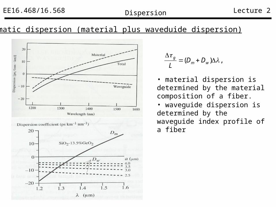
• chromatic dispersion (material plus waveduide dispersion)
,)(
wmg DD
L
• material dispersion is determined by the material composition of a fiber.
• waveguide dispersion is determined by the waveguide index profile of a fiber

EE16.468/16.568 Lecture 2
• Dispersion induced limitations
,2
1
2/1B
• For RZ bit With no intersymbol interference
,1
2/1B
• For NRZ bit With no intersymbol interference
Dispersion

EE16.468/16.568 Lecture 2
Dispersion induced limitations
,2
1
2/1B
• Optical and Electrical Bandwidth
,7.03 Bf dB
• Bandwidth length product
,25.0
D
BL
Dispersion

EE16.468/16.568 Lecture 2
Dispersion induced limitations
,16/ 12/1
pskmDL
,8.27.03 GHzBf dB
,9.3625.0 1kmGbs
DBL
Example --- bit rate and bandwidth
Calculate the bandwidth and length product for an optical fiber with chromatic dispersion coefficient 8pskm-1nm-1 and optical bandwidth for 10km of this kind of fiber and linewidth of 2nm.
Solution:
• Fiber limiting factor absorption or dispersion?
,5.21025.0 dBkmdBLoss
Dispersion