EE123 Digital Signal Processing - University of …ee123/sp16/Notes/Lecture09_Spect... · M....
34
M. Lustig, EECS UC Berkeley EE123 Digital Signal Processing Lecture 9 Spectral Analysis using DFT based on slides by J.M. Kahn
-
Upload
nguyenhuong -
Category
Documents
-
view
236 -
download
0
Transcript of EE123 Digital Signal Processing - University of …ee123/sp16/Notes/Lecture09_Spect... · M....
M. Lustig, EECS UC Berkeley
EE123Digital Signal Processing
Lecture 9Spectral Analysis using DFT
based on slides by J.M. Kahn

M. Lustig, EECS UC Berkeley
Demo
• iSpectrum Demo
M. Lustig, EECS UC Berkeley
Announcements
• Last time: – FFT
• Today:– Frequency analysis with DFT– Windowing– Effect of zero-padding
M. Lustig, EECS UC Berkeley
Spectral analysis using the DFT
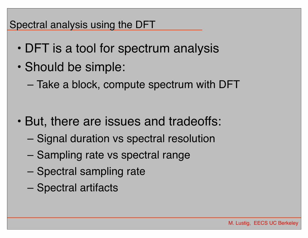
• DFT is a tool for spectrum analysis• Should be simple:
– Take a block, compute spectrum with DFT
• But, there are issues and tradeoffs:– Signal duration vs spectral resolution– Sampling rate vs spectral range– Spectral sampling rate– Spectral artifacts
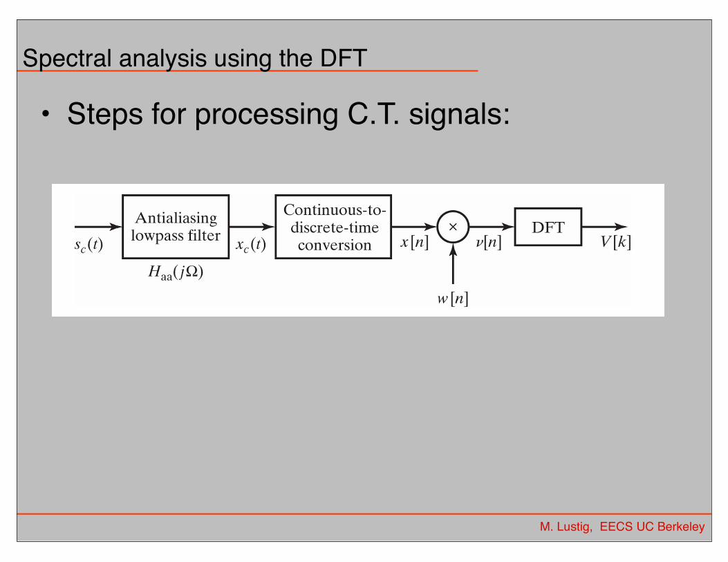
• Steps for processing C.T. signals:
Spectral Analysis with the DFT
Consider these steps of processing continuous-time signals:
Miki Lustig UCB. Based on Course Notes by J.M Kahn Spring 2014, EE123 Digital Signal Processing
M. Lustig, EECS UC Berkeley
Spectral analysis using the DFT

• Two important tools:– Applying a window - reduced artifacts– Zero-padding - increases spectral sampling
Spectral Analysis with the DFT
Two important tools:
Applying a window to the input signal – reduces spectralartifactsPadding input signal with zeros – increases the spectralsampling
Key Parameters:
Parameter Symbol Units
Sampling interval T sSampling frequency ⌦
s
= 2⇡T
rad/sWindow length L unitlessWindow duration L · T sDFT length N � L unitlessDFT duration N · T s
Spectral resolution ⌦
s
L
= 2⇡L·T rad/s
Spectral sampling interval ⌦
s
N
= 2⇡N·T rad/s
Miki Lustig UCB. Based on Course Notes by J.M Kahn Spring 2014, EE123 Digital Signal Processing
M. Lustig, EECS UC Berkeley
Spectral analysis using the DFT
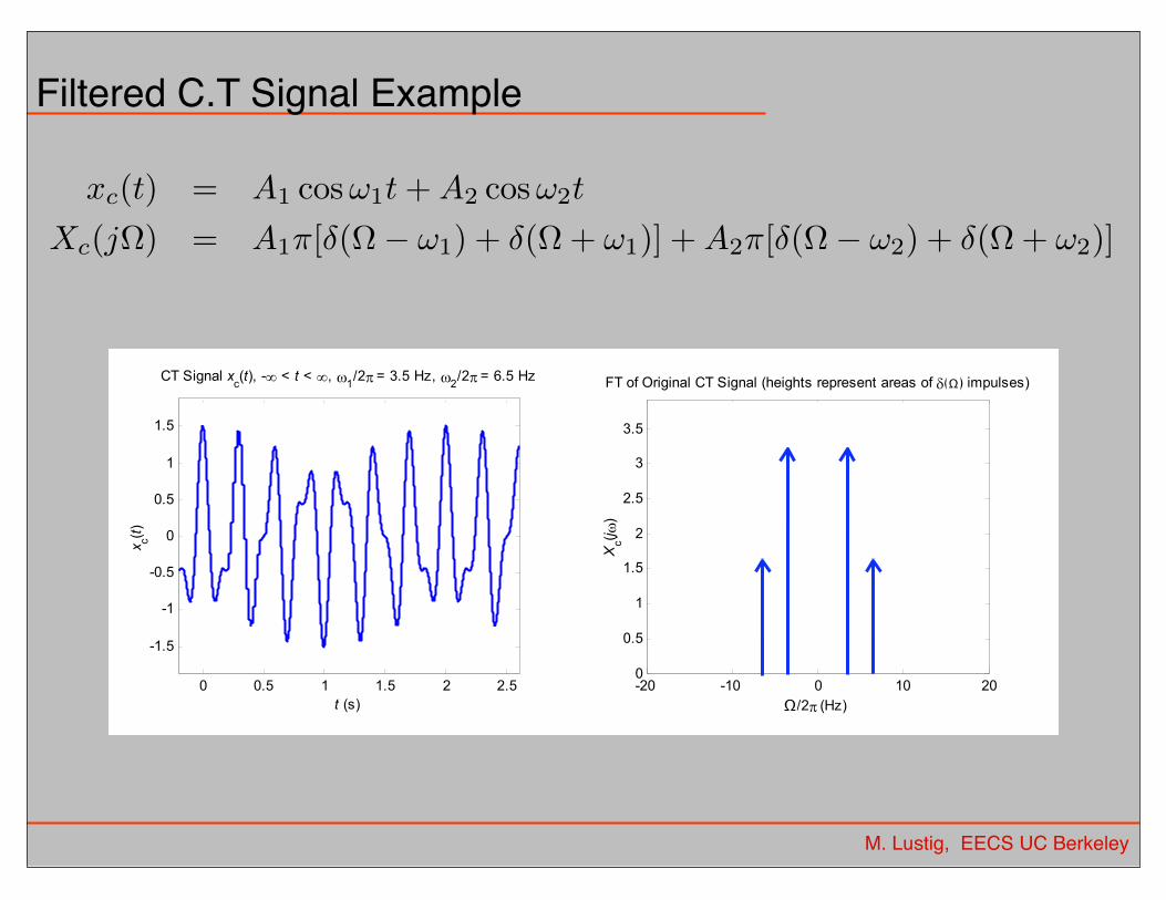
Filtered Continuous-Time Signal
We consider an example:
x
c
(t) = A
1
cos!1
t + A
2
cos!2
t
X
c
(j⌦) = A
1
⇡[�(⌦� !1
) + �(⌦+ !1
)] + A
2
⇡[�(⌦� !2
) + �(⌦+ !2
)]
0 0.5 1 1.5 2 2.5
-1.5
-1
-0.5
0
0.5
1
1.5
t (s)
x c(t
)
CT Signal xc(t), - < t < ,
1/2 = 3.5 Hz,
2/2 = 6.5 Hz
-20 -10 0 10 200
0.5
1
1.5
2
2.5
3
3.5
/2 (Hz)
Xc(j
)
FT of Original CT Signal (heights represent areas of ( ) impulses)
Miki Lustig UCB. Based on Course Notes by J.M Kahn Spring 2014, EE123 Digital Signal Processing
Ω
Ω
M. Lustig, EECS UC Berkeley
Filtered C.T Signal Example
xc(t) = A1 cos!1t+A2 cos!2t
Xc(j⌦) = A1⇡[�(⌦� !1) + �(⌦+ !1)] +A2⇡[�(⌦� !2) + �(⌦+ !2)]
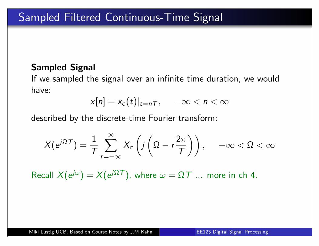
Sampled Filtered Continuous-Time Signal
Sampled SignalIf we sampled the signal over an infinite time duration, we wouldhave:
x [n] = x
c
(t)|t=nT
, �1 < n < 1
described by the discrete-time Fourier transform:
X (e j⌦T ) =1
T
1X
r=�1X
c
✓j
✓⌦� r
2⇡
T
◆◆, �1 < ⌦ < 1
Recall X (e j!) = X (e j⌦T ), where ! = ⌦T ... more in ch 4.
Miki Lustig UCB. Based on Course Notes by J.M Kahn Spring 2014, EE123 Digital Signal Processing
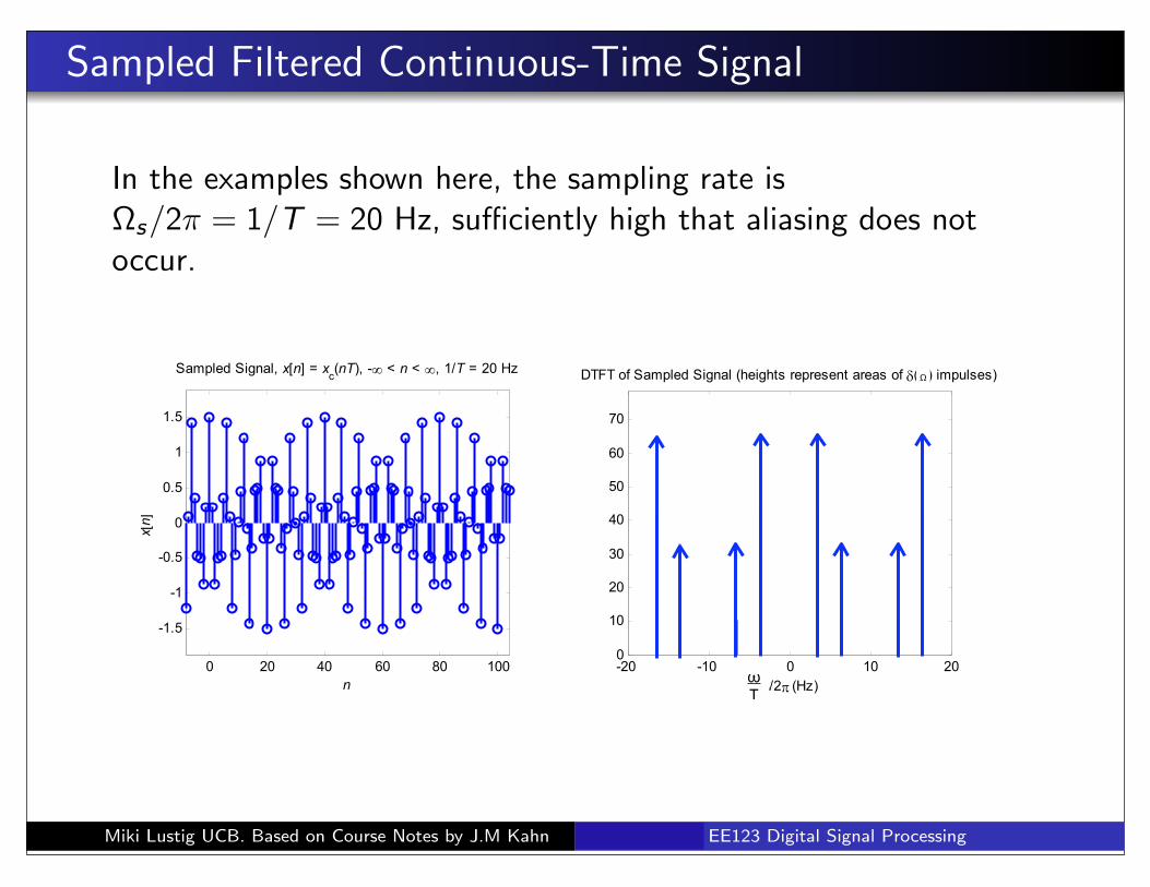
Sampled Filtered Continuous-Time Signal
In the examples shown here, the sampling rate is⌦s
/2⇡ = 1/T = 20 Hz, su�ciently high that aliasing does notoccur.
0 20 40 60 80 100
-1.5
-1
-0.5
0
0.5
1
1.5
n
x[n]
Sampled Signal, x[n] = xc(nT), - < n < , 1/T = 20 Hz
-20 -10 0 10 200
10
20
30
40
50
60
70
/2 (Hz)
X(ejT)
DTFT of Sampled Signal (heights represent areas of ( ) impulses)
Miki Lustig UCB. Based on Course Notes by J.M Kahn Spring 2014, EE123 Digital Signal Processing
ωT
Ω

Windowed Sampled Signal
Block of L Signal SamplesIn any real system, we sample only over a finite block of L samples:
x [n] = x
c
(t)|t=nT
, 0 n L� 1
This simply corresponds to a rectangular window of duration L.
Recall: in Homework 1 we explored the e↵ect of rectangularand triangular windowing
Miki Lustig UCB. Based on Course Notes by J.M Kahn Spring 2014, EE123 Digital Signal Processing
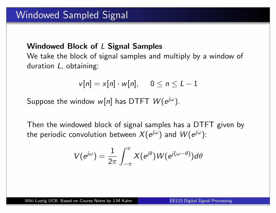
Windowed Sampled Signal
Windowed Block of L Signal SamplesWe take the block of signal samples and multiply by a window ofduration L, obtaining:
v [n] = x [n] · w [n], 0 n L� 1
Suppose the window w [n] has DTFT W (e j!).
Then the windowed block of signal samples has a DTFT given bythe periodic convolution between X (e j!) and W (e j!):
V (e j!) =1
2⇡
Z ⇡
�⇡X (e j✓)W (e j(!�✓))d✓
Miki Lustig UCB. Based on Course Notes by J.M Kahn Spring 2014, EE123 Digital Signal Processing
Windowed Sampled Signal
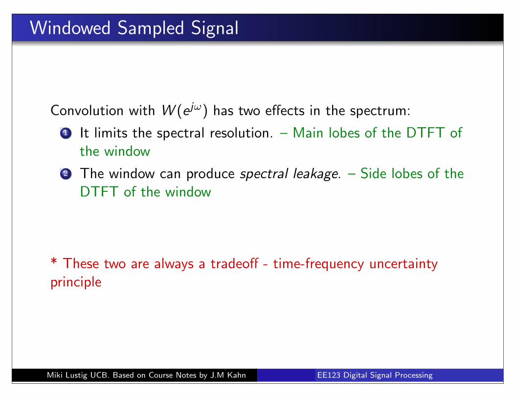
Convolution with W (e j!) has two e↵ects in the spectrum:
1 It limits the spectral resolution. – Main lobes of the DTFT ofthe window
2 The window can produce spectral leakage. – Side lobes of theDTFT of the window
* These two are always a tradeo↵ - time-frequency uncertaintyprinciple
Miki Lustig UCB. Based on Course Notes by J.M Kahn Spring 2014, EE123 Digital Signal Processing
Windows (as defined in MATLAB)
-5 0 50
0.2
0.4
0.6
0.8
1
n
w[n
]
boxcar(M+1), M = 8
-5 0 50
0.2
0.4
0.6
0.8
1
n
w[n
]
boxcar(M+1), M = 8
-5 0 50
0.2
0.4
0.6
0.8
1
n
w[n
]
triang(M+1), M = 8
-5 0 50
0.2
0.4
0.6
0.8
1
n
w[n
]
triang(M+1), M = 8
-5 0 50
0.2
0.4
0.6
0.8
1
n
w[n
]
bartlett(M+1), M = 8
-5 0 50
0.2
0.4
0.6
0.8
1
n
w[n
]
bartlett(M+1), M = 8
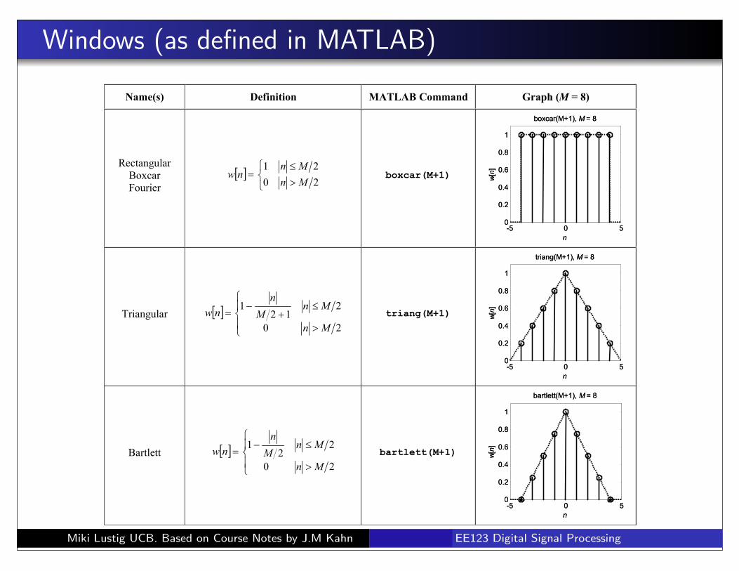
Name(s) Definition MATLAB Command Graph (M = 8)
Rectangular
Boxcar
Fourier
nw20
21
Mn
Mnboxcar(M+1)
Triangular nw
20
212
1
Mn
MnM
n
triang(M+1)
Bartlett nw
20
22
1
Mn
MnM
n
bartlett(M+1)
Miki Lustig UCB. Based on Course Notes by J.M Kahn Spring 2014, EE123 Digital Signal Processing

Windows (as defined in MATLAB)
-5 0 50
0.2
0.4
0.6
0.8
1
n
w[n
]
hann(M+1), M = 8
-5 0 50
0.2
0.4
0.6
0.8
1
n
w[n
]
hann(M+1), M = 8
-5 0 50
0.2
0.4
0.6
0.8
1
n
w[n
]
hanning(M+1), M = 8
-5 0 50
0.2
0.4
0.6
0.8
1
n
w[n
]
hanning(M+1), M = 8
-5 0 50
0.2
0.4
0.6
0.8
1
n
w[n
]
hamming(M+1), M = 8
-5 0 50
0.2
0.4
0.6
0.8
1
n
w[n
]
hamming(M+1), M = 8
Name(s) Definition MATLAB Command Graph (M = 8)
Hann nw
20
22
cos12
1
Mn
MnM
n
hann(M+1)
Hanning nw
20
212
cos12
1
Mn
MnM
n
hanning(M+1)
Hamming nw
20
22
cos46.054.0
Mn
MnM
n
hamming(M+1)
Miki Lustig UCB. Based on Course Notes by J.M Kahn Spring 2014, EE123 Digital Signal Processing
Windows
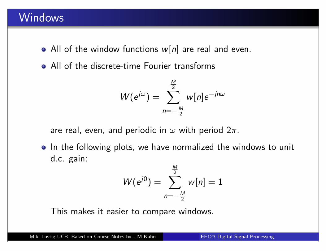
All of the window functions w [n] are real and even.
All of the discrete-time Fourier transforms
W (e j!) =
M
2X
n=�M
2
w [n]e�jn!
are real, even, and periodic in ! with period 2⇡.
In the following plots, we have normalized the windows to unitd.c. gain:
W (e j0) =
M
2X
n=�M
2
w [n] = 1
This makes it easier to compare windows.
Miki Lustig UCB. Based on Course Notes by J.M Kahn Spring 2014, EE123 Digital Signal Processing

Window Example
0 0.5 1 1.5 2 2.5 3
-0.2
0
0.2
0.4
0.6
0.8
1
W(ej
)
M = 16
Boxcar
Triangular
0 0.5 1 1.5 2 2.5 3
-0.2
0
0.2
0.4
0.6
0.8
1
W(ej
)
M = 16
Hanning
Hamming
0 0.5 1 1.5 2 2.5 3-70
-60
-50
-40
-30
-20
-10
0
20
lo
g1
0|W
(ej
)|
M = 16
Boxcar
Triangular
0 0.5 1 1.5 2 2.5 3-70
-60
-50
-40
-30
-20
-10
0
20
lo
g1
0|W
(ej
)|
M = 16
Hanning
Hamming
Miki Lustig UCB. Based on Course Notes by J.M Kahn Spring 2014, EE123 Digital Signal Processing
ωω
ω ω
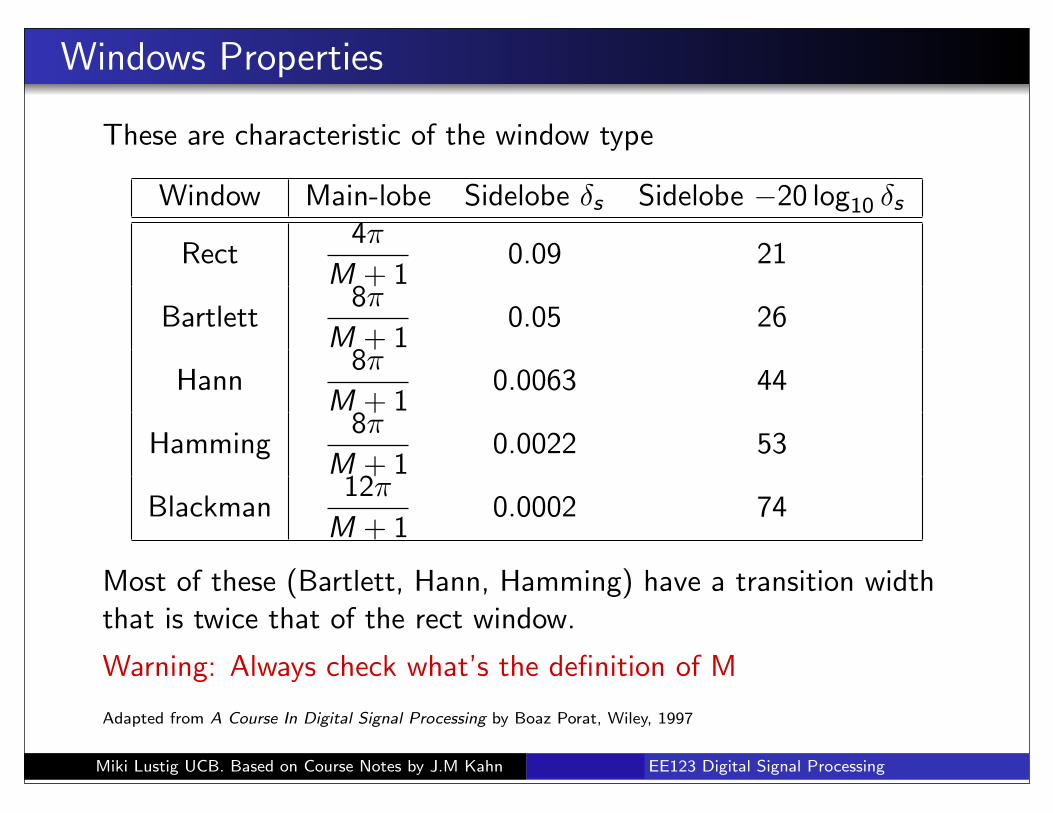
Windows Properties
These are characteristic of the window type
Window Main-lobe Sidelobe �s
Sidelobe �20 log10
�s
Rect4⇡
M + 10.09 21
Bartlett8⇡
M + 10.05 26
Hann8⇡
M + 10.0063 44
Hamming8⇡
M + 10.0022 53
Blackman12⇡
M + 10.0002 74
Most of these (Bartlett, Hann, Hamming) have a transition widththat is twice that of the rect window.
Warning: Always check what’s the definition of M
Adapted from A Course In Digital Signal Processing by Boaz Porat, Wiley, 1997
Miki Lustig UCB. Based on Course Notes by J.M Kahn Spring 2014, EE123 Digital Signal Processing

Windows Examples
Here we consider several examples. As before, the sampling rate is⌦s
/2⇡ = 1/T = 20 Hz.Rectangular Window, L = 32
0 5 10 15 20 25 300
0.2
0.4
0.6
0.8
1
1.2
n
w[n
]
Rectangular Window, L = 32
-20 -10 0 10 200
5
10
15
20
25
30
35
40
/2 (Hz)
|W(ejT)|
DTFT of Rectangular Window
0 5 10 15 20 25 30
-1.5
-1
-0.5
0
0.5
1
1.5
n
v[n]
Sampled, Windowed Signal, Rectangular Window, L = 32
-20 -10 0 10 200
5
10
15
20
/2 (Hz)
|V(ejT)|
DTFT of Sampled, Windowed Signal
Miki Lustig UCB. Based on Course Notes by J.M Kahn Spring 2014, EE123 Digital Signal Processing
Ω
ωT
ωT
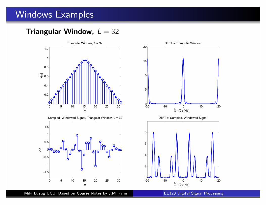
Windows Examples
Triangular Window, L = 32
0 5 10 15 20 25 300
0.2
0.4
0.6
0.8
1
1.2
n
w[n
]Triangular Window, L = 32
-20 -10 0 10 200
5
10
15
20
/2 (Hz)
|W(ejT)|
DTFT of Triangular Window
0 5 10 15 20 25 30
-1.5
-1
-0.5
0
0.5
1
1.5
n
v[n]
Sampled, Windowed Signal, Triangular Window, L = 32
-20 -10 0 10 200
2
4
6
8
/2 (Hz)
|V(ejT)|
DTFT of Sampled, Windowed Signal
Miki Lustig UCB. Based on Course Notes by J.M Kahn Spring 2014, EE123 Digital Signal Processing
ωT
ωT
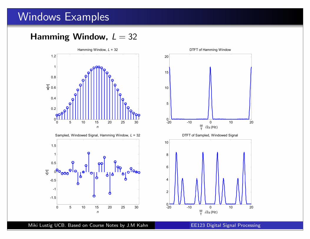
Windows Examples
Hamming Window, L = 32
0 5 10 15 20 25 300
0.2
0.4
0.6
0.8
1
1.2
n
w[n
]Hamming Window, L = 32
-20 -10 0 10 200
5
10
15
20
/2 (Hz)
|W(ejT)|
DTFT of Hamming Window
0 5 10 15 20 25 30
-1.5
-1
-0.5
0
0.5
1
1.5
n
v[n]
Sampled, Windowed Signal, Hamming Window, L = 32
-20 -10 0 10 200
2
4
6
8
10
/2 (Hz)
|V(ejT)|
DTFT of Sampled, Windowed Signal
Miki Lustig UCB. Based on Course Notes by J.M Kahn Spring 2014, EE123 Digital Signal Processing
ωT
ωT
M. Lustig, EECS UC Berkeley
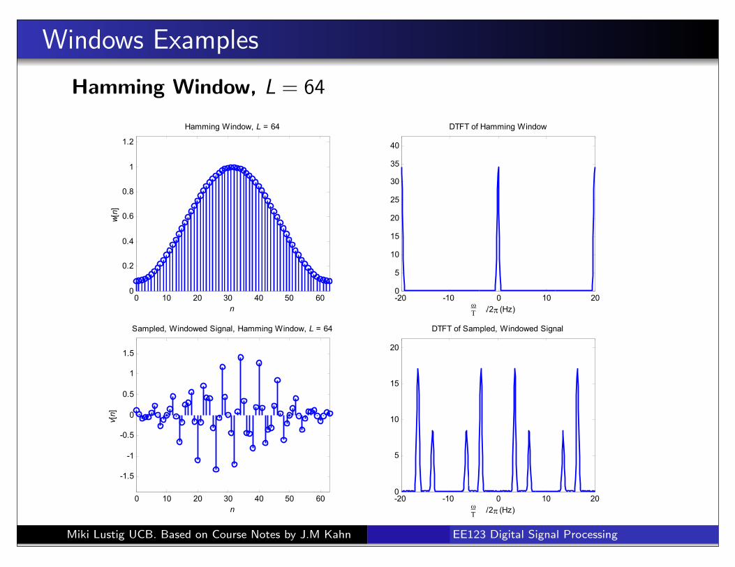
Windows Examples
Hamming Window, L = 64
0 10 20 30 40 50 600
0.2
0.4
0.6
0.8
1
1.2
n
w[n
]
Hamming Window, L = 64
-20 -10 0 10 200
5
10
15
20
25
30
35
40
/2 (Hz)
|W(ejT)|
DTFT of Hamming Window
0 10 20 30 40 50 60
-1.5
-1
-0.5
0
0.5
1
1.5
n
v[n]
Sampled, Windowed Signal, Hamming Window, L = 64
-20 -10 0 10 200
5
10
15
20
/2 (Hz)
|V(ejT)|
DTFT of Sampled, Windowed Signal
Miki Lustig UCB. Based on Course Notes by J.M Kahn Spring 2014, EE123 Digital Signal Processing
ωT
ωT

M. Lustig, EECS UC Berkeley
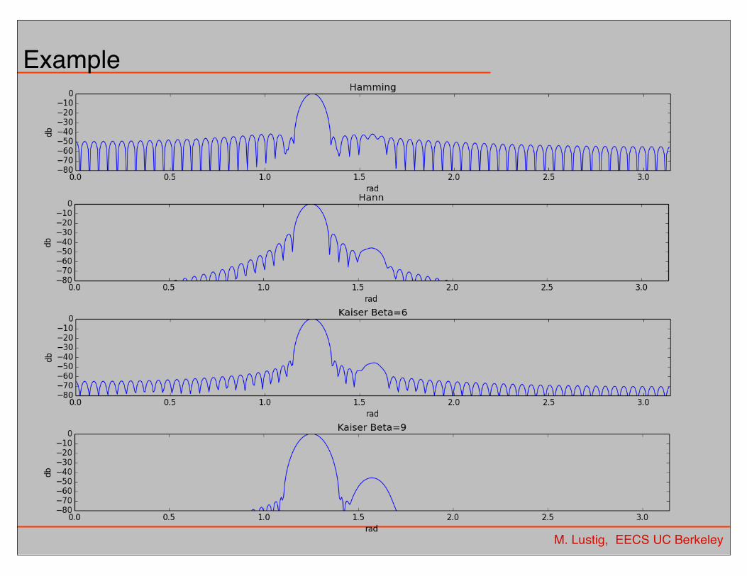
Optimal Window: Kaiser
• Minimum main-lobe width for a given side-lobe energy %
• Window is parametrized with L and β– β determines side-lobe level– L determines main-lobe width
Rsidelobes
|H(ej!)|2d!R ⇡�⇡ |H(ej!)|2d!
OS Eq 10.12
M. Lustig, EECS UC Berkeley
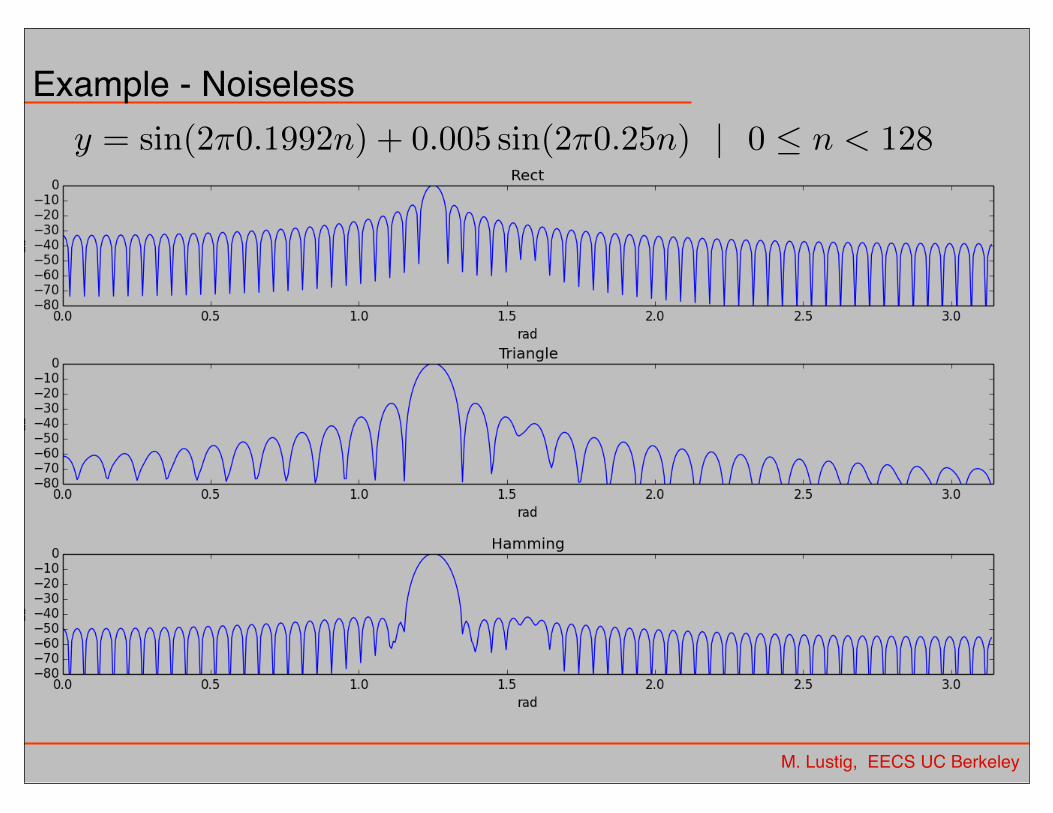
Example - Noiselessy = sin(2⇡0.1992n) + 0.005 sin(2⇡0.25n) | 0 n < 128
M. Lustig, EECS UC Berkeley
Example

Zero-Padding
In preparation for taking an N-point DFT, we may zero-padthe windowed block of signal samples to a block length N � L:
(v [n] 0 n L� 1
0 L n N � 1
This zero-padding has no e↵ect on the DTFT of v [n], sincethe DTFT is computed by summing over �1 < n < 1.
E↵ect of Zero Padding
We take the N-point DFT of the zero-padded v [n], to obtainthe block of N spectral samples:
V [k], 0 k N � 1
Miki Lustig UCB. Based on Course Notes by J.M Kahn Spring 2014, EE123 Digital Signal Processing
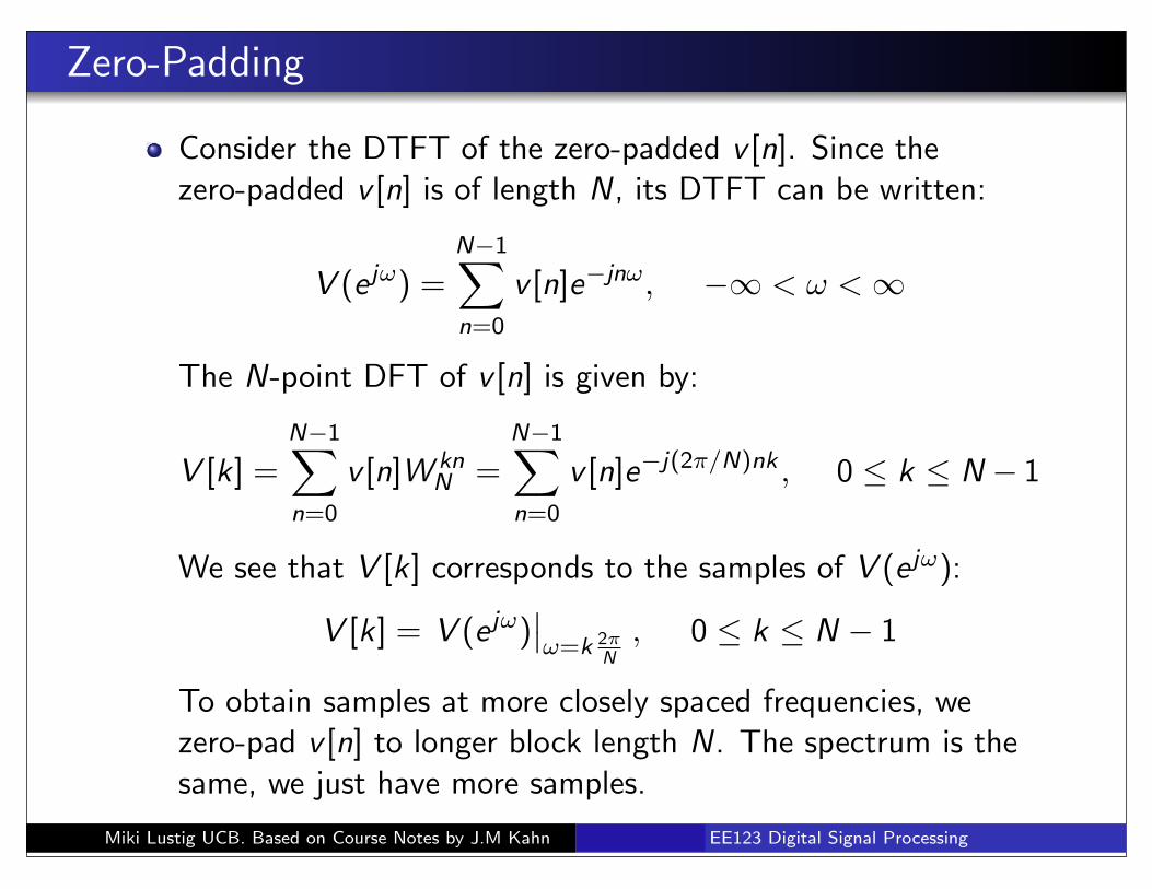
Zero-Padding
Consider the DTFT of the zero-padded v [n]. Since thezero-padded v [n] is of length N, its DTFT can be written:
V (e j!) =N�1X
n=0
v [n]e�jn!, �1 < ! < 1
The N-point DFT of v [n] is given by:
V [k] =N�1X
n=0
v [n]W kn
N
=N�1X
n=0
v [n]e�j(2⇡/N)nk , 0 k N � 1
We see that V [k] corresponds to the samples of V (e j!):
V [k] = V (e j!)��!=k
2⇡N
, 0 k N � 1
To obtain samples at more closely spaced frequencies, wezero-pad v [n] to longer block length N. The spectrum is thesame, we just have more samples.
Miki Lustig UCB. Based on Course Notes by J.M Kahn Spring 2014, EE123 Digital Signal Processing
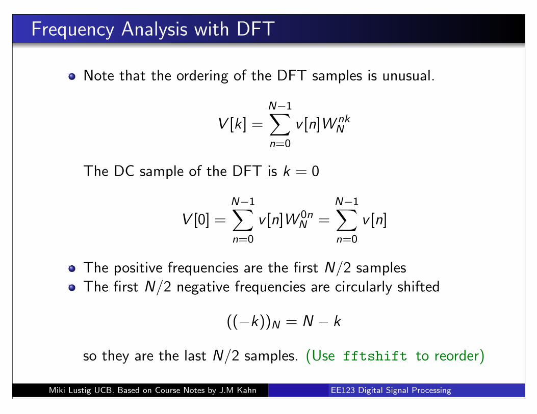
Frequency Analysis with DFT
Note that the ordering of the DFT samples is unusual.
V [k] =N�1X
n=0
v [n]W nk
N
The DC sample of the DFT is k = 0
V [0] =N�1X
n=0
v [n]W 0n
N
=N�1X
n=0
v [n]
The positive frequencies are the first N/2 samplesThe first N/2 negative frequencies are circularly shifted
((�k))N
= N � k
so they are the last N/2 samples. (Use fftshift to reorder)
Miki Lustig UCB. Based on Course Notes by J.M Kahn Spring 2014, EE123 Digital Signal Processing
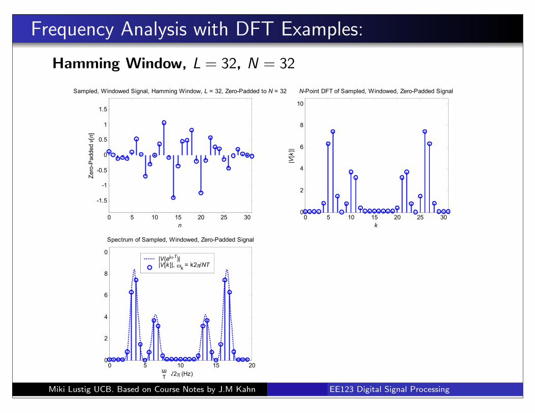
Frequency Analysis with DFT Examples:
Hamming Window, L = 32, N = 32
0 5 10 15 20 25 30
-1.5
-1
-0.5
0
0.5
1
1.5
n
Zero
-Padded v
[n]
Sampled, Windowed Signal, Hamming Window, L = 32, Zero-Padded to N = 32
0 5 10 15 20 25 300
2
4
6
8
10
k
|V[k
]|
N-Point DFT of Sampled, Windowed, Zero-Padded Signal
0 5 10 15 200
2
4
6
8
10
/2 (Hz)
|V[k
]|,
|V(ejT)|
Spectrum of Sampled, Windowed, Zero-Padded Signal
|V(ej T)||V[k ]|,
k = k2 /NT
Miki Lustig UCB. Based on Course Notes by J.M Kahn Spring 2014, EE123 Digital Signal Processing
ωT
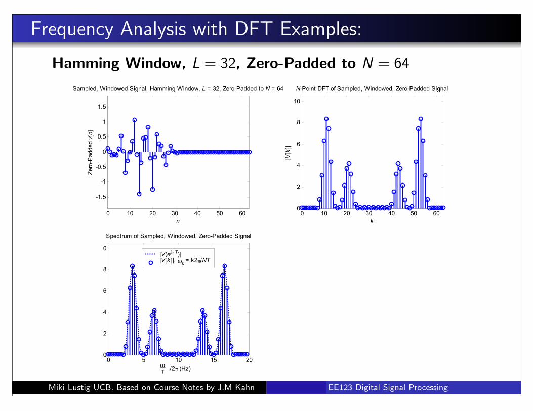
Frequency Analysis with DFT Examples:
Hamming Window, L = 32, Zero-Padded to N = 64
0 10 20 30 40 50 60
-1.5
-1
-0.5
0
0.5
1
1.5
n
Zero
-Padded v
[n]
Sampled, Windowed Signal, Hamming Window, L = 32, Zero-Padded to N = 64
0 10 20 30 40 50 600
2
4
6
8
10
k
|V[k
]|
N-Point DFT of Sampled, Windowed, Zero-Padded Signal
0 5 10 15 200
2
4
6
8
10
/2 (Hz)
|V[k
]|,
|V(ejT)|
Spectrum of Sampled, Windowed, Zero-Padded Signal
|V(ej T)||V[k ]|,
k = k2 /NT
Miki Lustig UCB. Based on Course Notes by J.M Kahn Spring 2014, EE123 Digital Signal Processing
ωT

000000000000000000000000000000000000000000000000000000000000000000000000000 0000000000000000000000000000000000000000000000000000000000000 00000000000 000000000000000000000000000000000000000000000000000000000000000000000000000 00000000000000000000000000000000000000000000000000
Rect window
iDFT20

000000000000000000000000000000000000000000000000000000000000000000000000000 0000000000000000000000000000000000000000000000000000000000000 00000000000 000000000000000000000000000000000000000000000000000000000000000000000000000 00000000000000000000000000000000000000000000000000
iDFT200
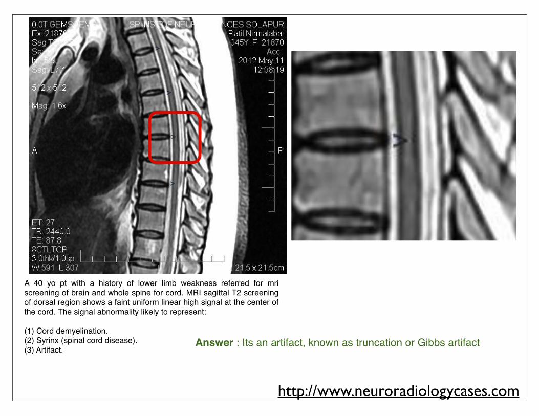
http://www.neuroradiologycases.com
A 40 yo pt with a history of lower limb weakness referred for mri screening of brain and whole spine for cord. MRI sagittal T2 screening of dorsal region shows a faint uniform linear high signal at the center of the cord. The signal abnormality likely to represent:
(1) Cord demyelination.(2) Syrinx (spinal cord disease).(3) Artifact.
Answer : Its an artifact, known as truncation or Gibbs artifact

Frequency Analysis with DFT
Length of window determines spectral resolution
Type of window determines side-lobe amplitude.(Some windows have better tradeo↵ betweenresolution-sidelobe)
Zero-padding approximates the DTFT better. Does notintroduce new information!
Miki Lustig UCB. Based on Course Notes by J.M Kahn Spring 2014, EE123 Digital Signal Processing
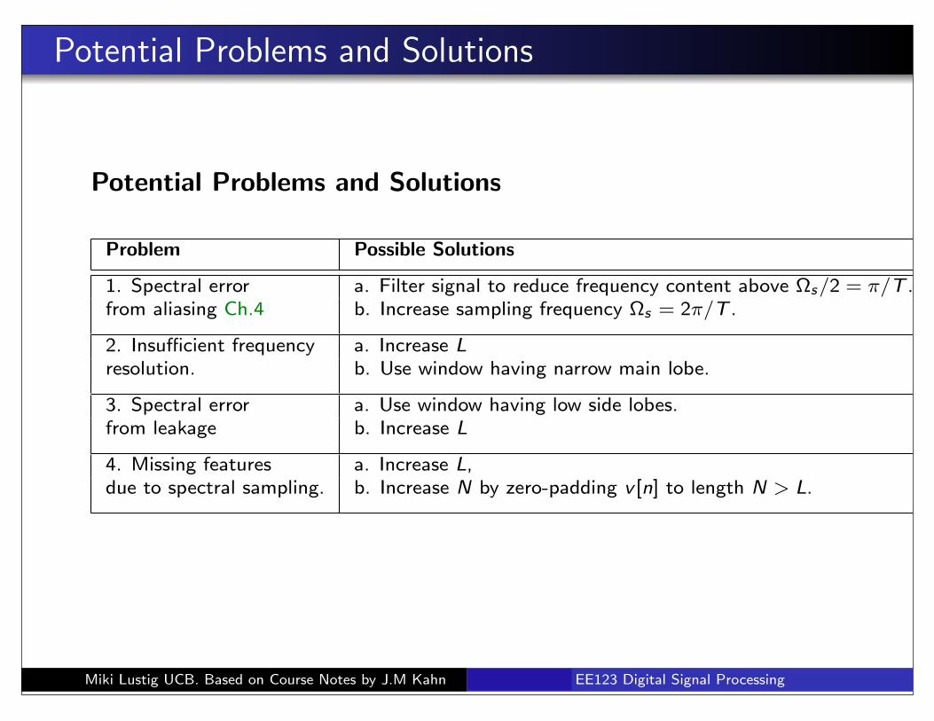
Potential Problems and Solutions
Potential Problems and Solutions
Problem Possible Solutions
1. Spectral error a. Filter signal to reduce frequency content above ⌦
s
/2 = ⇡/T .
from aliasing Ch.4 b. Increase sampling frequency ⌦
s
= 2⇡/T .
2. Insu�cient frequency a. Increase L
resolution. b. Use window having narrow main lobe.
3. Spectral error a. Use window having low side lobes.
from leakage b. Increase L
4. Missing features a. Increase L,
due to spectral sampling. b. Increase N by zero-padding v [n] to length N > L.
Miki Lustig UCB. Based on Course Notes by J.M Kahn Spring 2014, EE123 Digital Signal Processing