Dra

ft

EE 8235: Lectures 2 & 3 1

Lectures 2 & 3: Examples of distributed systems

• Simple PDEs

? Diffusion equation

? Linear transport equation

? Wave equation

? Evolution of population equation

• Not-so-simple PDEs

? Reaction-diffusion equation

? Swift-Hohenberg equation

? Navier-Stokes equations

Dra

ft

EE 8235: Lectures 2 & 3 2

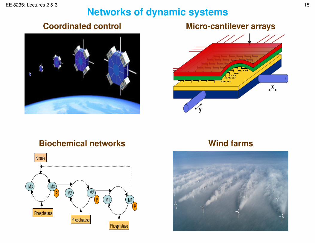
• Networks of dynamic systems

? Coordinated/cooperative control

? Leader selection in dynamic networks

? Micro-cantilever arrays

? Biochemical networks

? Wind farms

• Distributed control

? Feedback-based

? Sensor-free

Dra

ft

EE 8235: Lectures 2 & 3 3

Diffusion equation

∂φ(x, t)

∂t=

∂2φ(x, t)

∂x2+ u(x, t) ⇔ φt(x, t) = φxx(x, t) + u(x, t)

φ(x, t) – temperature at position x and time t

u(x, t) – heat addition along the bar

• Need to specify initial and boundary conditions

? One IC: φ(x, 0) = φ0(x)

? Two BCs:

Homogeneous Dirichlet: φ(±1, t) = 0

Homogeneous Neumann: φx(±1, t) = 0

Homogeneous Robin:aφ(−1, t) + b φx(−1, t) = 0

c φ(+1, t) + dφx(+1, t) = 0

Dra

ft

EE 8235: Lectures 2 & 3 4

• In higher spatial dimensions

φt(x, t) = ∆φ(x, t) + u(x, t)

x =[x1 · · · xn

]T – vector of spatial coordinates

∆ =∂2

∂x21+ · · · +

∂2

∂x2n– Laplacian

• Boundary actuation in 1D

φt(x, t) = φxx(x, t) + d(x, t)

φ(x, 0) = φ0(x)

φ(−1, t) = u(t), φ(+1, t) = 0

Dra

ft

EE 8235: Lectures 2 & 3 5

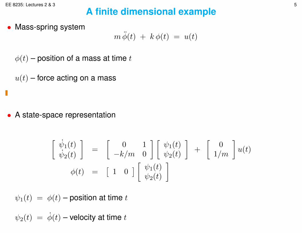
A finite dimensional example• Mass-spring system

mφ̈(t) + k φ(t) = u(t)

φ(t) – position of a mass at time t

u(t) – force acting on a mass

• A state-space representation

[ψ̇1(t)

ψ̇2(t)

]=

[0 1

−k/m 0

] [ψ1(t)ψ2(t)

]+

[0

1/m

]u(t)

φ(t) =[

1 0] [ ψ1(t)

ψ2(t)

]

ψ1(t) = φ(t) – position at time t

ψ2(t) = φ̇(t) – velocity at time t

Dra

ft

EE 8235: Lectures 2 & 3 6

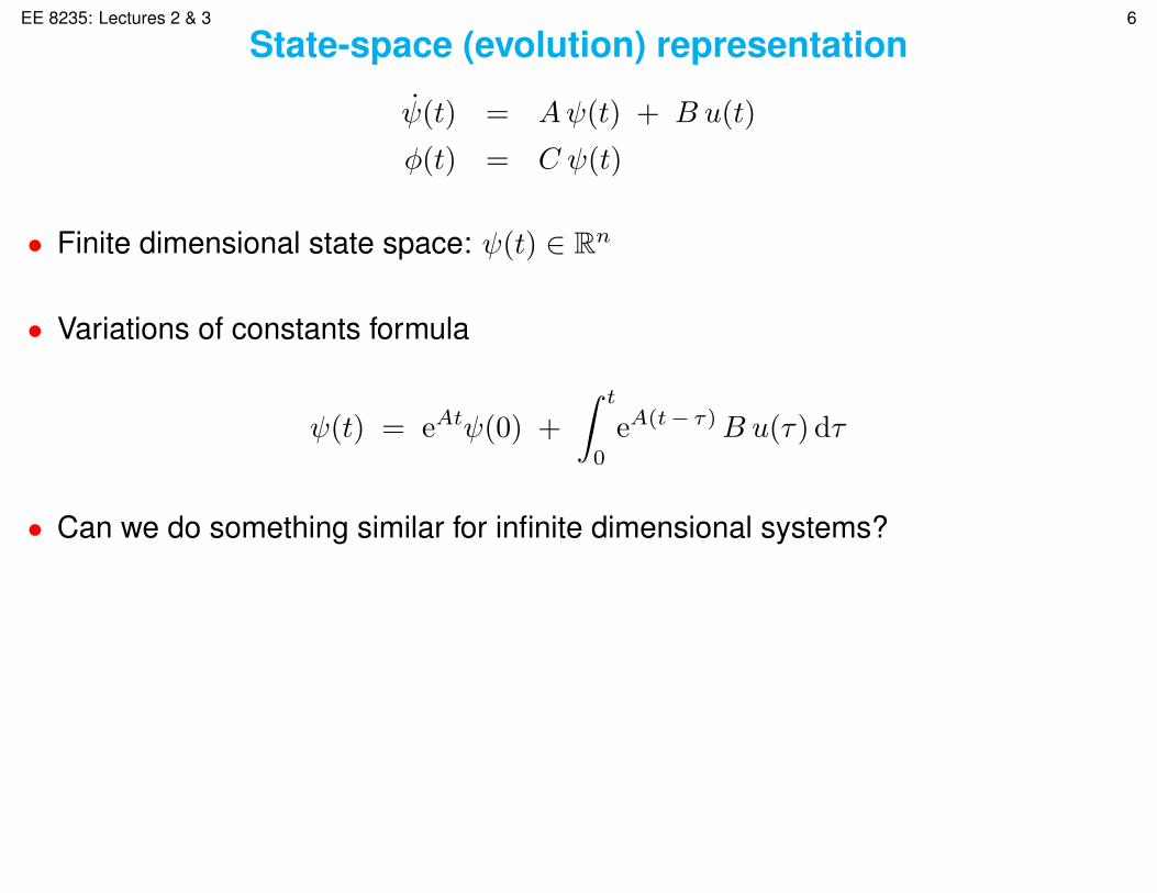
State-space (evolution) representation

ψ̇(t) = Aψ(t) + B u(t)

φ(t) = C ψ(t)

• Finite dimensional state space: ψ(t) ∈ Rn

• Variations of constants formula

ψ(t) = eAtψ(0) +

∫ t

0

eA(t− τ)B u(τ) dτ

• Can we do something similar for infinite dimensional systems?

Dra

ft

EE 8235: Lectures 2 & 3 7

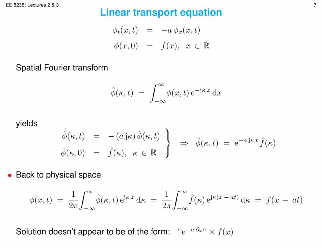
Linear transport equation

φt(x, t) = −aφx(x, t)

φ(x, 0) = f(x), x ∈ R

Spatial Fourier transform

φ̂(κ, t) =

∫ ∞−∞

φ(x, t) e−jκx dx

yields˙̂φ(κ, t) = − (a jκ) φ̂(κ, t)

φ̂(κ, 0) = f̂(κ), κ ∈ R

⇒ φ̂(κ, t) = e−a jκ t f̂(κ)

• Back to physical space

φ(x, t) =1

2π

∫ ∞−∞

φ̂(κ, t) ejκx dκ =1

2π

∫ ∞−∞

f̂(κ) ejκ(x− at) dκ = f(x − at)

Solution doesn’t appear to be of the form: ”e−a ∂x”× f(x)

Dra

ft

EE 8235: Lectures 2 & 3 8

Diffusion equation

φt(x, t) = φxx(x, t) + u(x, t)

φ(x, 0) = φ0(x)

φ(±1, t) = 0

Define ψ(t) = φ(·, t) and write an abstract evolution equation:

ψ̇(t) = Aψ(t) + u(t)

φ(t) = ψ(t)

• Infinite dimensional state-space: ψ(t) ∈ H

Dra

ft

EE 8235: Lectures 2 & 3 9

• A candidate for state-space

square-integrable functions: H = L2 [−1, 1] =

{f,

∫ 1

−1f∗(x) f(x) dx < ∞

}

• A =d2

dx2+ boundary conditions (contained in the domain of A)

D(A) =

{f ∈ L2 [−1, 1],

d2f

dx2∈ L2 [−1, 1], f(±1) = 0

}

Dra

ft

EE 8235: Lectures 2 & 3 10

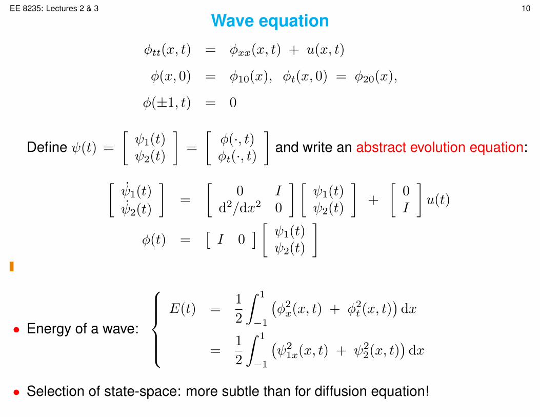
Wave equation

φtt(x, t) = φxx(x, t) + u(x, t)

φ(x, 0) = φ10(x), φt(x, 0) = φ20(x),

φ(±1, t) = 0

Define ψ(t) =

[ψ1(t)ψ2(t)

]=

[φ(·, t)φt(·, t)

]and write an abstract evolution equation:

[ψ̇1(t)

ψ̇2(t)

]=

[0 I

d2/dx2 0

] [ψ1(t)ψ2(t)

]+

[0I

]u(t)

φ(t) =[I 0

] [ ψ1(t)ψ2(t)

]

• Energy of a wave:

E(t) =

1

2

∫ 1

−1

(φ2x(x, t) + φ2t (x, t)

)dx

=1

2

∫ 1

−1

(ψ21x(x, t) + ψ2

2(x, t))

dx

• Selection of state-space: more subtle than for diffusion equation!

Dra

ft

EE 8235: Lectures 2 & 3 11

Evolution of population equation

φt(x, t) = −φx(x, t) − µ(x, t)φ(x, t)

φ(x, 0) = φ0(x) x ≥ 0,

φ(0, t) = u(t), t ≥ 0

φ(x, t) – number of people of age x at time t

µ(x, t) – mortality function

φ0(x) – initial age distribution

u(t) – number of people born at time t

• Control problem: design u to achieve desired age profile φd(x) at time T

Dra

ft

EE 8235: Lectures 2 & 3 12

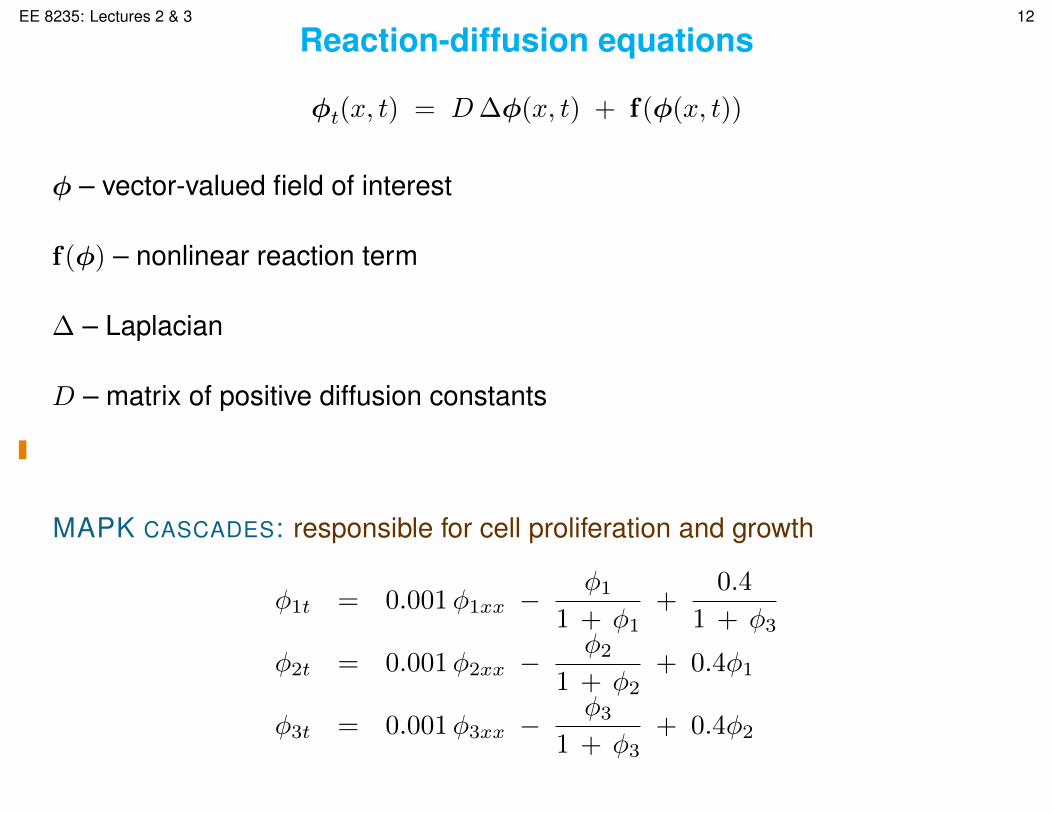
Reaction-diffusion equations

φt(x, t) = D∆φ(x, t) + f(φ(x, t))

φ – vector-valued field of interest

f(φ) – nonlinear reaction term

∆ – Laplacian

D – matrix of positive diffusion constants

MAPK CASCADES: responsible for cell proliferation and growth

φ1t = 0.001φ1xx −φ1

1 + φ1+

0.4

1 + φ3

φ2t = 0.001φ2xx −φ2

1 + φ2+ 0.4φ1

φ3t = 0.001φ3xx −φ3

1 + φ3+ 0.4φ2

Dra

ft

EE 8235: Lectures 2 & 3 13

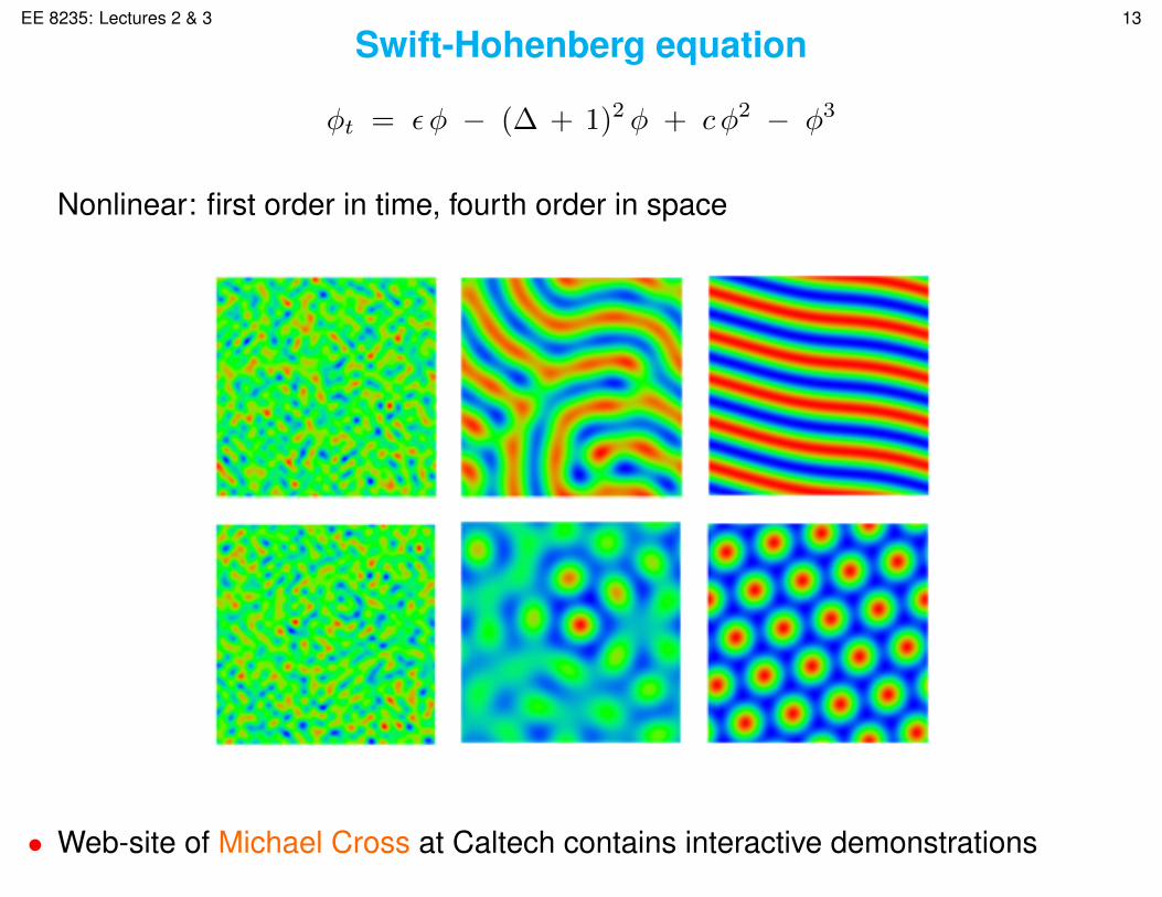
Swift-Hohenberg equation

φt = ε φ − (∆ + 1)2 φ + c φ2 − φ3

Nonlinear: first order in time, fourth order in space

• Web-site of Michael Cross at Caltech contains interactive demonstrations

Dra

ft

EE 8235: Lectures 2 & 3 14

Navier-Stokes equations

conservation of momentum: vt = − (v · ∇)v − ∇p + (1/Re) ∆v + d

conservation of mass: 0 = ∇ · v

Describe the fluid motion

Nonlinear system of equations for:

pressure: p(x1, x2, x3, t)

velocity: v =[v1 v2 v3

]T“del” operator: ∇ =

∂

∂x1e1 +

∂

∂x2e2 +

∂

∂x3e3

Reynolds number: Re =inertial forcesviscous forces

Dra

ft

EE 8235: Lectures 2 & 3 15

Networks of dynamic systemsCoordinated control Micro-cantilever arrays

Biochemical networks Wind farms

Cyclic Biochemical Networks with Inhibitory Feedback

Gene Regulation: Jacob & Monod (‘61), Goodwin (‘65), Elowitz & Leibler (2000)

: DNA : mRNA : enzyme : endproduct

Cellular Signaling: Kholodenko (2000), Shvartsman et al. (2001), and others

Kinase

M3P

Phosphatase

M3M2

Phosphatase

M2M1

Phosphatase

M1PP

Metabolic Pathways: Morales and McKay (‘67), Stephanopoulos et al. (‘98)

Dra

ft

EE 8235: Lectures 2 & 3 16

Feedback flow control

• CHALLENGES

? control-oriented modeling of turbulent flows

? design of estimators for turbulent flows

? design of spatially localized distributed controllers

? design of controllers of low dynamical order

Dra

ft

EE 8235: Lectures 2 & 3 17

Flow control in nature . . .

. . . and in swimming competitions

Dra

ft

EE 8235: Lectures 2 & 3 18

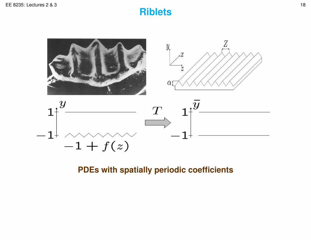
Riblets

PDEs with spatially periodic coefficients

Dra

ft

EE 8235: Lectures 2 & 3 19

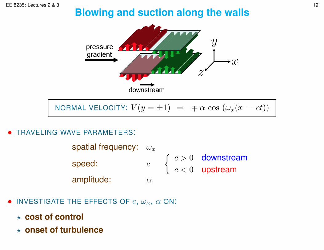
Blowing and suction along the walls

NORMAL VELOCITY: V (y = ±1) = ∓ α cos (ωx(x − ct))

• TRAVELING WAVE PARAMETERS:

spatial frequency: ωx

speed: c

{c > 0 downstreamc < 0 upstream

amplitude: α

• INVESTIGATE THE EFFECTS OF c, ωx, α ON:

? cost of control? onset of turbulence