EE 583 PATTERN RECOGNITION Supervised Learning
47
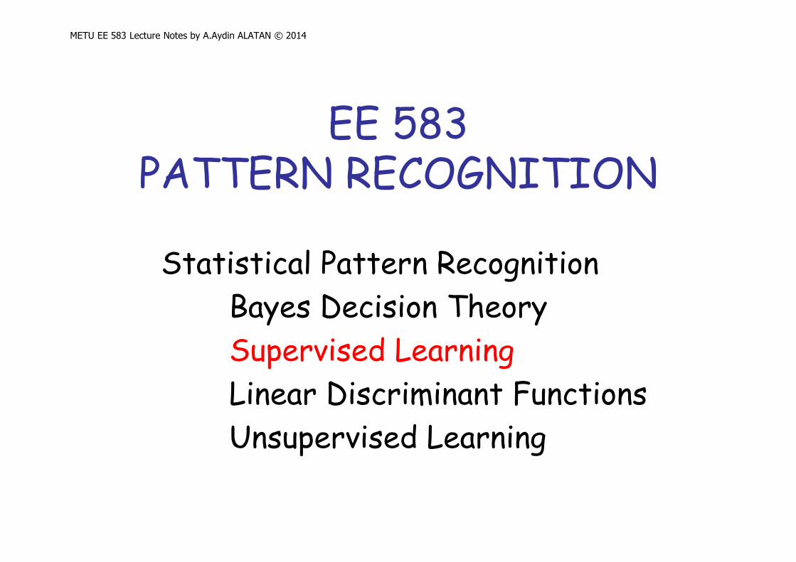
METU EE 583 Lecture Notes by A.Aydin ALATAN © 2014 EE 583 PATTERN RECOGNITION Statistical Pattern Recognition Bayes Decision Theory Supervised Learning Linear Discriminant Functions Unsupervised Learning
Transcript of EE 583 PATTERN RECOGNITION Supervised Learning
METU EE 583 Lecture Notes by A.Aydin ALATAN © 2014
EE 583 PATTERN RECOGNITION
Statistical Pattern Recognition
Bayes Decision Theory
Supervised Learning
Linear Discriminant Functions
Unsupervised Learning

METU EE 583 Lecture Notes by A.Aydin ALATAN © 2014
Supervised Learning
� Supervised Learning == Training� Parametric approaches
� Maximum likelihood estimation� Bayesian parameter estimation
� Non-parametric approaches� Direct pdf (multi-D histogram) estimation� Parzen window pdf estimation� kn-nearest neighbor pdf estimation� Nearest-neighbor rule

METU EE 583 Lecture Notes by A.Aydin ALATAN © 2014
Parametric Approaches� “Curse of dimensionality” : We need lots of
training data to determine the completely unknown statistics for multi-D problems� A rule of thumb : “use at least 10 times as many
training samples per class as the number of features (i.e. D)”
� Hence, with some a priori information, it is possible to estimate the parameters of the known distribution by using less number of samples

METU EE 583 Lecture Notes by A.Aydin ALATAN © 2014
Maximum Likelihood Estimation (1/4)Assume c sets of samples, drawn according to
)|( jxp ω which has a known parametric form.
e.g. pdf is known to be Gaussian; mean & variance values are unknown
jΘr
Let be unknown deterministic parameter set of pdf for class-j
Aim : Use the information provided by the observedsamples to estimate the unknown parameter
),|()|( jjj xpxp Θ=r
ωω : shows the dependence
Note that all sets of samples have independent pdf’s,
� there are c separate problems

METU EE 583 Lecture Notes by A.Aydin ALATAN © 2014
Maximum Likelihood Estimation (2/4)
∏=
Θ=Θn
kkxpXp
1
)|()|(rr
For an arbitrary class, let an observed sample set, X, contain n samples, X={ x1,…,xn} .
Find value of the parameter that maximizes )|( Θr
Xp
� In order to find the parameter that maximizes its value, differentiate the conditional probability and equate to zero
Assume the samples are independently drawn from their density, )|( Θ
r
xp
The likelihood of the observed sample set, X :
METU EE 583 Lecture Notes by A.Aydin ALATAN © 2014
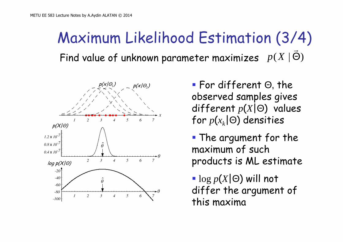
Maximum Likelihood Estimation (3/4)Find value of unknown parameter maximizes )|( Θ
r
Xp
� For different Θ, the observed samples gives different p(X|Θ) values for p(xk|Θ) densities
� The argument for the maximum of such products is ML estimate
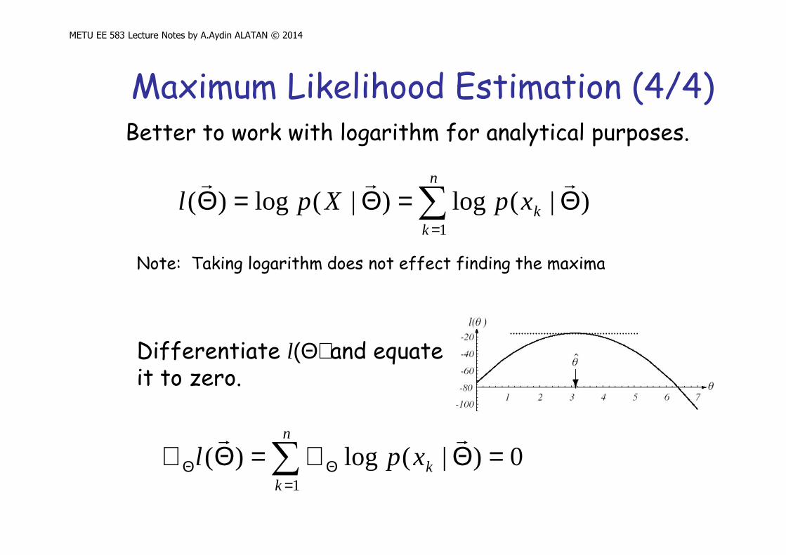
� log p(X|Θ) will not differ the argument of this maxima
p(X|Θ)
log p(X|Θ)
p(x|Θ1) p(x|Θ2)
METU EE 583 Lecture Notes by A.Aydin ALATAN © 2014
Maximum Likelihood Estimation (4/4)
∑=
Θ=Θ=Θn
kkxpXpl
1
)|(log)|(log)(rrr
Better to work with logarithm for analytical purposes.
0)|(log)(1
=Θ∇=Θ∇ ∑=
ΘΘ
n
kkxpl
rr
Differentiate l(Θ) and equate it to zero.
Note: Taking logarithm does not effect finding the maxima

METU EE 583 Lecture Notes by A.Aydin ALATAN © 2014
ML Estimate of Univariate Normal :
21
22 )(
2
1})2log{(
2
1)|(log θ
θθπ −−−=Θ kk xxp
Assume mean θ1 & variance θ22 are unknown for a Gaussian pdf:
−+−
−=Θ∇Θ
22
21
2
12
2
)(
2
1
)(1
)|(log
θθ
θ
θθ
k
k
k x
x
xpDifferentiate wrt θ1 and θ2 :
Maximum likelihood estimates of the parameters :
∑∑∑
∑∑
===
==
−=⇒=−+−
=⇒=−
n
kk
n
k
kn
k
n
kk
n
kk
xn
x
xn
x
1
212
12
2
21
1 2
11
11
2
)ˆ(1ˆ0
)(1
1ˆ0)(1
θθθ
θθ
θθθ
ML estimates of mean and variance

METU EE 583 Lecture Notes by A.Aydin ALATAN © 2014
ML Estimate of Multivariate Normal :
)()(2
1|}|)2log{(
2
1)|(log 1 µµπµ rrrrrr −Σ−−Σ−= −
kt
kd
k xxxp
Assume only mean vector is unknown :
)()|(log 1 µµµrrrr −Σ=∇ −
kk xxp
Differentiate
Maximum likelihood estimate of the unknown mean vector :
∑∑==
− =⇒=−Σn
kk
n
kk x
nx
11
1 1ˆ0)(rrrr µµ
MLE of mean is the arithmetic average of vector samples
METU EE 583 Lecture Notes by A.Aydin ALATAN © 2014
Bayesian Parameter Estimation (1/3)
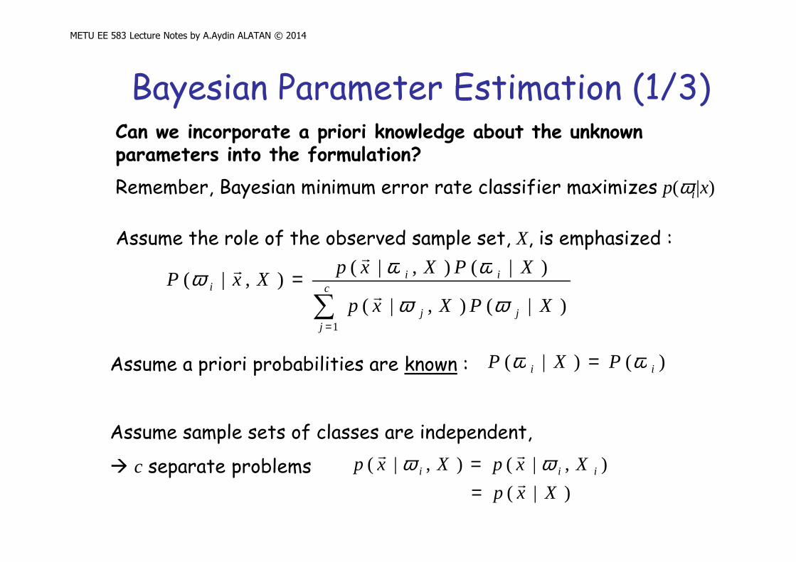
Assume the role of the observed sample set, X, is emphasized :
∑=
= c
jjj
iii
XPXxp
XPXxpXxP
1
)|(),|(
)|(),|(),|(
ωω
ωωωr
r
r
Assume sample sets of classes are independent,
� c separate problems
Assume a priori probabilities are known : )()|( ii PXP ωω =
)|(
),|(),|(
Xxp
XxpXxp iiir
rr
== ωω
Can we incorporate a priori knowledge about the unknown parameters into the formulation?
Remember, Bayesian minimum error rate classifier maximizes p(ωi|x)

METU EE 583 Lecture Notes by A.Aydin ALATAN © 2014
Bayesian Parameter Estimation (2/3)
Samples are drawn independently according to whose parametric form is known
)|( Θxpr
Bayesian approach assumes that the unknown parameter is a random variable with a known density )(Θp
∑=
=c
jjj PXxp
PXxpXxP
1
)(),|(
)()|(),|(
ωω
ωωr
r
r
Main aim is to compute )|( Xxpr
ΘΘΘ=ΘΘ= ∫ ∫ dXpxpdXxpXxpknownisform
4342143421
rrr
?
)|()|()|,()|(
METU EE 583 Lecture Notes by A.Aydin ALATAN © 2014
Bayesian Parameter Estimation (3/3)
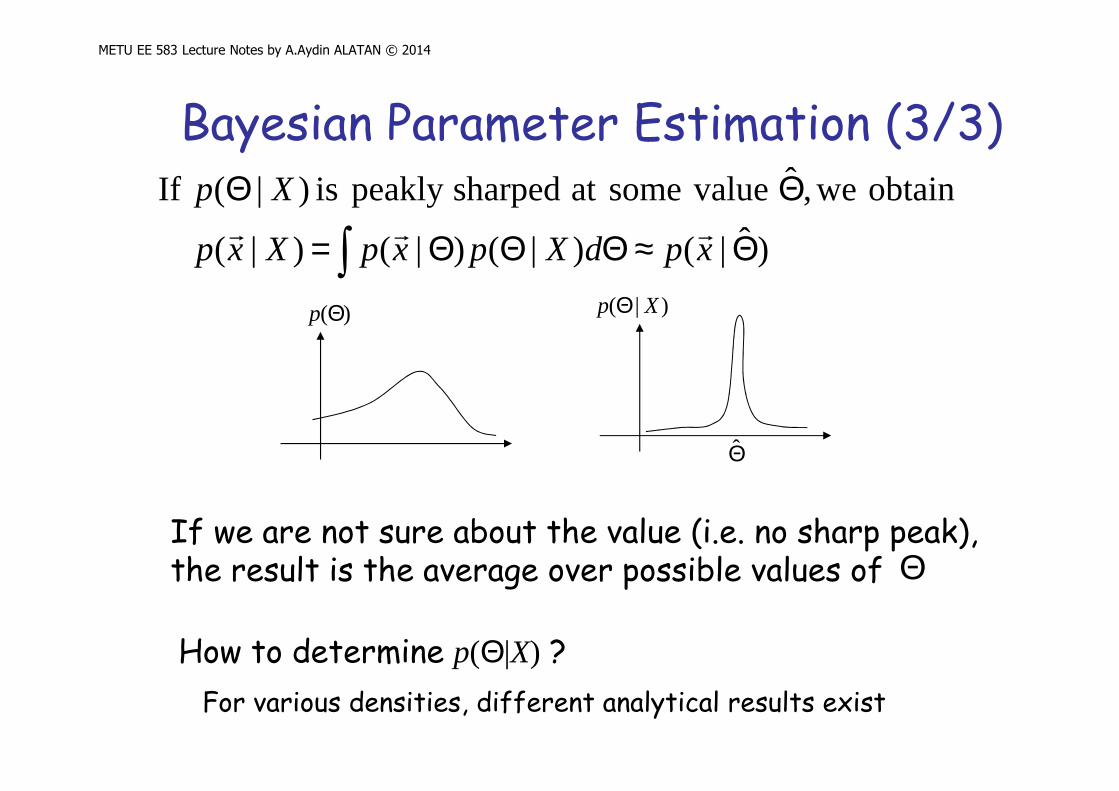
)ˆ|()|()|( )|(
obtain we,ˆ valuesome at sharped peakly is )|( If
Θ≈ΘΘΘ=
ΘΘ
∫ xpdXpxpXxp
Xprrr
If we are not sure about the value (i.e. no sharp peak), the result is the average over possible values of Θ
)(Θp )|( Xp Θ
Θ̂
How to determine p(Θ|X) ?
For various densities, different analytical results exist

METU EE 583 Lecture Notes by A.Aydin ALATAN © 2014
Bayesian Parameter EstimationUnivariate Normal Distribution (1/3)
A univariate normal distribution with unknown µ),(~)|( 2σµµ Nxp
A priori information about µ is expressed by density),(~)( 2
00 σµµ Np
Observing the sample set, D, p(µ|D) becomes
∏∫ =
==n
kk pxp
dpDp
pDpDp
1
)()|()()|(
)()|()|( µµα
µµµµµµ
=
−−
=
−−
∏2
0
02 )(2
1
01
)(2
1
2
1
2
1)|( σ
µµσ
µ
σπσπαµ eeDp
n
k
xk

METU EE 583 Lecture Notes by A.Aydin ALATAN © 2014
Bayesian Parameter EstimationUnivariate Normal Distribution (2/3)
+−+−
−+−− ∑′′=
∑′= ==
µσµ
σµ
σσσµµ
σµ
ααµ)
1(2)
1(
2
1)()(
2
1
120
02
220
22
0
0
1
2
)|(
n
kk
n
k
k xnx
eeDp
{22
0
20
22
0220
2
1
220
202 ;,),(~)|(
σσσσ
σµσσ
σσσ
σµσµµ+
=+
+
∑+
=⇒nn
mn
nNDp n
xn
nnnn
k
Increasing number of samples� p(µ|D) sharper peak
As n�∞, p(µ|D) � δ(µ) � Bayesian Learning

METU EE 583 Lecture Notes by A.Aydin ALATAN © 2014
Bayesian Parameter EstimationUnivariate Normal Distribution (3/3)
∫= µµµ dDpxpDxp )|()|()|(
After determining p(µ|D), p(x|D) is obtained by
µσπσπ
σµµ
σµ
deeDxp n
n
n
x
=⇒
−−−−
∫22 )(
2
1)(
2
1
2
1
2
1)|(
),(~)|(
),(2
1)|(
22
)(
2
122
2
nn
n
x
n
NDxp
feDxp n
n
σσµ
σσσσπ
σσµ
+⇒
=⇒ +−−
Compared to the initial knowledge, p(x|µ), about µ, p(x|D) has additional uncertainty due to lack of exact knowledge of µ.

METU EE 583 Lecture Notes by A.Aydin ALATAN © 2014
General Bayesian Learning
• The form of the density, p(x|Θ), is assumed to be known, but the value of parameter, Θ, is unknown
• Our initial knowledge about the parameter, Θ, is assumed to be contained in a known a priori density, p(Θ).
• The rest of our knowledge about the parameter, Θ, is contained in n samples, drawn according to the unknown probability p(x|Θ)
In summary :

METU EE 583 Lecture Notes by A.Aydin ALATAN © 2014
Comparison : ML vs. Bayesian
� ML avoids many assumptions and analytically easier to solve, although some estimates can be biased
� Bayesian parameter estimation permits including a priori information about the unknown, but the analytical derivations are cumbersome.
� For ordinary cases, both approaches give similar results with sufficient sample data

METU EE 583 Lecture Notes by A.Aydin ALATAN © 2014
Non-Parametric Approaches
� Parametric approaches require� Knowing the form of the density
� Finding the parameter of the density
� In many cases,� The form is not known
� The form does not let you to find a unique solution (multi-modal densities)

METU EE 583 Lecture Notes by A.Aydin ALATAN © 2014
Non-Parametric Approaches
� The solution is to use non-parametric approaches which do not assume a form
� There are 2 main directions :� Estimating densities non-parametrically
� Direct estimation of density� Parzen window� k-NN estimation
� Nearest Neighbor Rules

METU EE 583 Lecture Notes by A.Aydin ALATAN © 2014
Non-Parametric ApproachesDensity Estimation (1/3)
Probability P of a vector x falling into region R :
∫ℜ
′′= xdxpPrr
)(
N samples of x independently drawn according to p(x)
Probability of k independent samples fall into R (Binomial):
)1()var(,][)1( PnPknPkEandPPk
nP knk
k −==−
= −
Since Binomial distribution peaks very sharply around the expected value, the number of observed samples (kobs) in Rshould be approximately equal nPkEkobs =≈ ][
Note that probability P can be estimated via , but we need density, p(x)
nkP obs /≈
METU EE 583 Lecture Notes by A.Aydin ALATAN © 2014
Non-Parametric ApproachesDensity Estimation (2/3)
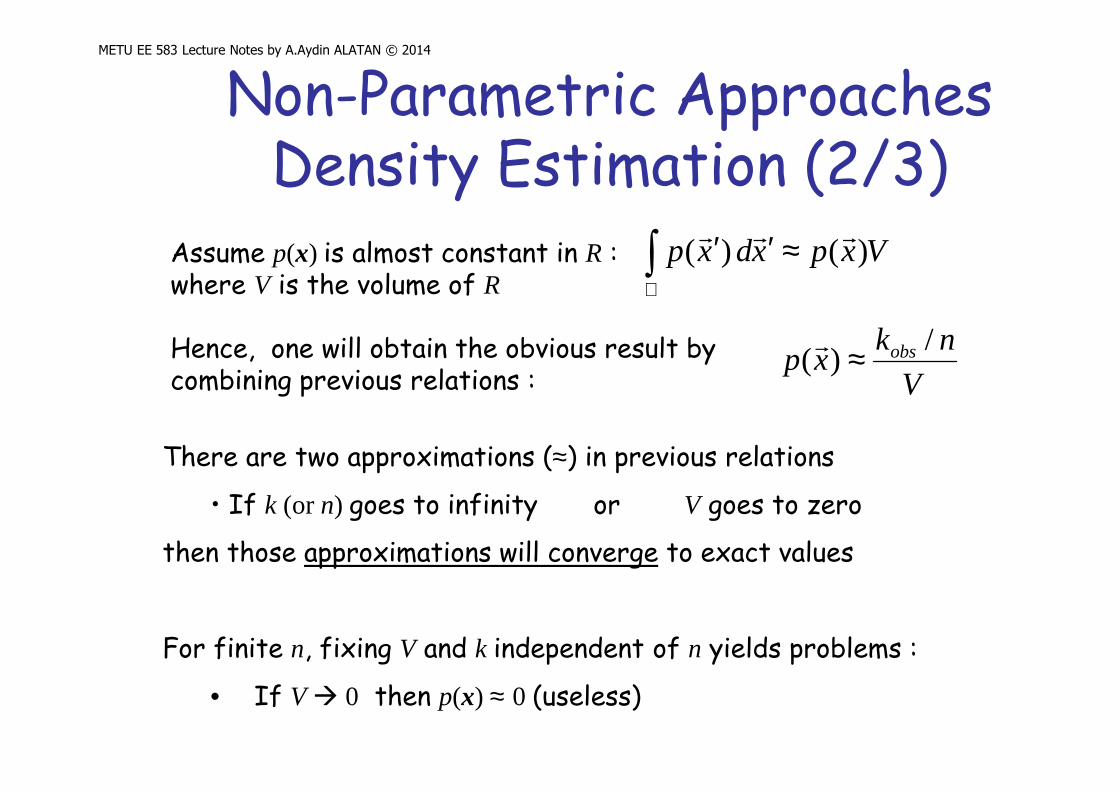
Assume p(x) is almost constant in R : where V is the volume of R
Vxpxdxp )()(rrr ≈′′∫
ℜ
Hence, one will obtain the obvious result by combining previous relations : V
nkxp obs /)( ≈r
There are two approximations (≈) in previous relations
• If k (or n) goes to infinity or V goes to zero
then those approximations will converge to exact values
For finite n, fixing V and k independent of n yields problems :
• If V � 0 then p(x) ≈ 0 (useless)

METU EE 583 Lecture Notes by A.Aydin ALATAN © 2014
Examples that achieve these conditions :
• Parzen : Initial Vo volume is shrinking
• k-NN : Rn is grown until it contains kn samples
Non-Parametric ApproachesDensity Estimation (3/3)
)()(lim xpxdxpnn
rrr =′′∫ℜ
∞→3 conditions under which
n
nn V
nkxp
/)( ≡r
0lim)3(lim)2(0lim)1( =∞==∞→∞→∞→ n
kkV n
nn
nn
n
n
VVn
0=
nkn =
Form a sequence of regions, Rn ,centered at x for n samples
METU EE 583 Lecture Notes by A.Aydin ALATAN © 2014
Non-Parametric ApproachesParzen Windows (1/2)
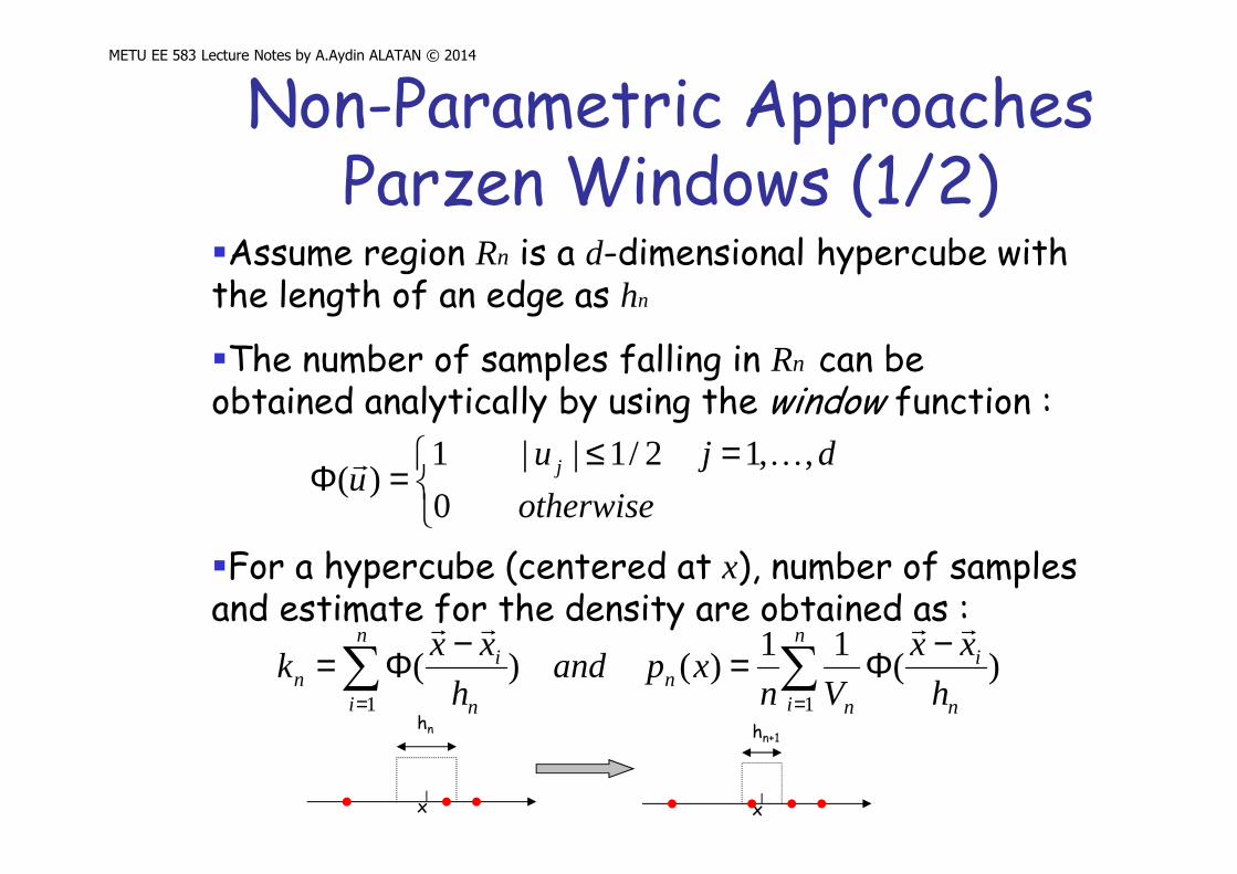
�Assume region Rn is a d-dimensional hypercube with the length of an edge as hn
=≤
=Φotherwise
djuu j
0
,,12/1||1)(
Kr
�The number of samples falling in Rn can be obtained analytically by using the window function :
∑∑==
−Φ=−Φ=n
i n
i
n
n
in
n
in h
xx
Vnxpand
h
xxk
11
)(11
)()(rrrr
�For a hypercube (centered at x), number of samples and estimate for the density are obtained as :
x
hn
x
hn+1
METU EE 583 Lecture Notes by A.Aydin ALATAN © 2014
Non-Parametric ApproachesParzen Windows (2/2)
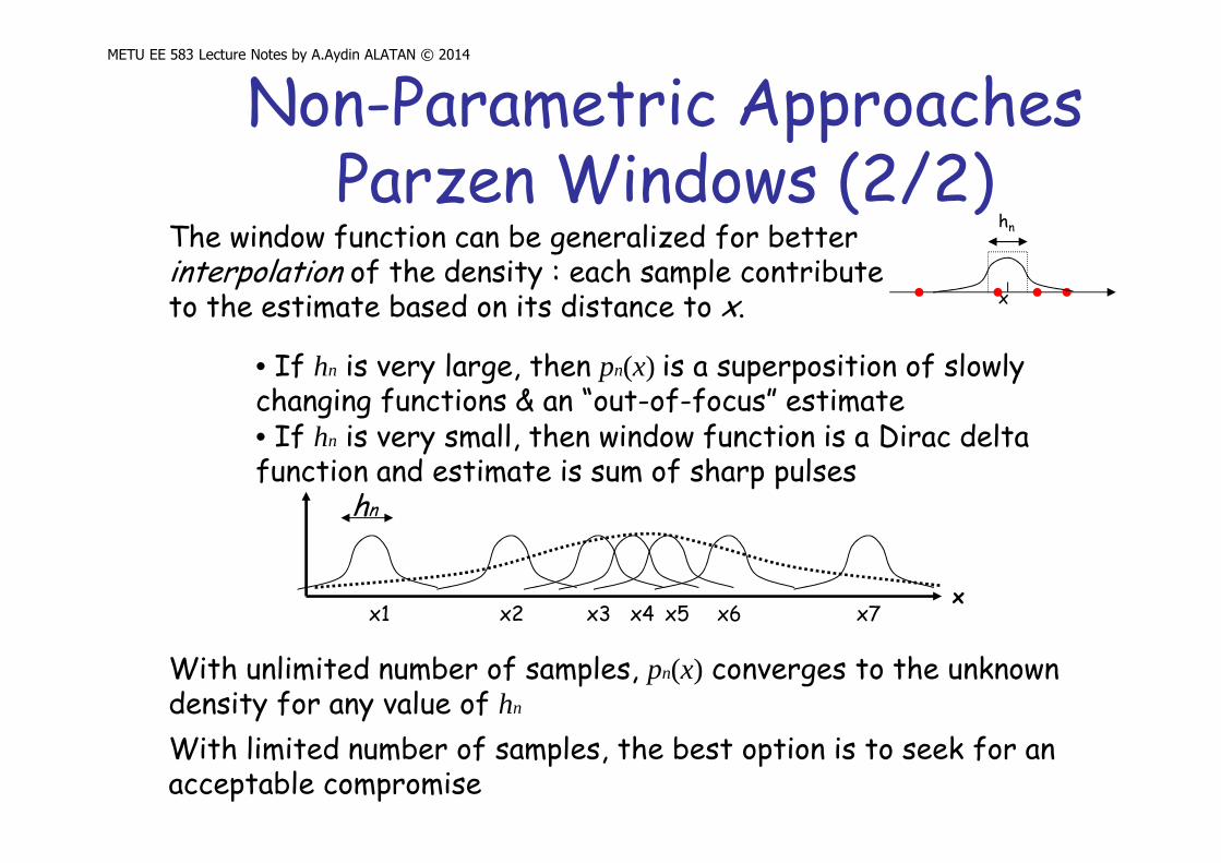
The window function can be generalized for better interpolation of the density : each sample contribute to the estimate based on its distance to x.
• If hn is very large, then pn(x) is a superposition of slowly changing functions & an “out-of-focus” estimate• If hn is very small, then window function is a Dirac delta function and estimate is sum of sharp pulses
With unlimited number of samples, pn(x) converges to the unknown density for any value of hn
With limited number of samples, the best option is to seek for an acceptable compromise
x1 x2 x3 x4 x5 x6 x7x
hn
x
hn
METU EE 583 Lecture Notes by A.Aydin ALATAN © 2014
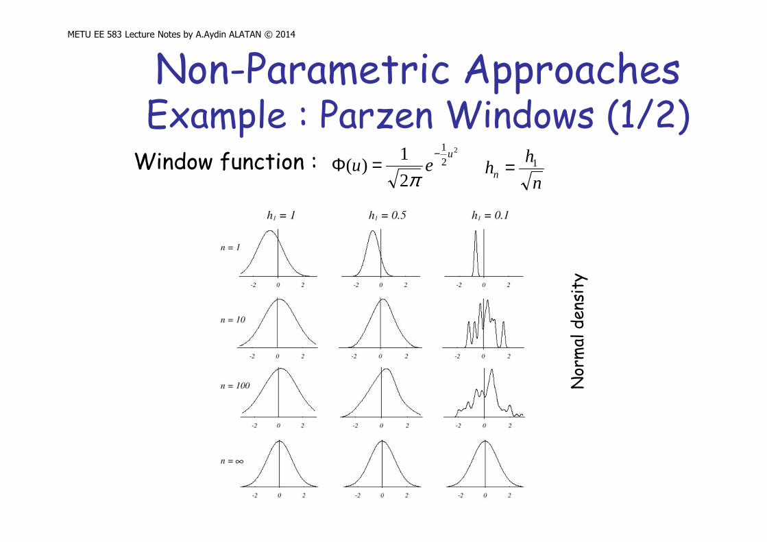
Non-Parametric ApproachesExample : Parzen Windows (1/2)
Window function : 2
2
1
2
1)(
ueu
−=Φ
π n
hhn
1=
Nor
mal
den
sity
METU EE 583 Lecture Notes by A.Aydin ALATAN © 2014
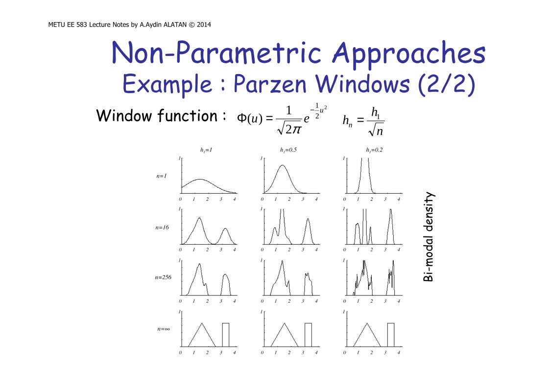
Non-Parametric ApproachesExample : Parzen Windows (2/2)
Window function : 2
2
1
2
1)(
ueu
−=Φ
π n
hhn
1=
Bi-
mod
al d
ensi
ty
METU EE 583 Lecture Notes by A.Aydin ALATAN © 2014
Non-Parametric Approacheskn-Nearest Neighbor
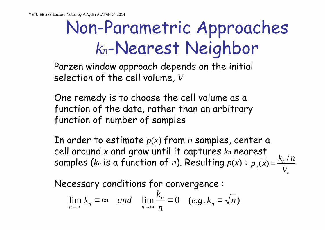
Parzen window approach depends on the initial selection of the cell volume, V
One remedy is to choose the cell volume as a function of the data, rather than an arbitrary function of number of samples
In order to estimate p(x) from n samples, center a cell around x and grow until it captures kn nearestsamples (kn is a function of n). Resulting p(x) :
n
nn V
nkxp
/)( =
)..(0limlim nkgen
kandk n
n
nn
n==∞=
∞→∞→
Necessary conditions for convergence :

METU EE 583 Lecture Notes by A.Aydin ALATAN © 2014
Non-Parametric ApproachesExample : kn-Nearest Neighbor

METU EE 583 Lecture Notes by A.Aydin ALATAN © 2014
Non-Parametric ApproachesParzen vs kn-Nearest Neighbor
Both methods do converge, but it is very difficult to make meaningful statements about their finite-sample behaviour

METU EE 583 Lecture Notes by A.Aydin ALATAN © 2014
Non-Parametric ApproachesClassification Rule
All 3 methods (direct, Parzen, kn-NN) can be used to obtain a posteriori probabilities for n-sample data
n
iin V
nkxp
/),( =ω k
k
xp
xpxP i
c
jjn
inin ==
∑=1
),(
),()|(
ω
ωω
At each cell, total k samples; ki samples for each class
Cell size selection can be achieved by using either Parzen window or kn-NN approach
Using arbitrarily large number of samples, unknown probabilities can be obtained with optimum performance

METU EE 583 Lecture Notes by A.Aydin ALATAN © 2014
Non-Parametric ApproachesNearest Neighbor Rule (1/3)
All 3 methods (direct, Parzen, kn-NN) can be used to obtain a posteriori probabilities by using n-sample data so that this density is utilized for Bayes Decision Rule
A radical approach is to use the nearest neighbor out of the sample data to classify the unknown test data (Nearest Neighbor Rule [NN-R])
While Bayes Rule (minimum-error rate) is optimal while choosing between different classes, NN-R is suboptimal

METU EE 583 Lecture Notes by A.Aydin ALATAN © 2014
Assume that there are unlimited number of labeled “prototypes” for each class
If the test point x is nearest to one of these prototypes, x’ � p(wi|x) ≈ p(wi|x’) for all i
Obviously, x’ labeled with m gives p(wm |x’) > p(wj|x’) for all j ≠ m
� one should expect p(wm |x) > p(wj|x) for all j ≠ m
For unlimited samples, the error rate for NN-R is less than twice the error rate of Bayes decision rule
Non-Parametric ApproachesNearest Neighbor Rule (2/3)
METU EE 583 Lecture Notes by A.Aydin ALATAN © 2014
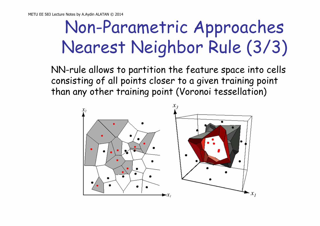
Non-Parametric ApproachesNearest Neighbor Rule (3/3)
NN-rule allows to partition the feature space into cells consisting of all points closer to a given training point than any other training point (Voronoi tessellation)
METU EE 583 Lecture Notes by A.Aydin ALATAN © 2014
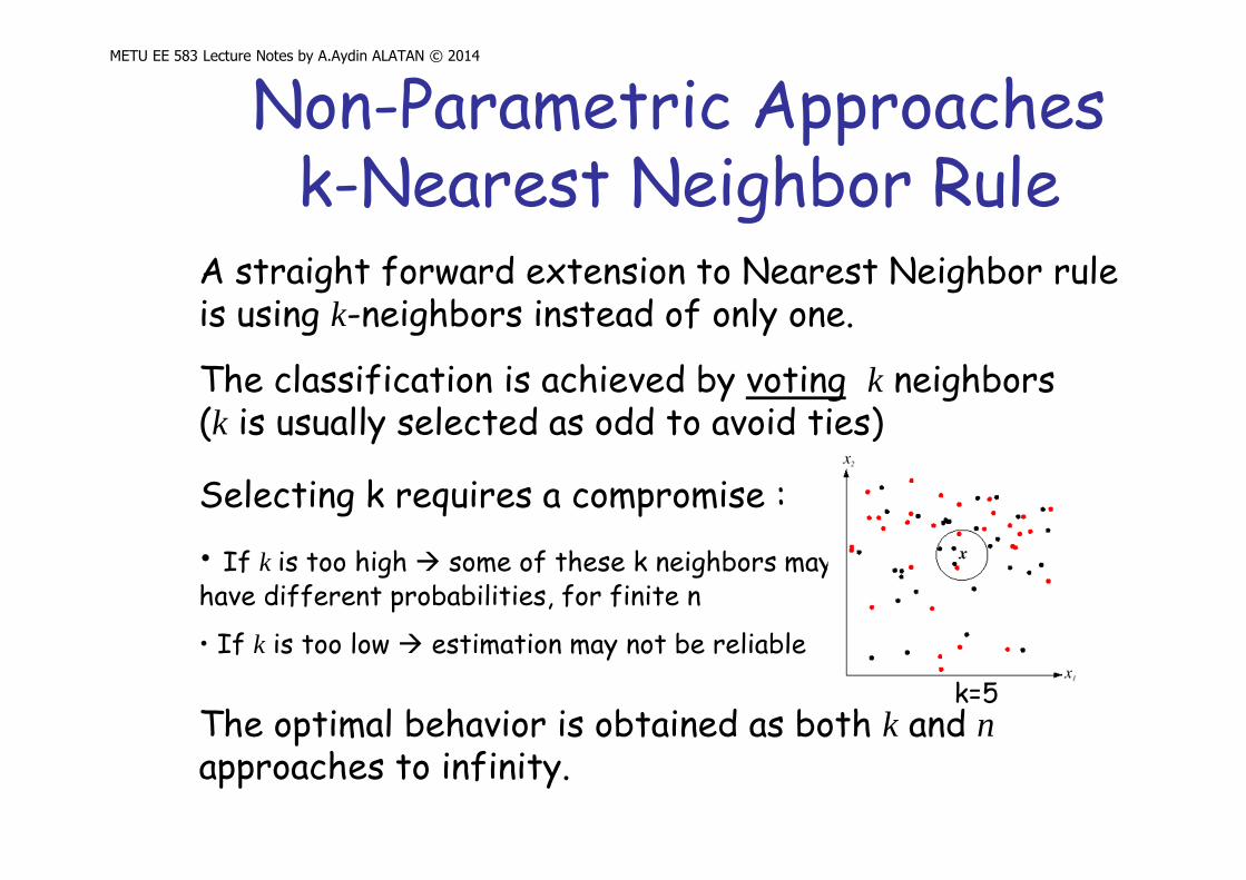
Non-Parametric Approachesk-Nearest Neighbor Rule
A straight forward extension to Nearest Neighbor rule is using k-neighbors instead of only one.
The classification is achieved by voting k neighbors (k is usually selected as odd to avoid ties)
Selecting k requires a compromise :
• If k is too high � some of these k neighbors may have different probabilities, for finite n
• If k is too low � estimation may not be reliable
The optimal behavior is obtained as both k and napproaches to infinity.
k=5
METU EE 583 Lecture Notes by A.Aydin ALATAN © 2014
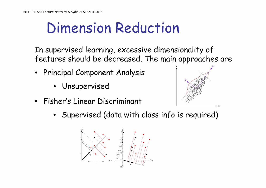
Dimension Reduction
In supervised learning, excessive dimensionality of features should be decreased. The main approaches are
• Principal Component Analysis
• Unsupervised
• Fisher’s Linear Discriminant
• Supervised (data with class info is required)
METU EE 583 Lecture Notes by A.Aydin ALATAN © 2014
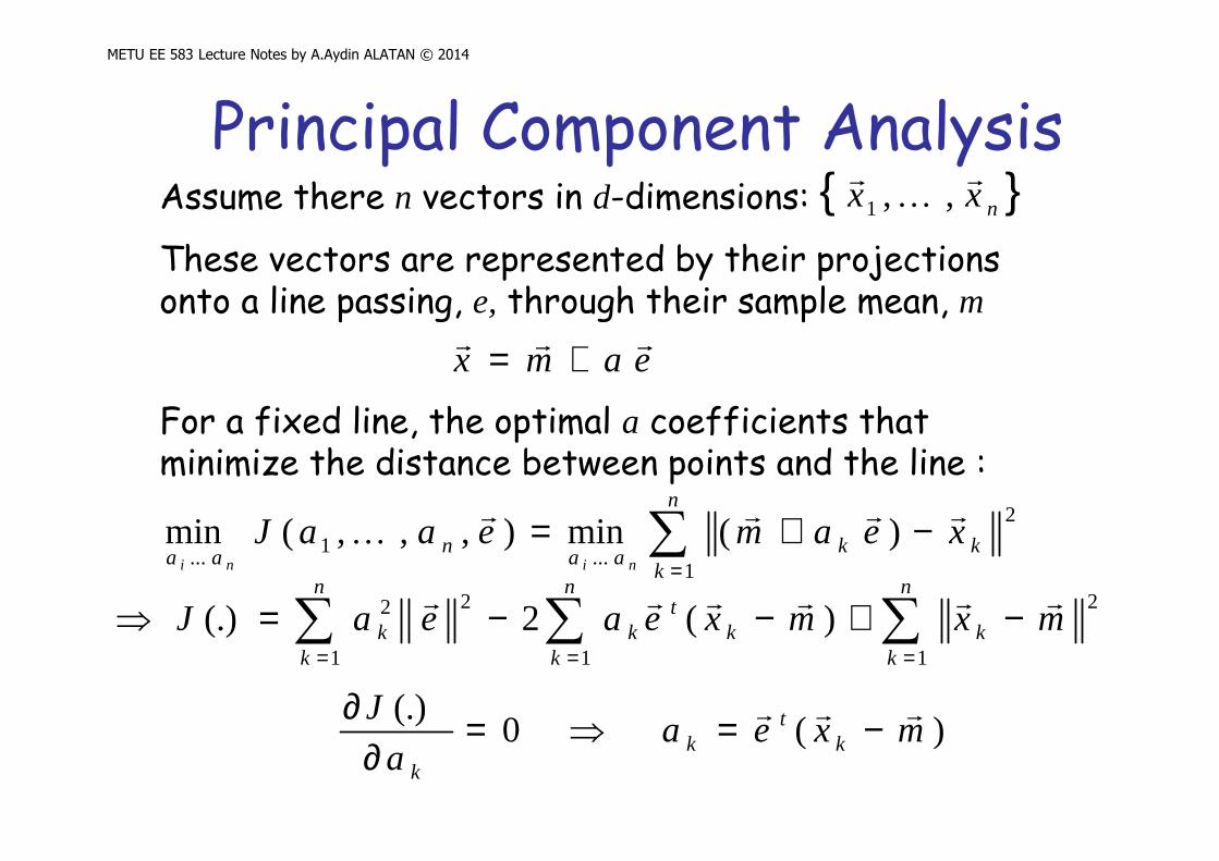
Principal Component Analysis
eamxrrr +=
Assume there n vectors in d-dimensions:
These vectors are represented by their projections onto a line passing, e, through their sample mean, m
{ }nxxr
K
r
,,1
For a fixed line, the optimal a coefficients that minimize the distance between points and the line :
∑=
−+=n
kkk
aan
aaxeameaaJ
nini 1
2
...1
...)(min),,,(min
rrrr
K
∑∑ ∑== =
−+−−=⇒n
kk
n
k
n
kk
tkk mxmxeaeaJ
1
2
1 1
22 )(2(.)rrrrrr
)(0(.)
mxeaa
Jk
tk
k
rrr −=⇒=∂
∂
METU EE 583 Lecture Notes by A.Aydin ALATAN © 2014
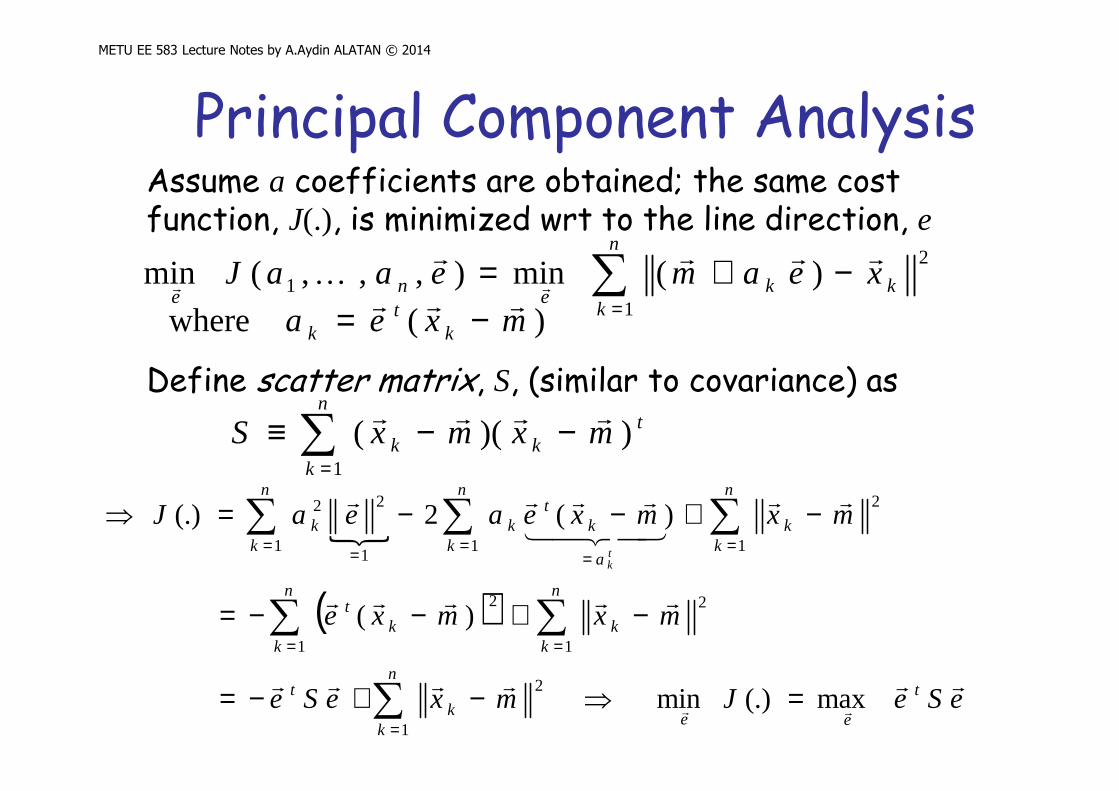
Principal Component Analysis
∑=
−−≡n
k
tkk mxmxS
1
))((rrrr
Assume a coefficients are obtained; the same cost function, J(.), is minimized wrt to the line direction, e
Define scatter matrix, S, (similar to covariance) as
∑=
−+=n
kkk
en
exeameaaJ
1
2
1 )(min),,,(minrrrr
Krr
{
( )
eSeJmxeSe
mxmxe
mxmxeaeaJ
t
ee
n
kk
t
n
kk
n
kk
t
n
kk
n
k
n
ka
kt
kk
tk
rrrrrr
rrrrr
rr
43421
rrrr
rr
max(.)min
)(
)(2(.)
1
2
1
2
1
2
1
2
1 11
22
=⇒−+−=
−+−−=
−+−−=⇒
∑
∑∑
∑∑ ∑
=
==
== ===
)(where mxea kt
k
rrr −=

METU EE 583 Lecture Notes by A.Aydin ALATAN © 2014
Principal Component Analysis
Maximum of etSemust be obtained by the constraint |e|=1
Solution is equal to e which is the eigenvector of S, corresponding its largest eigenvalue
eSeJ t
ee
rr
rr
max(.)min =
0220)1( :mul. Lagrange =−⇒=∂∂
⇒−+≡ eeSe
ueeeSeu tt rrrrrr λλ
Result can be generalized to d’-dimensional projection by minimizing the following relation
∑ ∑=
′
=′ −
+=n
kk
d
iikid xeamJ
1
2
1
rr
i
d
ii eamxrrr
∑′
=
+=1
where , such that ei’s are eigenvectors

METU EE 583 Lecture Notes by A.Aydin ALATAN © 2014
Principal Component Analysis
fXfXXXffXX tX
trrrr
λλ =⇒=left from by multiply
� instead of solving Se=λe or XXte=λe, try solving
Remember n vectors in d-dimensions:
Note difficulty during calculation of S, if d>>n (Sis dxd)
[ ]nxxXr
K
r
,,1=
tn
k
tkk XXmxmxS =−−≡ ∑
=1
))((rrrr
Note that XXt is dxd, whereas XtX is nxn
efX
eeXXfXfXXX tt
r
r
rr
rr
=⇒
=⇔= λλ )()(

METU EE 583 Lecture Notes by A.Aydin ALATAN © 2014
Fisher’s Linear Discriminant (1/8)� The Fisher’s approach aims to project d-dimensional
data onto a line (1-D), which is defined by w
� The projected data is expected to be well separated between two classes after such a dimension reduction

METU EE 583 Lecture Notes by A.Aydin ALATAN © 2014
� Feature vector projections : nixwy it
i ,,1Krr ==
� Measures for separation based on w : � Difference between projection means
� Variance of within-class projection data
� Choose projection (w) in order to maximize J
( ) scatter :
classfor means projection : where
)()(
22
22
21
221
∑∈
−=
+−=•
iYyii
i
mys
im
ss
mmJ
Fisher’s Linear Discriminant (2/8)

METU EE 583 Lecture Notes by A.Aydin ALATAN © 2014
� Relation between sample & projection means :
� Define scatter matrices Si
it
x
t
iYyii
xii mwxw
ny
nmx
nm
iii
rrrrrr
∑∑∑ℵ∈∈ℵ∈
===⇒= 111
� Note that si and Si are related as
( )( ) 21 SSSandmxmxS Wx
Tiii
i
+=−−= ∑ℵ∈
rrrr
Fisher’s Linear Discriminant (3/8)
( ) ( )
( )( ) wSwwmxmxw
mwxwmys
i
ii
xi
TTii
T
xi
TT
Yyii
rrrrrrrr
rrrr
∑
∑∑
ℵ∈
ℵ∈∈
=−−=
−=−= 222

METU EE 583 Lecture Notes by A.Aydin ALATAN © 2014
� This function can be written as
� Similarly, the relation between m1 and m2 becomes
Fisher’s Linear Discriminant (4/8)
22
21
221 )(
)(ss
mmJ
+−=•
wSw
wmmmmwmwmwmm
BT
TTTT
rr
rrrrrrrrrr
=
−−=−=− ))(()()( 21212
212
21
� The initial criterion function :
wSw
wSwwJ
WT
BT
rr
rr
r =)(
� w vector maximizes J must satisfy wSwS WB
rr λ=
� If SW is non-singular, then
{
)( 2111
21
mmSwwwSS W
mmdirection
BW
rrrrr
rr
−=⇒= −
−
− λ
(see distributed notes for its proof)
(Note that SB has rank 1)

METU EE 583 Lecture Notes by A.Aydin ALATAN © 2014
� For a 2-class problem, d-dimensional data is projected on a line
� As an extension to c-class problem, it is possible to project data onto (c-1)-dimensions, instead of a line.
� For (c-1)-dimensions :
� Define new scatter matrices in d-dimensional space
xWycixwy TTii
rr
K
rr =⇒−== 1,1,
( )( )
( )( )
( )( )∑
∑∑
∑∑
=
= ∈
=∈
−−=+=
−+−−+−=
=−−=
c
i
TiiiBBW
c
i Dx
Tiiii
c
iiW
Wholex
TT
mmmmnSSS
mmmxmmmx
SSmxmxS
i
1
1
1
where
,
rrrr
rrrrrrrr
rrrr
r
r
Fisher’s Linear Discriminant (5/8)
(Note that SB has rank c-1)
METU EE 583 Lecture Notes by A.Aydin ALATAN © 2014
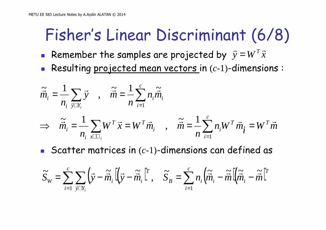
� Remember the samples are projected by
� Resulting projected mean vectors in (c-1)-dimensions :
xWy T rr =
Fisher’s Linear Discriminant (6/8)
mWimWnn
mmWxWn
m
mnn
myn
m
TTc
iii
T
x
T
ii
i
c
ii
Yyii
i
i
rrrrrr
rrrr
r
====⇒
==
∑∑
∑∑
=ℵ∈
=∈
1
1
1~,
1~
~1~,
1~
� Scatter matrices in (c-1)-dimensions can defined as
( )( ) ( )( )∑∑∑== ∈
−−=−−=c
i
T
iiiB
c
i Yy
T
iiW mmmmnSmymySi 11
~~~~~,
~~~ rrrrrrrr
r
METU EE 583 Lecture Notes by A.Aydin ALATAN © 2014
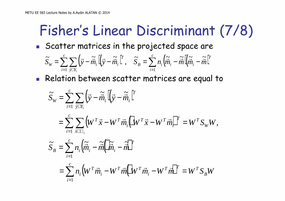
� Scatter matrices in the projected space are
Fisher’s Linear Discriminant (7/8)
� Relation between scatter matrices are equal to
( )( ) ( )( )∑∑∑== ∈
−−=−−=c
i
T
iiiB
c
i Yy
T
iiW mmmmnSmymySi 11
~~~~~,
~~~ rrrrrrrr
r
( )( )
( )( )
( )( )( )( ) WSWmWmWmWmWn
mmmmnS
WSWmWxWmWxW
mymyS
BT
c
i
TTi
TTi
Ti
c
i
T
iiiB
c
i xW
TT
iTT
iTT
c
i Yy
T
iiW
i
i
=−−=
−−=
=−−=
−−=
∑
∑
∑∑
∑∑
=
=
= ℵ∈
= ∈
1
1
1
1
~~~~~
,
~~~
rrrr
rrrr
rrrr
rrrr
r
r

METU EE 583 Lecture Notes by A.Aydin ALATAN © 2014
Fisher’s Linear Discriminant (8/8)� Relation between scatter matrices are obtained as
||
||)(
|~
|
|~
|)(
tdeterminan:. |~
|max&|~
|min
WSW
WSWWJ
S
SJ
SS
WT
BT
W
B
BW
=⇒=•⇒
Note that determinant is product of scatter along principal directions
iWiiB wSwSrr λ=
WSWSWSWS BT
BWT
W == ~,
~
� For better discrimination in the projected space:
� Solution for J(W) : Columns of the optimal W are generalized (c-1) eigenvectors that correspond to the largest eigenvalues of