
EE 380 Linear Control Systems Lecture...
30
EE 380 Fall 2014 Lecture 12. EE 380 Linear Control Systems Lecture 12 Professor Jeffrey Schiano Department of Electrical Engineering 1
Transcript of EE 380 Linear Control Systems Lecture...

EE 380 Fall 2014Lecture 12.
EE 380
Linear Control Systems
Lecture 12
Professor Jeffrey SchianoDepartment of Electrical Engineering
1

EE 380 Fall 2014Lecture 12.
Lecture 12 Topics
• Nonlinear System Analysis– Small-signal Analysis– Chapter 9, Sections 9.1 and 9.2
2

EE 380 Fall 2014Lecture 12.
Fundamental Definitions• A system is said to be linear if the following are true
1. The response can be represented as the sum a zero-input and zero-state response
2. The zero-input response obeys the principle of superposition with respect to the initial state
3. The zero-state response obeys the principle of superposition with respect to the input
• If a system does not satisfy all three properties, then it is nonlinear
3

EE 380 Fall 2014Lecture 12.
Example 1
• Determine if the following systems are zero-state linear
4
2
2
2
2
1
1
(1)
(2) sin(
(
)
)
( )
o
o
d y dya dtdtd y dya ydtd
u
a tt
a y t
u

EE 380 Fall 2014Lecture 12.
Example 1 Solution
5

EE 380 Fall 2014Lecture 12.
Control Design for Nonlinear Plants• Most physical systems are inherently nonlinear
• Control design techniques that account for nonlinear plant behavior are beyond the scope of EE 380
• In many applications it is possible to develop a linear model that approximates the behavior of the nonlinear system for small variations about an operating point
• Given a linear small signal-plant model, one can design a linear feedback system using methods from EE 380
6

EE 380 Fall 2014Lecture 12.
Nonlinear Plant Representation• From Lecture 4, an arbitrary time-invariant nonlinear
system can be represented by the state space model
7
,
,
x f x u
y g x u
1 1 1 1 ,, , , ( , )
,n n m n
x x u f x ux x u f x u
x x u f x u
1 1 ,, ( , )
,r r
y g x uy g x u
y g x u

EE 380 Fall 2014Lecture 12.
Example 2
• Determine a state-space representation for a pendulum with damping at the pivot point. Is the system linear?
8
M
B

EE 380 Fall 2014Lecture 12.
Example 2 Solution
9

EE 380 Fall 2014Lecture 12.
Static Equilibrium States• Consider the time-invariant nonlinear system
• Drive the system with a constant input
• The constant state vector(s) xe satisfying
are called static equilibrium states
• In many cases, the constant input uo and equilibrium state xe represent a desired operating point
10
( ) ou t u
,x f x u
10 ,n e of x u

EE 380 Fall 2014Lecture 12.
Example 3
• Determine the static equilibrium state(s) of the pendulum system considered in example 2
11
M
B

EE 380 Fall 2014Lecture 12.
Example 3 Solution
12

EE 380 Fall 2014Lecture 12.
Stability of Static Equilibrium States
13
• Once in a static equilibrium state, if left unperturbed, the system remains in that state because dx/dt = 0
• The equilibrium state xe is said to be stable if for small perturbations from xe, the system returns to the equilibrium state
• The equilibrium state xe is said to be unstable if for small perturbations from xe, the system diverges from xe

EE 380 Fall 2014Lecture 12.
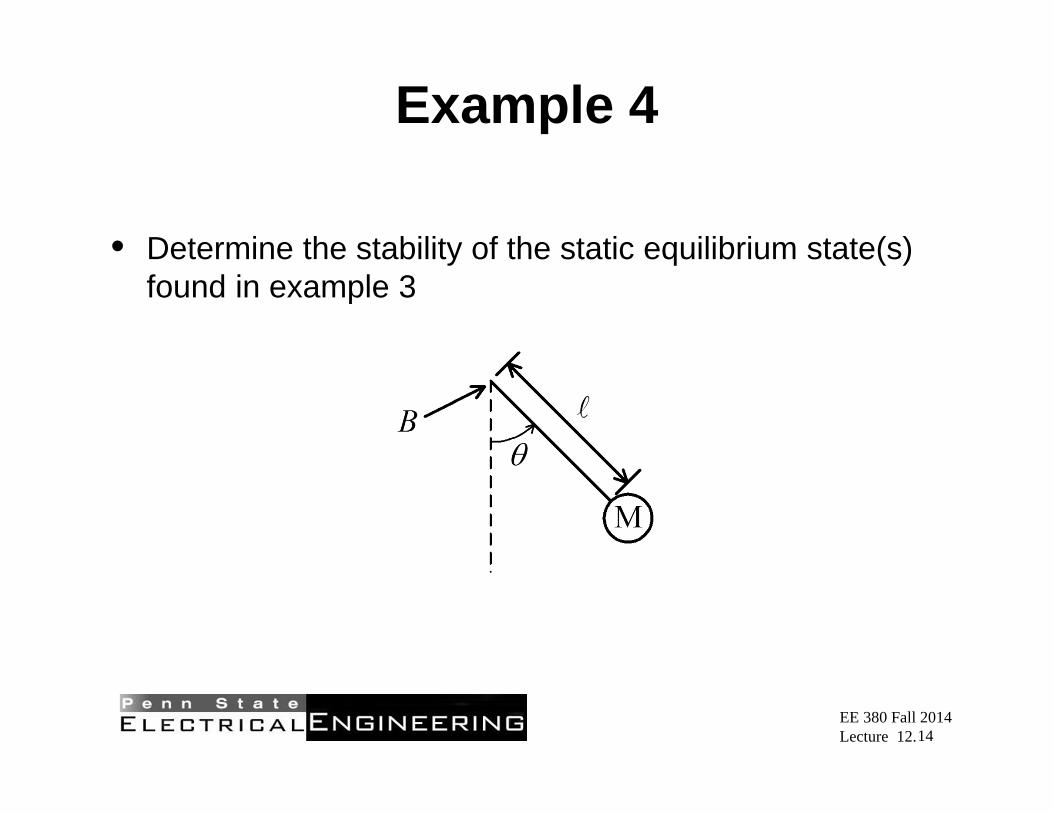
Example 4
• Determine the stability of the static equilibrium state(s) found in example 3
14
M
B

EE 380 Fall 2014Lecture 12.
Example 4 Solution
15

EE 380 Fall 2014Lecture 12.
EE 380
Linear Control Systems
Lecture 12
Professor Jeffrey SchianoDepartment of Electrical Engineering
1

EE 380 Fall 2014Lecture 12.
Lecture 12 Topics
• Nonlinear System Analysis– Small-signal Analysis– Chapter 9, Sections 9.1 and 9.2
2

EE 380 Fall 2014Lecture 12.
Fundamental Definitions• A system is said to be linear if the following are true
1. The response can be represented as the sum a zero-input and zero-state response
2. The zero-input response obeys the principle of superposition with respect to the initial state
3. The zero-state response obeys the principle of superposition with respect to the input
• If a system does not satisfy all three properties, then it is nonlinear
3

EE 380 Fall 2014Lecture 12.
Example 1
• Determine if the following systems are zero-state linear
4

EE 380 Fall 2014Lecture 12.
Example 1 Solution
5

EE 380 Fall 2014Lecture 12.
Control Design for Nonlinear Plants• Most physical systems are inherently nonlinear
• Control design techniques that account for nonlinear plant behavior are beyond the scope of EE 380
• In many applications it is possible to develop a linear model that approximates the behavior of the nonlinear system for small variations about an operating point
• Given a linear small signal-plant model, one can design a linear feedback system using methods from EE 380
6

EE 380 Fall 2014Lecture 12.
Nonlinear Plant Representation• From Lecture 4, an arbitrary time-invariant nonlinear
system can be represented by the state space model
7

EE 380 Fall 2014Lecture 12.
Example 2
• Determine a state-space representation for a pendulum with damping at the pivot point. Is the system linear?
8

EE 380 Fall 2014Lecture 12.
Example 2 Solution
9

EE 380 Fall 2014Lecture 12.
Static Equilibrium States• Consider the time-invariant nonlinear system
• Drive the system with a constant input
• The constant state vector(s) xe satisfying
are called static equilibrium states
• In many cases, the constant input uo and equilibrium state xe represent a desired operating point
10

EE 380 Fall 2014Lecture 12.
Example 3
• Determine the static equilibrium state(s) of the pendulum system considered in example 2
11

EE 380 Fall 2014Lecture 12.
Example 3 Solution
12

EE 380 Fall 2014Lecture 12.
Stability of Static Equilibrium States
13
• Once in a static equilibrium state, if left unperturbed, the system remains in that state because dx/dt = 0
• The equilibrium state xe is said to be stable if for small perturbations from xe, the system returns to the equilibrium state
• The equilibrium state xe is said to be unstable if for small perturbations from xe, the system diverges from xe
EE 380 Fall 2014Lecture 12.
Example 4
• Determine the stability of the static equilibrium state(s) found in example 3
14

EE 380 Fall 2014Lecture 12.
Example 4 Solution
15


